Quantum Gravity with Matter
via Group Field Theory

Abstract.

A generalization of the matrix model idea to quantum gravity in three and higher dimensions is known as group field theory (GFT). In this paper we study generalized GFT models that can be used to describe 3D quantum gravity coupled to point particles. The generalization considered is that of replacing the group leading to pure quantum gravity by the twisted product of the group with its dual –the so-called Drinfeld double of the group. The Drinfeld double is a quantum group in that it is an algebra that is both non-commutative and non-cocommutative, and special care is needed to define group field theory for it. We show how this is done, and study the resulting GFT models. Of special interest is a new topological model that is the “Ponzano-Regge” model for the Drinfeld double. However, as we show, this model does not describe point particles. Motivated by the GFT considerations, we consider a more general class of models that are defined using not GFT, but the so-called chain mail techniques. A general model of this class does not produce 3-manifold invariants, but has an interpretation in terms of point particle Feynman diagrams.

1. Introduction

Recently a question of coupling of quantum gravity to matter has been revisited in works [1, 2]. Both papers deal with quantum gravity in 2+1 dimensions, and analyze how matter Feynman diagrams are modified when the quantum gravity effects are taken into account. Both work contain results that are intriguing. However, certain conceptual issues were left unclear. Thus, work [1] has suggested that the effect of quantum gravity is in modifying the measure of integration $\prod_{v}dx_{v}$ in a Feynman amplitude given by:

$${\mathcal{Z}}=\int\prod_{v}dx_{v}\prod_{\langle vv^{\prime}\rangle}G(x_{v}-x_{v^{\prime}}).$$ (1.1)

Here one integrates over the positions of vertices $x_{v}$ of a Feynman graph, $G(x-y)$ is the particle propagator in coordinate representation, and $\langle vv^{\prime}\rangle$ denotes edges of the Feynman diagram. In this scheme quantum gravity is only responsible for a modification of the $\prod_{v}dx_{v}$ measure, and the particle content as well as the Lagrangian must be specified independently. In particular, one is not forced to using any particular propagator. Thus, this proposal is that of “quantum gravity + matter”. Work [2], on the other hand, showed that particular quantum gravity amplitudes can be interpreted as particle Feynman diagrams, provided one makes a special choice of the particle propagator. Thus, in this interpretation “quantum gravity = matter”. These two interpretations seem to be in conflict. This paper is devoted to an analysis of these and related issues. We will argue that both interpretations are correct.

The basic philosophy that is to be pursued in the present paper is as follows. Consider the momentum representation Feynman amplitude of some theory. The precise definition of the theory is unimportant for us at this stage. We shall restrict our attention to general aspects common to Feynman amplitudes of all theories. Thus, the amplitude is given by:

$${\mathcal{Z}}=\int\prod_{\langle vv^{\prime}\rangle}dp_{\langle vv^{\prime}\rangle}G(p_{\langle vv^{\prime}\rangle})\prod_{v}\delta(\sum_{v^{\prime}}p_{\langle vv^{\prime}\rangle}).$$ (1.2)

Here the integrals are taken over the momenta $p_{\langle vv^{\prime}\rangle}$ on each edge of the digram; in addition, one has a momentum conservation law for each vertex. We have to modify the Feynman amplitude (1.2) so that it describes point particles. Point particles in 2+1 dimensions are conical singularities in the metric. As we shall see, this has the effect that particle’s momentum is group-valued. For point particles in Euclidean 3-dimensional space, which is what we consider in this work, the relevant group is $\operatorname{SU}(2)$. The proposal to be developed in this paper is that point particles and processes involving them can still be described by Feynman diagrams (1.2), but the momentum $p$ on each edge of the diagram should be taken group-valued. The rest of the paper is devoted to various tests of this proposal.

Some point particle theories we consider are topological; we refer the reader to the main body of the paper for the precise definition of what this means. As we shall see, these topological particle theories will be produced by the GFT. Other theories we consider are non-topological; GFT is of no direct relevance here. However, the techniques developed in the GFT context (such as the chain mail, see below) will prove extremely useful for these theories as well. This is how the GFT is omnipresent throughout the paper.

We start by reminding the reader how point particles in 3D are described. For simplicity, this paper deals only with the case of $3+0$-dimensional spacetime, that is, with 3D metrics of Euclidean signature, and the cosmological constant is set to zero.

1.1. Point particles

In 3 spacetime dimensions presence of matter has much more drastic consequences than in 4D: the asymptotic structure of spacetime gets modified. This has to do with the fact that the vacuum Einstein equations are much stronger in 3D: they require that the curvature is constant (zero) everywhere. Then an asymptotically flat spacetime is flat everywhere. When matter is placed inside it introduces a conical defect that can be felt at infinity. The modification due to matter is in the leading order, not in the next to leading as in higher dimensions. This has the consequence that the total mass in spacetime is proportional to the deficit angle created at infinity. Because the angle deficit cannot increase $2\pi$, the mass is bounded from above. All this is very unlike the case of higher dimensions, and makes the theory of matter look rather strange and unfamiliar. But such strange features are at the end of the day responsible for a complete solubility of the theory.

Point particles give the simplest and most natural form of matter to consider in 3D. A point particle creates a conical singularity at the point where it is placed. The angle deficit $2\theta$ at the tip of the cone is related to particle’s mass as $4\pi MG=\theta$. Point particles move along geodesics. Their worldliness are lines of conical singularities.

To make this description more explicit, let us consider how a space containing a line of conical singularity can be obtained. This is achieved by performing a rotation of space, and identifying points related by this rotation. A rotation is described by an element $g(2\theta)\in\operatorname{SU}(2)$, which we choose to parameterize as follows:

$$g(\theta)=e^{i\theta\vec{n}\cdot\vec{\sigma}}=\cos{\theta}+i\vec{n}\cdot\vec{\sigma}\sin{\theta}.$$ (1.3)

Here $\vec{n}:\vec{n}\cdot\vec{n}=1$ is a unit vector. It describes the direction of the axis of rotation, and thus the direction of particle’s motion. The angle $2\theta$ specifies the amount of rotation, and thus gives the mass of the particle. The reason for choosing $\theta$ and not $2\theta$ for parameterizing the particle’s mass will become clear below. An equivalent description in more mathematical terms is to say that a particle of a given mass $\theta$ is described by a group element $g\in C_{\theta}$, where $C_{\theta}$ is a conjugacy class in $\operatorname{SU}(2)$. Non-trivial conjugacy classes $C_{\theta},\theta\not=0$ in $\operatorname{SU}(2)$ are spheres $S^{2}$ and a point in $C_{\theta}$ describes the direction of motion. Thus, the information about both the mass and the direction of motion is encoded in $g$. This is why this quantity plays the role of momentum of a point particle. Note that the group-valued nature of particle’s momentum automatically incorporates the bound on its mass. Note also that not only the upper, but the lower bound is naturally imposed as well – the $\operatorname{SU}(2)$ valued momenta are those of non-negative mass particles.

Once points of $\mathbb{R}^{3}$ related by a rotation $g$ are identified, we obtain a space with a line of conical singularity in the direction $\vec{n}$. The angle deficit is $2\theta$. The space has zero curvature everywhere except along particle’s worldline. One can compute the holonomy of the spin connection around the worldline and verify that it is equal to $g(\theta)$. It is for this reason that the quantity $\theta$ equal to half the angle deficit gives a more convenient measure parameterization of the mass. Let us now consider two point particles, with group elements $g_{1},g_{2}$ describing them. The holonomy around the pair is the product of holonomies, and the mass parameter $\theta$ of the pair is given by:

$$\cos{\theta}=\frac{1}{2}\operatorname{Tr}(g_{1}g_{2})=\cos{\theta_{1}}\cos{\theta_{2}}-\vec{n_{1}}\cdot\vec{n_{2}}\sin{\theta_{1}}\sin{\theta_{2}}.$$ (1.4)

Note that it does matter now in which order the product of holonomies is taken, for $g_{1}g_{2}\not=g_{2}g_{1}$ as we are dealing with elements of the group. But in determining the mass of the combined system this ambiguity is irrelevant, for the trace is taken. Let us look at (1.4) in more detail. In case $\vec{n_{1}}$ is parallel to $\vec{n_{2}}$, this formula reduces to: $\theta=\theta_{1}+\theta_{2}$. When particles move in opposite directions we have: $\theta=|\theta_{1}-\theta_{2}|$. Thus, the angle $\theta$ is more properly interpreted as the magnitude of particle’s momentum, not as its kinetic energy.

It is instructive to compare (1.4) to the usual law of addition of vectors in $\mathbb{R}^{3}$. Thus, consider two particles with momenta $\vec{p_{1}},\vec{p_{2}}$. Define: $m=|\vec{p}|,\vec{n}=\vec{p}/|\vec{p}|$. Then we have:

$$m^{2}=m_{1}^{2}+m_{2}^{2}+2\vec{n_{1}}\cdot\vec{n_{2}}m_{1}m_{2}.$$ (1.5)

This formula for addition of momenta is to be compared with (1.4). Indeed, as $\theta=4\pi MG$, (1.4) can be expanded in powers of $G$. This gives exactly (1.5), modified by $O(G^{2})$ corrections:

$$M^{2}=M_{1}^{2}+M_{2}^{2}+2\vec{n_{1}}\cdot\vec{n_{2}}M_{1}M_{2}+$$ (1.6)

$$\frac{4\pi^{2}G^{2}}{3}\left(M^{4}-M_{1}^{4}-M_{2}^{4}-3M_{1}^{2}M_{2}^{2}-4\vec{n_{1}}\cdot\vec{n_{2}}M_{1}M_{2}(M_{1}^{2}+M_{2}^{2})\right)+O(G^{4}).$$

Thus, the fact that the law (1.4) of addition of momenta has the correct limit as $G\to 0$ gives additional support to our identification of $g$ with particle’s momentum.

Having understood why particle’s momentum becomes group valued, let us remind the reader some basic facts about the Ponzano-Regge model [3] of 3D quantum gravity, and how point particles can be coupled to it.

1.2. Ponzano-Regge model in presence of conical singularities

In Ponzano-Regge model, one triangulates the 3-manifold in question (“spacetime”), and assigns a certain amplitude to each triangulation. This amplitude turns out to be triangulation independent and gives a topological invariant of the 3-manifold. Let us remind the reader how the Ponzano-Regge amplitude (1.11) can be obtained from the gravity action. When written in the first order formalism, zero cosmological constant 3D gravity becomes the so-called BF theory. The action is given by:

$$S[{\bf e},{\bf a}]=\int_{M}{\rm Tr}({\bf e}\wedge{\bf f}).$$ (1.7)

Here $\bf e$ is a Lie algebra valued one form, and $\bf f$ is the curvature of a $G$-connection $\bf a$ on $M$. The path integral of this simple theory reduces to an integral over flat connections:

$${\mathcal{Z}}[M]=\int{\mathcal{D}}{\bf e}{\mathcal{D}}{\bf a}\,\,e^{iS[{\bf e},{\bf a}]}=\int{\mathcal{D}}{\bf a}\,\,\delta({\bf f}).$$ (1.8)

A discretized version of this last integral can be obtained as follows. Let us triangulate the manifold $M$ in question. Let us associate with every edge of the dual triangulation the holonomy matrix for the connection $\bf a$. This holonomy matrix is an element of the group $G$. The product of these holonomies around the dual face must give the trivial element (because the connection is flat). Thus, one can take the $\delta$-function of a product of group elements around each dual face, multiply these $\delta$-functions and then integrate over the group elements on dual edges. This is the discretized version of (1.8). By decomposing the $\delta$-function on the group $G=\operatorname{SU}(2)$ into characters, it is easy to show that this procedure gives the following amplitude:

$$\sum_{\{j_{e}\}}\prod_{e}{\rm dim}(j_{e})\prod_{t}(6j).$$ (1.9)

It turns out, however, that this amplitude is not yet triangulation independent. In order to make it such one has to introduce a certain formal prefactor. Thus, let us consider the following sum over irreducible representations of $\operatorname{SU}(2)$:

$$\eta^{-2}:=\sum_{j}{\rm dim}_{j}^{2}.$$ (1.10)

Note that this sum diverges and the quantity $\eta$ defined by it is formal. The sum above is equal to the $\delta$-function on the group evaluated at the identity element. To make the amplitude (1.9) triangulation independent one has to consider the following multiple of it:

$$\eta^{2V}\sum_{\{j_{e}\}}\prod_{e}{\rm dim}(j_{e})\prod_{t}(6j),$$ (1.11)

where $V$ is the number of vertices in the triangulation used to obtain (1.9). The amplitude (1.11) is now (formally, because of a prefactor that is actually equal to zero) triangulation independent.

The origin of this formal prefactor is now well-understood, see [4]. It has to do with the fact that the action (1.7) in addition to the usual $\operatorname{SU}(2)$ gauge symmetry has a non-compact gauge-symmetry. Indeed, because of the Bianchi identity $d_{A}F=0$ the action is invariant under the following transformation: $B\to B+d_{A}\phi$. Integration over $B$ in the path integral includes integration over these gauge directions and produces infinities that has to be cancelled by the zero prefactor in (1.11). A more systematic procedure for dealing with these divergences was developed in [4, 6] and requires a certain gauge fixing procedure. We shall not consider such a gauge fixing here and will proceed at a formal level, just keeping track of the (formal) pre-factors $\eta$. All amplitudes can be rendered well-defined by passing to the quantum group context, that is, by considering the quantum group $\operatorname{SU}_{q}(2)$ instead of $\operatorname{SU}(2)$. When $q$ is a root of unity the cut-off on the spin present in the representation theory of $\operatorname{SU}_{q}(2)$ makes the sum that defines $\eta^{-2}$ finite, and all the invariants well-defined. One should always have this passage to $\operatorname{SU}_{q}(2)$ in mind when considering the ill-defined Ponzano-Regge model expressions.

We have explained how the amplitude in (1.11) can be obtained from an integral over flat connections. It is now easy to add a point particle. Consider the case when a point particle is present and (a segment of) its worldline coincides with one of the edges of the triangulation of $M$. It will then create a conical singularity along this edge. The product of holonomies around the face dual to this edge is not trivial anymore. Instead it will lie in a conjugacy class determined by the mass of the particle (by its deficit angle). Thus, for dual edges that encircle particles’ worldline one should put a $\delta$-function concentrated on the conjugacy class determined by the particle. This gives a modified amplitude, with presence of the point particle taken into account. Let us introduce a $\delta$-function that is picked on a particular conjugacy class $\theta$:

$$\delta_{\theta}(x):=\int dg\delta_{e}(gh_{\theta}g^{-1}x)=\sum_{j}\chi_{j}(h_{\theta})\chi_{j}(x).$$ (1.12)

Here $\delta_{e}(x)$ is the usual $\delta$-function on the group picked at the identity element. The sum in the second formula is taken over all irreducible representations of the group $\operatorname{SU}(2)$, and $\chi_{j}(g)$ are the characters. The special group element $h_{\theta}$ is a representative of the conjugacy class $\theta:h_{\theta}={\rm diag}(\exp{i\theta},\exp{-i\theta})$. Note that when $\theta=0$, the above $\delta$-function reduces to the usual $\delta$-function picked at the identity. Let us now assume that a point particle is present along all the edges of the triangulation, and denote the angle deficit on the edge $e$ by $\theta_{e}$. The modified quantum gravity amplitude in the presence of particles is given by:

$$\sum_{\{j_{e}\}}\prod_{e}\chi_{j_{e}}(h_{\theta_{e}})\prod_{t}(6j).$$ (1.13)

If particles are present along all the edges, there is no need to introduce a formal $\eta$ prefactor as the amplitude is not required to be triangulation independent. If the particle is only present along some of the edges, one gets what can be called an observable of Ponzano-Regge model, see [7]. In this case pre-factors of $\eta$ for vertices away from the particle edges are necessary to ensure a partial triangulation independence, see [7] for more details.

As it was explained in [1] and [2], the amplitude (1.13) is the response of the quantized gravitational field to particle’s presence. In the setting described the particle is present as en external source in the gravitational path integral. The natural question is if one can integrate over the particle degrees of freedom and thus have a quantum theory of particles coupled to quantum gravity. In other words, the question is how to “second quantize” the particle degrees of freedom. Some sketches on how this can be done were presented in both [1] and [2]. What is missing in these papers is a principle that would generate Feynman diagrams for both gravity and particle degrees of freedom. This paper is aimed at filling this gap. As we shall see, the Feynman amplitudes for some of the theories (namely the topological ones) can be generated by GFT. To understand how this is possible, let us remind the reader some basic facts about the usual field theory Feynman diagrams, and, in particular, about a certain duality transformation that can be performed on a diagram. Let us remark that for the most part this paper deals with vacuum (closed) Feynman diagrams only. A generalization to open diagrams that are essential for doing the scattering theory will be left for future work.

1.3. Momentum representation and duality

In addition to the coordinate (1.1) and momentum (1.2) representations of Feynman diagrams there is another, the so-called dual representation. Let us remind the reader how the dual representation is obtained in the case of two spacetime dimensions. To get the dual formulation we need to endow Feynman graphs with an additional “fat” structure. Namely, each edge of the digram must be replaced by two lines. The fat structure is equivalent to an ordering of edges at each vertex. The lines of the fat graph are then connected at vertices as specified by ordering. This structure is also equivalent to specifying a set of 2-cells, or faces of the diagram. Once this additional structure is introduced, one can define the genus $G$ of the diagram to be given by the Euler formula: $2-2G=V-E+F$, where $V,E,F$ are the numbers of vertices, edges and faces of the diagram correspondingly. Note that the same Feynman diagram can be given different fat structures and thus have different genus. For example, the diagram with 2 tri-valent vertices and 3 edges (the $\theta$-graph) can correspond to both genus zero and genus one after the fat structure is specified.

Having introduced the fat structure, we can solve all the momentum conservation constraints. It is simplest to do it in the case of $G=0$, so let us specialize to this situation. Let us introduce the new momentum variables, one for every face of the diagram. Let us denote these by $p_{f}$. Given a pair $\langle ff^{\prime}\rangle$ of adjacent faces, there is a unique edge $\langle vv^{\prime}\rangle$ that is a part of the boundary of both of them. A relation between the original momentum variables $p_{\langle vv^{\prime}\rangle}$ and the new variables $p_{f}$ is then given by:

$$p_{\langle vv^{\prime}\rangle}=p_{f}-p_{f^{\prime}}.$$ (1.14)

Let us check that the number of new variables is the number of old variables minus the number of constrains. The number of new variable is equal to $F-1$: the number of faces minus one. We have to subtract one because everything depends on the differences only and does not change if we shift all the variables by the same amount. We have $F-1=E-(V-1)-2G=E-(V-1)$, where we have used our assumption that $G=0$. Thus, the number of new variables equals to the number of the original variables, minus the number of $\delta$-functions, equal to $V-1$ because one $\delta$-function is always redundant. In case $G\not=0$ one has to introduce an extra variable for each independent non-contractible loop on the surface, whose number is $2G$. Thus, having expressed the momentum variables via $p_{f}$ using (1.14), we have automatically solved all the conservation constraints. The Feynman amplitude becomes:

$$\int\prod_{f}dp_{f}\prod_{\langle ff^{\prime}\rangle}G(p_{f}-p_{f^{\prime}}).$$ (1.15)

We shall refer to (1.15) as the dual representation of a 2D Feynman diagram. One can perform a similar duality transformation in higher dimensions. The case relevant for us here is that of 3D, so let us briefly analyze what happens. Let us consider a vacuum (closed) Feynman diagram and introduce an additional structure that specifies faces, as well as an ordering of these faces around edges. For example, let us consider Feynman graphs whose edges and vertices are those of a triangulation of spacetime. As we shall soon see, such Feynman diagrams are natural if one wants to interpret the state sum models of 3D quantum gravity in particle terms. The faces of such “triangulation” diagrams are then the usual triangles. As in 2D, let us assign a variable $p_{f}$ to each face. The original edge momentum variable is then expressed as an appropriate sum of the face variables, for all the faces that share the given edge:

$$p_{e}=\sum_{f:e\in f}p_{f}\epsilon_{f}.$$ (1.16)

One sums the face variables $p_{f}$ weighted with sign $\epsilon_{f}$; a precise convention is unimportant for us at the moment. The number of the original variables is $E-(V-1)$, and due to the fact that the Euler characteristic of any 3-manifold is equal to zero, we get: $E-(V-1)=F-(T-1)$, which means that one in addition has to impose $T-1$ constraints for the new variables. Thus, in the original momentum representation we had $E$ edge variables together with the momentum conservation constraints for each vertex. In the dual formulation one has a momentum variable for each dual edge, and one conservation constraint for each dual vertex. We had to switch to the dual lattice in order to solve the $\delta$-function constraints.

1.4. Point particle Feynman diagrams

Here we further develop our proposal of modifying Feynman diagrams by making the momentum group valued. Thus, let us consider some theory of point particles in 3D that generates Feynman diagrams. A form of the action is unimportant for us. Our starting point will be diagrams in the momentum representation. As we have already described, the most unusual feature of point particles in 3D is that their momentum is group-valued and thus non-commutative. Thus, point particles in 3D behave unlike the standard relativistic fields in Minkowski spacetime. In spite of this, one can still consider Feynman diagrams. Indeed, in the momentum formulation (1.2) one only needs to specify what the propagator is, what the integration measure $dp$ is, and what replaces the momentum conservation $\delta$-functions. All this objects exist naturally for the 3D point particles. The propagator $G(p)$ is some function on the group $\operatorname{SU}(2)$, which we shall leave unspecified for now. The integration measure is the Haar measure on the group. The momentum conservation is more subtle. The conservation constraint becomes the condition that the product of the group elements $g_{\langle vv^{\prime}\rangle}$ for all $v^{\prime}$ is equal to the identity group element. However, it now does matter in which order the group elements are multiplied. Thus, some additional structure is necessary to define the momentum conservation constraints and Feynman amplitude as a whole. We shall specify this additional structure below. Ignoring this issue for the moment we get:

$${\mathcal{Z}}=\int\prod_{\langle vv^{\prime}\rangle}dg_{\langle vv^{\prime}\rangle}G(g_{\langle vv^{\prime}\rangle})\prod_{v}\delta\left(\prod_{v^{\prime}}g_{\langle vv^{\prime}\rangle}\right).$$ (1.17)

Here $g_{e}=g_{\langle vv^{\prime}\rangle}\in\operatorname{SU}(2)$ is the group element that describes particle’s momentum on edge $e$, $G(g)$ is a propagator which is a function on the group $\operatorname{SU}(2)$, and $\delta(g)$ is the usual $\delta$-function on the group picked at the identity element.

Let us now deal with the issue of defining the momentum conservation constraints. It is clear that some additional structure is necessary. We have already seen an extra structure being added to a Feynman diagram when we considered the dual formulation. In that case an extra structure was introduced to solve the momentum constraints. It is clear that exactly the same structure can be used to define these constraints in the case of group-valued momenta. Thus, let us introduce an extra structure of faces, as well as ordering of faces around each edge. This is equivalent to introducing the structure of a dual complex. For simplicity we shall assume that the Feynman diagram we started from is a triangulation of some manifold. The dual complex is then the dual triangulation. Let us introduce new momentum variables: one for each face of the triangulation. The original edge momentum is expressed as a product of the face variables:

$$g_{e}=\prod_{f:e\in f}g_{f}.$$ (1.18)

The order of the product here is important and is given by the ordering of the faces around the edge: one multiples the holonomies across faces to get the holonomy around the edge. The new face momentum variables $g_{f}$ solve all the vertex momentum conservation constraints. The amplitude (1.17) in the dual formulation becomes:

$${\mathcal{Z}}=\int\prod_{f}dg_{f}\prod_{e}G\left(\prod_{f:e\in f}g_{f}\right)\prod_{t}TC,$$ (1.19)

where $TC$ are the tetrahedral constraints that were shown to be necessary by counting the variables in the previous subsection.

1.5. Tetrahedron constraints

It turns out that the tetrahedron constraints have a simple meaning. The constraints imply that the face variables are not all independent. There is a gauge symmetry that acts at each tetrahedron. At this stage it is convenient to pass to the dual triangulation. Recall that each face is dual to an edge $e$ of the dual triangulation, and each tetrahedron is dual to a vertex $v$. To write down the action of the gauge transformation acting at $v$, let us orient all the edges $e$ incident at this vertex to point away from $v$. Then the action on $g_{e}$ is as follows: $g_{e}\to g_{v}g_{e}$, where $g_{v}$ is the same for all edges $e$ incident at $v$. Fixing this gauge symmetry is the same as imposing the tetrahedron constraints in (1.19). Below we shall see how these constraints can be dealt with.

There is another possible interpretation that can be given to the constraints. Let us consider a geometric tetrahedron in $\mathbb{R}^{3}$. The group valued face variables $g_{f}$ that we have introduced have the meaning of an $\operatorname{SU}(2)$ transformation that has to be carried out when one goes from one tetrahedron of the triangulation to the other. This group element can be represented as a product of two group elements, one for each tet: $g_{f}=(g_{f}^{t})^{-1}g_{f}^{t^{\prime}}$, where $t,t^{\prime}$ are the two tetrahedra that share the face $f$. Consider now: $(g^{t}_{f})^{-1}g^{t}_{f^{\prime}}$. This group element describes the rotation of one face $f$ into another $f^{\prime}$, and thus carries information about the dihedral angle between the two faces. Thus, the group variables $g_{f}$ introduced to solve the momentum constraints carry information about the dihedral angles between the faces of the triangulation. In particular, the total angle $2\pi-\theta_{e}$ on an edge $e$ is just the sum of all the dihedral angles around this edge:

$$2\pi-\theta_{e}=\sum_{\langle ff^{\prime}\rangle}\theta_{ff^{\prime}},$$ (1.20)

where the sum is taken over the pairs $\langle ff^{\prime}\rangle$ of faces that share the edge $e$. This relation should be thought of as contained in the relation (1.18). Having understood the (partial) geometrical meaning of the face variables as encoding the dihedral angles between the faces, we can state the (partial) meaning of the tetrahedron constraints. Recall that 6 dihedral angles of a tetrahedron satisfy one relation. This relation is obtained as follows. Consider the unit normals $\vec{n_{i}},i=1,\ldots,4$ to all 4 faces of the tetrahedron. Let us form a matrix $A_{ij}=\vec{n_{i}}\cdot\vec{n_{j}}$ of products of the normals. It is clear that $\vec{n_{i}}\cdot\vec{n_{j}}=-\cos(\theta_{ij})$, and so the entries of $A_{ij}$ are just the cosines of the dihedral angles. However, as the vectors $\vec{n_{i}}$ are 4 vectors in $\mathbb{R}^{3}$, they must be linearly dependent:

$$\sum_{i}A_{i}\vec{n_{i}}=0.$$ (1.21)

The coefficients $A_{i}$ here are just the areas of the corresponding faces. Because the normals $\vec{n_{i}}$ are linearly dependent the determinant of the matrix $A_{ij}$ is equal to zero, which is the sought constraint among the 6 dihedral angles $\theta_{ij}$. This relation between the dihedral angles should be thought of as contained in the tetrahedron constraints in (1.19).

Let us now consider some example theories to which the above strategy can be applied.

1.6. Pure gravity from point particle Feynman diagrams

One special important case to be considered arises when particle’s propagator is equal to the $\delta$-function of the momentum. Had we been dealing with a usual theory in $\mathbb{R}^{3}$ in which the position and momentum representations are related by the Fourier transform such a choice of the propagator would mean having $G(x-y)=1$ in the position space. Thus, this theory is a trivial one as far as particles are concerned - there are no particles. However, as we shall see in a moment, in the point particle context it leads to a non-trivial and interesting amplitude.

From the perspective of the Feynman amplitude (1.17) it is clear that this case is a bit singular. Indeed, the edge $\delta$-functions guarantee that all the holonomies around edges are trivial. But then the vertex momentum conservation $\delta$-function is redundant, and makes the amplitude divergent. To deal with this divergence, let us consider a modified amplitude with no momentum conservation $\delta$-functions present. An equivalent way of dealing with this problem is to introduce the (formal) quantity $\eta$ given by (1.10). Now we have to divide our amplitude by $\eta^{-2V}$, where $V$ is the number of vertices in the diagram. We can now consider the dual formulation in which all the constraints are solved. Let us keep the factors of $\eta$, for they are going to be an important part of the answer that we are about to get. The amplitude in the dual formulation is given by:

$${\mathcal{Z}}=\eta^{2V}\int\prod_{f}dg_{f}\prod_{e}\delta\left(\prod_{f:e\in f}g_{f}\right)\prod_{t}TC.$$ (1.22)

Now it is easy to verify that the expression under the integral is invariant under the gauge transformations that act at the vertices of the dual triangulation. Thus, the tetrahedron constraints are redundant and can be dropped. This does not introduce any divergences, as the extra integrations performed if one drops the constraints gives the volume of the gauge group to the power of the number of tetrahedra. We always assume that the Haar measure on the group is normalized so that the volume of the group is one. Thus, when a gauge invariant quantity is integrated, the tetrahedron constraints can be dropped.

Thus, let us consider:

$${\mathcal{Z}}=\eta^{2V}\int\prod_{f}dg_{f}\prod_{e}\delta\left(\prod_{f:e\in f}g_{f}\right).$$ (1.23)

It is now possible to take all the group integrations explicitly. Indeed, decomposing all the $\delta$-function into characters, and performing the group integrations, one gets exactly the Ponzano-Regge amplitude (1.11), with the important prefactor of $\eta^{2V}$ that is missing in (1.9). It is only when this prefactor is present that the Ponzano-Regge amplitude is triangulation independent.

Thus, we learn that the Ponzano-Regge amplitude (1.11), which, according to our previous discussion, is equal to the quantum gravity partition function, can also be interpreted as an amplitude for a point particle Feynman diagram with the particle’s propagator given by the $\delta$-function of the momentum. A few comments are in order. First, the Ponzano-Regge amplitude is independent of the triangulation chosen. Therefore, if we now take the particle interpretation, the Feynman amplitude is independent of a Feynman diagram. This could have been expected, because particle’s propagator given by the $\delta$-function essentially says that no particle is present at all. This is why any Feynman diagram gives the same result. The second comment is on why such two different and seemingly contradictory interpretations are possible. Indeed, in one of the pictures, we are dealing with the pure gravity partition function, and no particles is ever mentioned. In the second picture, we consider point particles, whose momentum became non-commutative group-valued. This happened due to the back-reaction of the particle on the geometry. Point particle Feynman diagrams as integrals over the group manifold take this back-reaction into account. Because pure gravity does not have its own degrees of freedom, the only variables we have to integrate over are those of the particles. Thus, particle’s Feynman diagrams do give particle’s quantum amplitudes with quantum gravity effects taken into account. This is why no separate path integration over gravity variables is necessary.

The picture emerging is very appealing. Indeed, one has two different interpretations possible. In one of them one considers pure gravity with its “topological” degrees of freedom. The other picture gives a “materialistic” interpretation of the pure gravity result in terms of point particles.

It is now clear that a generalization is possible. Indeed, one does not have to take the propagator to be the $\delta$-function. For example, one can consider the $\delta$-function $\delta_{\theta}$ picked on some non-trivial conjugacy class $\theta$. The conjugacy classes can be chosen to be independent for different edges. Then in the dual formulation, one arrives at the Ponzano-Regge amplitude (1.13) modified by the presence of particles.

The next level of generalization would be to allow all possible values of $\theta$ on every edge, and integrate over each $\theta_{e}$. This would mean integrating over possible masses of point particles on every edge. Unlike the theory with a given fixed set of angle deficits, which gives quantum gravity amplitudes modified by the presence of a fixed configuration of point particles, theory that integrates over particle’s masses describes quantized particles together with quantized gravity. It is our main goal in this paper to study what types of theories of this type are possible. Thus, having understood that quantum gravity is described by taking into account a modification of particle’s momentum that is due to the back-reaction, the question to ask is what fixes the theory that describes the particles. In other words, what is a principle that selects particle’s propagator? What fixes valency of the vertices, that is the type of Feynman diagrams that are allowed? In the usual field theory we have the action principle that provides us with an answer to all these questions. In our case there is no such principle known. The models that we have considered so far are only known in the momentum representation or the corresponding dual. In fact, because the momentum space is non-commutative group manifold, one should expect the same to be true about the coordinate space. Thus, one can expect that the original coordinate representation of theories of the type we consider is in some non-commutative space. It has been argued recently that even in the no-gravity limit $G\to 0$ this non-commutativity survives and leads to doubly special relativity, see [2] as well as a more recent paper [5] and references therein for more details.

Thus, one possible direction would be to understand what is the coordinate representation for point particle theories, and then postulate some action principle that would fix the propagator and interaction type. However, in this paper we shall instead consider the dual momentum formulation as fundamental. The question we address is which particle theories lead to “natural” dual representations. Indeed, to arrive to the quantum gravity interpretation in terms of the Ponzano-Regge amplitude we had to switch to the dual representation. It is the dual representation that introduces a triangulation, and thus gives some relation to geometry. Another argument in favor of the dual representation is that Feynman diagrams in the original momentum representation are insensitive to the topology of the manifold they are on. Thus, they do not contain all of the degrees of freedom of the gravitational field, only the local point particle ones. To describe the global degrees of freedom one needs to have the extra structure that is available in the dual formulation. Finally, even to define what the Feynman amplitude is in the case of a group-valued momentum requires the dual representation. Indeed, to define the momentum conservation constraints one needs the structure of faces of the diagram, which is only available with the dual graph. All this makes it rather clear that the dual formulation is indispensable for the description of point particles in 3 dimensions. The logic of this paper will be to start from the formulation in terms of group field theory and the dual graph and then give the Feynman diagram interpretation.

With this idea in mind, we have to discuss how to obtain theories for which a dual formulation is available. A natural way to do this is using a generalization of the matrix model idea. Such a generalization is available already for the Ponzano-Regge model, and is known under the name of Boulatov theory [8]. We shall describe similar theories that incorporate point particles. Before we do this, let us remind the reader some basic facts about the usual matrix models.

1.7. Matrix models

Much of the activity in theoretical physics at the end of 1980’s beginning of 1990’s was concentrated in the area of matrix models. The idea is that the perturbative expansion of a simple matrix model given by the action:

$$S[M]=N{\rm Tr}\left(\frac{1}{2}M^{2}+V(M)\right),$$ (1.24)

where $M$ is, say, a hermitian $N\times N$ matrix, and $V(M)$ is some (polynomial) potential, can be interpreted as a sum over discretized random surfaces. Such a sum, in turn, gives the path integral of Euclidean 2D gravity. The above matrix model can be solved by a variety of techniques and the predicted critical exponents match those obtained by the continuous methods. The simple one matrix model given above corresponds to the theory of pure 2D gravity, or, if one chooses the potential $V(M)$ appropriately, gives 2D gravity coupled to the so called $(2,2m-1)$ matter. Couplings to other types of $c<1$ matter are possible by considering the multi-matrix models, see e.g. [9] and references therein for more details.

More generally, one can consider a matrix model for an infinite set of matrices parameterized by a continuous parameter that is customarily referred to as time $t$. The corresponding matrix quantum mechanics gives 2D gravity coupled to a single scalar field, i.e. the so-called $c=1$ matter, and is given by the following action:

$$S[M(t)]=\int dtN{\rm Tr}\left(\frac{1}{2}\dot{M}^{2}+\frac{m^{2}}{2}M^{2}+V(M)\right).$$ (1.25)

Here the matrices $M(t)$ are functions of time, and $m$ is a “mass” parameter. The matrix quantum mechanics (1.25) can be solved exactly. The results can be compared with those obtained in the continuous approaches, with full agreement, see [9] for more details.

1.8. Field theory over a group manifold

The idea of generating random discretized manifolds from a matrix model was generalized to 3 dimensions in [8]. Here one considers a field $\phi(g_{1},g_{2},g_{3})$ on three copies of a group manifold $G$. The field $\phi(g_{1},g_{2},g_{3})$ should in addition satisfy an invariance property: $\phi(g_{1}g,g_{2}g,g_{3}g)=\phi(g_{1},g_{2},g_{3})$. One should think of each argument of the field as a generalization of the matrix index in 2D. One considers the following simple action:

$$S[\phi]=\frac{1}{2}\int dg_{1}dg_{2}dg_{3}\,\,\phi^{2}(g_{1},g_{2},g_{3})+\frac{g}{4!}\prod_{i<j}\int dg_{ij}\prod_{i}\phi(g_{ij},g_{ik},g_{il}).$$ (1.26)

Here the first product in the interaction term is over pairs of indices $i,j=1,\ldots,4$, and indices $i,j,k,l$ in the arguments of $\phi$ are such that $i\not=j\not=k\not=l$. Using the Fourier analysis on the group one can expand function $\phi$ into the group matrix elements. One then obtains the Feynman rules from the action written in the “momentum” representation. The resulting sum is over triangulated 3-manifolds, or, more precisely, pseudo-manifolds. Edges of the Feynman graph correspond to faces of the triangulation, and Feynman graph vertices corresponding to the tetrahedra. Edges of the complex get labeled by irreducible $G$-representations $l_{e}$ and one has to sum over these. The perturbative expansion is given by:

$$\sum_{complexes}g^{T}\sum_{\{l_{e}\}}\prod_{e}{\rm dim}(l_{e})\prod_{t}(6j).$$ (1.27)

The first product here is over the edges of the triangulation, and the second is over its 3-cells (tetrahedra). The quantity $T$ is the total number of tetrahedra in a complex. The quantity $(6j)$ is the Racah coefficient that depends on 6 representations. The amplitude of each complex here is (almost, because of the missing $\eta$ factors) the Ponzano-Regge amplitude [3]. We shall give details of the calculation that leads to this result in the next section.

Thus, the generalized matrix model of Boulatov [8] gives a sum over random triangulated 3-manifolds weighted by the exponent of the discrete version of the gravity action. Unlike the case of 2D matrix models it was not possible to solve the Boulatov theory, and not so much has been learned from it about 3D quantum gravity, see, however, [10] for an interesting proposal for summing over the 3-topologies. Similar theories have been considered in higher number of dimensions as well. This more general class of models defined on the group manifold and leading to sums over triangulated manifolds have received the name of group field theories (GFT).

1.9. Outline and organization of the paper

We have seen that the Ponzano-Regge amplitude has a point particle interpretation: it is the amplitude for a theory of point particles with a propagator being the $\delta$-function in the momentum space, and the amplitude is computed in the dual momentum representation. In this paper we shall address the following question: what kind of group field theory can give dual momentum representation for point particle theory with a non-trivial propagator? As we shall see, the requirement that Feynman diagrams generated by group field theory also admit an interpretation as dual of some other Feynman diagrams severely restricts the possible choices of theories. There is essentially a few possible choices, which we shall discuss in due course.

The main idea of this paper is to consider a group field theory on the Drinfeld double $\operatorname{D(SU(2))}$ of the group $\operatorname{SU}(2)$. To the best of our knowledge, the fact that point particles in 3D are naturally described by $\operatorname{D(SU(2))}$ was discovered and explored in [11]. More recently, it was used in [6] to give the CS formulation of the Ponzano-Regge model. As we shall see, a group field theory construction on $\operatorname{D(SU(2))}$ similar to that of Boulatov [8] can be performed. In some sense, the idea of going from $\operatorname{SU}(2)$ group field theory to $\operatorname{D(SU(2))}$ one is analogous to the way one introduces the matter degrees of freedom in 2D, where multi-matrix instead of one-matrix models are considered. However, the analogy here is not direct, for, as we shall find, the most obvious generalization does not lead to a theory with point particles in it. Nevertheless, group field theory considerations will allow us to develop certain methods that will later be used to describe a general point particle theory.

The organization of this paper is as follows. In the next section we describe how Ponzano-Regge model is obtained from Boulatov theory. Here we also give an abstract algebraic formulation of Boulatov model that will be later used to define GFT for the Drinfeld double. We describe the Drinfeld double of a classical group in section 3. Here we discuss irreducible representations of $\operatorname{D(SU(2))}$, characters, as well as an important projector property satisfied by them. Group field theory for the Drinfeld double is defined in section 4, and some of its properties are proved. Section 5 defines more general particle models that are not related to GFT. Interpretation of all the models is developed in section 6. We conclude with a discussion of the results obtained.

Let us note that, apart from the works already mentioned, the question of coupling of quantum gravity to matter was considered in paper [12]. However, the approach taken in the present paper is rather different.

2. Boulatov field theory over the group

Boulatov theory [8] can be formulated in several equivalent ways. One of this formulation will be used for generalization to the Drinfeld double. Let us first give the original formulation used in [8]

2.1. Original Boulatov formulation

Let us consider a scalar field on the group manifold $\phi(g)$. For definiteness we take the group to be $G=\operatorname{SU}(2)$ that corresponds to 3D Euclidean gravity. However, one can take any (compact) Lie group. The resulting theory would still be topological, and be related to the so-called BF theory for the group $G$. The Fourier decomposition of the function $\phi$ is given by:

$$\phi(g)=\sum_{l}\sum_{mn}t^{l}_{mn}(g)\phi^{l}_{mn}.$$ (2.1)

Here $t^{l}_{mn}(g)$ are the matrix elements in $l$’th representation, and $\phi^{l}_{mn}$ are the Fourier coefficients. It is extremely helpful to introduce a graphic notation for this formula. Denoting the Fourier coefficients by a box, and the matrix elements by a circle, both with two lines for indices $m,n$ sticking out, we get:

$$\phi(g)=\sum_{l}\,\,\,\lower 16.62178pt\hbox{\psfig{height=32.52127pt}}$$ (2.2)

The sum over $m,n$ is implied here. The graphical notation is much easier to read than (2.1), and we shall write many formulas using it in what follows.

The field of Boulatov theory is on 3 copies of the group manifold. Analogous Fourier expansion is given by:

$$\phi(g_{1},g_{2},g_{3})=\sum_{l_{1},l_{2},l_{3}}\,\,\,\lower 18.06749pt\hbox{\psfig{height=36.135pt}}$$ (2.3)

The field is required to be symmetric:

$$\phi(g_{\sigma(1)},g_{\sigma(2)},g_{\sigma(3)})=(-1)^{|\sigma|}\phi(g_{1},g_{2},g_{3}).$$ (2.4)

Here $\sigma$ is a permutation, and $|\sigma|$ its signature. In addition, it is required to satisfy the following invariance property:

$$\phi(g_{1}g,g_{2}g,g_{3}g)=\phi(g_{1},g_{2},g_{3}).$$ (2.5)

Let us find consequences of this for the Fourier decomposition. Let us integrate the right hand side of (2.5) over the group. We are using the normalized Haar measure, so we will get $\phi(g_{1},g_{2},g_{3})$ on the right hand side. On the left hand side we can use the formula (7.3) for the integral of three matrix elements. Thus, we get:

$$\phi(g_{1},g_{2},g_{3})=\sum_{l_{1},l_{2},l_{3}}\,\,\,\lower 36.135pt\hbox{\psfig{height=72.26999pt}}$$ (2.6)

Let us now introduce a new set of Fourier coefficients $\tilde{\phi}^{l_{1}l_{2}l_{3}}_{m_{1}m_{2}m_{3}}$. Graphically, they are defined by:

(2.7)

We shall only use the new, modified set of coefficients (2.7) till the end of this section. Thus, we shall omit the tilde. Our final expression for the Fourier decomposition is given by:

$$\phi(g_{1},g_{2},g_{3})=\sum_{l_{1},l_{2},l_{3}}\,\,\,\lower 32.52127pt\hbox{\psfig{height=65.04256pt}}$$ (2.8)

It is now straightforward to write an expression for the action in terms of the Fourier coefficients. The action (1.26) is designed in such a way that there is always two matrix elements containing the same argument. Thus, a repeated usage of the formula (7.2) gives:

$$S[\phi]=\frac{1}{2}\sum_{l_{1}l_{2}l_{3}}\!{}^{\prime}\,\,\,\lower 18.06749pt\hbox{\psfig{height=36.135pt}}+$$ (2.9)

$$\frac{g}{4!}\sum_{l_{ij}}\,\,\,\left(\begin{array}[]{ccc}l_{12}&l_{13}&l_{14}\\ l_{34}&l_{24}&l_{23}\end{array}\right)\,\,\,\lower 36.135pt\hbox{\psfig{height=72.26999pt}}$$ (2.12)

Here the first sum is taken only over sets $l_{1},l_{2},l_{3}$ that satisfy the triangular inequalities, and this is reflected in a prime next to the sum symbol. To arrive to this expression we have used the normalization of the intertwiner given by (7.4). We have also introduced the so-called Racah coefficient, or the $6j$-symbol that is denoted by two rows of spins in brackets.

It is now easy to derive the Feynman rules. The propagator and the vertex are given by, correspondingly:

(2.13)

where the black box denotes the sum over permutations, and

$$g\left(\begin{array}[]{ccc}l_{12}&l_{13}&l_{14}\\ l_{34}&l_{24}&l_{23}\end{array}\right)\,\,\,\lower 32.52127pt\hbox{\psfig{height=65.04256pt}}$$ (2.16)

Note now that each Feynman graph of this theory is a dual skeleton of some simplicial 3D manifold. Indeed, vertices of the graph correspond to simplices, edges corresponds to faces, and faces (closed loops) corresponds to edges. A proper way to describe the 3-manifolds arising is in terms of pseudo-manifolds. It will be presented below. Each Feynman amplitude is weighted by almost the Ponzano-Regge amplitude. What is missing is a (vanishing for the classical group) factor of $\eta^{2}$ for each vertex of the triangulation.

Note that, unlike the case of 2D gravity where we have a clear interpretation of both the rank $N$ of the matrices and the coupling constant $g$ (they are related to Newton and cosmological constant correspondingly), in the case of Boulatov theory the interpretation of $g$ is obscure. It is not anymore related to the volume of a tetrahedron, for the latter is now a function of the spins. The appearance of Newton’s constant is also not that direct. It serves to relate the spin $l_{e}$ labeling edges to their physical (dimensionful) length. It has been argued recently [13] that the coupling constant $g$ should be thought of as the loop counting parameter that weights the topology changing processes. However, this issue is not settled and we shall not comment on it any further.

2.2. Algebra structure

Let us remind the reader that the algebra ${\mathcal{A}}^{*}$ of functions on the group can be given a structure of the Hopf algebra. The reason why the algebra is referred to as ${\mathcal{A}}^{*}$ and not $\mathcal{A}$ will become clear below. The Hopf algebra structure is as follows:

$${\rm multiplication} (f_{1}\star f_{2})(x)=f_{1}(x)f_{2}(x),$$

$${\rm identity} i(x)=1,$$

$${\rm co-multiplication} (\Delta^{*}f)(x,y)=f(xy),$$

$${\rm co-unit} \varepsilon(f)=f(e),$$ (2.17)

$${\rm antipode} (\kappa f)(x)=f(x^{-1}),$$

$${\rm involution} f^{\circ}(x)=\overline{f(x)}.$$

Of importance is also the Haar functional $h:{\mathcal{A}}\to\mathbb{C}$:

$$h^{*}(f)=\int dx\,f(x).$$ (2.18)

A non-degenerate pairing

$$\langle f_{1},f_{2}\rangle=\int dxf_{1}(x)f_{2}(x)$$ (2.19)

identifies ${\mathcal{A}}^{*}$ with its dual $({\mathcal{A}}^{*})^{*}={\mathcal{A}}$.

The dual algebra $\mathcal{A}$ is also a Hopf algebra. A multiplication on $\mathcal{A}$ is denoted by $\bullet$ and is introduced via:

$$\langle f_{1}\bullet f_{2},g\rangle:=\langle f_{1}\otimes f_{2},\Delta^{*}g\rangle.$$ (2.20)

One obtains:

$$(f_{1}\bullet f_{2})(x)=\int dz\,f_{1}(z)f_{2}(z^{-1}x).$$ (2.21)

All other operations on $\mathcal{A}$ read:

$${\rm identity} i(x)=\delta_{e}(x),$$ (2.22)

$${\rm co-multiplication} (\Delta f)(x,y)=f(x)\delta_{x}(y),$$

$${\rm co-unit} \varepsilon(f)=\int dxf(x),$$ (2.23)

$${\rm antipode} (\kappa f)(x)=f(x^{-1}),$$

$${\rm involution} f^{*}(x)=\overline{f(x^{-1})}.$$

It is easy to check that $*$ is indeed an involution:

$$(f_{1}\bullet f_{2})^{*}=f_{2}^{*}\bullet f_{1}^{*}.$$ (2.24)

One also needs a Haar functional $h:{\mathcal{A}}\to\mathbb{C}$:

$$h(f)=f(e).$$ (2.25)

Using this structure, a positive definite inner product can be defined:

$$\langle f_{1},\overline{f_{2}}\rangle=\int dxf_{1}(x)\overline{f_{2}(x)}=h(f_{1}\bullet f_{2}^{*})=h(f_{2}^{*}\bullet f_{1}).$$ (2.26)

The algebraic structure on $\mathcal{A}$ will play an important role when we give an algebraic formulation of the Boulatov theory.

2.3. Projectors

Of special importance are functions on the group that satisfy the projector property:

$$f\bullet f=f.$$ (2.27)

Examples of such projectors are given by: (i) characters

$$P_{j}:={\rm dim}_{j}\chi_{j}(x),$$ (2.28)

and (ii) spherical functions ${\rm dim}_{j}T^{j}_{00}(x)$. In both cases the projector property is readily verified using (7.1). We have:

$$P_{j}\bullet P_{k}=\delta_{jk}P_{j}.$$ (2.29)

We will mostly be interested in these character projectors. We note that the unit element, that is, the $\delta$-function on the group can be decomposed into the character projectors:

$$i(x)=\delta_{e}(x)=\sum_{j}P_{j}.$$ (2.30)

Of importance for what follows is the following element of ${\mathcal{A}}^{*}\otimes{\mathcal{A}}^{*}$:

$$G=(\kappa\otimes{\rm id})\Delta^{*}i,$$ (2.31)

$$G(x,y)=\delta_{e}(x^{-1}y).$$

In view of a property:

$$\int dy\,G(x,y)G(y,z)=G(x,z)$$ (2.32)

this function on $G\times G$ can be referred to as a propagator. The propagator is just a kernel of the operator $G$ acting on $\mathcal{A}$ via the $\bullet$-product.

The unit element and the characters are the basic projectors on a single copy of $\mathcal{A}$. More interesting projectors can be constructed when working with several copies of the algebra. Consider an element $\theta\in{\mathcal{A}}^{\otimes 3}$ obtained from three propagators $G$:

$$\theta:=(1^{\otimes 3}\otimes h_{3})G\otimes G\otimes G.$$ (2.33)

Here we have introduced a new operation $h_{3}:{\mathcal{A}}^{*}\otimes{\mathcal{A}}^{*}\otimes{\mathcal{A}}^{*}\to\mathbb{C}$:

$$h_{3}(f_{1},f_{2},f_{3})=h^{*}(f_{1}\star f_{2}\star f_{3})=\int dxf_{1}(x)f_{2}(x)f_{3}(x).$$ (2.34)

As a function on 3 copies of the group the element $\theta$ is given by:

$$\theta(x_{1},x_{2},x_{3}):=\int dg\,\delta_{e}(x_{1}^{-1}g)\delta_{e}(x_{2}^{-1}g)\delta_{e}(x_{3}^{-1}g)=\sum_{j_{i}}\prod_{i}{\rm dim}_{j_{i}}\theta_{j_{i}}(x_{i}),$$ (2.35)

where

$$\theta_{j_{i}}(x_{i}):=\theta_{j_{1},j_{2},j_{3}}(x_{1},x_{2},x_{3}):=\int dg\,\,\chi_{j_{1}}(x_{1}^{-1}g)\chi_{j_{2}}(x_{2}^{-1}g)\chi_{j_{2}}(x_{2}^{-1}g).$$ (2.36)

Let us note that $\theta$ is $*$-invariant: $\theta^{*}=\theta$. It is easy to verify that $\theta$ is a projector:

$$\theta\bullet\theta=\theta.$$ (2.37)

To show this one uses (7.3) and (7.4). The function $\theta(x_{1},x_{2},x_{3})$ projects onto functions invariant under the left diagonal action. Indeed, consider an arbitrary function $\phi(x_{1},x_{2},x_{3})\in{\mathcal{A}}^{\otimes 3}$. Define the $\Phi$ to be $\theta$ with the projector $\theta$ applied on the left. The function $\Phi$ is invariant under the left diagonal shifts:

$$\tilde{\phi}:=\theta\bullet\phi,\qquad\tilde{\phi}(gx_{1},gx_{2},gx_{3})=\tilde{\phi}(x_{1},x_{2},x_{3}).$$ (2.38)

The field $\tilde{\phi}$ obtained this way is the basic field of Boulatov theory, see (2.5). The above more abstract formulation in algebra terms in necessary for a generalization to field theory on the Drinfeld double.

2.4. Algebraic formulation of Boulatov’s theory

An equivalent formulation of Boulatov theory can be achieved using the Hopf algebra operations introduced earlier in this section. More specifically, we will need the second algebra structure in terms of the non-commutative $\bullet$-product and $*$-involution. Let us first write the kinetic term of the field theory action (1.26). We have:

$$S_{kin}=\frac{1}{2}h((\theta\bullet\phi)^{*}\bullet(\theta\bullet\phi))=\frac{1}{2}h(\phi^{*}\bullet\theta\bullet\phi).$$ (2.39)

Here we have used the fact (2.24) that $*$ is an involution, and the fact that $\theta$ is a projector. All operations here, namely the $\bullet$-product, the $*$-involution, and the co-unit are understood in this formula as acting on ${\mathcal{A}}^{\otimes 3}$, separately on each of the copies of the algebra.

There are two possible points of view on the kinetic term (2.39). One is that the action is a functional of a field $\tilde{\phi}$ that satisfies the invariance property $\theta\bullet\tilde{\phi}=\tilde{\phi}$. This is the point of view taken in the original formulation of Boulatov theory that has been described above. The other interpretation is suggested by (2.39), and is to view $\theta$ in this expression as the kinetic term “differential operator”, or the inverse of the propagator of the theory. The action is then invariant under the following symmetry: $\delta\phi=\psi$, where $\psi$ is a field satisfying $\theta\bullet\psi=0$. This symmetry should be viewed as gauge symmetry of the theory; the “physical” degrees of freedom are not those of $\phi$ but those of the $\theta$-cohomology classes. Boulatov theory in its original formulation (1.26) can be viewed as the gauge-fixed version of this theory. The gauge symmetry described is of great importance. For example, one can consider a theory with no $\theta$-projector inserted in the action. This theory does not have any gravitational interpretation, as it is easy to check. Thus, it is the presence of $\theta$ in the action, and thus the extra gauge symmetry that ensures a relation to gravity. It can be argued that this symmetry is the usual diffeomorphism-invariance of a gravitational theory in disguise.

Once the kinetic term is understood, it is easy to write down the interaction term as well. One has to take 4 fields $\theta\bullet\phi$ and $\bullet$-multiply them all as is suggested by the structure of the interaction term in (1.26) to obtain an element of ${\mathcal{A}}^{\otimes 6}$. Each copy of the algebra is a product of two fields; the $*$-involution has to taken on one of them. After all fields are multiplied, the Haar functional $h$ has to be applied to get a number. We will not write the corresponding expression as it is rather cumbersome. The structure arising is best understood using the language of operator kernels to which we now turn.

2.5. Formulation in terms of kernels

We have given an algebraic formulation of Boulatov theory, in which fields are viewed as operators in ${\mathcal{A}}^{\otimes 3}$, and one uses the $\bullet$-product on $\mathcal{A}$ to write the action. An equivalent formulation can be given by introducing kernels of all the operators. Such a formulation is more familiar in a field theory context, and will be quite instrumental in dealing with the theory.

Let us interpret the formula (2.21) as follows. The quantity:

$$f_{2}(x,y):=f_{2}(x^{-1}y)=(\kappa\otimes{\rm id})\Delta^{*}f_{2},$$ (2.40)

which is an element of ${\mathcal{A}}^{*}\otimes{\mathcal{A}}^{*}$, is interpreted as the kernel of an operator ${\mathcal{O}}_{f_{2}}$ corresponding to $f_{2}$ that acts on $f_{1}$ from the right:

$$f_{1}\circ{\mathcal{O}}_{f_{2}}=\int dzf_{1}(z)f_{2}(z,x).$$ (2.41)

Thus, instead of dealing with operators from $\mathcal{A}$ one can work with kernels from ${\mathcal{A}}^{*}\otimes{\mathcal{A}}^{*}$.

The inner product (2.26) can also be expressed in terms of the kernels. Since $f(y,z):=f(y^{-1}z)$, the kernel for $f^{*}$ is given by:

$$f^{*}(y,z)=\overline{f(yz^{-1})}.$$ (2.42)

Therefore:

$$\langle f_{1},\overline{f_{2}}\rangle=\int dxdy\,\,f_{1}(x,y)f_{2}^{*}(y,x).$$ (2.43)

Here we have taken a convolution of the kernels of two operators, and then took the Haar functional given by the trace of the corresponding kernel:

$$h(f)\to\int dxf(x,x).$$ (2.44)

Let us now introduce kernels for all the objects that are necessary to define Boulatov theory. The kernel for the field $\phi\in{\mathcal{A}}^{*}\otimes{\mathcal{A}}^{*}\otimes{\mathcal{A}}^{*}$ is:

$$\phi:=((\kappa\otimes{\rm id})\Delta^{*})^{\otimes 3}\phi,$$ (2.45)

$$\phi(x_{1},y_{1};x_{2},y_{2};x_{3},y_{3}):=\phi(x_{1}^{-1}y_{1},x_{2}^{-1}y_{2},x_{3}^{-1}y_{3}).$$

The kernel for the projector $\theta$ is similarly given by:

$$\theta(x_{1},y_{1};x_{2},y_{2};x_{3},y_{3}):=\theta(x_{1}^{-1}y_{1},x_{2}^{-1}y_{2},x_{3}^{-1}y_{3}).$$ (2.46)

The action of $\theta$ on the field now reads:

$$\Phi(x_{1},y_{1};x_{2},y_{2};x_{3},y_{3}):=$$ (2.47)

$$\int dz_{1}dz_{2}dz_{3}\,\phi(x_{1},z_{1};x_{2},z_{2};x_{3},z_{3})\theta(z_{1},y_{1};z_{2},y_{2};z_{3},y_{3}).$$

It is now easy to write the action for the theory. We shall assume that the field is real. The action reads:

$$S=\frac{1}{2}\int\prod_{i=1}^{3}dx_{i}dy_{i}dz_{i}\,\,\phi(x_{i},y_{i})\theta(y_{i},z_{i})\phi(z_{i},x_{i})+$$ (2.48)

$$\frac{g}{4!}\int\prod_{i\not=j=1}^{4}dx_{ij}dy_{ij}dz_{ij}\,\,\phi(x_{ij},y_{ij})\theta(y_{ij},z_{ij})\theta(z_{ji},y_{ji})\phi(y_{ji},x_{ji}).$$

Here $x_{ij}=x_{ji},z_{ij}=z_{ji}$, but $y_{ij}\not=y_{ji}$ and are independent integration variables. We have also introduced a notation: $\phi(x_{i},y_{i}):=\phi(x_{1},y_{1};x_{2},y_{2};x_{3},y_{3})$ and $\phi(x_{ij},y_{ij}):=\phi(x_{ij},y_{ij};x_{ik},y_{ik};x_{il},y_{il})$ with $i\not=j\not=k\not=l$.

2.6. Remarks on Boulatov theory

Let us remark on possible choices of propagators in (2.48). One can try to use a different operator in place of $\theta$ in both the kinetic and the potential terms. Or, more generally, one can have an interaction term that is built of quantities different than the one used in the kinetic term, see [14] where such more general theories are considered. However, this more general class of theories fails to lead to 3-manifold invariants. Related to this is the fact that these more general theories do not have a dual Feynman diagram interpretation. As we have discussed in the introduction, we would like to restrict our attention to a special class of theories, namely those in which Feynman amplitudes that follow from the group field theory expansion also have an interpretation in terms of Feynman diagrams for the dual complex. In other words, as we have discussed, group field theory Feynman diagrams have the interpretation of amplitudes for a complex dual to some triangulated 3-manifold. The triangulation itself can be considered as a Feynman diagram. When can the group field theory amplitude, which is the one for the dual triangulation, be interpreted as a Feynman amplitude for the original triangulation as well? Thus, the question we are posing is which group field theories admit a dual formulation. As is clear from our discussion of Boulatov and Ponzano-Regge models in the introduction, this particular theory does admit both interpretations. Are there any other theories with a similar property?

We shall not attempt to answer this question in its full generality. We shall only make a remark concerning the choice of the propagator of the model. As we have seen, the propagator of any 3d group field theory model should consist of 3 strands. Thus, it can be described as made out of 3 propagators, one for each strand. This is what happens in the case of Boulatov model, where the $\theta$-projector is made out of 3 $G$-propagators (2.31). Now each strand of the group field theory diagram that forms a closed loop is interpreted as dual to an edge of a triangulated 3-manifold. When this triangulation is itself interpreted as a Feynman diagram, there must be a propagator for every edge. It is clear that this propagator will be built from the group field theory strand propagator $G$, and will just be a certain power of it, with the power given by a number of dual edges forming the boundary of the dual face. Because different triangulations can have this number different, to have the interpretation we are after the propagator $G$ must be a projector $G\bullet G=G$. Only such propagators admit the dual Feynman diagram interpretation. This requirement is clearly very restrictive, and limits the choice of possible propagators dramatically. In this sense the models of the type we are considering in this paper are very scarce.

Now that we have understood how to formulate Boulatov’s theory in abstract terms, let us construct an analogous theory with the group manifold replaced by the Drinfeld double of $\operatorname{SU}(2)$.

3. Drinfeld double of $\operatorname{SU}(2)$

The Drinfeld double of a classical group was first studied in [15]. Our description of the Drinfeld double $D(G)$ of $G=\operatorname{SU}(2)$ closely follows that in [16]. Following this reference, we describe $D(G)$ as the space of functions on it. As a linear space $D(G)$ is identified with the space $C(G\times G)$ of functions on two copies of the group. On $D(G)$ we have a non-degenerate pairing:

$$\langle f_{1},f_{2}\rangle:=\int dxdy\,\,f_{1}(x,y)f_{2}(x,y).$$ (3.1)

This pairing identifies the dual $D(G)^{\star}$ of the Drinfeld double with $C(G\times G)$. The following operations are defined on $D(G)$:

$${\rm multiplication} (f_{1}\bullet f_{2})(x,y)=\int dz\,f_{1}(x,z)f_{2}(z^{-1}xz,z^{-1}y),$$

$${\rm identity} 1(x,y)=\delta_{e}(y),$$

$${\rm co-multiplication} (\Delta f)(x_{1},y_{1};x_{2},y_{2})=f(x_{1}x_{2},y_{1})\delta_{y_{1}}(y_{2}),$$

$${\rm co-unit} \varepsilon(f)=\int dy\,f(e,y),$$ (3.2)

$${\rm antipode} (\kappa f)(x,y)=f(y^{-1}x^{-1}y,y^{-1}),$$

$${\rm involution} f^{\ast}(x,y)=\overline{f(y^{-1}xy,y^{-1})}.$$

By duality we have the following operations on the dual $D(G)^{*}$:

$${\rm multiplication} (f_{1}\star f_{2})(x,y)=\int dz\,f_{1}(z,y)f_{2}(z^{-1}x,y),$$

$${\rm identity} i(x,y)=\delta_{e}(x),$$

$${\rm co-multiplication} (\Delta^{\star}f)(x_{1},y_{1};x_{2},y_{2})=f(x_{1},y_{1}y_{2})\delta_{x_{2}}(y_{1}^{-1}x_{1}y_{1}),$$

$${\rm co-unit} \varepsilon^{\star}(f)=\int dx\,f(x,e),$$ (3.3)

$${\rm antipode} (\kappa^{\star}f)(x,y)=f(y^{-1}x^{-1}y,y^{-1}),$$

$${\rm involution} f^{\circ}(x,y)=\overline{f(x^{-1},y)}.$$

The universal R-matrix $R\in D(G)\otimes D(G)$ is given by:

$$R(x_{1},y_{1};x_{2},y_{2})=\delta_{e}(y_{1})\delta_{e}(x_{1}y_{2}^{-1}).$$ (3.4)

We will also need the central ribbon element:

$$c(x,y)=\delta_{e}(xy)$$ (3.5)

and the monodromy element:

$$Q(x_{1},y_{1};x_{2},y_{2}):=(R\bullet\sigma R)(x_{1},y_{1};x_{2},y_{2})=\delta_{y_{1}}(x_{2})\delta_{y_{2}}(x_{2}^{-1}x_{1}x_{2}).$$ (3.6)

Here $\sigma(x_{1},y_{1};x_{2},y_{2})=(x_{2},y_{2};x_{1},y_{1})$.

The Haar functionals $h:D(G)\to\mathbb{C}$ and $h^{\star}:D(G)^{*}\to\mathbb{C}$ are given by:

$$h(f)=\int dx\,f(x,e),\qquad h^{\star}(f)=\int dy\,f(e,y).$$ (3.7)

Note that the Haar functional $h^{*}$ on $D(G)^{*}$ coincides with the co-unit $\epsilon$ on $D(G)$, and similarly $h$ coincides with $\epsilon^{*}$. Using these functionals, a positive-definite inner product on $D(G)$ can be defined as:

$$\langle f_{1},\overline{f_{2}}\rangle=\int dxdy\,f_{1}(x,y)\overline{f_{2}(x,y)}=h(f_{1}\bullet f_{2}^{*})=h^{*}(f_{1}\star f_{2}^{\circ}).$$ (3.8)

To acquire a better understanding of the Drinfeld double, let us consider some of its sub-algebras.

3.1. Sub-algebras of the Drinfeld double

The Drinfeld double is a twisted product of the algebra of functions on the group and the group itself. The subalgebra ${\mathcal{A}}^{*}$ of functions on the group described in the previous section is represented by the elements:

$$f(g)\to\delta_{e}(x)f(y)\in D(G).$$ (3.9)

Then it is easy to check that the $\star$-product coincides with the usual point-wise multiplication of functions:

$$(\delta_{e}f_{1}\star\delta_{e}f_{2})(x,y)=\delta_{e}(x)f_{1}(y)f_{2}(y).$$ (3.10)

It is therefore clear that the $\star$-algebraic structure on the algebra ${\mathcal{A}}^{*}$ of functions on the group that we have described in section 2 is exactly the one obtained from the Drinfeld double dual algebra structure (3.3) when specialized to functions of the form $\delta_{e}(x)f(y)$. Note that the algebra ${\mathcal{A}}^{*}$ with its pointwise multiplication can also be embedded into the Drinfeld algebra itself with its $\bullet$-product. Indeed, as is easy to check, the $\bullet$-product on functions of the form $f(x)\delta_{e}(y)$ is just the usual pointwise multiplication.

The group is represented by elements of the form:

$$g\to\delta_{g}(y)\in D(G).$$ (3.11)

The $\bullet$-multiplication reduces to the usual group multiplication law:

$$(\delta_{g_{1}}\bullet\delta_{g_{2}})(x,y)=\delta_{g_{1}g_{2}}(y).$$ (3.12)

3.2. Irreducible representations

Let us denote by $C_{\theta},\theta\in[0,\pi]$ the conjugacy classes in $\operatorname{SU}(2)$, and by $g_{\theta}$ a representative of $C_{\theta}$ that is in the Cartan subgroup $U(1)$. The irreducible representations are labeled by pairs $(\theta,k)$ of conjugacy classes and representations of the centralizer $U(1)$. The carrier space $V^{(\theta,k)}$ is:

$$V^{(\theta,s)}:=\{\phi:G\to\mathbb{C}|\phi(xh)=e^{-is\xi}\phi(x),\forall x\in G,h={\rm diag}(e^{i\xi},e^{-i\xi})\}$$ (3.13)

and the action of an element $f\in D(G)$ is:

$$(\pi^{(\theta,s)}(f)\phi)(x)=\int dz\,f(xg_{\theta}x^{-1},z)\phi(z^{-1}x).$$ (3.14)

An orthonormal basis in $V^{(\theta,s)}$ is given by the matrix elements: $\sqrt{{\rm dim}_{j}}T^{j}_{ms}(x),j\geq s,-j\leq m\leq j$. We shall also use the bra-ket notation and denote the basis vectors by $|jm\rangle$. The carrier space $V^{(\theta,s)}$ can be decomposed into finite dimensional subspaces:

$$V^{(\theta,s)}=\oplus_{j\geq s}V^{(\theta,s)}_{j},\qquad V^{(\theta,s)}_{j}={\rm Span}\{|jm\rangle\}.$$ (3.15)

3.3. Matrix elements and characters

Let us consider the matrix elements:

$$(\pi^{(\theta,s)}(f))^{jj^{\prime}}_{mm^{\prime}}=\langle jm|\pi^{(\theta,s)}(f)|j^{\prime}m^{\prime}\rangle=$$ (3.16)

$$\sqrt{{\rm dim}_{j}{\rm dim}_{j^{\prime}}}\int dxdz\,\overline{T^{j}_{ms}(y)}f(yg_{\theta}y^{-1},z)T^{j^{\prime}}_{m^{\prime}s}(z^{-1}y).$$

By definition, the matrix elements are in $D(G)^{*}$. Using the pairing $\langle\cdot,\cdot\rangle$ we can identify them with functions on $G\times G$. To this end, let us transform the above formula. Let us introduce, for each element $x\in C_{\theta}$ of the conjugacy class $C_{\theta}$, an element $B_{x}\in G$ such that:

$$B_{x}g_{\theta}B_{x}^{-1}=x.$$ (3.17)

We will also need a $\delta$-function $\delta_{\theta}(x)$ picked on a conjugacy class $\theta$, which is defined as:

$$\int dg\,\delta_{\theta}(g)f(g)=\int_{G/H}f(xg_{\theta}x^{-1})dx.$$ (3.18)

Using these objects the matrix element can be written as:

$$(\pi^{(\theta,s)}(f))^{jj^{\prime}}_{mm^{\prime}}=\sqrt{{\rm dim}_{j}{\rm dim}_{j^{\prime}}}\int dxdy\,f(x,y)\delta_{\theta}(x)\overline{T^{j}_{ms}(B_{x})}T^{j^{\prime}}_{m^{\prime}s}(y^{-1}B_{x}).$$ (3.19)

Therefore we define:

$$(\pi^{(\theta,s)})^{jj^{\prime}}_{mm^{\prime}}(x,y):=\sqrt{{\rm dim}_{j}{\rm dim}_{j^{\prime}}}\delta_{\theta}(x)\overline{T^{j}_{ms}(B_{x})}T^{j^{\prime}}_{m^{\prime}s}(y^{-1}B_{x}).$$ (3.20)

This is the main formula for matrix elements as functions on $G\times G$.

The character is obtained in the usual way as the trace:

$$\chi^{(\theta,s)}(x,y):=\sum_{jm}(\pi^{(\theta,s)})^{jj}_{mm}(x,y)=\delta_{\theta}(x)\sum_{j}{\rm dim}_{j}T^{j}_{ss}(B_{x}^{-1}y^{-1}B_{x}).$$ (3.21)

To simplify this further let us use the fact that:

$$\sum_{j}{\rm dim}_{j}T^{j}_{ss}(g)=e^{-is(\phi+\psi)}\delta(\cos{\theta}).$$ (3.22)

We have used the Euler parameterization here: $g=g(\phi,\theta,\psi)$. Applied to (3.21) this formula implies that $y=B_{x}g_{\xi}B_{x}^{-1}$, or, in other words, that (3.21) contains the $\delta$-function $\delta_{xy}(yx)$. Thus, we have:

$$\chi^{(\theta,s)}(x,y)=\delta_{\theta}(x)\delta_{xy}(yx)\chi_{s}(B_{x}^{-1}y^{-1}B_{x}),$$ (3.23)

where $\chi_{s}(n)=e^{is\xi},n={\rm diag}(e^{i\xi},e^{-i\xi})$. This is the character formula given in [16].

3.4. Decomposition of the identity

Now that we have obtained the characters, we can use them to decompose the identity element in the Drinfeld double. To this end, we will need the Weyl integration formula:

$$\int_{G}dg\,f(g)=\int_{H/W}\frac{d\theta}{\pi}\,\Delta(\theta)^{2}\int_{G/H}dx\,f(xg_{\theta}x^{-1}).$$ (3.24)

Together with (3.18) this implies:

$$\int_{H/W}\frac{d\theta}{\pi}\,\Delta(\theta)^{2}\delta_{\theta}(g)=1.$$ (3.25)

Let us now apply the summation over $s$ to (3.21). We get:

$$\int_{H/W}\frac{d\theta}{\pi}\,\Delta(\theta)^{2}\sum_{s}\chi^{(\theta,s)}(x,y)=\delta_{e}(y).$$ (3.26)

4. Group field theory for the Drinfeld double

From the algebraic formulation of Boulatov’s theory in section 2 it was clear that the main object that is used in the construction of the model is the projector $\theta\in{\mathcal{A}}^{\otimes 3}$. Unlike the case of Boulatov theory, where there is essentially a unique such projector constructed from the identity element of $\mathcal{A}$, in the Drinfeld double case there are several interesting “identity elements” that can be used in the construction of $\theta$. We shall analyze several different possibilities.

An explanation of why different possibilities can arise is as follows. The $\theta$-projector that defines GFT should be constructed from a projector on $\operatorname{D(SU(2))}$. Characters of irreducible representations are projectors. To construct a more general projector one can take various linear combinations of characters. Natural examples are given by: (i) the sum of characters of all the representations of $\operatorname{D(SU(2))}$, which gives the identity operator; (ii) the sum of characters of all simple representations; (iii) the character of the trivial representation. One can more generally consider not characters but individual matrix elements, which are also projectors. In this paper we will consider the simplest case of the projector constructed from the identity operator, as well as another in a certain sense dual projector constructed from the element $\delta_{e}(x)$.

4.1. Projector $\theta$ constructed from the identity $\delta_{e}(y)$

Let us first consider a direct analog of Boulatov model. Thus, we construct a projector $\theta$ from the identity element $\delta_{e}(y)$ on $\mathcal{D}$. To construct the projector we follow the same procedure that was used in section 2. Namely, let us first construct the propagator (or the kernel of the identity operator $\delta_{e}(y)$):

$${\mathcal{D}}^{*}\otimes{\mathcal{D}}^{*}\ni G=(\kappa\otimes{\rm id})\Delta^{*}1,$$ (4.1)

$$G(x_{1},y_{1};x_{2},y_{2})=\delta_{e}(x_{1}x_{2})\delta_{e}(y_{1}y_{2}^{-1}).$$

Let us define an operator $h_{3}:{\mathcal{D}}^{*}\otimes{\mathcal{D}}^{*}\otimes{\mathcal{D}}^{*}\to\mathbb{C}$ via:

$$h_{3}(f_{1},f_{2},f_{3}):=h^{*}(f_{1}\star f_{2}\star f_{3})=$$ (4.2)

$$\int dz_{1}dz_{2}dz_{3}dy\,\,f_{1}(z_{1},y)f_{2}(z_{2},y)f_{3}(z_{3},y)\delta_{e}(z_{1}z_{2}z_{3}).$$

The $\theta$-projector is obtained by applying $h_{3}$ to $G^{\otimes 3}$:

$$\theta:=({\rm id}^{\otimes 3}\otimes h_{3})\,G\otimes G\otimes G.$$ (4.3)

Let us find an explicit expression for this projector. We have:

$$\theta(x_{1},y_{1};x_{2},y_{2};x_{3},y_{3})=\int dz_{1}dz_{2}dz_{3}dy\,\,\delta_{e}(x_{1}z_{1})\delta_{e}(x_{2}z_{2})\delta_{e}(x_{3}z_{3})\times$$ (4.4)

$$\delta_{e}(z_{1}z_{2}z_{3})\delta_{e}(y_{1}^{-1}y)\delta_{e}(y_{2}^{-1}y)\delta_{e}(y_{3}^{-1}y)=\delta_{e}(x_{1}^{-1}x_{2}^{-1}x_{3}^{-1})\theta(y_{1},y_{2},y_{3}),$$

where $\theta(y_{1},y_{2},y_{3})$ is given by (2.35). An explicit verification shows that $\theta$ is real $\theta^{*}=\theta$. We also have to check the projector property of $\theta$. However, unlike the case of Boulatov model, the quantity (4.4) is not a projector. The $\bullet$-product of two $\theta$ gives a divergent factor of $\eta^{-2}$ (1.10) that we have already encountered before in the discussion of the Ponzano-Regge model. We nevertheless proceed formally, and introduce a multiple of $\theta$ as a projector. The following lemma is a statement to this effect.

Lemma 4.1.

The quantity $\eta^{2}\theta$, where $\eta^{-2}=\delta_{e}(e)$ is a projector:

$$(\eta^{2}\theta)\bullet(\eta^{2}\theta)=\eta^{2}\theta.$$ (4.5)

Proof.

A proof is by verification. We have:

$$(\theta\bullet\theta)(x_{i},y_{i})=\delta_{e}(x_{1}^{-1}x_{2}^{-1}x_{3}^{-1})$$ (4.6)

$$\int dg\,\prod_{i}\int dz_{i}\,\delta_{g}(z_{i})\int d\tilde{g}\,\delta_{e}(z_{1}^{-1}x_{1}^{-1}z_{1}z_{2}^{-1}x_{2}^{-1}z_{2}z_{1}^{-1}x_{1}^{-1}z_{1})\prod_{i}\delta_{\tilde{g}}(z_{i}^{-1}y_{i})=$$

$$(\delta_{e}(x_{1}^{-1}x_{2}^{-1}x_{3}^{-1}))^{2}\int dgd\tilde{g}\,\prod_{i}\delta_{\tilde{g}}(g^{-1}y_{i})=\eta^{-2}\theta(x_{i},y_{i}).$$

∎

The “projector” so defined is the weakest point of our construction. A sceptic may argue that this quantity does not exist or is zero. We note, however, that both such a projector and the $\eta$ factor would be perfectly well-defined had we been working with the Drinfeld double of the quantum $\operatorname{SU}_{q}(2)$ at root of unity instead. Passing to the quantum $\operatorname{SU}_{q}(2)$ is known to have the interpretation of adding a (positive) cosmological constant. Thus, as we see, unlike the Boulatov model itself, the model for the Drinfeld double of $\operatorname{SU}(2)$ is defined only formally. Later we shall consider another model which is well-defined.

The quantity $\theta$ can be expressed in terms of the $R$-matrix. To state a result to this effect, we define the following graphical notation:

$$R(\phi\otimes\psi)(x_{1},y_{1};x_{2},y_{2})=\phi(x_{1},y_{1})\psi(x_{1}^{-1}x_{2}x_{1},x_{1}^{-1}y_{2})=\,\,\lower 28.90755pt\hbox{\psfig{height=57.81621pt}}$$ (4.7)

The opposite braiding is given by:

$$\sigma R(\phi\otimes\psi)(x_{1},y_{1};x_{2},y_{2})=\phi(x_{2}^{-1}x_{1}x_{2},x_{2}^{-1}y_{1})\psi(x_{2},y_{2})=\,\,\lower 28.90755pt\hbox{\psfig{height=57.81621pt}}$$ (4.8)

The following result is confirmed by an explicit computation:

Lemma 4.2.

$$\lower 21.68121pt\hbox{\psfig{height=57.81621pt}}\,\,=\phi(x^{-1}x_{1}^{-1}\ldots x_{n}^{-1}xx_{n}\ldots x_{1}x,x^{-1}x_{1}^{-1}\ldots x_{n}^{-1}xy)\times$$ (4.9)

$$\prod_{i=1}^{n}\psi_{i}(x^{-1}x_{i}x,x^{-1}y_{i}).$$

Let us now take $\phi(x,y)=\delta_{e}(y)$, and take the Haar functional $h$ in the first channel. We get the following result:

Lemma 4.3.

$$\lower 21.68121pt\hbox{\psfig{height=57.81621pt}}\,\,=\delta_{e}(x_{1}^{-1}\ldots x_{n}^{-1})\int dg\prod_{i}\psi_{i}(g^{-1}x_{i}g,g^{-1}y_{i}).$$ (4.10)

We can use this result to give another description of the quantity $\theta$:

Lemma 4.4.

$$\lower 18.06749pt\hbox{\psfig{height=57.81621pt}}\,\,=\theta$$ (4.11)

Let us consider the object (4.10). We will need two properties of such objects, which are referred to as the handleslide and killing:

Lemma 4.5.

A composition of two quantities (4.10) satisfies the following “handleslide” property:

$$\lower 28.90755pt\hbox{\psfig{height=57.81621pt}}=\lower 39.74872pt\hbox{\psfig{height=79.49744pt}}$$ (4.12)

Proof.

A direct computation of the left hand side gives:

$$\delta_{e}(x_{1}^{-1}\ldots x_{k}^{-1})\int dg\,\prod_{i=1}^{k}\psi_{i}(g^{-1}x_{i}g,g^{-1}y_{i})\times$$ (4.13)

$$\delta_{e}(x_{k+1}^{-1}\ldots x_{n}^{-1})\int d\tilde{g}\,\prod_{i=k+1}^{n}\psi_{i}(\tilde{g}^{-1}x_{i}\tilde{g},\tilde{g}^{-1}y_{i}).$$

The right-hand side is given by:

$$\delta_{e}(x_{1}^{-1}\ldots x_{n}^{-1})\delta_{e}(x_{1}^{-1}\ldots x_{k}^{-1})$$ (4.14)

$$\int dgd\tilde{g}\,\prod_{i=1}^{k}\psi_{i}(g^{-1}\tilde{g}^{-1}x_{i}\tilde{g}g,g^{-1}\tilde{g}^{-1}y_{i})\prod_{i=k+1}^{n}\psi_{i}(g^{-1}x_{i}g,g^{-1}y_{i}).$$

A straightforward change of integration variable in the first part of the product in (4.14) makes it identical to (4.13) and proves the lemma. ∎

Lemma 4.6.

The following killing property holds:

$$\lower 21.68121pt\hbox{\psfig{height=57.81621pt}}=\lower 21.68121pt\hbox{\psfig{height=57.81621pt}}$$ (4.15)

Proof.

We take $\psi_{n}(x_{n},y_{n})=\delta_{e}(y_{n})$, compute (4.10), and apply the Haar functional $h$ in the last channel. We get:

$$\int dx_{n}\delta_{e}(x_{1}^{-1}\ldots x_{n}^{-1})\int dg\,\prod_{i=1}^{n-1}\psi_{i}(g^{-1}x_{i}g,g^{-1}y_{i})\delta_{e}(g^{-1})=\prod_{i=1}^{n-1}\psi_{i}(x_{i},y_{i}).$$ (4.16)

This proves the lemma. ∎

For completeness, let us also give a decomposition of the quantity $\theta$ into characters:

Lemma 4.7.

The following decomposition of the quantity $\theta$ holds:

$$\theta(x_{1},y_{1};x_{2},y_{2};x_{3},y_{3})=\int_{H/W}\prod_{i=1}^{3}\frac{d\theta_{i}}{\pi}\,\Delta(\theta_{i})^{2}\times$$ (4.17)

$$\sum_{j_{1},j_{2},j_{3}}{\rm dim}_{j_{1}}{\rm dim}_{j_{2}}{\rm dim}_{j_{3}}\theta^{\theta_{1},\theta_{2},\theta_{3}}_{j_{1},j_{2},j_{3}}(x_{1},y_{1};x_{2},y_{2};x_{3},y_{3}),$$

where

$$\theta^{\theta_{1},\theta_{2},\theta_{3}}_{j_{1},j_{2},j_{3}}(x_{1},y_{1};x_{2},y_{2};x_{3},y_{3})=$$ (4.18)

$$\delta_{\theta_{1}}(x_{1})\delta_{\theta_{2}}(x_{2})\delta_{\theta_{3}}(x_{3})\delta_{e}(x_{1}^{-1}x_{2}^{-1}x_{3}^{-1})\theta_{j_{1},j_{2},j_{3}}(y_{1},y_{2},y_{3}),$$

where $\theta_{j_{i}}(y_{i})$ is given by (2.36).

Proof.

Let us use the character decomposition of the identity operator $\delta_{e}(y)$:

$$\delta_{e}(y)=\int_{H/W}\frac{d\theta}{\pi}\Delta(\theta)^{2}\sum_{j}{\rm dim}_{j}\,\chi^{\theta}_{j}(x,y),$$ (4.19)

where

$$\chi^{\theta}_{j}(x,y):=\sum_{s,m}(\pi^{(\theta,s)})^{jj}_{mm}(x,y)=\delta_{\theta}(x)\chi_{j}(y).$$ (4.20)

We can now apply the formula (4.10) to a product of 3 characters, which results in (4.18). ∎

4.2. Projector constructed from $\delta_{e}(x)$

Another projector that we consider in this paper will be built from the operator $\hat{1}(x,y)=\delta_{e}(x)\in\operatorname{D(SU(2))}$. This element is not an identity: $(\hat{1}\bullet f)(x,y)=\delta_{e}(x)h^{*}(f)$. As we see, it plays the role of the element dual to the Haar measure on $\operatorname{D(SU(2))}^{*}$. We have put a hat above the symbol denoting this operator in order not to confuse it with the identity $\delta_{e}(y)$ in the Drinfeld double. It is clear that the $\theta$-projector constructed from $\hat{1}$ according to the rules as described above is equal to $\eta^{-2}\hat{1}^{\otimes 3}$. Indeed, we take 3 operators $\hat{1}$ and enclose them with a strand with $\hat{1}$ inserted. The result (4.9) proves the assertion. It is obvious that a multiple of $\theta$ constructed this way is (formally) a projector. Another important property of the operator $\hat{1}$ is that it satisfies the handleslide and killing properties. Let us state two lemmas to this effect.

Lemma 4.8.

When the projector $P=\hat{1}$ is inserted into the meridian link, the handleslide property holds.

Proof.

The left hand side is given by:

$$\delta_{e}(x_{1}^{-1}\ldots x_{k}^{-1})\prod_{i=1}^{k}\psi_{i}(x_{i},y_{i})\delta_{e}(x_{k+1}^{-1}\ldots x_{n}^{-1})\prod_{i=k+1}^{n}\psi_{i}(x_{i},y_{i}).$$ (4.21)

The right-hand side is given by:

$$\delta_{e}(x_{1}^{-1}\ldots x_{k}^{-1}x_{k+1}^{-1}\ldots x_{n}^{-1})\prod_{i=1}^{k}\psi_{i}(x_{i},y_{i})\delta_{e}(x_{k+1}^{-1}\ldots x_{n}^{-1})\prod_{i=k+1}^{n}\psi_{i}(x_{i},y_{i}).$$ (4.22)

The handleslide property is obvious. ∎

Lemma 4.9.

The quantity $\hat{1}$ satisfies the killing property provided the operator inserted into the longitude is a function of $y$ only.

Proof.

A proof is by direct verification. ∎

Having discussed several different projectors that can be used in the construction we are ready to define the model.

4.3. The model

There are now several possible models that can be formulated, depending on which $\theta$-projector one uses. We shall proceed at the formal level, introducing factors of $\eta$ when necessary. Later the models we obtain will be placed on a more solid footing using the chain mail techniques.

Let us consider a projector operator $\eta^{2}\theta$. The basic field of the model is $\phi\in{\mathcal{D}}^{\otimes 3}$ that is real $\phi^{*}=\phi$, and one builds a projected field $\tilde{\phi}$ via:

$$\tilde{\phi}:=\eta^{2}\theta\bullet\phi=\eta^{2}\,\,\lower 18.06749pt\hbox{\psfig{height=36.135pt}}$$ (4.23)

In this graphical notation what is inserted on the “meridian” link and other 3 strands depends on the model. In all cases $\eta^{2}\theta$ is a projector. Using the graphical notation introduced, the action for the model is defined as follows:

$$S[\phi]=\frac{\eta^{2}}{2}\,\,\,\lower 18.06749pt\hbox{\psfig{height=36.135pt}}+\frac{g}{4!}\eta^{8}\,\,\,\lower 72.26999pt\hbox{\psfig{height=144.54pt}}$$ (4.24)

To describe Feynman amplitudes generated by these models we shall introduce a notion of the chain mail.

4.4. Roberts’ chain mail

Using an idea of chain mail Roberts presented [17] a very convenient description of the Turaev-Viro invariant. Here we remind the reader this notion, and show that the Feynman amplitude generated by our model is just a chain mail evaluation.

Let us consider the Feynman diagram perturbative expansion of the model (4.24). As the propagator of the model consists of 3 lines, each diagram is a collection of vertices (0-cells), edges (1-cells) and faces (2-cells) obtained by following each line till it closes. Each diagram $D$ is an abstract one, that is not embedded in any space. Note that the data of a diagram $D$ define a handlebody $H(D)$, which is just the blow up of the graph of $D$. In other words, to obtain $H(D)$ one takes solid balls (0-handles), one for every vertex of the diagram, and attaches them to each other by solid cylinders (1-handles), one cylinder for every edge. The handlebody $H(D)$ is not embedded in any space.

Now draw the curves $\epsilon_{i}$ defining the 2-faces on the boundary $\partial H(D)$, and push them slightly inside of $H(D)$. Let us then add the meridian curves $\delta_{i}$ for all the 1-cells. The obtained collection of curves is called a chain mail link $C(D)\subset H(D)$ of $D$. We now attach an appropriate (model-dependent) operator from $\mathcal{D}$ to every component of the link $C(D)$, and evaluate the link to obtain a value $\Omega C(D)\in\mathbb{C}$. This evaluation procedure is as follows. One views the chain mail as a rule for taking a product of $\theta$-projectors, one $\theta$ for every 1-cell. The projectors are $\bullet$-multiplied as specified by the 0-cells. Every closed loop corresponds to applying the Haar functional $h$. This evaluation rule will become more clear when we consider concrete examples below. We note that this evaluation is not an evaluation of the chain mail as embedded in some 3-manifold. It can be related to the more standard evaluation of the chain mail as embedded (as appears in Roberts’ work [17]), see more remarks on this below. At the moment, however, there is no 3-manifold associated to any Feynman diagram.

Proposition 4.10.

For the model (4.24) the amplitude $\mathcal{Z}$ of a Feynman diagram $D$ is equal to $g^{V}\eta^{2E}\Omega C(D)$, where $V$ is the number of vertices and $E$ is the number of edges of $D$. Feynman amplitude of the model constructed using $\hat{1}$ is equal to $g^{V}\Omega C(D)$.

Proof.

In the space of projected fields $\tilde{\phi}=\theta\bullet\phi$ the kinetic operator $\eta^{2}\theta$ is the identity operator. Its inverse is itself. Thus, the propagator of the model (4.24) is again $\eta^{2}\theta$, and the vertex is $g$ times the operator depicted graphically in (4.24). This set of Feynman rules makes the first statement evident. The second case is similar, except that no factors of $\eta$ appear. ∎

4.5. Feynman diagrams and 3-manifolds

Each Feynman diagram $D$ defines a 3D pseudo-manifold $PM(D)$. It is easiest to obtain $PM(D)$ by gluing together truncated tetrahedra an example of which is shown in Fig. 1. Thus, each vertex of $D$ naturally corresponds to a truncated tetrahedron. Each edge of $D$ defines a gluing of two truncated tetrahedra $T,T^{\prime}$: a large face of $T$ is glued to a large face of $T^{\prime}$. This way each (closed) Feynman diagram $D$ defines a 3D pseudo-manifold $PM(D)$ with boundary $\partial PM(D)$. The pseudo-manifold $PM(D)$ can be completed to a manifold $M(D)$ if the boundary $\partial PM(D)$ is a disjoint union of a number of spheres $S^{2}$. In this case $M(D)$ is formed by gluing to $PM(D)$ a number of 3-balls. See [18] for more details on this construction.

Note, however that it may well happen for some of the Feynman diagrams that $\partial PM(D)$ contains boundary components other than spheres. In this case one needs extra structure to be added to the Feynman diagram to “convert” it into a 3-manifold. This extra structure is easiest to understand on the example of a toroidal boundary component in $\partial PM(D)$. In this case, to convert the 3-manifold $PM(D)$ with boundary into a closed 3-manifold one has to glue in a solid torus. However, there is no unique solid torus. A solid torus is specified by a closed curve on its boundary (torus) which is contractible inside the solid torus. Such a curve is in turn specified by two relatively prime numbers. This is exactly the extra data (for each toroidal boundary component) that are necessary to convert a Feynman diagram into a closed 3-manifold in cases when the manifold obtained by gluing in the two handles contains toroidal boundary components. When the boundary components are of higher genus, one needs even more data, which are a set of $3g-3$ curves on the boundary ($g$ is the genus of the boundary component in question) that are contractible inside the handlebody one glues in. These issues are delicate ones, and we would not like to divert the reader from the main theme by pursuing them any further. Let us just say that one either chooses (if possible) the symmetry properties of the model so that the boundary of $PM(D)$ is always a collection of spheres, or, if the former is not possible, adds some extra structure to the model that tells one how to complete the Feynman diagrams into 3-manifolds. We will assume that one of the two is done, and proceed without worrying about these issues any more.

Figure 1. A truncated tetrahedron

Let us now explain a relation to the chain mail construction of the previous subsection is as follows. One obtains $PM(D)$ by taking the handlebody $H(D)$ and gluing to it a number of 2-handles (solid cylinders). The gluing is done as specified by the $\epsilon_{i}$ curves. Once $PM(D)$ is obtained, one glues a number of 3-handles to obtain $M(D)$. After this, using the “extra rules” discussed in the previous paragraph, one glues in a collection of 2-spheres or higher genus handlebodies, and completes $PM(D)$ to a 3-manifold $M(D)$ without boundary. The original Feynman diagram $D$ is now embedded into $M(D)$. The evaluation that we described above did not need a representation of $D$ as embedded into some 3-manifold, and in that sense was independent of any embedding. However, once the diagram is embedded into $M(D)$, the evaluation that determines the Feynman amplitude can also be thought as the usual Reshetikhin-Turaev-Witten evaluation of $D$ in $M(D)$. The result of this evaluation does depend on the embedding of $D$ in $M(D)$. The amplitude one gets is thus that for a process described by the diagram $D$, happening in a particular 3-manifold $M(D)$. This should be contrasted with the usual situation in QFT, where the Feynman diagrams are not embedded in any space. The extra structure of faces and ordering of the faces that naturally follows from the group field theory expansion is exactly the structure that allows to think of $D$ as embedded in a 3-manifold. The 3-manifold that gets constructed from $D$ with its extra structure is what describes the gravitational part of the degrees of freedom of the model.

We now note that different Feynman graphs can lead to one and the same topological manifold $M(D)$. There are certain moves that relate different $D$ that correspond to the same manifold $M$. As stated by the following theorem, when the operator that is inserted on the strands satisfies the handleslide and killing properties, the chain mail evaluation is invariant under the moves and thus gives an invariant of $M$.

Theorem 4.11.

(Roberts) Assume that the operator ${\mathcal{O}}$ inserted on links forming $C(D)$ satisfies the handleslide and killing properties. Assume that the trace of this operator is given by $\eta^{-2}$. The following multiple of the chain mail evaluation:

$$CH(D):=\eta^{2n_{0}+2n_{3}}\Omega C(D),$$ (4.25)

where $n_{0}$ and $n_{3}$ are the numbers of 0 and 3-handles correspondingly, is an invariant of 3-manifolds in that $CH(D)=CH(D^{\prime})$ when $M(D)\sim M(D^{\prime})$ are 3-manifolds of the same topology.

Proof.

We shall only present a sketch, as a detailed proof is given in [17]. Different Feynman diagrams that correspond to the same $M$ are different handle decompositions of $M$. A known theorem of topology states that different handle decompositions can be related by a sequence of births of $k,k-1$-handle pairs, and by handleslides. Invariance under handleslides is guaranteed by the the handleslide property of the operator inserted along the strands. To analyze the birth of 1-0 and 3-2 handle pairs one uses the handleslide property, and is left with a single unknot with ${\mathcal{O}}$ inserted and not linked with the rest of the chain mail. This gives a factor of $\eta^{-2}$ absorbed by the prefactor of $CH(D)$. A birth of the 2-1 handle pair is handled using the killing property. ∎

Remark 4.12.

Note that if the operator inserted along the meridians and longitudes satisfies the handleslide and killing properties, and its trace is equal to unity, then a similar theorem holds, except that it is now the chain mail evaluation itself that is invariant.

Corollary 4.13.

The model constructed using the identity operator $\delta_{e}(y)$ gives invariants of 3-manifolds.

Remark 4.14.

There is another model that gives manifold invariants, namely the model constructed using $\hat{1}$. This model, however, requires a somewhat different set of formal prefactors. We shall describe it in details below.

5. More general models

In the previous section we have seen how group field theory for the Drinfeld double leads to the notion of chain mail in that Feynman diagrams of GFT are computed as the chain mail evaluation. Chain mail arises because operators that are used in the construction of the GFT model are projectors. One can therefore multiply the $\theta$-projectors appropriately, and be left with a chain mail where there is just one meridian link per edge of a Feynman diagram $D$. Also importantly, the operator that is inserted in the strands is a projector, and after strands close combines to give a single operator in the longitude.

One can consider a more general class of models not related to any GFT, but formulated directly in terms of the chain mail. Thus, one takes a chain mail that corresponds to a graph $D$, inserts one species of operators into the meridians, some other species into the longitudes, and evaluates the resulting link. The operators inserted do not have to be projectors anymore, and this is what makes such models different from the GFT ones. However, as we shall see, these more general models admit a physical interpretation and are of interest. We could have directly started from the notion of chain mail and formulated all models correspondingly. However, we believe that the GFT description we have given is essential in that it clear shows what is and what is not possible in the GFT framework. The GFT models described are also of importance in view of possible generalization to algebras other than $\operatorname{D(SU(2))}$. Thus, for instance, the analog of Boulatov model for the quantum group $\operatorname{SU}_{q}(2)$ has not been formulated. It is straightforward to do so using our algebraic formulation described above.

5.1. Formulation of the models

Let us define a set of models as follows. Consider a chain mail evaluation in which an operator $P=\delta_{e}(x)P(y)$ is inserted in all the longitudes. The function $P(y)$ that appears as part of this operator is not required to be a projector. Instead, we will just require $P(y)$ to be normalized so that $\int dyP(y)=1$. Let us consider the following model.

Definition 5.1.

The amplitude of the model is obtained by inserting the identity $\delta_{e}(y)$ into the meridian links, and $\delta_{e}(x)P(y)$ into the longitudes. The amplitude is a (formal) multiple of the chain mail evaluation:

$$CH^{\prime}(D)=\eta^{2n_{1}}\Omega C(D).$$ (5.1)

Here $\Omega$ denotes the evaluation, and the factor of $\eta^{2}$ to the power of the number of 1-handles is introduced for reasons that will become clear below.

Let us prove some properties of the objects that the both models are constructed from. First let us consider a number of strands enclosed by the $P$ operator. Such an object is given by:

$$P(x_{1}^{-1}\ldots x_{n}^{-1})\prod_{i}\psi_{i}(x_{i},y_{i}).$$ (5.2)

Importantly, there is no longer a handleslide property 4.12 for objects (5.2), as is easy to verify. However, the killing property still holds. Indeed, we take $\psi_{n}=\delta_{e}(y)$, and apply the Haar functional in the last channel. We get:

$$\int dx_{n}P(x_{1}^{-1}\ldots x_{n}^{-1})\prod_{i=1}^{n-1}\psi_{i}(x_{i},y_{i})\delta_{e}(e)=$$ (5.3)

$$\eta^{-2}\int dgP(g)\,\prod_{i=1}^{n-1}\psi_{i}(x_{i},y_{i})=\eta^{-2}\,\prod_{i=1}^{n-1}\psi_{i}(x_{i},y_{i}),$$

where we made a change of integration variable to arrive to the second expression.

Using these facts, it is easy to prove the following assertion.

Proposition 5.2.

Amplitudes given by (5.1) are invariant under 0-1 and 2-1 handle pair births/deaths, as well as under 1-handle slides.

Proof.

Proof is same as that of Roberts’ theorem of the previous section. The factor of $\eta^{2n_{1}}$ in (5.1) is necessary to guarantee the 0-1 handle pair births/deaths invariance as well as the invariance under the 2-1 handle pair births/deaths. Note that in the case considered by Roberts, see (4.25) above, one needs two prefactors to guarantee the 0-1 and 2-3 moves. In our case we do not require the 2-3 moves, but have an additional factor of $\eta^{-2}$ appearing in the 1-2 moves. This makes the correct prefactor to be $\eta^{2}$ to the power of $n_{1}$ not $n_{0}$ as in case of (4.25). ∎

5.2. A model giving 3-manifold invariants

Let us note that the case $P(y)=1$ is special, because in this case there is the 2-handleslide property. In this case the chain mail evaluation gives 3-manifold invariants. We have the following (almost trivial) corollary.

Corollary 5.3.

Evaluate the chain mail by inserting the identity operator $\delta_{e}(y)$ in all meridian links, and the operator $\delta_{e}(x)$ into all longitudes. The quantity (5.1) is a topological invariant in that it only depends on the topology of $M(D)$. Moreover, its value is one for any manifold $M(D)$.

5.3. Interpretation of 2-handleslide invariance absence

The example of the previous subsection shows that there are models that are interesting but not in the class of GFT models considered in the previous section. It is not hard to give a more flexible definition of GFT that would cover more examples. We shall not attempt this however, concentrating instead on the chain mail definition from now on.

General models defined via chain mail do not produce 3-manifold invariants because there is no handleslide property for the operator inserted in the longitudes. Still, as we shall presently see, from the point of view of point particle theory these models are quite natural. To see this, let us analyze what happens if there is no handleslide property. Meridian links correspond to 1-handles, and the longitudes correspond to 2-handles. There is the handleslide property for the identity operator, see lemma 4.12. Thus, the chain mail evaluation $\Omega CH(D)$ is invariant under the 1-0 handle pair births and deaths. The killing property guarantees an invariance under the 2-1 pair births and deaths. There is also invariance under the handleslides along 1-handles. Thus, non-invariance comes only from two sources: there is no invariance under 2-handle slides, and there is no 3-2 handle pair birth-death invariance. Now recall that each $D$ is the dual skeleton of some triangulated 3-manifold $M(D)$. As we have discussed in the introduction, we would like to interpret the triangulation as a Feynman diagram as well. Edges of this Feynman diagram are in one-to-one correspondence with 2-handles, and vertices with 3-handles of $M(D)$. Absence of invariance under moves involving 2-handles just means that the amplitude we get is not invariant under changes in the Feynman diagram. The absence of invariance under 3-2 pair birth-death means that the Feynman amplitude is not invariant under a vertex being replaced by two vertices connected by a new edge. Similarly, the absence of the 2-handleslide property means that one cannot move edges through vertices along other edges. All these moves change the Feynman diagram, and the fact that there is no invariance is very natural from the point of view of point particle field theory. Thus, in this case the model leads not to 3-manifold invariants, but to Feynman amplitudes of the dual point particle field theory. To get most general point particle models we will have to work with theories of this class.

6. Evaluation and interpretation of the models

We have considered a set of models. Some of them were shown to give invariants of 3-manifolds, some other only give amplitudes for dual Feynman graphs. To analyze the structure of the amplitudes arising, and to give it a geometrical and point particle interpretation, let us use the kernel representation.

6.1. Kernel representation

Recall that in the kernel representation one associates an operator $f(x,y)\in{\mathcal{D}}$ its kernel defined as $(\kappa\otimes{\rm id})\Delta^{*}f$. A simple computation gives:

$$f(x,y|\tilde{x},\tilde{y})=f(y^{-1}x^{-1}y,y^{-1}\tilde{y})\delta_{e}(x\tilde{x}).$$ (6.1)

The kernels should be multiplied using the $\star$-product and the $h^{*}$ Haar functional should be taken. In the case of algebra of functions on the group this operation is just a point-wise multiplication of the propagators with an integral taken. In the case of the Drinfeld double the structure is more involved. To display it, we note that:

$$h^{*}(f_{1}\star f_{2})=\int dxdy\,\,f_{1}(x,y)f_{2}(x^{-1},y).$$ (6.2)

Thus, in order to compose kernels of two operators, one should take one kernel and multiply it by the other kernel with $x$ replaced by $x^{-1}$, and then integrate over $x,y$. Equivalently, one can replace $x$ by $x^{-1}$ in (6.1). It is this quantity that we shall refer to as the operator kernel:

$$K_{f}(x,y|\tilde{x},\tilde{y}):=f(y^{-1}xy,y^{-1}\tilde{y})\delta_{x}(\tilde{x}),$$ (6.3)

One can now multiply the kernels $K_{f}$ in the usual way, and integrate over the gluing variables. Thus, it is easy to check that:

$$\int dpdq\,\,K_{f_{1}}(x,y|p,q)K_{f_{2}}(p,q|\tilde{x},\tilde{y})=K_{f_{1}\bullet f_{2}}(x,y|\tilde{x},\tilde{y}).$$ (6.4)

However, the kernel formalism leads to a singularity for the Haar functional $h$. Indeed, we have:

$$\int dxdy\,\,K_{f}(x,y|x,y)=\delta_{e}(e)h(f)=\eta^{-2}h(f).$$ (6.5)

Thus, in order to reproduce the correct Haar functional the trace of the kernel should be renormalized by the already familiar quantity $\eta^{2}$ (1.10).

6.2. Group field theory Feynman diagram analysis

Let us first apply the kernel technique to the model that was constructed from the identity operator $\delta_{e}(y)$ and that gives 3-manifold invariants. In this subsection we group quantities according to GFT Feynman graphs $D$. In the next subsection we perform a “dual” analysis, in which a point particle interpretation is more clear.

It is clear that the amplitudes can be computed as follows: one should take the kernel for each vertex of $D$, and compose them together as specified by the diagram. This is due to the fact that the propagator of the model is proportional to $\theta$, and the vertex in (4.24) is invariant under multiplication by $\theta$ from any of the 4-possible directions, see (4.24). Let us analyze this vertex kernel and give its geometrical interpretation.

First we need an expression for the $\theta$-projector kernel. Applying (6.3) to (4.4) we get:

$$K_{\theta}(x_{1},y_{1};x_{2},y_{2},x_{3},y_{3}|\tilde{x}_{1},\tilde{y}_{1};\tilde{x}_{2},\tilde{y}_{2};\tilde{x}_{3},\tilde{y}_{3})=\delta_{x_{1}}(\tilde{x}_{1})\delta_{x_{2}}(\tilde{x}_{2})\delta_{x_{3}}(\tilde{x}_{3})$$ (6.6)

$$\delta_{e}(y_{1}^{-1}x_{1}y_{1}y_{2}^{-1}x_{2}y_{2}y_{3}^{-1}x_{3}y_{3})\theta(y_{1}^{-1}\tilde{y}_{1},y_{2}^{-1}\tilde{y}_{2},y_{3}^{-1}\tilde{y}_{3}).$$

Let us now find the vertex kernel. As in section 2, we shall enumerate 4 channels of the vertex by indices $i,j=1,\ldots,4$. The vertex kernel is then a function of variables $x_{ij},y_{ij}$, where $x_{ij}\not=x_{ji},y_{ij}\not=y_{ji}$. The kernel is obtained by taking a composition of 4 kernels (6.6). We have:

$$V(x_{ij},y_{ij})=\int\prod_{i\not=j=1}^{4}d\tilde{x}_{ij}d\tilde{y}_{ij}K_{\theta}(x_{ij},y_{ij}|\tilde{x}_{ij},\tilde{y}_{ij}),$$ (6.7)

where $\tilde{x}_{ij}=\tilde{x}_{ji},\tilde{y}_{ij}=\tilde{y}_{ji}$. It is straightforward to do the $\tilde{x}$ integrations. Each kernel (6.6) contains a $\delta_{x}(\tilde{x})$ factor, which makes the result proportional to $\delta_{x_{ij}}(x_{ji})$. Thus, the vertex kernel is actually a function of 6 variables $x_{ij}=x_{ji}$:

$$V(x_{ij},y_{ij})=\prod_{(i,j,k,l)}\delta_{e}(y^{-1}_{ij}x_{ij}y_{ij}y^{-1}_{ik}x_{ik}y_{ik}y^{-1}_{il}x_{il}y_{il})$$ (6.8)

$$\int d\tilde{y}_{ij}\,\theta(y^{-1}_{ij}\tilde{y}_{ij},y^{-1}_{ik}\tilde{y}_{ik},y^{-1}_{il}\tilde{y}_{il}).$$

Here $\tilde{y}_{ij}=\tilde{y}_{ji}$, so the integration is taken over 6 variables. We have also introduced a notation: $(i,j,k,l)$ for a quadruple of integers: $i\not=j\not=k\not=l$. The last $\tilde{y}$ integral in (6.8) can be taken at the expense of introducing another 4 variables $g_{i}$. Indeed, let us use the formula (2.35) for each of the 4 $\theta$-functionals in (6.8). We get:

$$V(x_{ij},y_{ij})=\!\!\!\!\prod_{(i,j,k,l)}\!\!\delta_{e}(y^{-1}_{ij}x_{ij}y_{ij}y^{-1}_{ik}x_{ik}y_{ik}y^{-1}_{il}x_{il}y_{il})\int\prod_{i<j}dg_{i}\,\,\delta_{e}(y_{ij}g_{i}g_{j}^{-1}y^{-1}_{ji}).$$ (6.9)

We note that the last term in this expression is just the vertex kernel of the Boulatov model. Thus, the modification of the vertex as compared to the Boulatov model case is in an appearance of the 4 additional $\delta$-function terms, and in the fact that the kernel depends on 6 variables $x_{ij}$.

One can re-interpret this structure by saying that the only modification as compared to the Boulatov model case is that the edge contribution changed: there is now an extra $\delta$-function for each edge of $D$. Let us change the notation to display the structure arising more clearly. Let us denote the vertices, edges and faces of $D$ by tilded letters: $\tilde{v},\tilde{e},\tilde{f}$ correspondingly. We leave the untilded letters for elements of the triangulation $\operatorname{{\mathcal{T}}}$ to which $D$ is dual. Let us now denote the $y$-variables as $y_{\tilde{e},\tilde{f}}$, where $\tilde{e}$ is an edge, and $\tilde{f}$ is a face of $D$ (each edge $\tilde{e}$ is shared by exactly 3 faces). Let us denote the $x_{ij}$ variables by $x_{\tilde{f}}$. Indeed, because there is a $\delta$-function imposing $x_{ij}=x_{ji}$, all $x$-variables belonging to edges around a face are equal, so there is just one $x$-variable per face. Thus, the edge factor becomes:

$$\delta_{e}(\prod_{\tilde{f}}y^{-1}_{\tilde{e},\tilde{f}}x_{\tilde{f}}^{-1}y_{\tilde{e},\tilde{f}})$$ (6.10)

for each edge $\tilde{e}$ of $D$. The vertex, on the other hand, is given by the same expression as in the case of Boulatov model:

$$\int\prod_{\tilde{e},\tilde{e}^{\prime}\in\tilde{v}}dg_{\tilde{v},\tilde{e}}\,\,\delta_{e}(y_{\tilde{e},\tilde{f}}g_{\tilde{v},\tilde{e}}g_{\tilde{v},\tilde{e}^{\prime}}^{-1}y^{-1}_{\tilde{e}^{\prime},\tilde{f}}),$$ (6.11)

where for each pair $\tilde{e},\tilde{e}^{\prime}$ of edges that emanate from vertex $\tilde{v}$ $\tilde{f}$ is the face that shares both $\tilde{e},\tilde{e}^{\prime}$. Note that the $g$-variables are different at different vertices $g_{\tilde{v},\tilde{e}}\not=g_{\tilde{v}^{\prime},\tilde{e}}$. To obtain the amplitude one multiplies the edge and vertex kernels, and integrates over the $y_{\tilde{e},\tilde{f}},x_{\tilde{f}}$ variables.

Already at this stage an interesting geometric interpretation of all the variables is possible. Indeed, we have already encountered the $g_{\tilde{v},\tilde{e}}$ variables before. Recall that each Feynman diagram $D$ is dual to a triangulated 3-manifold, and therefore each vertex $\tilde{v}$ is dual to a tetrahedron $t$. Thus, all the variables in (6.11) are those of a single tetrahedron. Let us denote the triangulation to which $D$ is the dual graph by $\operatorname{{\mathcal{T}}}$. We denote the elements of $\operatorname{{\mathcal{T}}}$ by untilded letters. Thus, $v,e,f,t$ are vertices, edges, faces and tetrahedra of $\operatorname{{\mathcal{T}}}$ correspondingly. We see that $g_{\tilde{v},\tilde{e}}$ are variables of a tetrahedron $t$ dual to $\tilde{v}$ and correspond to faces $f$ of $\operatorname{{\mathcal{T}}}$. Each $g_{\tilde{v},\tilde{e}}$ has the interpretation of the holonomy $g^{t}_{f}$ of the connection across the face $f$. There is a similar variable in the neighboring tetrahedron $t^{\prime}$ and the total holonomy across the face $f$ is given by the product: $g_{f}=(g^{t}_{f})^{-1}g^{t^{\prime}}_{f}$. As we have already discussed in the introduction, the product $(g^{t}_{f})^{-1}g^{t}_{f^{\prime}}$ describes a rotation of one face $f$ into the other $f^{\prime}$ and thus carries information about the dihedral angle between these faces.

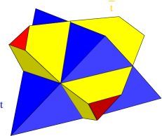
Figure 2. A compound of a tetrahedron $t$ with a truncated tetrahedron $\bar{t}$.

The variables $y_{\tilde{e},\tilde{f}}$ are more interesting and this is the first time that we have encountered them. Using the duality, we can also write them as $y_{e,f}$. There is 12 of them for each tetrahedron. It is natural to interpret them in terms of a certain other truncated tetrahedron. Indeed, let us introduce the dual tetrahedron, and cut off its vertices by surfaces parallel to the faces of $t$ to obtain a truncated tetrahedron $\bar{t}$. A compound object made of $t$ and $\bar{t}$ is shown in Fig. 2. The truncated tetrahedron $\bar{t}$ has 12 vertices, and we shall interpret 12 variables $y_{e,f}$ as describing “positions” of these vertices. The meaning of each $\delta$-function in (6.11) is then as follows: it imposes the constraint that the rotation of a vertex $y_{e,f}$ into $y_{e,f^{\prime}}$ around the edge $e$ is the same as rotation of the face $f$ into $f^{\prime}$ as described by $g$-variables.

Thus, we only have the variables $x_{\tilde{f}}$ uninterpreted. By duality, they are variables $x_{e}$ that have to do with the edges of $t$. Tetrahedron $t$ is truncated, and we interpret $x_{e}$ as describing rotations of the small faces of the truncated tetrahedron $t$ into one another. Thus, interpretation of all of the variables in (6.9) is in terms of geometrical quantities associated with two truncated tetrahedra $t,\bar{t}$ inscribed into one another.

For the convenience of the reader, let us re-write the above edge and vertex factors using the triangulation $\operatorname{{\mathcal{T}}}$ notations. We have:

$$\delta_{e}(\prod_{e}y^{-1}_{e,f}x_{e}^{-1}y_{e,f})$$ (6.12)

for each face $f$ of $\operatorname{{\mathcal{T}}}$. Here the product in the argument of the $\delta$-function is taken over 3 edges that form the boundary of face $f$. The tetrahedron factor is given by:

$$\int\prod_{f}dg^{t}_{f}\prod_{f,f^{\prime}\in t}\,\,\delta_{e}(y_{e,f}g^{t}_{f}(g^{t}_{f^{\prime}})^{-1}y^{-1}_{e,f^{\prime}}).$$ (6.13)

The interpretation that we would like to propose for the total tetrahedron amplitude (6.9) is that of a wave function of a pair of dual to each other truncated tetrahedra. To obtain an amplitude for a manifold one multiplies these wave functions and integrates over the gluing variables $x,y$. We would like to note that there is a similarity in the structure of the vertex found and the expression for the $6j$-symbol obtained in [20]. In both cases the quantity in question has to do with a truncated tetrahedron, and is constructed using propagators for long edges (the second set of $\delta$-functions in (6.9)), and a set of factors for the small faces (the first set of $\delta$-functions in (6.9)). Thus, the structure we have found is probably pertinent to a very general class of models.

If not for the edge factors (6.12), one could easily integrate over the $y$ variables with the result being a product of $\delta$-functions, one for every edge $e$ of $\operatorname{{\mathcal{T}}}$, and requiring that the holonomy around $e$ is trivial. With factors (6.12) the integration is not straightforward. The total amplitude (6.9) is one where tetrahedron constraints discussed in the introduction are taken into account.

6.3. Dual graph analysis

Above we have represented the chain mail evaluation $\Omega CH(D)$ as a composition of vertex kernels (6.9), or the edge (6.10) and vertex (6.11) factors. Edges and vertices are those of $D$. We would now like to group the factors according not to $D$ but to a triangulation $\operatorname{{\mathcal{T}}}$ whose dual graph is $D$.

Thus, Feynman diagrams $D$ have an interpretation of the dual skeleton of some triangulated 3-manifold. Let us denote this triangulation by $\operatorname{{\mathcal{T}}}$. Let us consider vertices $v$ of this triangulation. The edges $e$ of $\operatorname{{\mathcal{T}}}$ are formed by parts of the meridian links of $CH(D)$. The number of strands forming each edge of $\operatorname{{\mathcal{T}}}$ is not fixed, and is equal to the number of faces of $\operatorname{{\mathcal{T}}}$ sharing this edge. Strands forming the edges of Feynman diagram $D$, and whose closure defines the faces of $D$, now enclose the strands forming the edges of $\operatorname{{\mathcal{T}}}$. Thus, we have a very similar structure to that considered above, except that it is a dual one, and that the number of strands enclosed by a link is now not fixed. To evaluate $CH(D)$ we have to insert the identity operator in each strand. Thus, we insert in each edge $e$ of $\operatorname{{\mathcal{T}}}$ the following operator:

$$\delta_{e}(x_{1}^{-1}\ldots x_{n}^{-1})\int dx\,\prod_{i}\delta_{e}(x^{-1}y_{i}).$$ (6.14)

As before, it is convenient to introduce the kernel (6.3):

$$\delta_{e}(y_{1}^{-1}x_{1}^{-1}y_{1}\ldots y_{n}^{-1}x_{n}^{-1}y_{n})\int dx\,\prod_{i}\delta_{x}(y_{i}^{-1}\tilde{y}_{i})\delta_{x_{i}}(\tilde{x}_{i}).$$ (6.15)

As in the previous subsection we can take a composition of such kernels around every vertex of $\operatorname{{\mathcal{T}}}$ by integrating over the $\tilde{x},\tilde{y}$ variables. Taking into account the $\delta_{x_{i}}(\tilde{x}_{i})$ functions, we see that there remains a single variable $x_{f}$ for every face. The $y$-variables can be denoted by $y_{e,f}$. Indeed, there is one such variable for each strand forming each edge of $\operatorname{{\mathcal{T}}}$, or, equivalently, for each face $f$ sharing edge $e$. This vertex kernel is found to be:

$$\prod_{e}\delta_{e}(\prod_{f}y_{e,f}^{-1}x_{f}^{-1}y_{e,f})\prod_{e,e^{\prime}}\delta_{e}(y_{e,f}x_{v,e}x_{v,e^{\prime}}^{-1}y_{e^{\prime},f}^{-1}).$$ (6.16)

Here the second product is over pairs of edges that emanate from $v$, and $f$ in the argument of the second set of $\delta$-functions is the face shared by both $e,e^{\prime}$. Equivalently, one can say that second first product is over the faces that touch $v$. To obtain the chain mail evaluation one should multiply the kernels (6.16) and integrate over all the variables $x_{v,e},x_{f},y_{e,f}$. Note that the vertex (6.16) is essentially the same as (6.9), except that the dual quantities are used.

Let us discuss a geometrical interpretation of the quantities involved in (6.16). The quantity $x_{f}$ is interpreted as the holonomy across the face $f$. The quantity $y_{e,f}$ encodes the dihedral angles of a tetrahedron. Namely, $y_{e,f}y_{e,f^{\prime}}^{-1}$ describes the rotation of face $f$ into $f^{\prime}$ around edge $e$. We see that arguments of the first set of $\delta$-functions in (6.16) are just the product of holonomies across the faces that share $e$ with the group elements that describe rotations of $f$ to the next face $f^{\prime}$. Thus, the argument of the $\delta$-function for edge $e$ is the total rotation that one gets by going around $e$. This means that there is no deficit angle allowed! Thus, in spite of the fact that the model was constructed using $\operatorname{D(SU(2))}$, not just $\operatorname{SU}(2)$, the model does not seem to describe point particles. We shall return to this conundrum below.

For now let us note that an interpretation of the second set of $\delta$-functions in (6.16) is also possible. Indeed, we see that the quantity $x_{v,e}x_{v,e^{\prime}}^{-1}$ describes the rotation of edge $e$ into $e^{\prime}$, with the vertex $v$ as the center of rotation. Each $\delta$-function guarantees that $y_{e,f}^{-1}y_{e^{\prime},f}$ is the same as the rotation that sends $e$ to $e^{\prime}$.

6.4. General models and their point particle interpretation

As we have just seen, the topological GFT model constructed from the identity operator $\delta_{e}(y)$ on the Drinfeld double does not describe point particles. Earlier we have introduced a more general set of models in which a function $\delta_{e}(x)P(y)$ is inserted into the merideans. Now we would like to show that these models do describe point particles and $P(y)$ is the particle’s propagator in the momentum space.

We have seen in the previous subsection, the point particle interpretation, if any, is most visible in a description in which one groups all the projectors around vertices of $\operatorname{{\mathcal{T}}}$. Let us give this description. As before, each edge of $\operatorname{{\mathcal{T}}}$ is formed by a number of strands with the identity operator inserted. However, the operator on the link that encloses the edge is now $P$. Therefore, each edge of $\operatorname{{\mathcal{T}}}$ corresponds to the following operator:

$$P(x_{1}^{-1}\ldots x_{n}^{-1})\prod_{i}\delta_{e}(y_{i}).$$ (6.17)

These operators now have to be multiplied (using the $\bullet$-product) as specified by the fat structure, and the Haar functional has to be applied in each strand to get the amplitude. It is easiest to understand what the result is by noticing that each of these edge operators is actually an element of the ideal $({\mathcal{A}}^{*})^{\otimes n}$. Indeed, functions of the form $f(x)\delta_{e}(y)$ form an ideal in $D(G)$, isomorphic to the algebra ${\mathcal{A}}^{*}$ with point-wise multiplication. Therefore, the result of the $\bullet$-product of all these operators is the point-wise product of the functions $P(x_{1}^{-1}\ldots x_{n}^{-1})$ times the product of the $\delta$-functions $\delta_{e}(y)$. It is now clear what the evaluation is. Let us first discuss what happens with the $y$-dependence. Applying the Haar functional $h$ in each strand we get an infinity $\delta_{e}(e)$. These infinities are cancelled by the prefactor $\eta^{2n_{1}}$ that we introduced in (5.1). One could, actually, avoid this infinities altogether by a slight modification of the evaluation procedure. Thus, since the result in each strand is always in ${\mathcal{A}}^{*}$ ideal of $D(G)$, let us instead of applying the Haar functional of $D(G)$ apply the one of ${\mathcal{A}}^{*}$. The result of this evaluation procedure is finite (for sufficiently nice propagators for which the group integrals would converge).

The result of this evaluation procedure is given by

$$\int\prod_{f}dx_{f}\prod_{e}P(x_{f_{1}}^{-1}\ldots x_{f_{n}}^{-1}).$$ (6.18)

Here the first product is over the faces of the diagram, and $x_{f}$ is a group variable that gets associated to each face. The second product is over the edges of the diagram, and the product of $x$-variables in the argument of the propagator includes these variables for the faces $f_{1},\ldots,f_{n}$ shared by that edge. It is clear now that the function $P(y)$ plays the role of the particle propagator, for the above answer for the amplitude is as expected, see e.g. [1, 2].

Thus, we have arrived at the expression we started from in the Introduction. Indeed, the amplitude is just the Feynman amplitude in the momentum representation, with the propagator evaluated at the product of face variables around an edge. The momentum conservation constraints are solved by introducing the face variables. The tetrahedron constraints that we discussed in the Introduction can be omitted because the integrand is invariant under the action of the gauge transformations at vertices of the dual triangulation, as can be easily checked. Moreover, as the proposition 5.2 states, the Feynman amplitude is to a large extent independent of the extra “fat” structure that is added to the diagram in order to define it.

There are two interesting “limiting cases” to consider. The case $P(y)=\delta_{e}(y)$ corresponds to having no particles at all. This gives the topological Ponzano-Regge model, if one introduces an additional prefactor $\eta^{2n_{3}}$ that is required to guarantee the invariance under the 2-3 moves. The other case is $P(y)=1$, which gives another (trivial) topological model, the one that gives one for every manifold as the amplitude. However, one can decompose the function $P(y)=1$ into $\delta$-functions on conjugacy classes as in (3.25). This shows that even this trivial model can be thought of as containing particles of all possible masses in it, but becoming trivial after the integral over the particles’ mass is taken.

7. Discussion

Let us recap the main points of this work. We have considered the group field theory for the Drinfeld double and constructed an exact analog of the Boulatov model. The Feynman expansion of the model leads to triangulated 3-manifolds weighted with a manifold invariant. The invariant is the “Ponzano-Regge” model for the Drinfeld double. By reducing this Feynman amplitude to the chain mail evaluation we proved that this Drinfeld double Ponzano-Regge amplitude is indeed an invariant of 3-manifolds (when dressed by an appropriate power of the formal quantity $\eta^{2}$). We have also found that this model does not describe point particles. Indeed, one of the factors appearing in the amplitude for this model is a $\delta$-function for the holonomy around each triangulation edge. This is a bit disappointing, because our original motivation for considering the Drinfeld double GFT was precisely to obtain a model containing point particles. Thus, in a certain sense, our original motivation has failed.

Nevertheless, motivated by the GFT considerations, and especially by the chain mail construction, we have introduced a more general set of models that are defined using not GFT but directly in terms of the chain mail. We have considered only one such model, but others are possible. The data that goes into this model is an assignment of a propagator (function on the $\operatorname{SU}(2)$ group manifold) to each edge of the Feynman diagram. This propagator can be chosen different for different edges, as long as it is appropriately normalized. The resulting Feynman amplitude is invariant under moves that do not change the Feynman graph and the 3-manifold topology. This model describes point particles. In fact, it is exactly the naive model envisaged already in the Introduction. Our results on its invariance under the topological moves show that this model is well-defined and to a large extent independent on the “fat” structure that was introduced to define it. The model models become topological if one choses $P(y)=1$. In this case it seems trivial as the amplitude it gives to any manifold is one. At the same time, even in this case the model does describe point particles. One just has to interpret the operator $\hat{1}$ as the integral over particle’s mass, or using physics terminology, the integral over the internal momenta of particles.

The model we have considered (the one constructed with a general propagator $P$ inserted into the longitudes) has an interpretation as describing pure 3d gravity coupled to point particles. As we have discussed in the introduction, there is another possible interpretation. Namely, one can view this model as describing point particles only, but with the backreaction on the metric taken into account. We have not discussed what would be the corresponding theory in the position space. Let us only note that non-commutativity of momentum implies non-commutativity in the position space as well. It would be of interest to formulate point particle theories described here in the position space, and understand what kind of action principle is responsible for them.

Now that one has a model for 3d quantum gravity with point particles, various quantities of physical interest can be computed. However, certain additional developments are necessary in order to achieve this. First it is important to be able to compute not only closed but also open Feynman graph amplitudes. This would give correlation functions. Second and more important, one should find an analog of LSZ reduction formula of field theory that expresses scattering amplitudes in terms of field correlation functions. We shall not attempt this in the present paper.

A remark is in order about the topological invariant defined by our particle model. As we have already mentioned, this is ${\mathcal{Z}}=1$ for any manifold. However, the amplitude for each Feynman diagram (with a fixed set of conjugacy classes $\theta_{e}$ on the edges) is non trivial. Moreover, an amplitude for an open Feynman graph, which describes particle scattering and which we have not considered in this paper is also not trivial, even when one integrates over the internal momenta. This shows that, in spite of seeming triviality, this model is physically interesting.

Let us now return to the topologically invariant model constructed from the identity operator $\delta_{e}(y)$. Several comments are in order. First, it would be interesting to understand how different this model is from that of Ponzano-Regge. The original Ponzano-Regge model imposes the constraints that the holonomy either around edges or dual edges is trivial. The model constructed in this paper imposes both sets of constraints at the same time. For the case of the double of a quantum $\operatorname{SU}_{q}(2)$, which makes the model well-defined (by rendering $\eta^{-2}$ finite), one expects the Drinfeld double “Ponzano-Regge” model to be equal to the usual Ponzano-Regge model amplitude squared. It would be interesting to understand the interpretation of the classical group Drinfeld double case better.

Another remark is that, as is clear from our construction, the gauge symmetry $\delta\phi=\psi,\theta\bullet\psi=0$ of the group field theory is extremely important. From the chain mail description it is clear that topological invariance of the model is intimately related to the fact that $\theta$-projector is used as the propagator of the model. On the other hand, we know that topological invariance of 3d gravity is due to large amount of gauge symmetry present in it. More precisely, diffeomorphisms are so strong in 3d, that they render the theory topological. All this strongly suggests that there is a link between the group field theory and gravity gauge symmetries. In the context of 2d gravity matrix models the relation between gravity and a matrix model is an instance of open-closed string duality, in which one and the same Feynman amplitude has two different interpretations. We expect that the relation between group field theory and 3d gravity explored here is of a similar nature, and that the group field theory gauge symmetry becomes diffeomorphism symmetry on the gravity side. It would be of considerable interest to explore all this in more detail.

It is clear that the GFT construction that we have presented is very general, and can be applied to algebras other than the Drinfeld double. The Drinfeld double of $\operatorname{SU}(2)$ is described [16] as the twisted product of the algebra of functions on $\operatorname{SU}(2)$ with its dual, which is also algebra of functions on $\operatorname{SU}(2)$. The Drinfeld twisted product construction can be applied to groups other than $\operatorname{SU}(2)$. Another important for physical applications example is given by the quantum Lorentz group, which is just the twisted product of the quantum $\operatorname{SU}(2)$ with $q$ real and its Pontryagin dual, see [19]. Our construction can be applied to this case. We expect that in this case there is not one, but several possible models that lead to 3-manifold invariants, depending on which “identity” operator is used. These models should have the physical interpretation as describing point particles coupled to quantum gravity with either positive cosmological constant and Lorentzian signature or with negative cosmological constant and Euclidean signature. It would be of great interest to find all these models.

Appendix: Some useful formulas

In the main text we often use the integral of two and three matrix elements. For two matrix elements we have:

$$\int dg\,\,\overline{T^{j}_{mn}(g)}T^{j^{\prime}}_{m^{\prime}n^{\prime}}(g)=\frac{\delta_{jj^{\prime}}}{{\rm dim}_{j}}\delta_{mm^{\prime}}\delta_{nn^{\prime}}.$$ (7.1)

In graphical notation this takes the following form:

$$\int dg\,\,\,\lower 18.06749pt\hbox{\psfig{height=36.135pt}}=\frac{1}{{\rm dim}}\,\,\lower 18.06749pt\hbox{\psfig{height=36.135pt}}$$ (7.2)

and

$$\int dg\,\,\,\lower 18.06749pt\hbox{\psfig{height=36.135pt}}=\lower 18.06749pt\hbox{\psfig{height=36.135pt}}$$ (7.3)

The intertwiner that is used in the last formula is chosen to be normalized so that:

$$\lower 25.29494pt\hbox{\psfig{height=50.58878pt}}=1$$ (7.4)

whenever the 3 spins satisfy the triangular inequalities, and zero otherwise.

References

- [1] J. W. Barrett, “Feynman diagrams coupled to three-dimensional quantum gravity,” arXiv:gr-qc/0502048.
- [2] L. Freidel and E. R. Livine, “Ponzano-Regge model revisited. III: Feynman diagrams and effective field theory,” arXiv:hep-th/0502106.
- [3] G. Ponzano and T. Regge, “Semiclassical limit of Racah coefficients” in Spectroscopic and group theoretical methods in physics (Bloch ed.), North-Holland, 1968.
- [4] L. Freidel and D. Louapre, “Diffeomorphisms and spin foam models,” Nucl. Phys. B 662, 279 (2003) [arXiv:gr-qc/0212001].
- [5] L. Freidel and S. Majid, “Noncommutative harmonic analysis, sampling theory and the Duflo map in 2+1 quantum gravity,” arXiv:hep-th/0601004.
- [6] L. Freidel and D. Louapre, “Ponzano-Regge model revisited. II: Equivalence with Chern-Simons,” arXiv:gr-qc/0410141.
- [7] J. W. Barrett, J. M. Garcia-Islas and J. F. Martins, “Observables in the Turaev-Viro and Crane-Yetter models,” arXiv:math.qa/0411281.
- [8] D. V. Boulatov, “A Model of three-dimensional lattice gravity,” Mod. Phys. Lett. A 7, 1629 (1992) [arXiv:hep-th/9202074].
- [9] P. H. Ginsparg and G. W. Moore, “Lectures on 2-D gravity and 2-D string theory,” arXiv:hep-th/9304011.
- [10] L. Freidel and D. Louapre, “Non-perturbative summation over 3D discrete topologies,” Phys. Rev. D 68, 104004 (2003) [arXiv:hep-th/0211026].
- [11] F. A. Bais and N. M. Muller, “Topological field theory and the quantum double of SU(2),” Nucl. Phys. B 530, 349 (1998) [arXiv:hep-th/9804130].
- [12] A. Mikovic, “Spin foam models of matter coupled to gravity,” Class. Quant. Grav. 19, 2335 (2002) [arXiv:hep-th/0108099].
- [13] L. Freidel, “Group Field Theory: An overview,” arXiv:hep-th/0505016.
- [14] M. P. Reisenberger and C. Rovelli, “Spacetime as a Feynman diagram: The connection formulation,” Class. Quant. Grav. 18, 121 (2001) [arXiv:gr-qc/0002095].
- [15] R. Dijkgraaf, V. Pasquier and Ph. Roche, “Quasi-Hopf Algebras, Group Cohomology and Orbifold models,” Nucl. Phys. Proc Suppl. 18B, 60-72 (1990)
- [16] T. H. Koornwinder, B. J. Schroers, J. K. Slingerland and F. A. Bais, “Fourier transform and the Verlinde formula for the quantum double of a finite group,” J. Phys. A 32, 8539 (1999) [arXiv:math.qa/9904029].
- [17] J. Roberts, “Skein theory and Turaev-Viro invariants”, Topology 34 771-787 (1995).
- [18] R. De Pietri and C. Petronio, “Feynman diagrams of generalized matrix models and the associated manifolds in dimension 4,” J. Math. Phys. 41, 6671 (2000) [arXiv:gr-qc/0004045].
- [19] S. L. Woronowicz and S. Zakrzewski, “Quantum deformations of the Lorentz group. The *-algebra level”, Compositio Math. 90 211-243 (1994).
- [20] K. Krasnov, “Holography for the Lorentz group Racah coefficients”, Class. Quant. Grav. 22 1933-1944 (2005).