Confining the Electroweak Model to a Brane

Abstract

We introduce a simple scenario where, by starting with a five-dimensional $SU(3)$ gauge theory, we end up with several 4-D parallel branes with localized fermions and gauge fields. Similar to the split fermion scenario, the confinement of fermions is generated by the nontrivial topological solution of a $SU(3)$ scalar field. The 4-D fermions are found to be chiral, and to have interesting properties coming from their 5-D group representation structure. The gauge fields, on the other hand, are localized by loop corrections taking place at the branes produced by the fermions. We show that these two confining mechanisms can be put together to reproduce the basic structure of the electroweak model for both leptons and quarks. A few important results are: Gauge and Higgs fields are unified at the 5-D level; and new fields are predicted: One left-handed neutrino with zero-hypercharge, and one massive vector field coupling together the new neutrino with other left-handed leptons. The hierarchy problem is also addressed.

I Introduction

One of the most remarkable twists that the braneworld scenario has introduced in our view of physics is that the fundamental scale of gravity could be significantly closer to scales currently accessible by experiments than previously thought. In the braneworld paradigm, the standard model of physics is localized to a four dimensional brane while gravity (and possibly other fields) propagate in the entire space, the bulk. In the 4-D perspective, this results in the rescaling of many couplings and mass scales present in the theory, thus providing an alternative approach to the hierarchy problem Ant ; Ant2 ; Ant3 ; Ant4 ; TeV1 ; TeV2 . Naturally, an important problem in the study of this type of theories is understanding the possible ways in which the standard model can be localized to a brane Rev1 ; Rev2 ; different mechanisms to localize matter and gauge fields to a brane may have distinctive features with relevant implications for braneworld phenomenology. In addition, several aspects of the standard model’s rich structure could be understood in terms of how physics is arranged in the bulk.

A simple mechanism for the confinement of higher dimensional fermions to a domain wall was proposed long ago by Rubakov and Shaposhnikov fermions1 and is based purely on field theoretical considerations. In their proposal, the wave functions of fermion zero modes concentrate near the existing domain walls, generating 4-D massless chiral fermions attached to them. This mechanism has given rise to interesting braneworld scenarios with clear consequences for physics beyond the standard model. One is the split fermion scenario, proposed by Arkani-Hamed and Schmaltz fermions2 . Here, bulk fermions are split into different positions around the brane, offering a simple solution to the hierarchy problem and the proton decay problem: the separation between chiral fermions along the extra dimension generates exponentially suppressed couplings between them (for example, Yukawa couplings) fermions3 ; fermions4 .

In the case of gauge fields, a mechanism for their localization (closely related to the confinement of fermions) is also available. This is the case of the quasilocalization of gauge fields, proposed by Dvali, Gabadadze and Shifman gauge (see alt1 ; alt2 for alternatives). Here, the interaction between bulk gauge fields and the “already” localized fermions induces gauge kinetic terms on the brane. The result is a 4-D effective theory consisting of gauge fields mediating interactions between the localized fermions. An interesting feature of this type of mechanism is the appearance of a crossover scale $r_{c}$: at distances below this scale the propagation of gauge fields along the brane is manifestly four-dimensional, whereas above this scale the propagation becomes five-dimensional.

In this paper we put together both types of confining mechanisms —for fermions and gauge fields— to reproduce the basic structure of the electroweak sector of the standard model. We show that the gauge symmetry exhibited by bulk fermions can be broken down through their confinement to a domain wall, giving rise to non-trivial subgroup representations. More precisely, by starting with a five-dimensional $SU(3)$ gauge theory in the bulk, we obtain an $SU(2)\times U(1)$ chiral theory on the brane, with all the basic requirements of the electroweak model.

The key ingredient of the present proposal is that the positions at which 5-D fermions end up localized depend on their $SU(3)$ charges. This allows, for example, to break the $\mathbf{10}$ and $\bar{\mathbf{6}}$ representations of $SU(3)$ down to the lepton and quark representations of $SU(2)\times U(1)$, respectively, and confine them to a single brane. In this construction it is possible to identify the Higgs field with the fifth component of the localized bulk gauge field. Additionally, new fields inevitably appear in the resulting 4-D effective theory. These are: a left-handed neutrino with zero-hypercharge, and a massive vector field coupling together the new neutrino with other left-handed leptons.

This article is organized as follows: In Sec. II we introduce the split fermion scenario and explain how the localization of $SU(3)$ fermions to different positions in the bulk is produced. Then, in Sec. III we analyze the confinement of gauge fields. There we argue that the gauge symmetry of the localized fermions is transferred to the gauge fields near the brane. Finally, in Sec. IV, we show that the electroweak model can be constructed by putting these two mechanisms together. There, the hierarchy problem is also addressed.

II Confinement of fermions

In this section we describe the localization of bulk fermions to a domain wall. We start with the split fermion scenario and then move to a more complex setup where the localization of fermions depends on their charges.

II.1 Split fermions

Consider a 5-D system consisting of a spin-1/2 fermion $\Psi$ and a real scalar field $\Phi$. To describe the 5-D space-time we use coordinates $x^{A}$ with $A=1,\ldots,5$. The Lagrangian for the system is

$$\mathcal{L}^{(5)}=-\bar{\Psi}\left[\gamma^{A}\partial_{A}+m+y\,\Phi\right]\Psi-\frac{1}{2}(\partial_{A}\Phi)^{2}-V(\Phi).$$

(1)

Here $m$ is the mass of the bulk fermion $\Psi$ and $y$ is a Yukawa coupling. Additionally, $\gamma^{A}$ are the 5-D gamma-matrices in a basis where

$$\gamma^{5}=\left(\begin{array}[]{cc}1&0\\ 0&-1\end{array}\right),$$ (4)

which is the usual four-dimensional $\gamma^{5}$ matrix. For the time being we disregard the presence of gauge fields. Let us consider the following potential for the scalar $\Phi$:

$$V(\Phi)=\frac{\sigma}{4}\left[\Phi^{2}-v^{2}\right]^{2}.$$ (5)

To discuss solutions to this system we use $z=x^{5}$ to distinguish the extra-dimension and coordinates $x^{\mu}$ with $\mu=1,\cdots,4$ to parameterize the usual 4-D space-time. Then, the scalar field $\Phi$ is found to have a kink solution of the form:

$$\Phi(z)=v\tanh\left(kz\right),$$ (6)

where $k=v\sqrt{\sigma/2}\,$. The corresponding domain wall, centered at $z=0$, is coupled to the fermion field through the $y$-term. The equation of motion for $\Psi$ reads:

$$\left[\gamma^{\mu}\partial_{\mu}+\gamma^{5}\partial_{z}+m+y\,\Phi(z)\right]\Psi=0.$$ (7)

Notice that the translational invariance along $z$ is broken. Thus, in order to solve Eq. (7) we define left and right handed helicities $\Psi_{L}$ and $\Psi_{R}$, by $\gamma^{5}\Psi_{L}=+\Psi_{L}$ and $\gamma^{5}\Psi_{R}=-\Psi_{R}$, and expand them as:

$$\Psi_{L,R}=\sum_{n}\Psi^{n}_{L,R}=\sum_{n}a^{L,R}_{n}(z)\,\psi_{L,R}^{n}(x),$$ (8)

where $a_{n}^{L,R}(z)$ are Kaluza-Klein coefficients, $\psi^{n}_{L,R}(x)$ are 4-D left and right-handed spinor fields, and $n$ labels the expansion mode. Inserting the expansion (8) back into Eq. (7) we find the following equations for the coefficients $a_{0}(z)$ and $a_{n}(z)$ with $n>0$:

$$\left[\pm\partial_{z}+m+y\,\Phi\right]a_{0}^{L,R}=0,$$ (9)

$$\left[-\partial_{z}^{2}+(m+y\,\Phi)^{2}\mp y\,(\partial_{z}\Phi)\right]a_{n}^{L,R}=\mu_{n}^{2}a_{n}^{L,R},$$ (10)

where $\pm$ stands for the left and right-handed helicities. At this stage, it is convenient to define the following “confinement” length scale:

$$\Delta=\frac{1}{\sqrt{|yvk|}}.$$ (11)

Then, in general, solutions to Eq. (10) provide modes with masses $\mu_{n}^{2}$ of order $\Delta^{-2}$. From now on we assume that $\Delta$ is sufficiently small so that nonzero modes can be integrated out without affecting the theory at low energies. Solving Eq. (9) the zero modes are found to be

$$\Psi_{L,R}=A\exp\Big{\{}\mp\!\int^{z}_{0}\!\!\!\left[m+y\,\Phi(z)\right]\,dz\Big{\}}\,\psi_{L,R}(x),$$ (12)

where the factor $A$ is a normalization constant introduced in such a way that

$$\int dz\,|\Psi|^{2}=|\psi(x)|^{2}.$$ (13)

Notice that only one of these two solutions is normalizable: if $y>0$ ($y<0$) then the left (right) handed fermion is normalizable. Additionally, observe that if $m=0$ then the fermion wave function is centered at $z=0$, otherwise its localization is shifted with respect to the brane. To appreciate this, let us analyze the linear behavior $\Phi\simeq vkz$ near $z=0$ for the case $y>0$. Then, if we assume that $m^{-1}\gg k\Delta^{2}$ (so the linear expansion $\Phi\simeq vkz$ makes sense), we obtain

$$\Psi_{L}\sim\frac{1}{\sqrt{\Delta}}\exp\left[-\frac{1}{2}\Delta^{-2}(z-z_{0})^{2}\right]\,\psi_{L}(x),$$ (14)

where $z_{0}=-m\Delta^{2}$. Thus, the fermion wave function has a width $\Delta$ and is centered at $z_{0}$. Figure 1 sketches the confinement of the bulk fermion near the domain wall.

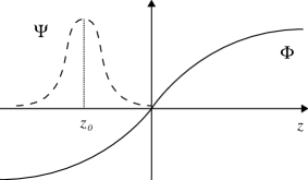
Figure 1: The figure sketches the confinement of the bulk fermion near the domain wall located at $z=0$. The fermion wave function is centered at position $z_{0}=-m\Delta^{2}$.

We can now compute the 4-D effective Lagrangian for $\psi_{L}(x)$ by integrating out the extra-dimension:

$$\mathcal{L}^{(4)}=-\bar{\psi}_{L}(\gamma^{\mu}\partial_{\mu})\psi_{L}.$$ (15)

Notice that in the limit $\Delta\rightarrow 0$ ($z_{0}\rightarrow 0$), we obtain a thin brane of the form:

$$\mathcal{L}^{(5)}=\delta(z)\mathcal{L}^{(4)}.$$ (16)

There is an interesting consequence related to the shift of the fermion’s positions with respect to the domain wall: Suppose a scenario in which two bulk fermions $\Psi^{1}$ and $\Psi^{2}$, with masses $m_{1}$ and $m_{2}$, are coupled to a wall in such a way that $y_{1}=y>0$ and $y_{2}=-y<0$. If in the original 5-D Lagrangian there is a term such as

$$H\bar{\Psi}^{1}\Psi^{2}+\mathrm{h.c.},$$ (17)

where $H$ is a given bulk field (a scalar, for example), then the 4-D effective Lagrangian will contain a Yukawa term of the form:

$$\sim(H\,\bar{\psi}^{1}_{L}\,\psi^{2}_{R}+\mathrm{h.c.})\,e^{-r^{2}/4\Delta^{2}},$$ (18)

where $r=r_{1}-r_{2}$ is the separation between both fermion wave functions with $r_{1}=-m_{1}\Delta^{2}$ and $r_{2}=+m_{2}\Delta^{2}$. Physically, this means an exponential suppression of the 4-D Yukawa coupling for the pair ($\psi^{1}_{L}$, $\psi^{2}_{R}$) offering an interesting solution to the hierarchy problem.

II.2 Confining $SU(3)$ fermions

We now proceed to analyze the localization of fermions produced by “charged” domain walls. Assume that space-time is described by a 5-D manifold $M$ with topology

$$M=\mathbb{R}^{4}\times S^{1},$$ (19)

where $S^{1}$ is the one-dimensional circle and $\mathbb{R}^{4}$ is the 4-D Lorentzian space. In this case, the coordinate $z=x^{5}\in[0,L]$ is the spatial coordinate parameterizing $S^{1}$ with $L$ the size of the compact extra-dimension. Let us consider the existence of 5-D bulk fermions transforming nontrivially under $SU(3)$ gauge symmetry. They are described by the following Lagrangian:

$$\mathcal{L}_{\Psi}^{(5)}=-\bar{\Psi}[\gamma^{A}D_{A}+Y(\Phi)]\Psi.$$ (20)

The covariant derivative is $D_{A}\Psi=(\partial_{A}-iE^{\alpha}_{A}T_{\alpha})\Psi$, where $E^{\alpha}_{A}$ are $SU(3)$ bulk gauge fields. Here $\alpha=1,\ldots,8$ and $T_{\alpha}$ are the $SU(3)$ generators acting on $\Psi$. Observe that we are considering a coupling term $Y(\Phi)$ where $\Phi=\Phi^{\alpha}T_{\alpha}$ is a scalar field that transforms in the adjoint representation of $SU(3)$. In order to construct $SU(3)$-representations we proceed conventionally: We choose $T_{3}$ and $T_{8}$ as the Cartan generators and construct states to be eigenvalues with charges:

$$Q=(T_{3},T_{8}).$$ (21)

Assume that $\Phi$ is dominated by the following $SU(3)$ gauge invariant potential:

$$V(\Phi)=\frac{\sigma}{4}\left[\Phi^{\alpha}\Phi_{\alpha}-v^{2}\right]^{2}.$$ (22)

Nonzero vacuum expectation solutions $\langle\Phi\rangle$ are expected and, in general, they correspond to linear combinations of $\langle\Phi^{3}\rangle$ and $\langle\Phi^{8}\rangle$. Furthermore, since we are assuming the compact topology (19), then the system admits nontrivial topological solutions. Take for instance the case of a single winding-number solution

$$\langle\Phi(z)\rangle=\Phi_{0}\left[\cos(kz)T_{3}+\sin(kz)T_{8}\right],$$ (23)

where $k=2\pi/L$ and $\Phi_{0}^{2}=v^{2}-k^{2}/\sigma$. Notice that we have chosen $\langle\Phi^{8}\rangle=0$ at $z=0$. We can now proceed in the same way as before: we expand $\Psi$ in modes (8) and find zero mode solutions of the form

$$\Psi_{L,R}=A\exp\left\{\mp\int^{z}_{0}\!\!\!Y(z)\,dz\right\}\,\psi_{L,R}(x),$$ (24)

where $Y(z)\equiv Y[\langle\Phi(z)\rangle]$. To discuss the consequences of solution (23) with some transparency, let us have a look to the following simple example: take a Yukawa coupling of the form:

$$Y(\Phi)=y\Phi=y\Phi^{\alpha}T_{\alpha},$$ (25)

and consider matter fields $\Psi$ belonging to the $\mathbf{3}$ [the fundamental representation of $SU(3)$]. In this case the confinement scale must be defined as

$$\Delta=\frac{1}{\sqrt{|y\Phi_{0}k|}}.$$ (26)

Thus again, masses $\mu_{n}^{2}$ of nonzero modes solutions [Eq. (10)] are found to be of order $\Delta^{-2}$.

To work out the consequences of the Yukawa coupling (25) on the $\mathbf{3}$ we chose $\Psi^{i}$ (with $i=1,2,3$) to have the following $SU(3)$-charges (see Fig. 2):

$$Q(\Psi^{1}) = (-1/2,+\sqrt{3}/6),$$ (27)

$$Q(\Psi^{2}) = (+1/2,+\sqrt{3}/6),$$ (28)

$$Q(\Psi^{3}) = (0,-\sqrt{3}/3).$$ (29)

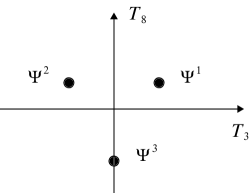
Figure 2: The figure shows the $SU(3)$-charges, $T_{3}$ and $T_{8}$, of fermions $\Psi^{i}$ (with $i=1,2,3$) in the fundamental representation $\mathbf{3}$.

In this way, replacing (25) into (24), it is possible to see that the positions at which the fermion wave functions end up centered depend on their $SU(3)$-charges and their chirality. Observe, for instance, that in the present realization left and right-handed fermions are localized to diametrically opposite positions in the $S^{1}$ circle. Also, it can be seen that if $|y\Phi_{0}|\gg k$, then the widths of the fermion wave functions become of order $\Delta$ and the overlap between fermions located at different positions becomes very small. The following table provides the position of each state for the case $y\Phi_{0}>0$:

Fermion		Position ($z$)	Fermion		Position ($z$)
$\Psi^{3}_{R}$		0	$\Psi^{3}_{L}$		L/2
$\Psi^{1}_{R}$		2L/3	$\Psi^{1}_{L}$		L/6
$\Psi^{2}_{R}$		5L/6	$\Psi^{2}_{L}$		L/3

Notice that the fundamental representation has been broken down to several branes. Figure 3 shows the way in which $\Psi^{3}$ of the fundamental representation is split.

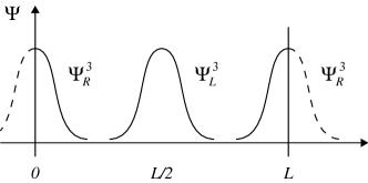
Figure 3: The figure shows the way in which $\Psi^{3}$ is confined. Same representations but with different chiralities end up in branes located at diametrically opposite positions in the $S^{1}$ circle.

We can now compute the 4-D effective theory for the matter fields localized at any desired brane of our example. Let us compute, for instance, the effective Lagrangian $\mathcal{L}_{\mathrm{eff}}$ at the first brane ($z=0$) taking into account the presence of the gauge field $E^{\alpha}_{A}$. In the limit $\Delta\rightarrow 0$ (with $L$ fixed), we obtain:

$$\mathcal{L}_{\mathrm{eff}}=-\delta(z)\bar{\psi}^{3}_{R}\gamma^{\mu}\bigg{[}\partial_{\mu}+i\frac{\sqrt{3}}{3}E^{8}_{\mu}\bigg{]}\psi^{3}_{R}.$$ (30)

Here the delta function appears in the limit $\Delta\rightarrow 0$ after considering the right normalization factor $A$ in Eq. (24). Notice the appearance of the induced current

$$J_{8}^{\mu}=-i\frac{\sqrt{3}}{3}\bar{\psi}^{3}_{R}\gamma^{\mu}\psi^{3}_{R},$$ (31)

which couples to the gauge field component $E^{8}_{\mu}$ in (30). The appearance of such currents will be important to understand the localization of gauge fields (Sec. II.3).

II.3 Generalization of the mechanism

In general, given a nonzero v.e.v for a scalar field $\Phi(z)$, the position $z$ at which the fermion wave function $\Psi$ is centered is determined by the condition

$$Y(z)\,\Psi=0,$$ (32)

where $Y(z)=Y[\Phi(z)]$. The chirality of such a state is determined by the sign of the derivative $\partial_{z}Y(\Phi)$ at the given position. To be more precise, if $\partial_{z}Y(\Phi)>0$ ($\partial_{z}Y(\Phi)<0$), then the confined fermion is left (right) handed.

III Localization of gauge fields

We now focus on the gauge sector of the model. The localization of gauge fields to domain-walls is ensured by the already localized fermionic fields; this is the case of the quasilocalization of gauge fields gauge . The interaction between the localized currents at the branes with the 5-D gauge fields induces an effective 4-D theory in the brane. This is produced by one-loop contributions to the effective action coming from the brane currents.

III.1 Quasi-localization of gauge fields

For simplicity, we focus only on the localization of gauge fields to the first brane ($z=0$) and neglect the effect of the coupling between $E^{\alpha}_{A}$ and $\Phi$ on the 5-D behavior of $E^{\alpha}_{A}$ near the brane. Now, assume that the spinor fields are already confined and that the overlap between different branes is very small ($\Delta^{-1}\gg k$). Then, in general, the Lagrangian for the gauge fields $E^{\alpha}_{A}$ about the brane at $z=0$ is given by

$$\mathcal{L}^{(5)}_{\mathrm{G}}=-\frac{1}{4g^{2}}F^{\alpha}_{AB}F_{\alpha}^{AB}+\delta(z)E^{\alpha}_{A}J_{\alpha}^{A}(x),$$ (33)

where $F^{\alpha}_{AB}=\partial_{A}E^{\alpha}_{B}-\partial_{B}E^{\alpha}_{A}+C^{\alpha}_{\beta\gamma}E^{\beta}_{A}E^{\gamma}_{B}$ (here $C^{\alpha}_{\beta\gamma}$ are the $SU(3)$ structure constants) and $g$ is the gauge coupling. As mentioned, the currents $J^{A}_{\alpha}(x)$, localized at the branes, appear as a consequence of the covariant derivative $D_{A}\Psi=(\partial_{A}-iE_{A}^{\alpha}T_{\alpha})\Psi$. To continue, it is important to observe that, in general, the currents $J^{A}_{\alpha}(x)$ do not continue transforming covariantly under the full set of gauge symmetry transformations [as in Eq. (30)]. This is because the many components of the $SU(3)$-spinor representations end up at different positions along the fifth dimension. In fact: since the effective terms for gauge fields are induced by loops from these currents, then the transformation properties of $J^{A}_{\alpha}(x)$ will be transferred to the confined gauge fields. Take, for instance, the case of our previous example in which the 4-D effective theory is given by Eq. (30). There, $\psi^{3}_{R}$ provides the current $J_{8}^{\mu}=-i\frac{\sqrt{3}}{3}\bar{\psi}^{3}_{R}\gamma^{\mu}\psi^{3}_{R}$ which couples only to $E^{8}_{\mu}$. Then, a one-loop correction induces the following Lagrangian for $E^{8}_{\mu}$ at the brane:

$$\mathcal{L}^{(4)}=-\frac{1}{4\lambda^{2}}(\partial_{\mu}E^{8}_{\nu}-\partial_{\nu}E^{8}_{\mu})^{2},$$ (34)

where

$$\lambda^{-2}=\frac{N}{12\pi^{2}}\ln(\Lambda/\mu).$$ (35)

Here, $\Lambda$ and $\mu$ are the ultraviolet and infrared cut-offs scales of the 5-D theory and $N=1/3$ (which comes from the coefficient $\sqrt{3}/3$ in $J_{8}^{\mu}$).

III.2 Localization of $SU(2)\times U(1)$ gauge fields

Let us now specialize to the case in which the localized currents preserve the $SU(2)\times U(1)$ transformation properties at the first brane $z=0$. Then it makes sense to perform the following decomposition of the five-dimensional $SU(3)$ gauge field $E^{\alpha}_{A}$:

$$W_{\mu}^{a} = E_{\mu}^{a}\qquad\mathrm{with}\qquad a=1,2,3,$$ (36)

$$V_{\mu}^{i} = E_{\mu}^{i}\qquad\mathrm{with}\qquad i=4,5,6,7,$$ (37)

$$\phi^{i} = E_{5}^{i}\qquad\mathrm{with}\qquad i=4,5,6,7,$$ (38)

$$B_{\mu} = E_{\mu}^{8}.$$ (39)

In the limit $\Delta\rightarrow 0$, other components of $E_{A}^{\alpha}$ are decoupled from the matter fields confined to the branes (this is because these components are coupling together spinor fields with different chiralities that necessarily end up at different branes). In this decomposition, the only non-zero structure constant are: $C_{ab}^{c}$, $C_{ij}^{a}$ and $C_{ij}^{8}$ (and obvious permutation of indices). Then, the current term can be expressed as

$$E^{\alpha}_{A}J^{A}_{\alpha}=W^{a}_{\mu}J_{a}^{\mu}(x)+B_{\mu}J^{\mu}(x)+V^{i}_{\mu}J_{i}^{\mu}(x)+\phi^{i}J_{i}(x),$$

and the 4-D induced action for the now localized fields $W_{\mu}^{a}$, $V_{\mu}^{i}$, $B_{\mu}$ and $\phi^{i}$ at the first brane ($z=0$) becomes

$$\mathcal{L}^{(4)}_{\mathrm{G}} = -\frac{1}{4\lambda^{2}_{H}}H^{a}_{\mu\nu}H_{a}^{\mu\nu}-\frac{1}{4\lambda^{2}_{G}}G_{\mu\nu}G^{\mu\nu}$$ (41)

$$-\frac{1}{2\lambda^{2}_{\phi}}|D\phi|^{2}-\frac{1}{4\lambda^{2}_{Q}}Q^{i}_{\mu\nu}Q_{i}^{\mu\nu}+\mathcal{L}_{V}.\qquad$$

Here $H_{\mu\nu}^{a}$, $Q_{\mu\nu}^{i}$, $G_{\mu\nu}$ and $D_{\mu}\phi^{i}$ are defined as

$$H_{\mu\nu}^{a} = \partial_{\mu}W_{\nu}^{a}-\partial_{\nu}W_{\mu}^{a}+C^{a}_{bc}W_{\mu}^{b}W_{\nu}^{c},$$

$$Q_{\mu\nu}^{i} = \partial_{\mu}V_{\nu}^{i}-\partial_{\nu}V_{\mu}^{i}+C^{i}_{aj}W_{\mu}^{a}V_{\nu}^{j}+C^{i}_{ja}V_{\mu}^{j}W_{\nu}^{a}$$

$$+C^{i}_{8j}B_{\mu}V_{\nu}^{j}+C^{i}_{j8}V_{\mu}^{j}B_{\nu},$$

$$G_{\mu\nu} = \partial_{\mu}B_{\nu}-\partial_{\nu}B_{\mu},$$

$$D_{\mu}\phi^{i} = \partial_{\mu}\phi^{i}+C^{i}_{aj}W^{a}_{\mu}\phi^{j}+C^{i}_{8j}B_{\mu}\phi^{j}.$$ (42)

Additionally, in Eq. (41) we have introduced $\mathcal{L}_{V}$ which contains interaction terms between the vector field $V_{\mu}^{i}$ and the rest of the induced fields

$$\mathcal{L}_{V}=-\frac{1}{4\lambda^{2}_{1}}\left(R_{\mu\nu}^{a}R^{\mu\nu}_{a}+K_{\mu\nu}K^{\mu\nu}\right)-\frac{1}{2\lambda^{2}_{2}}H^{a}_{\mu\nu}R^{\mu\nu}_{a}$$

$$-\frac{1}{2\lambda^{2}_{3}}G_{\mu\nu}K^{\mu\nu}-\frac{1}{2\lambda^{2}_{4}}\left(S_{\mu}^{a}S^{\mu}_{a}+S_{\mu}S^{\mu}\right),\qquad$$ (43)

where we have defined: $R_{\mu\nu}^{a}=C^{a}_{ij}V_{\mu}^{i}V_{\nu}^{j}$, $S_{\mu}^{a}=C^{a}_{ij}V_{\mu}^{i}\phi^{j}$, $S_{\mu}=C_{ij}^{8}V^{i}_{\mu}\phi^{j}/\sqrt{3}$ and $K_{\mu\nu}=C^{8}_{ij}V_{\mu}^{i}V_{\nu}^{j}/\sqrt{3}$. Finally, the various couplings $\lambda_{H}$, $\lambda_{G}$, $\lambda_{Q}$ and $\lambda_{\phi}$ in (41), and $\lambda_{1}$, $\lambda_{2}$, $\lambda_{3}$ and $\lambda_{4}$ in (43) are, in general, found to be of the form

$$\frac{1}{\lambda^{2}}=\frac{N}{12\pi^{2}}\ln\frac{\Lambda}{\mu},$$ (44)

where $N$ measures the number of fermions present in the different loops, taking also into account the values of the various $SU(3)$-charges and combinatorics. For example, we have

$$N_{H}=\mathrm{Tr}\left(T_{3}^{2}\right),\quad\mathrm{and}\quad N_{G}=\mathrm{Tr}\left(T_{8}^{2}\right),$$ (45)

where the traces run over all charged fermions taking place in the loops inducing the first and second terms of (41). Notice, however, that the values of the $\lambda$-couplings may change when taking into account the split of fermions. For instance, as we shall see in Sec. IV.4, the $Y$ coupling of Eq. (20) could induce the split of fermions around a single brane (for example, the first brane at $z=0$). This would result in a modification of the way in which the induced 4-D effective theory is computed, and therefore the way $N$ is computed in (44). Nevertheless, the values of the $\lambda$-couplings should all remain of the same order.

III.3 Gauge theory near the brane

The complete action describing the behavior of the gauge field $E_{A}^{\alpha}$ near the first brane now consists of:

$$\mathcal{L}^{(5)}_{\mathrm{G}}=-\frac{1}{4g^{2}}F^{\alpha}_{AB}F_{\alpha}^{AB}+\delta(z)\mathcal{L}^{(4)}_{\mathrm{G}},$$ (46)

where $\mathcal{L}^{(4)}_{\mathrm{G}}$ is the induced Lagrangian (41). To study the propagation of gauge fields on the braneworld it is convenient to define a crossover scale $r_{c}=g^{2}/2\lambda^{2}$. Then, the physics taking place at the brane can be shown to have two different regimes gauge : at large distances $r\gg r_{c}$ the propagator of the gauge fields becomes five-dimensional, whereas at short distances $r\ll r_{c}$ it becomes four-dimensional.

IV Confining the electroweak model to a brane

We now turn to the confinement of the electroweak model. Our approach consists of adding a new scalar field into the model so as to allow a richer structure to the localization mechanism generated by the $Y$-coupling. Then we show that leptons can be obtained from the $\mathbf{10}$-representation of $SU(3)$, while quarks can be obtained from the $\mathbf{\bar{6}}$.

IV.1 Construction of the Electroweak brane

To start, assume the existence of the same scalar field $\Phi=\Phi^{\alpha}T_{\alpha}$ (as discussed previously) and an additional scalar field $\Theta=\Theta^{\alpha}T_{\alpha}$ also transforming in the adjoint representation of $SU(3)$. This scalar is dominated by the following $SU(3)$ gauge invariant potential:

$$U\propto\left[\Theta^{\alpha}\Theta_{\alpha}-u^{2}\right]^{2},$$ (47)

where $u$ is a constant parameter of the theory. Now, consider the following $Y$-coupling:

$$Y=-y\left(\frac{1}{2}\{\Phi,\Theta\}-\frac{1}{4}\Theta^{\alpha}\Phi_{\alpha}+p\frac{\sqrt{3}}{2}u\,\Phi\right),$$ (48)

where $\{\,,\}$ denotes anticommutation. In the previous equation, $p$ is a parameter of the model that depends on the representation on which $Y$ is acting; in the present construction we allow the value $p=1$ if $Y$ couples to the $\mathbf{10}$, and $p=-1/3$ if $Y$ couples to the $\mathbf{\bar{6}}$. Other gauge invariant terms can also be included in (48) without modifying the main results of this section (we come back to this point towards the end of this section).

We now focus on the case in which $\Theta$ acquires the following v.e.v.:

$$\langle\Theta\rangle=u\,T_{8}.$$ (49)

Then, after the scalars have acquired their respective v.e.v.’s we are left with the following $z$-dependent coupling:

$$(y\Phi_{0}u)^{-1}Y = -\left[(T_{8}+p\sqrt{3}/2)T_{8}-1/4\right]\sin(kz)$$ (50)

$$-\left[T_{8}+p\sqrt{3}/2\right]T_{3}\cos(kz).$$

Similar to our previous example, in this case the widths of the fermion wave functions become of order $\Delta$ (the confining length scale) which now is found to be

$$\Delta=\frac{1}{\sqrt{|y\Phi_{0}|uk}}.$$ (51)

In what follows we analyze separately the confinement of leptons (from the $\mathbf{10}$) and quarks (from the $\mathbf{\bar{6}}$).

IV.2 Leptons

Here we study the action of $Y$ on the $\mathbf{10}$ (where $p=1$) and show that the confined fermions to the domain wall can be identified with the usual leptons of the electroweak model.

IV.2.1 Confining leptons

To proceed it is convenient to consider the decomposition of $SU(3)$ into $SU(2)$ subgroups (see Fig. 4). The $\mathbf{10}$ has the following decomposition: $\mathbf{10}=\mathbf{1}\oplus\mathbf{2}\oplus\mathbf{3}\oplus\mathbf{4}$, with the following $T_{8}$-charges: $T_{8}=-\sqrt{3},-\sqrt{3}/2,\,0,+\sqrt{3}/2$.

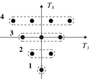
Figure 4: The figure shows the $\mathbf{10}$ representation and its decomposition into $SU(2)$ subgroups: this is $\mathbf{10}=\mathbf{1}\oplus\mathbf{2}\oplus\mathbf{3}\oplus\mathbf{4}$ with charges $T_{8}=-\sqrt{3},-\sqrt{3}/2,\,0,+\sqrt{3}/2$, respectively.

Using this notation, we can work out the localization produced by the $Y$-coupling to the first brane at $z=0$. First, observe from Eq. (50) that all of those states in the $\mathbf{10}$ with $(T_{8}+\sqrt{3}/2)T_{3}=0$ give $Y=0$ at $z=0$. Then, following the reasoning of Sec. II.3, a chiral fermion from each one of these states will confine to $z=0$. The precise chirality of each state depends on the sign of $\partial_{z}Y(z)$. In the present case, assuming $y>0$, the confined states are: the right-handed $SU(2)$-singlet $R\equiv\psi^{\mathbf{1}}_{R}$ with charge $Q=(0,-\sqrt{3})$; the two left-handed components of the $SU(2)$-doublet $L\equiv\psi^{\mathbf{2}}_{L}$ with charges $Q=(-1/2,-\sqrt{3}/2)$ and $Q=(+1/2,-\sqrt{3}/2)$; and only one left-handed component from the triplet $N\equiv\psi^{\mathbf{3}}_{L}$, with charge $Q=(0,0)$. States with opposite chirality are confined to a “mirror-brane” located at $z=L/2$, and any other states are confined elsewhere. Figure 5 shows those components of the $\mathbf{10}$ that confine to $z=0$.

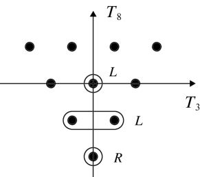
Figure 5: The figure shows those states of the $\mathbf{10}$ that end up localized to $z=0$. The labels $L$ and $R$ indicate the chirality of the confined states.

Now, the 4-D effective Lagrangian for the massless leptons at the first brane is found to be

$$\mathcal{L}_{\mathrm{lep}}^{(4)} = -\bar{L}\Big{[}\gamma^{\mu}\partial_{\mu}-i\gamma^{\mu}W^{a}_{\mu}T_{a}+i\frac{\sqrt{3}}{2}\gamma^{\mu}B_{\mu}\Big{]}L$$

$$-\bar{R}\Big{[}\gamma^{\mu}\partial_{\mu}+i\sqrt{3}\gamma^{\mu}B_{\mu}\Big{]}R-\bar{N}\gamma^{\mu}\partial_{\mu}N+\mathcal{L}_{\mathrm{I}}^{(4)},$$

where $\mathcal{L}_{\mathrm{I}}^{(4)}$ contains interaction terms involving $\phi^{i}$ and $V^{i}_{\mu}$

$$\mathcal{L}_{\mathrm{I}}^{(4)}=-i\alpha\,\phi^{i}\bar{R}\,T_{i}\,L-i\beta\,V^{i}_{\mu}\bar{N}\gamma^{\mu}\,T_{i}\,L+\mathrm{h.c.},$$ (53)

where $\alpha$ and $\beta$ are coefficients that appear from the overlap between wave functions of different widths. In the present case, $\alpha=\beta=(5)^{1/4}/\sqrt{3}$. In Eqs. (LABEL:eq:_leptons) and (53), $T_{a}$ and $T_{i}$ denote the action of the corresponding $SU(3)$-generators on the $SU(2)$-doublet $L=\psi^{\mathbf{2}}_{L}$. We can rewrite the $T_{i}$’s in Eq. (53) to obtain a more transparent notation

$$\mathcal{L}_{\mathrm{I}}^{(4)}=-i\alpha\frac{\sqrt{3}}{2}\phi^{i}\bar{R}\,t_{i}\,L-i\beta V^{i}_{\mu}\bar{N}\gamma^{\mu}\,s_{i}\,L+\mathrm{h.c.},$$ (54)

where $t_{i}$ and $s_{i}$ with $i=4,5,6,7$, are $1\times 2$ matrices acting on $L$ given by

$$t_{4}=s_{6}=(1,0), \qquad t_{5}=-s_{7}=i(1,0),$$

$$t_{6}=s_{4}=(0,1), \qquad t_{7}=-s_{5}=i(0,1).$$ (55)

IV.2.2 Confining gauge fields

The form of the theory presented in Eqs. (LABEL:eq:_leptons) and (53) corresponds to an $SU(2)\times U(1)$ gauge theory with four massless chiral states. Therefore we can deduce the quasilocalization of gauge fields to the first brane as discussed in Sec. III [with the same Lagrangian shown in (41)].

IV.2.3 Comparison with the electroweak model

We can now compare this theory with the lepton sector of the electroweak model. The two left-handed components $L$ and the right-handed fermion $R$ can be identified with the usual counterparts of the electroweak model, and $W^{a}_{\mu}$ and $B_{\mu}$ with the $SU(2)\times U(1)$ gauge fields with couplings $g_{1}=\lambda_{H}$ and $g_{2}=\sqrt{3}\lambda_{G}$ respectively. One of the most interesting aspects of this model, however, is the appearance of two additional fields, namely the vector field $V_{\mu}^{i}$ and the left-handed neutrino $N$ (which has a zero-hypercharge). Observe that this neutrino interacts only with the other left-handed particles $L$ through $V_{\mu}^{i}$.

If we further assume that $|\phi|$ develops a nonzero v.e.v. $\phi_{0}$ (which can not be ruled out by symmetries), then $\phi^{i}$ takes the role of the Higgs field. If this is the case, two of the chiral states ($R$ and one of the $L$’s) mix together to form an electron, while the other two remain massless (neutrinos). The electroweak parameters are then found to be as follows: The electron mass is $m_{e}^{2}=3\phi_{0}^{2}\lambda_{\phi}^{2}/2$, the $W$-boson’s mass is $M_{W}^{2}=\phi_{0}^{2}\lambda_{H}^{2}/4$, and the electroweak angle is $\sin^{2}\theta_{W}=3\lambda_{G}^{2}/(\lambda_{H}^{2}+3\lambda_{G}^{2})$. Very important for this model is that the existence of $V^{i}_{\mu}$ has no conflicts with observations. Fortunately, in the case of a nonzero v.e.v. $\phi_{0}$, the four-component vector field $V_{\mu}^{i}$ becomes massive, with $M_{V}^{2}=\phi_{0}^{2}\lambda_{\phi}^{2}\lambda_{Q}^{2}/4\lambda_{4}^{2}$.

IV.3 Quarks

The case for quarks can be analyzed in exactly the same way as for leptons. Here we need to consider the value $p=-1/3$ in the $Y$-coupling. Having said this, recall that the $\mathbf{\bar{6}}$ can be decomposed into $\mathbf{\bar{6}}=\mathbf{1}\oplus\mathbf{2}\oplus\mathbf{3}$ with the following $T_{8}$ charges: $T_{8}=+2\sqrt{3}/3,+\sqrt{3}/6,-\sqrt{3}/3$ (see Fig. 6).

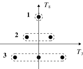
Figure 6: The figure shows the $\mathbf{\bar{6}}$ representation and its decomposition into $SU(2)$ subgroups: this is $\mathbf{\bar{6}}=\mathbf{1}\oplus\mathbf{2}\oplus\mathbf{3}$ with charges $T_{8}=+2\sqrt{3}/3,+\sqrt{3}/6,-\sqrt{3}/3$, respectively.

Then, we obtain the following four massless chiral fermions confined to the first brane: the right-handed $SU(2)$-singlet $\psi_{R}^{\mathbf{1}}$ with charge $Q=(0,+2/\sqrt{3})$; the two left-handed components of the $SU(2)$-doublet $\psi_{L}^{\mathbf{2}}$ with charges $Q=(-1/2,+1/2\sqrt{3})$ and $Q=(+1/2,+1/2\sqrt{3})$; and only one right-handed component from the triplet $\psi_{L}^{\mathbf{3}}$, with charge $Q=(0,-1/\sqrt{3})$. Figure 7 shows those components of the $\mathbf{\bar{6}}$ that confine to $z=0$.

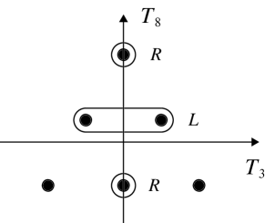
Figure 7: The figure shows those states of the $\mathbf{\bar{6}}$ that end up localized to $z=0$. The labels $L$ and $R$ indicate the chirality of the confined states.

When the effective Lagrangian is computed we find the appropriate quantum numbers for this sector to be identified with the quarks of the standard model. A significant difference with the lepton case, however, is the absence of interactions between quarks and the vector field $V_{\mu}^{i}$.

IV.4 Solving the hierarchy problem

We have seen that the electron and $W$-boson masses are $m_{e}=\sqrt{3/2}\phi_{0}\lambda_{\phi}$ and $M_{W}=\phi_{0}\lambda_{H}/2$ respectively. What is more, the quark masses are found to be proportional to $\phi_{0}\lambda_{\phi}$, of the same order as the electron mass. This is just the hierarchy problem for the particular case of the present model (recall that the $\lambda$-couplings are all of the same order).

A simple way to correct this problem is to introduce a new term in the definition of $Y$. For example, we could consider a new coupling $Y^{\prime}$ of the form:

$$Y^{\prime}=Y-y\,q\,v\,\Theta,$$ (56)

where $q$ is a dimensionless coefficient that could depend on the representation on which $Y^{\prime}$ is acting (observe the similarity of the new term with the old one $-y\,p\,u\,\Phi$, in $Y$). Then, after the scalars have acquired the v.e.v. discussed before, the $Y^{\prime}$ coupling becomes:

$$Y^{\prime}(z)=Y(z)-q(yvu)T_{8}.$$ (57)

The second term of this expression resembles the 5-D mass term of Eq. (1). Therefore, the fermion wave functions will be split around the branes and an exponential factor [like the one of Eq. (18)] will appear suppressing the couplings of Eq. (54). This results in a hierarchy between the mass scales of quarks, leptons and electroweak gauge bosons.

Observe that in the definition of $Y$ we could also include terms proportional to $\Phi^{2}$ and $\Theta^{2}$ with coefficients depending on the representation. They would provide additional terms contributing to the split of fermions around the brane.

IV.5 About the other branes

To finish, let us briefly mention that other branes are also formed in the bulk. They appear from the localization of the rest of the states in the $\mathbf{10}$ and $\mathbf{\bar{6}}$ representations. The most interesting brane is the “mirror brane” at $z=L/2$, which contains a copy of the electroweak model obtained at the first brane $z=0$ but with states having opposite chiralities. The rest of the branes (also determined by the condition $Y=0$) all contain different versions of $U(1)$ abelian gauge theories. Figure 8 shows the 5-D configuration obtained in the construction.

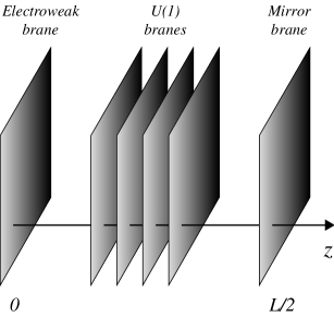
Figure 8: The figure sketches the disposition of branes in the 5-D bulk. The electroweak brane is located at $z=0$, while the mirror brane (a copy of the first brane but containing matter with opposite chirality) is located at $z=L/2$.

V Conclusions

In this paper we have obtained a simple realization of the electroweak model confined to a brane. The mechanism consisted in breaking the $SU(3)$ gauge symmetry down in $SU(2)\times U(1)$ through the localization of bulk fermions to the brane. The localization was produced by the coupling $Y$, of Eq. (48), between $SU(3)$ fermions and scalar fields with non-zero vacuum expectation values. As in the split fermion scenario, the four-dimensional fermions at the brane were found to be chiral. This allowed us to achieve the electroweak chiral structure by localizing those states (within given $SU(3)$-representations) with appropriate charges to the same brane. For example, the lepton sector was obtained from the $\mathbf{10}$ representation, while the quark sector was obtained from the $\mathbf{\bar{6}}$.

Remarkably, in this model it was possible to identify the Higgs field with the fifth component of the $SU(3)$ bulk gauge field (see gh1 ; gh2 ; gh3 ; gh4 ; gh5 ; gh6 for similar approaches). One problem with this result, however, is the apparent difficulty in generating the appropriate potential for the Higgs. Whether it is possible to obtain such a potential in this particular setup remains an open question.

Another feature of the present construction is the presence of two new fields coupled to the lepton sector of the standard model: A four-component vector field $V_{\mu}^{i}$ (that transforms like the Higgs under $SU(2)\times U(1)$ symmetry transformations) and a left-handed neutrino $N$ (with zero-hypercharge). The existence of these particles opens up interesting phenomenological possibilities. For instance, the nonobservation of $V$-bosons pair-production at LEP exp-W is an indication of the constraint:

$$M_{V}>104\mathrm{GeV}.$$ (58)

Nevertheless, from the results of this paper we should not expect a value $M_{V}$ significantly higher than $M_{Z}$ and $M_{W}$. At the same time, the mechanism generating the hierarchy between leptons, quarks and gauge bosons, is also suppressing the couplings between $V$ and leptons. If this is the case, then we could expect new phenomena associated with extra-dimensions in lepton-collider experiments in the near future.

Let us finish by mentioning that an important question that still needs to be addressed within this model is how to include the mixing between different families of leptons and quarks. For instance, in the case of leptons, the new neutrino $N$ could be playing some relevant role in the mixing of neutrinos.

References

- (1) I. Antoniadis, Phys. Lett. B 246, 377 (1990).
- (2) I. Antoniadis, C. Munoz and M. Quiros, Nucl. Phys. B 397, 515 (1993).
- (3) I. Antoniadis and K. Benakli, Phys. Lett. B 326, 69 (1994).
- (4) J.D. Lykken, Phys. Rev. D 54, R3693 (1996).
- (5) N. Arkani-Hamed, S. Dimopoulos and G. Dvali, Phys.Lett. B 429, 263 (1998).
- (6) I. Antoniadis, N. Arkani-Hamed, S. Dimopoulos, G. Dvali, Phys.Lett. B 436, 257 (1998).
- (7) V. A. Rubakov, Phys. Usp. 44, 871 (2001).
- (8) Csaba Csáki, TASI Lectures on Extra Dimensions and Branes, hep-ph/0404096.
- (9) V. A. Rubakov and M. E. Shaposhnikov, Phys. Lett. B 125, 136 (1983).
- (10) N. Arkani-Hamed and M. Schmaltz, Phys. Rev. D 61, 033005 (2000).
- (11) N. Arkani-Hamed, Y. Grossman and M. Schmaltz, Phys. Rev. D 61, 115004 (2000).
- (12) E. A. Mirabelli and M. Schmaltz, Phys. Rev. D 61, 113011 (2000).
- (13) G. Dvali, G. Gabadadze and M. Shifman, Phys. Lett. B 497, 271 (2001).
- (14) G. Dvali, M. Shifman, Phys. Lett. B 396, 64 (1997).
- (15) S. L. Dubovsky, V. A. Rubakov and P. G. Tinyakov, J. High Energy Phys. 08 (2000) 041.
- (16) I. Antoniadis, K. Benakli and M. Quiros, New J. Phys. 3, 20 (2001).
- (17) L. Hall, Y. Nomura and D. Smith, Nucl. Phys. B 639, 307 (2002).
- (18) G. Dvali, S. Randjbar-Daemi and R. Tabbash, Phys. Rev. D 65, 064021 (2002).
- (19) C. Csaki, C. Grojean and H. Murayama, Phys.Rev. D 67, 085012 (2003).
- (20) Gustavo Burdam and Yasunori Nomura, Nucl. Phys. B 656, 3 (2003).
- (21) C.A. Scrucca, M. Serone and L. Silvestrini, B 669, 128 (2003).
- (22) G. Abbiendi, et al. (The OPAL Collaboration), Eur. Phys. J. C 26, 321 (2003).