UNH-05-03, UCB-PTH-05/16
UPR-1119-T, NSF-KITP-05-29
hep-th/0505167

Supergravity Microstates for BPS Black Holes and Black Rings

Per Berglund^,a, Eric G. Gimon^,b,c and Thomas S. Levi^,d,e

^a Department of Physics, University of New Hampshire, Durham, NH 03824, USA.

^b Department of Physics, University of California, Berkeley, CA 94720, USA.

^c Theoretical Physics Group, LBNL, Berkeley, CA 94720, USA.

^d David Rittenhouse Laboratories, University of Pennsylvania, Philadelphia, PA 19104, USA.

^e Kavli Institute for Theoretical Physics, University of California, Santa Barbara, CA, 93106, USA.

We demonstrate a solution generating technique, modulo some constraints, for a large class of smooth supergravity solutions with the same asymptotic charges as a five dimensional 3-charge BPS black hole or black ring, dual to a $D1/D5/P$ system. These solutions are characterized by a harmonic function with both positive and negative poles, which induces a geometric transition whereby singular sources have disappeared and all of the net charge at infinity is sourced by fluxes through two-cycles joining the poles of the harmonic function.

1 Introduction and Summary

The black hole information puzzle [1] is a particularly striking example of the problems encountered when trying to combine quantum mechanics and gravity. Various computations in string theory have suggested that the usual picture of a black hole with an event horizon, then empty space with a central singularity, could be an emergent phenomena arising when we coarse grain over a set of microstates. A similar conjecture applies for the new black ring solutions [2, 3, 4, 5, 6, 7, 8]. Recently, Mathur and Lunin have made a stronger conjecture [9] (see [10] for a recent review) which holds that black hole microstates are characterized by string theory backgrounds with no horizons.

Up to now the main evidence for this conjecture involves finding microstates for two charge proto-black holes with no classical horizon area. Recently, Mathur et al [11, 12, 13] uncovered some three charge supergravity solutions with no horizon (see also [14]). Since these solutions exactly saturate a bound on angular momentum, they have the same asymptotic charges as a black hole whose horizon area classically vanishes. In [15] some finite temperature (non-supersymmetric) generalizations appear for these which correspond to black holes with finite size horizons; we are interested in finding microstates for BPS black holes which have already have finite size horizons for zero temperature.

Bena and Warner [16] (see also [17]) have developed a formalism for finding five dimensional supersymmetric solutions with three asymptotic charges and two angular momenta as reductions from M-theory. We will show how a general class of these solutions can be layed out which corresponds (modulo some consistency conditions) to $U(1)$ invariant microstates with the asymptotics of black objects with finite areas, dual to the $D1/D5/P$ system. We develop the simplest cases; some too simple, in fact, to look like black objects with non-vanishing horizons. The framework we lay out, however, exhibits strong potential for finding $U(1)$-invariant supergravity microstates for all five-dimensional black objects.

The Bena-Warner ansatz involves a fibration of the time coordinate over a hyperkahler base space. The key insight from [13] is that even if this base space is singular, a time fibration can be formulated such that the total space is completely smooth. This gives us access to a whole new class of base spaces: new two-cycles replace the origin of ${\bf R}^{4}$.

We will review the Bena-Warner ansatz in section 2 and then in section 3 we will offer a general form for a solution to these equations (a similar set of ansatz appears in [18, 19, 20, 21, 6, 22]) which are obviously smooth everywhere except at some orbifold points and possibly where the base space is singular. In section 4 we will demonstrate that our solution is smooth everywhere with no closed timelike curves or event horizons given three general sets of constraints. In section 5 we outline a simple class of examples for our formalism related to the solutions in [11, 12, 13]. They saturate a bound on rotation, and so correspond to microstates of black holes with no classical horizon. In section 6 we discuss how these examples can be generalized so as to include microstates for black holes which have finite size horizons. Finally we will briefly discuss further generalizations and future directions.

Work concurrent with this paper is also appearing in [23].

2 The Bena-Warner Ansatz and System of Equations

In [16] Bena and Warner neatly lay out an ansatz for a 1/8 BPS solution with three charges in five dimensions as a reduction from M-theory where the charges come from wrapping membranes on three separate $T^{2}$’s used to reduce from eleven dimensions. The five dimensional space is written as time fibered over a hyperkahler base space, $H\!K$. The resulting M-theory metric takes the form:

$$ds^{2}_{11}=-(Z_{1}Z_{2}Z_{3})^{-2/3}(dt+k)^{2}+(Z_{1}Z_{2}Z_{3})^{1/3}ds^{2}_{HK}+ds^{2}_{T^{6}},$$ (2.1)

where

$$ds^{2}_{T^{6}} = (Z_{1}Z_{2}Z_{3})^{1/3}\left(Z_{1}^{-1}(dz_{1}^{2}+dz_{2}^{2})+Z_{2}^{-1}(dz_{3}^{2}+dz_{4}^{2})+Z_{3}^{-1}(dz_{5}^{2}+dz_{6}^{2})\right).$$ (2.2)

The $Z_{i}$’s and $k$ are functions and one-form respectively on the hyperkahler base space, the three $T^{2}$’s have volumes $V_{i}$. The gauge field takes the form:

$$C_{(3)} = -(dt+k)\left(Z_{1}^{-1}\,dz_{1}\wedge dz_{2}+Z_{2}^{-1}\,dz_{3}\wedge dz_{4}+Z_{3}^{-1}\,dz_{5}\wedge dz_{6}\right)$$ (2.3)

$$+2\,a_{1}\wedge dz_{1}\wedge dz_{2}+2\,a_{2}\wedge dz_{3}\wedge dz_{4}+2\,a_{3}\wedge dz_{5}\wedge dz_{6},$$

where the $a_{i}$ are one-forms on the base space. After reduction on $T^{6}$ the C-field effectively defines three separate $U(1)$ bundles, with connections ${\cal A}_{i}=-(dt+k)Z^{-1}_{i}+2\,a_{i}$, on the 5-dimensional total space. If we now define the two-forms,

$$G_{i}=da_{i},$$ (2.4)

[16] show that the equations of motion reduce to the three conditions (here the Hodge operator refers only to the base space $H\!K$):

$$G_{i} = \star G_{i},$$ (2.5)

$$d\!\star\!dZ_{i} = 2s^{ijk}\,G_{j}\wedge G_{k},$$ (2.6)

$$dk+\star dk = 2\,G_{i}Z_{i}.$$ (2.7)

where we define the symmetric tensor $s^{ijk}=|\epsilon^{ijk}|$.

3 Solving the Equations and Asymptotics

In this section, we will first solve the Bena-Warner ansatz by selecting a base space $H\!K$ which has the property that the reduced five dimensional space is asymptotically flat. Written in Gibbons-Hawking form, the metric for this base space is:

$$ds^{2}_{HK}=H^{-1}\sigma^{2}+H(dr^{2}+r^{2}d\theta^{2}+r^{2}\sin^{2}\theta d\phi^{2}),$$ (3.1)

where $H$ is a positive function on ${\bf R}^{3}$ with integer poles and $\sigma$ is a one form on ${\bf R}^{3}$ of the form $d\tau+f_{a}dx^{a}$ ($\tau$ has period $4\pi$) satisfying

$$\star_{3}d\sigma=dH.$$ (3.2)

Asymptotic flatness with no $ADE$ identification basically forces the choice $H=1/r$ on us, this is fairly limiting. Following [13], however, we know that the time fibration can allow us to relax the hyperkahler condition on $H\!K$. We allow a singular pseudo-hyperkahler $H\!K$ (see [13] for a definition) so long as the total space with the time-fiber is smooth.

Our complete solution will be encoded using a set of 8 harmonic function on ${\bf R}^{3}$: $H,h_{i},M_{i}$ and $K$, generalizing the appendix in [13] patterned on [24]. These can take a fairly generic form, with constraints and relations that we will gradually lay out and then summarize.

3.1 The function $H$

Relaxing the hyperkahler conditions provides us with more general candidates for $H$, such as:

$$H=\sum_{p\,=1}^{N}\frac{n_{p}}{r_{p}},\qquad r_{p}=|\vec{r}_{p}|=|\vec{x}-\vec{x}_{p}|,\qquad\sum_{p\,=1}^{N}n_{p}=1.$$ (3.3)

The last sum guarantees that asymptotically we have an ${\bf R}^{4}$. Relaxing the condition that the $n_{p}$ be positive has allowed us to introduce an arbitrary number of poles, $N$, at positions $\vec{x}_{p}$. We can use this potential to divide ${\bf R}_{3}$ into a part where $H>0$ (Region I) and a compact (but not necessarily connected) part where $H<0$ (Region II). The two are separated by a domain wall where $H=0$ (from now we will refer to this as “the domain wall”). The metric in eq.(3.1) is singular at this domain wall, but we will see in the next section how the $t$-fibration saves the day. It does not, however, change the fact that with our choice of $H$ there are two-cycles, $S^{pq}$, coming from the fiber $\sigma$ over each interval from $\vec{x_{p}}$ to $\vec{x_{q}}$; it just makes them non-singular.

For convenience we define the following quantities:

$$\Pi^{r}=\prod_{p\,=1}^{N}r_{p},\;\;\Pi^{r}_{p}=\prod_{q\neq p}r_{q},\;\;\Pi^{r}_{ps}=\prod_{s\neq q\neq p}\!\!r_{q},\qquad f=\sum_{p\,=1}^{N}n_{p}\Pi^{r}_{p}.$$ (3.4)

Hence, $H$ can be written as $f/\Pi^{r}$. Note also that eq.(3.3) implies that $f\to r^{N-1}$ at asymptotic infinity, regardless of our choice of origin.

3.2 The Dipole Fields

To generate the $G_{i}$, it is useful to define harmonic functions on $H\!K$ that, up to a gauge transformation, fall off faster than $1/r$ as $r\to\infty$. To limit the scope of our discussion, we choose these to have poles in the same place as $H$.

$$h_{i}=\sum_{p\,=1}^{N}\frac{d_{i}^{(p)}}{4{r}_{p}}\,,\quad\sum_{p\,=1}^{N}d_{i}^{(p)}=0.$$ (3.5)

With these functions we define self-dual $G_{i}$’s:

$$G_{i}=d(h_{i}/H)\wedge\sigma-H\!\star_{3}d(h_{i}/H),$$ (3.6)

which have the requisite fall-off ($\star_{3}$ is the Hodge operator on ${\bf R}^{3}$). Note that we can always satisfy the condition in eq.(3.5) by applying the gauge transformation

$$h_{i}\to h_{i}-{1\over 4}\sum_{p}d^{(p)}_{i}\,H.$$ (3.7)

We can integrate the two-forms partially to get an expression for the $a_{i}$’s:

$$a_{i}=(h_{i}/H)\,\sigma+a_{ia}dx^{a},\qquad d(a_{ia}dx^{a})=-\star_{3}dh_{i}$$ (3.8)

where the $dx^{a}$ denote any complete set of one-forms on flat ${\bf R}^{3}$. Since we have chosen to localize the poles of the $h_{i}$ on top of the poles of $H$, these one-forms have no singularities except at $H=0$. It useful to define the dipole moments:

$$\vec{D}_{i}=\sum_{p\,=1}^{N}d^{(p)}_{i}\vec{x}_{p},$$ (3.9)

which control the asymptotics of our solution. Note that a priori these need not be parallel vectors such as in the asymptotics of a single black ring. Also, since $\sum_{p}d_{i}^{(p)}=0$, these dipole moments are independent of the choice of origin for ${\bf R}^{3}$. It is also useful to define, more locally, the relative dipole moments and to rewrite expressions as a function of these quantities:

$$d_{i}^{pq}=n_{p}d_{i}^{(q)}-n_{q}d_{i}^{(p)}\;\;\;\Rightarrow\qquad d_{i}^{(p)}=-\sum_{q=1}^{N}d_{i}^{pq},\qquad\vec{D}_{i}=-{1\over 2}\sum_{pq}d_{i}^{pq}\,(\vec{x}_{p}-\vec{x}_{q}).$$ (3.10)

The $d_{i}^{pq}$’s will appear almost everywhere in our solution. As we will see, they measure the various $U(1)$ fluxes through the two-cycle, $S^{pq}$, connecting $\vec{x}_{p}$ and $\vec{x}_{q}$.

3.3 The Monopole fields

The membrane charge at infinity can be read off from the C-field components with a time component. Looking at eq.(2.3) this means that the $Z_{i}$’s encode the three membrane charges $Q_{i}$, therefore they must have a falloff like

$$Z_{i}\to 1+{Q_{i}\over 4r}\qquad\textrm{as}\qquad r\to\infty.$$ (3.11)

since the asymptotic ${\bf R}^{4}$ radial coordinate is $R=2r^{1\over 2}$. Taking advantage of the natural radial distances in $H$ we can write arbitrary new harmonic functions,

$$M_{i}=1+\sum_{p\,=1}^{N}{Q^{(p)}_{i}\over 4r_{p}},\qquad\sum_{p\,=1}^{N}Q_{i}^{(p)}=Q_{i},$$ (3.12)

which have exactly the asymptotics above. We use these to write down the following ansatz for the $Z_{i}$’s

$$Z_{i} = M_{i}+2\,H^{-1}s^{ijk}h_{j}\,h_{k}.$$ (3.13)

The correction terms fall off like $1/r^{2}$ so they don’t mess up the asymptotics. They are necessary to satisfy the second equation of motion, eq.(2.6):

$$d\!\star\!dZ_{1}=4\,G_{2}\wedge G_{3},\qquad d\!\star\!dZ_{2}=4\,G_{1}\wedge G_{3},\qquad d\!\star\!dZ_{3}=4\,G_{1}\wedge G_{2},$$ (3.14)

up to some extra delta function sources. For the purposes of this paper, we will focus our attention on $Z_{i}$’s tuned so that they have no singularities apart from those at $H=0$. This removes the delta function sources in eq.(3.14) and allows us to write the $Q_{i}^{(p)}$ explicitly as:

$$Q_{i}^{(p)}=-{s^{ijk}\over 2n_{p}}\,{d_{j}^{(p)}\,d_{k}^{(p)}}.$$ (3.15)

We can now rewrite the $Z_{i}$ in the following form:

$$Z_{i}=1-{s^{ijk}\over 4f}\sum_{p,q}\frac{d_{j}^{pq}d_{k}^{pq}\Pi^{r}_{pq}}{4n_{p}n_{q}},$$ (3.16)

where we have used the quantities $f$ and $\Pi^{r}_{p}$ from eq.(3.4). This implies an alternate form for the $Q_{i}$,

$$Q_{i}=\sum_{p,q}Q_{i}^{pq},\qquad{\rm where}\qquad Q_{i}^{pq}=-\frac{s^{ijk}d_{j}^{pq}d_{k}^{pq}}{4n_{p}n_{q}},$$ (3.17)

which makes clear that we can also think of the total charge at infinity as coming from a sum of contributions from each two-cycle $S^{pq}$.

3.4 The Angular Momentum

Finally, lets look at the angular momentum. We use the natural basis

$$k=k_{0}\,\sigma+k_{a}\,dx^{a},$$ (3.18)

with the $d\alpha^{i}$ a complete basis of one-forms on ${\bf R}^{3}$. Our ansatz is now:

$$k_{0} = K+8H^{-2}\,h_{1}\,h_{2}\,h_{3}+H^{-1}\,M_{1}\,h_{1}+H^{-1}\,M_{2}\,h_{2}+H^{-1}\,M_{3}\,h_{3}$$

$$= K-4H^{-2}\,h_{1}\,h_{2}\,h_{3}+Z_{i}\,(h_{i}/H)=\bar{K}+Z_{i}\,(h_{i}/H)$$

$$\star_{3}d(k_{a}dx^{a}) = HdK-K\,dH+h_{i}\,dM_{i}-M_{i}\,dh_{i}$$

$$= H\,d\bar{K}-\bar{K}\,dH+h_{i}\,dZ_{i}-Z_{i}\,dh_{i}$$

Here we have defined a new harmonic function, $K$, and its partner function, $\bar{K}$:

$$K=\sum_{p\,=1}^{N}\left({\ell_{p}\over r_{p}}\right),\qquad\bar{K}=K-4H^{-2}\,h_{1}\,h_{2}\,h_{3}.$$ (3.21)

The regularity of $k$ is important here. There is an integrability condition on eq. (3.4) which basically requires that “$d\star_{3}$” of that equation is zero; this is trivially satisfied everywhere except at the poles of our harmonic functions. We would like the one-form $k$ to have no singularities except at $H=0$ and for $k_{a}dx^{a}$ to be a globally well defined one-form everywhere on ${\bf R}^{3}$ with an asymptotic fall-off like $1/r$. This turns out to be possible if we use the freedom to add any closed form of our choice to $k_{a}dx^{a}$, and demand:

$$\ell_{p}=\frac{d^{(p)}_{1}d^{(p)}_{2}d^{(p)}_{3}}{16n_{p}^{2}},\qquad k_{0}|_{r_{p}=0}=0.$$ (3.22)

The first condition removes poles in $\bar{K}$, the second condition insures that $d^{2}(k_{a}dx^{a}=0)$ everywhere, i.e. that $k_{a}dx^{a}$ is globally well defined. With the first condition we can rationalize our form for $k_{0}$ a little bit:

$$k_{0} = \sum_{p\,=1}^{N}\sum_{i}\frac{d_{i}^{(p)}\Pi^{r}_{p}}{4f}+{1\over 16\Pi^{r}f^{2}}\Bigg{[}\sum_{p,q,s}\Big{(}d_{1}^{(p)}d_{2}^{(p)}d_{3}^{(p)}\frac{n_{q}n_{s}}{n_{p}^{2}}-d_{1}^{(p)}d_{2}^{(q)}d_{3}^{(s)}\Big{)}\Pi^{r}_{p}\Pi^{r}_{q}\Pi^{r}_{s}$$

$$-s^{ijk}\sum_{p\,=1}^{N}d_{i}^{(p)}\Pi^{r}\Pi^{r}_{p}\sum_{q,s}\frac{d_{j}^{qs}d_{k}^{qs}\Pi^{r}_{qs}}{4n_{q}n_{s}}\Bigg{]}$$

This allows us to solve for $k_{0}=0$ at the points ${r}_{p}=0$, boiling down to

$$0=\sum_{i}d^{(p)}_{i}\;+\sum_{q}{1\over 4n_{p}^{2}n_{q}^{2}}{1\over r_{pq}}\prod_{i}d_{i}^{pq}$$ (3.24)

where $r_{pq}=|\vec{x}_{p}-\vec{x}_{q}|$. This puts at most $N-1$ independent constraints on the relative positions of the poles. Of course, all the $r_{pq}$ have to be non-negative, therefore a bad choice of $d_{i}^{pq}$ may lead to no solution at all! Note, also, that if any of the $d_{i}^{pq}$ vanishes, then the corresponding $r_{pq}$ will not appear in these constraints.

Using eqs.(3.22) and (3.24), we can rewrite eq.(3.4) as:

$$\star_{3}d(k_{a}dx^{a})=-\sum_{p,q}{1\over 32n_{p}^{2}n_{q}^{2}}\prod_{i}{d_{i}^{pq}\over r_{pq}r_{q}^{2}r_{p}^{2}}\Big{(}(r_{pq}-r_{p})r_{p}dr_{q}-(r_{pq}-r_{q})r_{q}dr_{p}\Big{)}$$ (3.25)

If we define $\phi_{pq}$ as the right-handed angle about the directed line from $\vec{x_{p}}$ to $\vec{x_{q}}$, we can integrate the expression above explicitly to get:

$$k_{a}dx^{a}=\sum_{p,q}{1\over 64n_{p}^{2}n_{q}^{2}}\prod_{i}{d_{i}^{pq}\over r_{pq}^{2}r_{q}r_{p}}(r_{p}+r_{q}-r_{pq})\Big{(}r_{pq}^{2}-(r_{p}-r_{q})^{2}\Big{)}\,d\phi_{pq}.$$ (3.26)

The two-form $dk$ naturally splits into a self-dual and anti-self-dual part. The split gives:

$$dk_{L}=(dk+\star\,dk)/2 = \,Z_{i}G_{i}$$ (3.27)

$$dk_{R}=(dk-\star\,dk)/2 = (d\bar{K}\wedge\sigma+H\!\star_{3}\!d\bar{K})+(h_{i}/H)\,(dZ_{i}\wedge\sigma+H\!\star_{3}\!dZ_{i})$$ (3.28)

Notice that we have correctly solved eq.(2.7) and also that $K$ contributes only to the anti-self-dual part of $dk$. Looking at the asymptotics, these tensors look like:

$$dk_{L} \to \sum_{i}G_{i}\to{1\over 4}\left[d\left({\sum_{i}4\vec{D}_{i}\cdot\hat{r}\over 4r}\right)\wedge\sigma-{1\over 4r}\!\star_{3}\!d\left({\sum_{i}4\vec{D}_{i}\cdot\hat{r}\over r}\right)\right]$$ (3.29)

$$dk_{R} \to {\sum_{p=1}^{N}16\ell_{p}}\,\cdot\,{1\over 4}\Big{[}d\left({1\over 4r}\right)\wedge\sigma+{d\sigma\over 4r}\Big{]}$$

From these expressions we can read the magnitudes of the angular momenta as measured at infinity. They take the values :

$$J_{L} = {4G_{5}\over\pi}j_{L}=|4\sum_{i}\vec{D}_{i}|,$$ (3.30)

$$J_{R} = {4G_{5}\over\pi}j_{R}=16\,\sum_{p=1}^{N}\ell_{p},$$ (3.31)

The $j_{L,R}\in{\bf Z}$ and $G_{5}$ is the five-dimensional Newton’s constant, which has length dimensions three and takes the value $G_{5}=16\pi^{7}\ell_{P}^{9}\prod_{i}V_{i}^{-1}.$

4 Smoothness of the Solution

So far, we have proposed general forms for the $G_{i}$, $Z_{i}$ and $k$ which satisfy the equations (2.5-2.7). The next step is to demonstrate that we can exhibit solutions without any singularities. Since our base space $H\!K$ is singular when $H\to 0$ it seems natural to check that the full metric and the C-field are free of singularities near this domain wall. In this section, we will demonstrate how, with the most general harmonic functions, we avoid any singularities at the domain wall. We will also address other potential pitfalls which might render our solution unphysical.

Assuming that none of the poles in the $h_{i},M_{i}$ and $K$ overlap with the domain wall, we see that $a_{i},Z_{i}$ and $k$ have the following expansions as $H\to 0$:

$$a_{i} = (h_{i}|_{0}H^{-1})\,\sigma+{\cal O}(H^{0}),$$ (4.1)

$$Z_{i} = Z_{i,-1}H^{-1}+{\cal O}(H^{0})=2s^{ijk}h_{j}|_{0}h_{k}|_{0}\,H^{-1}+{\cal O}(H^{0}),$$

$$\sigma = \sigma_{0}+H\sigma_{1}+{\cal O}(H^{2}),$$

$$k = (k_{0,-2}H^{-2})\,\sigma+(k_{0,-1}\sigma)H^{-1}\,+k_{0,0}\,\sigma+k_{a}|_{0}dx^{a}+{\cal O}(H).$$

For notational simplicity in section 4.1 we will refer to all non-singular variables (such as $k_{a}$ or $h_{i}$) by there values at $H=0$ without including a subscript.

4.1 The C-field and Metric as $H\to 0$

A quick inspection of the C-field in eq.(2.3) near the domain wall shows that potential singularities appear only in the purely spatial part, and only at order $H^{-1}$. The dangerous terms are of the form

$$H^{-1}\left(2h_{i}-(Z_{i}^{-1}k_{0,-2}\right)\sigma_{0}\wedge\textrm{Vol}_{T^{2}_{i}}$$ (4.2)

This singular term goes like (with no sum on $i$):

$$2h_{i}H^{-1}-s^{ijk}H\left(2h_{j}h_{k}+{\cal O}(H)\right)^{-1}H^{-2}\left(4s^{ijk}h_{i}h_{j}h_{k}+{\cal O}(H)\right)=0\cdot H^{-1}+{\cal O}(H),$$ (4.3)

so it cancels out generically. The metric has singularities of leading order $H^{-2}$ and subleading order $H^{-1}$, coming from the part of the metric which contains $\sigma$

$$-(Z_{1}Z_{2}Z_{3})^{-2/3}\,k^{2}+(Z_{1}Z_{2}Z_{3})^{1/3}H^{-1}\sigma^{2}=(Z_{1}Z_{2}Z_{3})^{-2/3}\left(-k^{2}+(Z_{1}Z_{2}Z_{3})H^{-1}\sigma^{2}\right)$$ (4.4)

Up to a finite coefficient, the singular piece is proportional to:

$$H^{-2}\left(-k_{0,-2}^{2}+(Z_{1}Z_{2}Z_{3})|_{-3}\right)(\sigma_{0}^{2}+2H\sigma_{1}\sigma_{0})+H^{-1}\left(-2k_{0,-2}k_{0,-1}+(Z_{1}Z_{2}Z_{3})|_{-2}\right)\sigma_{0}^{2}$$ (4.5)

We can see that these singular terms vanish for our ansatz, since:

$$-(k_{0,-2})^{2}+(Z_{1}Z_{2}Z_{3})|_{-3} = -64h_{1}^{2}h_{2}^{2}h_{3}^{2}+(4h_{2}h_{3})(4h_{1}h_{3})(4h_{1}h_{2})=0,$$ (4.6)

$$-2k_{0,-2}k_{0,-1}+(Z_{1}Z_{2}Z_{3})|_{-2} = -16h_{1}h_{2}h_{3}(M_{i}h_{i})+(M_{1}(4h_{1}h_{3})(4h_{1}h_{2})+\textrm{perms})=0.$$

4.2 Zeroes of the $Z_{i}$

Looking at eq.(2.3) or the determinant of the metric, $\sqrt{-g_{11}}=(Z_{1}Z_{2}Z_{3})^{1/3}\,H\,\sqrt{g_{{\bf R}^{3}}},$ we see that to avoid singularities it is necessary for $Z_{i}\neq 0$. We have a simple tactic for enforcing the non-vanishing of the $Z_{i}$: we demand that they obey

$$Z_{i}H>0\qquad\forall i\in{1,2,3}$$ (4.7)

everywhere. We choose a convention where the $Z_{i}$’s are negative at infinity, so this means that in Region I the $Z_{i}$ must remain positive, while in Region II this means that the $Z_{i}$ must remain negative. This uniformity also implies that $(Z_{1}Z_{2}Z_{3})^{1/3}$ is negative inside and positive outside, and guarantees that combinations like $(Z_{1}Z_{2}Z_{3})^{-2/3}$ and $Z_{i}^{-1}(Z_{1}Z_{2}Z_{3})^{1/3}$ remain positive everywhere. Using eq. (3.16), we see that the bound above can be written as:

$$4f-s^{ijk}\sum_{p,q}\frac{d^{pq}_{j}d_{k}^{pq}\Pi^{r}_{pq}}{4n_{p}n_{q}}>0\qquad\forall i\in{1,2,3}.$$ (4.8)

In section 5, we will show that with two poles, this bound is automatically satisfied modulo some relative sign conditions on the $d^{pq}_{i}$. However, in general eq.(4.8) will provide a non-trivial constraint on the relative positions of the $\vec{x_{p}}$; if solutions exist these conditions will define boundaries for the moduli space of solutions.

4.3 Closed timelike curves and horizons

Naively the $\sigma$ fibration has the potential to become timelike, thus creating closed timelike curves. To avoid this, we need to make sure the negative term proportional to $k^{2}$ doesn’t overwhelm the positive term from the base space. This means that we need to keep:

$$-(Z_{1}Z_{2}Z_{3})^{-2/3}\Big{(}k_{0}^{2}-Z_{1}Z_{2}Z_{3}H^{-1})\Big{)}\geq 0,$$ (4.9)

so that the norm of the vector in the $\sigma$ direction remains spacelike. Since the $Z_{i}$ have been tuned to avoid any poles except at $H=0$, and since the prefactor above is always positive, we only have to worry about the second term in the product. In general this is a complicated function, however, we can still exclude CTC’s along the $\sigma$ fiber in the neighborhood of the poles of $H$, $r_{p}=0$. There it is easy to see using eq.(3.24) that $k_{0}^{2}$ vanishes faster than $r_{p}$, insuring that loops along the $\sigma$ fiber will remain space-like.

We will exclude more general CTC’s in our five dimensional reduced space by requiring that this space be stably causal, i.e we will demand that there exists a smooth time function whose gradient is everywhere timelike [25]. Our candidate function is the coordinate $t$, and it qualifies as a time function if

$$-g^{\mu\nu}\partial_{\mu}t\partial_{\nu}t=-g^{tt}=\left(Z_{1}Z_{2}Z_{3}\right)^{-1/3}H^{-1}\left((Z_{1}Z_{2}Z_{3})H-H^{2}\,k_{0}^{2}-g^{ab}_{{\bf R}^{3}}k_{a}k_{b}\right)>0$$ (4.10)

We will leave for future work the question of possible extra constraints on the relative pole positions which come from this condition.

Granted the time function $t$, we can now proceed to show that there are no event horizons. The vector $\partial_{r}$ has a norm,

$$g_{rr}=(Z_{1}Z_{2}Z_{3})^{-2/3}\left((Z_{1}Z_{2}Z_{3})H-k_{r}^{2}\right)\geq-g^{tt},$$ (4.11)

which is positive everywhere due to eq.(4.10). Consider the following vector field:

$$\xi=\left({g_{rr}\over-g^{tt}}\right)^{1/2}g^{t\mu}\partial_{\mu}+\epsilon\,\partial_{r}.$$ (4.12)

The norm of $\xi$ is

$$\|\xi\|=-g_{rr}\left(1-\epsilon^{2}\right)$$ (4.13)

For $\epsilon<1$ this is always negative, therefore trajectories generated by this vector field will always be timelike. If we also choose $\epsilon>0$, these trajectories will always eventually reach asymptotic infinity and so there can be no event horizon.

4.4 Topology of the $\sigma$-fibration

The $\sigma$-fibration is preserved after the corrections in the full metric. Notice that the base metric has orbifold points with identification on the $\sigma$ fiber. The order of these points can be determined by the following calculation. For any given two-sphere on the base ${\bf R}^{3}$, we can determine the first Chern class, $c_{1}$, of the $\sigma$ fibration $U(1)$ bundle by integrating $d\sigma$ over that 2-sphere and then using Stoke’s theorem to turn that into an integral over the inside $B^{3}$:

$$\int_{S^{2}}d\sigma = \int_{S^{2}}\star_{3}dH=\int_{B^{3}}d\star_{3}dH=\sum_{p}\int_{B^{3}}n_{p}\,\delta^{3}(\vec{r}-\vec{r_{p}}).$$ (4.14)

This yields an integer which counts the poles inside of $S^{2}$. If this integer is zero, the topology of the $\sigma$-fiber over this $S^{2}$ is $S^{2}\times S^{1}$, if the integer is $\pm 1$ then the topology is that of $S^{3}$. Any larger integer $m$ will give the topology $S^{3}/Z_{m}$.

If we want to understand the corrections to the fibration from the whole metric, we rewrite the $\sigma$-fiber piece as:

$$(Z_{1}Z_{2}Z_{3})^{-2/3}(Z_{1}Z_{2}Z_{3}H^{-1}-k_{0}^{2})(\sigma-Ak_{a}dx^{a})^{2},\qquad A=\frac{Hk_{0}}{Z_{1}Z_{2}Z_{3}-Hk_{0}^{2}}.$$ (4.15)

For a given $S^{2}$, the correction to $c_{1}$ of the $\sigma$ bundle is

$$\int_{S^{2}}d(Ak_{a}dx^{a}) = \int_{S^{2}}(dA\wedge k_{a}dx^{a}+A\wedge d(k_{a}dx^{a}))$$

$$= \int_{B^{3}}(d^{2}A)\wedge k_{a}dx^{a}+A\wedge d\star_{3}(H\,d\bar{K}-\bar{K}\,dH+h_{i}\,dZ_{i}-Z_{i}\,dh_{i})=0.$$

The first of these terms is trivially zero, while the second vanishes due to eq. (3.22). Therefore, there are no corrections to the $\sigma$-fiber’s topology.

4.5 Topology of the Gauge Fields

Another interesting topological aspect for our solution is the topology of the C-field. We can gain a clearer picture of this by considering a membrane, labelled ${\cal M}_{i}$ wrapped on the torus $T_{i}$. This effectively yields a charged particle in the five-dimensional reduced space with charge,

$$e_{i}=V_{i}\,\tau_{2}=\frac{V_{i}}{(2\pi)^{2}\ell_{P}^{3}},$$ (4.17)

which experiences a gauge-field and field strength:

$${\cal A}_{i}=2a_{i}-Z_{i}^{-1}(dt+k),\qquad F_{i}=d{\cal A}_{i}.$$ (4.18)

For quantum consistency of the wave function for probe charges $e_{i}$, we usually require that on the five-dimensional space that the field strength be an integral cohomology class; the properly normalized integral of this class on a regular two-cycle should yield an integer. The compact two-cycles in our geometry, $S^{pq}$, are represented by line segments on ${\bf R}^{3}$ between two points $\vec{x}_{p}$ and $\vec{x}_{q}$ where the function $H$ blows up, along with the fiber $\sigma$. Of course, if either $n_{p}$ or $n_{q}$ is larger than one, the corresponding $S^{2}$ will have orbifold singularities. This means we should look for an integral cohomology class on the universal cover of $S^{pq}$, i.e. $n_{p}\cdot n_{q}$ times our original cycle.

The arguments above lead us to define an integer for each two-cycle, $S^{pq}$, derived from the following flux integral (all forms are pulled back to the two-cycle):

$$m^{(pq)}_{i}=n_{p}\,n_{q}\,{e_{i}\over 2\pi}\int_{\vec{x}_{p}}^{\vec{x}_{q}}\int_{\sigma}\,F_{i}d\tau ds=2n_{p}\,n_{q}\,e_{i}\;{\cal A}_{i}\Big{|}_{p}^{q}=2n_{p}\,n_{q}\,e_{i}\,(2a_{i}-Z_{i}^{-1}k_{0})\Big{|}_{p}^{q}$$ (4.19)

To evaluate this, we can use the fact that $k_{0}\to 0$ at the points where the $\sigma$ fiber degenerates. Thus,

$$m^{(pq)}_{i}=n_{p}\,n_{q}\,e_{i}\,\Big{(}{d^{\cdot}_{i}\over n_{p}}\Big{)}\Big{|}_{p}^{q}=e_{i}\Big{(}n_{p}\,d^{(q)}_{i}-n_{q}\,d^{(p)}_{i}\Big{)}=e_{i}d_{i}^{pq}.$$ (4.20)

Our story, however, does not end here. Near each orbifold point $p$, as mentioned above, the local geometry is a cone over $S^{3}/{\bf Z}_{n_{p}}$. This has $\pi_{1}=Z_{n_{p}}$ and implies that we have the possibility of a discrete Wilson line for each gauge field with a phase of the form $2\pi\,m^{(p)}_{i}/n_{p}$ where $m^{(p)}_{i}\in{\bf Z}$ (essentially we are using the fact that $H^{2}(S^{3}/{\bf Z}_{n_{p}})=Z_{n_{p}}$). The invariance of the local gauge field under a shift of $m_{i}^{(p)}$ by $n_{p}$ can be implemented by a gauge transformation similar to that of eq.(3.6). Looking at the gauge field ${\cal A}_{i}$ near one of the orbifold points, for example along the $\sigma$ fiber, we see that the Wilson line phase is:

$$2\pi\,\left(4e_{i}h_{i}/H\right)\Big{|}_{p}=2\pi\,m^{(p)}_{i}/n_{p}.$$ (4.21)

This implies a quantization for the $d_{i}^{(p)}$ of the form:

$$d^{(p)}_{i}=m^{(p)}_{i}/e_{i}=\frac{(2\pi)^{2}\ell_{P}^{3}}{V_{i}}\,m^{(p)}_{i},$$ (4.22)

with several consequences. First, the cohomology requirement in eq.(4.20) is trivially satisfied: $m_{i}^{(pp^{\prime})}=n_{p}m^{(p^{\prime})}_{i}-n_{p^{\prime}}m^{(p)}_{i}$. Second, unless all the $m^{(p)}_{i}$ at a given point $p$ are multiples of $n_{p}$ or on one of it’s divisors, the singularity is “frozen” or partially “frozen” . Finally, if we use our formula (3.15) for the monopole charges, we get:

$$Q^{(p)}_{i}=-{4G_{5}e_{i}\over\pi}\,s^{ijk}\frac{m^{(p)}_{j}m^{(p)}_{k}}{2n_{p}}.$$ (4.23)

and so the quantized membrane charge at infinity will be

$$N_{i}=\frac{\pi}{4e_{i}G_{5}}Q_{i}=\frac{\pi}{4e_{i}G_{5}}\sum_{p=1}^{N}Q^{(p)}_{i}=-\sum_{p=1}^{N}s^{ijk}\frac{m^{(p)}_{j}m^{(p)}_{k}}{2n_{p}}=-\sum_{p,q}s^{ijk}\frac{m^{pq}_{j}m^{pq}_{k}}{4n_{p}n_{q}}.$$ (4.24)

Note that the fact that the $N_{i}$’s are integers written as a sum of rational numbers add further constraints on the $m_{i}^{(p)}$’s or $m_{i}^{pq}$’s.

4.6 Summary of Conditions

We finish this section by summarizing the exact conditions which will define a smooth (modulo orbifold points) and regular 11-dimensional supergravity solution with three membrane charges and 4 supersymmetries, with no CTC’s or event horizons. The solution is completely parameterized by a set of poles on ${\bf R}^{3}$ with quantized residues $n_{p}$ and quantized fluxes $m^{pq}_{i}$. These, and the quantities that depend on them, must satisfy the following conditions:

$$1) \sum_{i}d^{(p)}_{i}\;+\sum_{q}{1\over 4n_{p}^{2}n_{q}^{2}}{1\over r_{pq}}\prod_{i}d_{i}^{pq}=0,$$ (4.25)

$$2) Z_{i}H>0\qquad\forall i\in{1,2,3},$$ (4.26)

$$3) (Z_{1}Z_{2}Z_{3})H-H^{2}\,k_{0}^{2}-g^{ab}_{{\bf R}^{3}}k_{a}k_{b}>0.$$ (4.27)

These need not be independent conditions, for example it may be possible that condition $(1)$ implies $(3)$ implies $(2)$.

There exists a canonical solution for eq.(4.25), as long as the $d_{i}^{pq}$ are such that the $r_{pq}$ come out non-negative, of the form:

$$r_{pq}={1\over 4n_{p}^{2}n_{q}^{2}}{\prod_{i}d_{i}^{pq}\over\sum_{i}d_{i}^{pq}}.$$ (4.28)

It is not yet clear what extra conditions on the $d_{i}^{pq}$, if any, are required for this canonical solution to satisfy the other two constraint equations.

5 The Basic 2-Pole Example

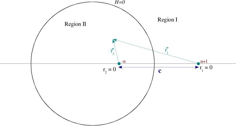
Figure 1: Basic 2-pole example has a spherical domain wall

Now that we have worked out a general formalism, let us illustrate it with the simplest example, the two pole solution; this reproduces the solutions of [11, 12, 13]. The simplest possible $H$ that interests us has two poles and can be written in the following form (w.l.o.g we choose $n>0$):

$$H=\frac{n+1}{r_{1}}+\frac{-n}{r_{2}}$$ (5.1)

where $r_{2}$ is defined as the distance in ${\bf R}^{3}$ from a point a distance $r_{12}=c$ below the origin on the $\phi$ symmetry axis; this gives $H\!K$ a $U(1)\times U(1)$ isometry. Note that with this choice of the function $H$, Region II is a spherical region with its center just below the point $r_{2}=0$ (see figure). The function $f$ is $f=-n\,r_{1}+(n+1)\,r_{2}$ and has as its minimum value $-n\,c$.

For the dipoles we choose $d_{i}^{(1)}=-d_{i}^{(2)}=d_{i}$. The $Z_{i}$’s and the net charges at infinity now take the simple form:

$$Z_{i}=1+{Q_{i}\over 4f},\qquad Q_{i}={s^{ijk}\over 2}\,\frac{d_{j}d_{k}}{n(n+1)}.$$ (5.2)

Notice that to guarantee positive $Q_{i}$’s, we must impose that the $d_{i}$’s all have the same sign. From eq.(3.22), we see that the poles of $K$ at $r_{1}=0$ and $r_{2}=0$ are:

$$\ell_{1}=\frac{d_{1}d_{2}d_{3}}{16(n+1)^{2}},\qquad\ell_{2}=-\frac{d_{1}d_{2}d_{3}}{16n^{2}}.$$ (5.3)

This gives a simple form to $k_{0}$:

$$k_{0}=\sum_{i}d_{i}\frac{r_{2}-r_{1}}{4f}-\frac{\Pi_{i}d_{i}}{n^{2}(n+1)^{2}}\frac{(n+1)r_{2}+nr_{1}}{16f^{2}}.$$ (5.4)

5.1 Solving the Constraints

In this simple case, there is a unique solution to the first constraints, eq.(4.25), which is the canonical solution:

$$c=\frac{1}{n^{2}(n+1)^{2}}\frac{\Pi_{i}d_{i}}{4\sum_{i}d_{i}}={1\over 4n(n+1)}\frac{Q_{1}Q_{2}Q_{3}}{(Q_{1}Q_{2}+Q_{2}Q_{3}+Q_{3}Q_{1})}.$$ (5.5)

Using this value and the fact that the minimum value for $f$ is $-n\,c$, the second constraint, eq.(4.26) can be easily checked. The final constraint, eq.(4.27), after some algebra, can be put in the form:

$$\Big{[}(M+4f)+D/(2r_{1}+2r_{2}+2c)\Big{]}/4r_{1}r_{2}>0$$ (5.6)

where $M=Q_{1}+Q_{2}+Q_{3}$ and $D=Q_{1}Q_{2}+Q_{2}Q_{3}+Q_{3}Q_{1}$. Each term in this product is manifestly positive, so we are guaranteed a smooth solution without CTC’s or event horizons.

5.2 Features of the Solution

The angular momenta can be read off from eq. (3.30):

$$J_{R} = -{d_{1}d_{2}d_{3}}\frac{2n+1}{n^{2}(n+1)^{2}}=\pm(2n+1)\sqrt{Q_{1}Q_{2}Q_{3}\over n(n+1)}$$ (5.7)

$$J_{L} = 4c\sum_{i}d_{i}=\pm 4c\sqrt{n(n+1)\over Q_{1}Q_{2}Q_{3}}(Q_{1}Q_{2}+Q_{2}Q_{3}+Q_{1}Q_{3})=\pm\sqrt{Q_{1}Q_{2}Q_{3}\over n(n+1)}.$$ (5.8)

The whole of the solution is completely determined by an integer $n$ and the three $d_{i}$’s or, more physically: $n$, the three charges $Q_{i}$ and a $\pm$ sign derived from a collective sign choice for $d_{i}$’s. We can extend this solution to negative $n$’s by taking $n\to-(n+1)$, which just flips the sign of $J_{R}$.

In general, if all three charges $Q_{i}$ are of order $Q$, large relative to $\ell_{P}^{2}$, then our system will be macroscopic for finite $n$, since $c\to Q/n(n+1)>>\ell_{P}^{2}$. If one of the charges is much smaller than the others, e.g. $Q_{3}<<Q_{1},Q_{2}$, then $c$ will be of order that smaller charge, and there will be high curvature regions if we don’t also have $Q_{3}>>\ell_{P}$.

To get a further understanding for the features of the two-pole solution, we draw the readers attention back to last part of eq.(5.2), which can be rewritten as

$$N_{i}={s^{ijk}\over 2}{m^{12}_{j}m^{12}_{k}\over n(n+1)}={s^{ijk}\over 2}{m_{j}m_{k}\over n(n+1)}.$$ (5.9)

Since the $N_{i}$ are integers, the product of any two integer $m_{j}$’s must be divisible by $n(n+1)$. Define $a=gcd\Big{(}m_{3},n(n+1)\Big{)}$ and it’s complement $b=n(n+1)/a$. The divisibility condition on the $m_{i}$’s implies that there exist integers $k_{i}$ and $k$ such that

$$m_{1}=b\,k_{1},\;m_{2}=b\,k_{2},\;m_{3}=a\,k_{3},\;\;\textrm{and}\;\;k_{1}\,k_{2}=a\,k.$$ (5.10)

These yield the following relations

$$N_{1}=k_{2}\,k_{3},\;N_{2}=k_{1}\,k_{3},\;N_{3}=b\,k,\;N_{1}N_{2}=(k\,k_{3})\,m_{3},$$ (5.11)

$$j_{L}={\pi\over 4G_{5}}J_{L}=(k\,k_{3}),\qquad j_{R}={\pi\over 4G_{5}}J_{R}=(2n+1)(k\,k_{3}).$$

Clearly the quantity $kk_{3}$, let us label it $N_{s}$, plays a prominent role.

If $k_{3}=1$ and $a$ divides $n$, there is a natural way of thinking about the numbers above. We take the third torus $T_{3}$ to have very small volume $V_{3}$. We then get a dual IIB description with $N_{1}$ and $N_{2}$ three-branes intersecting over a circle of radius $\ell_{P}^{3}/V_{3}$ with $N_{3}$ units of momentum going around the circle. They can intersect over one long string, wrapped $N_{1}N_{2}$ times around that circle or, more generally, $N_{s}=N_{1}N_{2}/m_{3}$ substrings wrapped $m_{3}$ times. If we start with no momentum, we have:

$$j_{L}=j_{R}=N_{s}=N_{1}N_{2}/m_{3}=kk_{3}$$ (5.12)

Following steps summarized in [12] we can apply a spectral flow shift of $2\tilde{n}$ to this CFT and get shifted values:

$$j_{R}\to j_{R}+2\tilde{n}\,N_{1}N_{2},\qquad N_{3}\to N_{s}\,\tilde{n}\,(\tilde{n}\,m_{3}+1)$$ (5.13)

Now define $n=\tilde{n}\,m_{3}$ and we get:

$$N_{3}=n(n+1)N_{s}/m_{3},\qquad j_{L}=N_{s},\qquad j_{R}=(2n+1)N_{s},$$ (5.14)

which fits nicely with eq. (5.11), except with the stronger assumption that $m_{3}$ divides $n$. Thus the states [12] are in a subclass of the generic two pole solution.

5.3 The Two Pole Solution as a Microstate

Since our original motivation was to find microstates for black holes and black rings, it is natural to ask if this geometry has the same asymptotics as one of those black objects.

Let us first consider the BMPV black hole [28]. Immediately, we run into a a problem: the basic solution above always has a non-zero $j_{L}$, so strictly speaking cannot be considered a microstate for the BMPV black hole in [28], which has $J_{L}=0$. For large values of $n$ and small values of $N_{s}$, however, it is possible to have $J_{R}$ be macroscopically large in Planck units, while $J_{L}$ remains of order the Planck length and can be coarse-grained away. In fact, the states that dominate the partition function for the CFT dual of the black hole (see [29] for a review) are in the single “long string” phase, which has $j_{L}=+1$. Taking this caveat into account, we see that in the large $n$ limit $J_{R}^{2}\to 4Q_{1}Q_{2}Q_{3}$, which means that our two -pole states are at best microstates of a zero area BMPV blackhole and as such cannot be considered as microstates for a proper BPS blackhole. We must look to other black objects.

By construction, the two-pole solution has $\vec{D}_{i}$’s which are parallel. This feature potentially qualifies it as a black ring microstate. Black rings, however, have more parameters than black holes, so we have to be careful in matching these. If we use the nomenclature in [5], we see that the parameters $q_{i}$ which appear in the expression for the horizon area only appear as $R^{2}q_{i}$ in the asymptotics, where $R$ is the inner radius of the ring. This leads to an ambiguity, since we match

$$4cd_{i}=R^{2}q_{i}.$$ (5.15)

As it turns out, $q_{i}$ and $d_{i}$ are quantized in the same units, so we have

$$R^{2}/4c=d_{i}/q_{i}=a/b,\qquad a,b\in{\bf Z}.$$ (5.16)

The black ring solutions require

$$\left(Q_{i}=\frac{s^{ijk}}{2}\frac{d_{j}d_{k}}{n(n+1)}\right)\geq\frac{s^{ijk}}{2}\,q_{j}q_{k}\;\;\Rightarrow\;\;\frac{a^{2}}{b^{2}}\geq n(n+1).$$ (5.17)

Without going into too much detail, if we compare our expressions for the angular momenta eq.(5.7) and eq.(5.8) with those in [5, 16], we find that the expressions for $J_{L}$ match (this match is independent of $N$) if we use eq.(5.15) but that our $J_{R}$ is always too small to qualify for a black ring. Only in the limit where we saturate the bound in eq.(5.17) and $n$ is very large do we start converging on the same value for $J_{R}$. At that point, our solution ends up sharing the asymptotics of a zero-area ring. This is a very similar story to that of the BMPV black hole.

In conclusion, the two-pole solution can at best appear as a microstate for “black” rings and “black” holes with zero horizon areas. In the context of the CFT microstates connection we developed earlier, this is none too surprising, as those states are unique given their charges and angular momenta. We also see that our supergravity solution does not appear to have any adjustable parameters, hence should not belong to the very numerous, i.e. entropic, class of states that should match a black object.

5.4 The Domain Wall

The surface $H=0$ has a radius:

$$R^{2}_{DW}=4r_{DW}=4c\,{Q_{1}Q_{2}Q_{3}\over J_{L}J_{R}}.$$ (5.18)

In the region near $r_{2}=0$ with radius of order $R=\sqrt{c}$, the functions $Z_{i}$ are locally constant and $k\propto r_{2}\,\sigma$, which means that the local metric is a $Z_{n}$ orbifold of a Gödel universe. This suggests that our solution is in fact the un-smeared version of the hypertube speculated about in [30] and is in fact a smooth resolution of the type of domain wall illustrated there.

Given that the hypertube-like solution we have found has completely smooth supergravity fields except for mild orbifold singularities, one is tempted to ask what physical features the surface at $H=0$ exhibits, if at all, to mark it’s presence. An associated issue is the question of just where the membrane charge detectable at infinity is sourced.

To answer the first question, it is interesting to consider a probe membrane in our background wrapping the $z_{1},z_{2}$ and $t$ directions. If we include a small velocity $v^{0}$ along the $\sigma$ fiber and $\vec{v}$ in the base space, we see that the probe action in the static gauge has an expansion which looks like:

$$e_{1}\int\Bigg{[}Z_{1}^{-1}\sqrt{(1+k_{0}v^{0}+k_{a}v^{a})^{2}-Z_{1}Z_{2}Z_{3}(H^{-1}v_{0}^{2}+Hg_{ab}v^{a}v^{b})}$$ (5.19)

$$-Z_{1}^{-1}(1+k_{0}v^{0}+k_{a}v^{a})+2a_{i0}v^{0}+2a_{ia}v^{a}\Bigg{]}d\lambda.$$

Clearly, there is no potential term, as can be expected for a BPS configuration. Away from the $H=0$ domain wall, we expand the action in small powers of the velocity, and we get:

$$e_{1}\int\Big{[}-{1\over 2}\,{Z_{2}Z_{3}}\left(H^{-1}v_{0}^{2}+Hg_{ab}v^{a}v^{b}\right)-2(a_{i0}v^{0}+a_{ia}v^{a})+{\cal O}(v^{3})\Big{]}d\lambda.$$ (5.20)

This is the action for a charged particle on $H\!K$ traveling in a magnetic field, albeit with variable mass. Near $H=0$, the mass parameter and magnetic field blow up! At this point, we can no longer work in the small $v$ approximation and must go back to the full action, itself always finite.

Another way to analyze the action as $H\to 0$, is to realize that $\partial_{t}$ becomes lightlike turning our static gauge into a light cone gauge. Expanding the worldline tangent for our wrapped membrane “particle” about the lightlike velocity vector $\partial_{t}$ gives us a theory with exact Galilean invariance. The momentum $p_{t}$ becomes the lightcone energy, and since the only mixed term in the line element looks like $dt\,\sigma$, $\tau$ seems to be the natural lightcone time variable. The interesting thing here is that $\tau$ is periodic, and $\partial_{\tau}$ is spacelike. Thus our membrane worldtheory takes on aspects of a finite temperature non-relativistic system! It is interesting to speculate about what this might mean for the process of “heating up” our solution to make it a microstate of a finite temperature near-BPS black hole, something like the states considered in [15]. We leave this for future work.

In summary, the domain wall at $H=0$ leads to some interesting behavior for the worldvolume on our probe brane, yet there is still no real discontinuity there and no vanishing of the probe kinetic term as for an enhancon [31], in fact just the opposite.

The charge in the hypertube has dissolved away, so where should we think of it existing? In our case, an alternate scenario to charges localized on a domain wall appears. We see instead a situation similar to that of the geometric transition in [32, 33], where a large number of D-branes wrapped on an $S^{3}$ at the tip of a cone over $S^{2}$ is replaced by flux on a non-contractible $S^{2}$ at the tip of a cone over $S^{3}$. We can take a decoupling limit for our solution by removing the $1$’s in the $Z_{i}$’s to get a five-dimensional space which is asymptotically an orbifold of $AdS_{2}\times S^{3}$. The infrared limit of the holographically dual theory should reflect the appearance of this geometric transition.

6 Adding More Poles

Clearly, if we want to achieve a more general solution which could have the same asymptotics as BPS black hole or black ring with a non-zero horizon area, the next step is to consider a solution with more poles, starting with three poles. We will see that this type of solution has more adjustable parameters, making it a more likely candidate.

6.1 Simple Three Pole Solutions

With three poles to play with, the simplest scenario is for $H$ to have two poles with residue $n_{1}=n_{2}=+1$ and one with residue $n_{3}=-1$. With these choices, the solution is completely smooth! We define the three radial distances from these poles as $r_{1},r_{2}$ and $r_{3}$, and corresponding dipoles $d^{(1)}_{i},d^{(2)}_{i}$ and $-(d^{(1)}_{i}+d^{(2)}_{i})$. One nice feature is that we can now vary the dipoles and $J_{L}$ by our choice of pole arrangements

We can further simplify our solution by working with dipoles that are diagonal in the three $U(1)$’s. This will guarantee that the dipole vector’s $\vec{D}_{i}$ will all be parallel, and thus allow comparison with BPS black rings, especially the ones in [4].

We start with probably the simplest example. $d_{i}^{(1)}=d_{i}^{(2)}=d$ and $d_{i}^{(3)}=-2d$. Then we find the set of equations eq. (4.25) become simply

$$r_{13}=r_{23}=\frac{d^{2}}{12},$$ (6.1)

with no restrictions on $r_{12}$. We must now satisfy $Z_{i}H>0$, eq. (4.26). This condition becomes

$$4(r_{2}r_{3}+r_{1}r_{3}-r_{1}r_{2})+d^{2}(r_{1}+r_{2})>0.$$ (6.2)

Using our values for $r_{13}$ and $r_{23}$ one can easily show this equation is satisfied at the three poles. It is also trivially satisfied at asymptotic infinity. Though it is difficult to show analytically, a numerical analysis confirms that it is satisfied everywhere for any value of $r_{12}$. Let us examine the implications of this. Without loss of generality we choose to place pole 3 at the origin, and pole 1 on the z-axis. Then, since there are no restrictions on $r_{12}$ we are free to place it anywhere on a circle of radius $r_{23}=r_{13}=d^{2}/12$. Let the angle 132 between segments ${13}$ and ${23}$  be called $\psi$. Then we find

$$\vec{D}_{i}=\frac{d^{3}}{12}[\hat{z}(1+\cos\psi)+\hat{x}\sin\psi].$$ (6.3)

One can read off the asymptotic charges for this solution. They are

$$Q_{1}=Q_{2}=Q_{3}=2d^{2},\ \ J_{R}^{2}=36d^{6},\ \ J_{L}^{2}=2d^{6}(1+\cos\psi).$$ (6.4)

One can easily see that while $Q_{i}$ and $J_{R}$ are independent of our pole arrangement, $J_{L}$ is very sensitive to it. We find that $0\leq J_{L}^{2}\leq 4d^{6}$, where the minimum value is reached when the negative pole (3) is in the middle of the two positive poles. The maximum value is reached when the two positive poles lie on top of each other, returning us to the 2-pole example from the previous section with $n=1$. Note also that even in this very simple three pole case, the last condition, eq. (4.27) is quite challenging; and we will not check it here.

For the purposes of finding microstates for black objects, adding a third pole already seems to help. For example, we can explicitly set $J_{L}$ to zero, which is characteristic of BMPV microstates. Unfortunately $J_{R}$ is still too large and saturates the BMPV bounds just as in the two-pole case. On the black ring side, things look more promising. As we adjust the angle $\psi$ the three dipoles have variable magnitude $2d\cos\psi/2\leq 2$, matching to a class of black rings with variable $J_{R}$, a function of the dipoles and smaller as we increase $\psi$. The upshot is that for $0<\psi<\pi$, we can now adjust the constant $a/b$ in eq.(5.16) so that the three-pole solution’s quantum number $j_{R}$ matches that of the black ring with the same dipoles and charges at infinity. Hence, modulo the CTC condition in eq.(4.27), we have identified supergravity microstates for black rings with finite-sized horizons.

6.2 Comments on the General Case

As we have seen, the three pole case allows us more freedom in positioning our poles. This freedom tends to only vary $J_{L}$ and the $\vec{D}_{i}$’s, hence it does not generate a large class of states with the same asymptotics. Ideally, we would like to be able to fix the $Q_{i}$’s, $\vec{D}_{i}$’s, $J_{L}$ and $J_{R}$ and still find many solutions. It seems reasonable to believe that adding more poles should allow us to have much larger moduli spaces of solutions, including substantial subspaces with the same $Q_{i}$’s,$D_{i}^{\prime}s$ and $J_{L,R}$; further work towards understanding BPS black ring and black hole microstates will requiring developing a better understanding of the general $n$-pole solution.

7 Discussion

The general picture that is emerging from our solution is that of generic five dimensional BPS three-charge black hole and black ring microstates coming from a harmonic function with a large number of poles. These solution are characterized by discrete choices, the $d_{i}^{pq}$’s, as well as continuous ones, the relative positions of the points $\vec{x_{p}}$. This dichotomy is reflected in the angular momenta, with $J_{R}$ clearly discrete in all cases while $J_{L}$ varies continuously requiring explicit quantization. Similarly, we see one set of exact constraints eq.(4.25) complemented by inequalities, inexact constraints, from eqs.(4.26-4.27).

It is likely that the dichotomy above arises from the explicit $U(1)$ invariance that permeates our solution, arising from our ansatz for the pseudo-hyperkahler base space in the Gibbons-Hawking form. This raises the question of what more general pseudo-hyperkahler base spaces look like. These general spaces could also have integer quantized fluxes on two-cycles, but these need no longer share the same $U(1)$ symmetry and so the asymptotic angular momenta would both vary continuously.

The exact $U(1)$ symmetry which we have, non-generic in five dimensions, can become an asset if we choose to use it to reduce to four dimensions. This can be done by simply adding a term of the form $1/R^{2}$ to the harmonic function, and relaxing the condition on the sum of the residues; most of our analysis will survive unchanged. This yields a substantial generalization of the four dimensional solutions in [21, 6, 22]. In those papers, solutions appear with a KK-monopole charge which is basically $\sum_{p}n_{p}$, but only allowing positive residues! Modulo constraints of the form in eqs.(4.25-4.27), the possibility of adding negative residues to the poles of $H$ greatly broadens this class of supersymmetric four dimensional solutions. If we make $\tau$ the M-direction, the appearance of negative poles corresponds to having anti-D6-branes while keeping the supersymmetries of D6-branes, this is similar to what happens in [34]. The appearance of both D-branes and anti-D-branes in a black hole microstate is something we have learned to expect in near-extremal systems to but is new to extremal ones.

We close by stressing what we feel is the most important idea emerging from our analysis: supergravity solutions dual to wrapped brane bound states replace a core region which naively would have a naked singularity or a horizon with a core region containing a “foam” of new topologically nontrivial cycles. This is a fascinating combination of Vafa etal.’s geometric transitions picture [32, 33] and melting crystal space-time foam picture [35, 36] which will certainly attract future attention.

References

- [1] S. W. Hawking, “Particle creation by black holes,” Commun. Math. Phys. 43 (1975) 199–220.
- [2] H. Elvang, “A charged rotating black ring,” Phys. Rev. D68 (2003) 124016, hep-th/0305247.
- [3] H. Elvang and R. Emparan, “Black rings, supertubes, and a stringy resolution of black hole non-uniqueness,” JHEP 11 (2003) 035, hep-th/0310008.
- [4] H. Elvang, R. Emparan, D. Mateos, and H. S. Reall, “A supersymmetric black ring,” Phys. Rev. Lett. 93 (2004) 211302, hep-th/0407065.
- [5] H. Elvang, R. Emparan, D. Mateos, and H. S. Reall, “Supersymmetric black rings and three-charge supertubes,” Phys. Rev. D71 (2005) 024033, hep-th/0408120.
- [6] H. Elvang, R. Emparan, D. Mateos, and H. S. Reall, “Supersymmetric 4D rotating black holes from 5D black rings,” hep-th/0504125.
- [7] R. Emparan and H. S. Reall, “A rotating black ring in five dimensions,” Phys. Rev. Lett. 88 (2002) 101101, hep-th/0110260.
- [8] R. Emparan, “Rotating circular strings, and infinite non-uniqueness of black rings,” JHEP 03 (2004) 064, hep-th/0402149.
- [9] O. Lunin and S. D. Mathur, “Metric of the multiply wound rotating string,” Nucl. Phys. B610 (2001) 49–76, hep-th/0105136.
- [10] S. D. Mathur, “The fuzzball proposal for black holes: An elementary review,” hep-th/0502050.
- [11] S. Giusto, S. D. Mathur, and A. Saxena, “Dual geometries for a set of 3-charge microstates,” Nucl. Phys. B701 (2004) 357–379, hep-th/0405017.
- [12] S. Giusto, S. D. Mathur, and A. Saxena, “3-charge geometries and their CFT duals,” Nucl. Phys. B710 (2005) 425–463, hep-th/0406103.
- [13] S. Giusto and S. D. Mathur, “Geometry of D1-D5-P bound states,” hep-th/0409067.
- [14] O. Lunin, “Adding momentum to D1-D5 system,” JHEP 0404, 054 (2004) [arXiv:hep-th/0404006].
- [15] V. Jejjala, O. Madden, S. F. Ross, and G. Titchener, “Non-supersymmetric smooth geometries and D1-D5-P bound states,” hep-th/0504181.
- [16] I. Bena and N. P. Warner, “One ring to rule them all … and in the darkness bind them?,” hep-th/0408106.
- [17] J. B. Gutowski and H. S. Reall, “General supersymmetric AdS(5) black holes,” JHEP 04 (2004) 048, hep-th/0401129.
- [18] F. Denef, “Supergravity flows and D-brane stability,” JHEP 08 (2000) 050, hep-th/0005049.
- [19] F. Denef, B. R. Greene, and M. Raugas, “Split attractor flows and the spectrum of BPS D-branes on the quintic,” JHEP 05 (2001) 012, hep-th/0101135.
- [20] B. Bates and F. Denef, “Exact solutions for supersymmetric stationary black hole composites,” hep-th/0304094.
- [21] D. Gaiotto, A. Strominger, and X. Yin, “5D black rings and 4D black holes,” hep-th/0504126.
- [22] I. Bena, P. Kraus, and N. P. Warner, “Black rings in Taub-NUT,” hep-th/0504142.
- [23] I. Bena and N. P. Warner, “Bubbling Supertubes and Foaming Black Holes,” hep-th/00505166.
- [24] J. B. Gutowski, D. Martelli, and H. S. Reall, “All supersymmetric solutions of minimal supergravity in six dimensions,” Class. Quant. Grav. 20 (2003) 5049–5078, hep-th/0306235.
- [25] S. Hawking and G. Ellis, “The large scale structure of space-time,”. Cambridge Univ. Press.
- [26] J. de Boer et al., “Triples, fluxes, and strings,” Adv. Theor. Math. Phys. 4 (2002) 995–1186, hep-th/0103170.
- [27] P. Bouwknegt, J. Evslin, and V. Mathai, “On the topology and H-flux of T-dual manifolds,” Phys. Rev. Lett. 92 (2004) 181601, hep-th/0312052.
- [28] J. C. Breckenridge, R. C. Myers, A. W. Peet, and C. Vafa, “D-branes and spinning black holes,” Phys. Lett. B391 (1997) 93–98, hep-th/9602065.
- [29] J. M. Maldacena, “Black holes in string theory,” hep-th/9607235.
- [30] E. G. Gimon and P. Horava, “Over-rotating black holes, Goedel holography and the hypertube,” hep-th/0405019.
- [31] C. V. Johnson, A. W. Peet, and J. Polchinski, “Gauge theory and the excision of repulson singularities,” Phys. Rev. D61 (2000) 086001, hep-th/9911161.
- [32] R. Gopakumar and C. Vafa, “On the gauge theory/geometry correspondence,” Adv. Theor. Math. Phys. 3 (1999) 1415–1443, hep-th/9811131.
- [33] C. Vafa, “Superstrings and topological strings at large N,” J. Math. Phys. 42 (2001) 2798–2817, hep-th/0008142.
- [34] D. Mateos, S. Ng, and P. K. Townsend, “Tachyons, supertubes and brane/anti-brane systems,” JHEP 03 (2002) 016, hep-th/0112054.
- [35] A. Okounkov, N. Reshetikhin, and C. Vafa, “Quantum Calabi-Yau and classical crystals,” hep-th/0309208.
- [36] A. Iqbal, N. Nekrasov, A. Okounkov, and C. Vafa, “Quantum foam and topological strings,” hep-th/0312022.