$AdS/CFT$ correspondence via R-current correlation functions revisited

Abstract

Motivated by realizing open/closed string duality in the work by Gopakumar [Phys. Rev. D70:025009,2004], we study two and three-point correlation functions of R-current vector fields in ${\cal N}=4$ super Yang-Mills theory. These correlation functions in free field limit can be derived from the worldline formalism and are written as heat kernel integrals in the position space. We show that reparametrising these integrals converts them to the expected $AdS$ supergravity results which are known in terms of bulk to boundary propagators. We expect that this reparametrization corresponds to transforming open string moduli parametrization to the closed string ones.

PACS: 11.25.Tq

IPM/P-2005/028

SUT-P-06-1b

hep-th/0505162

Introduction
The early idea of $AdS/CFT$ correspondence is based on the duality between the supergravity theory in the bulk of $AdS$ spacetime on one side and ${\cal N}=4$ super Yang-Mills theory living on the boundary on the other. An important realization of this correspondence is the derivation of the correlation functions of the boundary theory from the partition function of the bulk theory [1, 2]. In this connection the correlation functions in $AdS/CFT$ have been studied by different authors [3]-[12]. However, it is believed that this duality has a deeper origin in the underlying string theories. In other words, the $AdS/CFT$ duality is a consequence of the closed/open string duality. The SYM theory on the boundary and supergravity in the bulk are effective theories of open and closed strings, respectively. Despite of efforts in understanding this duality in the level of string theories in diverse aspects (e.g. [18]), an interesting idea would be revisiting correlation functions and thinking how they could be realized as an closed/open string duality. In this regard, a worth asking question is whether it is possible to somehow glue up the open string amplitudes corresponding to correlators on the boundary to find the closed string amplitudes in the bulk. The closed/open string dualities were observed in some specific examples in the context of the topological string theory in [19]-[21]. However an affirmative clear answer to this question, in the original $AdS/CFT$ conjecture, comes in a series of elegant works by Gopakumar in [22, 23, 24] where the basic tool is the worldline formalism in the limit of weak coupling or free fields (see also [25]).

The worldline formalism was developed for calculation of field theory correlators at one loop approximation [16, 17]. This formalism is based on the idea of converting the field theory path integrals in one-loop effective action into integrals over the parameters defined at one loop which turns out to be a realization of the open string moduli. The worldline formalism has found successful applications in field theory problems related to the one-loop effective action [17, 26]. In [22], the worldline formalism was found useful as well for rewriting correlators in terms of open string worldsheet moduli parameters. This is motivated by the fact that this parametrization comes directly from open string theory in $\alpha^{\prime}\rightarrow 0$ limit. Then an analogy with the electrical networks suggests a reparametrization known as delta to star which corresponds to a transformation which converts an open string one loop world sheet to a closed string sphere with holes replaced by closed string vertices. After this reparametrization, the amplitude can be understood as an amplitude in $AdS$ spacetime which is constructed from bulk to boundary (as well as bulk to bulk) propagators in the $AdS$ spacetime. In a free scalar theory the two and three point correlators in a worldline formulation were written in the form of heat kernel integrals. After some reparametrization, such integrals obey scalar field equation in $AdS$ spacetime, i.e. they are the bulk to boundary propagators in this spacetime. The one advantage of this approach is to observe explicitly the footprint of $AdS$ bulk to boundary propagators in field theory correlators. It realizes the $AdS/CFT$ correspondence at the level of free string amplitudes.

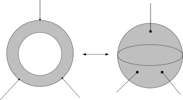
Figure 1: An open string one-loop amplitude (annulus) is dual to a closed string tree diagram (sphere).

One may think that the magic of deriving the $AdS$ spacetime structure from a free field theory comes from the simple structure of scalar fields, while in both ${\cal N}=4$ SYM and Supergravity theories, we have more complicated objects (even in free limit) and investigation of the duality via correlators remains non-obvious. An interesting early work on the correspondence of non-obvious correlators is [31] (see also [32]), where two and three point correlators of R-symmetry currents in ${\cal N}=4$ super Yang-Mills theory were obtained and confirmed the $AdS/CFT$ correspondence. In this paper, we try to implement the ideas of [22] to R-currents, i.e. in the worldline formalism framework we use the procedure of introducing bulk to boundary propagators via parameter integrals of heat kernel in the two and three point $R$-current correlation functions in super Yang-Mills theory. The importance of $R$-currents, besides their rich structure as vector fields, comes from the fact that they, as well as scalar fields, are protected objects in ${\cal N}=4$ SYM theory by supersymmetry. This enables us to use them in the free field limit and trust our results in wider limits. However, we have to restrict ourselves to at most three-point function, since higher n-point functions require bulk to bulk propagators in the $AdS$ space which in turn requires the sum over all string states. In contrast, in three-point function the only relevant propagator is the bulk to boundary propagator and it is enough to consider the lowest string state for this propagator. The important result is that when one considers the one loop correlation in the SYM theory, it is possible to reparametrise it in the same fashion of delta to star in the electrical networks and find out an amplitude which corresponds to a tree diagram. This amplitude is of course the closed string sphere diagram and explicitly can be shown to correspond to an amplitude of the bulk theory.

This paper is organized as follows. In section 1 we introduce the R-currents in $SYM$ theory and use the basic results of worldline formalism to derive the two point functions. Then in section 2 we investigate the three point function. In section 3 we introduce the vector field theory in the $AdS$ theory and review the derivation of the R-current correlation functions from the bulk theory. Section 4 is devoted to bringing the results of worldline formalism and $AdS$ supergravity in agreement with each other and we conclude in section 5. A very brief review on the worldline formalism is given the appendix.

1 R-currents in the SYM theory:two-point correlation functions

Let us start with the ${\cal N}=4$ super Yang-Mills theory which is given by the following action:

$$S = {\rm Tr}\int d^{4}x\frac{1}{4}F_{\mu\nu}F^{\mu\nu}-\frac{i}{2}\overline{\psi}_{a}\gamma^{\mu}D_{\mu}\psi^{a}-{\frac{1}{2}}D_{\mu}\phi_{ab}D^{\mu}\phi^{ab}$$ (1.1)

$$-\frac{i}{2}\overline{\psi}_{a}[\phi^{ab},\psi_{a}]+\frac{1}{4}[\phi_{ab},\phi_{cd}][\phi^{ab},\phi^{cd}]\;,$$

where $\mu,\nu=1,...,4$ are 4-dimensional space-time indices and $a,b=1,...,6$ are the internal directions. Under the R-symmetry fermions transform chirally in the fundamental representation 4 of $SU(4)$ and scalars transform as antisymmetric 6,

$$\delta\psi^{a}=\epsilon^{A}(T_{A})^{a}_{b}\frac{(1+\gamma_{5})}{2}\psi^{b},\;\;\;\;\delta\phi_{ab}=\epsilon^{A}(T_{A})_{ab}^{cd}\phi_{cd}$$

Then the corresponding global $SU(4)$ R-currents can be derived as,

$$J^{\mu}_{a}={\frac{1}{2}}\phi(x)T_{a}^{\phi}(\partial^{\mu}+A^{\mu}(x))\phi(x)-\frac{i}{2}\overline{\psi}(x)T_{a}^{\psi}\gamma^{\mu}\frac{(1+\gamma_{5})}{2}\psi(x).$$ (1.2)

Our aim is to find two and three point correlation functions for these R-currents which will be later interpreted as open string amplitude then in the following sections we will show that these can be transformed to closed string amplitudes. This transformation would be a realization of the open/closed string duality. In this regard, it is helpful to use the worldline formalism which in turn is a stringy inspired method in quantum field theory [17]. Indeed this formalism is the first quantization (in contrast to second quantization in the field theory) and so is comparable to the perturbative string theory.

The one-loop $N$-point R-current amplitude has contributions from both scalar and spinor loops as demonstrated in the diagram of Fig. 2.

Figure 2: The Feynmann diagram for $N$ point function of vector fields (dashed lines) evaluated by a scalar or spinor loop. $k_{i}$’s and $\epsilon_{i}$’s are the momenta and polarizations of vector fields, respectively. $u_{i}$’s are the insertion points on the worldline loop.

The scalar loop contribution to the $N$-point amplitude in $d=4-\epsilon$ dimension can be derived in the worldline formalism as [16]:

$$\Gamma_{N}\left(k_{1},...,k_{N}\right)=\frac{\left(ig\right)^{N}}{\left(4\pi\right)^{2}}Tr\left(T^{a_{N}}...T^{a_{1}}\right)\int\limits_{0}^{\infty}\frac{d\tau}{\tau^{3-N-\epsilon/2}}\int\limits_{0}^{1}du_{N-1}\int\limits_{0}^{u_{N-1}}du_{N-2}\dots\int\limits_{0}^{u_{2}}du_{1}$$

$$\times\exp\left[\sum\limits_{i<j=1}^{N}\left(k_{i}\cdot k_{j}G_{B}^{ji}-i\left(k_{i}\cdot\epsilon_{j}-k_{j}\cdot\epsilon_{i}\right)\stackrel{{\scriptstyle.}}{{G}}_{B}^{ji}+\epsilon_{i}\cdot\epsilon_{j}\stackrel{{\scriptstyle..}}{{G}}_{B}^{ji}\right)\right]\mid_{linear\ in\ each\ \epsilon}.$$ (1.3)

Here $\tau$ is the Schwinger proper-time and $u_{i}$ are parameters ordered in worldline loop $u_{N}\geq u_{N-1}\geq...\geq u_{1}$, $\epsilon_{i},$ and $k_{i},$ are polarization vectors and momenta of incoming and outgoing vector fields (gluons). The order of color $T^{a}$ matrices under the trace should be the same as the order of $u_{i}$ parameters, which is determined by positions of vector currents on the loop.

Spinor loop contribution, for the above ordering, is given by:

$$\Gamma_{N}\left(k_{1},...,k_{N}\right)=-2\frac{\left(ig\right)^{N}}{\left(4\pi\right)^{2}}Tr\left(T^{a_{N}}...T^{a_{1}}\right)\int\limits_{0}^{\infty}\frac{d\tau}{\tau^{3-N-\epsilon/2}}\int\limits_{0}^{1}du_{N-1}\int\limits_{0}^{u_{N-1}}du_{N-2}...\int\limits_{0}^{u_{2}}du_{1}$$

$$\times\exp\left[\sum\limits_{i<j=1}^{N}k_{i}\cdot k_{j}G_{B}^{ji}\right]\left\{\prod\limits_{i=1}^{N}\int d\theta_{i}d\overline{\theta}_{i}\exp\left[\sum\limits_{i<j=1}^{N}\left(-i\left(\overline{\theta}_{j}\theta_{j}k_{i}\cdot\epsilon_{j}-\overline{\theta}_{i}\theta_{i}k_{j}\cdot\epsilon_{i}\right)\stackrel{{\scriptstyle.}}{{G}}_{B}^{ji}\right.\right.\right.$$

$$\left.\left.\left.+\overline{\theta}_{i}\theta_{i}\overline{\theta}_{j}\theta_{j}\epsilon_{i}\cdot\epsilon_{j}\stackrel{{\scriptstyle..}}{{G}}_{B}^{ji}\right)+\left(-\overline{\theta}_{i}\overline{\theta}_{j}k_{i}\cdot k_{j}+i\overline{\theta}_{i}\theta_{j}k_{i}\cdot\epsilon_{j}+i\theta_{i}\overline{\theta}_{j}\epsilon_{i}\cdot k_{j}+\theta_{i}\theta_{j}\epsilon_{i}\cdot\epsilon_{j}\right)G_{F}^{ji}\right]\right\}$$ (1.4)

where $\theta,\overline{\theta}$ are Grassmann variables and bosonic and fermionic worldline Green’s functions are defined in the loop as:

$$G_{B}^{ji}\equiv\left(\left|\tau_{j}-\tau_{i}\right|-\frac{1}{\tau}\left(\tau_{j}-\tau_{i}\right)^{2}\right)=\tau\left(\left|u_{j}-u_{i}\right|-\left(u_{j}-u_{i}\right)^{2}\right),$$

$$G_{F}^{ji}=sign\left(\tau_{j}-\tau_{i}\right),$$

with $\tau_{i}=u_{i}\tau$. Notice, that formulas (1.3) and (1.4) do not contain the self interaction of vector field, which leads to one-particle reducible diagrams. So, here we are going to consider only contribution of one-particle irreducible diagrams. The first and second derivatives of worldline Green’s function $G_{B}^{ji}$ are:

$$\frac{\partial}{\partial\tau^{j}}G_{B}^{ji}=\stackrel{{\scriptstyle.}}{{G}}_{B}^{ji}=sign\left(\alpha^{j}-\alpha^{i}\right)\left(1-2\left|\epsilon^{ijk}\right|\alpha_{k}\right)=\left(-1\right)^{F_{ij}}\left(1-2\left|\epsilon^{ijk}\right|\alpha_{k}\right),$$ (1.5)

$$\frac{\partial^{2}}{\left(\partial\tau^{j}\right)^{2}}G_{B}^{ji}=\stackrel{{\scriptstyle..}}{{G}}_{B}^{ji}=\frac{2}{\tau}\left(\left|\epsilon^{ijk}\right|\delta\left(\alpha_{k}\right)-1\right),$$ (1.6)

Here $\alpha_{i}=|u_{i}-u_{i+1}|$, $\epsilon^{ijk}$ is unit antisymmetric tensor and $\left(-1\right)^{F_{ij}}$ replaces the signature function above: $F_{ij}=\left\{\begin{array}[]{c}1\ for\ j<i\\ 0\ for\ j>i\end{array}\right.$.

Beside the scalar and spinor loops, in super Yang-Mills theory there is a vector field loop. However since we are working in the free field limit, it doesn’t contribute.

Now let us concentrate on two-point function of vector fields which is known in literature as polarization operator (photon or gluon). Worldline expression of scalar loop contribution to this function can be obtained from (1.3), with $N=2$. After little simplification it gets the following form, which coincides with the ordinary expression in Schwinger’s proper time parameter [16]:

$$\Pi^{ab}_{{\rm scalar}}\left(k_{1},k_{2}\right) =- Tr\left(T^{a}T^{b}\right)\frac{\left(g\mu^{\epsilon/2}\right)^{2}}{\left(4\pi\right)^{2-\epsilon/2}}\int\limits_{0}^{\infty}\frac{d\tau}{\tau^{d/2-1}}\int\limits_{0}^{1}d\alpha\ e^{\tau k_{1}k_{2}\alpha\left(1-\alpha\right)}\int\limits_{-\infty}^{\infty}\frac{d^{d}z}{\left(2\pi\right)^{d}}e^{i\left(k_{1}+k_{2}\right)z}$$ (1.7)

$$\times\left[\frac{2}{\tau}\left(\delta\left(\alpha\right)-1\right)\epsilon_{1}\cdot\epsilon_{2}+\left(1-2\alpha\right)^{2}\left(\epsilon_{1}\cdot k_{2}\right)\left(\epsilon_{2}\cdot k_{1}\right)\right]\;.$$

The last integral means the energy-momentum conservation. Remind that the polarization operator (1.7) contains contribution of tadpole diagram of vector-scalar interaction in $\delta\left(\alpha\right)$-function term. It differs from two-point correlation function of free scalar field only by additional square bracket factor in it [16, 15]. Now the next step is going to position space by means of the inverse Fourier transformation:

$$\Pi^{ab}_{{\rm scalar}}\left(x_{1},x_{2}\right)=-Tr\left(T^{a}T^{b}\right)C\int\limits_{0}^{\infty}\frac{d\tau}{\tau^{d/2-1}}\int\limits_{-\infty}^{\infty}d^{d}k_{1}\int\limits_{-\infty}^{\infty}d^{d}k_{2}\int\limits_{-\infty}^{\infty}\frac{d^{d}z}{\left(2\pi\right)^{d}}e^{i\left(k_{1}+k_{2}\right)z}\textsl{}$$

$$\times\int\limits_{0}^{1}d\alpha\ \int\limits_{0}^{1}d\beta\ e^{-\tau k_{1}^{2}\beta\alpha\left(1-\alpha\right)-\tau k_{2}^{2}\left(1-\beta\right)\alpha\left(1-\alpha\right)}e^{-ik_{1}x_{1}-ik_{2}x_{2}}$$

$$\times\left[\frac{2}{\tau}\left(\delta\left(\alpha\right)-1\right)\epsilon_{1}\cdot\epsilon_{2}+\left(1-2\alpha\right)^{2}\left(\epsilon_{1}\cdot\left(i\frac{\partial}{\partial x_{2}}\right)\right)\left(\epsilon_{2}\cdot\left(i\frac{\partial}{\partial x_{1}}\right)\right)\right]$$ (1.8)

Here we have inserted an integral over the parameter $\beta$, where $0\leq\beta\leq 1$. Taking Gaussian integrals over the momenta and then position derivatives, we obtain from (1.8) the following expression of polarization operator:

$$\Pi^{ab}_{{\rm scalar}}\left(x_{1},x_{2}\right) = -CTr\left(T^{a}T^{b}\right)\int\limits_{0}^{\infty}\frac{d\tau}{\tau^{d/2-1}}\int\limits_{0}^{1}d\alpha\ \int\limits_{0}^{1}d\beta\ \int\limits_{-\infty}^{\infty}d^{d}z\ \left(\frac{\pi}{\tau\beta\alpha\left(1-\alpha\right)}\right)^{d/2}$$

$$\times e^{-\frac{\left(z-x_{1}\right)^{2}}{4\tau\beta\alpha\left(1-\alpha\right)}}\left(\frac{\pi}{\tau\left(1-\beta\right)\alpha\left(1-\alpha\right)}\right)^{d/2}e^{-\frac{\left(z-x_{2}\right)^{2}}{4\tau\left(1-\beta\right)\alpha\left(1-\alpha\right)}}\left[\frac{2}{\tau}\left(\delta\left(\alpha\right)-1\right)\epsilon_{1}\cdot\epsilon_{2}\right.$$

$$\left.-\left(1-2\alpha\right)^{2}\frac{1}{2\tau\left(1-\beta\right)\alpha\left(1-\alpha\right)}\epsilon_{1}\cdot\left(z-x_{2}\right)\frac{1}{2\tau\beta\alpha\left(1-\alpha\right)}\epsilon_{2}\cdot\left(z-x_{1}\right)\right].$$

Writing the exponents in heat kernel terms by means of:

$$\left(\frac{1}{4\pi t}\right)^{d/2}\ e^{-\frac{\left(x-z\right)^{2}}{4t}}=\left\langle x\left|e^{t\Box}\right|z\right\rangle,$$ (1.10)

we rewrite (1) as follows:

$$\Pi^{ab}_{{\rm scalar}}\left(x_{1},x_{2}\right)=-C^{\prime}Tr\left(T^{a}T^{b}\right)\int\limits_{0}^{\infty}\frac{d\tau}{\tau^{d/2-1}}\int\limits_{0}^{1}d\alpha\ \int\limits_{0}^{1}d\beta\ \int\limits_{-\infty}^{\infty}d^{d}z\left\langle x_{1}\left|e^{\tau\beta\alpha\left(1-\alpha\right)\Box}\right|z\right\rangle\times\\$$

$$\left\langle x_{2}\left|e^{\tau\left(1-\beta\right)\alpha\left(1-\alpha\right)\Box}\right|z\right\rangle\left[\frac{2}{\tau}\left(\delta\left(\alpha\right)-1\right)\epsilon_{1}\cdot\epsilon_{2}-\left(1-2\alpha\right)^{2}\frac{\epsilon_{1}\cdot\left(z-x_{2}\right)}{2\tau\alpha\left(1-\beta\right)\left(1-\alpha\right)}\frac{\epsilon_{2}\cdot\left(z-x_{1}\right)}{2\tau\beta\alpha\left(1-\alpha\right)}\right].\\$$

We can insert the integral representation of $\Gamma\left(s\right)$ function,

$$1=\frac{1}{\Gamma\left(d/2\right)}\int\limits_{0}^{\infty}d\rho\rho^{d/2-1}e^{-\rho}=\frac{1}{\Gamma\left(d/2+1\right)}\int\limits_{0}^{\infty}d\rho\rho^{d/2}e^{-\rho},$$ (1.11)

into (1) and pass to new variables [22]:

$$\rho_{1}=\rho\left(1-\beta\right),\ \rho_{2}=\beta\rho\;\;\;{\rm and}\;\;\;t=4\tau\rho\beta\left(1-\beta\right)\alpha\left(1-\alpha\right).$$

with $\int\limits_{0}^{\infty}\rho d\rho\int\limits_{0}^{1}d\beta=\int\limits_{0}^{\infty}d\rho_{1}\int\limits_{0}^{\infty}d\rho_{2}$, then the polarization operator (1) is rewritten in a more symmetric form:

$$\Pi^{ab}_{{\rm scalar}}\left(x_{1},x_{2}\right)=\int\limits_{0}^{\infty}\frac{dt}{t^{\frac{d}{2}+1}}\ \int\limits_{-\infty}^{\infty}d^{d}z\int\limits_{0}^{\infty}d\rho_{1}\rho_{1}^{\frac{d}{2}-1}e^{-\rho_{1}}\left\langle x_{1}\left|e^{\frac{t}{4\rho_{1}}\Box}\right|z\right\rangle\int\limits_{0}^{\infty}d\rho_{2}\rho_{2}^{\frac{d}{2}-1}e^{-\rho_{2}}\left\langle x_{2}\left|e^{\frac{t}{4\rho_{2}}\Box}\right|z\right\rangle\\$$

$$\times\left[-\frac{C^{ab}_{1}}{\Gamma\left(d/2+1\right)}t\epsilon_{1}\cdot\epsilon_{2}+\frac{C^{ab}_{2}}{\Gamma\left(d/2\right)}\epsilon_{1}\cdot\left(z-x_{2}\right)\epsilon_{2}\cdot\left(z-x_{1}\right)\right].$$ (1.12)

Here we have taken into account $\rho_{1}+\rho_{2}=\rho$ in the exponent and have included integrals over the $\alpha$ into constants $C_{1,2}^{ab}$:

$$\begin{array}[]{c}C^{ab}_{1}=Tr\left(T^{a}T^{b}\right)4^{d/2-1}C^{\prime}\int\limits_{0}^{1}d\alpha\ \left[\alpha\left(1-\alpha\right)\right]^{d/2-1}\left(\delta\left(\alpha\right)-1\right),\\ C^{ab}_{2}=Tr\left(T^{a}T^{b}\right)4^{d/2-2}C^{\prime}\int\limits_{0}^{1}d\alpha\ \left[\alpha\left(1-\alpha\right)\right]^{d/2-2}\left(1-2\alpha\right)^{2},\\ C^{\prime}=g^{2}\mu^{4-d}2^{d/2-6}\left(2\pi\right)^{d/2-4}\end{array}$$

Note that , the $\Gamma\left(s\right)$ function arises here naturally, as a well-known correction (using generalized $\zeta-$ function in [27] and other approaches) to the one-loop effective action. Following [22] we separate the integrals over the $\rho_{i}$, which contain heat kernel, and denote them by the $K_{1}\left(x_{i},z,t\right)$ function:

$$K_{1}\left(x_{i},z,t\right)=\int\limits_{0}^{\infty}d\rho_{i}\rho_{i}^{d/2-1}e^{-\rho_{i}}\left\langle x_{i}\left|e^{\frac{t}{4\rho_{i}}\Box}\right|z\right\rangle.$$ (1.13)

Given the $AdS$ metric as $ds^{2}=(dz_{0}^{2}+d\vec{z}^{2})/z_{0}^{2}$, it can be shown that the function $K_{1}\left(x_{i};z,t\right)$ obeys the $d+1$-dimensional massless Klein-Gordon equation in the $AdS$ background:

$$\left[-z_{0}^{2}\partial_{z_{0}}^{2}+\left(d-1\right)z_{0}\partial_{z_{0}}-z_{0}^{2}\Box\right]K_{1}\left(x;z,t\right)=0,$$ (1.14)

where $t=z_{0}^{2}$ and $\Box$ is the $d$-dimensional Laplacian in directions $\overrightarrow{z}$. The physical interpretation of the function $K_{1}\left(x_{i},z,t\right)$ is the bulk to boundary propagator of massless vector field in the $d+1$-dimensional $AdS$ spacetime with the radial coordinate $t=z_{0}^{2}$. Now we can write (1) in terms of this propagator in a more suitable form to match with the two-point supergravity correlator (3.7):

$$\Pi^{ab}_{{\rm scalar}}\left(x_{1},x_{2}\right) = \int\limits_{0}^{\infty}\frac{dt}{t^{d/2+1}}\int\limits_{-\infty}^{\infty}d^{d}z\ K_{1}\left(x_{1};z,t\right)K_{1}\left(x_{2};z,t\right)$$ (1.15)

$$\times\left[-\frac{C^{ab}_{1}}{\Gamma\left(\frac{d}{2}+1\right)}\epsilon_{1}\cdot\epsilon_{2}t+\frac{C^{ab}_{2}}{\Gamma\left(\frac{d}{2}\right)}\epsilon_{1}\cdot\left(z-x_{2}\right)\epsilon_{2}\cdot\left(z-x_{1}\right)\right].$$

Comparing (1.15) with the two-point correlation function $\Gamma\left(x_{1},x_{2}\right)$ for free scalar field theory, we find the additional square bracket factor in our case, which should be replaced by $t^{3}$ for free scalar theory. Thus, the gluon polarization operator is expressed in terms of bulk to boundary propagator $K_{1}\left(x;z,t\right)$ of a massless field.

For vector-spinor interaction case we have spinor particles in the loop and the two-point function is obtained from the one loop spinor effective action. Setting $N=2$ in (1.4) and taking integrals over the Grassmann variables, it gets the following form [16]:

$$\Pi^{ab}_{{\rm spinor}}\left(k_{1},k_{2}\right)=2Tr\left(T^{a}T^{b}\right)\frac{\left(g\mu^{\epsilon/2}\right)^{2}}{\left(4\pi\right)^{2-\epsilon/2}}\int\limits_{0}^{\infty}\frac{d\tau}{\tau^{d/2-1}}\int\limits_{0}^{1}d\alpha\ e^{\tau k_{1}k_{2}\alpha\left(1-\alpha\right)}\int\limits_{-\infty}^{\infty}\frac{d^{d}z}{\left(2\pi\right)^{d}}e^{i\left(k_{1}+k_{2}\right)z}\\$$

$$\times\left[\frac{2}{\tau}\left(\delta\left(\alpha\right)-1\right)\epsilon_{1}\cdot\epsilon_{2}+\left[\left(1-2\alpha\right)^{2}-1\right]\left(\epsilon_{1}\cdot k_{2}\right)\left(\epsilon_{2}\cdot k_{1}\right)+\left(\epsilon_{1}\cdot\epsilon_{2}\right)\left(k_{1}\cdot k_{2}\right)\right].$$ (1.16)

The worldline expression of two-point correlator for this interaction has minor difference with the scalar loop case in square bracket in (1.7) [17, 27]. This enables us to re-express the spinor loop case in (1) similar to (1.15) as:

$$\Pi^{ab}_{{\rm spinor}}\left(x_{1},x_{2}\right)=2\int\limits_{0}^{\infty}\frac{dt}{t^{d/2+1}}\int\limits_{-\infty}^{\infty}d^{d}z\ K_{1}\left(x_{1};z,t\right)K_{1}\left(x_{2};z,t\right)\left[C^{ab}_{1}\frac{1}{\Gamma\left(d/2+1\right)}\epsilon_{1}\cdot\epsilon_{2}t\right.+\\$$

$$\left.+\frac{1}{\Gamma\left(d/2\right)}\ \left[C^{ab}_{2}\epsilon_{1}\cdot\left(z-x_{2}\right)\epsilon_{2}\cdot\left(z-x_{1}\right)-C^{ab}_{3}\epsilon_{1}\cdot\epsilon_{2}\left(z-x_{1}\right)\cdot\left(z-x_{2}\right)\right]\right].$$ (1.17)

$$C^{ab}_{3}=Tr\left(T^{a}T^{b}\right)C^{\prime}\int\limits_{0}^{1}d\alpha\ \left[\alpha\left(1-\alpha\right)\right]^{d/2-2}$$

Thus, we see from (1.15) and (1) that in $AdS$ space the two-point correlators of massless vector field interacted with the scalar and spinor fields are expressed by means of massless bulk to boundary propagator in this spacetime.

Before adding the contributions of scalar and fermion loops, we should recall that our fermions are in ${\bf 4}$ and scalars are in ${\bf 6}$ representations of $SU(4)$ group, they have $1/2$ and $1$ quadratic casimir, respectively. So we add 2 times of scalar loop contribution to the fermion one to find:

$$\Pi^{ab}\left(x_{1},x_{2}\right)=4C_{2}\frac{1}{\Gamma\left(d/2\right)}\epsilon_{1}^{i}\epsilon_{2}^{j}\int\limits_{0}^{\infty}\frac{dt}{t^{d/2+1}}\int d^{d}z\ K_{1}\left(x_{1}\right)K_{1}\left(x_{2}\right)$$

$$\times\left[\left(z-x_{1}\right)_{i}\left(z-x_{2}\right)_{j}-\delta_{ij}\left(z-x_{1}\right)\cdot\left(z-x_{2}\right)\right].$$ (1.18)

As we will see later, the above result can be interpreted as a correlation obtained in the bulk theory, where $K_{1}$ functions are the bulk to boundary propagators and the square bracket show the tensorial structure. We will be back on this in section 4.

2 The three-point function

At one loop approximation the field theory three-point correlation function is the loop (scalar or spinor) having three external vector field lines. Physically it describes photon or gluon splitting amplitude due to the Dirac vacuum of spinor (scalar) particles. According to Furry’s theorem in QED an amplitude with an odd number of external vector lines is zero in absence of background fields [28, 17]. In non-abelean theory it becomes non-zero due to color matrices in the internal lines. The starting expression for scalar loop contribution to three-point correlation function of non-abelean vector field can be found from (1.3) by setting $N=3$, and changing variables $\alpha_{i}=\left|u_{i}-u_{i+1}\right|$:

$$\Gamma^{abc}\left(k_{1},k_{2},k_{3}\right)=Tr\left(T^{a}T^{b}T^{c}\right)\frac{\left(ig\mu^{\epsilon/2}\right)^{3}}{\left(4\pi\right)^{2-\epsilon/2}}\delta^{\left(d\right)}\left(\sum k_{l}\right)\int\limits_{0}^{\infty}\frac{d\tau}{\tau^{d/2-2}}\prod\limits_{l=1}^{3}\int\limits_{0}^{1}d\alpha_{l}\delta\left(\sum\alpha_{l}-1\right)$$

$$\times\ e^{-\tau\left(k_{1}^{2}\alpha_{2}\alpha_{3}+k_{2}^{2}\alpha_{1}\alpha_{3}+k_{3}^{2}\alpha_{1}\alpha_{2}\right)}\left[\exp\sum\limits_{i<j}\left[-i\left(k_{i}\cdot\epsilon_{j}-k_{j}\cdot\epsilon_{i}\right)\stackrel{{\scriptstyle.}}{{G}}_{B}^{ji}+\epsilon_{i}\cdot\epsilon_{j}\stackrel{{\scriptstyle..}}{{G}}_{B}^{ji}\right]\right]\mid_{linear\ in\ each\ \epsilon},$$ (2.1)

Here in the first exponent we have used $k_{i}\cdot k_{j}=\frac{1}{2}\left({k_{k}}^{2}-{k_{i}}^{2}-{k_{j}}^{2}\right)$, that is the result of the energy-momentum conservation. The above amplitude is distinct from the three-point correlation function for the free scalar field theory by an additional square bracket factor [22]. Decomposing this square bracket and keeping the terms which have only first degree of each $\epsilon_{i}$ , we get the following expression for this bracket:

$$-i\sum\limits_{i<j}\left(\epsilon_{i}\cdot\epsilon_{j}\stackrel{{\scriptstyle..}}{{G}}_{B}^{ji}+k_{i}\cdot\epsilon_{j}k_{j}\cdot\epsilon_{i}\left(\stackrel{{\scriptstyle.}}{{G}}_{B}^{ji}\right)^{2}\right)\left(k_{i}\cdot\epsilon_{k}\stackrel{{\scriptstyle.}}{{G}}_{B}^{ki}+k_{j}\cdot\epsilon_{k}\stackrel{{\scriptstyle.}}{{G}}_{B}^{kj}\right)\\$$

$$-i\sum\limits_{i<j,k}k_{i}\cdot\epsilon_{j}\ k_{j}\cdot\epsilon_{k}k_{k}\cdot\epsilon_{i}\stackrel{{\scriptstyle.}}{{G}}_{B}^{ij}\stackrel{{\scriptstyle.}}{{G}}_{B}^{jk}\stackrel{{\scriptstyle.}}{{G}}_{B}^{ki}$$ (2.2)

Going to the position space by Fourier transformation we integrate over the momenta and write the result in the heat kernel terms using (1.10):

$$\int dk_{i}\ \exp\left\{-\tau k_{i}^{2}\alpha_{j}\alpha_{k}+ik_{i}\left(z-x_{i}\right)\right\}=$$

$$\left(\frac{\pi}{\tau\alpha_{j}\alpha_{k}}\right)^{1/2}\exp\left\{-\frac{\left(z-x_{i}\right)^{2}}{4\tau\alpha_{j}\alpha_{k}}\right\}=\left(2\pi\right)^{d}\left\langle z\left|e^{\tau\alpha_{j}\alpha_{k}\Box}\right|x_{i}\right\rangle.$$

In square bracket factor we replace momenta as follows: $k_{j}\rightarrow\left(i\frac{\partial}{\partial x_{j}}\right)\rightarrow-i\frac{\left(x_{j}-z\right)}{2\tau\alpha_{i}\alpha_{k}}$. Integrals over the $\alpha_{i}$ in position space will have the form:

$$\int\limits_{0}^{\infty}d\tau\frac{1}{\tau^{d/2-2}}\int\limits_{0}^{1}d\alpha_{1}\int\limits_{0}^{1}d\alpha_{2}\int\limits_{0}^{1}d\alpha_{3}\delta\left(\sum\alpha_{i}-1\right)\int d^{d}z\prod\limits_{i=1}^{3}\left\langle x_{i}\left|e^{\tau\alpha_{j}\alpha_{k}\Box}\right|z\right\rangle.$$ (2.3)

For three-point function the change of variables is the following one [22]:

$$t=4\tau\alpha_{1}\alpha_{2}\alpha_{3}\rho,\ \tau\alpha_{j}\alpha_{k}=\frac{t}{4\rho_{i}},\ \rho_{i}=\rho\alpha_{i}.$$

Then the integral (2.3) changes to:

$$4^{d/2-3}\int\limits_{0}^{\infty}\frac{dt}{t^{d/2-2}}\ \rho^{-d+4}\prod\limits_{i=1}^{3}\int\limits_{0}^{\rho}d\rho_{i}\ \rho_{i}^{d/2-3}\delta\left(\sum\rho_{i}-\rho\right)\int d^{d}z\left\langle x_{i}\left|e^{\frac{t}{4\rho_{i}}\Box}\right|z\right\rangle$$

In these variables $\stackrel{{\scriptstyle.}}{{G}}_{B}^{ij}$, $\stackrel{{\scriptstyle..}}{{G}}_{B}^{ij}$ and momenta can be written as:

$$\stackrel{{\scriptstyle.}}{{G}}_{B}^{ij}=\left(-1\right)^{F_{ij}}\left(1-2\rho^{-1}\rho_{k}\right),\ \stackrel{{\scriptstyle..}}{{G}}_{B}^{ij}=\frac{8\rho^{-2}}{t}\prod\limits_{l=1}^{3}\rho_{l}\left(\rho\delta\left(\rho_{k}\right)-1\right),\ k_{i}\rightarrow-i\frac{2\rho_{i}}{t}\left(z-x_{i}\right).$$

Taking these expressions into account in (2.2), the additional square bracket factor has the following explicit form in the new variables $\rho_{i}$ and $\ t$:

$$-\frac{8}{t^{2}}\prod\limits_{l=1}^{3}\rho_{l}\sum\limits_{i<j}\left[2\rho^{-2}\epsilon_{i}\cdot\epsilon_{j}+\frac{1}{t}\epsilon_{i}\cdot\left(z-x_{j}\right)\epsilon_{j}\cdot\left(z-x_{i}\right)\left(\rho_{k}^{-1}-4\rho^{-1}+4\rho^{-2}\rho_{k}\right)\right]$$

$$\times\left[\left(-1\right)^{F_{ik}}\epsilon_{k}\cdot\left(z-x_{i}\right)\rho_{i}\left(1-2\rho^{-1}\rho_{j}\right)+\left(-1\right)^{F_{jk}}\epsilon_{k}\cdot\left(z-x_{j}\right)\rho_{j}\left(1-2\rho^{-1}\rho_{i}\right)\right]$$

$$-\frac{8}{t^{3}}\prod\limits_{l=1}^{3}\rho_{l}\sum\limits_{i<j,k}\left(-1\right)^{F_{ij}+F_{ik}+F_{jk}}\epsilon_{i}\cdot\left(z-x_{k}\right)\epsilon_{k}\cdot\left(z-x_{j}\right)\epsilon_{j}\cdot\left(z-x_{i}\right)$$

$$\times\left[1-4\rho^{-2}\left(\rho_{i}\rho_{j}+\rho_{i}\rho_{k}+\rho_{k}\rho_{j}\right)+8\rho^{-3}\rho_{i}\rho_{j}\rho_{k}\right].$$ (2.4)

Notice that in (2.4) for three-point function we cannot factor out $\alpha$ -dependent integrals and introduce an integral over $\beta$, as we made for two-point function case, since here we have different degrees of $\rho_{i}$ and $\rho$. This means that we should introduce different $\Gamma\left(d-m\right)$ and $K_{n}\left(x,z,t\right)$ functions corresponding to these degrees of $\rho$ and $\rho_{i}$. So, the three-point function, in addition of $K_{1}$, includes $K_{2}$ and $K_{3}$ functions which are defined as:

$$\begin{array}[]{c}K_{n}\left(x_{i},z,t\right)\equiv\int\limits_{0}^{\infty}d\rho_{i}\rho_{i}^{d/2-n}e^{-\rho_{i}}\left\langle x_{i}\left|e^{\frac{t}{4\rho_{i}}\Box}\right|z\right\rangle.\end{array}$$ (2.5)

The appearance of these functions in the three-point function is the reflection of derivative interactions in the bulk theory. Indeed,

$$\frac{\partial K_{n}}{\partial x^{\mu}}=-\frac{2}{t}(x^{\mu}-z^{\mu})K_{n-1}$$

Thereby, rewritten in terms of $K_{n}\left(x_{i}\right)$ functions the three-point correlation function (2) will have the following form:

$$\Gamma^{abc}\left(x_{1},x_{2},x_{3}\right)=\frac{i2^{d/2-3}\left(g\mu^{\epsilon/2}\right)^{3}}{\left(2\pi\right)^{3/2}}Tr\left(T^{a}T^{b}T^{c}\right)\int\limits_{0}^{\infty}\frac{dt}{t^{d/2+1}}\int\limits_{-\infty}^{\infty}d^{d}z\ \left[\sum\limits_{i<j}\left\{\left(z-x_{i}\right)\cdot\epsilon_{k}\times\right.\right.$$

$$\left[\left(-1\right)^{F_{ik}}\cdot K_{1}\left(x_{i}\right)K_{2}\left(x_{j}\right)+\left(-1\right)^{F_{jk}}K_{1}\left(x_{j}\right)K_{2}\left(x_{i}\right)\right]\left[\frac{2}{\Gamma\left(d-1\right)}t\epsilon_{i}\cdot\epsilon_{j}K_{2}\left(x_{k}\right)+\right.$$

$$\left.\left(z-x_{i}\right)\cdot\epsilon_{j}\left(z-x_{j}\right)\cdot\epsilon_{i}\left(\frac{1}{\Gamma\left(d-3\right)}K_{3}\left(x_{k}\right)-\frac{4}{\Gamma\left(d-2\right)}K_{2}\left(x_{k}\right)+\frac{4}{\Gamma\left(d-1\right)}K_{1}\left(x_{k}\right)\right)\right]$$

$$-2\left(\left(-1\right)^{F_{ik}}+\left(-1\right)^{F_{jk}}\right)\left(z-x_{i}\right)\cdot\epsilon_{k}\left[\frac{2}{\Gamma\left(d\right)}t\epsilon_{i}\cdot\epsilon_{j}K_{2}\left(x_{k}\right)+\right.$$

$$\left.\left.\left(z-x_{i}\right)\cdot\epsilon_{j}\left(z-x_{j}\right)\cdot\epsilon_{i}\left(\frac{1}{\Gamma\left(d-2\right)}K_{3}\left(x_{k}\right)-\frac{4}{\Gamma\left(d-1\right)}K_{2}\left(x_{k}\right)+\frac{4}{\Gamma\left(d\right)}K_{1}\left(x_{k}\right)\right)\right]\right\}$$

$$+\sum\limits_{i<j,k}\left(-1\right)^{F_{jk}}\left(z-x_{i}\right)\cdot\epsilon_{j}\left(z-x_{j}\right)\cdot\epsilon_{k}\left(z-x_{k}\right)\cdot\epsilon_{i}\left\{\frac{1}{\Gamma\left(d-3\right)}K_{2}\left(x_{i}\right)K_{2}\left(x_{j}\right)K_{2}\left(x_{k}\right)\right.$$

$$-\frac{4}{\Gamma\left(d-1\right)}\left[K_{2}\left(x_{i}\right)K_{1}\left(x_{j}\right)K_{1}\left(x_{k}\right)+K_{1}\left(x_{i}\right)K_{2}\left(x_{j}\right)K_{1}\left(x_{k}\right)+K_{1}\left(x_{i}\right)K_{1}\left(x_{j}\right)K_{2}\left(x_{k}\right)\right]$$

$$\left.\left.+\frac{8}{\Gamma\left(d\right)}K_{1}\left(x_{i}\right)K_{1}\left(x_{j}\right)K_{1}\left(x_{k}\right)\right\}\right]$$ (2.6)

As is seen here, the three-point correlation function is expressed by means of bulk to boundary propagators of massless fields and its descendants. This is in contrast to the free scalar field theory where the three-point correlation function was expressed in terms of a unique bulk to boundary propagator of a massive scalar field [22]. From the $AdS/CFT$ correspondence dictionary, we expect the appearance of the massless propagator, $K_{1}$, as it happened in the two-point function. Indeed, $K_{2}$ and $K_{3}$ functions are not really independent propagators and their appearance, as mentioned before, is due to derivative interactions.

The fermionic loop contribution to the three-point function of non-abelean vector field is not zero. This is in contrast to the abelean theory, where contribution of one-loop diagrams with odd number vertices vanishes due to Furry’s theorem. The contribution of this loop can be obtained from formula (1.4) by setting $N=3$ . Decomposing the exponent, keeping only the terms linear in each $\epsilon$ and then taking integrals over the Grassmann variables we obtain:

$$\Gamma^{abc}\left(k_{1},k_{2},k_{3}\right)=-2\frac{\left(ig\right)^{3}}{\left(4\pi\right)^{2}}Tr\left(T^{a}T^{b}T^{c}\right)\int\limits_{0}^{\infty}d\tau\ \prod\limits_{l=1}^{3}\int\limits_{0}^{1}d\alpha_{l}\ e^{-\tau\left(k_{1}^{2}\alpha_{2}\alpha_{3}+k_{2}^{2}\alpha_{1}\alpha_{3}+k_{3}^{2}\alpha_{1}\alpha_{2}\right)}$$

$$\times\delta\left(\sum k_{i}\right)\delta\left(\sum\alpha_{i}-1\right)\left(-i\right)\left[{\rm scalar\ loop\ terms\ }+\left(k_{1}\cdot k_{2}\ \epsilon_{1}\cdot\epsilon_{2}-k_{1}\cdot\epsilon_{2}\ \ k_{2}\cdot\epsilon_{1}\right)\times\right.$$

$$\left(k_{1}\cdot\epsilon_{3}\stackrel{{\scriptstyle.}}{{G}}_{B}^{31}+k_{2}\cdot\epsilon_{3}\stackrel{{\scriptstyle.}}{{G}}_{B}^{32}\ \right)+\left(k_{1}\cdot k_{3}\ \epsilon_{1}\cdot\epsilon_{3}-k_{1}\cdot\epsilon_{3}\ \ k_{3}\cdot\epsilon_{1}\right)\left(k_{1}\cdot\epsilon_{2}\stackrel{{\scriptstyle.}}{{G}}_{B}^{21}-k_{3}\cdot\epsilon_{2}\stackrel{{\scriptstyle.}}{{G}}_{B}^{32}\ \right)$$

$$-\left(k_{2}\cdot k_{3}\ \epsilon_{2}\cdot\epsilon_{3}-k_{2}\cdot\epsilon_{3}\ k_{3}\cdot\epsilon_{2}\right)\left(k_{2}\cdot\epsilon_{1}\stackrel{{\scriptstyle.}}{{G}}_{B}^{21}+k_{3}\cdot\epsilon_{1}\stackrel{{\scriptstyle.}}{{G}}_{B}^{31}\ \right)+\left[\left(k_{1}\cdot\epsilon_{2}\ \epsilon_{1}\cdot\epsilon_{3}-\epsilon_{1}\cdot\epsilon_{2}\ \ k_{1}\cdot\epsilon_{3}\right)\right.$$

$$\times k_{2}\cdot k_{3}-\left(\epsilon_{1}\cdot k_{2}\ \ k_{1}\cdot k_{3}-k_{1}\cdot k_{2}\ \epsilon_{1}\cdot k_{3}\right)\epsilon_{2}\cdot\epsilon_{3}+\left(\epsilon_{1}\cdot\epsilon_{2}\ \ k_{1}\cdot k_{3}-k_{1}\cdot\epsilon_{2}\ \ k_{3}\cdot\epsilon_{1}\right)k_{2}\cdot\epsilon_{3}$$

$$\left.\left.-\left(k_{1}\cdot k_{2}\ \epsilon_{1}\cdot\epsilon_{3}-k_{1}\cdot\epsilon_{3}\ \ k_{2}\cdot\epsilon_{1}\right)k_{3}\cdot\epsilon_{2}\right]G_{F}^{21}G_{F}^{31}G_{F}^{32}\right]$$ (2.7)

Since our fermions are in ${\bf 4}$ and scalars are in ${\bf 6}$ representations of $SU(4)$ group, they have $1/2$ and $1$ quadratic casimir, respectively. So we should add 2 times of scalar loop contribution (2) to the fermionic loop contribution (2.7). Scalar loop terms again are canceled and in the square bracket only the following terms remain:

$$\left[\left(k_{1}\cdot k_{2}\ \epsilon_{1}\cdot\epsilon_{2}-k_{1}\cdot\epsilon_{2}\ \ k_{2}\cdot\epsilon_{1}\right)\left(k_{1}\cdot\epsilon_{3}\stackrel{{\scriptstyle.}}{{G}}_{B}^{31}+k_{2}\cdot\epsilon_{3}\stackrel{{\scriptstyle.}}{{G}}_{B}^{32}\ \right)+\left(k_{1}\cdot k_{3}\ \epsilon_{1}\cdot\epsilon_{3}-k_{1}\cdot\epsilon_{3}\ \ k_{3}\cdot\epsilon_{1}\right)\right.$$

$$\times\left(k_{1}\cdot\epsilon_{2}\stackrel{{\scriptstyle.}}{{G}}_{B}^{21}-k_{3}\cdot\epsilon_{2}\stackrel{{\scriptstyle.}}{{G}}_{B}^{32}\ \right)-\left(k_{2}\cdot k_{3}\ \epsilon_{2}\cdot\epsilon_{3}-k_{2}\cdot\epsilon_{3}\ k_{3}\cdot\epsilon_{2}\right)\left(k_{2}\cdot\epsilon_{1}\stackrel{{\scriptstyle.}}{{G}}_{B}^{21}+k_{3}\cdot\epsilon_{1}\stackrel{{\scriptstyle.}}{{G}}_{B}^{31}\ \right)$$

$$-\left[\left(k_{1}\cdot\epsilon_{2}\ \epsilon_{1}\cdot\epsilon_{3}-\epsilon_{1}\cdot\epsilon_{2}\ \ k_{1}\cdot\epsilon_{3}\right)k_{2}\cdot k_{3}-\left(\epsilon_{1}\cdot k_{2}\ \ k_{1}\cdot k_{3}-k_{1}\cdot k_{2}\ \epsilon_{1}\cdot k_{3}\right)\epsilon_{2}\cdot\epsilon_{3}+\right.$$

$$\left.\left.+\left(\epsilon_{1}\cdot\epsilon_{2}\ \ k_{1}\cdot k_{3}-k_{1}\cdot\epsilon_{2}\ \ k_{3}\cdot\epsilon_{1}\right)k_{2}\cdot\epsilon_{3}-\left(k_{1}\cdot k_{2}\ \epsilon_{1}\cdot\epsilon_{3}-k_{1}\cdot\epsilon_{3}\ \ k_{2}\cdot\epsilon_{1}\right)k_{3}\cdot\epsilon_{2}\right]\right].$$ (2.8)

In position space with $d=4$ by repeating the procedure of change of variables as we did in scalar loop case, we get the expression of three-point function in terms of $K_{n}(x_{i})$ functions:

$$\Gamma_{3}^{abc}\left(x_{1},x_{2},x_{3}\right)=\frac{i\left(g\right)^{3}}{\left(2\pi\right)^{3/2}}Tr\left(T^{a}T^{b}T^{c}\right)\int\limits_{0}^{\infty}\frac{dt}{t^{3}}\int d^{4}z\ \times$$

$$\left\{\left[\epsilon_{1}\cdot\epsilon_{2}\left(z-x_{1}\right)\cdot\left(z-x_{2}\right)-\left(z-x_{1}\right)\cdot\epsilon_{2}\left(z-x_{2}\right)\cdot\epsilon_{1}\right]K_{3}\left(x_{3}\right)\left[\left(z-x_{1}\right)\cdot\epsilon_{3}\ \times\right.\right.$$

$$\left.K_{1}\left(x_{1}\right)\left(K_{2}\left(x_{2}\right)-K_{1}\left(x_{2}\right)\right)+\left(z-x_{2}\right)\cdot\epsilon_{3}K_{1}\left(x_{2}\right)\left(K_{2}\left(x_{1}\right)-K_{1}\left(x_{1}\right)\right)\right]$$

$$\left.+\left[\epsilon_{1}\cdot\epsilon_{3}\left(z-x_{1}\right)\cdot\left(z-x_{3}\right)-\left(z-x_{1}\right)\cdot\epsilon_{3}\ \left(z-x_{3}\right)\cdot\epsilon_{1}\right]K_{3}\left(x_{2}\right)\times\right.$$

$$\left[\left(z-x_{1}\right)\cdot\epsilon_{2}\ K_{1}\left(x_{1}\right)\left(K_{2}\left(x_{3}\right)-K_{1}\left(x_{3}\right)\right)-\left(z-x_{3}\right)\cdot\epsilon_{2}K_{1}\left(x_{3}\right)\ \left(K_{2}\left(x_{1}\right)-K_{1}\left(x_{1}\right)\right)\right]\$$

$$-\left[\epsilon_{2}\cdot\epsilon_{3}\left(z-x_{2}\right)\cdot\left(z-x_{3}\right)-\left(z-x_{2}\right)\cdot\epsilon_{3}\ \left(z-x_{3}\right)\cdot\epsilon_{2}\right]K_{3}\left(x_{1}\right)\left[\left(z-x_{2}\right)\cdot\epsilon_{1}K_{1}\left(x_{2}\right)\times\right.$$

$$\left.\left(K_{2}\left(x_{3}\right)-K_{1}\left(x_{3}\right)\right)+\left(z-x_{3}\right)\cdot\epsilon_{1}K_{1}\left(x_{3}\right)\left(K_{2}\left(x_{2}\right)-K_{1}\left(x_{2}\right)\right)\right]$$

$$+K_{2}\left(x_{1}\right)K_{2}\left(x_{2}\right)K_{2}\left(x_{3}\right)\left[\left[\epsilon_{1}\cdot\epsilon_{3}\left(z-x_{1}\right)\cdot\epsilon_{2}-\epsilon_{1}\cdot\epsilon_{2}\left(z-x_{1}\right)\cdot\epsilon_{3}\right]\left(z-x_{2}\right)\cdot\left(z-x_{3}\right)-\right.$$

$$-\left[\epsilon_{1}\cdot\left(z-x_{2}\right)\left(z-x_{1}\right)\cdot\left(z-x_{3}\right)-\left(z-x_{1}\right)\cdot\left(z-x_{2}\right)\epsilon_{1}\cdot\left(z-x_{3}\right)\right]\epsilon_{2}\cdot\epsilon_{3}$$

$$+\left[\epsilon_{1}\cdot\epsilon_{2}\left(z-x_{1}\right)\cdot\left(z-x_{3}\right)-\left(z-x_{1}\right)\cdot\epsilon_{2}\left(z-x_{3}\right)\cdot\epsilon_{1}\right]\left(z-x_{2}\right)\cdot\epsilon_{3}$$

$$\left.\left.-\left[\epsilon_{1}\cdot\epsilon_{3}\left(z-x_{1}\right)\cdot\left(z-x_{2}\right)-\left(z-x_{1}\right)\cdot\epsilon_{3}\left(z-x_{2}\right)\cdot\epsilon_{1}\right]\left(z-x_{3}\right)\cdot\epsilon_{2}\right]\right\}$$ (2.9)

This result is considered as a realization for the low energy limit of the open string calculation of R-current correlations. According to the open/closed string duality, we expect that this could be translated to the $AdS$ amplitude. Introducing the $AdS$ set-up and comparing the results in the bulk and boundary theories are the subjects of the following sections.

3 The Set-up in $AdS$ space

Let us introduce the $AdS$ supergravity fields which are the corresponding partners of SYM R-currents. These $AdS$ fields are $SU(4)$ gauge fields with the following action [31]:

$$S[A] = \frac{1}{2g^{2}}\int\delta_{ab}dA^{a}\wedge*dA^{b}+f_{abc}dA^{a}\wedge*\{A^{b}\wedge A^{c}\}$$ (3.1)

$$+\frac{ik}{32\pi^{2}}\int d_{abc}A^{a}\wedge dA^{b}\wedge dA^{c}\;,$$

where integrals are over 5-dimensional $AdS$-space and the last term is the Chern-Simons term.

The suitable coordinate for our purposes is the Poincare coordinate in Euclidean signature:

$$ds^{2}=\frac{1}{z_{0}^{2}}(d\vec{z}^{\;2}+dz_{0}^{2})\;,$$ (3.2)

where the boundary of $AdS$ is at $z_{0}=0$.

Now we are ready to write the solutions of the classical equations of motion. They would be determined in terms of their boundary values, $a_{i}^{a}(\vec{x})$ as follows [31]:

$$A^{a}(z_{0},\vec{z}) = dz_{i}\int d^{d}xa_{i}^{a}(\vec{x})\frac{z_{0}^{d-2}}{[z_{0}^{2}+\left|\vec{z}-\vec{x}\right|^{2}]^{d-1}}$$ (3.3)

$$-dz_{0}\int d^{d}xa_{i}^{a}(\vec{x})\frac{1}{2(d-2)}\frac{\partial}{\partial x^{i}}\frac{z_{0}^{d-3}}{[z_{0}^{2}+\left|\vec{z}-\vec{x}\right|^{2}]^{d-2}}\;.$$

Plugging this solution in the action will give us the effective action in tree level as a functional of boundary values [31]:

$$S[a] = \frac{1}{2g^{2}}\int d^{d}x_{1}d^{d}x_{2}a_{i}^{a}(x_{1})a_{j}^{b}(x_{2})\delta_{ab}$$ (3.4)

$$\times\left\{(\partial_{1}^{i}\partial_{1}^{j}-\delta^{ij}\partial_{1}^{2})I_{d-2,d-2}^{d/2-1}-\frac{1}{8(d-2)^{2}}(\partial_{1}^{i}\partial_{1}^{j}-\delta^{ij}\partial_{1}^{2})\partial_{1}^{2}I_{d-3,d-3}^{d/2-2}\right\}$$

$$+\frac{1}{2}g^{2}\int d^{d}x_{1}d^{d}x_{2}d^{d}x_{3}a_{i}^{a}(x_{1})a_{j}^{b}(x_{2})a_{k}^{c}(x_{3})f_{abc}$$

$$\times\left\{2\delta^{ij}\partial_{1k}I_{d-2,d-2,d-2}^{d-2}+\frac{1}{2(d-2)^{2}}\partial_{2j}(\partial_{1}^{i}\partial_{1}^{k}-\delta^{ik}\partial_{1}^{2})I_{d-3,d-3,d-2}^{d-3}\right\}$$

$$+\frac{ik}{32\pi^{2}}\int d^{4}x_{1}d^{4}x_{2}d^{4}x_{3}a_{i}^{a}(x_{1})a_{j}^{b}(x_{2})a_{k}^{c}(x_{3})d_{abc}\epsilon^{jklm}\frac{1}{d-2}$$

$$\times\left\{-\frac{1}{2}\partial_{1i}\partial_{2m}\partial_{3l}I_{d-3,d-2,d-2}^{3d/2-4}+\partial_{3l}(\partial_{1i}\partial_{1m}-\delta^{im}\partial_{1}^{2})I_{d-3,d-2,d-2}^{3d/2-4}\right\},$$

with

$$I_{mn}^{f}(x_{1},x_{2}) \equiv \int dz_{0}d^{d}z\frac{z_{0}^{2f+1}}{[z_{0}^{2}+\left|\vec{z}-\vec{x_{1}}\right|^{2}]^{m+1}[z_{0}^{2}+\left|\vec{z}-\vec{x_{2}}\right|^{2}]^{n+1}}$$ (3.5)

$$= \frac{\pi^{d}}{2\;m!\;n!}\int\frac{dt\;d^{d}z}{t^{(m+n-f-d+2)}}K_{d-m}(x_{1})K_{d-n}(x_{2})\;,$$

$$I_{mnp}^{f}(x_{1},x_{2},x_{3}) \equiv \int dz_{0}d^{d}z\frac{z_{0}^{2f+1}}{[z_{0}^{2}+\left|\vec{z}-\vec{x_{1}}\right|^{2}]^{m+1}[z_{0}^{2}+\left|\vec{z}-\vec{x_{2}}\right|^{2}]^{n+1}[z_{0}^{2}+\left|\vec{z}-\vec{x_{3}}\right|^{2}]^{p+1}}$$ (3.6)

$$= \frac{\pi^{3d/2}}{2\;m!\;n!\;p!}\int\frac{dt\;d^{d}z}{t^{(m+n+p-f-3d/2+3)}}K_{d-m}(x_{1})K_{d-n}(x_{2})K_{d-p}(x_{3})\;,$$

where we have used the following expression for $K_{n}$ functions with $t=z_{0}^{2}$,

$$K_{n}\left(x;z,t\right)\equiv\int\limits_{0}^{\infty}d\rho\rho^{d/2-n}e^{-\rho}\left\langle x\left|e^{\frac{t}{4\rho}\Box}\right|z\right\rangle=\frac{(d-n)!}{(\pi t)^{d/2}}\left(\frac{t}{t+|\vec{z}-\vec{x}|^{2}}\right)^{d-n+1}.$$

Note that the solution (3.4) is in zeroth order in the Yang-Mills coupling and there is no need for ghosts, since we are working in the tree level. The next step would be introducing this effective action as generating functional of SYM boundary operators. So we will find two-point and three-point functions of the R-currents by taking functional derivatives from this generating function with respect to boundary fields $a_{i}^{a}(\vec{x})$. The two-point function will be found as [31]:

$$\left\langle J_{a}^{i}(x_{1})J_{b}^{j}(x_{2})\right\rangle=-\frac{1}{g^{2}}\delta_{ab}(\partial_{1}^{i}\partial_{1}^{j}-\delta^{ij}\partial_{1}^{2})I_{22}^{1}\;.$$ (3.7)

The three-point function includes two parts coming from $f_{abc}$ and $d_{abc}$ parts of the effective action:

$$\left\langle J_{a}^{i}(x_{1})J_{b}^{j}(x_{2})J_{c}^{k}(x_{3})\right\rangle_{f_{abc}}$$

$$=-\frac{f_{abc}}{g^{2}}\left\{\delta_{ij}(\partial_{1k}-\partial_{2k})I^{2}_{222}+\frac{1}{16}\left[\partial_{2j}(\partial_{1i}\partial_{1k}-\delta_{ik}\partial_{1}^{2})\right]I^{1}_{112}+{\rm perm.}\right\}\;,$$ (3.8)

$$\left\langle J_{a}^{i}(x_{1})J_{b}^{j}(x_{2})J_{c}^{k}(x_{3})\right\rangle_{d_{abc}}$$ (3.9)

$$=-\frac{ikd_{abc}}{64\pi^{2}}\left\{\epsilon_{jklm}\left[(\partial_{1i}\partial_{1l}-\delta_{il}\partial_{1}^{2})(\partial_{2m}-\partial_{3m})+\partial_{1i}\partial_{2l}\partial_{3m}\right]I^{2}_{122}+{\rm perm.}\right\}\;,$$

where ‘perm.’ stands for permutating indices $\{i,j,k\}$ and $\{1,2,3\}$ to find a totally (anti)symmetric expression for $(f)d_{abc}$ part. These permutations should also be carried on lower indices of $I_{112}^{1}$ and $I_{122}^{2}$.

Figure 3: The three-point function in the $AdS$ space. The dotted-dashed lines are bulk to boundary propagators from the point $z$ to points $x_{i}$’s on the boundary. $a_{i}$’s are the boundary values for the vector fields which are sources for R-currents in the SYM theory.

Now inserting the expressions (3.5) and (3.6) in the above two- and three-point functions, we find these correlations in terms of $K_{n}$ functions:

$$\left\langle J_{a}^{i}\left(x_{1}\right)J_{b}^{j}\left(x_{2}\right)\right\rangle=\frac{1}{4g^{2}}\delta_{ab}\int\limits_{0}^{\infty}\frac{dt}{t^{d/2+1}}t^{2-d/2}\int d^{d}z\ K_{1}\left(x_{1}\right)K_{1}\left(x_{2}\right)$$

$$\times\left[\left(z-x_{1}\right)_{i}\left(z-x_{2}\right)_{j}-\delta_{ij}\left(z-x_{1}\right)\cdot\left(z-x_{2}\right)\right]$$ (3.10)

and for the $f_{abc}$ part of the three-point function:

$$\begin{array}[]{c}\left\langle J_{a}^{i}\left(x_{1}\right)J_{b}^{j}\left(x_{2}\right)J_{c}^{k}\left(x_{3}\right)\right\rangle=\frac{\pi^{6}}{8}f_{abc}\int\limits_{0}^{\infty}\frac{dt}{t^{3}}\ \int d^{4}z\\ \times\left\{tK_{2}\left(x_{3}\right)\delta_{ij}\left[\left(z-x_{1}\right)_{k}K_{1}\left(x_{1}\right)K_{2}\left(x_{2}\right)-\left(z-x_{2}\right)_{k}K_{1}\left(x_{2}\right)K_{1}\left(x_{2}\right)\right]\right.\\ \left.+tK_{2}\left(x_{1}\right)\delta_{jk}\left[\left(z-x_{2}\right)_{i}K_{1}\left(x_{2}\right)K_{2}\left(x_{3}\right)-\left(z-x_{3}\right)_{i}K_{1}\left(x_{3}\right)K_{2}\left(x_{2}\right)\right]\right.\\ +tK_{2}\left(x_{2}\right)\delta_{ki}\left[\left(z-x_{3}\right)_{j}K_{1}\left(x_{3}\right)K_{2}\left(x_{1}\right)-\left(z-x_{1}\right)_{j}K_{1}\left(x_{1}\right)K_{2}\left(x_{3}\right)\right]+\\ +K_{2}\left(x_{3}\right)K_{1}\left(x_{1}\right)K_{2}\left(x_{2}\right)\left(z-x_{2}\right)_{j}\left[\left(z-x_{1}\right)_{k}\left(z-x_{1}\right)_{i}+\delta_{ki}\left(z-x_{1}\right)^{2}\right]-\\ -K_{2}\left(x_{3}\right)K_{1}\left(x_{2}\right)K_{2}\left(x_{1}\right)\left(z-x_{1}\right)_{i}\left[\left(z-x_{2}\right)_{j}\left(z-x_{2}\right)_{k}+\delta_{kj}\left(z-x_{2}\right)^{2}\right]+\\ +K_{2}\left(x_{1}\right)K_{1}\left(x_{2}\right)K_{2}\left(x_{3}\right)\left(z-x_{3}\right)_{k}\left[\left(z-x_{2}\right)_{i}\left(z-x_{2}\right)_{j}+\delta_{ij}\left(z-x_{2}\right)^{2}\right]-\\ -K_{2}\left(x_{1}\right)K_{1}\left(x_{3}\right)K_{2}\left(x_{2}\right)\left(z-x_{2}\right)_{k}\left[\left(z-x_{3}\right)_{i}\left(z-x_{3}\right)_{j}+\delta_{ij}\left(z-x_{3}\right)^{2}\right]+\\ +K_{2}\left(x_{2}\right)K_{1}\left(x_{3}\right)K_{2}\left(x_{1}\right)\left(z-x_{1}\right)_{k}\left[\left(z-x_{3}\right)_{i}\left(z-x_{3}\right)_{j}+\delta_{ij}\left(z-x_{3}\right)^{2}\right]-\\ \left.-K_{2}\left(x_{2}\right)K_{1}\left(x_{1}\right)K_{2}\left(x_{3}\right)\left(z-x_{3}\right)_{k}\left[\left(z-x_{1}\right)_{i}\left(z-x_{1}\right)_{j}+\delta_{ij}\left(z-x_{1}\right)^{2}\right]\right\}.\end{array}$$

These are correlation functions derived from the supergravity theory in the bulk. In the string theory language, they correspond to a tree level closed string amplitude. Notice in these expressions, the supergravity correlators contain only $K_{1}\left(x_{i}\right)$ and $K_{2}\left(x_{i}\right)$ functions and apparently differs from the super Yang-Mills correlator (2.9), which additionally contains $K_{3}(x_{i})$. However, as mentioned before, $K_{n}\left(x_{i}\right)$ functions are related to each other and it would be possible to bring these apparently different expressions into a unique form. To avoid complications involved here, we use an indirect way and show the equivalence of worldline expression (2.7) and its ordinary expression in proper-time parameters $\tau_{i}$ given in [31]. Then compare it with the $AdS$ results. We will do this manipulation in the following section.

4 $AdS/CFT$ matching correlators

Let us start with the scalar loop contribution in the SYM side. Putting back the regrouped terms of (2.2) into (2) we obtain the following form for it:

$$\Gamma^{abc}\left(k_{1},k_{2},k_{3}\right)=Tr\left(T^{a}T^{b}T^{c}\right)\frac{\left(ig\mu^{\epsilon/2}\right)^{3}}{\left(4\pi\right)^{2-\epsilon/2}}\delta^{\left(d\right)}\left(\sum k_{l}\right)\int\limits_{0}^{\infty}\frac{d\overline{\tau}}{\overline{\tau}^{d/2-2}}\prod\limits_{l=1}^{3}\int\limits_{0}^{1}d\alpha_{l}\delta\left(\sum\alpha_{l}-1\right)$$

$$i\left[\overline{\tau}\left(\stackrel{{\scriptstyle.}}{{G}}_{B}^{21}k_{2}\cdot\epsilon_{1}+\stackrel{{\scriptstyle.}}{{G}}_{B}^{31}k_{3}\cdot\epsilon_{1}\right)\left(\stackrel{{\scriptstyle.}}{{G}}_{B}^{32}k_{3}\cdot\epsilon_{2}-\stackrel{{\scriptstyle.}}{{G}}_{B}^{21}k_{1}\cdot\epsilon_{2}\right)\left(\stackrel{{\scriptstyle.}}{{G}}_{B}^{31}k_{1}\cdot\epsilon_{3}+\stackrel{{\scriptstyle.}}{{G}}_{B}^{32}k_{2}\cdot\epsilon_{3}\right)\right.$$

$$\left.+\sum\limits_{i<j}\epsilon_{i}\cdot\epsilon_{j}\left(k_{i}\cdot\epsilon_{k}\stackrel{{\scriptstyle.}}{{G}}_{B}^{ki}+k_{j}\cdot\epsilon_{k}\stackrel{{\scriptstyle.}}{{G}}_{B}^{kj}\right)\right]e^{-\overline{\tau}\left(k_{1}^{2}\alpha_{2}\alpha_{3}+k_{2}^{2}\alpha_{1}\alpha_{3}+k_{3}^{2}\alpha_{1}\alpha_{2}\right)},$$ (4.1)

where we substituted $\stackrel{{\scriptstyle..}}{{G}}_{B}^{ij}$ omitting its $\delta\left(\alpha_{k}\right)$ terms. As we know [16] these terms in bosonic worldline Green’s function correspond to terms, which arise due to tadpole diagrams of scalar field theory. To match worldline correlators with the ones in [31] we also ignore the contribution of tadpole diagrams, and will be back to this point in the end of this section.

Now plug the following relations in (4)

$$\stackrel{{\scriptstyle.}}{{G}}_{B}^{21}=\left(1-2\alpha_{3}\right),\stackrel{{\scriptstyle.}}{{G}}_{B}^{32}=\left(1-2\alpha_{1}\right),\stackrel{{\scriptstyle.}}{{\ G}}_{B}^{31}=-\left(1-2\alpha_{2}\right),$$ (4.2)

and make the change of variables $\tau_{i}=\overline{\tau}\alpha_{i}$ in the integral. The Jacobian for the change $\left(\alpha_{1},\ \alpha_{2},\ \overline{\tau}\right)\rightarrow\left(\tau_{1},\ \tau_{2},\ \tau_{3}\right)$ is $J=1/\overline{\tau}^{2}$. Then integrals in (4) can be written as:

$$\int\limits_{0}^{\infty}\overline{\tau}^{2}d\overline{\tau}\frac{1}{\overline{\tau}^{d/2+1}}\int\limits_{0}^{1}d\alpha_{1}\int\limits_{0}^{1}d\alpha_{2}\int\limits_{0}^{1}d\alpha_{3}\delta\left(\sum\alpha_{l}-1\right)\ e^{\sum\left(-\overline{\tau}\alpha_{i}\alpha_{j}k_{k}^{2}\right)}$$

$$=\int\limits_{0}^{\infty}d\tau_{1}d\tau_{2}d\tau_{3}\frac{1}{\overline{\tau}^{d/2+1}}\ e^{-\left(\tau_{1}\tau_{2}\tau_{3}\right)/\overline{\tau}\left(\sum k_{i}^{2}/\tau_{i}\right)}$$

After these changes we can factor out $\epsilon_{1}^{i}\epsilon_{2}^{j}\epsilon_{3}^{k}$ in (4) and apply relations $k_{i}+k_{j}+k_{k}=0$ and $\tau_{1}+\tau_{2}+\tau_{3}=\overline{\tau}$ to convert brackets. In the result, (4) can be written as a cyclic sum of two terms:

$$\Gamma^{abc}\left(k_{1},k_{2},k_{3}\right)=Tr\left(T^{a}T^{b}T^{c}\right)\frac{\left(ig\mu^{\epsilon/2}\right)^{3}}{\left(4\pi\right)^{2-\epsilon/2}}\delta^{\left(d\right)}\left(\sum k_{l}\right)\int\limits_{0}^{\infty}d\tau_{1}d\tau_{2}d\tau_{3}\frac{\pi^{d/2}}{\overline{\tau}^{d/2+1}}e^{-\frac{\tau_{1}\tau_{2}\tau_{3}}{\overline{\tau}}\left(\sum k_{i}^{2}/\tau_{i}\right)}$$

$$\times\epsilon_{1}^{i}\epsilon_{2}^{j}\epsilon_{3}^{k}\left[-\frac{1}{6\overline{\tau}^{2}}\left(2\tau_{1}k_{2i}+\left(\overline{\tau}-2\tau_{2}\right)k_{1i}\right)\left(2\tau_{2}k_{3j}+\left(\overline{\tau}-2\tau_{3}\right)k_{2j}\right)\left(2\tau_{3}k_{1k}+\left(\overline{\tau}-2\tau_{1}\right)k_{3k}\right)\right.$$

$$+\frac{1}{6\overline{\tau}^{2}}\left(2\tau_{1}k_{3i}+\left(\overline{\tau}-2\tau_{3}\right)k_{1i}\right)\left(2\tau_{2}k_{1j}+\left(\overline{\tau}-2\tau_{1}\right)k_{2j}\right)\left(2\tau_{3}k_{2k}+\left(\overline{\tau}-2\tau_{2}\right)k_{3k}\right)$$

$$\left.+\frac{2}{\overline{\tau}}\delta_{ij}\left(\tau_{3}\left(k_{2k}-k_{1k}\right)+\left(\tau_{1}-\tau_{2}\right)k_{3k}\right)+cyclic\right].$$

We can consider the spinor loop contribution in (2.7) as well and do the above manipulation to find the following expression as a combination of scalar and spinor loops. Notice firstly, that in Yang-Mills correlator (2.9) we have terms like $\left(z-x_{i}\right)\cdot\left(z-x_{j}\right)$, which are absent in the supergravity one (3). This kind of terms comes from terms including $k_{i}\cdot k_{j}$ in (2.7). Since we are dealing with massless vector fields $\left(k_{l}^{2}=0\right)$, we should put $k_{i}\cdot k_{j}=0$ due to energy-momentum conservation law. As is seen from (2.7) the scalar loop terms will be cancelled with the terms of scalar loop contribution, if we multiply the second one by a factor of 2, as explained above (1.18), and add it to (2.7). Now we reach to the following worldline expression for this summation:

$$\left(2\pi\right)^{d/2}\int\limits_{0}^{\infty}d\tau_{1}d\tau_{2}d\tau_{3}\frac{1}{\overline{\tau}^{d/2+1}}\ e^{-\frac{\left(\tau_{1}\tau_{2}\tau_{3}\right)}{\overline{\tau}\left(\sum k_{i}^{2}/\tau_{i}\right)}}\left[-k_{1}\cdot\epsilon_{2}\ k_{2}\cdot\epsilon_{1}\left(k_{1}\cdot\epsilon_{3}\stackrel{{\scriptstyle.}}{{G}}_{B}^{31}+k_{2}\cdot\epsilon_{3}\stackrel{{\scriptstyle.}}{{G}}_{B}^{32}\ \right)\right.$$

$$\left.-k_{1}\cdot\epsilon_{3}\ k_{3}\cdot\epsilon_{1}\left(k_{1}\cdot\epsilon_{2}\stackrel{{\scriptstyle.}}{{G}}_{B}^{21}-k_{3}\cdot\epsilon_{2}\stackrel{{\scriptstyle.}}{{G}}_{B}^{32}\ \right)+k_{2}\cdot\epsilon_{3}\ k_{3}\cdot\epsilon_{2}\left(k_{2}\cdot\epsilon_{1}\stackrel{{\scriptstyle.}}{{G}}_{B}^{21}+k_{3}\cdot\epsilon_{1}\stackrel{{\scriptstyle.}}{{G}}_{B}^{31}\ \right)\right.$$

$$\left.-k_{1}\cdot\epsilon_{2}\ k_{2}\cdot\epsilon_{3}\ k_{3}\cdot\epsilon_{1}+k_{1}\cdot\epsilon_{3}\ k_{3}\cdot\epsilon_{2}\ k_{2}\cdot\epsilon_{1}\right].$$ (4.3)

Inserting the expressions for $G_{B}$ factors and after some algebra, we can write the vector field’s three-point correlation functions from the SYM theory which includes both the scalar and spinor loop contributions as in the following:

$$\Gamma^{abc}\left(k_{1},k_{2},k_{3}\right)=Tr\left(T^{a}T^{b}T^{c}\right)\frac{\left(ig\mu^{\epsilon/2}\right)^{3}}{\left(4\pi\right)^{2-\epsilon/2}}\delta^{\left(d\right)}\left(\sum k_{l}\right)\int\limits_{0}^{\infty}d\tau_{1}d\tau_{2}d\tau_{3}\frac{\pi^{d/2}}{\overline{\tau}^{d/2+1}}$$

$$\times\epsilon_{1}^{i}\epsilon_{2}^{j}\epsilon_{3}^{k}e^{-\left(\tau_{1}\tau_{2}\tau_{3}\right)/\overline{\tau}\left(\sum k_{i}^{2}/\tau_{i}\right)}\left[\tau_{3}\overline{\tau}\left(k_{1i}k_{2j}k_{1k}-k_{1i}k_{2j}k_{2k}\right)+cyclic\right]$$ (4.4)

On the other hand, the three-point function from the $AdS$ supergravity, found in (3), has the form:

$$\left\langle J_{a}^{i}\left(k_{1}\right)J_{b}^{j}\left(k_{2}\right)J_{c}^{k}\left(k_{3}\right)\right\rangle_{f_{abc}}=\frac{i}{2}f_{abc}\delta^{d}\left(k_{1}+k_{2}+k_{3}\right)\int\limits_{0}^{\infty}d\tau_{1}d\tau_{2}d\tau_{3}\frac{\pi^{d/2}}{\overline{\tau}^{d/2+1}}e^{-\left(\tau_{1}\tau_{2}\tau_{3}\right)/\overline{\tau}\left(\sum k_{i}^{2}/\tau_{i}\right)}$$

$$\times\left[\tau_{3}\overline{\tau}\left(k_{1i}k_{2j}k_{1k}-k_{1i}k_{2j}k_{2k}\right)+\left(d-2\right)\tau_{1}\tau_{2}\delta_{ij}\left(\tau_{3}\left(k_{2k}-k_{1k}\right)+\left(\tau_{1}-\tau_{2}\right)k_{3k}\right)+cyclic\right].$$ (4.5)

Comparing equation (4) with the contribution of the first term in the square bracket of (4.5), we find that they coincide.

Second term in square bracket (4.5), can be written by means of $\delta$ -function as well:

$$\epsilon_{1}^{a}\epsilon_{2}^{b}\epsilon_{3}^{c}\left[\tau_{1}\tau_{2}\delta_{ab}\left(\tau_{3}\left(k_{2c}-k_{1c}\right)+\left(\tau_{1}-\tau_{2}\right)k_{3c}\right)+cyclic\right]=$$

$$-\overline{\tau}^{3}\int\limits_{0}^{1}d\alpha_{k}\delta\left(\alpha_{k}\right)\sum\limits_{i<j}\alpha_{i}\alpha_{j}\epsilon_{i}\cdot\epsilon_{j}\left(k_{i}\cdot\epsilon_{k}\stackrel{{\scriptstyle.}}{{G}}_{B}^{ki}+k_{j}\cdot\epsilon_{k}\stackrel{{\scriptstyle.}}{{G}}_{B}^{kj}\right).$$

As we notice, the $\delta$-function term in $\stackrel{{\scriptstyle..}}{{G}}_{B}^{ij}$ comes from the contribution of tadpole diagram of scalar loop. It is cancelled with terms of spinor loop when we sum scalar and spinor contributions. However, the tadpole diagram of scalar loop was not considered in [31] and so, here we have got an additional term proportional to $\delta$-function. So, the second term in (4.5) would be cancelled with the scalar tadpole contribution, if calculations in [31] took it into account. This completes the equivalence of AdS supergravity and gauge theory worldline approaches to the three point function.

5 Conclusion

We observed that for the R-current vector fields in the free limit of the SYM theory, using the worldline formalism, it is possible to convert the two and three-point functions into the amplitudes in the supergravity theory in the $AdS$ side. By a convenient reparametrization, these expressions are written in terms of bulk to boundary propagators of the corresponding vector field in the $AdS$. An analogy with the electrical networks is useful here. In a Feynman diagram one can consider the moduli parameters $\tau_{i}$’s as resistances and the momenta as the electrical currents in each internal/external line. Now the reparametrization given in section 4 as $\tau\rightarrow\alpha$ is equivalent to the renowned transformation from delta (loop) diagram to star (tree) diagram in the electrical networks. In terms of string theory worldsheet, it realizes the duality transformation from the one loop open string to the sphere of closed string. This is important in proposing a geometrical (in the worldsheet sense) understanding of the open/closed dualities in string theory.

Finally we have shown that the two and three-point functions derived from the SYM theory are equivalent to those which come from the bulk by $AdS/CFT$ correspondence. Although the three-point function has two independent parts which we denoted by $f_{abc}$ and $d_{abc}$ in section 1, we have shown the correspondence for the $f_{abc}$ part only. The $d_{abc}$ part in the SYM side, comes from the anomaly triangle diagram involving $\gamma^{5}$. The worldline treatment of $\gamma^{5}$ interactions is well-known and it can be carried on as well. We believe that the result will match with the $AdS$ calculations, so the open/closed string duality can be implemented completely.

Figure 4: The analogy with the Delta/Star equivalences in electrical networks appears in the open/closed duality (compare with Fig. 1). The momenta are analogous to currents and schwinger parameters are analogous to resistances.

Acknowledgements

Sh. M. thanks IPM for financing his visit to this institute. He acknowledges Prof. F. Ardalan for the invitation and hospitality during this visit. Authors specially thank R. Gopakumar for valuable discussions on his work. Also thanks to M. Alishahiha, S. Azakov, R. Russo, S. Wadia for useful discussions and comments and A. E. Mosaffa for reading the manuscript. Many thanks to the members of IPM string theory group for discussions in ISS2005 and hospitality. S. P. would like to thank the hospitality of the theoretical physics division at CERN, Geneva, where part of this work was done. The work of S. P. was supported by Iranian TWAS chapter Based at ISMO.

Appendix: The worldline Formalism

Here we briefly introduce the worldline approach to the effective action. Let us start from a massive scalar field minimally coupled to a vector boson:

$$S\sim\int d^{d}x\phi^{\dagger}\left[(\partial+igA)^{2}-m^{2}\right]\phi$$ (1)

The one-loop effective action then read as,

$$\Gamma[A] = -{\frac{1}{2}}{\rm Tr}\log\left[\frac{-(\partial+igA)^{2}+m^{2}}{-\Box+m^{2}}\right]$$ (2)

$$= \int_{0}^{\infty}\frac{d\tau}{\tau}{\rm e}^{-m^{2}\tau}\int_{x(\tau)=x(0)}{\cal D}x(\tau){\rm e}^{-\int_{0}^{\tau}d\tau\left(\frac{1}{4}\dot{x}^{2}+ig\dot{x}\cdot A(x(\tau))\right)},$$

where we use the formula

$$-{\rm Tr}\log\left(\frac{A}{B}\right)=\int_{0}^{\infty}\frac{d\tau}{\tau}{\rm Tr}\left({\rm e}^{-A\tau}-{\rm e}^{-B\tau}\right).$$ (3)

Since we are motivated form the string theory, we can compare the above effective action with the bosonic string path integral:

$$\Gamma[A] \sim \sum_{{\rm top}}\int{\cal D}h{\cal D}x{\rm e}^{-S_{0}-S_{I}}$$

$$S_{0} = -\frac{1}{4\pi\alpha^{\prime}}\int_{M}d\sigma d\tau\sqrt{h}h^{\alpha\beta}\eta_{\mu\nu}\partial_{\alpha}x^{\mu}\partial_{\beta}x^{\nu}$$

$$S_{I} = \int_{\partial M}d\tau\;i\;g\dot{x}^{\mu}A_{\mu}(x(\tau)).$$ (4)

In the infinite tension limit, $\alpha^{\prime}\rightarrow 0$, the string length goes to zero and the string worldsheet approaches to a worldline. Then if we consider only topology of a single closed loop as in Fig. 2 with no internal vector field correction it is comparable with the above effective action.

Now for the effective action with $N$ external vector field we consider the background as a sum of plane waves with definite polarizations,

$$A_{\mu}(x)=\sum_{i=1}^{N}\epsilon_{i\mu}{\rm e}^{ik_{i}\cdot x}$$ (5)

by expanding and keeping terms linear in each $\epsilon$ we arrive at,

$$\Gamma\sim\langle\dot{x}_{1}^{\mu_{1}}{\rm e}^{ik_{1}\cdot x_{1}}\cdots\dot{x}_{N}^{\mu_{N}}{\rm e}^{ik_{N}\cdot x_{N}}\rangle.$$ (6)

This is exactly the amplitude of N vector vertices in string theory, inserted on a worldline circle instead of annulus (see Fig. 2).

To derive the expression of the effective action we use the one dimensional Green function on the loop as the inverse of kinetic part of the action,

$$2\langle\tau_{1}|\left(\frac{d}{d\tau}\right)^{-2}|\tau_{2}\rangle=G_{B}(\tau_{1},\tau_{2})$$

It can be derived as,

$$G_{B}(\tau_{1},\tau_{2})=|\tau_{1}-\tau_{2}|-\frac{(\tau_{1}-\tau_{2})^{2}}{\tau}\;.$$

The vertex operators in (6) can be exponentiate as,

$$\epsilon_{i}\cdot\dot{x}_{i}{\rm e}^{ik_{i}\cdot x_{i}}={\rm e}^{\epsilon_{i}\cdot\dot{x}_{i}+ik_{1}\cdot x_{1}}\mid_{lin{\epsilon_{i}}}$$

Then by completing the square in the path integral and using the Green function, the effective action with $N$ external vector legs, in $d=4-\epsilon$ dimension, read as,

$$\Gamma_{N}\left(k_{1},...,k_{N}\right) = \frac{\left(ig\right)^{N}}{\left(4\pi\right)^{2}}{\rm Tr}\left(T^{a_{N}}\cdots T^{a_{1}}\right)\int\limits_{0}^{\infty}\frac{d\tau}{\tau^{3-\epsilon/2}}{\rm e}^{-m^{2}\tau}\prod_{i=1}^{N}\int d\tau_{i}$$ (7)

$$\times{\rm e}^{\sum\limits_{i<j=1}^{N}\left(k_{i}\cdot k_{j}G_{B}^{ji}-i\left(k_{i}\cdot\epsilon_{j}-k_{j}\cdot\epsilon_{i}\right)\stackrel{{\scriptstyle.}}{{G}}_{B}^{ji}+\epsilon_{i}\cdot\epsilon_{j}\stackrel{{\scriptstyle..}}{{G}}_{B}^{ji}\right)}\mid_{linear\ in\ each\ \epsilon}\;,$$

where we have included the color matrices as well. This result, using $\tau_{i}=u_{i}\tau$ and $m=0$, is equivalent to equation (1.3) which we have used in sections 1 and 2.

References

• [1] O. Aharony, S.S. Gubser, J. Maldacena, H. Ooguri and Y. Oz, Phys. Rept. 323, 183 (2000) [arXiv:hep-th/9905111]
• [2] E. D’Hoker and D. Z. Freedman, “Supersymmetric gauge theories and the AdS/CFT correspondence,” arXiv:hep-th/0201253.
• [3] W. Muck and K. S. Viswanathan, Phys. Rev. D 58, 041901 (1998) [arXiv:hep-th/9804035].
• [4] W. Muck and K. S. Viswanathan, Phys. Rev. D 58, 106006 (1998) [arXiv:hep-th/9805145].
• [5] H. Boschi-Filho and N. R. F. Braga, Phys. Lett. B 505, 263 (2001) [arXiv:hep-th/0009039].
• [6] M. M. Caldarelli, Nucl. Phys. B 549, 499 (1999) [arXiv:hep-th/9809144].
• [7] P. Minces and V. O. Rivelles, Nucl. Phys. B 572, 651 (2000) [arXiv:hep-th/9907079].
• [8] D. Z. Freedman, S. D. Mathur, A. Matusis and L. Rastelli, Nucl. Phys. B 546, 96 (1999) [arXiv:hep-th/9804058].
• [9] A. M. Ghezelbash, K. Kaviani, S. Parvizi and A. H. Fatollahi, Phys. Lett. B 435, 291 (1998) [arXiv:hep-th/9805162].
• [10] S. M. Lee, S. Minwalla, M. Rangamani and N. Seiberg, Adv. Theor. Math. Phys.  2, 697 (1998) [arXiv:hep-th/9806074].
• [11] S. Jabbari-Faruji and S. Rouhani, Phys. Lett. B 548, 237 (2002) [arXiv:hep-th/0205016].
• [12] S. Moghimi-Araghi, S. Rouhani and M. Saadat, Nucl. Phys. B 696, 492 (2004) [arXiv:hep-th/0403150].
• [13] E. D’Hoker, D. Z. Freedman, S. D. Mathur, A. Matusis and L. Rastelli, “Extremal correlators in the AdS/CFT correspondence,” arXiv:hep-th/9908160.
• [14] E. D’Hoker, D. Z. Freedman and W. Skiba, Phys. Rev. D 59, 045008 (1999) [arXiv:hep-th/9807098].
• [15] A.M. Polyakov,”Gauge fields and Strings”,(Harwood Academic Publishers,1987)
• [16] M. J. Strassler, Nucl. Phys. B 385, 145 (1992) [arXiv:hep-ph/9205205].
• [17] C. Schubert, Phys. Rept.  355, 73 (2001) [arXiv:hep-th/0101036].
• [18] D. Berenstein, J. M. Maldacena and H. Nastase, JHEP 0204, 013 (2002) [arXiv:hep-th/0202021].
• [19] R. Gopakumar and C. Vafa, Adv. Theor. Math. Phys.  3, 1415 (1999) [arXiv:hep-th/9811131].
• [20] H. Ooguri and C. Vafa, Nucl. Phys. B 641, 3 (2002) [arXiv:hep-th/0205297].
• [21] D. Gaiotto and L. Rastelli, arXiv:hep-th/0312196.
• [22] R. Gopakumar, “From free fields to AdS,” Phys. Rev. D 70, 025009 (2004) [arXiv:hep-th/0308184].
• [23] R. Gopakumar, “From free fields to AdS. II,” Phys. Rev. D 70, 025010 (2004) [arXiv:hep-th/0402063].
• [24] R. Gopakumar, “From Free Fields to $AdS$ – III,” arXiv:hep-th/0504229.
• [25] E. T. Akhmedov, JETP Lett.  80, 218 (2004) [Pisma Zh. Eksp. Teor. Fiz.  80, 247 (2004)] [arXiv:hep-th/0407018].
• [26] F. Bastianelli and A. Zirotti, Nucl. Phys. B 642, 372 (2002) [arXiv:hep-th/0205182].
• [27] P. Ramond,”Field theory: A Modern Primer”, (Addison-Wesley Publishing Company, 1989)
• [28] V.B. Beresteskii, E.M. Lifshits and L.P. Pitaevskii, ”Quantum Electrodynamics” (Pergamon Press, 1982)
• [29] H. Liu, Phys. Rev. D 60, 106005 (1999) [arXiv:hep-th/9811152].
• [30] S. L. Adler, Annals Phys.  67, 599 (1971).
• [31] G. Chalmers, H. Nastase, K. Schalm and R. Siebelink, Nucl. Phys. B 540, 247 (1999) [arXiv:hep-th/9805105].
• [32] H. Osborn and A. C. Petkou, Annals Phys.  231, 311 (1994) [arXiv:hep-th/9307010].
• [33] E. Witten, Adv. Theor. Math. Phys.  2, 253 (1998) [arXiv:hep-th/9802150].
• [34] A. Mikhailov, “Notes on higher spin symmetries,” arXiv:hep-th/0201019.
• [35] G. Arutyunov and S. Frolov, Phys. Rev. D 60, 026004 (1999) [arXiv:hep-th/9901121].
• [36] P. S. Howe, E. Sokatchev and P. C. West, Phys. Lett. B 444, 341 (1998) [arXiv:hep-th/9808162].
• [37] C. S. Lam, Phys. Rev. D 48, 873 (1993) [arXiv:hep-ph/9212296].