DO-TH-05/07

hep-th/yymmnn

May 2005

revised: February 2006

Tunneling in a quantum field theory on a compact one-dimensional space

Jürgen Baacke and Nina Kevlishvili

Institut für Physik, Universität Dortmund
D - 44221 Dortmund, Germany

Abstract

We compute tunneling in a quantum field theory in $1+1$ dimensions for a field potential $U(\Phi)$ of the asymmetric double well type. The system is localized initially in the “false vacuum”. We consider the case of a compact space ($S_{1}$) and study global tunneling. The process is studied in real-time simulations. The computation is based on the time-dependent Hartree-Fock variational principle with a product ansatz for the wave functions of the various normal modes. While the wave functions of the nonzero momentum modes are treated within the Gaussian approximation, the wave function of the zero mode that tunnels between the two wells is not restricted to be Gaussian, but evolves according to a standard Schrödinger equation. We find that in general tunneling occurs in a resonant way, the resonances being associated with degeneracies of the approximate levels in the two separated wells. If the nonzero momentum modes of the quantum field are excited only weakly, the phenomena resemble those of quantum mechanics with the wave function of the zero mode oscillating forth and back between the wells. If the nonzero momentum modes are excited efficiently, they react back onto the zero mode causing an effective dissipation. In some region of parameter space this back-reaction causes the potential barrier to disappear temporarily or definitely, the tunneling towards the “true vacuum” is then replaced by a sliding of the wave function.

1 Introduction

Tunneling is one of the important elementary processes that may happen in a quantum mechanical system. There is a vast literature on the subject and the WKB approach is discussed in textbooks on quantum mechanics. In quantum field theory tunneling has been mostly discussed as a local process proceeding via bounce or bubble solutions [1, 2, 3, 4] for the simple reason that in an infinite space a global transition of a mean field through a barrier would have an infinite action. However, if space is finite such global transitions are possible.

Tunneling with compact spaces can be of interest in cosmology. Such transitions in de Sitter space have been evoked in order to describe the quantum creation of a universe [5, 6]. In a less specific way one may think of transitions within a finite volume of a chaotic initial state of the universe [7]. Tunneling in a finite volume may also have some relation to local tunneling in an infinite volume as an alternative to bounce transitions. This point has been elaborated in Ref. [8].

Tunneling with compact space also occurs in models for the quantum creation of a universe [9, 10], which in the minisuperspace space approximation is a closed $3$ sphere and whose radius $a$ is a simple quantum mechanical degree of freedom. This effect has been widely discussed, and most authors use the WKB approximation [11, 12, 13, 14, 15, 16]. Our analysis is not directly related to quantum cosmology because the rôle of time is quite different there and here. However, there are similarities concerning the rôle of particle production and their back-reaction which still are an open issue there[17, 18, 13, 19].

Tunneling is of course a process that occurs in real time and the continuation to imaginary time is a technical tool which is widely used and whose application is based in a controlled way on the eikonal expansion. Its application to quantum field theory becomes cumbersome whenever one is interested in the physical evolution of the system during and after the tunneling process, the matching of the wave functions that is well understood in quantum mechanics now encompasses an infinite system of modes and becomes rather involved. It therefore seems to be of interest to look for a description of the system entirely in real time.

Such an approach was taken for the case of quantum mechanics in Ref. [20]. These authors have studied in detail the case of the double-well potential. They find that tunneling is characterized by the occurrence of resonances between degenerate (approximate) levels in the spectrum of the separate wells.

For quantum field theory the real time approach to quantum tunneling, in the same way as it is used here, has recently been discussed by Hirota [8]. His analysis, as ours, is based on the time-dependent Hartree-Fock approximation. He uses analytic approximations for the zero mode wave functions. While quantum back reaction and renormalization are mentioned, they are not considered in detail and the author does not present any numerical results.

We do not solve the field theoretical problem exactly but use two approximations: for the wave function of the entire system we make a product ansatz, i.e., a Hartree approximation. The wave functions of the fluctuation modes are taken to be Gaussian; for the zero mode wave function, however, we numerically solve the Schrödinger equation. In this respect we differ from the widely used out-of-equilibrium simulations [21, 22, 23, 24, 25], where a Gaussian wave function, shifted by a classical field $\phi(t)$, is used for the zero mode as well. By using the Hartree approximation we go beyond the one-loop back-reaction by taking into account the back-reaction of the nonzero momentum modes onto the zero mode and onto themselves. The latter back-reaction avoids a possible instability of the system whenever the effective mass of the nonzero momentum modes gets imaginary.

The plan of the paper is as follows: in Sec. 2 we present the model, the decomposition into a discrete set of degrees of freedom, and the Hamiltonian in the Schrödinger representation; in Sec. 3 we formulate the time-dependent Hartree approximation [26, 27, 28] using our ansatz for the product wave function; renormalization is discussed in Sec. 4 and the initial conditions in Sec. 5; numerical results for some parameter sets are presented and discussed in Sec. 6; we end with conclusions and an outlook in Sec. 7.

2 The model

We consider a scalar quantum field theory in $1+1$ dimensions with a compact space, i.e., on a manifold $R\times S_{1}$. As ultimately we want to use our approach on $R\times S_{3}$ we only introduce those self-couplings that would lead to a renormalizable theory in $3+1$ dimensions. The action is given by

$$S=\int_{0}^{2\pi a}dx\int dt\left[\frac{1}{2}\dot{\Phi}^{2}-\frac{1}{2}\left(\frac{\partial\Phi}{\partial x}\right)^{2}-U(\Phi)\right]\;,$$ (2.1)

with

$$U(\Phi)=\frac{1}{2}m^{2}\Phi^{2}-\eta\Phi^{3}+\frac{\lambda}{8}\Phi^{4}$$ (2.2)

and periodic boundary conditions in $x$. With positive values of the couplings the potential has the asymmetric double well form with a minimum at $\Phi=\Phi_{-}=0$ and a second one at

$$\Phi_{+}=\frac{3\eta}{\lambda}\left(1+\sqrt{1-\frac{8}{9}\alpha}\right)\;,$$ (2.3)

with $\alpha=\lambda m^{2}/4\eta^{2}$. The parameter $\alpha$ is restricted to the range $0<\alpha<1$. The field $\Phi$ is dimensionless, and $\eta$ and $\lambda$ have the dimension $mass^{2}$. We introduce the expansion into normal modes

$$\Phi(x,t)=\varphi_{0}(t)+\sum_{n=-\infty}^{\infty}\varphi_{n}(t)e^{ik_{n}x}\;,$$ (2.4)

with

$$k_{n}=\frac{n}{a}\;.$$ (2.5)

Then the action takes the form

$$S = 2\pi a\int dt\left[\frac{1}{2}\dot{\varphi}_{0}^{2}+\frac{1}{2}\sum_{n\neq 0}\dot{\varphi}_{n}\dot{\varphi}_{-n}-\frac{1}{2}\sum_{n}\omega_{n}^{2}\varphi_{n}\varphi_{-n}\right.$$

$$\left.+\eta\sum_{nn^{\prime}}\varphi_{n}\varphi_{n^{\prime}}\varphi_{-n-n^{\prime}}-\frac{\lambda}{8}\sum_{nn^{\prime}n^{\prime\prime}}\varphi_{n}\varphi_{n^{\prime}}\varphi_{n^{\prime\prime}}\varphi_{-n-n^{\prime}-n^{\prime\prime}}\right]\;,$$

with

$$\omega_{n}^{2}=m^{2}+\frac{n^{2}}{a^{2}}\;.$$ (2.7)

As the field $\Phi$ is real we have the condition $\varphi_{-n}=\varphi_{n}^{\dagger}$. We therefore introduce, for $n\neq 0$ real fields via

$$\varphi_{\pm n}=\frac{1}{\sqrt{2}}(\varphi_{n1}\pm i\varphi_{n2}),\;\;\;n>0\;.$$ (2.8)

In the Schrödinger representation the Hamiltonian is given by

$$H = 2\pi a\left\{-\frac{1}{8\pi^{2}a^{2}}\left[\frac{\partial^{2}}{\partial\varphi_{0}^{2}}+\sum_{n>0,j}\frac{\partial^{2}}{\partial\varphi_{nj}^{2}}\right]\right.$$

$$+\frac{1}{2}\left[m^{2}\varphi_{0}^{2}+\sum_{n>0,j}\omega_{n}^{2}\varphi_{nj}^{2}\right]$$

$$\left.-\eta\sum_{nn^{\prime}}\varphi_{n}\varphi_{n^{\prime}}\varphi_{-n-n^{\prime}}+\frac{\lambda}{8}\sum_{nn^{\prime}n^{\prime\prime}}\varphi_{n}\varphi_{n^{\prime}}\varphi_{n^{\prime\prime}}\varphi_{-n-n^{\prime}-n^{\prime\prime}}\right\}\;.$$

In order to get rid of factors $2\pi a$ we introduce the rescaling

$$\varphi_{k}=\chi_{k}/\sqrt{2\pi a}\;,$$ (2.10)

so that the Hamiltonian takes the form

$$H = -\frac{1}{2}\left[\frac{\partial^{2}}{\partial\chi_{0}^{2}}+\sum_{n>0,j}\frac{\partial^{2}}{\partial\chi_{nj}^{2}}\right]$$

$$+\frac{1}{2}\left[m^{2}\chi_{0}^{2}+\sum_{n>0,j}\omega_{n}^{2}\chi_{nj}^{2}\right]$$

$$-\eta^{\prime}\sum_{nn^{\prime}}\chi_{n}\chi_{n^{\prime}}\chi_{-n-n^{\prime}}+\frac{\lambda^{\prime}}{8}\sum_{nn^{\prime}n^{\prime\prime}}\chi_{n}\chi_{n^{\prime}}\chi_{n^{\prime\prime}}\chi_{-n-n^{\prime}-n^{\prime\prime}}\;,$$

with $\eta^{\prime}=\eta/\sqrt{2\pi a}$ and $\lambda^{\prime}=\lambda/2\pi a$. Note that in the cubic and quartic parts we still have retained the complex fields

$$\chi_{\pm n}=\frac{1}{\sqrt{2}}(\chi_{n1}\pm i\chi_{n2})\;.$$ (2.12)

3 The time dependent Hartree-Fock approximation

We now make a variational ansatz for the wave function and impose a variational principle, which is known under the name of “time-dependent Hartree-Fock approach”. The ansatz for the wave function is

$$\Psi(\chi_{0},\chi_{n},t)=\psi_{0}(\chi_{0},t)\prod_{n>0}\psi_{n}(\chi_{nj},t)\;.$$ (3.1)

Furthermore we will restrict the ansatz for the modes with $n\neq 0$ to a Gaussian wave function

$$\psi_{n}(\chi_{nj},t)=\frac{e^{-i\alpha_{n}(t)}}{[2\pi\sigma_{n}^{2}(t)]^{1/4}}\exp\left[-\frac{1}{2}\left(\frac{1}{2\sigma_{n}^{2}(t)}-i\frac{s_{n}(t)}{\sigma_{n}(t)}\right)\chi_{nj}^{2}\right]\;,$$ (3.2)

while we do not further specify $\psi_{0}$. The time dependent variational principle [29, 26], now imposes the condition

$$\delta\int d\chi_{0}\prod_{n>0,j}d\chi_{nj}\Psi^{\dagger}(\chi_{0},\chi_{nj},t)\left(i\partial_{t}-H\right)\Psi(\chi_{0},\chi_{nj},t)=0\;.$$ (3.3)

We will find later that the dynamics is independent of $j$, which therefore has already been suppressed in the index for the wave functions. Before we write down the resulting Schrödinger equations for the various degrees of freedom we rewrite the Hamiltonian in an appropriate way.

The part of $H$ which exclusively contains the zero mode is given by

$$H_{00}=-\frac{1}{2}\frac{\partial^{2}}{\partial\chi_{0}^{2}}+\tilde{U}(\chi_{0})\;,$$ (3.4)

with

$$\tilde{U}(\chi_{0})=\frac{1}{2}m^{2}\chi_{0}^{2}-\eta^{\prime}\chi_{0}^{3}+\frac{\lambda^{\prime}}{8}\chi_{0}^{4}\;.$$ (3.5)

The parts bilinear in the quantum modes lead to the Hamiltonian

$$H_{0n}=\sum_{n>0,j}\left[-\frac{1}{2}\frac{\partial^{2}}{\partial\chi_{nj}^{2}}+\frac{1}{2}\omega_{n}^{2}\chi_{nj}^{2}\right]\;.$$ (3.6)

Due to the Gaussian ansatz for the $n\neq 0$ modes the expectation values of any odd powers of $n\neq 0$ fluctuations vanish. So if we consider the interaction between zero and nonzero modes we need to retain only terms bilinear in the $n\neq 0$ modes. We then have for the interaction between zero and nonzero modes

$$\left[\sum_{n,n^{\prime}}\chi_{n}\chi_{n^{\prime}}\chi_{-n-n^{\prime}}\right]_{I0n}=3\chi_{0}\sum_{n\neq 0}\chi_{n}\chi_{-n}=3\chi_{0}\sum_{n>0,j}\chi^{2}_{nj}$$ (3.7)

and

$$\left[\sum_{n,n^{\prime},n^{\prime\prime}}\chi_{n}\chi_{n^{\prime}}\chi_{n^{\prime\prime}}\chi_{-n-n^{\prime}-n^{\prime\prime}}\right]_{I0n}=6\chi_{0}^{2}\sum_{n\neq 0}\chi_{n}\chi_{-n}=6\chi_{0}^{2}\sum_{n>0,j}\chi_{nj}^{2}\;.$$ (3.8)

So with the scaled couplings $\eta^{\prime}$ and $\lambda^{\prime}$ the interaction Hamiltonian coupling zero and nonzero modes is given, in the approximation considered here, by

$$H_{I0n}=(-3\eta^{\prime}\chi_{0}+\frac{3\lambda^{\prime}}{4}\chi_{0}^{2})\sum_{n>0,j}\chi_{nj}^{2}\;.$$ (3.9)

The part of the Hamiltonian cubic in the nonzero modes has a vanishing expectation value. The quartic term has the expectation value

$$<\sum_{n,n^{\prime},n^{\prime\prime}}\chi_{n}\chi_{n^{\prime}}\chi_{n^{\prime\prime}}\chi_{-n-n^{\prime}-n^{\prime\prime}}>=3\sum_{nj,n^{\prime}j^{\prime}}<\chi_{nj}^{2}><\chi_{n^{\prime}j^{\prime}}^{2}>\;,$$ (3.10)

where we have used the fact that the wave functions for $n\neq 0$ are Gaussian. This part yields the Hamiltonian for the mutual and self interaction of the nonzero modes. It is given by

$$<H_{Inn}>=\frac{3}{8}\lambda^{\prime}\left[\sum_{nj}<\chi_{nj}^{2}>\right]^{2}=\frac{3}{2}\lambda^{\prime}{\cal F}^{2}\;.$$ (3.11)

Applying now the variation principle we get for $\psi_{0}$ the Schrödinger equation

$$i\partial_{t}\psi_{0}(\chi_{0},t)=\left[-\frac{1}{2}\frac{\partial^{2}}{\partial\chi_{0}^{2}}+\tilde{U}(\chi_{0})+(-6\eta^{\prime}\chi_{0}+\frac{3\lambda^{\prime}}{2}\chi_{0}^{2}){\cal F}\right]\psi_{0}(\chi_{0},t)\;.$$ (3.12)

Here we have introduced the fluctuation integral

$${\cal F}=\frac{1}{2}<\sum_{n>0,j}\chi_{nj}^{2}>\;,$$ (3.13)

which will be specified more explicitly later. For the modes with $n\neq 0$ we find

$$i\partial_{t}\psi_{n}(\chi_{n},t)=\left[-\frac{1}{2}\frac{\partial^{2}}{\partial\chi_{nj}^{2}}+\frac{1}{2}(\omega_{n}^{2}+W(t))\chi_{nj}^{2}\right]\psi_{n}(\chi_{n},t)\;.$$ (3.14)

Here

$$W(t)=<\tilde{U}^{\prime\prime}(\chi_{0})-m^{2}>+3\lambda^{\prime}{\cal F}\;,$$ (3.15)

with

$$<\tilde{U}^{\prime\prime}(\chi_{0})-m^{2}>=\int d\chi_{0}\psi_{0}^{*}(\chi_{0},t)[-6\eta^{\prime}\chi_{0}+\frac{3\lambda^{\prime}}{2}\chi_{0}^{2}]\psi_{0}(\chi_{0},t)\;.$$ (3.16)

We also introduce $\Omega^{2}_{n}(t)=\omega^{2}_{n}+W(t)$. The Schrödinger equation for the quantum mode wave function is seen to be independent of the index $j$. Therefore the previous summations over $j$ just lead to a degeneracy factor $2$, so that for the mode functions the index $j$ can be suppressed.

With the Gaussian ansatz (3.2) the Schrödinger equation for the $n\neq 0$ modes implies

$$\dot{\sigma}_{n}(t) = s_{n}(t)\;,$$ (3.17)

$$\dot{s}_{n}(t) = -\Omega_{n}^{2}(t)\sigma_{n}(t)+\frac{1}{4\sigma^{3}_{n}(t)}\;,$$ (3.18)

$$\dot{\alpha}_{n}(t) = \frac{1}{4\sigma^{2}_{n}(t)}\;.$$ (3.19)

The first two of these equations can be related to mode functions $f_{n}(t)$ satisfying

$$\ddot{f}_{n}(t)+\Omega_{n}^{2}(t)f_{n}(t)=0\;,$$ (3.20)

as they arise from a Klein-Gordon equation for a field with the effective mass $m^{2}+W(t)$. We have, with $\omega_{n0}=\Omega_{n}(0)$,

$$\sigma_{n}(t) = \frac{|f_{n}(t)|}{\sqrt{2\omega_{n0}}}\;,$$ (3.21)

$$s_{n}(t) = \frac{1}{\sqrt{2\omega_{n0}}}\frac{d}{dt}|f_{n}(t)|\;,$$ (3.22)

while the wave function is given by

$$\psi_{n}(\chi_{n},t)=e^{-i\alpha_{n}(t)}\left[\frac{2\omega_{n0}}{2\pi|f_{n}(t)|^{2}}\right]^{1/4}\exp\left[\displaystyle\frac{i}{2}\frac{\dot{f}_{n}^{*}(t)}{f_{n}^{*}(t)}\chi_{n}^{2}\right]\;.$$ (3.23)

In deriving these relation one uses repeatedly the Wronskian relation

$$\dot{f}_{n}^{*}(t)f_{n}(t)-f_{n}^{*}(t)\dot{f}_{n}(t)=2i\omega_{n0}\;,$$ (3.24)

which corresponds to an initial condition

$$f_{n}(0)=1\;\;,\;\;\dot{f}_{n}(0)=-i\omega_{n0}\;.$$ (3.25)

For this wave function the expectation value of $\chi_{n}^{2}$ is given by

$$\int d\chi_{n}\left|\psi_{n}(\chi_{n},t)\right|^{2}\chi_{n}^{2}=\frac{|f_{n}(t)|^{2}}{2\omega_{n0}}\;,$$ (3.26)

so that the fluctuation integral becomes

$${\cal F}(t)=\sum_{n>0}\frac{|f_{n}(t)|^{2}}{2\omega_{n0}}\;.$$ (3.27)

The system of equations we have presented here is consistent with an conserved energy

$$E=<H_{00}+H_{0n}+H_{I0n}+H_{Inn}>\;,$$ (3.28)

with

$$<H_{00}> = \int d\chi_{0}\psi_{0}^{*}(\chi_{0},t)\left[-\frac{1}{2}\frac{\partial^{2}}{\partial\chi_{0}^{2}}+\tilde{U}(\chi_{0})\right]\psi_{0}(\chi_{0},t)\;,$$ (3.29)

$$<H_{0n}> = 2\sum_{n>0}\frac{1}{2\omega_{n0}}\left[\frac{1}{2}\left|\dot{f}_{n}(t)\right|^{2}+\frac{1}{2}\omega_{n}^{2}\left|f_{n}(t)\right|^{2}\right]\;,$$ (3.30)

$$<H_{I0n}> = <\tilde{U}^{\prime\prime}(\chi_{0})-m^{2}>{\cal F}\;,$$ (3.31)

$$<H_{Inn}> = \frac{3}{2}\lambda^{\prime}{\cal F}^{2}\;.$$ (3.32)

It is convenient to replace $\omega_{n}^{2}$ by $\omega_{n0}^{2}$ in $<H_{0n}>$, so that $<H_{0n}>$ becomes the free Hamiltonian for the initial fluctuation wave functions. Then the term $<H_{I0n}>$ receives an additional contribution $-W(0){\cal F}$.

A particle number for the $n\neq 0$ modes may be defined in various ways. A Fock space is defined by the mode decomposition (2.4). To the operators $\chi_{nj}$ and their conjugate momenta $\pi_{nj}=\partial/\partial\chi_{nj}$ we can associate creation and annihilation operators referring to an oscillator of frequency $\omega_{n0}$ via

$$c_{nj} = \sqrt{\frac{\omega_{n0}}{2}}\left(\chi_{nj}+\frac{1}{\omega_{n0}}\frac{\partial}{\partial\chi_{nj}}\right)\;,$$ (3.33)

$$c^{\dagger}_{nj} = \sqrt{\frac{\omega_{n0}}{2}}\left(\chi_{nj}-\frac{1}{\omega_{n0}}\frac{\partial}{\partial\chi_{nj}}\right)$$ (3.34)

and a particle number

$${\cal N}_{nj}=<c^{\dagger}_{nj}c_{nj}>=<\frac{1}{\omega_{n0}^{2}}\left[-\frac{1}{2}\frac{\partial^{2}}{\partial\chi_{nj}^{2}}+\frac{1}{2}\omega_{n0}^{2}\chi_{nj}^{2}\right]>\;;$$ (3.35)

computing the expectation value with the wave function $\psi_{n}(\chi_{nj})$, Eq. (3.23), one finds

$${\cal N}_{nj}=\frac{1}{4\omega_{n0}^{2}}\left[\left|\dot{f}_{n}(t)\right|^{2}+\omega_{n0}^{2}\left|f_{n}(t)\right|^{2}\right]-\frac{1}{2}\;.$$ (3.36)

In the present context the quantum excitations do not describe free particles; we merely use the total “particle number” ${\cal N}=\sum_{nj}{\cal N}_{nj}$ as an indicator for the excitations of the $n>0$ oscillators.

4 Renormalization

The fluctuation integral and the energy density, as introduced in the previous section, are divergent quantities. In $1+1$ dimensions the renormalization is in principle rather straightforward. However, here it has to be done for a nonequilibrium system with discrete momenta, and for the Hartree approximation, i.e., for a resummed perturbation series. We here limit ourselves to present the main steps needed to derive the formulas that enter the numerical codes.

Though we treat the system in a nonperturbative approach, the divergences are related exactly to those of standard perturbation theory. The mode functions can be expanded perturbatively with respect to the potential $V(t)$ which contains the couplings $\eta$ and $\lambda$; so such an expansion is at the same time an expansion with respect to these couplings.

As discussed in previous publications on nonequilibrium dynamics [24] we write the mode functions as

$$f_{n}(t)=e^{-i\omega_{n0}t}\left[1+h_{n}(t)\right]$$ (4.1)

and convert the differential equation for the $f_{n}(t)$ into an integral equation for the functions $h_{n}(t)$ as

$$h_{n}(t)=\frac{i}{2\omega_{n0}}\int_{0}^{t}dt^{\prime}\left(e^{2i\omega_{n0}(t-t^{\prime})}-1\right)V(t^{\prime})\left[1+h_{n}(t^{\prime})\right]\;.$$ (4.2)

Here $V(t)=W(t)-W(0)$, see Eq. (3.15).

We further have

$$\left|f_{n}(t)\right|^{2}=1+2{\rm Re}h_{n}(t)+\left|h_{n}(t)\right|^{2}\;.$$ (4.3)

One easily finds that ${\rm Re}h_{n}(t)$ behaves as

$${\rm Re}h_{n}(t)\simeq-\frac{V(t)}{4\omega_{n0}^{2}}+O\left(\frac{1}{\omega_{n0}^{3}}\right)\;,$$ (4.4)

for large $n$. For the fluctuation integral one finds

$${\cal F}=\sum_{n}\frac{1}{2\omega_{n0}}\left[1-\frac{V(t)}{2\omega_{n0}^{2}}+O\left(\frac{1}{\omega_{n0}^{3}}\right)\right]\;,$$ (4.5)

so that we can separate it into a divergent and a subtracted finite part as

$${\cal F}^{(0)} = \sum_{n=0}^{\infty}\frac{1}{2\omega_{n0}}\;,$$ (4.6)

$${\cal F}_{\rm sub} = \sum_{n=0}^{\infty}\frac{1}{2\omega_{n0}}\left[2{\rm Re}h_{n}(t)+\left|h_{n}(t)\right|^{2}\right]\;.$$ (4.7)

The divergent part has to be regularized and to be separated into the standard renormalization part and a finite contribution. The sum over discrete momenta here and below can be done in the same way as the Matsubara sums in finite temperature quantum field theory, or using the Plana formula [30]. One finds

$$\sum_{n=1}^{\infty}\frac{1}{2\omega_{n0}}=\pi a\int_{-\infty}^{\infty}\frac{dk}{(2\pi)2\omega_{0}}\left[1+\frac{2}{\exp(2\pi a\omega_{0})-1}-\frac{1}{\pi a\omega_{0}}\right]\;,$$ (4.8)

with $\omega_{0}=\sqrt{k^{2}+m_{0}^{2}}$. The first term in the bracket is obviously the divergent part we would obtain for infinite space and goes into the renormalization of the various couplings. The second term in the bracket arises from the periodic boundary conditions. The third part arises from the fact that ${\cal F}$ contains the nonzero modes only and no subtraction has been applied to the zero mode. The first term can be regularized in a standard way [24]; we have

$$\left(\int\frac{dk}{(2\pi)2\omega_{0}}\right)_{\rm reg}=\int\frac{d^{2-\epsilon}k}{(2\pi)^{2-\epsilon}}\frac{i}{k_{0}^{2}-k^{2}-m_{0}^{2}+io}=\frac{1}{4\pi}L_{\epsilon 0}\;,$$ (4.9)

with $L_{\epsilon 0}=2/\epsilon+\ln(4\pi/m_{0}^{2})-\gamma$ using dimensional regularization. $m_{0}^{2}$ depends on the initial conditions, and the renormalization condition should not; we therefore write $L_{\epsilon 0}=L_{\epsilon}+\ln m^{2}/m_{0}^{2}$ with $L_{\epsilon}=2/\epsilon+\ln(4\pi/m^{2})-\gamma$ and include the second term into the finite part. So we define the remaining finite part as

$${\cal F}^{(0)}_{\rm fin}=2\pi a\int_{-\infty}^{\infty}\frac{dk}{(2\pi)2\omega_{0}}\frac{1}{\exp(2\pi a\omega_{0})-1}-\frac{1}{4m_{0}}+\frac{a}{4}\ln\frac{m^{2}}{m_{0}^{2}}$$ (4.10)

and the finite part of the fluctuation integral as

$${\cal F}_{\rm fin}={\cal F}^{(0)}_{\rm fin}+{\cal F}_{\rm sub}\;.$$ (4.11)

We similarly decompose the fluctuation energy as

$$<H_{0n}> = 2\sum_{n>0}\frac{1}{2\omega_{n0}}\left[\frac{1}{2}\left|\dot{f}_{n}(t)\right|^{2}+\frac{1}{2}\omega_{n}^{2}\left|f_{n}(t)\right|^{2}\right]$$

$$= E_{\rm fl,sub}-\frac{1}{2}m_{0}+a\int_{0}^{\infty}dk\omega_{0}-2a\int_{0}^{\infty}\frac{k^{2}dk}{\displaystyle\omega_{0}\left(\exp(2\pi a\omega_{0})-1\right)}\;,$$

with

$$E_{\rm fl,sub}=2\sum_{n>0}\frac{1}{2\omega_{n0}}\left[\frac{1}{2}\left|\dot{f}_{n}(t)\right|^{2}+\frac{1}{2}\omega_{n}^{2}\left|f_{n}(t)\right|^{2}-\omega_{0}^{2}\right]\;.$$ (4.13)

Integrating by part the last (“thermal”) integral in Eq. (4) can be recast into the form of a free energy

$$-2a\int_{0}^{\infty}\frac{k^{2}dk}{\displaystyle\omega_{0}\left(\exp(2\pi a\omega_{0})-1\right)}=\int_{0}^{\infty}\frac{dk}{2\pi}\ln\left(1-\exp(-2\pi a\omega_{0})\right)\;.$$ (4.14)

The integral over $\omega_{0}$ is given, in dimensional regularization, as

$$\left[a\int_{0}^{\infty}dk\omega_{0}\right]_{\rm reg}=\frac{a}{4}m_{0}^{2}\left(L_{\epsilon}+\ln\frac{m^{2}}{m_{0}^{2}}+1\right)$$ (4.15)

and we define

$$E_{\rm fl,fin}=E_{\rm fl,sub}+\frac{a}{4}m_{0}^{2}\left(\ln\frac{m^{2}}{m_{0}^{2}}+1\right)+\int_{0}^{\infty}\frac{dk}{2\pi}\ln\left(1-\exp(-2\pi a\omega_{0})\right)\;.$$ (4.16)

The renormalization is done in analogy to the case of nonequilibrium dynamics in [31], following the scheme of Ref. [32], by adding a counterterm

$$\delta C{\cal M}^{2}=\delta C(m^{2}+<\tilde{U}^{\prime\prime}(\chi_{0})-m^{2}>+3\lambda^{\prime}{\cal F}_{\rm fin})\;.$$ (4.17)

Here one has used already the finite gap equation

$${\cal M}^{2}=m^{2}+<\tilde{U}^{\prime\prime}(\chi_{0})-m^{2}>+3\lambda^{\prime}{\cal F}_{\rm fin}\;,$$ (4.18)

which determines the effective mass of the fluctuations. Choosing

$$\delta C=-\frac{a}{4}L_{\epsilon}\;,$$ (4.19)

and defining the initial mass $m_{0}$ by the initial gap equation

$$m_{0}^{2}=m^{2}+<\tilde{U}^{\prime\prime}(\chi_{0})-m^{2}>+3\lambda^{\prime}{\cal F}_{\rm fin}^{(0)}\;,$$ (4.20)

the gap equation (4.18) is satisfied for all $t$. It can be written as

$${\cal M}^{2}(t)=m_{0}^{2}+V(t)\;,$$ (4.21)

with the previously introduced potential

$$V(t)=<\tilde{U}^{\prime\prime}(\chi_{0})>-m_{0}^{2}+3\lambda^{\prime}{\cal F}_{\rm fin}(t)\;,$$ (4.22)

which now is well-defined.

For the energy we obtain

$$E = <H_{00}(\chi_{0})>+E_{\rm fl,fin}-\frac{1}{2}m_{0}+<\tilde{U}^{\prime\prime}-m_{0}^{2}>{\cal F}_{\rm fin}+\frac{3}{2}\lambda^{\prime}{\cal F}_{\rm sub}^{2}$$ (4.23)

$$+\frac{a}{4}m_{0}^{2}(\ln\frac{m^{2}}{m_{0}^{2}}+1)+\int_{0}^{\infty}\frac{dk}{2\pi}\ln\left(1-\exp(-2\pi a\omega_{0})\right)\;.$$

The last two terms are, for a fixed radius $a$, independent of time; we leave them out when presenting the energy conservation. The term $-m_{0}/2$ marks the absence of the zero mode in the sum over fluctuations. If $m_{0}=m$ this term exactly cancels, at $t=0$, the expectation value $<H_{00}(\chi_{0})>$. Likewise, the term $-1/4m_{0}$ in the initial gap equation (4.20) is cancelled, for $m_{0}=m$, by the term $<\tilde{U}^{\prime\prime}(\chi_{0})-m^{2}>$. Indeed if $a$ is sufficiently large, $am>1$, corresponding to a “temperature” $T_{\rm eff}/m<1/2\pi$, the “thermal integrals” become very small; then the solution $m_{0}$ of the gap equation indeed is close to $m$ and $E\approx 0$.

5 Initial conditions

As already discussed in Sec. 3 the system is started for the nonzero modes with

$$f_{n}(t)\simeq e^{-\omega_{n0}t}\;,$$ (5.1)

which is equivalent to initial wave functions

$$\psi(\chi_{n},0)=\left[\frac{\omega_{n0}}{\pi}\right]^{1/4}e^{\displaystyle-\omega_{n0}\chi_{n}^{2}/2}\;.$$ (5.2)

Here $\omega_{n0}=\sqrt{m_{0}^{2}+n^{2}/a^{2}}$ and $m_{0}$ is determined by the gap equation (4.20).

For the zero mode we likewise start with a Gaussian wave function

$$\psi(\chi_{0},0)=\left[\frac{m}{\pi}\right]^{1/4}e^{\displaystyle-m\chi_{n}^{2}/2}\;.$$ (5.3)

This would be the ground state wave function of an oscillator with frequency $\omega=m$, i.e., the ground state wave function for a potential with $\eta=\lambda=0$.

The choice of these initial conditions is of course quite arbitrary. Here we try to start in an approximate ground state for the system “in the left well” of the double well potential. We find the total energy of the system to be close to zero, as one would expect for such an approximate ground state (it is understood that the zero point energies of the nonzero modes are not included). A different choice would in general lead to a higher total energy and make tunneling easier, or make the transition to a large part an “over the barrier” transition.

6 Numerical results

6.1 Numerical details

We have implemented the formulas of the previous sections numerically. This is essentially straightforward. The Schrödinger equation for the zero mode becomes a system of first order differential equations for the values $\psi_{0}(\chi_{0,k})$ where $\chi_{0,k}$ are the equidistant discrete values of the variable $\chi_{0}$, and the coupling arises from the discretized second derivative

$$\frac{\partial^{2}}{\partial\chi_{0}^{2}}\psi_{0}(\chi_{0,k})\to\frac{\psi(\chi_{0,k+1})+\psi(\chi_{0,k-1})-2\psi(\chi_{0,k})}{(\Delta\chi_{0})^{2}}\;,$$ (6.1)

where $\Delta\chi_{0}$ is the step width for the $\chi_{0,k}$. The Schrödinger equation for the $n\neq 0$ modes is converted into the second order mode equations, which are coupled to the zero mode and the other nonzero modes by $V(t)$. This discretization leads to instabilities in the time evolution unless the time intervals are chosen of the order $\Delta\chi_{0}^{2}$. We used $4000$ grid points for the zero mode $\chi_{0}$, which typically extends over a region of $-10<\chi_{0}<50$. So $\Delta\chi_{0}$ is of the order $10^{-2}$. The Runge-Kutta time step was chosen $\Delta t=.00002$. This choice makes the codes very slow, much slower than those of nonequilibrium dynamics in the Gaussian approximation. As we do not use the Gaussian approximation for the zero mode wave function, we have to compute, at each Runge-Kutta step, not only the sums over the quantum modes $\chi_{n}$, but also the averages of various observables in the ground state wave function. The excited quantum modes were taken into account up to $n=200$. A simulation of the time evolution until $t\simeq 100$ takes a few hours on a standard PC.

The accuracy of the computations was checked by computing Wronskians and energy conservation. The relative accuracy obtained was better than six significant digits. The energy conservation also checks the correct implementation of the basic equations. We show a typical example, for $\lambda=\eta=1$ (set $IV$ below) and $a=1.2$. The total energy is $E=(2.39\pm 0.001)\times 10^{-5}$ throughout the total time interval, the single components take values up to $35$.

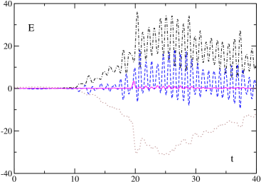
Figure 1: Energy conservation; parameters $m=\eta=\lambda=1$, $a=6$; dotted line: classical energy, Eq.(3.29); dash-dotted line: fluctuation energy, Eq.(3.30); dashed line: interaction energy, Eq.(3.31); solid line: self-interaction of the fluctuations, Eq.(3.32). The total energy (not displayed) is $E=(2.39\pm 0.001)\times 10^{-5}$.

6.2 Parametrization and parameter sets

The parameter space, encompassing $\eta,\lambda$ and $a$ is quite large, so before presenting numerical results we try to get some qualitative insight into the physics to be expected in certain ranges of their numerical values. The parameter $m$ sets the overall scales and is put equal to $m=1$.

While in Sec. 2, we introduced a scaling of the fields, (2.10), which was suitable for the canonical formalism on the basis of the Hamiltonian (2), the discussion of the results is more transparent if we introduce the $\alpha-\beta-$ parametrization widely used in bounce computations [4, 33, 34, 35]. One introduces the rescaling $X=mx$ and $\Phi=m^{2}\hat{\Phi}/2\eta$. Then for infinite space the classical action takes the form

$$S_{\rm cl}=\frac{m^{4}}{4\eta^{2}}\int d^{2}X\left[\frac{1}{2}\left(\nabla_{X}\hat{\Phi}\right)^{2}+\hat{U}(\hat{\Phi})\right]=\beta\hat{S}_{\rm cl}(\alpha)\;,$$ (6.2)

with $\beta=m^{4}/4\eta^{2}$, $\alpha=\lambda\beta/m^{2}$ and

$$\hat{U}(\hat{\Phi})=\frac{1}{2}\hat{\Phi}^{2}-\frac{1}{2}\hat{\Phi}^{3}+\frac{\alpha}{8}\hat{\Phi}^{4}\;.$$ (6.3)

While $\beta$ multiplies the classical action the one-loop effective action is a function of $\alpha$ only. So for large $\beta$ the system essentially becomes classical and the quantum effects only lead to small corrections while for small $\beta$ the quantum effects become large. The parameter $\alpha$ determines the shape of the potential: for $\alpha\to 1$ we get a symmetric double-well potential, for small $\alpha$ the right hand well becomes much deeper than the left hand one, the barrier between the wells becomes shallow. For bubble nucleation $\alpha\to 1$ is the thin-wall limit, where the bubble size becomes very large.The case $\alpha>1$ is of no interest here, as the minimum at $\Phi=0$ then becomes the global minimum.

We will in the following consider parameter sets with fixed $\alpha$ and $\beta$, i.e., fixed $\lambda$ and $\eta$, and study the dependence on $a$.

For finite space extension the semiclassical tunneling action of a spatially homogeneous bounce is given by

$$S_{\rm bounce}=2\pi a\beta\int_{0}^{\hat{\Phi}_{0}}d\hat{\Phi}\sqrt{\hat{U}(\hat{\Phi})}\;,$$ (6.4)

where

$$\hat{\Phi}_{0}=\frac{2}{\alpha}\left(1-\sqrt{1-\alpha}\right)$$ (6.5)

is the zero at the right hand side of the potential barrier. For fixed $\alpha,\beta$ the tunneling via a homogeneous bounce should shut off with increasing $a$. The tunneling will then occur via local bounces, as considered recently in the Hartree approximation in [36, 37].

The transition rate obtained from the homogeneous bounce, Eq. (6.4), will only have a qualitative relation to the observed tunneling phenomena which will be characterized by the occurrence of resonances. For quantum mechanical tunneling this was already observed in Ref.[20]. In order to estimate the separation of the resonances we consider the approximate spectra of the left and right wells, treating them as separate oscillators. The resonances can then be thought of as arising from the degeneracy of levels in the left and in the right wells. From the Hamiltonian and the potential written in canonical variables, Eqs. (3.4) and (3.5), we see that the energies of the left hand oscillator are $E_{n}^{l}=(n+1/2)m$. The right hand oscillator potential has its minimum at

$$\chi_{0}^{+}=\sqrt{2\pi a}\Phi_{+}=\sqrt{2\pi a}\frac{2\eta}{\lambda}\hat{\Phi}_{+}\;,$$ (6.6)

with

$$\hat{\Phi}_{+}=\frac{3}{2\alpha}\left(1+\sqrt{1-\frac{8}{9}\alpha}\right)\;,$$ (6.7)

and the energy levels are given by

$$E_{n}^{r}=\left(n+\frac{1}{2}\right)\omega_{+}+\tilde{U}(\chi_{0}^{+})\;.$$ (6.8)

Here

$$\omega_{+}^{2}=\tilde{U}^{\prime\prime}(\chi_{0}^{+})=2m^{2}\left[\frac{9}{8\alpha}\left(1+\sqrt{1-\frac{8}{9}\alpha}\right)-1\right]$$ (6.9)

and

$$\tilde{U}(\chi_{0}^{+})=2\pi a\beta\hat{U}(\hat{\Phi}_{+})<0\;.$$ (6.10)

So the condition for a degeneracy of a level in the spectrum of the right hand well with the ground state of the left hand well (our initial state) is

$$2\pi aU(\Phi_{+})+\left(n+\frac{1}{2}\right)\omega_{+}=\frac{1}{2}m\;.$$ (6.11)

We present here the dependence of the tunneling phenomena on the spatial length scale $a$. If the degeneracy holds for some value $a$ and an integer $n$, it will hold again for $a^{\prime}=a+\Delta a$, $n^{\prime}=n-\Delta n$ with

$$\Delta a=-\frac{\omega_{+}}{2\pi U(\Phi_{+})}\Delta n\;.$$ (6.12)

The constant multiplying $\Delta n$ on the right hand side determines the spacing of resonance levels as a function of $a$ at fixed $\alpha$ and $\beta$. Of course we may also have resonances between excited states of the left well and those of the right hand well, but, as our initial state will roughly correspond to the ground state of the left hand well, these will be less important. Another, more essential feature is the excitation of field quanta of the nonzero modes. These will have a dissipative effect on the dynamics of the zero mode and broaden the resonances. The interaction consists in a deformation of the potential in which the zero mode is moving, which takes the form

$$U_{0}(\chi_{0},t)=\tilde{U}(\chi_{0})+(\tilde{U}^{\prime\prime}(\chi_{0})-m^{2}){\cal F}(t)\;.$$ (6.13)

If ${\cal F}(t)$ is negligible the evolution of the system proceeds like in the quantum mechanics of the zero mode. If ${\cal F}(t)$ remains small this time-dependent modulation of the potential will allow a few other approximate eigenstates of the zero mode to mix in, the resonant oscillations develop “higher harmonics” and become irregular. If ${\cal F}(t)$ gets large then the potential can be deformed in such a way that the potential barrier disappears entirely, in such cases the zero mode may “slide” into the new minimum. This happens if ${\cal F}(t)$ is positive; if ${\cal F}(t)$ is negative the potential is tilted counterclockwise and the barrier is enhanced.

6.3 Results of the numerical simulations

We have performed a study of tunneling as a function of the radius of the space manifold $S_{1}$, for fixed values of the parameters $\alpha$ and $\beta$, or $\lambda$ and $\eta$; the mass is chosen to be unity, which determines length and time scales. We have considered four parameter sets: set $I$: $\alpha=0.8,\beta=0.5$, i.e., $\lambda=1.6,\eta=1/\sqrt{2}$; set $II$: $\alpha=0.6,\beta=2$, i.e., $\lambda=0.3,\eta=1/\sqrt{8}$; set $III$: $\alpha=0.4,\beta=1$, i.e., $\lambda=0.4,\eta=1/2$; set $IV$: $\alpha=0.25,\beta=0.25$, i.e., $\lambda=\eta=1$. For set $II$ we expect the quantum corrections to be small, for sets $I$ and $IV$ we expect large quantum corrections, and moderate ones for set $III$.

We have studied in general the behavior of the average of the zero mode $<\chi_{0}(t)>$, of the fluctuations (fluctuation integrals, particle number, and the various energies), and of the wave function $\psi_{0}(\chi_{0})$ of the zero mode, as functions of time. As the main indicator of the general behavior we use the maximal value attained by the expectation value of the zero mode during the time evolution. We denote this value as $\bar{\varphi}_{0}$. In those cases where we have effective tunneling, this zero mode average settles at a value of $\varphi_{0}$ beyond the potential barrier, the late time average being typically $20\%$ smaller than the maximal value.

We display in Figs. 1 to 4 the dependence of the maximal values $\bar{\varphi}_{0}$ of $<\varphi_{0}(t)>$, as functions of $a$ for the four parameter sets. The horizontal lines labelled by $\Phi_{m}$ and $\Phi_{0}$ indicate the position of the maximum of $U(\Phi)$ and the zero of the position between the two minima (the “end of the tunnel”). We see in all cases that an effective tunneling occurs as a resonance phenomenon. According to our estimate in the previous subsection, Eq. (6.12), the spacing of different resonances as a function of $a$ would be given by $\Delta a=0.529$ for set $I$, $\Delta a=0.0338$ for set $II$, $\Delta a=0.0167$ for set $III$ and $\Delta a=0.0166$ for set $IV$. The observed spacings roughly correspond to these estimates. We note that also the excited states of the left hand oscillator or of the nonzero modes can come into play, so if we observe some irregular spacings this may be due to such effects. When compared to similar figures obtained in quantum mechanical simulations [20] the resonances seen in our simulations are broader. We observe that even on resonance the maximal value of $<\varphi_{0}>$ never reaches the second minimum (the “true vacuum”). In part this is due to the fact that the effective potential seen by the zero mode is modified by the quantum fluctuations, moreover, even at late times the wave function generally retains a finite probability density near the false vacuum $\varphi_{0}=0$. This will be discussed in more detail below.

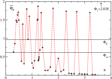
Figure 2: The maximum $\bar{\varphi}_{0}$ of the expectation value $<\varphi_{0}(t)>$ for set $I$, $\alpha=0.8,\beta=0.5$, as a function of $a$.

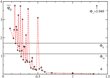
Figure 3: The maximum $\bar{\varphi}_{0}$ of the expectation value $<\varphi_{0}(t)>$ for set $II$, $\alpha=0.6,\beta=2$, as a function of $a$.

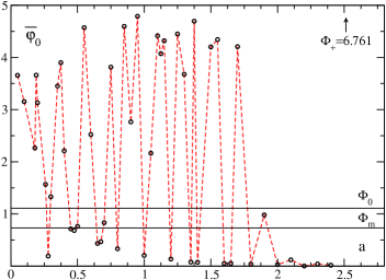
Figure 4: The maximum $\bar{\varphi}_{0}$ of the expectation value $<\varphi_{0}(t)>$ for set $III$,$\alpha=0.4,\beta=1$, as a function of $a$.

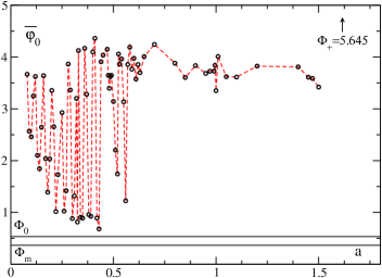
Figure 5: The maximum $\bar{\varphi}_{0}$ of the expectation value $<\varphi_{0}(t)>$ for set $IV$,$\alpha=0.25,\beta=0.25$, as a function of $a$.

For the parameter sets $I-III$ the tunneling shuts off entirely at higher values of $a$ as expected from the bounce action (6.4) being proportional to $a$. As large $\beta$ implies a large classical action and, therefore, a small semiclassical tunneling rate, this shutting-off already happens at small values, $a\simeq 0.5$, for set $II$. For set $I$ on still finds resonant tunneling for $a>3$. However, the transition time at the resonances increases substantially ($t\simeq 1000$ at the last peak in Fig. 1), between the resonances the amplitude of the zero mode oscillations decays exponentially with $a$, as for sets $II$ and $III$, and the zero mode wave function displays no tunneling at all. The case of set $IV$ is quite different. Here at large $a$ the system always tunnels. This effect is due to the fact that the quantum fluctuations deform the potential seen by the zero mode, Eq. (6.13) into a potential without barrier, the late time wave function extending over a range from $-5$ to $+20$, we call this kind of transition a sliding transition. We will discuss this below.

The results for the maximal value $\bar{\varphi}_{0}$ of the zero mode average display a global picture of the tunneling in the asymmetric double well potential in quantum field theory. They look quite different from what one usually assumes to happen in “false vacuum decay”, when one just considers the homogeneous bounce action (6.4) without or with quantum corrections. We will now discuss in some more detail the evolution of the zero mode wave function.

For all parameter sets and all values of $a$ the wave function of the zero mode initially evolves slowly; it becomes slightly asymmetric and develops a tail into the region of the potential barrier. Here already the fact that we do not restrict it to be Gaussian is of prime importance. The further behavior then depends on the parameter sets.

On the resonances the wave function, which initially is essentially the ground state wave function of the left well first connects to a particular wave function in the right well, obviously the one of the degenerate level. This is seen in Fig. 6 , the well-defined number of peaks within the right hand well indicate a specific approximate level within the right hand well. If the fluctuations of the quantum field, i.e., the amplitudes of the $\varphi_{n}$, remain small, then one observes an oscillation forth and back between these two wave functions, as expected in a purely quantum mechanical system. If the nonzero field modes get excited, then these oscillations of the zero mode are disturbed, other wave functions mix in, as seen by the increasing number of peaks, in some cases the wave function looks quite chaotic.

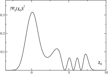
Figure 6: Probability density $|\psi_{0}(\chi_{0})|^{2}$ at intermediate times, here $t=10$, for $\alpha=0.8$, $\beta=0.5$, and $a=1.35$

Off resonance the expectation value of $\varphi_{0}$ oscillates regularly with a small amplitude. It still develops a tail into the right hand well, but this part of the wave functions remains small.

Beyond the resonance region there is efficient tunneling if the fluctuations of the nonzero momentum modes are large. In this case, while the wave function penetrates into the barrier region, the fluctuation integral becomes positive, the barrier disappears and the wave function slides down the hill retaining almost its initial Gaussian form.

The simulations of set II, $\alpha=0.6,\beta=2$ are expected to resemble most closely the case of quantum mechanics. The nonzero momentum quantum fluctations indeed remain small and we have the resonances expected from the qualitative picture of degenerate levels of the individual wells. The results for the expectation value of the zero mode and for the evolution of the wave functions correspond to these expectations. We present the regular oscillations of the zero mode on the resonance at $a=0.5$ in Fig. 7. We plot, in the same figure, the particle number ${\cal N}$ defined below Eq. (3.36), multiplied by $1000$. The wave function, shown at four different times in Fig. 8, is seen to return to itself almost exactly after half a period of $t\simeq 55$.

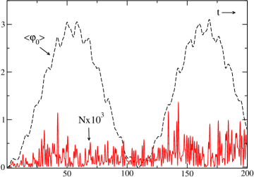
Figure 7: Evolution of the expectation value of the zero mode $<\varphi_{0}>$ and of the particle number $\cal N$; parameters $\alpha=0.6$, $\beta=2$, $a=0.5$.

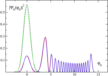
Figure 8: The zero mode wave function for $\alpha=0.6$, $\beta=2$, $a=0.5$; dashed lines: the wave functions at $t=0$ and $109$; solid lines: the wave functions at $t=50$ and $t=168$.

Set III is intermediate in the sense that with $\beta=1$ we expect the fluctuations of the nonzero modes to be sizeable but not really large. We find that tunneling is again characterized by the occurrence of resonances, and again shuts off at larger values of $a$, here around $a=2$. Around this value the resonant transitions occur on longer and longer time scales. So for $a>2$ we cannot exclude further resonances if we run the simulations for times longer than $t\simeq 300$.

For set IV the zero mode shows resonant behaviour at small $a$, but for $a>0.5$ the system always ends up in the right well. The actual evolution is quite involve here. Once the fluctuations set in, they tilt the potential in such a way that the barrier disappears and that the wave function can start to move right. Then the fluctuation integral ${\cal F}$ gets small again or negative, so the potential barrier appears again. This process repeats itself in an oscillatory way, and the wave function gradually shifts towards the deeper well. This is displayed in Fig. 9. At late times the quantum modes still oscillate with a sizeable amplitude, so that the potential seen by the zero mode keeps on changing and can neither be considered to be double or single well. A typical wave function at late times is shown in Fig. 10 for $a=1.2$ and $t=30$. One sees no trace of a double-well structure. In spite of the complexity of the wave function the energy is still conserved better than one part in $10^{8}$ (see Fig. 1).

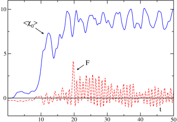
Figure 9: Evolution of the expectation value $<\varphi_{0}(t)>$ and of the fluctuation integral ${\cal F}(t)$ for $\alpha=\beta=0.25$ (set IV) and $a=1.2$.

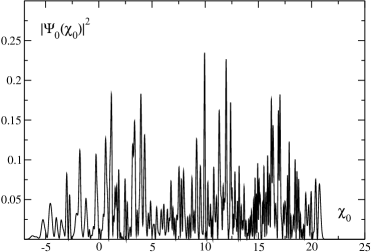
Figure 10: The wave function after tunneling, $\alpha=\beta=0.25$ (set IV) and $a=1.2$ and time $t=30$.

The situation becomes more transparent for larger values of $a$ . We show results for $a=6$. Here again the potential is tilted by the fluctuations, but the fluctuation integral remains positive on the average at late times. This implies that the barrier has disappeared definitively. The transition can be described as a sliding of the wave function towards the new minimum. This is displayed in Fig. 11.

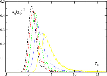
Figure 11: Evolution of the wave function during the barrier transition: parameters $m=\eta=\lambda=1$; $a=6$; long-dashed line: $t=7$; dash-dotted line: $t=7.4$; short-dashed line: $t=7.8$; dotted line: $t=8.2$; straight line: $t=8.6$.

For the case under consideration, set $IV$ with $\alpha=0.25$ the potential is very asymmetric. So one may infer that the tilting of the potential is most effective here, and that this effect may in fact be limited to small values of $\alpha$. We therefore have performed simulations for $\alpha=0.8$ and $\beta=0.2$, i.e., for a more symmetric potential, but again with large quantum corrections. We find that for values of $a>1$ the transition again occurs by sliding, but that at late times the fluctuation integral becomes negative and the potential is tilted in such a way that the barrier reappears. This is presented in Figs. 12 and 13. The wave function at late times is then found to have sizeable amplitudes in both wells.

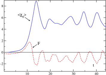
Figure 12: Evolution of the expectation value $<\varphi_{0}(t)>$ and of the fluctuation integral for $\alpha=0.8$, $\beta=0.2$, and $a=5$.

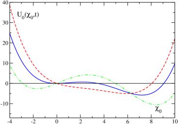
Figure 13: Evolution of the effective potential $U_{0}(\chi_{0},t)$; solid line: $t=0$; dashed line: $t=11$; dash-doubledotted line: $t=13$.

So it seems that sliding occurs universally for small $\beta$ and large $a$.

7 Conclusions and outlook

We have presented here an analysis of global tunneling in quantum field theory on a compact space. This analysis was based on a real-time formulation, using the time-dependent Hartree approximation. We have performed numerical simulations of a system where the wave function of the zero momentum mode evolves as a solution of the Schrödinger equation, while the nonzero momentum modes are treated in the Gaussian approximation. The approximation includes the back-reaction of the nonzero momentum modes onto the zero momentum mode and onto themselves. The renormalized equations were obtained using the 2PPI formalism, adopted here to a system with finite space extension.

We have found that tunneling for such systems occurs in a variety of different ways. For large $\beta$, implying small field fluctations, the system behaves like a quantum mechanical system with a single degree of freedom. Tunneling is effective whenever it connects degenerate modes, so varying the parameters, here the radius $a$, one finds resonance enhancements. For large spatial extension $a$ this resonant tunneling shuts off as expected from the fact that the WKB integral over the barrier is proportional to $a$. For smaller values of $\beta$ the nonzero momentum modes, the modes which make up the quantum field, are enhanced and modify the quantum mechanical behavior. If this enhancement is weak it can be considered as a kind of dissipation; the mean value of the zero mode shows regular periodic oscillations, on and off resonance. On resonance this again involves two or a few more modes in the two separate wells, off resonance the wave function essentially remains in the left well, with some tail in the right hand well. For parameter sets where the excitation of the nonzero momentum modes becomes sizeable, these regular oscillations are disturbed, the oscillations of the mean value of the zero mode become irregular and so do the wave functions of the zero mode. Off resonance at late times the system again remains concentrated in the left hand well. On resonance at late times the wave function extends over the entire region allowed at the given energy. While the system may then be considered as having tunneled, it certainly ends up in a rather complex excited state.

If the quantum corrections are large the system exhibits another phenomenon: the quantum fluctuations tilt the effective potential for the zero mode in such a way that the barrier disappears entirely. In such cases the system wave function can be observed to slide into the new minimum. The disappearance ot the barrier may be a temporary effect. It is due to the substantial quantum excitations once the wave function enters the barrier, leading to negative squared masses for the fluctations. At late times the potential may become be a double-well potential again, or the barrier may disappear defintively.

This variety of phenomena observed here in a real-time analysis cannot be expected to be described by a simple transition rate formula. A better approximation than the classical bounce action, Eq. (6.4), could be obtained by fitting together WKB patches within the allowed and forbidden regions or by applying a time-dependent WKB approximation to the $k=0$ mode itself, as done for quantum mechanics in Ref. [27]. However, the advantage of dealing with analytic or semi-analytic formulas is lost at the latest if one includes the nonzero momentum fluctuations. In most cases they cannot be evaluated analytically and, as implied by the present analysis, they cannot be expected to give reliable estimates. For homogeneous tunneling they exhibit the phenomenon of multiple unstable modes: if the unstable mode for $k=0$ has the squared frequency $-|\omega_{-}|^{2}<0$ then the $k\neq 0$ modes will have an eigenmode with the eigenvalue $k^{2}/a^{2}-|\omega_{-}|^{2}$ which is positive for small $a$ but will become negative whenever $a>a_{k}=k/|\omega_{-}|$. The interpretation of these modes is unclear, there is no trace of them in the numerical simulations.

With increasing $a$ one expects the system to become unstable with respect to inhomogeneous, local bounces. This instability may be closely related to the sliding phenomenon for which a strong excitation of $k\neq 0$ modes is crucial: the $k\neq 0$ modes are of course spatially inhomogeneous; if they are excited substantially they may be interpreted as classical fluctuations. For $k=n$ they have the general form of a chain of $n$ bubbles, much in the way as they are depicted in Refs. [3, 4] for the decay of the false vacuum at finite temperature. It could be interesting to investigate this relation between inhomogeneous and homogeneous tunneling in a more quantitative way. Clearly, in view of this instability with respect to local bounces, our present analysis becomes unreliable at values $a>>1$.

The restriction to one compact space dimension was done in order to reduce technical complications to a minimum. Similar phenomena are expected for compact three-dimensional spaces. The discrete spectrum of momenta then becomes a discrete spectrum of angular momenta, whose excitation will be small for small $a$ and become more effective with increasing $a$. The potential seen by the homogeneous mode is again a double-well potential, so again resonances are expected to dominate the low $a$ regime. If gravity is included, like for transitions in de Sitter space, renormalization becomes problematic, especially if quantum backreaction is included. Still it would be interesting to investigate along these lines the relation between homogeneous transitions like the Hawking-Moss instanton and inhomogeneous ones like the Coleman-deLuccia bounce.

Of course it would be even more interesting to follow, in real time, the local creation of real vacuum bubbles including the associated excitation of quantum modes with back-reaction. This seems to be out of scope with the presently available numerical methods and computer facilities. Our calculations may elucidate in a qualitative way effects that are missed in the WKB approach to local transitions, even when quantum corrections are taken into account [34, 35, 36, 37].

References

- [1] S. R. Coleman, Phys. Rev. D15, 2929 (1977).
- [2] S. R. Coleman and F. De Luccia, Phys. Rev. D21, 3305 (1980).
- [3] A. D. Linde, Phys. Lett. B100, 37 (1981).
- [4] A. D. Linde, Nucl. Phys. B216, 421 (1983).
- [5] S. W. Hawking and I. G. Moss, Phys. Lett. B110, 35 (1982).
- [6] S. W. Hawking and N. Turok, Phys. Lett. B425, 25 (1998), [hep-th/9802030].
- [7] A. D. Linde, Phys. Lett. B129, 177 (1983).
- [8] K. Hirota, Phys. Rev. D61, 123502 (2000).
- [9] J. B. Hartle and S. W. Hawking, Phys. Rev. D28, 2960 (1983).
- [10] T. Vachaspati and A. Vilenkin, Phys. Rev. D37, 898 (1988).
- [11] A. Vilenkin, Phys. Rev. D50, 2581 (1994), [gr-qc/9403010].
- [12] A. Vilenkin, Nucl. Phys. Proc. Suppl. 88, 67 (2000), [gr-qc/9911087].
- [13] J.-y. Hong, A. Vilenkin and S. Winitzki, Phys. Rev. D68, 023520 (2003), [gr-qc/0210034].
- [14] D. H. Coule and J. Martin, Phys. Rev. D61, 063501 (2000), [gr-qc/9905056].
- [15] M. Bouhmadi-Lopez, L. J. Garay and P. F. Gonzalez-Diaz, Phys. Rev. D66, 083504 (2002), [gr-qc/0204072].
- [16] S. P. Kim, J. Korean Phys. Soc. 45, S172 (2004), [gr-qc/0403015].
- [17] V. A. Rubakov, Nucl. Phys. B245, 481 (1984).
- [18] D. Levkov, C. Rebbi and V. A. Rubakov, Phys. Rev. D66, 083516 (2002), [gr-qc/0206028].
- [19] J. Hong, A. Vilenkin and S. Winitzki, Phys. Rev. D68, 023521 (2003).
- [20] M. M. Nieto, V. P. Gutschick, F. Cooper, D. Strottman and C. M. Bender, Phys. Lett. B163, 336 (1985).
- [21] O. J. P. Eboli, R. Jackiw and S.-Y. Pi, Phys. Rev. D37, 3557 (1988).
- [22] F. Cooper, S. Habib, Y. Kluger and E. Mottola, Phys. Rev. D55, 6471 (1997), [hep-ph/9610345].
- [23] D. Boyanovsky, H. J. de Vega, R. Holman and J. F. J. Salgado, Phys. Rev. D54, 7570 (1996), [hep-ph/9608205].
- [24] J. Baacke, K. Heitmann and C. Patzold, Phys. Rev. D55, 2320 (1997), [hep-th/9608006].
- [25] S. A. Ramsey and B. L. Hu, Phys. Rev. D56, 678 (1997), [hep-ph/9706207].
- [26] R. Jackiw and A. Kerman, Phys. Lett. A71, 158 (1979).
- [27] F. Cooper, S.-Y. Pi and P. N. Stancioff, Phys. Rev. D34, 3831 (1986).
- [28] C. Destri and E. Manfredini, Phys. Rev. D62, 025008 (2000), [hep-ph/0001178].
- [29] P. Dirac, Proc. Camb. Phil. Soc. 26 (1930).
- [30] G. H. Hardy, Divergent series (Oxford University Press, Oxford, 1949), section 13.14.
- [31] J. Baacke and S. Michalski, Phys. Rev. D65, 065019 (2002), [hep-ph/0109137].
- [32] Y. Nemoto, K. Naito and M. Oka, Eur. Phys. J. A9, 245 (2000), [hep-ph/9911431].
- [33] M. Dine, R. G. Leigh, P. Y. Huet, A. D. Linde and D. A. Linde, Phys. Rev. D46, 550 (1992), [hep-ph/9203203].
- [34] J. Baacke and V. G. Kiselev, Phys. Rev. D48, 5648 (1993), [hep-ph/9308273].
- [35] J. Baacke and G. Lavrelashvili, Phys. Rev. D69, 025009 (2004), [hep-th/0307202].
- [36] Y. Bergner and L. M. A. Bettencourt, Phys. Rev. D69, 045012 (2004), [hep-ph/0308107].
- [37] J. Baacke and N. Kevlishvili, Phys. Rev. D71, 025008 (2005), [hep-th/0411162].