On the evolution of cosmic-superstring networks

Abstract

We model the behaviour of a network of interacting $(p,q)$ strings from IIB string theory by considering a field theory containing multiple species of string, allowing us to study the effect of non-intercommuting events due to two different species crossing each other. This then has the potential for a string dominated Universe with the network becoming so tangled that it freezes. We give numerical evidence, explained by a one-scale model, that such freezing does not take place, with the network reaching a scaling limit where its density relative to the background increases with $N$, the number of string types.

I Introduction

Despite the remarkable success of inflation inflation ; review in describing the observed patterns of the microwave anisotropy wmap there remains an active interest in cosmic strings as a serious player in the early universe Kibble:2004hq . Whilst it is now clear that cosmic strings cannot play a dominant role in structure formation their appearance in many scenarios, whether they be motivated by M-theory or supergravity leads us to consider them as a sub-dominant partner Contaldi:1998qs ; Jeannerot:2003qv ; Wyman:2005tu with tensions of the order $G\mu\leq 10^{-6}$. Depending on the model and the allowed decay processes for the string network, the bounds on $G\mu$ can be significantly strengthened. These could include the production of dilatons Babichev:2005qd , of gravitational waves Damour:1996pv or even the possibility of loops of string being trapped in the compact dimensions leading to a monopole type problem for the strings Avgoustidis:2005vm .

For many years the main connection between cosmic strings and superstrings was that both were much studied but never observed. Indeed, the high tension of fundamental strings, placed at around the Planck scale, ruled then out as cosmic string candidates. However, over the past decade or so, more interesting solutions have begun to emerge in string theory, involving warped compactifications or large extra dimensions. One of the by-products has been a realization that these warp factors play a crucial role in determining energy scales of compactifications Randall:1999ee . In string theory these warp factors are sourced by brane-fluxes and much has been made of their use in model buildingGiddings:2001yu ; Kachru:2003aw .

Recently the possibility that the same basic mechanism could provide both the inflaton and lead to the formation of cosmic strings has received renewed attention in the context of braneworlds bab ; tye ; Kachru:2003sx ; DKVP ; DVnew ; Copeland:2003bj . Some consistency conditions for superstrings to act as cosmic strings were given in Copeland:2003bj , in particular the KKLMMTKachru:2003sx picture of IIB string theory has a warp factor which allows the Dirichlet-fundamental strings $(p,q)$ bound state to have reduced tensions and behave as cosmic strings. Such cosmic strings are different to the standard Abelian strings as they offer more ways of interacting; two different $(p,q)$ strings could pass though each other, or they could reconnect in one of the two ways depicted in Fig. 1Jackson:2004zg . A network formed from such strings will therefore have quite different properties. Networks formed from Abelian strings consist of loops and long strings, $(p,q)$ networks also contain loops and long string, but there are also links which start and end at a three-point vertex Fig. 1. The presence of these links in non-Abelian string networks has lead authors to speculate the possible existence of a frozen network which comes to dominate the matter content of the Universebpsnet ; Spergel:1996ai ; Bucher:1998mh . A number of authors have begun to reconsider the evolution of the more complicated dynamics associated with cosmic superstrings, and argued in general that scaling solutions are achievedmaria ; martins ; shellard . For example, recently there has been work suggesting that such networks of $(p,q)$ strings reach a scaling behaviour, where the density of strings scales with that of the background energy density of the Universe Tye:2005fn . Here we re-consider the field theory model of Spergel:1996ai , which can be thought of as containing $N$ basic strings and $\frac{1}{2}N(N-3)$ bound states to give a total of $\frac{1}{2}N(N-1)$ different species of string. We shall see from the numerical simulations that as $N$ increases, so does the scaling density. This is to be expected because the network loses string via the formation of loops, and loops can only form from the reconnection event caused by two strings of the same type intersecting. Because the chance of a string meeting the same type decreases for large $N$ then the probability of loop formation at reconnection goes down. Although we do not claim this model accurately describes a network of $(p,q)$ strings it does have the important property that strings reconnect as they pass through each other, so creating the links which are the main difference to the standard cosmic string scenario. An important difference between our model and that of the $(p,q)$ relates to the allowed string tension. While our field theory gives all strings the same tension, the tension of a $(p,q)$ string increases for larger $p$, $q$ having the effect that low $p$, $q$ will be preferred dynamically. From the perspective of the field theory model this would correspond to having $N$ small.

Before discussing the dynamics associated with a network of non-abelian strings, we first remind the reader about some of the basic properties associated with ordinary abelian strings. For a comprehensive review see vilenkin:1994 .

The initial distribution of a network of strings is comprised of a combination of infinite strings that stretch across the universe and a scale invariant distribution of loops of string. Roughly 80% of the string is initially infinite in length and 20% is in loops. There exist a series of characteristic length scales on the network, but the one we are interested here is $\xi$, which corresponds to the typical separation between strings, and is given in terms of the volume $V$ and total length $L$ of strings by $\xi^{2}=V/L$. Other possible scales correspond to the typical curvature scale on the strings, and the small scale structure on the string network. As the universe expands, the network evolves and the characteristic length scales change with time as well. There are a number of physical processes that occur allowing the network to lose energy. The long strings can cross themselves forming loops which are chopped off the long strings, strings oscillate and because they are so massive they radiate energy through gravitational radiation. For our case, where we are considering a field theory model, the prominent decay mode will be through particle production. Meanwhile the long strings are stretched by the expansion, which increases the energy stored in the network. Hence there are competing effects which act against each other. Determining precisely how such a network evolves is a challenge that has proved difficult to solve exactly. The equations of motion are non-linear and the requirement of keeping track of the whole network in case new loops are formed from string intersections, requires considerable computing power. The net result is that the correlation length $\xi$ scales with the Hubble radius, leading to the ratio of the string energy density and the background radiation/matter energy density becoming a constant, implying that the strings provide a fixed contribution to the total energy density in the universe. This scaling solution formed the backbone of investigations into string dynamics. The initial loop distribution is modified to one where the number density of loops of size $l$ falls off as a power law in both the radiation and matter dominated eras, whilst maintaining the scale invariant distribution. The case for non-abelian strings is not as well understood, not least because much less effort has gone into following the evolution of these more complicated objects. Aryal et al Aryal:1986cp investigated the formation of $Z_{3}$ strings. Based on numerical simulations they argued that unlike the case for Abelian strings, the initial loop distribution was not a scale invariant power law distribution but rather it was better approximated by an exponential distribution with the number density falling off exponentially with loop length. The majority of the string length is initially to be found in one network taking up 93% of the total string length, with the rest in loops and much smaller networks. It raised the important question, what happens to such a non-abelian network, and this was partly addressed in Refs.  Vachaspati:1986cc ; Spergel:1996ai ; McG ? In this paper we will look more closely at the evolution of non-abelan strings, and show that they always appear to enter a scaling regime with a corresponding loop distribution that, rather than having a scale invariant power-law distribution, instead appears to be exponential. We will follow and modify the approach developed by Vachaspati and Vilenkin in Ref. Vachaspati:1986cc where the authors investigated the evolution of a network of strings connected to monopoles.

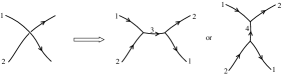
Figure 1: Example of formation of string segments due to non-intercommuting .

II one scale model

In this section we shall describe an analytic approach to understanding the scaling regime of a network of non-Abelian string. In what follows we will assume that the network evolution is described by a single length-scale, $\xi$, and shall see that the solution to this model is that a network evolves in a self-similar fashion with $\xi\sim t$, just as for Abelian networks. We start by writing down the evolution equation for a network containing a single string species evolving in an expanding background with Hubble parameter $H=\dot{a}/a$, where $a$ is the scale factor and $\dot{a}\equiv\frac{da}{dt}$. Taking the pressure of the string network as $p=\gamma\rho$, where $\rho$ is the energy density of the strings, and $\gamma$ is the equation of state parameter, then the fluid equation is

$$\dot{\rho}=-3H(1+\gamma)\rho-c_{p}\rho/\xi.$$ (2.1)

The first term on the right hand side includes the work done by the system per unit volume per unit time, and the second term describes the process of energy loss from strings by particle emission Vincent:1997cx . Taking $\mu$ to be the string tension we define the network length-scale $\xi$ through the string density,

$$\rho\sim{\mu\xi\over\xi^{3}}.$$ (2.2)

For a scale factor $a\propto t^{\nu}$, then

$$\dot{\xi} = \frac{3}{2}(1+\gamma)\nu\xi/t+\frac{c_{p}}{2}$$ (2.3)

$$= \kappa\xi/t+\lambda$$ (2.4)

where $\kappa=\frac{3}{2}(1+\gamma)\nu$, $\lambda=\frac{c_{p}}{2}$. This can be solved to give Vachaspati:1986cc

$$\xi(t) = \frac{\lambda}{1-\kappa}t+Kt^{\kappa}.$$ (2.5)

Causal evolution of the network requires $\xi$ to grow no faster than $t$ so we must have $\kappa\leq 1$, leading to $\xi\propto t$ asymptotically, typical of self-similar evolution.

Now we include loop production and reconnection. Following Vachaspati:1986cc , normally we would expect that most of the loops chopped off the network are likely to be recaptured, both events occurring on a time-scale of order $\xi(t)$. However, including expansion, the two events are not quite equal. In a time interval $\xi$, the density of strings is reduced by a fraction $\xi/t$, leading to a similar reduction in the probability of loop absorption. In other words there is an imbalance with the infinite network losing energy to loops at the rate $\dot{\rho}_{\rm loops}\sim-(\xi/t)(\mu\xi/\xi^{4})$ or

$$\dot{\rho}_{\rm loops}\sim-c_{l}\rho/t,$$ (2.6)

where we expect the constant $c_{l}\sim 1$. Things change even more in our particular case. We shall see later that there is not one type of string but $\frac{1}{2}N(N-1)$, which can be thought of as bound states of $N$ types of underlying string. Now, imagine two of these strings $N_{1}$ and $N_{2}$ which cross one another. Only when $N_{1}$ and $N_{2}$ are the same will they form loops. Hence the probability of forming loops is decreased in our case by an additional factor of $2/(\frac{1}{2}N(N-1)+1)$. We see this by noting that for $n(=\frac{1}{2}N(N-1))$ string species there are $\frac{1}{2}n(n+1)$ distinct pairings of string, of which $n$ will pair up the same type. So the chance of a random pairing containing two of the same species is ${n\over\frac{1}{2}n(n+1)}={2\over\frac{1}{2}N(N-1)+1}$ In other words we have

$$\dot{\rho}_{\rm loops}\sim-{2c_{l}\over\frac{1}{2}N(N-1)+1}{\rho\over t}.$$ (2.7)

In the rate equation (2.1) we now have

$$\dot{\rho} = -3H(1+\gamma)\rho-c_{p}\rho/\xi+\dot{\rho}_{\rm loops}$$ (2.8)

$$= -2\kappa\rho/t-c_{p}\rho/\xi-{2c_{l}\over\frac{1}{2}N(N-1)+1}{\rho\over t}.$$ (2.9)

Note the form of the loop term is simply to re-normalise the work-done contribution. In other words the solution for the characteristic length scale is as we quoted earlier but with a new $\kappa$:

$$\xi(t)={\lambda\over 1-\kappa_{N}}t+K_{N}t^{\kappa_{N}}$$ (2.10)

where $\kappa_{N}=\kappa+\frac{c_{l}}{\frac{1}{2}N(N-1)+1}$. Now we have obtained the characteristic length of the network as a function of N we can compare this to our numerical solutions, which we now describe.

III numerical model

In order to model a network of strings which do not intercommute, but rather form links between the two string segments as they cross (see Fig. 1) we followed the techniques described in Spergel:1996ai for setting up a linear sigma model. This is an approximation for describing a scalar field in the long wavelength limit where the field is taken to live on its vacuum manifold. In order to have different types of string this manifold must have more than one non-contractible loop, with each such loop corresponding to a string solution. We take the vacuum as given in Spergel:1996ai , and depicted in Fig. 2, which takes the form of $N$ spokes whose ends are identified, noting that $N=2$ corresponds to the usual case of a single species of string footnote . In general there are $\frac{1}{2}N(N-1)$ species corresponding to the number of incontractible loops in the vacuum. For example, referring to Fig. 2 we could form strings from the loops AOBA, AOCA, BOCB,…

Figure 2: Vacuum manifold for the sigma model, the ends of the spokes are identified.

Therefore we evolve a scalar field which takes values in $[0,\pi)\times\hbox{\mybb Z}_{N}$ and has a canonical kinetic term. The initial conditions are chosen such that the field takes random values at each lattice site and we use a $300^{3}$ lattice. The first set of simulations were performed in Minkowski space and the results for the network length-scale are given in Fig. 3, showing how $\xi$ evolves in time for various $N$.

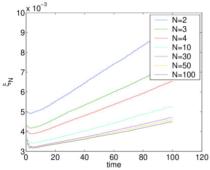
Figure 3: The evolution of the typical string length-scale as a function of N.

Note that the network approaches a scaling solution in each case, with $\xi\propto t$. Also, in the simulations with a larger number of species the network grows more slowly in time, as expected from (2.10), corresponding to a higher string density. The rate of increase of the network length-scale may now be extracted from the simulations by writing the late time behaviour of the simulation length-scale as $\xi_{sim}=\alpha t$, which can then compared to the asymptotic analytic form (2.10)

$$\xi(t)\rightarrow{\lambda\over 1-\kappa_{N}}t$$ (3.11)

In Fig. 4, we plot $\alpha$ as a function of $N$ for the simulations given in Fig. 3 with the analytic form shown on the graph for comparison. Although the match is by no means perfect it does illustrate the general behaviour that $\xi$ increases more slowly as the number of string species increases, and also that the gradient $\alpha$ asymptotes to a constant rather than zero, meaning that even for an arbitrarily large number of species the network will still scale rather than freeze. It is worth noting that our model underestimates the value of $\dot{\xi}_{N}$, corresponding to an overestimate of the scaling density. This means that the network has another mechanism by which it can lose energy. One possibility, identified by Tye:2005fn , is that the network will lose energy from the binding energy of two string species as they merge into a bound state, this could account for our overestimate of the scaling density.

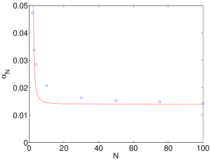
Figure 4: The slope of $\xi(t,N)$ as a function of N.

We have repeated the simulations for a radiation dominated Universe and present the results in Fig. 5. Plotted here is the ratio of the energy density in the string network to that of the background radiation as a function of time. For each value of $N$ there are two curves shown, each with a different initial value for the ratio of string density to radiation density. The figure shows that for a given $N$ each curve seems to approach the same constant value, indicating that there is a unique scaling solution for each $N$. Unfortunately the simulations run out of dynamic range before we are able to get accurate values for the scaling density, however we can see from the plots that the scaling density increases with $N$. As the density in radiation scales as $a^{-4}$, with $a\sim\sqrt{t}$ we have that the network density during scaling varies as $\rho_{s}\sim 1/\xi^{2}\sim 1/t^{2}$ which gives us the length-scale increasing as $\xi\sim\alpha t$ as before. Moreover, the simulations in the radiation background indicate that the scaling density increases with $N$ implying that $\alpha$ reduces as $N$ increases, consistent with our analytic approach.

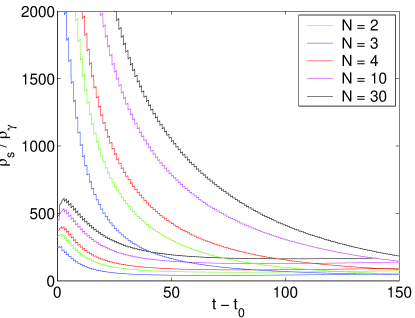
Figure 5: Scaling in radiation as a function of N.

We can provide further evidence for a scaling solution by measuring the total length of string contained in loops and the total length in links. In a scaling solution there should only be a single length-scale describing the properties of the network, as such we would expect the ratio of the amount of string in loops to the amount of string in links to approach a constant. To test this we focused on the case of $N=3$ and ran 100 simulations in order to minimize statistical errors. The results are plotted in Fig. 6 where we see how the ratio of loop length to link length evolves in time, we can clearly see that the ratio tends to a constant, furnishing us with further evidence that the network approaches scaling. We now proceed to describe the relative length distributions of the loops and links in these non Abelian networks.

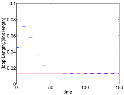
Figure 6: The ratio of loop length to link length for $N=3$.

IV length distribution

We have presented evidence that the string networks enter a scaling regime which can be described by a single length-scale. This however does not mean that all the loops and links have the same length given by $\xi$, so we now turn our attention to the distribution of the lengths in loops and links. It is well known that the more usual Abelian cosmic string has a power law distribution of loop length, $n(l){\rm d}l\sim l^{-5/2}{\rm d}l$ vilenkin:1994 , however our case for multiple species of string is more like the situation studied in Vachaspati:1986cc with three string species that could connect via heavy monopoles. There it was found that the distribution was more closely modelled by an exponential. Exponential distributions for string lengths were also found in Aryal:1986cp where the statistics of a random distribution of $\hbox{\mybb Z}_{3}$ strings were studied. Here, we have focused on the case $N=3$ and performed 100 simulations in order to get good statistics for the length distribution of loops and links. The results are given in Fig. 7, where we have plotted $\ln n(l)$ vs $l$, when the system has approached the scaling regime.

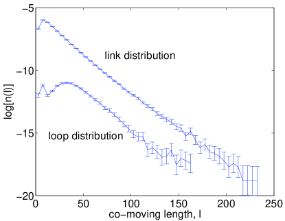
Figure 7: The distribution of loop/link lengths for $N=3$

At large $l$ the nearly-straight line of the plot clearly shows that the distributions are more accurately described by exponentials rather than power laws. We may model this by an exponential, dimensionless loop production function $f(l/\xi)$ by adapting the arguments found in vilenkin:1994 for the Abelian string. This function $f(l/\xi)$ describes the loss from the network of strings of length $l$. We consider the network to be in the scaling regime described by the length-scale $\xi$ such that (2.2) holds for the network. The loop production function $f(l/\xi)$ is defined such that $\mu f(l/\xi){\rm d}l/l$ is the energy lost in loops of length between $l$ and $l+{\rm d}l$ in volume $\xi^{3}$ per unit time. This then means that the loop density evolves according to

$$\dot{\rho}_{L} = -3H\rho_{L}+g\mu f(l/\xi)/\xi^{4},$$ (4.12)

where $g$ is a Lorentz factor to account for the loops created with non-zero centre of mass kinetic energy. We may rewrite this expression in terms of the dimensionless parameter $x=l/\xi$ and integrate to find

$$\rho_{L}(l,t)=\frac{g\mu l^{3\nu-3}}{\alpha^{3\nu+1}t^{3\nu}}\int_{l/\alpha t}^{\infty}{\rm d}x\;x^{2-3\nu}f(x).$$ (4.13)

Here we have taken $a(t)\sim t^{\nu}$, $\xi=\alpha t$, note that the radiation era corresponds to $\nu=\frac{1}{2}$. In order to get an exponential distribution of loop lengths we must therefore have a loop production function which contains an exponential, for example we may have

$$f(x)=bx^{p}\exp(-\beta x),$$ (4.14)

where $b,\,p$ and $\beta$ are constants. Taking this form and using $n(l,t)=\rho_{L}(l,t)/l$, (4.13) gives:

$$n(l,t) \simeq \frac{bg\mu l^{3\nu-4}}{\alpha^{3\nu+1}\beta^{3+p-3\nu}t^{3\nu}}\Gamma(3+p-3\nu,\beta l/\alpha t)$$ (4.15)

$$\rightarrow \frac{bg\mu}{\alpha^{3+p}\beta t^{2+p}}l^{p-2}\exp(-\beta l/\alpha t)$$

where in the final expression we have taken the limit $x>>1$. In principle we should be able to determine the dependence on $p$ from the numerical simulations, but this is not possible as it stands due to the statistical errors in the data at large loop length. In other words we can not yet determine the form of any power law correction to the pure exponential distribution.

We finally return to the distribution of the total string lengths in links and loops in the scaling regime, as shown in Fig. (6). We can understand the late time behaviour of this Figure based on our analytic approximations. If we consider the link length, $L_{\rm links}$ to be simply the difference between the total length of string $L$ and the length of string in loops, $L_{\rm loops}$, then we can write :

$${L_{\rm loops}\over L_{\rm links}}={1\over(\frac{L}{L_{\rm loops}}-1)}$$ (4.16)

Now in a large volume V, where the string tension is $\mu$ we know that

$${L\over L_{\rm loops}}={\rho\over\rho_{\rm loops}}$$ (4.17)

where $\rho_{\rm loops}$ is the energy density in loops defined from Eq. (4.13) by

$$\rho_{\rm loops}=\int_{t_{0}}^{\alpha t}\rho_{L}(l,t)dl$$ (4.18)

the limits of integration accounting for the largest loops excised at time $t$ and the smallest loops excised at time $t_{0}$. Performing the integral we find

$$\rho_{\rm loops}={bg\mu\over\alpha^{3}t^{2}}{1\over\beta^{3-3\nu+p}}F(\beta,p,t)$$ (4.19)

where

$$F(\beta,p,t)=\int_{\frac{t_{0}}{\alpha t}}^{1}x^{3(\nu-1)}\Gamma(3(\nu-1)+p,\beta x).$$ (4.20)

Now, $F$ is independent of $t$ at late times, hence we can extract the time dependence in Eq. (4.19) without knowing the full form of $F$. Now given $\rho=\frac{\mu}{\xi^{2}}$, and $\xi=\alpha t$, we find the late time behaviour in Eq. (4.17)

$${L\over L_{\rm loops}}={\alpha\beta^{3-3\nu+p}\over bgF}$$ (4.21)

which is independent of time, as required.

V conclusions

In this paper, in an attempt to model (p,q) strings arising out of compactifications of type IIB string theory, we have studied how a non-Abelian network of strings evolves. Such networks contain multiple vertices where many different types of string join together. For example, $Z_{3}$ strings have triple vertices where three different types of string join together. The result of these more complicated vertices is that non-Abelian networks have a richer variety of re-connections than their counterpart Abelian networks. Given this rich structure, from a cosmological point of view, we need to know whether such networks approach a scaling solution where they track the dominant background energy density or simply freeze, and stretch with the expansion of the universe leading to a string dominated Universe. By re-considering the field theory model of Spergel:1996ai , which can be thought of as containing $N$ basic strings and $\frac{1}{2}N(N-3)$ bound states to give a total of $\frac{1}{2}N(N-1)$ different species of string, we have shown both numerically and analytically that we always approach a scaling solution for all $N$, in other words the system does not freeze. All that happens is that as $N$ increases, so does the scaling density, asymptoting to a fixed value independent of $N$ for large $N$. Moreover, we have seen firm evidence that the associated distribution of loops and links is not governed by a power law as is the case for Abelain and $Z_{2}$ strings. Rather, as initially observed on smaller lattices by Aryal et al Aryal:1986cp and Vachaspati and Vilenkin Vachaspati:1986cc , the distribution drops off exponentially fast with loop size. We have attempted to explain this distribution based on our one-scale model, and argued why the loop-link ratio tends to a constant at late times for the case of $Z_{3}$ strings. There is much that remains to be done. Perhaps the most obvious thing is to allow the strings to have different tensions in this field theory model. In a very nice paper, Tye et al have been doing just that in the context of modelling cosmic superstrings Tye:2005fn . It would be worthwhile to see whether the field theory mimics their results or not. In particular once we have different tensions, it would be interesting to see how much string of each tension exists in a scaling network. One of the nice features about our approach is that we can produce the strings in an initial phase transiton and watch them evolve. It would be interesting to see how quickly the heavier tension strings appear, starting say from a network of light strings.

Acknowledgements The authors would like to thank PPARC for financial support, Nuno Antunes for collaboration in the early stages of the project and Mark Hindmarsh for useful discussions. P. M. S. would like to acknowledge extensive use of the UK National Cosmology Supercomputer funded by PPARC, HEFCE and Silicon Graphics.

References

-
(1)
A. H. Guth, Phys. Rev. D23 (1981) 347;
A.D. Linde, Phys. Lett. B108 (1982) 389;
A. Albrecht and P. J. Steinhardt, Phys. Rev. Lett. 48 (1982) 1220;
S. W. Hawking and I. G. Moss, Phys. Lett. B 110, 35 (1982). - (2) A. R. Liddle and D. H. Lyth, “Cosmological Inflation and Large-Scale Structure”, Cambridge University Press (2000)
-
(3)
C.L. Bennett et. al., Astrophy. J. Suppl. 148
(2003) 1,
[arXiv:astro-ph/0302207];
D. N. Spergel et al. [WMAP Collaboration], Astrophys. J. Suppl. 148, 175 (2003) [arXiv:astro-ph/0302209]. - (4) T. W. B. Kibble, [arXiv:astro-ph/0410073].
- (5) C. Contaldi, M. Hindmarsh and J. Magueijo, Phys. Rev. Lett. 82, 2034 (1999) [arXiv:astro-ph/9809053].
- (6) R. Jeannerot, J. Rocher and M. Sakellariadou, Phys. Rev. D 68, 103514 (2003) [arXiv:hep-ph/0308134].
- (7) M. Wyman, L. Pogosian and I. Wasserman, arXiv:astro-ph/0503364.
- (8) E. Babichev and M. Kachelriess, arXiv:hep-th/0502135;
-
(9)
T. Damour and A. Vilenkin,
Phys. Rev. Lett. 78, 2288 (1997)
[arXiv:gr-qc/9610005];
T. Damour and A. Vilenkin, Phys. Rev. D 71, 063510 (2005) [arXiv:hep-th/0410222]; - (10) A. Avgoustidis and E. P. S. Shellard, arXiv:hep-ph/0504049.
- (11) L. Randall and R. Sundrum, Phys. Rev. Lett. 83, 3370 (1999) [arXiv:hep-ph/9905221].
- (12) S. B. Giddings, S. Kachru and J. Polchinski, Phys. Rev. D 66, 106006 (2002) [arXiv:hep-th/0105097].
- (13) S. Kachru, R. Kallosh, A. Linde and S. P. Trivedi, Phys. Rev. D 68, 046005 (2003) [arXiv:hep-th/0301240].
-
(14)
G. R. Dvali and S. H. H. Tye,
Phys. Lett. B 450, 72 (1999)
[arXiv:hep-ph/9812483];
S. H. S. Alexander, Phys. Rev. D 65, 023507 (2002) [arXiv:hep-th/0105032];
C. P. Burgess, M. Majumdar, D. Nolte, F. Quevedo, G. Rajesh and R. J. Zhang, JHEP 0107, 047 (2001) [arXiv:hep-th/0105204];
G. R. Dvali, Q. Shafi and S. Solganik, arXiv:hep-th/0105203. -
(15)
N. Jones, H. Stoica and S. H. Tye,
JHEP 0207, 051 (2002)
[arXiv:hep-th/0203163];
S. Sarangi and S. H. Tye, Phys. Lett. B 536, 185 (2002) [arXiv:hep-th/0204074];
N. T. Jones, H. Stoica and S. H. H. Tye, Phys. Lett. B 563, 6 (2003) [arXiv:hep-th/0303269]. - (16) S. Kachru, R. Kallosh, A. Linde, J. Maldacena, L. McAllister and S. P. Trivedi, JCAP 0310, 013 (2003) [arXiv:hep-th/0308055].
- (17) G. Dvali, R. Kallosh and A. Van Proeyen, JHEP 0401, 035 (2004) [arXiv:hep-th/0312005].
- (18) G. Dvali and A. Vilenkin, JCAP 0403, 010 (2004) [arXiv:hep-th/0312007].
- (19) E. J. Copeland, R. C. Myers and J. Polchinski, JHEP 0406, 013 (2004) [arXiv:hep-th/0312067].
- (20) M. G. Jackson, N. T. Jones and J. Polchinski, arXiv:hep-th/0405229.
- (21) A. Sen, JHEP 9803, 005 (1998) [arXiv:hep-th/9711130].
- (22) D. Spergel and U. L. Pen, Astrophys. J. 491, L67 (1997) [arXiv:astro-ph/9611198].
- (23) M. Bucher and D. N. Spergel, Phys. Rev. D 60, 043505 (1999) [arXiv:astro-ph/9812022].
- (24) M. Sakellariadou, arXiv:hep-th/0410234.
- (25) C. J. A. Martins, Phys. Rev. D 70, 107302 (2004) [arXiv:hep-ph/0410326].
- (26) A. Avgoustidis and E. P. S. Shellard, arXiv:hep-ph/0410349.
- (27) S. H. Tye, I. Wasserman and M. Wyman, arXiv:astro-ph/0503506.
-
(28)
A. Vilenkin and E. P. S. Shellard,
“Cosmic strings and other topological defects”,
Cambridge University Press (1994)
M. B. Hindmarsh and T. W. Kibble, Rept. Prog. Phys. 58, 477 (1995) [arXiv:hep-ph/9411342]; - (29) M. Aryal, A. E. Everett, A. Vilenkin and T. Vachaspati, Phys. Rev. D 34 (1986) 434.
- (30) T. Vachaspati and A. Vilenkin, Phys. Rev. D 35, 1131 (1987).
- (31) P. McGraw, Phys. Rev. D 57, 3317 (1998) [arXiv:astro-ph/9706182].
- (32) G. Vincent, N. D. Antunes and M. Hindmarsh, Phys. Rev. Lett. 80, 2277 (1998) [arXiv:hep-ph/9708427].
- (33) Strictly speaking the vacuum does not form a manifold as each point is not homeomorphic to ℝ.