Abstract

The analysis of geometric phases associated with level crossing is reduced to the familiar diagonalization of the Hamiltonian in the second quantized formulation. A hidden local gauge symmetry, which is associated with the arbitrariness of the phase choice of a complete orthonormal basis set, becomes explicit in this formulation (in particular, in the adiabatic approximation) and specifies physical observables. The choice of a basis set which specifies the coordinate in the functional space is arbitrary in the second quantization, and a sub-class of coordinate transformations, which keeps the form of the action invariant, is recognized as the gauge symmetry. We discuss the implications of this hidden local gauge symmetry in detail by analyzing geometric phases for cyclic and noncyclic evolutions. It is shown that the hidden local symmetry provides a basic concept alternative to the notion of holonomy to analyze geometric phases and that the analysis based on the hidden local gauge symmetry leads to results consistent with the general prescription of Pancharatnam. We however note an important difference between the geometric phases for cyclic and noncyclic evolutions. We also explain a basic difference between our hidden local gauge symmetry and a gauge symmetry (or equivalence class) used by Aharonov and Anandan in their definition of generalized geometric phases.

1 Introduction

The geometric phases have been mainly analyzed in the framework of first quantization by using the adiabatic approximation [1]-[12], though the processes slightly away from adiabaticity have been considered in [9] and a definition of generalized phase, which does not explicitly refer to the adiabatic approximation, has been given in [8]. Interesting mathematical ideas such as parallel transport and holonomy are also introduced in the framework of adiabatic approximation [2]. In the precise adiabatic limit, the phase becomes non-dynamical and geometric. A generalization of geometric phases for noncylcic evolutions has also been proposed [13]. The old idea of Pancharatnam [14, 15, 16] plays an important role in this generalization. These earlier works have been further elaborated by various authors, for example, in Refs. [17, 18, 19, 20, 21, 22, 23] and references therein.

It has been recently shown [24, 25] that a second quantized formulation provides a convenient framework for the analysis of geometric phases without assuming the adiabatic approximation. In this formulation, the analysis of geometric phases is reduced to a diagonalization of the Hamiltonian, namely, the geometric phases become parts of the dynamical phases. See also Ref. [9] for a possible dynamical interpretation of geometric phases. One recovers the conventional geometric phases defined in the adiabatic approximation when one diagonalizes the Hamiltonian in a very specific limit. If one diagonalizes the Hamiltonian in the other extreme limit, namely, in the infinitesimal neighborhood of level crossing for any fixed finite time interval $T$, the geometric phases become trivial and thus no monopole-like singularity. At the level crossing point, the conventional energy eigenvalues become degenerate but the degeneracy is lifted if one diagonalizes the geometric terms . The topological interpretation [3, 1] of geometric phases such as the topological proof of the Longuet-Higgins’ phase-change rule [4], for example, thus fails in the practical Born-Oppenheimer approximation where $T$ is identified with the period of the slower system. For a fixed finite $T$, the phases cease to be purely geometric.

Interpreted as a dynamical phase, the geometric phase appears in any process, regardless of non-adiabatic or noncyclic evolutions. In the present paper, we discuss the implications of the hidden local gauge symmetry, which appears in the second quantized formulation as a result of the arbitrariness of the phase choice of the complete orthonormal basis set. This gauge symmetry originates in the fact that the choice of a basis set which specifies the coordinate in the functional space is arbitrary in the second quantization as long as the coordinate is not singular, and thus the sub-class of coordinate transformations which preserves the form of the action is recognized as a gauge symmetry. This hidden local gauge symmetry is an exact symmetry of quantized theory, and its essence in the analysis of geometric phases has been briefly described in Ref. [25]. We here discuss its full implications in the analysis of geometric phases including noncyclic evolutions in general. This hidden local symmetry specifies physical observables. It is shown that the hidden local gauge symmetry provides a basic concept alternative to the notions of parallel transport and holonomy to analyze geometric phases and that the consideration on the basis of the local symmery leads to results consistent with the general prescription of Pancharatnam. In the course of our analysis, we mention some of the related past works [17, 18, 19, 20, 21, 22, 23] in the framework of first quantization, though the notion of the hidden local symmetry itself has not been stated in these works. We also compare in detail this hidden local gauge symmetry to a local gauge symmetry (or equivalence class) considered by Aharonov and Anandan [8] and also by Samuel and Bhandari [13], which changes the form of the Schrödinger equation and thus not a symmetry of quantized theory in the conventional sense.

2 Second quantized formulation and geometric phases

We start with the generic (hermitian) Hamiltonian

$$\hat{H}=\hat{H}(\hat{\vec{p}},\hat{\vec{x}},X(t))$$ (2.1)

for a single particle theory in a slowly varying background variable $X(t)=(X_{1}(t),X_{2}(t),...)$. The path integral for this theory for the time interval $0\leq t\leq T$ in the second quantized formulation is given by

$$Z = \int{\cal D}\psi^{\star}{\cal D}\psi\exp\{\frac{i}{\hbar}\int_{0}^{T}dtd^{3}x[\psi^{\star}(t,\vec{x})i\hbar\frac{\partial}{\partial t}\psi(t,\vec{x})$$ (2.2)

$$-\psi^{\star}(t,\vec{x})\hat{H}(\frac{\hbar}{i}\frac{\partial}{\partial\vec{x}},\vec{x},X(t))\psi(t,\vec{x})]\}.$$

We then define a complete set of eigenfunctions

$$\hat{H}(\frac{\hbar}{i}\frac{\partial}{\partial\vec{x}},\vec{x},X(0))u_{n}(\vec{x},X(0))=\lambda_{n}u_{n}(\vec{x},X(0)),$$

$$\int d^{3}xu_{n}^{\star}(\vec{x},X(0))u_{m}(\vec{x},X(0))=\delta_{nm},$$ (2.3)

and expand

$$\psi(t,\vec{x})=\sum_{n}a_{n}(t)u_{n}(\vec{x},X(0)).$$ (2.4)

We then have

$${\cal D}\psi^{\star}{\cal D}\psi=\prod_{n}{\cal D}a_{n}^{\star}{\cal D}a_{n}$$ (2.5)

and the path integral is written as

$$Z = \int\prod_{n}{\cal D}a_{n}^{\star}{\cal D}a_{n}\exp\{\frac{i}{\hbar}\int_{0}^{T}dt[\sum_{n}a_{n}^{\star}(t)i\hbar\frac{\partial}{\partial t}a_{n}(t)$$ (2.6)

$$-\sum_{n,m}a_{n}^{\star}(t)E_{nm}(X(t))a_{m}(t)]\}$$

where

$$E_{nm}(X(t))=\int d^{3}xu_{n}^{\star}(\vec{x},X(0))\hat{H}(\frac{\hbar}{i}\frac{\partial}{\partial\vec{x}},\vec{x},X(t))u_{m}(\vec{x},X(0)).$$ (2.7)

We next perform a unitary transformation

$$a_{n}(t)=\sum_{m}U(X(t))_{nm}b_{m}(t)$$ (2.8)

where

$$U(X(t))_{nm}=\int d^{3}xu^{\star}_{n}(\vec{x},X(0))v_{m}(\vec{x},X(t))$$ (2.9)

with the instantaneous eigenfunctions of the Hamiltonian

$$\hat{H}(\frac{\hbar}{i}\frac{\partial}{\partial\vec{x}},\vec{x},X(t))v_{n}(\vec{x},X(t))={\cal E}_{n}(X(t))v_{n}(\vec{x},X(t)),$$

$$\int d^{3}xv^{\star}_{n}(\vec{x},X(t))v_{m}(\vec{x},X(t))=\delta_{n,m}.$$ (2.10)

We emphasize that $U(X(t))$ may be chosen to be a unit matrix both at $t=0$ and $t=T$ if $X(T)=X(0)$, and thus

$$\{a_{n}\}=\{b_{n}\}$$ (2.11)

both at $t=0$ and $t=T$. We take the time $T$ as a period of the slowly varying variable $X(t)$ in the analysis of geometric phases, unless stated otherwise. We call the phase choice $v_{n}(\vec{x},X(t))$ in (2.10) as a standard basis set, and the more general choice of phase will be discussed later in connection with the hidden local gauge symmetry. We can thus re-write the path integral as

$$Z=\int\prod_{n}{\cal D}b_{n}^{\star}{\cal D}b_{n}\exp\{\frac{i}{\hbar}\int_{0}^{T}dt[\sum_{n}b_{n}^{\star}(t)i\hbar\frac{\partial}{\partial t}b_{n}(t)$$

$$+\sum_{n,m}b_{n}^{\star}(t)\langle n|i\hbar\frac{\partial}{\partial t}|m\rangle b_{m}(t)-\sum_{n}b_{n}^{\star}(t){\cal E}_{n}(X(t))b_{n}(t)]\}$$ (2.12)

where the second term in the action stands for the term commonly referred to as Berry’s phase[1] and its off-diagonal generalization. The second term in (2.12) is defined by

$$(U(X(t))^{\dagger}i\hbar\frac{\partial}{\partial t}U(X(t)))_{nm} = \int d^{3}xv^{\star}_{n}(\vec{x},X(t))i\hbar\frac{\partial}{\partial t}v_{m}(\vec{x},X(t))$$ (2.13)

$$\equiv \langle n|i\hbar\frac{\partial}{\partial t}|m\rangle.$$

The path integral (2.12) is also derived directly by expanding $\psi(t,\vec{x})=\sum_{n}b_{n}(t)v_{n}(\vec{x},X(t))$ in terms of the instantaneous eigenfunctions in (2.10).

In the operator formulation of the second quantized theory, we thus obtain the effective Hamiltonian (depending on Bose or Fermi statistics)

$$\hat{H}_{eff}(t) = \sum_{n}\hat{b}_{n}^{\dagger}(t){\cal E}_{n}(X(t))\hat{b}_{n}(t)$$ (2.14)

$$-\sum_{n,m}\hat{b}_{n}^{\dagger}(t)\langle n|i\hbar\frac{\partial}{\partial t}|m\rangle\hat{b}_{m}(t)$$

with

$$[\hat{b}_{n}(t),\hat{b}^{\dagger}_{m}(t)]_{\mp}=\delta_{n,m}.$$ (2.15)

Note that these formulas (2.6), (2.12) and (2.14) are exact. See also Ref. [7] for a formula related to (2.14) in the first quantization. The use of the instantaneous eigenfunctions in (2.12) is a common feature shared with the adiabatic approximation. In our picture, all the information about geometric phases is included in the effective Hamiltonian, and for this reason we use the terminology “geometric terms” for those general terms appearing in the Hamiltonian. The “geometric phases” are used when these terms are interpreted as phase factors of a specific state vector. The fact that the Berry’s phase can be understood as a part of the Hamiltonian, i.e.,dynamical, has been noted in an adiabatic picture [9]. Our formula does not assume the adiabatic approximation, and thus it gives a generalization.

When one defines the Schrödinger picture by

$$\Psi_{S}(t) = U(t)^{\dagger}\Psi_{H}(0),$$

$$\hat{b}_{n}(0) = U(t)^{\dagger}\hat{b}_{n}(t)U(t),$$

$$\hat{{\cal H}}_{eff}(t) \equiv U(t)^{\dagger}\hat{H}_{eff}(t)U(t)$$ (2.16)

$$= \sum_{n}\hat{b}_{n}^{\dagger}(0){\cal E}_{n}(X(t))\hat{b}_{n}(0)-\sum_{n,m}\hat{b}_{n}^{\dagger}(0)\langle n|i\hbar\frac{\partial}{\partial t}|m\rangle\hat{b}_{m}(0),$$

where

$$i\hbar\frac{\partial}{\partial t}U(t)=-\hat{H}_{eff}(t)U(t)$$ (2.17)

with $U(0)=1$ (and thus $i\hbar\frac{\partial}{\partial t}U(t)=-U(t)\hat{{\cal H}}_{eff}(t)$), the second quantization formula for the evolution operator gives rise to [24, 25]

$$\langle n|T^{\star}\exp\{-\frac{i}{\hbar}\int_{0}^{T}\hat{{\cal H}}_{eff}(t)dt\}|n\rangle$$

$$=\langle n(T)|T^{\star}\exp\{-\frac{i}{\hbar}\int_{0}^{T}\hat{H}(\hat{\vec{p}},\hat{\vec{x}},X(t))dt\}|n(0)\rangle\,$$ (2.18)

where $T^{\star}$ stands for the time ordering operation, and the state vectors in the second quantization on the left-hand side are defined by

$$|n\rangle=\hat{b}_{n}^{\dagger}(0)|0\rangle,$$ (2.19)

and the state vectors on the right-hand side stand for the first quantized states defined by

$$\hat{H}(\hat{\vec{p}},\hat{\vec{x}},X(t))|n(t)\rangle={\cal E}_{n}(X(t))|n(t)\rangle.$$ (2.20)

Both-hand sides of the above equality (2.18) are exact, but the difference is that the geometric terms, both of diagonal and off-diagonal, are explicit in the second quantized formulation on the left-hand side.

The relation (2.18) is generalized for the off-diagonal elements also by following the same procedure in [24, 25]

$$\langle m|T^{\star}\exp\{-\frac{i}{\hbar}\int_{0}^{T}\hat{{\cal H}}_{eff}(t)dt\}|n\rangle$$

$$=\langle m(T)|T^{\star}\exp\{-\frac{i}{\hbar}\int_{0}^{T}\hat{H}(\hat{\vec{p}},\hat{\vec{x}},X(t))dt\}|n(0)\rangle.$$ (2.21)

By noting

$$v_{m}(\vec{x};X(T))=\langle\vec{x}|m(T)\rangle,$$ (2.22)

we define

$$\psi_{n}(\vec{x},T;X(T)) \equiv \sum_{m}v_{m}(\vec{x};X(T))\langle m|T^{\star}\exp\{-\frac{i}{\hbar}\int_{0}^{T}\hat{{\cal H}}_{eff}(t)dt\}|n\rangle$$ (2.23)

$$= \sum_{m}v_{m}(\vec{x};X(T))\langle m(T)|T^{\star}\exp\{-\frac{i}{\hbar}\int_{0}^{T}\hat{H}(\hat{\vec{p}},\hat{\vec{x}},X(t))dt\}|n(0)\rangle$$

$$= \langle\vec{x}|T^{\star}\exp\{-\frac{i}{\hbar}\int_{0}^{T}\hat{H}(\hat{\vec{p}},\hat{\vec{x}},X(t))dt\}|n(0)\rangle.$$

This $\psi_{n}(\vec{x},T;X(T))$ satisfies the equation

$$i\hbar\frac{\partial}{\partial T}\psi_{n}(\vec{x},T;X(T)) = i\hbar\frac{\partial}{\partial T}\langle\vec{x}|T^{\star}\exp\{-\frac{i}{\hbar}\int_{0}^{T}\hat{H}(\hat{\vec{p}},\hat{\vec{x}},X(t))dt\}|n(0)\rangle$$ (2.24)

$$= \langle\vec{x}|\hat{H}(\hat{\vec{p}},\hat{\vec{x}},X(T))T^{\star}\exp\{-\frac{i}{\hbar}\int_{0}^{T}\hat{H}(\hat{\vec{p}},\hat{\vec{x}},X(t))dt\}|n(0)\rangle$$

$$= \hat{H}(\frac{\hbar}{i}\frac{\partial}{\partial\vec{x}},\vec{x},X(T))\langle\vec{x}|T^{\star}\exp\{-\frac{i}{\hbar}\int_{0}^{T}\hat{H}(\hat{\vec{p}},\hat{\vec{x}},X(t))dt\}|n(0)\rangle$$

$$= \hat{H}(\frac{\hbar}{i}\frac{\partial}{\partial\vec{x}},\vec{x},X(T))\psi_{n}(\vec{x},T;X(T))$$

with the initial condition

$$\psi_{n}(\vec{x},0;X(0))=v_{n}(\vec{x};X(0)).$$ (2.25)

The amplitude $\psi_{n}(\vec{x},T;X(T))$ thus corresponds to the probability amplitude we deal with in the analysis of geometric phases. This $\psi_{n}(\vec{x},T;X(T))$ is also written as

$$\psi_{n}(\vec{x},T;X(T))=\langle 0|\hat{\psi}(T,\vec{x})\hat{b}^{\dagger}_{n}(0)|0\rangle$$ (2.26)

by noting

$$\hat{b}_{m}(T) = \left(T^{\star}\exp\{-\frac{i}{\hbar}\int_{0}^{T}\hat{{\cal H}}_{eff}(t)dt\}\right)^{\dagger}\hat{b}_{m}(0)\left(T^{\star}\exp\{-\frac{i}{\hbar}\int_{0}^{T}\hat{{\cal H}}_{eff}(t)dt\}\right),$$

$$\hat{\psi}(T,\vec{x}) = \sum_{m}v_{m}(\vec{x};X(T))\hat{b}_{m}(T)$$ (2.27)

and thus

$$\langle 0|\hat{\psi}(T,\vec{x})\hat{b}^{\dagger}_{n}(0)|0\rangle = \sum_{m}v_{m}(\vec{x};X(T))\langle 0|\hat{b}_{m}(T)\hat{b}^{\dagger}_{n}(0)|0\rangle$$

$$= \sum_{m}v_{m}(\vec{x};X(T))\langle 0|\hat{b}_{m}(0)T^{\star}\exp\{-\frac{i}{\hbar}\int_{0}^{T}\hat{{\cal H}}_{eff}(t)dt\}\hat{b}^{\dagger}_{n}(0)|0\rangle$$

in agreement with (2.23).

In the adiabatic approximation, where we assume the dominance of diagonal elements, we have (see also [6])

$$\psi_{n}(\vec{x},T;X(T)) \simeq v_{n}(\vec{x};X(T))\langle n|T^{\star}\exp\{-\frac{i}{\hbar}\int_{0}^{T}\hat{{\cal H}}_{eff}(t)dt\}|n\rangle$$

$$\simeq v_{n}(\vec{x};X(T))\exp\{-\frac{i}{\hbar}\int_{0}^{T}[{\cal E}_{n}(X(t))-\langle n|i\hbar\frac{\partial}{\partial t}|n\rangle]dt\}.$$

3 Hidden local gauge symmetry

All the results of the second quantization are in principle reproduced by the first quantization in the present single-particle problem by expanding the Schrödinger amplitude $\psi(t,\vec{x})=\sum_{n}b_{n}(t)v_{n}(\vec{x},X(t))$ in terms of the instantaneous eigenfunctions in (2.10). One then analyzes simultaneous equations for the coefficients $\{b_{n}(t)\}$. This equivalence is exemplified by the relation (2.18). The possible advantages of the second quantized formulation are thus mainly technical and conceptual ones, but we still obtain several interesting implications. First of all, the general geometric terms are explicitly and neatly formulated by the second quantization both for the path integral (2.12) and the operator formalism (2.18). Another technical advantage is related to the phase freedom of the basis set in (2.10). The path integral formula (2.12) is based on the expansion

$$\psi(t,\vec{x})=\sum_{n}b_{n}(t)v_{n}(\vec{x},X(t)),$$ (3.1)

and the starting path integral (2.2) depends only on the field variable $\psi(t,\vec{x})$, not on $\{b_{n}(t)\}$ and $\{v_{n}(\vec{x},X(t))\}$ separately. This fact shows that our formulation contains an exact hidden local gauge symmetry

$$v_{n}(\vec{x},X(t))\rightarrow v^{\prime}_{n}(t;\vec{x},X(t))=e^{i\alpha_{n}(t)}v_{n}(\vec{x},X(t)),$$

$$b_{n}(t)\rightarrow b^{\prime}_{n}(t)=e^{-i\alpha_{n}(t)}b_{n}(t),\ \ \ \ n=1,2,3,...,$$ (3.2)

where the gauge parameter $\alpha_{n}(t)$ is a general function of $t$. We tentatively call this symmetry ”hidden local gauge symmetry” because it appears due to the separation of the fundamental dynamical variable $\psi(t,\vec{x})$ into two sets $\{b_{n}(t)\}$ and $\{v_{n}(\vec{x},X(t))\}$. One can confirm that the action

$$S=\int_{0}^{T}dt[ \sum_{n}b_{n}^{\star}(t)i\hbar\frac{\partial}{\partial t}b_{n}(t)+\sum_{n,m}b_{n}^{\star}(t)\langle n|i\hbar\frac{\partial}{\partial t}|m\rangle b_{m}(t)$$ (3.3)

$$-\sum_{n}b_{n}^{\star}(t){\cal E}_{n}(X(t))b_{n}(t)]$$

and the path integral measure in (2.12) are both invariant under this gauge transformation. The Hamiltonian

$$\hat{H} = \int\hat{\psi}^{\dagger}(t,\vec{x})\hat{H}(\frac{\hbar}{i}\frac{\partial}{\partial\vec{x}},\vec{x},X(T))\hat{\psi}(t.\vec{x})d^{3}xdt$$ (3.4)

$$= \sum_{n}{\cal E}_{n}(X(t))\hat{b}_{n}^{\dagger}(t)\hat{b}_{n}(t)$$

is invariant under this local gauge symmetry, but the effective Hamiltonian (2.14) is not invariant under this transformation

$$\hat{H}_{eff}(t)\rightarrow\hat{H}_{eff}(t)+\sum_{n}\hbar\frac{\partial\alpha_{n}(t)}{\partial t}\hat{b}_{n}^{\dagger}(t)\hat{b}_{n}(t).$$ (3.5)

This suggests that the conventional dynamical phase is manifestly gauge invariant and thus physical, whereas the geometric phase becomes physical after a non-trivial analysis of gauge invariance. The above symmetry is exact as long as the basis set is not singular. In the present problem, the basis set defined by (2.10) becomes singular on top of level crossing (see (4.4)), and thus the above symmetry is particularly useful in the general adiabatic approximation defined by the condition that the basis set (2.10) is well-defined. Of course, one may consider a new hidden local gauge symmetry when one defines a new regular coordinate in the neighborhood of the singularity, and the freedom in the phase choice of the new basis set persists.

In our formulation, only $\{b_{n}(t)\}$ are dynamical variables and thus it may be more natural to define the transformation by the second relation in (3.2), namely,

$$b_{n}(t)=e^{i\alpha_{n}(t)}b^{\prime}_{n}(t),\ \ \ \ n=1,2,3,...$$ (3.6)

The field variable and the effective Hamiltonian are then transformed as

$$\hat{\psi}(t,\vec{x}) = \sum_{n}e^{i\alpha_{n}(t)}\hat{b}^{\prime}_{n}(t)v_{n}(\vec{x},X(t))=\sum_{n}\hat{b}^{\prime}_{n}(t)v^{\prime}_{n}(t,\vec{x},X(t))=\hat{\psi}^{\prime}(t,\vec{x}),$$

$$\hat{H}_{eff}(t) = \sum_{n}(\hat{b}^{\prime}_{n})^{\dagger}(t)e^{-i\alpha_{n}(t)}{\cal E}_{n}(X(t))e^{i\alpha_{n}(t)}\hat{b}^{\prime}_{n}(t)$$ (3.7)

$$-\sum_{n,m}(\hat{b}^{\prime}_{n})^{\dagger}(t)e^{-i\alpha_{n}(t)}\langle n|i\hbar\frac{\partial}{\partial t}|m\rangle e^{i\alpha_{m}(t)}\hat{b}^{\prime}_{m}(t)$$

$$= \sum_{n}(\hat{b}^{\prime}_{n})^{\dagger}(t){\cal E}_{n}(X(t))\hat{b}^{\prime}_{n}(t)$$

$$-\sum_{n,m}(\hat{b}^{\prime}_{n})^{\dagger}(t)(\langle n|i\hbar\frac{\partial}{\partial t}|m\rangle)^{\prime}\hat{b}^{\prime}_{m}(t)-\sum_{n}\hbar\frac{\partial\alpha_{n}(t)}{\partial t}(\hat{b}^{\prime}_{n})^{\dagger}(t)\hat{b}^{\prime}_{n}(t)$$

and the change of the basis set in (3.2) is realized. The action (3.3) is confirmed to be form-invariant under the transformation (3.6). (In our practical applications below, the substitution rules (3.2) give desired results without going through detailed manipulations.) Physically, this hidden gauge symmetry arises from the fact that the choice of the basis set which specifies the coordinate in the functional space is arbitrary in field theory, as long as the coordinate is not singular. This local (i.e., time-dependent) coordinate transformation, which is generally written in the form of (2.8), is thus extended to an infinite dimensional unitary group $U(\infty)$. See also Ref. [17]. The form of the action is generally changed under such a general transformation, though the physical contents of the theory are preserved. The possible subtlety under such a general unitary transformation can be analyzed by following the procedure in [27], but we do not expect anomalous behavior in the present problem. In practical applications for generic eigenvalues $\{{\cal E}_{n}(X(t))\}$, the sub-group

$$U=U(1)\times U(1)\times.....$$ (3.8)

as in (3.6) is useful, because it keeps the form of the action invariant and thus becomes a symmetry of quantized theory in the conventional sense. In particular, it is exactly preserved in the adiabatic approximation in which the mixing of different energy eigenstates is assumed to be negligible and thus the coordinates specified by (2.10) is always well-defined. For a special case where the first eigenvalue ${\cal E}_{1}(X(t))$ has $n_{1}$-fold degeneracy, the second eigenvalue ${\cal E}_{2}(X(t))$ has $n_{2}$-fold degeneracy, and so on, the sub-group

$$U=U(n_{1})\times U(n_{2})\times....,$$ (3.9)

which keeps the form of the action invariant, will be useful. See also Ref. [23] for a related analysis in the framework of first quantization by using the notion of dynamical invariants.

We emphasize once again that the above hidden local gauge symmetry (3.6) (or (3.2)) is an exact symmetry of quantum theory, and thus physical observables in the adiabatic approximation should respect this symmetry. Also, by using this local gauge freedom, one can choose the phase convention of the basis set $\{v_{n}(t,\vec{x},X(t))\}$ such that the analysis of geometric phases becomes most transparent.

Our basic observation is that $\psi_{n}(\vec{x},T;X(T))$ in the exact expression (2.23) (and also its adiabatic approximation (2.29)) transforms under this hidden local gauge symmetry (3.6) as  

$$\psi_{n}(\vec{x},T;X(T))\rightarrow\psi^{\prime}_{n}(\vec{x},T;X(T))=e^{i\alpha_{n}(0)}\psi_{n}(\vec{x},T;X(T))$$ (3.10)

independently of the value of $T$. This transformation is derived in (2.23) by using the representation (2.26)

$$\psi^{\prime}_{n}(\vec{x},t;X(t))=\langle 0|\hat{\psi}^{\prime}(t,\vec{x})(\hat{b}^{\prime})^{\dagger}_{n}(0)|0\rangle=e^{i\alpha_{n}(0)}\langle 0|\hat{\psi}(t,\vec{x})\hat{b}^{\dagger}_{n}(0)|0\rangle$$ (3.11)

or by using

$$\psi^{\prime}_{n}(\vec{x},t;X(t))=\int d^{3}y\langle\vec{x}|T^{\star}\exp\{-\frac{i}{\hbar}\int_{0}^{t}\hat{H}(\hat{\vec{p}},\hat{\vec{x}},X(t))dt\}|\vec{y}\rangle\langle\vec{y}|n(0)^{\prime}\rangle.$$ (3.12)

with $v^{\prime}_{n}(0,\vec{y};X(0))=\langle\vec{y}|n(0)^{\prime}\rangle=e^{i\alpha_{n}(0)}v_{n}(\vec{y};X(0))$. This transformation is also explicitly checked for the adiabatic approximation (2.29). The transformation law (3.10) defined by (3.11) or (3.12) is quite general since we assume that the set $\{v_{n}(\vec{y};X(0))\}$ at $t=0$ is not singular.

Thus the product

$$\psi_{n}(\vec{x},0;X(0))^{\star}\psi_{n}(\vec{x},T;X(T))$$ (3.13)

defines a manifestly gauge invariant quantity, namely, it is independent of the choice of the phase convention of the complete basis set $\{v_{n}(t,\vec{x},X(t))\}$. We employ this (rather strong) gauge invariance condition as the basis of our analysis of geometric phases.

Here, it may be appropriate to mention briefly the difference between the present hidden local gauge symmetry and the freedom appearing in the analysis of the fiber bundles of state vectors in the Hilbert space. The states in quantum mechanics are represented by rays, namely, the states are specified up to constant phases [28]. This may superficially appear to be a gauge symmetry. But the local time-dependent phases are not allowed in the ray space since the state multiplied by a time-dependent phase does not satisfy the Schrödinger equation any more and thus goes outside the space of state vectors [13]. This differs from our hidden local gauge symmetry which is a symmetry of quantum theory and that the Schrödinger amplitude $\psi_{n}(\vec{x},T;X(T))$ stays in the space of state vectors under an arbitrary hidden local gauge transformation of the basis set as is shown in (3.10). In the analysis of holonomy, it is common to consider a phase transformation of state vectors parametrized by $\alpha(X(t))$ in the precise adiabatic limit where the time dependence of $X(t)$ is negligible [2]. A further detailed comparison of the hidden local gauge symmetry to a gauge symmetry which appears in the definition of generalized geometric phases [8, 13] shall be given in Section 5.

For the adiabatic formula (2.29), the gauge invariant quantity (3.13) is given by

$$\psi_{n}(\vec{x},0;X(0))^{\star}\psi_{n}(\vec{x},T;X(T))$$ (3.14)

$$=v_{n}(0,\vec{x};X(0))^{\star}v_{n}(T,\vec{x};X(T))\exp\{-\frac{i}{\hbar}\int_{0}^{T}[{\cal E}_{n}(X(t))-\langle n|i\hbar\frac{\partial}{\partial t}|n\rangle]dt\}$$

where we used the notation $v_{n}(t,\vec{x};X(t))$ to emphasize the use of arbitrary gauge in this expression. We then observe that

$$v_{n}(0,\vec{x};X(0))^{\star}v_{n}(T,\vec{x};X(T))\exp\{-\frac{i}{\hbar}\int_{0}^{T}[-\langle n|i\hbar\frac{\partial}{\partial t}|n\rangle]dt\}$$ (3.15)

is invariant under the hidden local gauge symmetry, and by choosing the gauge such that

$$v_{n}(T,\vec{x};X(T))=v_{n}(0,\vec{x};X(0))$$ (3.16)

the prefacotor $v_{n}(0,\vec{x};X(0))^{\star}v_{n}(T,\vec{x};X(T))$ becomes real and positive. Note that we are assuming the cyclic motion of the external parameter, $X(T)=X(0)$. (3.15) then becomes

$$|v_{n}(0,\vec{x};X(0))^{\star}v_{n}(T,\vec{x};X(T))|\exp\{-\frac{i}{\hbar}\int_{0}^{T}[-\langle n|i\hbar\frac{\partial}{\partial t}|n\rangle]dt\}$$ (3.17)

and the factor

$$\exp\{-\frac{i}{\hbar}\int_{0}^{T}[{\cal E}_{n}(X(t))-\langle n|i\hbar\frac{\partial}{\partial t}|n\rangle]dt\}$$ (3.18)

extracts all the information about the phase in (3.14) and defines a physical quantity. After this gauge fixing, the above quantity (3.17) is still invariant under residual gauge transformations satisfying the periodic boundary condition

$$\alpha_{n}(0)=\alpha_{n}(T),$$ (3.19)

in particular, for a class of gauge transformations defined by $\alpha_{n}(X(t))$. Note that our gauge transformation in (3.6), which is defined by an arbitrary function $\alpha_{n}(t)$, is more general.

We here recognize an important difference between the conventional dynamical phase

$$\exp\{-\frac{i}{\hbar}\int_{0}^{T}{\cal E}_{n}(X(t))dt\}$$ (3.20)

and the commonly defined geometric phase

$$\exp\{-\frac{i}{\hbar}\int_{0}^{T}[-\langle n|i\hbar\frac{\partial}{\partial t}|n\rangle]dt\}$$ (3.21)

though both of them are regarded as parts of the same total Hamiltonian in the present formulation. The conventional dynamical phase is manifestly gauge invariant, whereas the conventional geometric phase is gauge covariant in the sense that a gauge invariant meaning is assigned to it only for a specific choice of gauge, though the choice of the gauge is a sensible one.

For a noncyclic evolution but still adiabatic in the sense that the approximation (2.29) is valid, the above gauge invariant quantity (3.14)

$$\psi_{n}(\vec{x},0;X(0))^{\star}\psi_{n}(\vec{x},T;X(T))$$ (3.22)

$$=v_{n}(0,\vec{x};X(0))^{\star}v_{n}(T,\vec{x};X(T))\exp\{-\frac{i}{\hbar}\int_{0}^{T}[{\cal E}_{n}(X(t))-\langle n|i\hbar\frac{\partial}{\partial t}|n\rangle]dt\}$$

still defines a physical quantity. But now $X(T)\neq X(0)$, and thus one cannot generally choose a gauge which makes $v_{n}(0,\vec{x};X(0))^{\star}v_{n}(T,\vec{x};X(T))$ real and positive for all $\vec{x}$. Even in this case we can make

$$\int d^{3}xv_{n}(0,\vec{x};X(0))^{\star}v_{n}(T,\vec{x};X(T))$$ (3.23)

real and positive by a suitable choice of the gauge $v_{n}(t,\vec{x};X(t))\rightarrow v^{\prime}_{n}(t,\vec{x};X(t))=\exp[-i\alpha_{n}(t)]v_{n}(t,\vec{x};X(t))$. For such a choice of gauge, the factor

$$\exp\{-\frac{i}{\hbar}\int_{0}^{T}[{\cal E}_{n}(X(t))-\langle n|i\hbar\frac{\partial}{\partial t}|n\rangle^{\prime}]dt\}$$ (3.24)

extracts all the information about the phase of $\int d^{3}x\psi_{n}(\vec{x},0;X(0))^{\star}\psi_{n}(\vec{x},T;X(T))$, and it gives an expression consistent with the Pancharatnam definition of geometric phase for a noncyclic evolution [13]. See Section 5 and also Refs. [21, 22] for closely related analyses in the first quantization. The terminology ”global gauge” was used in Ref. [22] probably due to the $\vec{x}$ independence of the gauge parameter. Our present formulation makes the origin of the local gauge invariance more transparent independently of approximation schemes. Note that our formula contains all the information about the phase factor and that the gauge invariant definition of the phase of $\int d^{3}x\psi_{n}(\vec{x},0;X(0))^{\star}\psi_{n}(\vec{x},T;X(T))$ as a line integral is unique up to gauge transformations with $\alpha_{n}(T)=\alpha_{n}(0)$.

We here recognize an important difference between the cyclic evolution and noncyclic evolution: The prefactor of the physical qauntity (3.14) for a cyclic evolution can be made real and positive for arbitrary $\vec{x}$ by a suitable choice of hidden local gauge, whereas only the integrated prefactor (3.23) for a noncyclic evolution can be made real and positive by a choice of hidden local gauge. It is thus clear that the notion of geometric phase is of much more limited validity for a noncyclic evolution.

For the most general noncyclic and non-adiabatic process, the integrated gauge invariant quantity is given by

$$\int d^{3}x\psi_{n}(\vec{x},0;X(0))^{\star}\psi_{n}(\vec{x},T;X(T))$$

$$=\sum_{m}\int d^{3}xv_{n}(\vec{x};X(0))^{\star}v_{m}(\vec{x};X(T))\langle m|T^{\star}\exp\{-\frac{i}{\hbar}\int_{0}^{T}\hat{{\cal H}}_{eff}(t)dt\}|n\rangle$$

$$=\int d^{3}xv_{n}(\vec{x};X(0))^{\star}\langle\vec{x}|T^{\star}\exp\{-\frac{i}{\hbar}\int_{0}^{T}\hat{H}(\hat{\vec{p}},\hat{\vec{x}},X(t))dt\}|n(0)\rangle$$ (3.25)

by using (2.23). Obviously this formula is exact but it is not clear if this general expression is useful in the practical analyses of geometric phases.

4 Explicit example; two-level truncation

It may be instructive to discuss a concrete example which shows how the hidden local symmetry works in the analysis of Berry’s phases for noncyclic evolutions in general. We thus assume that the level crossing takes place only between the lowest two levels, and we consider the familiar idealized model with only the lowest two levels. This simplification is expected to be valid in the neighborhood of the specific level crossing. The effective Hamiltonian to be analyzed in the path integral (2.6) is then defined by the $2\times 2$ matrix $h(X(t))=\left(E_{nm}(X(t))\right)$. If one assumes that the level crossing takes place at the origin of the parameter space $X(t)=0$, one analyzes the matrix

$$h(X(t))=\left(E_{nm}(0)\right)+\left(\frac{\partial}{\partial X_{k}}E_{nm}(X)|_{X=0}\right)X_{k}(t)$$ (4.1)

for sufficiently small $(X_{1}(1),X_{2}(1),...)$. By a time independent unitary transformation, which does not induce an extra geometric term, the first term is diagonalized. In the present approximation, essentially the four dimensional sub-space of the parameter space is relevant, and after a suitable re-definition of the parameters by taking linear combinations of $X_{k}(t)$, we write the matrix as [1]

$$h(X(t)) = \left(\begin{array}[]{cc}E(0)+y_{0}(t)&0\\ 0&E(0)+y_{0}(t)\end{array}\right)+g\sigma^{l}y_{l}(t)$$ (4.4)

where $\sigma^{l}$ stands for the Pauli matrices, and $g$ is a suitable (positive) coupling constant. This parametrization in terms of the variables $y_{l}(t)$ is valid beyond the linear approximation, but the two-level approximation is expected to be valid only near the level crossing point.

The above matrix is diagonalized in the standard way as

$$h(X(t))v_{\pm}(y)=(E(0)+y_{0}(t)\pm gr)v_{\pm}(y)$$ (4.6)

where $r=\sqrt{y^{2}_{1}+y^{2}_{2}+y^{2}_{3}}$ and

$$v_{+}(y)=\left(\begin{array}[]{c}\cos\frac{\theta}{2}e^{-i\varphi}\\ \sin\frac{\theta}{2}\end{array}\right),\ \ \ \ \ v_{-}(y)=\left(\begin{array}[]{c}\sin\frac{\theta}{2}e^{-i\varphi}\\ -\cos\frac{\theta}{2}\end{array}\right)$$ (4.11)

by using the polar coordinates, $y_{1}=r\sin\theta\cos\varphi,\ y_{2}=r\sin\theta\sin\varphi,\ y_{3}=r\cos\theta$. Note that our choice of the basis set satisfies

$$v_{\pm}(y(0))=v_{\pm}(y(T))$$ (4.12)

if $y(0)=y(T)$ except for $(y_{1},y_{2},y_{3})=(0,0,0)$, and $\theta=0\ {\rm or}\ \pi$; when one analyzes the behavior near those singular points, due care needs to be exercised. If one defines

$$v^{\dagger}_{m}(y)i\frac{\partial}{\partial t}v_{n}(y)=A_{mn}^{k}(y)\dot{y}_{k}$$ (4.13)

where $m$ and $n$ run over $\pm$, we have

$$A_{++}^{k}(y)\dot{y}_{k} = \frac{(1+\cos\theta)}{2}\dot{\varphi}$$

$$A_{+-}^{k}(y)\dot{y}_{k} = \frac{\sin\theta}{2}\dot{\varphi}+\frac{i}{2}\dot{\theta}=(A_{-+}^{k}(y)\dot{y}_{k})^{\star},$$

$$A_{--}^{k}(y)\dot{y}_{k} = \frac{1-\cos\theta}{2}\dot{\varphi}.$$ (4.14)

The effective Hamiltonian (2.14) is then given by

$$\hat{H}_{eff}(t) = (E(0)+y_{0}(t)+gr(t))\hat{b}^{\dagger}_{+}\hat{b}_{+}$$ (4.15)

$$+ (E(0)+y_{0}(t)-gr(t))\hat{b}^{\dagger}_{-}\hat{b}_{-}-\hbar\sum_{m,n}\hat{b}^{\dagger}_{m}A^{k}_{mn}(y)\dot{y}_{k}\hat{b}_{n}$$

which is exact in the present two-level truncation.

In the conventional adiabatic approximation, one approximates the effective Hamiltonian (4.8) by

$$\hat{H}_{eff}(t) \simeq (E(0)+y_{0}(t)+gr(t))\hat{b}^{\dagger}_{+}\hat{b}_{+}$$ (4.16)

$$+(E(0)+y_{0}(t)-gr(t))\hat{b}^{\dagger}_{-}\hat{b}_{-}$$

$$-\hbar[\hat{b}^{\dagger}_{+}A^{k}_{++}(y)\dot{y}_{k}\hat{b}_{+}+\hat{b}^{\dagger}_{-}A^{k}_{--}(y)\dot{y}_{k}\hat{b}_{-}]$$

which is valid for

$$Tgr(t)\gg\hbar\pi,$$ (4.17)

where $\hbar\pi$ stands for the magnitude of the geometric term times $T$. The Hamiltonian for $b_{-}$, for example, is then eliminated by a “gauge transformation”

$$b_{-}(t)=\exp\{-(i/\hbar)\int_{0}^{t}dt[E(0)+y_{0}(t)-gr(t)-\hbar A^{k}_{--}(y)\dot{y}_{k}]\}\tilde{b}_{-}(t)$$ (4.18)

in the path integral (2.12) with the above approximation (4.9), and the amplitude $\langle 0|\hat{\psi}(T)\hat{b}^{\dagger}_{-}(0)|0\rangle$, which corresponds to the probability amplitude in the first quantization, is given by (up to an eigenfunction $\phi_{E}(\vec{x})$ of $\hat{H}(\frac{\hbar}{i}\frac{\partial}{\partial\vec{x}},\vec{x},0)$ in (2.3))

$$\psi_{-}(T) \equiv \langle 0|\hat{\psi}(T)\hat{b}^{\dagger}_{-}(0)|0\rangle$$ (4.19)

$$= \exp\{-\frac{i}{\hbar}\int_{0}^{T}dt[E(0)+y_{0}(t)-gr(t)-\hbar A^{k}_{--}(y)\dot{y}_{k}]\}v_{-}(y(T))$$

$$\times\langle 0|\hat{\tilde{b}}_{-}(T)\hat{\tilde{b}}{}^{\dagger}_{-}(0)|0\rangle$$

$$= \exp\{-\frac{i}{\hbar}\int_{0}^{T}dt[E(0)+y_{0}(t)-gr(t)-\hbar A^{k}_{--}(y)\dot{y}_{k}]\}v_{-}(y(T))$$

with $\langle 0|\hat{\tilde{b}}_{-}(T)\hat{\tilde{b}}{}^{\dagger}_{-}(0)|0\rangle=\langle 0|\hat{\tilde{b}}_{-}(0)\hat{\tilde{b}}{}^{\dagger}_{-}(0)|0\rangle=1$. For a $2\pi$ rotation in $\varphi$ with fixed $\theta$, for example, the gauge invariant quantity (3.14) gives rise to

$$\psi_{-}(0)^{\star}\psi_{-}(T) = v_{-}(y(0))^{\star}v_{-}(y(T))$$ (4.20)

$$\times\exp\{-\frac{i}{\hbar}\int_{0}^{T}dt[E(0)+y_{0}(t)-gr(t)-\hbar A^{k}_{--}(y)\dot{y}_{k}]\}$$

$$= \exp\{i\pi(1-\cos\theta)\}\exp\{-\frac{i}{\hbar}\int_{C_{1}(0\rightarrow T)}dt[E(0)+y_{0}(t)-gr(t)]\}$$

by using (4.7) and $v_{-}(y(T))=v_{-}(y(0))$ in the present choice of gauge, and the path $C_{1}(0\rightarrow T)$ specifies the integration along the above specific closed path. The first phase factor $\exp\{i\pi(1-\cos\theta)\}$ stands for the familiar Berry’s phase [1] and the second phase factor stands for the conventional dynamical phase.  The phase factor (4.13) is still invariant under a smaller set of gauge transformations with

$$\alpha_{-}(T)=\alpha_{-}(0)$$ (4.21)

and, in particular, for the gauge parameter of the form $\alpha_{-}(y(t))$ [1].

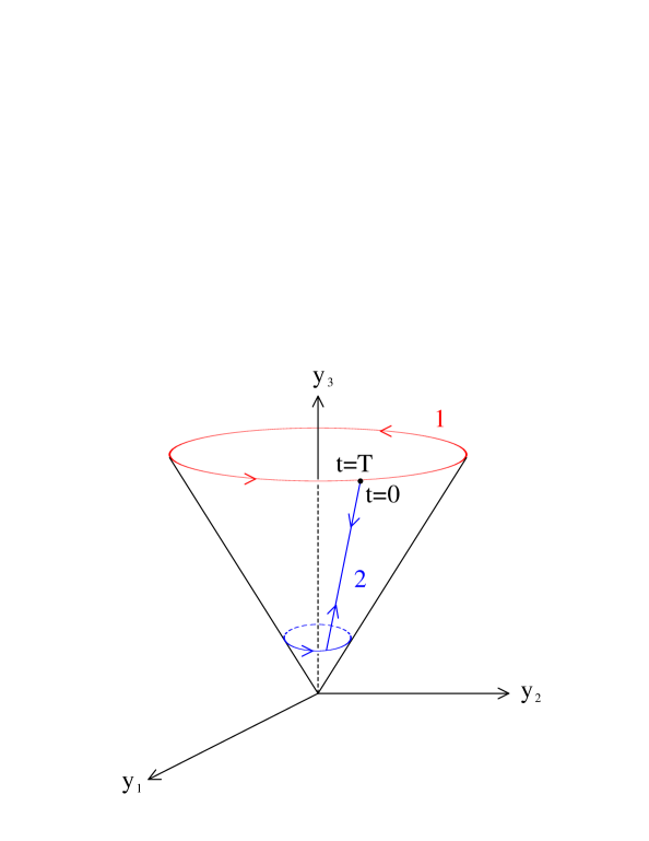
Fig. 1: The path 1 gives the conventional geometric phase as in (4.13) for a fixed finite $T$, whereas the path 2 gives a trivial geometric phase as in (4.15) for a fixed finite $T$. Note that both of the paths cover the same solid angle $2\pi(1-\cos\theta)$.

In our previous papers [24, 25], it has been analyzed in detail how the conventional formula (4.13) is modified if one deforms the contour in the parameter space for a fixed finite $T$. We here briefly comment on the main results. It was shown there that the amplitude in (4.13) is replaced by

$$\psi_{-}(0)^{\star}\psi_{-}(T) = \exp\{-\frac{i}{\hbar}\int_{C_{2}(0\rightarrow T)}dt[E(0)+y_{0}(t)-gr(t)-\hbar A^{k}_{--}(y)\dot{y}_{k}]\}$$ (4.22)

$$= \exp\{-\frac{i}{\hbar}\int_{C_{2}(0\rightarrow T)}dt[E(0)+y_{0}(t)-gr(t)]\}$$

by deforming the path 1 to the path 2 in the parameter space in Fig. 1. The path $C_{2}(0\rightarrow T)$ specifies the path 2 in Fig.1, and $v_{-}(y(T))=v_{-}(y(0))$ in the present choice of the gauge. Thus no geometric phase for the path $C_{2}$ for any fixed finite $T$. For $t=0$ or $t=T$, we start or end with the parameter region where the condition (4.10) for the adiabatic approximation is satisfied. But approaching the infinitesimal neighborhood of the origin where the level crossing takes place, the condition is no more satisfied and instead one has $Tgr\ll\hbar$. In this region of the parameter space, $\hat{H}_{eff}$ in (4.8) or (4.9) is replaced by

$$\hat{H}_{eff}(t) \simeq (E(0)+y_{0}(t))\hat{c}^{\dagger}_{+}\hat{c}_{+}$$ (4.23)

$$+ (E(0)+y_{0}(t))\hat{c}^{\dagger}_{-}\hat{c}_{-}-\hbar\dot{\varphi}\hat{c}^{\dagger}_{+}\hat{c}_{+}$$

where one performed a unitary transformation

$$\hat{b}_{m}=\sum_{n}U(\theta(t))_{mn}\hat{c}_{n}$$ (4.24)

with

$$U(\theta(t))=\left(\begin{array}[]{cc}\cos\frac{\theta}{2}&-\sin\frac{\theta}{2}\\ \sin\frac{\theta}{2}&\cos\frac{\theta}{2}\end{array}\right)$$ (4.27)

by assuming the validity of the two-level truncation in the infinitesimal neighborhood of the level crossing. The diagonalization of the geometric terms in (4.16) corresponds to the use of eigenfunctions

$$w_{+}=\left(\begin{array}[]{c}e^{-i\varphi}\\ 0\end{array}\right),\ \ \ \ \ w_{-}=\left(\begin{array}[]{c}0\\ 1\end{array}\right)$$ (4.32)

in the definition of geometric terms.

Based on this analysis, it was concluded in [24, 25] that the topological interpretation of the Berry’s phase fails in the practical Born-Oppenheimer approximation where $T$ is identified with the period of the slower dynamical system. Also, the appearance of a seemingly non-integrable phase factor is consistent with the integrability of the Schrödinger equation for a regular Hamiltonian.

Geometric phase for noncyclic evolution

We now analyze the geometric phase associated with a noncyclic evolution on the basis of the explicit two-level truncation. For the explicit example at hand, the starting gauge invariant formula (3.14) is given by

$$\psi_{-}(0;X(0))^{\star}\psi_{-}(T;X(T))$$

$$=v_{-}(y(0))^{\star}v_{-}(y(T))\exp\{-\frac{i}{\hbar}\int_{0}^{T}[E(0)+y_{0}(t)-gr(t)-\hbar A^{k}_{--}(y)\dot{y}_{k}]dt\}$$

$$=v_{-}(y(0))^{\star}v_{-}(y(T))\exp\{-\frac{i}{\hbar}\int_{0}^{T}[-\hbar A^{k}_{--}(y)\dot{y}_{k}]dt\}$$

$$\times\exp\{-\frac{i}{\hbar}\int_{0}^{T}[E(0)+y_{0}(t)-gr(t)]dt\}$$ (4.33)

by assuming the adiabatic approximation for the moment. Here again, the combination

$$v_{-}(y(0))^{\star}v_{-}(y(T))\exp\{-\frac{i}{\hbar}\int_{0}^{T}[-\hbar A^{k}_{--}(y)\dot{y}_{k}]dt\}$$ (4.34)

is invariant under hidden local gauge symmetry. For a noncycle evolution, there is no simple choice of gauge which eliminates the factor $v_{-}(y(0))^{\star}v_{-}(y(T))$ altogether.

In the present explicit example, we have by using (4.4)

$$v_{-}(y(0))^{\star}v_{-}(y(T))=\sin\frac{\theta(0)}{2}\sin\frac{\theta(T)}{2}e^{i(\varphi(0)-\varphi(T))}+\cos\frac{\theta(0)}{2}\cos\frac{\theta(T)}{2}.$$ (4.35)

By defining

$$v_{-}(y(0))^{\star}v_{-}(y(T))=|v_{-}(y(0))^{\star}v_{-}(y(T))|e^{i\Phi(T)}$$ (4.36)

one may perform a hidden local gauge transformation

$$v_{-}(y(t))\rightarrow v^{\prime}_{-}(t,y(t))=e^{-i\alpha_{-}(t)}v_{-}(y(t))$$ (4.37)

such that

$$\alpha_{-}(T)-\alpha_{-}(0)=\Phi(T).$$ (4.38)

The net result is then the prefactor in (4.20) is replaced by $|v_{-}(y(0))^{\star}v_{-}(y(T))|$ and the geometric phase is shifted by $\Phi(T)$. Namely, we have

$$\psi_{-}(0;X(0))^{\star}\psi_{-}(T;X(T))$$

$$=|v_{-}(y(0))^{\star}v_{-}(y(T))|$$

$$\times\exp\{-\frac{i}{\hbar}\int_{0}^{T}[E(0)+y_{0}(t)-gr(t)-\hbar A^{\prime\ k}_{--}(y)\dot{y}_{k}]dt\}$$

$$=|v_{-}(y(0))^{\star}v_{-}(y(T))|$$

$$\times\exp\{i\Phi(T)-\frac{i}{\hbar}\int_{0}^{T}[E(0)+y_{0}(t)-gr(t)-\hbar A^{k}_{--}(y)\dot{y}_{k}]dt\}.$$ (4.39)

The definition of the geometric phase

$$\int_{0}^{T}A^{\prime\ k}_{--}(y)\dot{y}_{k}dt=\int_{0}^{T}A^{k}_{--}(y)\dot{y}_{k}dt+\Phi(T)$$ (4.40)

gives an expression consistent with the basic idea of Pancharatnam [13]. See Section 5 and also Refs. [21, 22] for closely related analyses from the different points of view. Our formula contains all the information about the phase factor and that the gauge invariant definition of the phase of $\psi_{-}(0;X(0))^{\star}\psi_{-}(T;X(T))$ as a line integral is unique up to gauge transformations with $\alpha_{-}(T)=\alpha_{-}(0)$.

This quantity (4.26) is gauge invariant but path dependent in the parameter space for fixed $v_{-}(y(0))$, $v_{-}(y(T))$ and finite $T$. For example, for a path analogous to $C_{1}$ in Fig. 1 but now an open path (i.e., fixed $\theta$ and $\varphi(T)-\varphi(0)<2\pi$), one has (see also Ref. [22])

$$\psi_{-}(0;X(0))^{\star}\psi_{-}(T;X(T)) = |v_{-}(y(0))^{\star}v_{-}(y(T))|$$ (4.41)

$$\times \exp\{i\Phi(T)+i\frac{1}{2}(1-\cos\theta)(\varphi(T)-\varphi(0))\}$$

$$\times \exp\{-\frac{i}{\hbar}\int_{C_{1}}[E(0)+y_{0}(t)-gr(t)]dt\}.$$

For a path analogous to $C_{2}$ in Fig.1 but now an open path (i.e., fixed $\theta$ and $\varphi(T)-\varphi(0)<2\pi$), one has

$$\psi_{-}(0;X(0))^{\star}\psi_{-}(T;X(T)) = |v_{-}(y(0))^{\star}v_{-}(y(T))|$$ (4.42)

$$\times \exp\{i\Phi(T)+i(\varphi(T)-\varphi(0))\}$$

$$\times \exp\{-\frac{i}{\hbar}\int_{C_{2}}[E(0)+y_{0}(t)-gr(t)]dt\}.$$

If one sets $\varphi(T)=\varphi(0)+2\pi$ and $v_{-}(y(T))=v_{-}(y(0))$ (and thus $\Phi(T)=0$), these formulas are reduced to the previous formulas for a cyclic evolution.

Since we analyzed the behavior in the neighborhood of the level crossing, the $\vec{x}$ dependent part is factored out as in (4.12) and the important difference between the cyclic and noncyclic evolutions noted in (3.23) does not explicitly appear in the present example.

5 Comparison to gauge symmetry in the definition of generalized geometric phase

We here explain a basic conceptual difference between the hidden local gauge symmetry and a gauge symmetry (or equivalence class) which appears in the definition of generalized geometric phases by Aharonov and Anandan [8] and also by Samuel and Bhandari [13].

We first reformulate the treatments in these references from a view point of gauge symmetry by following Refs. [18, 19]. The analysis in Ref. [8] starts with the wave function satisfying

$$\int d^{3}x\psi(t,\vec{x})^{\star}\psi(t,\vec{x})=1,$$ (5.1)

and

$$\psi(T,\vec{x})=e^{i\phi}\psi(0,\vec{x})$$ (5.2)

with a real constant $\phi$. For simplicity we resrict our attention to the unitary time-development as in (5.1). The condition (5.1) then implies the existence of a hermitian Hamiltonian

$$i\hbar\frac{\partial}{\partial t}\psi(t,\vec{x})=\hat{H}(t,\frac{\hbar}{i}\frac{\partial}{\partial\vec{x}},\vec{x})\psi(t,\vec{x}).$$ (5.3)

The notion of generalized rays in refs. [8, 13] is based on the identification of all the vectors of the form

$$\{e^{i\alpha(t)}\psi(t,\vec{x})\}.$$ (5.4)

Note that they project $\psi(t,\vec{x})$ for each $t$, which means local in time unlike the conventional notion of rays which is based on constant $\alpha$  [28]. Since the conventional Schrödinger equation is not invariant under this equivalence class, we may consider an equivalence class of Hamiltonians

$$\{\hat{H}-\hbar\frac{\partial}{\partial t}\alpha(t)\}.$$ (5.5)

We next define an object

$$\Psi(t,\vec{x})\equiv\exp[i\int_{0}^{t}dt\int d^{3}x\psi(t,\vec{x})^{\star}i\frac{\partial}{\partial t}\psi(t,\vec{x})]\psi(t,\vec{x})$$ (5.6)

which satisfies

$$\Psi(0,\vec{x})=\psi(0,\vec{x}),$$

$$\int d^{3}x\Psi(t,\vec{x})^{\star}i\frac{\partial}{\partial t}\Psi(t,\vec{x})=0.$$ (5.7)

Under the equivalence class transformation (or gauge transfromation)

$$\psi(t,\vec{x})\rightarrow e^{i\alpha(t)}\psi(t,\vec{x}),$$ (5.8)

$\Psi(t,\vec{x})$ transforms as

$$\Psi(t,\vec{x})\rightarrow e^{\alpha(0)}\Psi(t,\vec{x}).$$ (5.9)

The quantity $\Psi(t,\vec{x})$ thus belongs to the same ray in the conventional sense under any gauge transformation. The properties (5.7) and (5.9) are valid independently of the precise form of Schrödinger equation (5.3), as we use only the property (5.1).

The gauge invariant quantity is then defined by

$$\Psi(0,\vec{x})^{\star}\Psi(T,\vec{x})=\psi(0,\vec{x})^{\star}\exp[i\int_{0}^{T}dt\int d^{3}x\psi(t,\vec{x})^{\star}i\frac{\partial}{\partial t}\psi(t,\vec{x})]\psi(T,\vec{x})$$ (5.10)

by following our general prescription (3.13). By a suitable gauge transformation

$$\psi(t,\vec{x})\rightarrow\tilde{\psi}(t,\vec{x})=e^{-i\alpha(t)}\psi(t,\vec{x})$$ (5.11)

with

$$\alpha(T)-\alpha(0)=\phi$$ (5.12)

we can make the prefactor in (5.10)

$$\psi(0,\vec{x})^{\star}\psi(T,\vec{x})\rightarrow\tilde{\psi}(0,\vec{x})^{\star}\tilde{\psi}(T,\vec{x})=e^{i\alpha(0)}\psi(0,\vec{x})^{\star}e^{-i\alpha(T)}\psi(T,\vec{x})=|\psi(0,\vec{x})|^{2}$$ (5.13)

real and positive for a cyclic evolution. The above gauge invariant quantity is then given by

$$\Psi(0,\vec{x})^{\star}\Psi(T,\vec{x}) = |\psi(0,\vec{x})|^{2}\exp[i\int_{0}^{T}dt\int d^{3}x\tilde{\psi}(t,\vec{x})^{\star}i\frac{\partial}{\partial t}\tilde{\psi}(t,\vec{x})]$$ (5.14)

and the factor on the exponential extracts all the information about the phase from the gauge invariant quantity. This definition of the gauge invariant phase agrees with the generalized geometric phase in [8] by noting $\tilde{\psi}(0,\vec{x})=\tilde{\psi}(T,\vec{x})$. The phase factor in (5.14) is invariant under a residual gauge symmetry with

$$\alpha(T)=\alpha(0).$$ (5.15)

The phase factor in (5.14) is also written as

$$\beta=\oint dt\int d^{3}x\tilde{\psi}(t,\vec{x})^{\star}i\frac{\partial}{\partial t}\tilde{\psi}(t,\vec{x})$$ (5.16)

which makes the invariance under the gauge transformation (5.15) manifest, but our basic formula (5.10) is invariant under a much larger class of gauge transformations. We can thus use the original variable $\psi$ which satisfies (5.3) and write (5.10) as

$$\Psi(0,\vec{x})^{\star}\Psi(T,\vec{x})=|\psi(0,\vec{x})|^{2}\exp[i\phi+\frac{i}{\hbar}\int_{0}^{T}dt\int d^{3}x\psi(t,\vec{x})^{\star}\hat{H}\psi(t,\vec{x})].$$ (5.17)

The phase on the exponential in (5.17) (and consequently, the phase in (5.14)) does not depend on the choice of the Hamiltonian in (5.5) since $\phi$ and the Hamiltonian are simultaneously changed by the parameter $\alpha(t)$. The factor $(-1/\hbar)\int_{0}^{T}dt\int d^{3}x\psi(t,\vec{x})^{\star}\hat{H}\psi(t,\vec{x})$ in (5.17) is called a “dynamical phase” in [8]. Note that the second relation in (5.7) does not play a major role in our formulation.

Next we comment on the generalized phase for a noncyclic evolution [13], namely, starting with (5.1) but the relation (5.2) is modified to

$$\psi(T,\vec{x})\neq e^{\phi}\psi(0,\vec{x})$$ (5.18)

for any space-independent $\phi$. We can still consider the object (5.6) and the gauge invariant quantity (5.10)

$$\Psi(0,\vec{x})^{\star}\Psi(T,\vec{x})=\psi(0,\vec{x})^{\star}\exp[i\int_{0}^{T}dt\int d^{3}x\psi(t,\vec{x})^{\star}i\frac{\partial}{\partial t}\psi(t,\vec{x})]\psi(T,\vec{x}).$$ (5.19)

The pre-factor $\psi(0,\vec{x})^{\star}\psi(T,\vec{x})$ now cannot be made real and positive for all $\vec{x}$ by any gauge transformation. One can still make the prefactor in the integrated quantity

$$\int d^{3}x\Psi(0,\vec{x})^{\star}\Psi(T,\vec{x})=\int d^{3}x\psi(0,\vec{x})^{\star}\psi(T,\vec{x})\exp[i\int_{0}^{T}dt\int d^{3}x\psi(t,\vec{x})^{\star}i\frac{\partial}{\partial t}\psi(t,\vec{x})]$$ (5.20)

real and positive. Namely, by defining

$$\int d^{3}x\psi(0,\vec{x})^{\star}\psi(T,\vec{x})=e^{i\Phi(T)}|\int d^{3}x\psi(0,\vec{x})^{\star}\psi(T,\vec{x})|,$$ (5.21)

one may consider a gauge transformation

$$\psi(t,\vec{x})\rightarrow\psi^{\prime}(t,\vec{x})=e^{-i\alpha(t)}\psi(t,\vec{x})$$ (5.22)

such that

$$\alpha(T)-\alpha(0)=\Phi(T).$$ (5.23)

One then obtains

$$\int d^{3}x\Psi(0,\vec{x})^{\star}\Psi(T,\vec{x})$$

$$=\int d^{3}x\psi^{\prime}(0,\vec{x})^{\star}\psi^{\prime}(T,\vec{x})\exp[i\int_{0}^{T}dt\int d^{3}x\psi^{\prime}(t,\vec{x})^{\star}i\frac{\partial}{\partial t}\psi^{\prime}(t,\vec{x})]$$

$$=|\int d^{3}x\psi^{\prime}(0,\vec{x})^{\star}\psi^{\prime}(T,\vec{x})|\exp[i\int_{0}^{T}dt\int d^{3}x\psi^{\prime}(t,\vec{x})^{\star}i\frac{\partial}{\partial t}\psi^{\prime}(t,\vec{x})]$$

$$=|\int d^{3}x\psi(0,\vec{x})^{\star}\psi(T,\vec{x})|\exp[i\int_{0}^{T}dt\int d^{3}x\psi^{\prime}(t,\vec{x})^{\star}i\frac{\partial}{\partial t}\psi^{\prime}(t,\vec{x})].$$ (5.24)

The factor on the exponential extracts all the information about the phase factor of the integrated gauge invariant quantity. One can also use the variable $\psi$, which satisfies the Schrödinger equation (5.3), in the gauge invariant quantity (5.20) and write it as

$$\int d^{3}x\Psi(0,\vec{x})^{\star}\Psi(T,\vec{x})$$

$$=|\int d^{3}x\psi(0,\vec{x})^{\star}\psi(T,\vec{x})|\exp[i\Phi(T)+\frac{i}{\hbar}\int_{0}^{T}dt\int d^{3}x\psi(t,\vec{x})^{\star}\hat{H}\psi(t,\vec{x})].$$ (5.25)

The phase factor in (5.25), which stands for the total phase increase of $\psi$ minus the “dynamical phase”, agrees with the defining equation of the generalized phase in [13]. Thus the phase on the exponential in (5.24) gives an alternative expression of the Pancharatnam phase difference as formulated in [13]. Note that the phase (5.24) is defined only for the integrated quantity as in (5.21), and it is invariant under the residual gauge symmetry satisfying (5.15).

Finally, we would like to compare the gauge symmetry appearing here to our hidden local gauge symmetry in the case of adiabatic approximation (but with finite $T$), for which the correspondence becomes most visible. The basic correspondences are

$$\psi(t,\vec{x}) \leftrightarrow v_{n}(\vec{x};X(t)),$$ (5.26)

and

$$i\hbar\frac{\partial}{\partial t}\psi(t,\vec{x})=\hat{H}(t,\frac{\hbar}{i}\frac{\partial}{\partial\vec{x}},\vec{x})\psi(t,\vec{x})$$

$$\leftrightarrow\hat{H}(\frac{\hbar}{i}\frac{\partial}{\partial\vec{x}},\vec{x},X(t))v_{n}(\vec{x};X(t))={\cal E}_{n}(t)v_{n}(\vec{x};X(t))$$

with the equivalence class

$$\{e^{i\alpha(t)}\psi(t,\vec{x})\} \leftrightarrow \{e^{i\alpha_{n}(t)}v_{n}(\vec{x};X(t))\}.$$ (5.28)

The quantity

$$\Psi(t,\vec{x})=\exp[i\int_{0}^{t}dt\int d^{3}x\psi(t,\vec{x})^{\star}i\frac{\partial}{\partial t}\psi(t,\vec{x})]\psi(t,\vec{x})$$ (5.29)

then corresponds to the quantity defined by

$$\Psi_{n}(\vec{x},t;X(t)) \equiv \exp\{\frac{i}{\hbar}\int_{0}^{t}{\cal E}_{n}(X(t))dt\}\psi_{n}(\vec{x},t;X(t))$$ (5.30)

$$= \exp[i\int_{0}^{t}\langle n|i\frac{\partial}{\partial t}|n\rangle dt]v_{n}(\vec{x};X(t)).$$

The physical observables in the cyclic evolution are then given by, respectively,

$$\Psi(0,\vec{x})^{\star}\Psi(T,\vec{x})=\psi(0,\vec{x})^{\star}\psi(T,\vec{x})\exp[i\int_{0}^{T}dt\int d^{3}x\psi(t,\vec{x})^{\star}i\frac{\partial}{\partial t}\psi(t,\vec{x})]$$ (5.31)

and

$$\Psi_{n}(\vec{x},0;X(0))^{\star}\Psi_{n}(\vec{x},T;X(T))$$

$$=v_{n}(0,\vec{x};X(0))^{\star}v_{n}(T,\vec{x};X(T))\exp[i\int_{0}^{T}\langle n|i\frac{\partial}{\partial t}|n\rangle dt]$$ (5.32)

where we used the notation $v_{n}(t,\vec{x};X(t))$ to emphasize the use of arbitrary gauge in the last expression.

The two formulations are thus very similar to each other, but there are several important differences. Most importantly, the true correspondence should be

$$\psi(t,\vec{x}) \leftrightarrow \psi_{n}(\vec{x},t;X(t))$$ (5.33)

instead of (5.26), since both of $\psi(t,\vec{x})$ and $\psi_{n}(\vec{x},t;X(t))$ in (2.23) stand for the Schrödinger probability amplitudes. As a consequence of the difference between (5.26) and (5.33), a crucial difference in the conceptual level appears in the definition of equivalence class (or gauge symmetry). The hidden local gauge symmetry is consistent with the eigenvalue equation (5.27) and in fact it is an exact symmetry of quantized theory as was explained in Section 3. The Schrödinger amplitude $\psi_{n}(\vec{x},t;X(t))$ is transformed under the hidden local symmetry as

$$\psi_{n}(\vec{x},t;X(t))\rightarrow\psi^{\prime}_{n}(\vec{x},t;X(t))=e^{i\alpha_{n}(0)}\psi_{n}(\vec{x},t;X(t))$$ (5.34)

as is shown in (3.10). This hidden local symmetry is exactly preserved in the adiabatic approximation. (Although the Schrödinger equation is satisfied only approximately in the adiabatic approximation, it is a nature of the approximation.)

In contrast, the equivalence class in the generalized definition (5.8) changes the form of the Schrödinger equation, and thus not a symmetry of quantized theory in the conventional sense. In fact, the constant phase in $e^{i\alpha}\psi(t,\vec{x})$ does not change physics since it provides an overall constant phase for the state vector at all the times, but the time-dependent phase in $e^{i\alpha(t)}\psi(t,\vec{x})$ generally changes physics by providing different phases at different times for the state vector. If one should take the equivalence class (5.4) literally, the conventional geometric phase would lose much of its significance as is exemplified by the fact that the product of Schrödinger wave functions $\psi(0,\vec{x})^{\star}\psi(T,\vec{x})$ in (5.13) can be made real and positive by a suitable choice of gauge, though not all is lost as the $\vec{x}$-dependence of $\psi(t,\vec{x})$ retains the information of the Hamiltonian. By taking $\Psi(t,\vec{x})$ in (5.6) as a basic physical object, which is transformed by a constant phase under any gauge transformation, one can identify the generalized geometric phases in [8, 13] by the consideration of gauge invariance alone, as we have explained in this section by following [18, 19]. The line integral along the “vertical” curve in [13] corresponds to the general gauge transformation (5.11) or (5.22), and the gauge symmetry which preserves the generalized geometric phases in [8, 13] corresponds to the residual gauge symmetry (5.15). These generalized geometric phases describe certain intrinsic properties of the class of Hamiltonians in (5.5) as is explained in detail in [8, 13]. See also Refs. [18, 19, 20] for the further elaboration on these generalized geometric phases.

In comparison, the original analysis of holonomy by Simon [2] is based on the gauge transformation

$$\psi(t,\vec{x})\rightarrow e^{i\alpha(X(t))}\psi(t,\vec{x})$$ (5.35)

in the precise adiabatic limit (with $T\rightarrow\infty$) where the time-dependence of $X(t)$ is negligible. In the precise adiabatic limit, it is known that the two formulations in (5.27) (when interpreted in the sense of (5.35)) essentially coincide [8] and thus two gauge symmetries with quite different origins give rise to the same result.

6 Discussion

The analysis of geometric phases is reduced to the familiar diagonalization of the Hamiltonian in the second quantized formulation. The hidden local gauge symmetry, which is an exact symmetry of quantum theory, becomes explicit in this formulation and we analyzed its full implications for cyclic and noncyclic evolutions in the study of geometric phases. We have shown that the general prescription of Pancharatnam is consistent with the analysis on the basis of the hidden local gauge symmetry. When one analyzes processes which are adiabatic only approximately, as in the practical Born-Oppenheimer approximation, the geometric phases cease to be purely geometrical. The notions of parallel transport and holonomy then become somewhat subtle, but our hidden local gauge symmetry is still exact and useful. The hidden local symmetry as formulated in this paper can thus provide a basic concept alternative to the notions of parallel transport and holonomy to analyze geometric phases associated with level crossing. We have also explained a basic difference between the hidden local gauge symmetry and a gauge symmetry used in the definition of generalized geometric phases.

The notion of geometric phases is known to be exactly or approximately associated with a wide range of physical phenomena [29, 30]. However, it is our opinion that the crucial differences of various physical phenomena, which are loosely associated with geometric phases, should be explicitly and precisely stated. The topological triviality of geometric phases associated with level crossing for any finite $T$, which is crucially different from the exact topological property of the Aharonov-Bohm phase, is one of those examples.

I thank S. Deguchi for helpful discussions and A. Hosoya for asking a connection of our formulation to that in Ref. [8]. I also thank O. Bar for calling the non-level crossing theorem to my attention.

References

[1]
M.V. Berry, Proc. Roy. Soc. Ser. A392, 45 (1984).
[2]
B. Simon, Phys. Rev. Lett. 51, 2167 (1983).
[3]
A.J. Stone, Proc. Roy. Soc. Ser. A351, 141 (1976).
[4]
H. Longuet-Higgins, Proc. Roy. Soc. Ser. A344, 147 (1975).
[5]
F. Wilczek and A. Zee, Phys. Rev. Lett. 52, 2111 (1984).
[6]
H. Kuratsuji and S. Iida, Prog. Theor. Phys. 74, 439
(1985).
[7]
J. Anandan and L. Stodolsky, Phys. Rev. D35, 2597 (1987).
[8]
Y. Aharonov and J. Anandan, Phys. Rev. Lett. 58, 1593
(1987).
[9]
M.V. Berry, Proc. Roy. Soc. Ser. A414, 31 (1987).
[10]
Y. Lyanda-Geller, Phys. Rev. Lett. 71, 657 (1993).
[11]
N. Manini and F. Pistolesi, Phys. Rev. Lett. 85, 3067
(2000).
[12]
R. Bhandari, Phys. Rev. Lett. 88, 100403 (2002).
[13]
J. Samuel and R. Bhandari, Phys. Rev. Lett. 60, 2339
(1988).
[14]
S. Pancharatnam, Proc. Indian Acad. Sci. A44, 247 (1956),
reprinted in Collected Works of S. Pancharatnam, (Oxford
University Press, Oxford, 1975).
[15]
S. Ramaseshan and R. Nityananda, Curr. Sci. 55, 1225
(1986).
[16]
M.V. Berry, J. Mod. Optics 34, 1401 (1987).
[17]
G. Giavarini, E. Gozzi, D. Rohrlich and W.D. Thacker,
Phys. Lett. A 138, 235 (1989).
[18]
I.J.R. Aitchison and K. Wanelik, Proc. Roy. Soc. Ser. A439,
25 (1992).
[19]
N. Mukunda and R. Simon, Ann. Phys. (N.Y.) 228, 205 (1993).
[20]
A.K. Pati, Phys. Rev. A52, 2576 (1995).
[21]
A.K. Pati, Ann. Phys. (N.Y.) 270, 178 (1998).
[22]
G. Garcia de Polavieja and E. Sjöqvist, Am. J. Phys.
66, 431 (1998).
[23]
A. Mostafazadeh, J. Phys. A32, 8157 (1999).
[24]
K. Fujikawa, Mod. Phys. Lett. A20, 335 (2005),
quant-ph/0411006.
[25]
S. Deguchi and K. Fujikawa, ”Second quantized formulation of
geometric phases” (to appear in Phys. Rev. A), hep-th/0501166.
[27]
K. Fujikawa, Phys. Rev. Lett. 42, 1195 (1979); Phys.
Rev. D21, 2848 (1980).
[28]
R.F. Streater and A.S. Wightman, PCT, Spin and Statistics and All That (W.A. Benjamin, Inc., New York, 1964).
[29]
A. Shapere and F. Wilczek, ed., Geometric Phases in
Physics (World Scientific, Singapore, 1989), and
papers reprinted therein.
[30]
For a recent account of geometric phases see, for
example, D. Chruscinski and A. Jamiolkowski, Geometric
Phases in Classical and Quantum Mechanics (Birkhauser, Berlin,
2004).