Abstract

We study K$\ddot{\mbox{a}}$hler gravity on local $SU(N)$ geometry and describe precise correspondence with certain supersymmetric gauge theories and random plane partitions. The local geometry is discretized, via the geometric quantization, to a foam of an infinite number of gravitational quanta. We count these quanta in a relative manner by measuring a deviation of the local geometry from a singular Calabi-Yau threefold, that is a $A_{N-1}$ singularity fibred over $\mathbb{P}^{1}$. With such a regularization prescription, the number of the gravitational quanta becomes finite and turns to be the perturbative prepotential for five-dimensional $\mathcal{N}=1$ supersymmetric $SU(N)$ Yang-Mills. These quanta are labelled by lattice points in a certain convex polyhedron on $\mathbb{R}^{3}$. The polyhedron becomes obtainable from a plane partition which is the ground state of a statistical model of random plane partition that describes the exact partition function for the gauge theory. Each gravitational quantum of the local geometry is shown to consist of $N$ unit cubes of plane partitions.

1 Introduction

A surprising interpretation of a possible connection [1] between topological strings on Calabi-Yau threefolds and statistical models of crystal melting, known as random plane partitions, has been advocated. It is conjectured [2] that the statistical model is nothing but a quantum gravitational path integral involving fluctuations of K$\ddot{\mbox{a}}$hler geometry and topology, by interpreting plane partitions as gravitational quantum foams in K$\ddot{\mbox{a}}$hler gravity [3], that is the target space field theory of topological $A$-model strings [4]. It is shown [2] that the topological vertex counting [5] of the $A$-model partition function on a local toric Calabi-Yau threefold, which involves from the worldsheet viewpoint sums over holomorphic maps to the target space, is reproduced from quantum fluctuations of K$\ddot{\mbox{a}}$hler gravity on the fixed macroscopic background by assuming that the fluctuations are quantized in the unit of the string coupling constant $g_{st}$.

The topological vertex countings are known [6] to bring about the gauge instanton contributions to the exact partition functions [7] for supersymmetric gauge theories. However, the exact partition functions themselves are fully reproduced [8] by random plane partitions. Thinking over the conjecture, this indicates that even background geometries in K$\ddot{\mbox{a}}$hler gravity also have a microscopic origin in the statistical models, given by certain plane partitions, and emerge from the quantum foams by taking the semi-classical limit $g_{st}\rightarrow 0$. Further developing consideration along this line might lead to an explanation of microscopic generation of the target spaces for perturbative string theories. From the gauge theory viewpoint, it could deepen our understanding of the geometric engineering [9] and will provide another formulation for gauge/gravity correspondence in string theories.

In this article we take the first step towards that direction. We study K$\ddot{\mbox{a}}$hler gravity on local $SU(N)$ geometry and describe precise correspondence with certain supersymmetric gauge theories and random plane partitions. The local geometry is a noncompact toric Calabi-Yau threefold and is considered as an ALE space with $A_{N-1}$ singularity fibred over $\mathbb{P}^{1}$. When K$\ddot{\mbox{a}}$hler forms $\omega$ on algebraic varieties are quantized in the unit of $g_{st}$, one is naturally led to an idea of geometric quantization [10] of the varieties. The geometric quantization requires a holomorphic line bundle $L$ on a variety $X$ whose first Chern class is equal to the quantized K$\ddot{\mbox{a}}$hler class. Physical states of the theory are given by the global sections, and the physical Hilbert space $\mathcal{H}_{\omega}$ is identified with

$$\mathcal{H}_{\omega}=H^{0}(X,\,L)\,.$$ (1.1)

In the quantization, we regard the variety of dimension $n$, equipped with the quantized K$\ddot{\mbox{a}}$hler form, as a phase space. The least volume measurable quantum mechanically on this phase space is $\sim g_{st}^{n}$. The variety could be divided into pieces of the minimal volume, where each piece corresponds to a gravitational quantum, and thereby discretized to a foam of gravitational quanta. It is clear that the number of the quanta is given by $\mbox{dim}\,\mathcal{H}_{\omega}$ and estimated as $\mbox{Vol}(X)/g_{st}^{n}$.

Thanks to that the local geometry is a toric variety, the gravitational quanta turn to be labelled by lattice points in a certain convex polyhedron on $\mathbb{R}^{3}$. Reflecting the noncompactness of the geometry, the polyhedron is unbounded and the number of the lattice points becomes infinite. Hence the physical Hilbert space is infinite dimensional. A convenient way to manipulate such an infinity is to count the quanta in a relative sense rather than in an absolute sense. We introduce the regularized dimensions by counting the deviation from a singular Calabi-Yau threefold, that is a $A_{N-1}$ singularity fibred over $\mathbb{P}^{1}$.

The regularized dimensions turns to be a perturbative prepotential for five-dimensional supersymmetric gauge theory at the semi-classical limit $g_{st}\rightarrow 0$. This is a manifestation of gauge/gravity correspondence.

A possible relation between the quantized $SU(N)$ geometry and five-dimensional $\mathcal{N}=1$ supersymmetric $SU(N)$ Yang-Mills is suggested in [8] through the study of a statistical model of random plane partitions. After translating the quantized K$\ddot{\mbox{a}}$hler parameters into the gauge theory parameters as in [8], the regularized dimensions satisfies

$$g_{st}\cdot\mbox{dim}\,\mathcal{H}_{\omega}=-\frac{1}{\hbar^{2}}\Bigl{\{}\mathcal{F}^{pert}_{\mbox{{\scriptsize 5dSYM}}}+O(\hbar)\Bigr{\}}\,,$$ (1.2)

where $\mathcal{F}^{pert}_{\mbox{{\scriptsize 5dSYM}}}$ is the perturbative prepotential for five-dimensional $\mathcal{N}=1$ supersymmetric $SU(N)$ Yang-Mills with the Chern-Simons term [11, 12]. The five-dimensional theory is living on $\mathbb{R}^{4}\times S^{1}$, where the radius $R$ of the circle in the fifth dimension is large (the large radius limit). The parameter $\hbar$ plays the similar role as $g_{st}$ in the statistical model, and relates with the string coupling constant by $g_{st}=2R\hbar$. The Chern-Simons coupling constant is quantized in accord with the framing of the local geometry that labels possible fibrations over $\mathbb{P}^{1}$. The above might lead a rationale for the geometric engineering [9], which originally dictates that four-dimensional $\mathcal{N}=2$ supersymmetric $SU(N)$ Yang-Mills is realized by the $SU(N)$ geometry.

It is shown in [8, 13] that a certain model of random plane partitions gives the exact partition function [7] for the five-dimensional Yang-Mills. It is often convenient to identify plane partitions with the three-dimensional Young diagrams. By regarding each cube as a lattice point, the three-dimensional diagrams can be interpreted as the sets of lattice points in $\mathbb{R}^{3}$.

The ground state of the statistical model is called ground plane partition. The ground state energy turns out to relate with the perturbative prepotential by

$$E_{min}=\frac{1}{\hbar^{2}}\Bigl{\{}\mathcal{F}^{pert}_{\mbox{{\scriptsize 5dSYM}}}+O(\hbar)\Bigr{\}}\,.$$ (1.3)

The ground plane partition is determined uniquely from a ground partition. It is well known that partitions are realized in the Fock representation of two-dimensional complex fermions. Ground partitions appear naturally in an alternative realization of the Fock representation by exploiting $N$ component complex fermions and get connected to K$\ddot{\mbox{a}}$hler gravities on a $A_{N-1}$ singularity or the ALE space [8].

The ground plane partition leads to the quantum foam of local $SU(N)$ geometry. In counting the deviation from the singular Calabi-Yau threefold, one needs to introduce another convex polyhedron which includes the original one. The complement, that becomes a bounded three-dimensional solid, measures the deviation. This three-dimensional solid becomes obtainable from the ground plane partition at the semi-classical limit $\hbar\rightarrow 0$. The lattice which is used to label the gravitational quanta becomes a sublattice of degree $N$ of the lattice on which plane partitions are drawn. It follows that each gravitational quantum of the $SU(N)$ geometry consists of $N$ cubes of plane partitions.

This article is organized as follows; we begin Section 2 by a brief review on toric geometries, and give the toric description of local $SU(N)$ geometry. We study K$\ddot{\mbox{a}}$hler gravity on the local geometry in Section 3. The regularized dimensions of the physical Hilbert space is introduced by using algebraic toric geometry. The discretization of the local geometry into the foam of gravitational quanta is explained by communicating with the gauged linear $\sigma$-model description of the geometry. We also argue the validity of the regularized dimensions by showing how the definition fits to the Riemann-Roch formula. In Section 4 we examine the statistical model of random plane partitions and show how the K$\ddot{\mbox{a}}$hler gravity is seen by the random plane partitions. In Appendix we summarize two-dimensional complex fermions which are used in the last section.

2 Local $SU(N)$ Geometry as Toric Variety

We start with a brief review on toric varieties. Further information on algebraic toric geometries can be found in [14] and [15]. We then provide a toric description of local $SU(N)$ geometry, which is a noncompact toric Calabi-Yau threefold.

2.1 A review on toric varieties

A toric variety $X$ is an algebraic variety that contains an algebraic torus $T$ as a dense open subset, equipped with an action of $T$ on $X$ which extends the natural action of $T$ on itself. An $n$-dimensional toric variety is constructed from a $\mathbb{Z}^{n}$-lattice $N$ and a fan $\Delta$, which is a collection of rational strongly convex polyhedral cones $\sigma$ in $N_{\mathbb{R}}=N\otimes\mathbb{R}$, satisfying the conditions; i) every face of a cone in $\Delta$ is also a cone in $\Delta$, and ii) the intersection of two cones in $\Delta$ is a face of each. A rational strongly convex polyhedral cone in $N_{\mathbb{R}}$ is a cone with apex at the origin, generated by a finite number of vectors in the lattice $N$. Such a cone will be called simply as a cone in $N$.

Let $M$ denote the dual lattice and $\langle\,,\,\rangle$ be the dual pairing. For a cone $\sigma$ in $N$, the dual cone $\sigma^{\vee}$ is the set of vectors in $M_{\mathbb{R}}=M\otimes\mathbb{R}$ which are nonnegative on $\sigma$. This gives a finitely generated commutative semigroup which is a sub-semigroup of the dual lattice.

$$\mathcal{S}_{\sigma}=M\cap\sigma^{\vee}=\Bigl{\{}u\in M\,;\,\langle u,v\rangle\geq 0\,\,\,\mbox{for}\,\,\forall v\in\sigma\Bigr{\}}.$$ (2.1)

The corresponding group ring $\mathbb{C}[\mathcal{S}_{\sigma}]$ is a finitely generated commutative algebra. As a complex vector space the group ring has a basis $\chi_{m}$, where $m$ runs over $\mathcal{S}_{\sigma}$, with multiplication $\chi_{m}\cdot\chi_{m^{\prime}}=\chi_{m+m^{\prime}}$. Generators for $\mathcal{S}_{\sigma}$ provide generators for $\mathbb{C}[\mathcal{S}_{\sigma}]$. This commutative algebra determines an affine variety $U_{\sigma}$ by

$$U_{\sigma}=\mbox{Spec}(\mathbb{C}[\mathcal{S}_{\sigma}])\,.$$ (2.2)

The points correspond to semigroup homomorphisms from $\mathcal{S}_{\sigma}$ to $\mathbb{C}$, where $\mathbb{C}$ is understood as an abelian semigroup by multiplication. Thus we can write

$$U_{\sigma}=\mbox{Hom}_{sgr}(\mathcal{S}_{\sigma},\mathbb{C}).$$ (2.3)

For a semigroup homomorphism $\alpha$ from $\mathcal{S}_{\sigma}$ to $\mathbb{C}$ and $m\in\mathcal{S}_{\sigma}$, the value of $\chi_{m}$ at the point $\alpha$ is given by $\chi_{m}(\alpha)=\alpha(m)$. The algebraic torus is identified with $\mbox{Hom}_{gr}(M,\mathbb{C}^{\ast})$, and acts on the affine variety as

$$\begin{array}[]{ccc}T\times U_{\sigma}&\longrightarrow&U_{\sigma}\\[5.69054pt] (t,\alpha)&\longmapsto&t\circ\alpha\,,\end{array}$$ (2.6)

where $t\circ\alpha(m)\equiv t(m)\alpha(m)$ for all $m\in\mathcal{S}_{\sigma}$.

Let us look at a basic example. Let $e_{1},\cdots,e_{n}$ be a basis for $N$ and $e_{1}^{*},\cdots,e_{n}^{*}$ be the dual basis for $M$. Let $\sigma$ be the $k$-dimensional cone with the generators $e_{1},\cdots,e_{k}$. Then $\mathcal{S}_{\sigma}=\mathbb{Z}_{\geq 0}e^{*}_{1}+\cdots+\mathbb{Z}_{\geq 0}e^{*}_{k}+\mathbb{Z}e^{*}_{k+1}+\cdots+\mathbb{Z}e^{*}_{n}$. Write $X_{i}=\chi_{e_{i}^{*}}$. The group ring becomes $\mathbb{C}[\mathcal{S}_{\sigma}]=\mathbb{C}\bigl{[}X_{i}\,(1\leq i\leq k),\,X_{j},X_{j}^{-1}\,(k+1\leq j\leq n)\bigr{]}$. Therefore we obtain $U_{\sigma}=(\mathbb{C})^{k}\times(\mathbb{C}^{\ast})^{n-k}$. This shows that if $\sigma$ is generated by $k$ elements which can be completed to a basis for $N$, the corresponding affine toric variety $U_{\sigma}$ is a product $(\mathbb{C})^{k}\times(\mathbb{C}^{\ast})^{n-k}$. In particular, such affine toric varieties are nonsingular.

The toric variety $X_{\Delta}$ is obtained from a fan $\Delta$ by taking a disjoint union of the affine toric varieties $U_{\sigma}$ for each $\sigma\in\Delta$, and patching them together by using the identity $U_{\sigma}\cap U_{\tau}=U_{\sigma\,\cap\,\tau}$.

$$X_{\Delta}=\bigcup_{\sigma\in\Delta}U_{\sigma}.$$ (2.7)

The torus actions on the affine varieties are compatible with one another by the gluing, and give rise to the torus action on $X_{\Delta}$. The zero-dimensional cone $\{0\}$ determines the affine variety $U_{\{0\}}=\mbox{Hom}_{gr}(M,\mathbb{C}^{\ast})$. It is nothing but the torus which becomes a dense open subset of $X_{\Delta}$.

It is possible to decompose a toric variety into a disjoint union of its orbits by the torus action. It appears one such orbit $O_{\tau}$ for each cone $\tau\in\Delta$. Let $\tau^{\perp}$ be the set of vectors in $M_{\mathbb{R}}$ which vanish on $\tau$. For any cone $\sigma$ that contains $\tau$ as a face, we consider the embedding

$$\mbox{Hom}_{sgr}(\mathcal{S}_{\sigma}\cap\tau^{\perp},\mathbb{C}^{\ast})\,\hookrightarrow\,U_{\sigma}$$ (2.8)

given by extension by zero on the complement $\mathcal{S}_{\sigma}\setminus(\mathcal{S}_{\sigma}\cap\tau^{\perp})$. By the embedding, $\mbox{Hom}_{sgr}(\mathcal{S}_{\sigma}\cap\tau^{\perp},\mathbb{C}^{\ast})$ becomes an orbit of the torus action (2.6). The strong convexity of $\sigma$, which is translated to the nondegeneracy $\mathcal{S}_{\sigma}+(-\mathcal{S}_{\sigma})=M$, makes the orbit identical to $\mbox{Hom}_{gr}(M\cap\tau^{\perp},\mathbb{C}^{\ast})$, which is $(\mathbb{C}^{\ast})^{n-k}$ if $\mbox{dim}\,\tau=k$. By letting

$$O_{\tau}=\mbox{Hom}_{gr}(M\cap\tau^{\perp},\mathbb{C}^{\ast}),$$ (2.9)

we see that each affine variety in (2.7) is a disjoint union of those orbits $O_{\tau}$ for which $\sigma$ contains $\tau$ as a face.

$$U_{\sigma}=\coprod_{\tau<\sigma}O_{\tau},$$ (2.10)

where $\tau<\sigma$ means that $\tau$ is a face of $\sigma$. Therefore $X_{\Delta}$ becomes a disjoint union of the orbits $O_{\sigma}$ over $\sigma\in\Delta$.

$$X_{\Delta}=\coprod_{\sigma\in\Delta}O_{\sigma}\,.$$ (2.11)

The closure of $O_{\sigma}$ becomes a closed subvariety of $X_{\Delta}$ which is again a toric variety. Let us denote the closure of $O_{\sigma}$ by $V(\sigma)$. This turns out to be a disjoint union of the orbits $O_{\tau}$ for which $\tau$ contains $\sigma$ as a face.

$$V(\sigma)=\coprod_{\tau>\sigma}O_{\tau}.$$ (2.12)

2.2 Local $SU(N)$ geometry as toric variety

We provide a toric description of local $SU(N)$ geometry. Local $SU(N)$ geometry is an ALE space with $A_{N-1}$ singularity fibred over $\mathbb{P}^{1}$. The fibration over $\mathbb{P}^{1}$ is labeled by an integer $k_{\mbox{\tiny{C.S.}}}\in[0,\,N]$, which is called the framing.

Let $N$ be a three-dimensional lattice with generators $e_{1},e_{2}$ and $e_{3}$. Let $v_{i}$ be the following $N+3$ elements in $N$.

$$v_{i}=ie_{2}+e_{3}\hskip 11.38109pt(0\leq i\leq N),\hskip 17.07164ptv_{N+1}=e_{1}+e_{3},\hskip 17.07164ptv_{N+2}=-e_{1}+\widetilde{k}_{\mbox{\tiny{C.S.}}}e_{2}+e_{3},$$ (2.13)

where $\widetilde{k}_{\mbox{\tiny{C.S.}}}\equiv N-k_{\mbox{\tiny{C.S.}}}$. We introduce three-dimensional cones $\sigma_{0},\sigma_{1},\,\cdots\,,\sigma_{2N-1}$ in $N$ as follows.

$$\sigma_{2k} = \mathbb{R}_{\geq 0}v_{k}+\mathbb{R}_{\geq 0}v_{k+1}+\mathbb{R}_{\geq 0}v_{N+1},$$

$$\sigma_{2k+1} = \mathbb{R}_{\geq 0}v_{k}+\mathbb{R}_{\geq 0}v_{k+1}+\mathbb{R}_{\geq 0}v_{N+2}.$$ (2.14)

All these cones and their faces constitute the fan $\Delta$ which is relevant to describe local $SU(N)$ geometry with the framing $k_{\mbox{\tiny{C.S.}}}$. See Figure 1. Generators for any cone $\sigma\in\Delta$ are taken from the elements $v_{i}$. It is easy to see that these generators can be always completed to a basis for $N$. This shows that the corresponding affine variety $U_{\sigma}$ is nonsingular. Therefore the corresponding toric variety is nonsingular.

\psfrag{r0}{$\rho_{0}$}\psfrag{r1}{$\rho_{1}$}\psfrag{r2}{$\rho_{2}$}\psfrag{r3}{$\cdots$}\psfrag{r4}{$\rho_{N}$}\psfrag{rN+1}{$\rho_{N+1}$}\psfrag{rN+2}{$\rho_{N+2}$}\psfrag{s0}{$\sigma_{0}$}\psfrag{s1}{$\sigma_{1}$}\psfrag{s2}{$\sigma_{2}$}\psfrag{s3}{$\sigma_{3}$}\psfrag{s4}{}\psfrag{s5}{}\psfrag{s6}{$\sigma_{2N-2}$}\psfrag{s7}{$\sigma_{2N-1}$}\psfrag{o}{$0$}\includegraphics[scale={.8}]{fan_3d.eps}

Figure 1: Cones relevant to describe the $SU(N)$ geometry.

There exist $N$ linear relations among $v_{i}$ owing to the dimensionality.

$$v_{i-1}-2v_{i}+v_{i+1} = 0\hskip 22.76219pt(1\leq i\leq N-1)\,,$$

$$(\widetilde{k}_{\mbox{\tiny{C.S.}}}-2)v_{0}-\widetilde{k}_{\mbox{\tiny{C.S.}}}v_{1}+v_{N+1}+v_{N+2} = 0\,.$$ (2.15)

These relations are conveniently expressed in the matrix form by

$$\bigl{(}\hskip 2.84526ptv_{0},\cdots,v_{i},\cdots,v_{N+2}\hskip 2.84526pt\bigr{)}\,Q=0\,,$$ (2.16)

where

$$Q=\bigl{(}Q_{ia}\bigr{)}_{0\leq i\leq N+2,\,1\leq a\leq N}=\left(\begin{array}[]{cccccc}1&&&&\widetilde{k}_{\mbox{\tiny{C.S.}}}-2\\ -2&1&&&-\widetilde{k}_{\mbox{\tiny{C.S.}}}\\ 1&-2&\ddots&&\\ &1&\ddots&1&\\ &&\ddots&-2&0\\ &&&1&0\\ &&&&1\\ &&&&1\end{array}\right)\,.$$ (2.25)

The matrix $Q$ is identified [16] with a charge matrix which appears in the gauged linear $\sigma$-model description of local $SU(N)$ geometry.

For the later convenience we name the lower dimensional cones of $\Delta$. There appear one-dimensional cones $\rho_{0},\rho_{1},\,\cdots\,,\rho_{N+2}$, and two-dimensional cones $\gamma_{0},\gamma_{1},\,\cdots\,,\gamma_{3N+1}$. See Figure 1. They are given by

$$\rho_{i} = \mathbb{R}_{\geq 0}v_{i}\,,$$ (2.26)

$$\gamma_{3k} = \mathbb{R}_{\geq 0}v_{k}+\mathbb{R}_{\geq 0}v_{N+1}\,,$$

$$\gamma_{3k+1} = \mathbb{R}_{\geq 0}v_{k}+\mathbb{R}_{\geq 0}v_{N+2}\,,$$ (2.27)

$$\gamma_{3k+2} = \mathbb{R}_{\geq 0}v_{k}+\mathbb{R}_{\geq 0}v_{k+1}\,.$$

3 K$\ddot{\mbox{a}}$hler Gravity on Local $SU(N)$ Geometry

One obtains local $SU(N)$ geometry from the fan $\Delta=\bigl{\{}\sigma_{i},\,\gamma_{j},\,\rho_{k},\,\{0\}\bigr{\}}$ as a nonsingular toric variety $X_{\Delta}$. The two-dimensional cones $\gamma_{j}$ determine two-cycles $V(\gamma_{j})$. Among them we can choose $V(\gamma_{2})$ and $V(\gamma_{3k})$ with $1\leq k\leq N-1$, as a basis for $H_{2}(X_{\Delta},\mathbb{Z})$. Vanishing cycles of the fibred $A_{N-1}$ singularity are $V(\gamma_{3k})$. The base $\mathbb{P}^{1}$ is identified with $V(\gamma_{2})$ for the case of $k_{\mbox{\tiny{C.S.}}}=N$. One needs a slight modification for other framings.

Let $\omega$ be a K$\ddot{\mbox{a}}$hler two-form. The K$\ddot{\mbox{a}}$hler class $[\omega]\in H^{2}(X_{\Delta},\mathbb{R})$ is specified by the K$\ddot{\mbox{a}}$hler volumes of the two-cycles.

$$t_{k}\equiv\int_{V(\gamma_{3k})}\!\!\!\omega\,,\hskip 22.76219ptt_{N}\equiv\int_{V(\gamma_{2})}\!\!\!\omega\,,$$ (3.1)

where the classical parameters $t$ take nonnegative real numbers. In what follows, as suggested in [2], we assume that K$\ddot{\mbox{a}}$hler forms are quantized in the unit of $g_{st}$.

$$\frac{1}{g_{st}}\bigl{[}\omega\bigr{]}\,\in H^{2}(X_{\Delta},\mathbb{Z})\,.$$ (3.2)

They are specified by the quantized parameters $T$ which take nonnegative integers.

$$T_{k}\equiv\frac{1}{g_{st}}\int_{V(\gamma_{3k})}\!\!\!\omega \in\mathbb{Z}_{\geq 0}\hskip 14.22636pt(k=1,2,\,\cdots\,,N-1)\,,$$

$$T_{N}\equiv\frac{1}{g_{st}}\int_{V(\gamma_{2})}\!\!\!\omega \in\mathbb{Z}_{\geq 0}\,.$$ (3.3)

When the K$\ddot{\mbox{a}}$hler forms on algebraic varieties are quantized, one is naturally led to an idea of geometric quantization of the varieties. The power of geometric quantizations for gravity theories may be seen in three-dimensional Chern-Simons gravity [17] as investigated in [18].

3.1 Geometric quantization of local $SU(N)$ geometry

The geometric quantization requires, first of all, a holomorphic line bundle $L$ whose first Chern class is equal to the quantized K$\ddot{\mbox{a}}$hler class.

$$c_{1}(L)=\frac{1}{g_{st}}\bigl{[}\omega\bigr{]}\,.$$ (3.4)

Let $Pic(X)$ be the group of all line bundles on an algebraic variety $X$, modulo isomorphism. For each $[L]\in Pic(X)$ we can associate the first Chern class of the line bundle. This gives a map from $Pic(X)$ to $H^{2}(X,\mathbb{Z})$. In the present toric geometry the map turns to be bijective, and $Pic(X_{\Delta})$ becomes isomorphic to $H^{2}(X_{\Delta},\mathbb{Z})$.

$$\begin{array}[]{ccc}Pic(X_{\Delta})&\stackrel{{\scriptstyle\simeq}}{{\longrightarrow}}&H^{2}(X_{\Delta},\mathbb{Z})\\[5.69054pt] [L]&\longmapsto&c_{1}(L)\end{array}$$ (3.7)

This shows that we can always find out the holomorphic line bundle $L$ with $c_{1}(L)=[\omega]/g_{st}$.

The condition (3.3), which is interpreted as the Bohr-Sommerfeld quantization rule, is now translated to the following condition on the line bundle.

$$\int_{V(\gamma_{3k})}\!\!\!c_{1}(L) \geq 0\hskip 22.76219pt(k=1,2,\cdots\,,N-1)\,,$$

$$\int_{V(\gamma_{2})}\!\!\!c_{1}(L) \geq 0\,.$$ (3.8)

This means that $L$ is an ample line bundle or generated by its sections. It should be noted that the ampleness implies [14] the vanishing of all higher sheaf cohomology groups of $L$.

$$H^{p}(X_{\Delta},L)=0\hskip 14.22636pt\mbox{for}\hskip 8.53581pt\forall p>0.$$ (3.9)

Let $L$ be the holomorphic line bundle with $c_{1}(L)=[\omega]/g_{st}$. In the geometric quantization, physical states, more precisely, wave functions of physical states are prescribed as the holomorphic sections. These are vectors in $\Gamma(X_{\Delta},L)=H^{0}(X_{\Delta},L)$. The physical Hilbert space $\mathcal{H}_{\omega}$ becomes

$$\mathcal{H}_{\omega}=H^{0}(X_{\Delta},L)\,.$$ (3.10)

It will be seen subsequently that the holomorphic sections are labeled by lattice points in a convex polyhedron.

3.2 Divisors and line bundles

On a toric variety, a Weil divisor is a finite formal sum of irreducible closed subvarieties of codimension one that are invariant under the torus action. These invariant subvarieties of codimension one correspond to rays or edges of the fan. In the $SU(N)$ geometry, the rays are named $\rho_{i}$ in (2.26) and the corresponding divisors are the closures of $O_{\rho_{i}}$.

$$D_{i}\equiv V(\rho_{i}),$$ (3.11)

where $0\leq i\leq N+2$. It follows from (2.12) that compact divisors are $D_{1},D_{2},\cdots,D_{N-1}$. These are isomorphic to the Hirzebruch surfaces.

Weil divisors, which are the sums $\sum_{i}d_{i}D_{i}$ for integers $d_{i}$, determine holomorphic line bundles on the $SU(N)$ geometry, modulo linear equivalence, and vice versa. To see this, it is convenient to use Cartier divisors instead of Weil divisors. Let $D=\sum_{i=0}^{N+2}d_{i}D_{i}$ be a Weil divisor. The corresponding Cartier divisor is defined by specifying an element $l(\sigma)$ in $M/(M\cap\sigma^{\perp})$ for each $\sigma\in\Delta$. The element $l(\sigma)$ is determined by the following condition.

$$\langle l(\sigma)\,,v_{i}\rangle=-d_{i}\hskip 19.91692pt\mbox{for}\hskip 8.53581pt\forall\rho_{i}<\sigma.$$ (3.12)

In particular, for a maximal dimensional cone $\sigma$, this fixes $l(\sigma)$ as an element in $M$. Let $\mathcal{O}(D)$ denote the line bundle which is determined by $D$. It is described by specifying holomorphic sections on each affine variety $U_{\sigma}$ in $X_{\Delta}$. They are defined by

$$\Gamma(U_{\sigma},\mathcal{O}(D)) \equiv \mathbb{C}[\mathcal{S}_{\sigma}]\cdot\chi_{l(\sigma)}$$ (3.13)

$$= \bigoplus_{m\in\mathcal{S}_{\sigma}}\mathbb{C}\chi_{m+l(\sigma)}\,.$$

The global sections of the line bundle are sections which are common to $\Gamma(U_{\sigma},\mathcal{O}(D))$ for all $\sigma\in\Delta$.

$$\Gamma(X_{\Delta},\mathcal{O}(D))=\bigcap_{\sigma\in\Delta}\Gamma(U_{\sigma},\mathcal{O}(D))\,.$$ (3.14)

Let $\chi_{m}$ be a global section. It follows from (3.13) that $m$ is an element in $M$ which satisfies $m\in\mathcal{S}_{\sigma}+l_{\sigma}$ for any cone $\sigma$. Taking account of (3.12), this is translated to the condition.

$$\langle\,m,v_{i}\,\rangle+d_{i}\geq 0\hskip 17.07164pt\mbox{for}\hskip 5.69054pt\forall\rho_{i}\,.$$ (3.15)

It is also helpful to provide the standard description via local trivialization. The line bundle is trivialized to $\mathcal{O}(D)=\cup_{\sigma\in\Delta}(U_{\sigma}\times\mathbb{C})$. These trivializations are pieced together along their overlaps by using transition functions $g_{\tau\sigma}$. They are nowhere vanishing holomorphic functions on overlaps $U_{\sigma\,\cap\,\tau}=U_{\sigma}\cap U_{\tau}$. As can be read from (3.13), the transition functions are taken as

$$g_{\tau\sigma}=\chi_{l(\sigma)-l(\tau)}\,.$$ (3.16)

Since $\sigma\cap\tau$ is a face of both $\sigma$ and $\tau$, it follows from (3.12) that $l(\sigma)-l(\tau)$ vanishes on $\sigma\cap\tau$. This means that $\chi_{l(\sigma)-l(\tau)}$ is actually a nowhere vanishing function on $U_{\sigma\,\cap\,\tau}$.

The transition functions (3.16) determine the first Chern class of $\mathcal{O}(D)$, as a cocycle. Let us use an abbreviation $M(\sigma)\equiv M\cap\sigma^{\perp}$. The second cohomolgy group of $X_{\Delta}$ can be realized [14] as

$$H^{2}(X_{\Delta},\mathbb{Z})=\mbox{Ker}\Bigl{(}\bigoplus_{i<j}M(\sigma_{i}\cap\sigma_{j})\rightarrow\bigoplus_{i<j<k}M(\sigma_{i}\cap\sigma_{j}\cap\sigma_{k})\Bigr{)}\,,$$ (3.17)

where $\sigma_{i}$ are the three-dimensional cones. Thus, the first Chern class of $\mathcal{O}(D)$ is described by

$$c_{1}(\mathcal{O}(D))=\Bigl{\{}l(\sigma_{i})-l(\sigma_{j})\Bigr{\}}\,.$$ (3.18)

Let us compute the first Chern numbers of $\mathcal{O}(D)$. Let $e_{1}^{*},e_{2}^{*}$ and $e_{3}^{*}$ be the dual basis for $M$. Taking account of (2.13) and (2.14), the corresponding Cartier divisor is determined by (3.12) as follows.

$$l(\sigma_{2k}) = \Bigl{\{}(k+1)d_{k}-kd_{k+1}-d_{N+1}\Bigr{\}}e_{1}^{*}+(d_{k}-d_{k+1})e_{2}^{*}$$

$$+\Bigl{\{}-(k+1)d_{k}+kd_{k+1}\Bigr{\}}e_{3}^{*}\,,$$

$$l(\sigma_{2k+1}) = \Bigl{\{}(\widetilde{k}_{\mbox{\tiny{C.S.}}}-k-1)d_{k}+(-\widetilde{k}_{\mbox{\tiny{C.S.}}}+k)d_{k+1}+d_{N+2}\Bigr{\}}e_{1}^{*}+(d_{k}-d_{k+1})e_{2}^{*}$$ (3.19)

$$+\Bigl{\{}-(k+1)d_{k}+kd_{k+1}\Bigr{\}}e_{3}^{*}\,.$$

These give the cocycle as

$$l(\sigma_{2k})-l(\sigma_{2k-2}) = (d_{k-1}-2d_{k}+d_{k+1})(-ke_{1}^{*}-e_{2}^{*}+ke_{3}^{*})\hskip 5.69054pt\in M(\gamma_{3k})\,,$$

$$l(\sigma_{2k+1})-l(\sigma_{2k-1}) = (d_{k-1}-2d_{k}+d_{k+1})\Bigl{\{}(-\widetilde{k}_{\mbox{\tiny{C.S.}}}+k)e_{1}^{*}-e_{2}^{*}+ke_{3}^{*}\Bigr{\}}\hskip 5.69054pt\in M(\gamma_{3k+1})\,,$$

$$l(\sigma_{1})-l(\sigma_{0}) = \Bigl{\{}(\widetilde{k}_{\mbox{\tiny{C.S.}}}-2)d_{0}-\widetilde{k}_{\mbox{\tiny{C.S.}}}d_{1}+d_{N+1}+d_{N+2}\Bigr{\}}e_{1}^{*}\hskip 5.69054pt\in M(\gamma_{2})\,.$$ (3.20)

The first Chern numbers are read from (3.20) as

$$\int_{V(\gamma_{3k})}c_{1}(\mathcal{O}(D)) = d_{k-1}-2d_{k}+d_{k+1}\,,$$

$$\int_{V(\gamma_{2})}c_{1}(\mathcal{O}(D)) = (\widetilde{k}_{\mbox{\tiny{C.S.}}}-2)d_{0}-\widetilde{k}_{\mbox{\tiny{C.S.}}}d_{1}+d_{N+1}+d_{N+2}\,.$$ (3.21)

Note that these are also expressed by using the charge matrix as

$$\Bigl{(}\,\,\int_{V(\gamma_{3k})}c_{1}(\mathcal{O}(D))\,\,,\int_{V(\gamma_{2})}c_{1}(\mathcal{O}(D))\,\,\Bigr{)}=\bigl{(}\,d_{0},\cdots,d_{N+2}\,\bigr{)}Q\,.$$ (3.22)

3.3 Gauge$/$gravity correspondence for $k_{\mbox{\tiny{C.S.}}}=N$

We first consider the geometry with $k_{\mbox{\tiny{C.S.}}}=N$. Cases of other framings will be treated in section 3.5. Let $\omega$ be a quantized K$\ddot{\mbox{a}}$hler form of the $SU(N)$ geometry. Let $\mathcal{O}(D)$ be the line bundle the first Chern class of which is the quantized K$\ddot{\mbox{a}}$hler class.

$$c_{1}(\mathcal{O}(D))=\frac{1}{g_{st}}\bigl{[}\omega\bigr{]}\,.$$ (3.23)

The Weil divisor $D=\sum_{i=0}^{N+2}d_{i}D_{i}$ is unique, up to linear equivalence. It follows from (3.3) and (3.21) that the quantized K$\ddot{\mbox{a}}$hler parameters are written by means of $d_{i}$ as

$$T_{k} = d_{k-1}-2d_{k}+d_{k+1}\hskip 22.76219pt(k=1,2,\,\cdots\,,N-1)\,,$$

$$T_{N} = d_{N+1}-2d_{0}+d_{N+2}\,.$$ (3.24)

The divisor $D$ determines a rational convex polyhedron in $M_{\mathbb{R}}$ defined by

$$\mathcal{P}(D)\equiv\Bigl{\{}x\in M_{\mathbb{R}}\,;\,\langle\,x,\,v_{i}\,\rangle+d_{i}\geq 0\hskip 8.53581pt\mbox{for}\hskip 5.69054pt\forall\rho_{i}\Bigr{\}}\,.$$ (3.25)

The global sections of $\mathcal{O}(D)$ become the physical Hilbert space $\mathcal{H}_{\omega}$. It follows from (3.15) that these are labeled by elements in $\mathcal{P}(D)\cap M$. Therefore we obtain

$$\mathcal{H}_{\omega}=\bigoplus_{m\,\in\,\mathcal{P}(D)\,\cap\,M}\mathbb{C}\chi_{m}\,.$$ (3.26)

\psfrag{0}{$l(\sigma_{0})$}\psfrag{1}{$l(\sigma_{1})$}\psfrag{2}{$l(\sigma_{2})$}\psfrag{3}{$l(\sigma_{3})$}\psfrag{4}{\hskip 11.38109pt\rotatebox{45.0}{$\cdots$}}\psfrag{5}{\rotatebox{90.0}{$\cdots$}}\psfrag{6}{$l(\sigma_{2N-4})$}\psfrag{7}{$l(\sigma_{2N-3})$}\psfrag{8}{$l(\sigma_{2N-2})$}\psfrag{9}{$l(\sigma_{2N-1})$}\psfrag{k0}{$K_{0}$}\psfrag{k1}{$K_{1}$}\psfrag{k2}{$K_{2}$}\psfrag{k3}{\rotatebox{60.0}{$\cdots$}}\psfrag{k4}{$K_{N-1}$}\psfrag{k5}{$K_{N}$}\psfrag{k6}{$K_{N+1}$}\psfrag{k7}{$K_{N+2}$}\psfrag{o1}{}\psfrag{o2}{}\psfrag{M}{$M_{\mathbb{R}}$}\includegraphics[scale={.8}]{PD.eps}

Figure 2: The polyhedron $\mathcal{P}(D)$

Reflecting the noncompactness of the $SU(N)$ geometry, the polyhedron is unbounded. See Figure 2. There appear $N+3$ facets or faces of codimension one. These are the intersections with hyperplanes $K_{i}\equiv\Bigl{\{}x\in M_{\mathbb{R}}\,;\,\langle\,x,\,v_{i}\,\rangle+d_{i}=0\Bigr{\}}$. The Cartier divisor for the one-dimensional cones can be written as $l(\rho_{i})=K_{i}\cap M$. The Cartier divisor for the three-dimensional cones is $l(\sigma_{2k})=K_{k}\cap K_{k+1}\cap K_{N+1}$ and $l(\sigma_{2k+1})=K_{k}\cap K_{k+1}\cap K_{N+2}$. These become the faces of codimension three. $\mathcal{P}(D)$ is a polyhedron with apex at each $l(\sigma_{i})$. The Cartier divisor for the two-dimensional cones is $l(\gamma)=(K_{j}\cap K_{k})\cap M$, where $\rho_{j}$ and $\rho_{k}$ are facets of the two-dimensional cone $\gamma$. The faces of codimension two are the intersections with these $K_{j}\cap K_{k}$.

3.3.1 Counting the dimensions

The physical Hilbert space $\mathcal{H}_{\omega}$ is infinite dimensional since the number of lattice points that are in $\mathcal{P}(D)$ is infinite. Instead, we will count the number of the lattice points in a relative manner. This may give us a finite value. We define a convex polyhedron in $M_{\mathbb{R}}$ by

$$\Theta(D)\equiv\Bigl{\{}x\in M_{\mathbb{R}}\,;\,\langle\,x,\,v_{i}\,\rangle+d_{i}\geq 0\hskip 8.53581pt\mbox{for}\hskip 5.69054pt\rho_{i}=\rho_{0}\,,\rho_{N}\,,\rho_{N+1}\,,\rho_{N+2}\Bigr{\}}\,.$$ (3.27)

The facets are the intersections with $K_{0},K_{N},K_{N+1}$ and $K_{N+2}$. See Figure 3. In particular, $\Theta(D)$ is a polyhedron with apexes at $o_{1}$ and $o_{2}$, where

$$o_{1} \equiv K_{0}\cap K_{N}\cap K_{N+1}$$

$$= (d_{0}-d_{N+1})e_{1}^{*}+\frac{d_{0}-d_{N}}{N}e_{2}^{*}-d_{0}e_{3}^{*}\,,$$

$$o_{2} \equiv K_{0}\cap K_{N}\cap K_{N+2}$$ (3.28)

$$= o_{1}+T_{N}e_{1}^{*}\,.$$

Note that the polyhedron (3.27) naturally appears if one considers line bundles on an unresolved $A_{N-1}$ singularity fibred over $\mathbb{P}^{1}$.

\psfrag{0}{}\psfrag{1}{}\psfrag{2}{}\psfrag{3}{}\psfrag{4}{}\psfrag{5}{}\psfrag{6}{}\psfrag{7}{}\psfrag{8}{}\psfrag{9}{}\psfrag{k0}{$K_{0}$}\psfrag{k1}{}\psfrag{k2}{}\psfrag{k3}{}\psfrag{k4}{}\psfrag{k5}{$K_{N}$}\psfrag{k6}{$K_{N+1}$}\psfrag{k7}{$K_{N+2}$}\psfrag{o1}{$o_{1}$}\psfrag{o2}{$o_{2}$}\psfrag{M}{$M_{\mathbb{R}}$}\includegraphics[scale={.8}]{Theta_D.eps}

Figure 3: The polyhedron $\Theta(D)$

It is clear from the definitions that $\mathcal{P}(D)\subset\Theta(D)$. Let

$$\mathcal{P}^{c}(D)\equiv\Theta(D)\setminus\mathcal{P}(D)\,.$$ (3.29)

$\mathcal{P}^{c}(D)$ is bounded and the number of lattice points in it becomes finite. See Figure 4. We introduce (regularized) dimensions of the physical Hilbert space $\mathcal{H}_{\omega}$ by the relative cardinality of $\mathcal{P}(D)\cap M$.

$$\mbox{dim}\hskip 2.84526pt\mathcal{H}_{\omega}\equiv-\mbox{Card}\bigl{(}\mathcal{P}^{c}(D)\cap M\bigr{)}\,,$$ (3.30)

where the minus sign is a convention.

\psfrag{0}{$l(\sigma_{0})$}\psfrag{1}{$l(\sigma_{1})$}\psfrag{2}{$l(\sigma_{2})$}\psfrag{3}{$l(\sigma_{3})$}\psfrag{4}{\hskip 11.38109pt\rotatebox{45.0}{$\cdots$}}\psfrag{5}{\rotatebox{90.0}{$\cdots$}}\psfrag{6}{$l(\sigma_{2N-4})$}\psfrag{7}{$l(\sigma_{2N-3})$}\psfrag{8}{$l(\sigma_{2N-2})$}\psfrag{9}{$l(\sigma_{2N-1})$}\psfrag{k0}{$K_{0}$}\psfrag{k1}{$K_{1}$}\psfrag{k2}{$K_{2}$}\psfrag{k3}{\rotatebox{60.0}{$\cdots$}}\psfrag{k4}{$K_{N-1}$}\psfrag{k5}{$K_{N}$}\psfrag{k6}{$K_{N+1}$}\psfrag{k7}{$K_{N+2}$}\psfrag{o1}{$o_{1}$}\psfrag{o2}{$o_{2}$}\psfrag{M}{$M_{\mathbb{R}}$}\includegraphics[scale={.8}]{PDc.eps}

Figure 4: The complement $\mathcal{P}^{c}(D)$

The lattice $M$ determines a volume element on $M_{\mathbb{R}}$, by letting the volume of the unit cube determined by a basis of $M$ be one. The volume of $\mathcal{P}^{c}(D)$ is related to the number of lattice points by

$$\mbox{Vol}(\mathcal{P}^{c}(D))=\lim_{\nu\rightarrow\infty}\frac{\mbox{Card}\bigl{(}\mathcal{P}^{c}(\nu D)\cap M\bigr{)}}{\nu^{3}}\,.$$ (3.31)

Note that any scaling of $D$ can be translated to simultaneous scalings of $T_{i}$ by (3.24) and is expressed as a scaling of $g_{st}$ by (3.3). In particular, the limit $\nu\rightarrow\infty$ in (3.31) is converted to the semi-classical limit which is obtained by letting $g_{st}\rightarrow 0$.

In order to describe the regularized dimensions, taking the above into account, we compute the volume of $\mathcal{P}^{c}(D)$ rather than the number of lattice points in $\mathcal{P}^{c}(D)$.

$$\mbox{dim}\hskip 2.84526pt\mathcal{H}_{\omega}=-\mbox{Vol}(\mathcal{P}^{c}(D))+\mbox{an error term}\,.$$ (3.32)

The error term is bounded by the two-dimensional area of the boundary of $\mathcal{P}^{c}(D)$ and vanishes at the semi-classical limit. We first divide $\mathcal{P}^{c}(D)$ into the pieces of pentahedra. The pentahedron $\triangle_{k}$ is surrounded by $K_{0},K_{k},K_{k+1},K_{N+1}$ and $K_{N+2}$. See Figure 5. The volume is given by the sum $\sum_{k=1}^{N-1}\mbox{Vol}(\triangle_{k})$. The volume of each pentahedron can be computed as follows.

$$\mbox{Vol}(\triangle_{k})=\frac{1}{3k(k+1)}\Bigl{(}\sum_{i=1}^{k}iT_{i}\Bigr{)}^{3}+\frac{T_{N}}{2k(k+1)}\Bigl{(}\sum_{i=1}^{k}iT_{i}\Bigr{)}^{2}\,.$$ (3.33)

Therefore we obtain

$$\mbox{Vol}(\mathcal{P}^{c}(D))=\sum_{k=1}^{N-1}\frac{1}{3k(k+1)}\Bigl{(}\sum_{i=1}^{k}iT_{i}\Bigr{)}^{3}+T_{N}\sum_{k=1}^{N-1}\frac{1}{2k(k+1)}\Bigl{(}\sum_{i=1}^{k}iT_{i}\Bigr{)}^{2}\,.$$ (3.34)

\psfrag{1}{$l(\sigma_{2k-2})$}\psfrag{2}{$l(\sigma_{2k-1})$}\psfrag{3}{$l(\sigma_{2k})$}\psfrag{4}{$l(\sigma_{2k+1})$}\psfrag{o1}{$o_{1}$}\psfrag{o2}{$o_{2}$}\includegraphics[scale={.8}]{Delta_k.eps}

Figure 5: The pentahedron $\Delta_{k}$. The complement $\mathcal{P}^{c}(D)$ is the sum of $\Delta_{k}$.

3.3.2 The dimensions vs. gauge theory prepotential

The regularized dimensions (3.30) turns to be a perturbative prepotential for five-dimensional supersymmetric gauge theory at the semi-classical limit.

It becomes convenient to express the quantized K$\ddot{\mbox{a}}$hler parameters for the fibred ALE space by using $U(1)$ charges as follows.

$$T_{k}=p_{N-k+1}-p_{N-k}\hskip 28.45274pt(k=1,2,\,\cdots\,,N-1)\,,$$ (3.35)

where $\bigl{\{}p_{r}\bigr{\}}_{r=1}^{N}$ are $U(1)$ charges which are ordered as $p_{1}\leq p_{2}\leq\cdots\leq p_{N}$. We will associate these charges with partitions in the next section. We further impose the $SU(N)$ condition on the charges.

$$\sum_{r=1}^{N}p_{r}=0\,.$$ (3.36)

This condition slightly restricts allowed values of the quantized K$\ddot{\mbox{a}}$hler parameters. In particular, it requires $\sum_{i=1}^{N-1}iT_{i}\in N\mathbb{Z}$. By using (3.24), this is rephrased as $d_{0}-d_{N}\in N\mathbb{Z}$. Hence, by (3.28), $o_{1}\in M$.

The geometric engineering [9] dictates that four-dimensional $\mathcal{N}=2$ supersymmetric $SU(N)$ Yang-Mills is realized by the $SU(N)$ geometry. In particular, the classical K$\ddot{\mbox{a}}$hler parameter $t_{B}\equiv g_{st}T_{N}$ of the base $\mathbb{P}^{1}$ is proportional to $1/g^{2}$, where $g$ is the gauge coupling constant at the string scale. The gauge instanton effect is weighted with $e^{-c_{2}/g^{2}}\sim\Lambda^{2Nc_{2}}$, where $\Lambda$ is the scale parameter of the gauge theory. This leads to $e^{-t_{B}}\sim\Lambda^{2N}$. The classical K$\ddot{\mbox{a}}$hler parameters $t_{i}=g_{st}T_{i}$ of the blow-up cycles in the fibre are proportional to $a_{r}$, which are the VEVs of the adjoint scalar in the vector multiplet.

A possible relation between the quantized $SU(N)$ geometry and five-dimensional $\mathcal{N}=1$ supersymmetric $SU(N)$ Yang-Mills is suggested in [8] through the study of a statistical model of random plane partitions. The geometry parameters are converted to the gauge theory parameters by the following identification [8].

$$g_{st}=2R\hbar\,,\hskip 17.07164pt\widetilde{p_{r}}=a_{r}/\hbar\,,\hskip 17.07164ptg_{st}T_{N}=-2N\ln(2R\Lambda)\,,$$ (3.37)

where $\widetilde{p}_{r}\equiv p_{r}+\xi_{r}$ with $\xi_{r}=\frac{1}{N}(r-\frac{N+1}{2})$. The parameter $\hbar$ plays the similar role as $g_{st}$ in the statistical model, and $R$ is the radius of $S^{1}$ in the fifth dimension. $a_{r}$ and $\Lambda$ are as above.

Let us put $a_{rs}\equiv a_{r}-a_{s}$. The identification (3.37) gives

$$\sum_{i=1}^{k}iT_{i}=\frac{1}{\hbar}\sum_{r=N-k+1}^{N}a_{r\,N-k}-\frac{k(k+1)}{2N}\,.$$ (3.38)

By using this, the following $\hbar$-expansions are obtainable after some computations.

$$\sum_{k=1}^{N-1}\frac{1}{2k(k+1)}\Bigl{(}\sum_{i=1}^{k}iT_{i}\Bigr{)}^{2} = \frac{1}{\hbar^{2}}\Bigl{\{}\frac{1}{2N}\sum_{r>s}^{N}a_{rs}^{2}+O(\hbar)\Bigr{\}}\,,$$

$$\sum_{k=1}^{N-1}\frac{1}{3k(k+1)}\Bigl{(}\sum_{i=1}^{k}iT_{i}\Bigr{)}^{3} = \frac{1}{\hbar^{3}}\Bigl{\{}\frac{1}{6}\sum_{r>s}^{N}a_{rs}^{3}-\frac{N}{6}\sum_{r=1}^{N}a_{r}^{3}+O(\hbar)\Bigr{\}}\,.$$ (3.39)

These lead to

$$g_{st}\cdot\mbox{Vol}(\mathcal{P}^{c}(D))=\frac{1}{\hbar^{2}}\Bigl{\{}\mathcal{F}_{\mbox{{\scriptsize 5dSYM}}}^{pert}(a,\,\Lambda,\,R)+O(\hbar)\Bigr{\}}\,,$$ (3.40)

where

$$\mathcal{F}^{pert}_{\mbox{{\scriptsize 5dSYM}}}(a,\,\Lambda,\,R)=2R\left(\frac{1}{6}\sum_{r>s}^{N}a_{rs}^{3}-\frac{N}{6}\sum_{r=1}^{N}a_{r}^{3}\right)-\ln(2R\Lambda)\sum_{r>s}^{N}a_{rs}^{2}$$ (3.41)

is the perturbative prepotential for five-dimensional $\mathcal{N}=1$ supersymmetric $SU(N)$ Yang-Mills with the Chern-Simons term [11, 12]. The five-dimensional theory is living on $\mathbb{R}^{4}\times S^{1}$ at the large radius limit, and the Chern-Simons coupling constant $k_{\mbox{\tiny{C.S.}}}$ is quantized to N.

Therefore, by (3.32) and (3.40), we finally obtain

$$g_{st}\cdot\mbox{dim}\,\mathcal{H}_{\omega}=-\frac{1}{\hbar^{2}}\Bigl{\{}\mathcal{F}^{pert}_{\mbox{{\scriptsize 5dSYM}}}(a,\,\Lambda,\,R)+O(\hbar)\Bigr{\}}\,.$$ (3.42)

3.4 Geometric quantization and quantum foam

The geometric quantization converts the $SU(N)$ geometry into foam of gravitational quanta. Let us explain this by using the gauged linear $\sigma$-model description rather than algebraic toric geometry.

Consider $\mathbb{C}^{N+3}$, equipped with the standard symplectic form $\omega_{\mathbb{C}^{N+3}}=\sqrt{-1}\sum_{i=0}^{N+2}d\bar{z}_{i}\wedge dz_{i}$, where $z=(z_{0},\,\cdots\,,z_{N+2})$ denote the coordinates. Consider the following $U(1)^{\otimes N}$ action on $\mathbb{C}^{N+3}$.

$$z_{i}\longmapsto z_{i}\prod_{a=1}^{N}\exp(\sqrt{-1}Q_{ia}\theta_{a})\,,$$ (3.43)

where $Q=(Q_{ia})$ is the charge matrix (2.25) with $\widetilde{k}_{\mbox{\tiny{C.S.}}}=0$. The action is a hamiltonian action generated by the momentum map $\Phi=(\phi_{1},\,\cdots\,,\phi_{N})$ given by

$$\phi_{a}(z)\equiv\sum_{i=0}^{N+2}Q_{ia}|z_{i}|^{2}\,.$$ (3.44)

Let $X_{t}$ be the K$\ddot{\mbox{a}}$hler quotient taken at $t=(t_{1},\,\cdots\,,t_{N})$.

$$X_{t}\equiv\frac{\,\,\,\Phi^{-1}(t)\,\,\,}{U(1)^{\otimes N}}\,.$$ (3.45)

It becomes a Calabi-Yau threefold. When all $t_{a}$ are positive, it is the $SU(N)$ geometry with the classical K$\ddot{\mbox{a}}$hler parameters $t$.

$X_{t}$ is a (singular) fibration of three-dimensional real torus. To see this, we start with the standard torus action on $\mathbb{C}^{N+3}$. $(N+3)$-dimensional real torus acts on $\mathbb{C}^{N+3}$ by $z_{i}\mapsto e^{\sqrt{-1}\theta_{i}}z_{i}$. This is again a hamiltonian action generated by the momentum map $u=(u_{0},\,\cdots\,,u_{N+2})$ given by

$$u_{i}(z)\equiv|z_{i}|^{2}\,.$$ (3.46)

The image of $\mathbb{C}^{N+3}$ by the momentum map becomes $\bigl{(}\mathbb{R}_{\geq 0}\bigr{)}^{\oplus N+3}$. A commutative diagram

$$\begin{array}[]{ccc}\mathbb{C}^{N+3}&\begin{array}[]{c}\mbox{\small{$\Phi$}}\\[-11.38109pt] ---\longrightarrow\\[-11.38109pt] {}\hfil\end{array}&\mathbb{R}^{N}\\[-8.53581pt] u\downarrow&{}\hfil&\parallel\\[-5.69054pt] \bigl{(}\mathbb{R}_{\geq 0}\bigr{)}^{\oplus N+3}&\begin{array}[]{c}{}\hfil\\[-11.38109pt] ---\longrightarrow\\[-8.53581pt] \mbox{\small{$\Phi_{\geq}$}}\end{array}&\mathbb{R}^{N}\end{array}$$ (3.56)

defines $\Phi_{\geq}$ as

$$\Phi_{\geq}(u)\equiv\sum_{i=0}^{N+2}Q_{ia}u_{i}\,.$$ (3.57)

Let $P_{t}$ be the inverse image of $t$.

$$P_{t} \equiv \Phi_{\geq}^{-1}(t)$$ (3.58)

$$= \Bigl{\{}(u_{0},\,\cdots\,,u_{N+2})\in\bigl{(}\mathbb{R}_{\geq 0}\bigr{)}^{\oplus N+3}\,;\hskip 5.69054pt\sum_{i=0}^{N+2}Q_{ia}u_{i}=t_{a}\,\Bigr{\}}\,.$$

It is a three-dimensional real manifold with corners. The commutativity of the diagram (3.56) implies the following fibration of $(N+3)$-dimensional real torus.

$$\Phi^{-1}(t)\,\,\stackrel{{\scriptstyle\mbox{\small{$u$}}}}{{\longrightarrow}}\,\,P_{t}\,.$$ (3.59)

It is clear that each fibre is stable by the $U(1)^{\otimes N}$ action (3.43). By taking the quotient fibrewise in (3.59) we obtain

$$X_{t}\,\,\stackrel{{\scriptstyle\mbox{\small{$\pi$}}}}{{\longrightarrow}}\,\,\,\,P_{t}\,.$$ (3.60)

This describes the torus fibration of $X_{t}$. Singular fibres (lower dimensional tori) are on the boundary of $P_{t}$. Three-dimensional real torus $T_{\mathbb{R}}$ acts on each fibre, where $T_{\mathbb{R}}$ is the compact part of the algebraic torus $T$. This torus action becomes a hamiltonian action generated by the projection $\pi$ of the fibration. It is the momentum map of the torus action.

We can make a connection with the previous algebraic toric description. Let $\omega$ be a quantized K$\ddot{\mbox{a}}$hler form on the $SU(N)$ geometry $X_{\Delta}$. The quantized K$\ddot{\mbox{a}}$hler parameters $T$ are set to be positive integrals. The classical K$\ddot{\mbox{a}}$hler parameters are given by $t=g_{st}T$. The K$\ddot{\mbox{a}}$hler quotient $X_{t}$ becomes identical to $(X_{\Delta},\omega)$. The geometric quantization can be understood as follows. Recall that minimal volume is the least volume measurable quantum mechanically in a phase space. The minimal volume becomes $\sim g_{st}^{3}$ in the present quantization. We may divide $X_{t}$ into pieces of the minimal volume. Each piece is interpreted as a gravitational quantum. Thus $X_{t}$ is discretized into a foam of gravitational quanta. The number of quanta is estimated as $\mbox{Vol}(X_{t})/g_{st}^{3}=\frac{1}{3!}\int_{X_{\Delta}}(\omega/g_{st})^{3}$. The geometric quantization shows that these quanta are actually labeled by $\mathcal{P}(D)\cap M$.

By rescaling $u_{i}$ to $u_{i}/g_{st}$, the real manifold $P_{t}$ will be identified with the polyhedron $\mathcal{P}(D)$, where $c_{1}(\mathcal{O}(D))=[\omega]/g_{st}$. The minimal volume is naturally brought about from the uncertainty relation $\Delta q_{i}\cdot\Delta p_{i}\sim g_{st}$, where $z_{i}=q_{i}+\sqrt{-1}p_{i}$. The uncertainty relation also leads to a discretization of $P_{t}$ by making $u_{i}/g_{st}\in\mathbb{Z}_{\geq 0}$. Thus, it is naturally expected that the discretization is identical to $\mathcal{P}(D)\cap M$. Let us confirm this. We consider the real manifold $P_{T}$ rather than $P_{t}$ after the rescalings. We also project $P_{T}$ into the three-dimensional space $(u_{N},u_{N+1},u_{N+2})$ by solving the conditions $\sum_{i}Q_{ia}u_{i}=T_{a}$ in terms of these variables. Let $L$ denote a lattice generated by $e_{x},e_{y}$ and $e_{z}$.

$$L=\mathbb{Z}e_{x}+\mathbb{Z}e_{y}+\mathbb{Z}e_{z}\,.$$ (3.61)

We identify the three-dimensional space with $L_{\mathbb{R}}$ by

$$(u_{N},u_{N+1},u_{N+2})\,\longmapsto\,u_{N+1}e_{x}+u_{N+2}e_{y}+u_{N}e_{z}\,.$$ (3.62)

It turns out that $P_{T}$ is realized by a polyhedron in $L_{\mathbb{R}_{\geq 0}}\equiv\mathbb{R}_{\geq 0}e_{x}+\mathbb{R}_{\geq 0}e_{y}+\mathbb{R}_{\geq 0}e_{z}$, as depicted in Figure 6. It has apexes at $m_{0},m_{1},\cdots,m_{2N-1}\in L$, where

$$m_{2k} = \bigl{(}T_{N}+2\sum_{i=1}^{k}iT_{i}\bigr{)}e_{x}+\sum_{i=k+1}^{N}(N-i)T_{i}e_{z}\,,$$

$$m_{2k+1} = \bigl{(}T_{N}+2\sum_{i=1}^{k}iT_{i}\bigr{)}e_{y}+\sum_{i=k+1}^{N}(N-i)T_{i}e_{z}\,.$$ (3.63)

\psfrag{1}{$m_{0}$}\psfrag{2}{$m_{1}$}\psfrag{3}{$m_{2}$}\psfrag{4}{$m_{3}$}\psfrag{5}{\rotatebox{60.0}{$\cdots$}}\psfrag{6}{\rotatebox{120.0}{$\cdots$}}\psfrag{7}{$m_{2N-4}$}\psfrag{8}{$m_{2N-3}$}\psfrag{9}{$m_{2N-2}$}\psfrag{10}{$m_{2N-1}$}\psfrag{o1}{$\widehat{o_{1}}$}\psfrag{o2}{$\widehat{o_{2}}$}\psfrag{o}{0}\psfrag{ex}{$e_{x}$}\psfrag{ey}{$e_{y}$}\psfrag{ez}{$e_{z}$}\psfrag{L}{$L_{\mathbb{R}}$}\includegraphics[scale={.8}]{PT.eps}

Figure 6: The polyhedron $P_{T}$ in $L_{\mathbb{R}_{\geq 0}}$

The discretization of $P_{T}$ is achieved in $L_{\mathbb{R}}$ by a sublattice of $L$ that is obtained by the projection. This sublattice turns to be identified with the dual lattice $M$. The identification is conveniently described by using a linear transformation. Let $\iota$ be a linear transformation from $M_{\mathbb{R}}$ to $L_{\mathbb{R}}$ defined by

$$\iota(u)=A(u-l(\sigma_{0}))+m_{0}\,\hskip 19.91692ptu\in M_{\mathbb{R}}\,,$$ (3.64)

where $A$ is given by

$$A(e_{1}^{*})=-e_{x}+e_{y},\hskip 14.22636ptA(e_{2}^{*})=Ne_{z},\hskip 14.22636ptA(e_{3}^{*})=e_{x}+e_{y}+e_{z}.$$ (3.65)

Then the lattice is given by $\iota(M)$. It is a degree $2N$ sublattice of $L$. We also see that $P_{T}$ is the image of $\mathcal{P}(D)$.

$$P_{T}=\iota(\mathcal{P}(D))\,.$$ (3.66)

In particular we have $m_{i}=\iota(l(\sigma_{i}))$ for each $i$. Therefore the discretization satisfies

$$P_{T}\cap\iota(M)=\iota(\mathcal{P}(D)\cap M)\,.$$ (3.67)

The polyhedron $\Theta(D)$ is mapped to $P_{(0,\cdots,0,T_{N})}$ by $\iota$. It becomes a polyhedron in $L_{\mathbb{R}_{\geq 0}}$, with apexes at $\hat{o}_{1}=T_{N}e_{x}$ and $\hat{o}_{2}=T_{N}e_{y}$. See Figure 6. The corresponding threefold $X_{(0,\cdots,0,t_{N})}$ is the singular Calabi-Yau threefold with $A_{N-1}$ singularity along the fibres. Therefore the complement $\mathcal{P}^{c}(D)$ satisfies

$$\iota(\mathcal{P}^{c}(D))=P_{(0,\cdots,0,T_{N})}\setminus P_{T}\,,$$ (3.68)

and

$$\iota(\mathcal{P}^{c}(D)\cap M)=\,\bigl{(}P_{(0,\cdots,0,T_{N})}\setminus P_{T}\bigr{)}\,\cap\iota(M)\,.$$ (3.69)

3.5 Gauge$/$gravity correspondence for arbitrary framing

We now generalize the discussion in section 3.3 to the case of local $SU(N)$ geometry with arbitrary framing $k_{\mbox{\tiny{C.S.}}}$. Let $\omega$ be a quantized K$\ddot{\mbox{a}}$hler form on local $SU(N)$ geometry. Let $D=\sum_{i=0}^{N+2}d_{i}D_{i}$ be the corresponding divisor. The quantized K$\ddot{\mbox{a}}$hler parameters are expressed by using (3.3) and (3.21) as

$$T_{k} = d_{k-1}-2d_{k}+d_{k+1}\hskip 22.76219pt(1\leq k\leq N-1)\,,$$

$$T_{N} = (\widetilde{k}_{\mbox{\tiny{C.S.}}}-2)d_{0}-\widetilde{k}_{\mbox{\tiny{C.S.}}}d_{1}+d_{N+1}+d_{N+2}\,.$$ (3.70)

The physical Hilbert space $\mathcal{H}_{\omega}$ is given by the global sections of $\mathcal{O}(D)$. These are labeled by $\mathcal{P}(D)\cap M$, where $\mathcal{P}(D)$ is a rational convex polyhedron defined by the same equations as (3.25). Since $\mathcal{H}_{\omega}$ is infinite dimensional, we will count the dimensions in a relative manner as is done for $\widetilde{k}_{\mbox{\tiny{C.S.}}}=0$. We notice that, when $\widetilde{k}_{\mbox{\tiny{C.S.}}}\neq 0$, the polyhedron $\Theta(D)$ becomes a polyhedron with apexes at $o_{1}$ and $o_{2}$ such that

$$o_{1} = K_{0}\cap K_{N}\cap K_{N+1}$$

$$= (d_{0}-d_{N+1})e_{1}^{*}+\frac{d_{0}-d_{N}}{N}e_{2}^{*}-d_{0}e_{3}^{*}\,,$$

$$o_{2} = K_{0}\cap K_{N}\cap K_{N+2}$$ (3.71)

$$= o_{1}+T_{B}e_{1}^{*}\,,$$

where $T_{B}$ has been introduced by

$$T_{B}=T_{N}-\frac{\widetilde{k}_{\mbox{\tiny{C.S.}}}}{N}\sum\limits_{i=1}^{N-1}(N-i)T_{i}$$ (3.72)

and required to be nonnegative. We define the regularized dimensions similarly by (3.30). At the semi-classical limit it becomes

$$\mbox{dim}\hskip 2.84526pt\mathcal{H}_{\omega}=-\mbox{Vol}(\mathcal{P}^{c}(D))+\mbox{an error term}\,.$$ (3.73)

The volume can be computed as follows.

$$\mbox{Vol}(\mathcal{P}^{c}(D)) = \sum_{k=1}^{N-1}\frac{1}{3k(k+1)}\Bigl{(}\sum_{i=1}^{k}iT_{i}\Bigr{)}^{3}+T_{B}\sum_{k=1}^{N-1}\frac{1}{2k(k+1)}\Bigl{(}\sum_{i=1}^{k}iT_{i}\Bigr{)}^{2}$$ (3.74)

$$+\frac{\widetilde{k}_{\mbox{\tiny{C.S.}}}}{6}\sum\limits_{k=1}^{N}\Bigl{\{}\frac{1}{N}\sum\limits_{i=1}^{N-1}\left(N-i\right)T_{i}-\sum\limits_{i=1}^{k-1}T_{i}\Bigr{\}}^{3}\,.$$

The effect of the framing appears explicitly in the third term and implicitly through $T_{B}$ in the second term.

We can also present a gauge theory description of the dimensions. We first impose the $SU(N)$ condition (3.36) on the quantized K$\ddot{\mbox{a}}$hler parameters for the fibre. This makes $T_{B}\in\mathbb{Z}_{\geq 0}$. We will translate the geometry parameters into the gauge theory parameters by generalizing the identification (3.37) as follows.

$$g_{st}=2R\hbar\,,\hskip 17.07164pt\widetilde{p_{r}}=a_{r}/\hbar\,, \hskip 17.07164ptg_{st}T_{B}=-2N\ln(2R\Lambda)\,.$$ (3.75)

The identification leads to (3.39) and

$$\sum\limits_{k=1}^{N}\Bigl{\{}\frac{1}{N}\sum\limits_{i=1}^{N-1}\left(N-i\right)T_{i}-\sum\limits_{i=1}^{k-1}T_{i}\Bigr{\}}^{3} = \frac{1}{\hbar^{3}}\Bigl{\{}\sum\limits_{r=1}^{N}a_{r}^{3}+O(\hbar)\Bigr{\}}\,.$$ (3.76)

It follows from these that the $\hbar$-expansion of the volume (3.74) becomes

$$g_{st}\cdot\mbox{Vol}(\mathcal{P}^{c}(D))=\frac{1}{\hbar^{2}}\Bigl{\{}\mathcal{F}_{\mbox{{\scriptsize 5dSYM}}}^{pert}(a,\,\Lambda,\,R)+O(\hbar)\Bigr{\}}\,,$$ (3.77)

where

$$\mathcal{F}^{pert}_{\mbox{{\scriptsize 5dSYM}}}(a,\,\Lambda,\,R)=2R\left(\frac{1}{6}\sum_{r>s}^{N}a_{rs}^{3}-\frac{k_{\mbox{\tiny{C.S.}}}}{6}\sum_{r=1}^{N}a_{r}^{3}\right)-\ln(2R\Lambda)\sum_{r>s}^{N}a_{rs}^{2}$$ (3.78)

is the perturbative prepotential for five-dimensional $\mathcal{N}=1$ supersymmetric $SU(N)$ Yang-Mills plus the Chern-Simons term with the coupling constant $k_{\mbox{\tiny{C.S.}}}$.

3.6 Perspective from the Riemann-Roch-Hirzebruch theorem

We argue the validity of the regularized dimensions by showing how the definition does fit to the Riemann-Roch formula.

Let $X$ be a compact nonsingular $n$-dimensional algebraic variety. Let $\mathcal{O}(D)$ be the line bundle of a divisor $D$. The Euler-Poincar$\acute{\mbox{e}}$ characteristic of the line bundle is defined by

$$\chi(X,\mathcal{O}(D))=\sum_{p}\,(-)^{p}\,\mbox{dim}\,H^{p}(X,\mathcal{O}(D))\,.$$ (3.79)

The Riemann-Roch-Hirzebruch theorem says

$$\chi(X,\mathcal{O}(D))=\int_{X}\mbox{Td}(X)\mbox{ch}(\mathcal{O}(D))\,,$$ (3.80)

where $\mbox{ch}(\mathcal{O}(D))$ denotes the Chern character of the line bundle and $\mbox{Td}(X)$ is the Todd genus of X. These characteristic classes have a homological representation by the Poincar$\acute{\mbox{e}}$ duality. For instance, $c_{1}(\mathcal{O}(D))$ is dual to $D$. By using the homological representation, one can deduce from (3.80):

$$\lim_{\nu\rightarrow\infty}\frac{\chi(X,\mathcal{O}(\nu D))}{\nu^{n}}=\frac{D^{n}}{n!}\,,$$ (3.81)

where $D^{n}$ denotes the self-intersection number obtained by intersecting $D$ with itself $n$ times. When all the higher cohomology groups vanish, the above becomes

$$\lim_{\nu\rightarrow\infty}\frac{1}{\nu^{n}}\,\mbox{dim}\,H^{0}(X,\mathcal{O}(\nu D))=\frac{D^{n}}{n!}\,.$$ (3.82)

Although local $SU(N)$ geometry is a noncompact Calabi-Yau threefold, we would like to establish a formula analogous to (3.82) on the dimensions (3.30). Let $\omega$ be a quantized K$\ddot{\mbox{a}}$hler form on local $SU(N)$ geometry. Let $\mathcal{O}(D)$ be the corresponding line bundle of $c_{1}(\mathcal{O}(D))=[\omega]/g_{st}$. We impose the $SU(N)$ condition (3.36) on the quantized K$\ddot{\mbox{a}}$hler class. When this condition is satisfied, the following divisor can be chosen among the linear equivalence class.

$$D=\sum_{i=1}^{N-1}d_{i}D_{i}+d_{N+2}D_{N+2}\,.$$ (3.83)

Let us compute the triple self-intersection number of the above divisor. Triple intersection numbers involving the compact divisors $D_{i}$ ($1\leq i\leq N-1$) besides the noncompact divisor $D_{N+2}$ can be calculated by the standard manner. Those which do not vanish are listed as follows.

$$\begin{array}[]{ccc}D_{i}^{3}=8,&D_{i}^{2}\cdot D_{i+1}=-2(i+1)+\widetilde{k}_{\mbox{\tiny{C.S.}}},&\hskip 8.53581ptD_{i}\cdot D_{i+1}^{2}=2i-\widetilde{k}_{\mbox{\tiny{C.S.}}},\\[2.84526pt] D_{i}^{2}\cdot D_{N+2}=-2,&D_{i}\cdot D_{i+1}\cdot D_{N+2}=1,&D_{N+2}^{3}=x.\\ \end{array}$$ (3.86)

All the other combinations vanish. In particular, $D_{i}\cdot D_{N+2}^{2}=0$. The self-intersection number $D_{N+2}^{3}$ is not unique and set to be $x$. By using (3.86), the triple self-intersection number becomes

$$\frac{D^{3}}{3!} = \frac{4}{3}\sum_{i=1}^{N-1}d_{i}^{3}+\sum_{i=1}^{N-2}\Bigl{(}\frac{\widetilde{k}_{\mbox{\tiny{C.S.}}}}{2}-i-1\Bigr{)}d_{i+1}d_{i}^{2}+\sum_{i=1}^{N-2}\Bigl{(}i-\frac{\widetilde{k}_{\mbox{\tiny{C.S.}}}}{2}\Bigr{)}d_{i+1}^{2}d_{i}$$ (3.87)

$$-\Bigl{(}\sum_{i=1}^{N-1}d_{i}^{2}-\sum_{i=1}^{N-2}d_{i+1}d_{i}\Bigr{)}d_{N+2}+\frac{x^{3}}{6}d_{N+2}^{3}\,.$$

It is possible to rewrite (3.87) in terms of the quantized K$\ddot{\mbox{a}}$hler parameters. Note that we are putting $d_{0}=d_{N}=d_{N+1}=0$ by linear equivalence. It follows from (3.70) that the quantized K$\ddot{\mbox{a}}$hler parameters satisfy

$$\sum_{i=1}^{k}iT_{i}=-(k+1)d_{k}+kd_{k+1}\,.$$ (3.88)

By using this, we can see

$$\sum_{k=1}^{N-1}\frac{1}{2k(k+1)}\Bigl{(}\sum_{i=1}^{k}iT_{i}\Bigr{)}^{2} = \sum_{i=1}^{N-1}d_{i}^{2}-\sum_{i=1}^{N-2}d_{i+1}d_{i}\,,$$

$$\sum_{k=1}^{N-1}\frac{1}{3k(k+1)}\Bigl{(}\sum_{i=1}^{k}iT_{i}\Bigr{)}^{3} = -\frac{4}{3}\sum_{i=1}^{N-1}d_{i}^{3}+\sum_{i=1}^{N-2}(i+1)d_{i+1}d_{i}^{2}-\sum_{i=1}^{N-2}id_{i+1}^{2}d_{i}\,,$$

$$\sum\limits_{i=1}^{N}\Bigl{\{}\frac{1}{N}\sum\limits_{n=1}^{N-1}\left(N-n\right)T_{n}-\sum\limits_{n=1}^{i-1}T_{n}\Bigr{\}}^{3} = 3\sum\limits_{i=1}^{N-1}\Bigl{(}d_{i+1}d_{i}^{2}-d_{i+1}^{2}d_{i}\Bigr{)}\,.$$ (3.89)

By comparing (3.87) with (3.74) taking account of (3.89), we find

$$\frac{D^{3}}{3!}=-\mbox{Vol}\bigl{(}\mathcal{P}^{c}(D)\bigr{)}+\frac{x}{6}T_{B}^{3}\,.$$ (3.90)

Therefore, it follows from (3.30) and (3.31) that the corresponding regularized dimensions satisfies

$$\lim_{\nu\rightarrow\infty}\frac{1}{\nu^{3}}\,\mbox{dim}\,\mathcal{H}_{\nu\omega}=\frac{D^{3}}{3!}-\frac{x}{6}T_{B}^{3}\,.$$ (3.91)

4 K$\ddot{\mbox{a}}$hler Gravity Seen by Random Plane Partitions

The ground state of a certain model of random plane partitions leads to the quantum foam of the local geometry. The ground state energy is essentially given by the dimensions of the physical Hilbert space of the K$\ddot{\mbox{a}}$hler gravity. Each gravitational quantum of the geometry consists of $N$ cubes of plane partitions.

4.1 A model of random plane partitions

A partition $\mu$ is a sequence of non-negative integers satisfying $\mu_{i}\geq\mu_{i+1}$ for all $i\geq 1$. Partitions are often identified with the Young diagrams. The size of $\mu$ is defined by $|\mu|=\sum_{i\geq 1}\mu_{i}$. It is the total number of boxes of the diagram. It is also known that partitions are identified with the Maya diagrams. The Maya diagram $\mu$ is a sequence of strictly decreasing numbers $x_{i}(\mu)\equiv\mu_{i}-i+\frac{1}{2}$ for $i\geq 1$. The correspondence with the Young diagram is depicted in Figure 7.

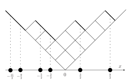
Figure 7: The Young diagram and the Maya diagram for $\mu=(5,3,1,1)$

A plane partition $\pi$ is an array of non-negative integers satisfying $\pi_{ij}\geq\pi_{i+1j}$ and $\pi_{ij}\geq\pi_{ij+1}$ for all $i,j\geq 1$. Plane partitions are identified with the three-dimensional Young diagrams. The three-dimensional diagram $\pi$ is a set of unit cubes such that $\pi_{ij}$ cubes are stacked vertically on each $(i,j)$-element of $\pi$. See Figure 8.

\psfrag{pi0}{$\pi(0)$}\psfrag{m}{m}\psfrag{0}{0}\psfrag{pi}{$\pi_{ij}$}\psfrag{i}{$i$}\psfrag{j}{$j$}\includegraphics{pl.eps}

Figure 8: The three-dimensional Young diagram and its diagonal slices

The size of $\pi$ is defined by $|\pi|=\sum_{i,j\geq 1}\pi_{ij}$, which is the total number of cubes of the diagram. Diagonal slices of $\pi$ become partitions. Let $\pi(m)$ denote the partition along the $m$-th diagonal slice. In particular $\pi(0)$ is the main diagonal partition. See also Figure 8. The series of partitions $\pi(m)$ satisfies the condition

$$\cdots\prec\pi(-2)\prec\pi(-1)\prec\pi(0)\succ\pi(1)\succ\pi(2)\succ\cdots,$$ (4.1)

where $\mu\succ\nu$ means the following interlace relation between two partitions $\mu$ and $\nu$.

$$\mu\succ\nu~{}~{}~{}\Longleftrightarrow~{}~{}~{}\mu_{1}\geq\nu_{1}\geq\mu_{2}\geq\nu_{2}\geq\mu_{3}\geq\cdots.$$ (4.2)

We first consider a statistical model of plane partitions defined by the following partition function.

$$Z(q,Q) \equiv \sum_{\pi}\,q^{|\pi|}\,Q^{|\pi(0)|}\,,$$ (4.3)

where $q$ and $Q$ are indeterminate. The Boltzmann weight consists of two parts. The first contribution comes from the energy of plane partitions, and the second contribution is a chemical potential for the main diagonal partitions.

The condition (4.1) suggests that plane partitions are certain evolutions of partitions by the discretized time $m$. This leads to a hamiltonian formulation for the statistical model. In particular, the transfer matrix approach developed in [19] express the partition function (4.3) in terms of two-dimensional conformal field theory. Let us recall that partitions can be mapped to the Fock space of two-dimensional free fermions by

$$|\mu;p\rangle=\Bigl{(}\prod\limits_{i=1}^{l(\mu)}\psi_{-x_{i}(\mu)-p}\Bigr{)}\Bigl{(}\prod\limits_{i=1}^{l(\mu)}\psi^{*}_{-i+\frac{1}{2}+p}\Bigr{)}|\emptyset;p\rangle\,,$$ (4.4)

where $l(\mu)$ denotes the length of $\mu$, that is, the number of the non-zero $\mu_{i}$, and the state $|\emptyset;p\rangle$ is the ground state for the charge $p$ sector. See appendix for details on the free fermion system. Combinations of partitions with the $U(1)$ charges are called charged partitions. Such a charged partition is denoted by $(\mu,p)$, where $\mu$ is a partition and $p$ is the $U(1)$ charge. To describe the transfer matrix, it is convenient to introduce vertex operators

$$\Gamma_{+}(z) \equiv \exp\Bigl{(}\sum\limits_{k=1}^{\infty}\frac{1}{k}z^{k}J_{k}\Bigr{)}\,,$$

$$\Gamma_{-}(z) \equiv \exp\Bigl{(}\sum\limits_{k=1}^{\infty}\frac{1}{k}z^{-k}J_{-k}\Bigr{)}\,.$$ (4.5)

where $J_{k}$ are the modes of the $U(1)$ current. These operators satisfy the following properties.

$$\langle\mu;p|\Gamma_{+}(z)|\lambda;p\rangle = \left\{\begin{array}[]{cc}z^{-|\mu|+|\lambda|}&\mbox{$\mu\prec\lambda$}\\ 0&\mbox{otherwise}\,.\end{array}\right.$$ (4.8)

$$\langle\mu;p|\Gamma_{-}(z)|\lambda;p\rangle = \left\{\begin{array}[]{cc}z^{-|\mu|+|\lambda|}&\mbox{$\mu\succ\lambda$}\\ 0&\mbox{otherwise}\,.\end{array}\right.$$ (4.11)

By comparing (4.11) with (4.1), we see that these operators can provide a description of the evolutions of partitions. The evolution at a negative time $m$ is given by $\Gamma_{+}(q^{-(m+\frac{1}{2})})$, while the evolution at a nonnegative time $m$ is by $\Gamma_{-}(q^{-(m+\frac{1}{2})})$. The partition function has the following expression by using the vertex operators.

$$Z(q,Q)=\langle\emptyset;0|\Bigl{(}\prod\limits_{m=-\infty}^{-1}\Gamma_{+}(q^{-(m+\frac{1}{2})})\Bigr{)}\,Q^{L_{0}}\,\Bigl{(}\prod\limits_{m=0}^{\infty}\Gamma_{-}(q^{-(m+\frac{1}{2})})\Bigr{)}|\emptyset;0\rangle\,.$$ (4.12)

We can interpret the random plane partitions as a $q$-deformation of random partitions. It may be seen by rewriting (4.3) as

$$Z(q,Q)=\sum_{\mu}\,Q^{|\mu|}\,\Bigl{(}\sum_{\pi(0)=\mu}\,q^{|\pi|}\Bigr{)}\,.$$ (4.13)

The partitions $\mu$ are thought as the ensemble of the model by summing first over plane partitions whose main diagonal partitions are $\mu$. In the transfer matrix description this is obtained by factorizing the amplitude (4.12) at $m=0$. The factorization by using the charged partition states (4.4) gives rise to

$$Z(q,Q)=\sum_{\mu}Q^{|\mu|}s_{\mu}(q^{\frac{1}{2}},q^{\frac{3}{2}},\cdots)^{2},$$ (4.14)

where $s_{\mu}(q^{\frac{1}{2}},q^{\frac{3}{2}},\cdots)$ is the Schur function $s_{\mu}(x_{1},x_{2},\cdots)$ specialized at $x_{i}=q^{i-\frac{1}{2}}$ [20].

4.2 Random plane partitions and supersymmetric gauge theories

The Fock representation of a single complex fermion has [21] an alternative realization that is obtained by exploiting $N$ component complex fermions $\psi^{(r)}(z)$, $\psi^{*(s)}(z)$ according to the identification.

$$\psi_{k}^{(r)}=\psi_{N(k-\xi_{r})}\,,\hskip 22.76219pt\psi_{l}^{(s)*}=\psi_{N(l+\xi_{s})}\,,$$ (4.15)

where $k,l\in\mathbb{Z}+\frac{1}{2}$ and $r,s=1,2,\ldots,N$. This allows us to express a charged partition $(\mu,p)$ uniquely by means of $N$ charged partitions $(\lambda^{(r)},p_{r})$ and vice versa, through the realizations of the charged partition state.

$$|\mu;p\rangle=\bigotimes_{r=1}^{N}|\lambda^{(r)};p_{r}\rangle_{(r)}\,.$$ (4.16)

The equality can be read in terms of the characteristic functions (A.8) for charged partitions as follows.

$$P_{\mu,\,p}(t)=\sum_{r=1}^{N}e^{N\xi_{r}t}P_{\lambda^{(r)},\,p_{r}}(Nt)\,.$$ (4.17)

By applying the method of power-sums [22] one can deduce the following information from (4.17).

$$p = \sum\limits_{r=1}^{N}p_{r}\,,$$ (4.18)

$$|\mu| = N\sum\limits_{r=1}^{N}|\lambda^{(r)}|+\frac{N}{2}\sum\limits_{r=1}^{N}p_{r}^{2}+\sum\limits_{r=1}^{N}rp_{r}\,,$$ (4.19)

$$\kappa(\mu) = N^{2}\sum\limits_{r=1}^{N}\kappa(\lambda^{(r)})+2N^{2}\sum\limits_{r=1}^{N}\widetilde{p}_{r}|\lambda^{(r)}|+\frac{N^{2}}{3}\sum\limits_{r=1}^{N}\widetilde{p}_{r}^{3}\,,$$ (4.20)

where $\kappa(\mu)$ measures asymmetry of a partition and is defined by $2\kappa(\mu)\equiv\sum\limits_{i\geq 1}\mu_{i}^{2}-\sum\limits_{i\geq 1}\,^{t}\mu^{2}_{i}$. Here ${}^{t}\mu$ denotes the partition conjugate to $\mu$, which is obtained by flipping the Young diagram $\mu$ over its main diagonal.

The factorization (4.13) or (4.14) can be also expressed in terms of $N$ charged partitions, by using (4.16). Let us factor the partition function into

$$Z(q,Q)=\sum_{p_{r}}Z_{SU(N)}(p_{r};q,Q)\,,$$ (4.21)

where the $U(1)$ charges $p_{r}$ automatically satisfy the $SU(N)$ condition (3.36), due to the charge conservation (4.18). We have included the summation over partitions $\lambda^{(r)}$ implicitly in $Z_{SU(N)}(p_{r};q,Q)$.

The factorization (4.21) turns to be a bridge between the random plane partitions and supersymmetric gauge theories. We identify the parameters $q,Q$ and $p_{r}$ with the gauge theory parameters as follows.

$$q=e^{-\frac{2}{N}R\hbar},\hskip 11.38109ptQ=(2R\Lambda)^{2},\hskip 11.38109pt\widetilde{p}_{r}=a_{r}/\hbar\,.$$ (4.22)

It is shown in [8] that the above identification leads to

$$Z_{SU(N)}(p_{r};q,Q)=Z_{5d\,\mbox{\scriptsize{SYM}}}(a_{r};\Lambda,R,\hbar)\,,$$ (4.23)

where the RHS is the exact partition function [7] for five-dimensional $\mathcal{N}=1$ supersymmetric $SU(N)$ Yang-Mills plus the Chern-Simons term having the coupling constant equal to $N$.

Since the K$\ddot{\mbox{a}}$hler gravity on local $SU(N)$ geometry has the relation to the perturbative dynamics of the gauge theory, we take a closer look of the perturbative contribution in (4.23). A charged ground partition is a charged partition determined by a set of $N$ charged empty partitions $(\emptyset,p_{r})$ by using (4.16). The neutral ground partition is simply called ground partition and is denoted by $\mu_{\mbox{\tiny{GP}}}(p_{r})$. A set $\mathcal{M}(p_{r})$ is a set of plane partitions such that

$$\mathcal{M}(p_{r})\equiv\Bigl{\{}\pi\,\,;\,\pi(0)=\mu_{\mbox{\tiny{GP}}}(p_{r})\Bigr{\}}\,.$$ (4.24)

The perturbative contribution can be described [8] by random plane partitions restricted within $\mathcal{M}(p_{r})$.

$$Z_{SU(N)}^{pert}(p_{r};q,Q)=Q^{\left|\mu_{\mbox{\tiny{GP}}}(p_{r})\right|}\sum_{\,\,\pi\in\mathcal{M}(p_{r})}q^{|\pi|}\,.$$ (4.25)

This turns out to be written by using the Schur function as follows.

$$Z_{SU(N)}^{pert}(p_{r};q,Q)=Q^{\left|\mu_{\mbox{\tiny{GP}}}(p_{r})\right|}s_{\mu_{\mbox{\tiny{GP}}}(p_{r})}(q^{\frac{1}{2}},\,q^{\frac{3}{2}},\,\cdots)^{2}\,.$$ (4.26)

4.3 Ground plane partition and quantum foam of local $SU(N)$ geometry

We consider the ground state of the statistical model (4.25). Such a ground state is called ground plane partition and is denoted by $\pi_{\mbox{\tiny{GPP}}}(p_{r})$. It is a plane partition in $\mathcal{M}(p_{r})$ which satisfies

$$|\pi_{\mbox{\tiny{GPP}}}(p_{r})|\,\leq\,|\mu|\hskip 17.07164pt\mbox{for}\hskip 8.53581pt\forall\mu\in\mathcal{M}(p_{r})\,.$$ (4.27)

The above condition uniquely determines the ground plane partition. We regard plane partitions as the series of partitions. A series of partitions $\pi(m)$ gives an element of $\mathcal{M}(p_{r})$ only when it evolves from/to $\pi(0)=\mu_{\mbox{\tiny{GP}}}(p_{r})$ satisfying the interlace condition (4.1) at each discrete time. Since the Boltzmann weight is written as $|\pi|=\sum\limits_{m}|\pi(m)|$, the least action can be realized by the series that minimizes $|\pi(m)|$ at each $m$ from among partitions allowed by the interlace condition. The minimizations starting at $m=\pm 1$ determine the series recursively. See Figure 9. These give rise to

$$\pi_{\mbox{\tiny{GPP}}}(p_{r})(m)_{i}=\mu_{\mbox{\tiny{GP}}}(p_{r})_{i+|m|}\,.$$ (4.28)

We note that the ground plane partition is actually the ground state of the model (4.23) and is regarded as a classical trajectory of the hamiltonian dynamics.

\psfrag{a11}{$\pi_{11}$}\psfrag{a12}{$\pi_{12}$}\psfrag{a13}{$\pi_{13}$}\psfrag{a14}{$\pi_{14}$}\psfrag{a15}{$\pi_{15}$}\psfrag{a21}{$\pi_{21}$}\psfrag{a22}{$\pi_{22}$}\psfrag{a23}{$\pi_{23}$}\psfrag{a24}{$\pi_{24}$}\psfrag{a25}{$\pi_{25}$}\psfrag{a31}{$\pi_{31}$}\psfrag{a32}{$\pi_{32}$}\psfrag{a33}{$\pi_{33}$}\psfrag{a34}{$\pi_{34}$}\psfrag{a35}{$\pi_{35}$}\psfrag{a41}{$\pi_{41}$}\psfrag{a42}{$\pi_{42}$}\psfrag{a43}{$\pi_{43}$}\psfrag{a44}{$\pi_{44}$}\psfrag{a45}{$\pi_{45}$}\psfrag{a51}{$\pi_{51}$}\psfrag{a52}{$\pi_{52}$}\psfrag{a53}{$\pi_{53}$}\psfrag{a54}{$\pi_{54}$}\psfrag{a55}{$\pi_{55}$}\includegraphics{GPP.eps}

Figure 9: The minimizations determine the ground plane partition by equating $\pi_{ij}$ that are connected by the dashed lines.

4.3.1 Perturbative gauge theory prepotential from ground plane partition

We order the $U(1)$ charges such that $p_{1}\leq p_{2}\leq\cdots\leq p_{N}$. We first describe the ground partition explicitly. Use of $T_{k}$ becomes convenient rather than $p_{r}$ in the description. These were the quantized K$\ddot{\mbox{a}}$hler parameters in the previous section and are related with the $U(1)$ charges by (3.35). The ground partition becomes a partition of length $\sum\limits_{r=1}^{N-1}rT_{r}$ and is given by

$$\mu_{\mbox{\tiny{GP}}}(p_{r})_{r(m-1)+n+\sum\limits_{k=1}^{r-1}kT_{k}}=-(N-r)(m-1)+\sum\limits_{k=r}^{N-1}(N-k)T_{k}\,,$$ (4.29)

where $1\leq r\leq N-1,\,1\leq m\leq T_{r}$ and $1\leq n\leq r$. The corresponding Young diagram is depicted in Figure 10. Note that the size of ground partition can be read from (4.19) and is expressed by means of $T_{k}$ as follows.

$$|\mu_{\mbox{\tiny{GP}}}(p_{r})| = N\sum_{k=1}^{N-1}\frac{1}{2k(k+1)}\Bigl{(}\sum_{i=1}^{k}iT_{i}\Bigr{)}^{2}+\sum_{k=1}^{N-1}\frac{k(N-k)}{2}T_{k}\,.$$ (4.30)

\psfrag{v1}{$(N-1)T_{1}$}\psfrag{v2}{$(N-2)T_{2}$}\psfrag{v3}{$\vdots$}\psfrag{vN}{$T_{N-1}$}\psfrag{h1}{$T_{1}$}\psfrag{h2}{$2T_{2}$}\psfrag{h3}{$\cdots$}\psfrag{hN}{$(N-1)T_{N-1}$}\includegraphics{muGP.eps}

Figure 10: The Young diagram $\mu_{\mbox{\tiny{GP}}}(p_{r})$

Let us compute the size of ground plane partition. It follows from (4.28) that the size is represented as

$$|\pi_{\mbox{\tiny{GPP}}}(p_{r})| = \sum_{i\geq 1}~{}^{t}\mu_{\mbox{\tiny{GP}}}(p_{r})_{i}^{2}\,.$$ (4.31)

The RHS can be computed by using (4.29) and we obtain

$$|\pi_{\mbox{\tiny{GPP}}}(p_{r})|=N\sum_{k=1}^{N-1}\frac{1}{3k(k+1)}\Bigl{(}\sum_{i=1}^{k}iT_{i}\Bigr{)}^{3}+\sum_{k=1}^{N-1}\frac{1}{2}\Bigl{(}\sum_{i=1}^{k}iT_{i}\Bigr{)}^{2}+\sum_{k=1}^{N-1}\frac{k^{2}(N-k)}{6}T_{k}\,.$$ (4.32)

We consider the Boltzmann weight for ground plane partition. We first note that, by combining the identifications (3.37) and (4.22), the parameters $q$ and $Q$ in the statistical model have the following expression.

$$q=e^{-g_{st}/N},\hskip 14.22636ptQ=q^{T_{N}}\,.$$ (4.33)

This allows us to write the Boltzmann weight as

$$q^{|\pi|}\,Q^{|\pi(0)|}=q^{|\pi|+T_{N}|\pi(0)|}\,.$$ (4.34)

The exponent for ground plane partition is obtained from (4.30) and (4.32). By comparing with (3.34) we find

$$|\pi_{\mbox{\tiny{GPP}}}(p_{r})|+T_{N}|\mu_{\mbox{\tiny{GP}}}(p_{r})|=N\times\mbox{Vol}(\mathcal{P}^{c}(D))+O(T^{2})\,.$$ (4.35)

Therefore the ground state energy gives rise to the gauge theory prepotential (3.41).

$$-\ln\,q^{|\pi_{\mbox{\tiny{GPP}}}(p_{r})|}\,Q^{|\mu_{\mbox{\tiny{GP}}}(p_{r})|}=\frac{1}{\hbar^{2}}\Bigl{\{}\mathcal{F}^{pert}_{\mbox{{\scriptsize 5dSYM}}}(a,\,\Lambda,\,R)+O(\hbar)\Bigr{\}}\,.$$ (4.36)

Let us make a few comments. The first is about (4.34). This expression for the Boltzmann weight suggests that, in the hamiltonian approach the potential term $Q^{|\pi(0)|}$ might as well be absorbed as a jump of discrete time. Note that the transfer matrix in (4.12) can be replaced with the following one.

$$\prod\limits_{m=-\infty}^{-1}\Gamma_{+}(q^{-(m-\frac{T_{N}}{2}+\frac{1}{2})})\cdot 1^{T_{N}}\cdot\prod\limits_{m=0}^{\infty}\Gamma_{-}(q^{-(m+\frac{T_{N}}{2}+\frac{1}{2})})\,.$$ (4.37)

This implies that the potential term delays or advances the discrete time by the amount of $T_{N}$. The second is on (4.35). When the $U(1)$ charges are very large, we can approximate the ground plane partition, regarding as the three-dimensional Young diagram, to a three-dimensional solid. See Figure 11(a). The asymptotics of the ground partition is shaded in the figure. The size of ground plane partition in (4.35) is estimated as its volume. This consideration is generalized to the contribution of ground partition in (4.35), by thinking about another solid (Figure 11(b)). By taking the first comment into account, we can imagine a new solid obtained from the two by cut and paste. Figure 11(c). Eq.(4.35) says that the volume of the last solid, measured by letting the unit cube in the plane partitions be one, is equal to $N$ times the volume of $\mathcal{P}^{c}(D)$, measured by letting the minimal volume in the K$\ddot{\mbox{a}}$hler gravity be one.

\psfrag{(a)}{$(a)$}\includegraphics[scale={.6}]{piGPP.eps}	\psfrag{(b)}{$(b)$}\psfrag{TN}{$T_{N}$}\includegraphics[scale={.6}]{piGPP2.eps}
\psfrag{(c)}{$(c)$}\includegraphics[scale={.6}]{piGPP3.eps}

Figure 11: Three-dimensional solids obtained from the ground plane partition

4.3.2 Ground plane partition and quantum foam

Three-dimensional Young diagrams are interpreted as the sets of lattice points, by regarding each cube as a lattice point. Let $\mbox{Supp}(\pi)$ denote the set of $(i,j)$ that satisfy $\pi_{ij}\neq 0$. A plane partition $\pi$ is identified with

$$\pi=\Bigl{\{}(i,j,k)\in\mathbb{Z}^{\oplus 3}\,;\,(i,j)\in\mbox{Supp}(\pi),\,1\leq k\leq\pi_{ij}\Bigr{\}}\,.$$ (4.38)

We will realize the lattice as a degree two sublattice of $L$

$$M^{\mbox{\tiny{PP}}}\equiv\mathbb{Z}(e_{x}-e_{y})+\mathbb{Z}(e_{x}+e_{y})+\mathbb{Z}e_{z}\,,$$ (4.39)

by the mapping

$$(i,j,k)\,\longmapsto\,\left\{\begin{array}[]{cc}(i-1)e_{x}+(2j-i-1)e_{y}+(k-1)e_{z}&\hskip 11.38109ptj-i\geq 1\\ (i-1)e_{x}+(j-1)e_{y}+(k-1)e_{z}&\hskip 11.38109ptj=i\\ (2i-j-1)e_{x}+(j-1)e_{y}+(k-1)e_{z}&\hskip 11.38109ptj-i\leq-1\,.\end{array}\right.$$ (4.43)

See Figure 12.

\psfrag{ex}{$e_{x}$}\psfrag{ey}{$e_{y}$}\includegraphics{Lattice.eps}

Figure 12: The sublattice $M^{\mbox{\tiny{PP}}}$ consists of the bullets in the lattice $L$.

We may divide the lattice points into the subsets $\pi^{(+)},\pi^{(-)}$ and $\pi^{(0)}$ by regarding plane partitions as the series of partitions. They respectively consist of lattice points that come from the partitions $\pi(m)$ at $m\geq 1,m\leq-1$ and $m=0$. Let $\widehat{\pi}^{(+)}(T_{N}),\widehat{\pi}^{(-)}(T_{N})$ and $\widehat{\pi}^{(0)}(T_{N})$ denote sets of lattice points in $L$ that are determined from $\pi^{(+)},\pi^{(-)}$ and $\pi^{(0)}$ by

$$\widehat{\pi}^{(+)}(T_{N}) = \pi^{(+)}+T_{N}e_{y}\,,$$

$$\widehat{\pi}^{(-)}(T_{N}) = \pi^{(-)}+T_{N}e_{x}\,,$$ (4.44)

$$\widehat{\pi}^{(0)}(T_{N}) = \bigcup_{k=0}^{T_{N}}\Bigl{\{}\pi^{(0)}+T_{N}e_{x}+k(-e_{x}+e_{y})\Bigr{\}}\,.$$

The union of the above, which we call $\widehat{\pi}(T_{N})$, clearly incorporates the jumping effect. In particular, it satisfies $|\widehat{\pi}(T_{N})|=|\pi|+T_{N}|\pi(0)|$. Note that translations involving $T_{N}e_{x}$ and $T_{N}e_{y}$ in (4.44) make $\widehat{\pi}(T_{N})\subset M^{\mbox{\tiny{PP}}}$ or $\widehat{\pi}(T_{N})\subset M^{\mbox{\tiny{PP}}}+e_{x}$.

Let $\widehat{\pi}_{\mbox{\tiny{GPP}}}(p_{r};T_{N})$ be the set of lattice points in $L$ that is obtained from $\pi_{\mbox{\tiny{GPP}}}(p_{r})$ as above. It can be observed that $\widehat{\pi}_{\mbox{\tiny{GPP}}}(p_{r};T_{N})$ becomes approximately $P_{(0,\cdots,0,T_{N})}\setminus P_{T}$ when $T$ are very large. Actually we find

$$\widehat{\pi}_{\mbox{\tiny{GPP}}}(p_{r};T_{N})\cap\iota(M) = \bigl{(}P_{(0,\cdots,0,T_{N})}\setminus P_{T}\bigr{)}\cap\iota(M)$$ (4.45)

$$= \iota(\mathcal{P}^{c}(D)\cap M)\,.$$

Note that $\iota(M)$ can be considered as a degree $N$ sublattice of $M^{\mbox{\tiny{PP}}}$. This implies that each gravitational quantum of the $SU(N)$ geometry consists of $N$ cubes of plane partitions. This also explains the factor $N$ which appears in (4.35).

4.4 Generalized models of random plane partitions

In order to relate random plane partitions with local $SU(N)$ geometries having other framings or five-dimensional gauge theories with the Chern-Simons terms taking other coupling constants, a slight modification of the model (4.3) is required. The relevant model is defined by

$$Z(q,Q\,;\,\widetilde{k}_{\mbox{\tiny{C.S.}}})\equiv\sum\limits_{\pi}q^{|\pi|+\frac{\widetilde{k}_{\mbox{\tiny{C.S.}}}}{2N}\kappa(\pi(0))}\,Q^{|\pi(0)|}\,.$$ (4.46)

By repeating the previous argument and also taking account of (4.20), one can find particularly

$$-\ln\,q^{|\pi_{\mbox{\tiny{GPP}}}(p_{r})|+\frac{\widetilde{k}_{\mbox{\tiny{C.S.}}}}{2N}\kappa(\mu_{\mbox{\tiny{GP}}}(p_{r}))}\,Q^{|\mu_{\mbox{\tiny{GP}}}(p_{r})|}=\frac{1}{\hbar^{2}}\Bigl{\{}\mathcal{F}^{pert}_{\mbox{{\scriptsize 5dSYM}}}(a,\,\Lambda,\,R)+O(\hbar)\Bigr{\}}\,,$$ (4.47)

where the gauge theory prepotential is (3.78). This describes the case of the Chern-Simons term taking the coupling constant $k_{\mbox{\tiny{C.S.}}}$.

The transfer matrix for the above model naturally involves the charges of higher spin currents of $W_{1+\infty}$ algebra [23] by (A.9).

$$Z(q,Q\,;\,\widetilde{k}_{\mbox{\tiny{C.S.}}})=\langle\emptyset;0|\Bigl{(}\prod\limits_{m=-\infty}^{-1}\Gamma_{+}(q^{-(m+\frac{1}{2})})\Bigr{)}\,Q^{L_{0}}\,q^{\frac{\widetilde{k}_{\mbox{\tiny{C.S.}}}}{2N}W^{3}_{0}}\,\Bigl{(}\prod\limits_{m=0}^{\infty}\Gamma_{-}(q^{-(m+\frac{1}{2})})\Bigr{)}|\emptyset;0\rangle\,,$$ (4.48)

where $L_{0}=W^{2}_{0}$ and $W^{3}_{0}$ are respectively the charges of the spin two and spin three currents (A.5). This seems to suggest some physical/geometrical importance in a further generalization of the statistical model such as

$$Z(q\,;\,s_{2},\,s_{3},\,\ldots)=\langle\emptyset;0|\Bigl{(}\prod\limits_{m=-\infty}^{-1}\Gamma_{+}(q^{-(m+\frac{1}{2})})\Bigr{)}\,q^{\sum\limits_{n=2}^{\infty}s_{n}W_{0}^{n}}\,\Bigl{(}\prod\limits_{m=0}^{\infty}\Gamma_{-}(q^{-(m+\frac{1}{2})})\Bigr{)}|\emptyset;0\rangle\,.$$ (4.49)

Appendix A $2d$ Free Fermions, Partitions and $W_{1+\infty}$-Algebra

Let $\psi(z)=\sum\limits_{r\in\mathbb{Z}+\frac{1}{2}}\psi_{r}z^{-r-\frac{1}{2}}$ and $\psi^{*}(z)=\sum\limits_{s\in\mathbb{Z}+\frac{1}{2}}\psi^{*}_{s}z^{-s-\frac{1}{2}}$ be complex fermions with the anti-commutation relations $\left\{\psi_{r},\psi_{s}^{*}\right\}=\delta_{r+s\,,\,0}$. In the fermion system, ground state for the charge $p$ sector is defined by the conditions

$$\psi_{r}|\emptyset;p\rangle=0 \mbox{for $r>-p$}\,,$$

$$\psi_{s}^{*}|\emptyset;p\rangle=0 \mbox{for $s>p$}\,.$$ (A.1)

For each partition $\mu$, the corresponding charged state $|\mu;\,p\rangle$ is built on the ground state as described in (4.4).

$W_{1+\infty}$ algebra is obtained [23] from the algebra of psedo-differential operators by its central extension. Let us put $D=z\frac{d}{dz}$. Consider

$$W[z^{n}D^{k}]\equiv\oint\frac{dz}{2\pi i}:\psi(z)z^{n}D^{k}\psi^{*}(z):\,,$$ (A.2)

where $:\hskip 5.69054pt:$ denotes the standard normal ordering and is prescribed by

$$:\,\psi(z)\psi^{*}(w):\hskip 5.69054pt=\psi(z)\psi^{*}(w)-\frac{1}{z-w}\,.$$ (A.3)

These operators constitute the algebra.

$$\Bigl{[}W[z^{n_{1}}D^{k_{1}}]\,,\,W[z^{n_{2}}D^{k_{2}}]\Bigr{]} = W\bigl{[}z^{n_{1}+n_{2}}\bigl{\{}(D+n_{2})^{k_{1}}D^{k_{2}}-D^{k_{1}}(D+n_{1})^{k_{2}}\bigr{\}}\bigr{]}$$ (A.4)

$$+\Psi(z^{n_{1}}D^{k_{1}},z^{n_{2}}D^{k_{2}})\,\,,$$

where $\Psi$ denotes the central extension. It becomes possible [24] to choose a basis for the algebra so that central charges between different spin operators vanish. In such a basis the lower spin operators have the following form.

$$W^{1}_{n} = W[z^{n}]\,,$$

$$W^{2}_{n} = -W[z^{n}D]-\frac{n+1}{2}W[z^{n}]\,,$$ (A.5)

$$W^{3}_{n} = W[z^{n}D^{2}]+(n+1)W[z^{n}D]+\frac{(n+1)(n+2)}{6}W[z^{n}]\,.$$

Among them, $J_{n}\equiv W^{1}_{n}$ and $L_{n}\equiv W^{2}_{n}$ constitute the Virasoro subalgebra.

$$\left[J_{k}\,,\,J_{k^{\prime}}\right] = k\delta_{k+k^{\prime},\,0}\,\,,$$

$$\left[L_{m}\,,\,J_{k}\right] = -kJ_{k+n}\,\,,$$ (A.6)

$$\left[L_{m}\,,\,L_{n}\right] = (m-n)L_{m+n}+\frac{n}{12}(n^{2}-1)\delta_{n+m\,,\,0}\,\,.$$

Charged partition states (4.4) become simultaneous eigenstates of infinitely many charges in $W_{1+\infty}$ algebra.

$$W\bigl{[}e^{-t(D+\frac{1}{2})}\bigr{]}\,|\mu;\,p\rangle=\Bigl{(}P_{\mu,\,p}(t)-P_{\emptyset,\,p}(t)+e^{\frac{t}{2}}\frac{e^{pt}-1}{e^{t}-1}\Bigr{)}|\mu;\,p\rangle\,,$$ (A.7)

where the operator in the LHS is a generating function of the charges, and $P_{\mu,\,p}(t)$ in the RHS denotes the characteristic function [22] defined by

$$P_{\mu,\,p}(t)=\sum\limits_{i=1}^{\infty}e^{(p+\mu_{i}-i+\frac{1}{2})t}\,.$$ (A.8)

For the lower spin operators (A.5), the above gives rise to

$$W^{1}_{0}\,|\mu;\,p\rangle = p\,|\mu;\,p\rangle\,,$$

$$W^{2}_{0}\,|\mu;\,p\rangle = \Bigl{(}|\mu|+\frac{p^{2}}{2}\Bigr{)}\,|\mu;\,p\rangle\,,$$ (A.9)

$$W^{3}_{0}\,|\mu;\,p\rangle = \Bigl{(}\kappa(\mu)+\frac{p^{3}}{3}\Bigr{)}\,|\mu;\,p\rangle\,.$$

Acknowledgements

We thank to T. Kimura for a useful discussion on toric geometries. T.N. is supported in part by Grant-in-Aid for Scientific Research 15540273.

References

• [1] A. Okounkov, N. Reshetikhin and C. Vafa, “Quantum Calabi-Yau and Classical Crystals,” hep-th/0309208.
• [2] A. Iqbal, N. Nekrasov, A. Okounkov and C. Vafa, “Quantum Foam and Topological Strings,” hep-th/0312022.
• [3] M. Bershadsky and V. Sadov, “Theory of K$\ddot{\mbox{a}}$hler Gravity,” Int. J. Mod. Phys. A11 (1196) 4689, hep-th/9410011
• [4] E. Witten, “Two-dimensional gravity and intersection theory on moduli space,” Surveys Diff. Geom. 1 (1991) 243.
• [5] A. Iqbal, “All Genus Topological String Amplitudes and 5-brane Webs as Feynman Diagrams,” hep-th/0207114.
M. Aganagic, A. Klemm, M. Marino and C. Vafa, “The Topological Vertex,” hep-th/0305132.
• [6] A. Iqbal and A.-K. Kashani-Poor, $SU(N)$ geometries and topological string amplitudes,” hep-th/0306032.
T. Eguchi and H. Kanno, “Topological strings and Nekrasov’s formulas,” JHEP 12 (2003) 006, hep-th/0310235.
• [7] N. A. Nekrasov, “Seiberg-Witten Prepotential from Instanton Counting,” Adv. Theor. Math. Phys. 7 (2004) 831, hep-th/0206161.
N. Nekrasov and A. Okounkov, “Seiberg-Witten Theory and Random Partitions,” hep-th/0306238.
• [8] T. Maeda, T. Nakatsu, K. Takasaki and T. Tamakoshi, “Five-Dimensional Supersymmetric Yang-Mills Theories and Random Plane Partitions,” JHEP 0503 (2005) 056, hep-th/0412327.
• [9] A. Klemm, W. Lerche, P. Mayr, C. Vafa and N. P. Warner, “Self-Dual Strings and N=2 Supersymmetric Field Theory,” Nucl. Phys. B477 (1996) 746, hep-th/9604034.
S. Katz, A. Klemm and C. Vafa, “Geometric Engineering of Quantum Field Theories,” Nucl. Phys. B497 (1997) 173, hep-th/9609239.
• [10] N. Woodhause, “Geometric Quantization,” Oxford Univ. Press, 1992.
S. Bates and A. Weinstein, “Lectures on the Geometry of Quantization,” Berkeley Mathematics Lecture Notes 8, AMS, 1991.
• [11] N. Seiberg, “Five Dimensional SUSY Field Theories, Non-Trivial Fixed Points and String Dynamics,” Phys. Lett. B388 (1996) 753, hep-th/9608111.
• [12] K. Intriligator, D. Morrison and N. Seiberg, “Five-Dimensional Supersymmetric Gauge Theories and Degenerations of Calabi-Yau Spaces,” Nucl. Phys. B497 (1997) 56, hep-th/9702198.
A. Iqbal and V. Kaplunovsky, “Quantum Deconstruction of a 5D SYM and its Moduli Space,” JHEP 0405 (2004) 013, hep-th/0212098.
• [13] T. Maeda, T. Nakatsu, K. Takasaki and T. Tamakoshi, “Free fermion and Seiberg-Witten differential in random plane partitions,” Nucl. Phys. B715 (2005) 275, hep-th/0412329.
• [14] W. Fulton, “Introduction to Toric Varieties,” Princeton University Press, 1993.
• [15] T. Oda, “Convex Bodies and Algebraic Geometry,” Springer-Verlag, 1988.
• [16] C. Vafa and E. Zaslow eds, “Mirror Symmetry,” Clay Mathematics Monographs 1, AMS, CMI, 2003.
• [17] E. Witten, Nucl. Phys. B311 (1988/89) 46.
• [18] J. Navarro-Salas and P. Navarro, “Virasoro Orbits, $\mbox{AdS}_{3}$ Quantum Gravity and Entropy,” JHEP 9905 (1999) 009, hep-th/9903248,
T. Nakatsu, H. Umetsu, N. Yokoi, “Three-Dimensional Black Holes and Liouville Field Theory,” Prog. Theor. Phys. 102 (1999) 867, hep-th/9903259.
• [19] A. Okounkov and N. Reshetikhin, “Correlation Function of Schur Process with Application to Local Geometry of a Random 3-Dimensional Young Diagram,” J. Amer. Math. Soc. 16 (2003) no.3 581, math.CO/0107056.
• [20] I. G. Macdonald, “Symmetric Functions and Hall Polynomials,” Clarendon Press, 1995.
• [21] M. Jimbo and T.Miwa, “Solitons and Infinite Dimensional Lie Algebras,” Publ. RIMS, Kyoto Univ., 19 (1983) 943.
• [22] S. Bloch and A. Okounkov, “The Character of the Infinite Wedge Representation,” alg-geom/9712009.
• [23] M. Sato and Y. Sato, $in$ Nonlinear Partial Differential Equations in Applied Science; Proc. U.S.-Japan Seminar, Tokyo, 1982; Lect. Notes in Num. Anal. 5 (1982) 259.
• [24] H. Awata, M. Fukuma, Y. Matsuo and S. Odake, “Representation theory of the $W_{1+\infty}$ algebra,” Prog. Theor. Phys. Suppl. 118 (1995) 343, hep-th/9408158.