RIKEN-TH-42

OU-HET-526/2005

hep-th/0505066

Aspects of Phase Transition
in Gauge-Higgs Unification at Finite Temperature

Nobuhito Maru^(a) , Kazunori Takenaga^(b)

^(a) Theoretical Physics Laboratory, RIKEN, Wako, Saitama 351-0198, Japan

^(b) Department of Physics, Osaka University, Toyonaka, Osaka 560-0043, Japan

We study the phase transition in gauge-Higgs unification at finite temperature. In particular, we obtain the strong first order electroweak phase transition for a simple matter content yielding the correct order of Higgs mass at zero temperature. Two stage phase transition is found for a particular matter content, which is the strong first order at each stage. We further study supersymmetric gauge models with the Scherk-Schwarz supersymmetry breaking. We again observe the first order electroweak phase transition and multi stage phase transition.

1 Introduction

There has been paid much attention to the scenario of gauge-Higgs unification [1][2] for the possibility to solve the gauge hierarchy problem without supersymmetry (SUSY). In this scenario, Higgs fields are regarded as extra components in the original gauge field. The higher dimensional local gauge invariance ensures that the Higgs field is strictly massless. If spatial coordinates are compactified, then the extra component gauge field behaves as the scalar field at low energies. And the scalar field can develop the vacuum expectation values (VEV) through the dynamics of the Wilson line phases, which is called as the Hosotani mechanism [3].

The dynamics of the Wilson line phases has been studied from various points of view [4]. In particular, an attempt to identify the Wilson line degrees of freedom with the Higgs scalar in the standard model (or in the minimal SUSY standard model) has been explored. Since the mass of the Higgs scalar in the gauge-Higgs unification is calculable, insensitive to the ultraviolet physics and is generated by quantum corrections through the Coleman-Weinberg mechanism [6], so that it is natural to expect that the Higgs mass is light, at most, the order of the gauge boson mass. The general analyses have been made in refs.[7][8] and pointed out that the Higgs mass can be as heavy as possible to satisfy the present experimental lower bound of the Higgs mass. The scenario is one of the promising possibility beyond the standard model even though there are many issues that should be studied such as the fermion mass hierarchy problem.

The dynamics of the Wilson line phases is essentially the Coleman-Weinberg mechanism, so that the transition at finite temperature is expected to be the first order [9]. In fact, the authors of ref.[10] extensively studied the nature of the phase transition of the gauge-Higgs unification at finite temperature and investigated the origin of the first order phase transition. They have explicitly demonstrated the first order phase transition in certain models [11] and shown that the lighter Higgs mass gives us the stronger first order phase transition. The strong first order phase transition is favored from a point of view of the scenario of the electroweak baryogenesis [12].

In this paper we study the gauge-Higgs unification at finite temperature in other models, including supersymmetric gauge models, which are different from the ones studied in ref.[10]. In our model, there is no need to introduce massive fields, and the matter content is very simple. We do not consider matter fields belonging to the higher dimensional representation under the gauge group except the adjoint one. In this matter content, the mass of the Higgs scalar can be consistent with the experimental lower bound. We obtain that the phase transition is the first order and find that the transition is so strong as to satisfy the necessary condition for the electroweak baryogenesis. We also observe the tendency that heavier the Higgs mass becomes, weaker the first order phase transition is. We calculate the critical temperature at which the two degenerate vacua appear and estimate how strong the phase transition is in our models.

We also find an interesting phenomena for a certain matter content even in the the gauge-Higgs unification at finite temperature. There are two stage phase transitions, which has also been observed in the four dimensional SUSY model at finite temperature [13]. In our model at the first critical temperature, the vacuum with the $SU(2)\times U(1)$ gauge symmetry is degenerate with that respecting the $U(1)^{\prime}\times U(1)$ gauge symmetry. Decreasing the temperature further, at the second critical temperature, the vacuum with the $U(1)^{\prime}\times U(1)$ gauge symmetry is degenerate with the vacuum with the $U(1)_{em}$ gauge symmetry. Both phase transitions are the first order at each phase transition. We also analyze the strength of the phase transition at each critical temperature.

We also study SUSY models with the Scherk-Schwarz SUSY breaking [14] at finite temperature. We again find the phase transition to be very strong first order, which is favored from the electroweak baryogenesis. The relevant quantity to measure the strength of the phase transition is also evaluated. We also find multi (four in our case) phase transition in the SUSY model with a particular matter content. Except for the first phase transition where the vacua with the $SU(2)\times U(1)$ gauge symmetry and the $U(1)_{em}$ gauge symmetry are degenerate at the critical temperature, all of these vacua respect the $U(1)_{em}$ gauge symmetry are degenerate in the rest of the three phase transitions.

In the next section, we investigate the behavior of the effective potential for the Wilson line phases at finite temperature in our model and show that the phase transition is the first order. Then, we estimate the critical temperature and the strength of the phase transition. The phase transition is found to be very strong and provides us an interesting possibility for the electroweak baryogenesis. In section $3$, we study the case of SUSY gauge models with the Scherk-Schwarz SUSY breaking and study the effective potential for the Wilson line phases at finite temperature. For a particular matter content, we find multi phase transition, four stages phase transitions in our case, in which the phase transition is the first order. The final section is devoted to conclusions and discussions.

2 Non supersymmetric gauge models

Let us consider gauge theory coupled with matter at finite temperature in $D$ dimensions, where one of the space coordinate is compactified on an orbifold, $S^{1}/Z_{2}$. The space time is regarded as an $S^{1}\times M^{D-2}\times S^{1}/Z_{2}$, where the Euclidean time direction $\tau$ is effectively compactified on a circle, $S^{1}$ whose periodicity is given by $\beta\equiv T^{-1}$, where $T$ stands for the temperature, the radius of the other $S^{1}$ and its coordinate are denoted by $R$ and $y$, respectively. We decompose the $D$ dimensional gauge field $A_{\hat{\mu}}(\hat{\mu}=0,1,D-1)$ as $A_{\hat{\mu}}=(A_{\tau},A_{\mu},A_{y})$.

When one studies the gauge theory on the space time with boundaries, one needs to specify boundary conditions of fields for the compactified direction. The boundary condition for the Euclidean time direction is determined by quantum statistics, so that one uniquely assigns the (anti-)periodic boundary condition for (fermions)bosons, while for the orbifold $S^{1}/Z_{2}$, we must specify the boundary condition on the two fixed points of the orbifold, $y=0$ and $y=\pi R$ in addition to the $S^{1}$ direction. We define that

$$A_{\hat{\mu}}(x,y+2\pi R) = UA_{\hat{\mu}}(x,y)\,U^{\dagger},$$ (1)

$$\pmatrix{A_{\mu}\cr A_{y}\cr}(x,z_{i}-y) = P_{i}\pmatrix{A_{\mu}\cr-A_{y}\cr}(x,z_{i}+y)\,P_{i}^{\dagger}\quad(i=0,1),$$ (2)

where $U^{\dagger}=U^{-1},P_{i}^{\dagger}=P_{i}=P_{i}^{-1}$ and $z_{0}=0,z_{1}=\pi R$. The minus sign for $A_{y}$ is needed to preserve the gauge invariance under these transformations. Since a transformation $\pi R+y\rightarrow\pi R-y$ must be the same as a transformation $\pi R+y\rightarrow-(\pi R+y)\rightarrow\pi R-y$, we obtain that

$$U=P_{1}P_{0}$$ (3)

Hereafter, we consider $P_{i}$ is more fundamental quantity than $U$.

The orbifolding boundary conditions $P_{i}$ determine the gauge symmetry breaking patterns at the tree level. In this paper, we start with an $SU(3)$ gauge group and choose $P_{0}=P_{1}=\mbox{diag.}(1,1,-1)$. Since the zero mode field for $A_{\mu}^{a}$ is given by the generators of $SU(3),\lambda^{a=1,2,3,8}$ commuting with $P_{0,1}$, the $SU(3)$ breaks down to the $SU(2)\times U(1)$ gauge group. We are interested in the gauge symmetry breaking patterns of $SU(2)\times U(1)$ at finite temperature after taking quantum corrections into account, that is, the phase transition through the dynamics of the Wilson line phases at finite temperature.

The Wilson line phases for the choice of $P_{0,1}=\mbox{diag}(1,1,-1)$ is given by the zero mode field $A_{y}^{b}$ associated with the $SU(3)$ generators, $\lambda^{b=4,5,6,7}$, which anticommutes with $P_{0,1}$. Then, the zero mode,

$$\Phi\equiv\sqrt{2\pi R}\pmatrix{A_{y}^{4}-iA_{y}^{5}\cr A_{y}^{6}-iA_{y}^{7}\cr}$$ (4)

transforms as an $SU(2)$ doublet, so that we can regard $\Phi$ as a Higgs doublet. We see that the degrees of freedom of the Higgs doublet is embedded in the zero mode part of $A_{y}$. This is the idea of the gauge-Higgs unification.

We paramerize $\langle A_{y}\rangle$, utilizing the $SU(2)\times U(1)$ degrees of freedom, as

$$\langle A_{y}\rangle={a\over{g_{4}R}}{\lambda^{6}\over 2}\equiv A_{y}^{6(0)}{\lambda^{6}\over 2}$$ (5)

where $g_{4}\equiv g/\sqrt{2\pi R}$ and $a$ is a real parameter. The parameter $a$ is related with the Wilson line phases,

$$W = {\cal P}\mbox{exp}\left(ig\oint_{S^{1}}dyA_{y}\right)=\pmatrix{1&0&0\cr 0&\cos(\pi a)&i\sin(\pi a)\cr 0&i\sin(\pi a)&\cos(\pi a)}\qquad(a~{}~{}\mbox{mod}~{}2)$$ (9)

$$= \left\{\begin{array}[]{lll}SU(2)\times U(1)&\mbox{for}&a=0,\\[2.84544pt] U(1)^{\prime}\times U(1)&\mbox{for}&a=1\\[2.84544pt] U(1)_{em}&\mbox{for}&\mbox{otherwise}\end{array}\right.$$

We observe that, depending on the values of $a$, the gauge symmetry breaking patterns are different, and in order to obtain the correct pattern of electroweak symmetry breaking, one needs the fractional values of $a$. As we will see later, the values of $a$ is determined dynamically through the dynamics of the Wilson line phases by minimizing the effective potential for the phase $a$.

Now, let us introduce fermions belonging to the adjoint (fundamental) representation under the gauge group $SU(3)$ and denote their flavor number by $N_{adj}^{(\pm)}(N_{fd}^{(\pm)})$, where the sign $(\pm)$ stands for the intrinsic parity defined in refs.[16][7]. Similarly, $N_{adj}^{(\pm)s}(N_{fd}^{(\pm)s})$ means the flavor number for bosons belonging to corresponding representations

Following the standard prescription [3], it is straightforward to calculate the zero temperature part of the effective potential for the Wilson line phase $a$ (corresponding to the background field (5)),

$$V_{eff}^{T=0}(a) = {\Gamma(D/2)\over{{\pi^{D/2}(2\pi R)^{D}}}}\sum_{n=1}^{\infty}{1\over n^{D}}$$

$$\times \Biggl{[}\left(-(D-2)+(r2^{[D/2]})N_{adj}^{(+)}-N_{adj}^{(+)s}\right)\left(\cos[2\pi na]+2\cos[\pi na]\right)$$

$$+ \left((r2^{[D/2]})N_{adj}^{(-)}-N_{adj}^{(-)s}\right)\left(\cos[2\pi n(a-{1\over 2})]+2\cos[\pi n(a-1)]\right)$$

$$+ \left((r2^{[D/2]})N_{fd}^{(+)}-2N_{fd}^{(+)s}\right)\cos[\pi na]+\left((r2^{[D/2]})N_{fd}^{(-)}-2N_{fd}^{(-)s}\right)\cos[\pi n(a-1)]\Biggr{]},$$

where we have assumed the adjoint scalar is real and $r$ is ${1\over 2}({1\over 4})$ for Majorana (Majorana-Weyl fermion). We have ignored the irrelevant $a$-independent terms in Eq.(LABEL:shiki7).

Let us briefly present the main results of the reference [7]. We set $D=5$, which is implicitly assumed throughout this paper. For the flavor number chosen as

$$N_{adj}^{(+)s} = 0,~{}~{}N_{adj}^{(-)s}=0,~{}~{}N_{adj}^{(+)}=2,~{}~{}N_{adj}^{(-)}=0,$$

$$N_{fd}^{(+)} = 0,~{}~{}N_{fd}^{(-)}=8,~{}~{}N_{fd}^{(+)s}=4,~{}~{}N_{fd}^{(-)s}=2,$$ (11)

the minimum of the effective potential (LABEL:shiki7) is dynamically determined to be $a_{0}\simeq 0.0583$, so that the $SU(2)\times U(1)$ correctly breaks down to $U(1)_{em}$. The Higgs mass, which is obtained by the second derivative of the effective potential evaluated at the minimum, is calculated as

$$m_{H}^{2}\equiv{{\partial^{2}V_{eff}^{T=0}}\over{\partial{A_{y}^{6(0)}}^{2}}}\Bigg{|}_{a=a_{0}}=(gR)^{2}{{\partial^{2}V_{eff}^{T=0}}\over{\partial a^{2}}}\Bigg{|}_{a=a_{0}}\simeq\left(g_{4}^{2}\times 129~{}~{}\mbox{GeV}\right)^{2}.$$ (12)

In the scenario of the gauge-Higgs unification, we notice an important relation,

$$\langle\Phi\rangle={a_{0}\over{g_{4}R}}=v\sim 246~{}\mbox{GeV},$$ (13)

which has been used in Eq.(12).

Let us now consider the finite temperature part and study the phase transition of the model with the matter content (11). Following the standard prescription of the finite temperature field theories [17][18], the finite temperature part of the effective potential is obtained as

$$V_{eff}^{T\neq 0}(a) = {{2\Gamma(D/2)}\over{{\pi^{D/2}(2\pi R)^{D}}}}\sum_{l=1}^{\infty}\sum_{n=1}^{\infty}{1\over{\left[(2\pi Rn)^{2}+l^{2}/T^{2}\right]^{D/2}}}$$ (14)

$$\times \Biggl{[}\left(-(D-2)+(r2^{[D/2]})N_{adj}^{(+)}(-1)^{l}-N_{adj}^{(+)s}\right)\left(\cos[2\pi na]+2\cos[\pi na]\right)$$

$$+ \left((r2^{[D/2]})N_{fd}^{(+)}(-1)^{l}-2N_{fd}^{(+)s}\right)\cos[\pi na]$$

$$+ \left((r2^{[D/2]})N_{adj}^{(-)}(-1)^{l}-N_{adj}^{(-)s}\right)\left(\cos[2\pi n(a-{1\over 2})]+2\cos[\pi n(a-1)]\right)$$

$$+ \left((r2^{[D/2]})N_{fd}^{(-)}(-1)^{l}-2N_{fd}^{(-)s}\right)\cos[\pi n(a-1)]\Biggr{]},$$

where we have ignored the irrelevant constant. The total effective potential we study is given by

$$V_{eff}(a)=V_{eff}^{T=0}(a)+V_{eff}^{T\neq 0}(a).$$ (15)

It is useful to introduce a dimensionless quantity $z\equiv RT$ for numerical studies. We also note that the total effective potential is invariant under $a\rightarrow-a$ and $a\rightarrow 2-a$, which implies that it is enough to consider the region given by $0\leq a\leq 1$.

For the matter content given by Eq.(11), we study the behavior of the effective potential with respect to the various values of $z$. Figure 1 tells us that the phase transition is the first order.

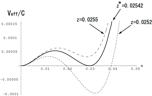
Figure 1: The behavior of the effective potential $V_{eff}(a)/C$ for a non-SUSY model with the matter content (11) is drawn with respect to $z\equiv RT$, where $C\equiv\Gamma(5/2)/\pi^{5/2}(2\pi R)^{5}$.

The critical temperature $T_{c}$, at which the two degenerate vacua appear, is numerically obtained as

$$z^{\star}\equiv RT_{c}\simeq 0.02542,$$ (16)

which gives the critical temperature

$$T_{c}\simeq{1\over R}\times 0.02542=\left({{g_{4}v}\over a_{0}}\right)\times 0.0254\simeq g_{4}\times 107.1~{}~{}\mbox{GeV}$$ (17)

where we have used the relation (13).

When one discusses the electroweak baryogenesis, the strength of the phase transition at finite temperature is crucial to satisfy the famous Zakharov’s conditions. Namely, the strong first order phases transition is required to decouple the sphaleron process to leave the generated baryon. The relevant quantity we examine is $v(T_{c})/T_{c}$ and should be larger than the unity, which is calculated as

$${v(T_{c})\over T_{c}}=\left({{a_{0}^{T_{c}}}\over{g_{4}R}}\right){1\over T_{c}}={1\over g_{4}}{{a_{0}^{T_{c}}}\over z^{*}}\simeq{1\over g_{4}}\times 1.19>1,$$ (18)

where $a_{0}^{T_{c}}$ is numerically calculated as

$$a_{0}^{T\neq 0}\simeq 0.0302.$$ (19)

The phase transition for the model with the matter content (11) through the dynamics of the Wilson line phases (the Hosotani mechanism) is found to be the strong first order as seen from Eq.(18) . Hence it may be possible to make use of this first order phase transition for the electroweak baryogenesis in the scenario of gauge-Higgs unification. One should observe that the light Higgs mass (small $g_{4}$) tends to make the phase transition stronger, which is consistent with the results obtained in ref.[10].

Next, we study the phase transition for other gauge symmetry breaking patterns determined by the values of $a$. This study is important to understand aspects and nature of the phase transition in the gauge-Higgs unification at finite temperature.

Let us choose the following extremely simplified matter content as

$$N_{adj}^{(+)s} = 0,~{}~{}N_{adj}^{(-)s}=0,~{}~{}N_{adj}^{(+)}=0,~{}~{}N_{adj}^{(-)}=0,$$

$$N_{fd}^{(+)} = 3,~{}~{}N_{fd}^{(-)}=0,~{}~{}N_{fd}^{(+)s}=0,~{}~{}N_{fd}^{(-)s}=0,$$ (20)

where the system corresponds to the gauge theory coupled to only the fundamental fermions. By numerical studies, we find the VEV, $a_{0}$ at the minimum of the effective potential (LABEL:shiki7) is given by

$$a_{0}=1.0.$$ (21)

From Eq.(9), we see that the unbroken gauge symmetry is $U(1)^{\prime}\times U(1)$, and the neutral gauge boson corresponding to the $Z$ boson in the standard model remains massless. The mass of the scalar that respects the $U(1)^{\prime}\times U(1)$ gauge symmetry is obtained as before,

$$m_{H}^{2}\simeq\left(g_{4}^{2}\times 24.03~{}~{}\mbox{GeV}\right)^{2}.$$ (22)

Taking the temperature effect into account, we can see again from Fig. 2 that the phase transition is the first order. The behavior of the effective potential is quite different from that of the previous example.

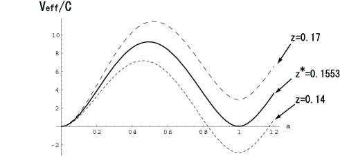
Figure 2: The behavior of the effective potential $V_{eff}(a)/C$ for a non-SUSY model with the matter content (20) is drawn with respect to $z\equiv RT$.

Contrary to the previous case, the local minimum for $T\geq T_{c}$ is always located as $a_{0}^{T\geq T_{c}}=1.0$. The critical temperature, at which the vacua with the $SU(2)\times U(1)$ gauge symmetry and the $U(1)^{\prime}\times U(1)$ gauge symmetry are degenerate, is given by

$$T_{c}\simeq{1\over R}\times 0.1553=\left({{g_{4}v}\over a_{0}}\right)\times 0.1553\simeq g_{4}\times 38.20~{}~{}\mbox{GeV}.$$ (23)

We calculate the relevant quantity to see how strong the phase transition is as

$${v(T_{c})\over T_{c}}=\left({{a_{0}^{T_{c}}}\over{g_{4}R}}\right){1\over T_{c}}={1\over g_{4}}{{a_{0}^{T_{c}}}\over z^{*}}\simeq{1\over g_{4}}\times 6.392>1.$$ (24)

We observe again the strong first order phase transition, and the mass of the scalar respecting the $U(1)^{\prime}\times U(1)$ gauge symmetry is very light, as shown in Eq.(22).

Let us finally consider the case where we introduce only the adjoint fermions instead of the fundamental one,

$$N_{adj}^{(+)s} = 0,~{}~{}N_{adj}^{(-)s}=0,~{}~{}N_{adj}^{(+)}=2,~{}~{}N_{adj}^{(-)}=0,$$

$$N_{fd}^{(+)} = 0,~{}~{}N_{fd}^{(-)}=0,~{}~{}N_{fd}^{(+)s}=0,~{}~{}N_{fd}^{(-)s}=0.$$ (25)

At zero temperature, the gauge symmetry correctly breaks down to $U(1)_{em}$, and the VEV is given by

$$a_{0}=0.6667,$$ (26)

for which the Higgs mass is calculated as

$$m_{H}^{2}\simeq\left(g_{4}^{2}\times 32.41~{}~{}\mbox{GeV}\right)^{2}.$$ (27)

The Higgs boson is too light to be consistent with the present experimental lower bound. This, however, implies the very strong first order phase transition, as pointed out in ref.[10]. In order to see this property, let us turn on the temperature effects. We unexpectedly observe interesting phase transition patterns for the matter content (25). There are two stage phase transitions as the temperature decreases.

The first transition occurs at $z_{1}^{\star}\simeq 0.1786$, so that the critical temperature is

$$T_{1c}\simeq{1\over R}\times 0.1786\simeq g_{4}\times 65.866~{}~{}\mbox{GeV},$$ (28)

where we have used (13). At this critical temperature, there appear two degenerate vacua, that is, the vacua with the $SU(2)\times U(1)$ gauge symmetry and the $U(1)^{\prime}\times U(1)$ gauge symmetry (see figure 3).

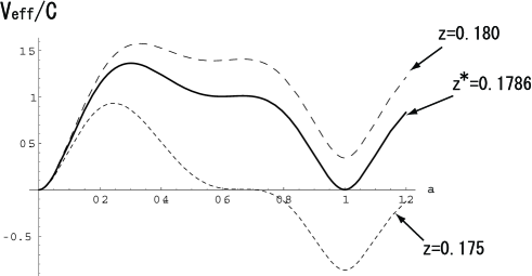
Figure 3: The behavior of the effective potential $V_{eff}(a)/C$ for a non-SUSY model with the matter content (25) is drawn with respect to $z\equiv RT$. The first phase transition of the two stage phase transitions is shown.

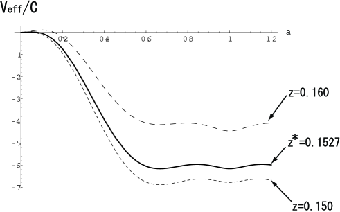
Figure 4: The behavior of the effective potential $V_{eff}(a)/C$ for a non-SUSY model with the matter content (25) is drawn with respect to $z\equiv RT$. The second phase transition of the two stage phase transition is shown.

The phase transition is the first order and the strength of the phase transition is obtained as

$${v(T_{1c})\over T_{1c}}=\left({{a_{0}^{T_{1c}}}\over{g_{4}R}}\right){1\over T_{1c}}={1\over g_{4}}{{a_{0}^{T_{1c}}}\over z_{1}^{*}}\simeq{1\over g_{4}}\times 5.599>1,$$ (29)

where

$$a_{0}^{T_{1c}}=1.0.$$ (30)

Let us note that, as before, the local minimum of the effective potential even at nonzero temperature is always located at $a_{0}^{T=T_{1c}}=1.0$.

As the temperature decreases further, the second phase transition occurs at

$$T_{2c}\simeq{1\over R}\times 0.1527\simeq g_{4}\times 56.088~{}~{}\mbox{GeV},$$ (31)

at which the vacua with the $U(1)^{\prime}\times U(1)$ gauge symmetry and the $U(1)_{em}$ gauge symmetry are degenerate (see figure 4). We obtain the strength of the phase transition in this case as

$${v(T_{2c})\over T_{2c}}={1\over g_{4}}{{\Delta a_{0}^{T}}\over z_{2}^{\star}}\simeq{1\over g_{4}}\times 2.183>1,$$ (32)

where $\Delta a_{0}^{T}\simeq 1.0-0.666667$. Let us also note that the local minima of the effective potential is again always located at $a_{0}^{T<T_{2c}}\simeq 0.6667$, which is the global minimum of the zero temperature part of the effective potential. This type of two stage phase transitions has never been observed in the scenario of the gauge-Higgs unification at finite temperature, and it is very interesting to consider physical applications of this type of the phase transition. We will see multi phase transition in the case of supersymmetric gauge models in the next section.

It has been known that fermions and/or the fermion belonging to the higher dimensional represenation, in general, tend to weaken the first order phase transition [17]. Here we confirm the statement is true from Eqs.(24), (29) and (32).

Before closing this section, we would like to mention the difference between the work by Panico and Serone [10] and ours. In their paper, a similar $SU(3)$ gauge model of gauge-Higgs unification at finite temperature was investigated and the first order electroweak phase transitions were obtained. In their model, in order to obtain the viable Higgs mass, two options were discussed, one is to introduce the bulk fields in the higher rank representation under $SU(3)$ gauge group (i.e. symmetric tensor), the other is to introduce localized gauge kinetic terms. However, the strength of the first order phase transition is at most $v(T_{c})/T_{c}\simeq 0.13(0.7)$ for the former(latter) option. On the other hand, as discussed in the text, there is no need to introduce bulk fields in the higher rank representation except for the adjoint one in our model. Furthermore, the strength of the phase transition is stronger (larger than the unity). Thus, we can conclude that our model is more favorable from the viewpoint of the application to the electroweak baryogenesis.

3 Supersymmetric gauge models

In this section, let us proceed to supersymmetric gauge models. We first study the phase transition for the the model considered in ref.[8]. As before, the degrees of freedom for the Wilson line phase is given by the parameter $a$ in Eq.(9). The effective potential for the phase at $T=0$ is given by

$$V_{eff}^{T=0}(a) = {{4\times\Gamma(5/2)}\over{{\pi^{5/2}(2\pi R)^{5}}}}\sum_{n=1}^{\infty}{1\over n^{5}}\left(1-\cos[2\pi n\beta]\right)$$ (33)

$$\times \Biggl{[}\left(-1+N_{adj}^{(+)}\right)\left(\cos[2\pi na]+2\cos[\pi na]\right)$$

$$+ N_{adj}^{(-)}\left(\cos[2\pi n(a-{1\over 2})]+2\cos[\pi n(a-1)]\right)$$

$$+ N_{fd}^{(+)}\cos[\pi na]+N_{fd}^{(-)}\cos[\pi n(a-1)]\Biggr{]},$$

where $\beta$ is the Scherk-Schwarz (SS) parameter which explicitly breaks supersymmmetry by the boundary condition for the $S^{1}$ direction for the gaugino and squarks in the supermultiplet [14]. As we can see, $\beta=0~{}(\mbox{mod}~{}1)$ yields the vanishing effective potential due to the recovery of the original supersymmetry.

Let us choose the flavor number and the SS parameter as

$$N_{adj}^{(+)}=2,~{}~{}N_{adj}^{(-)}=2,~{}~{}N_{fd}^{(+)}=0,~{}~{}N_{fd}^{(-)}=2,~{}~{}\beta=0.14.$$ (34)

In ref.[8], it has been shown that for the choice (34), the electroweak gauge symmetry is correctly broken, and the VEV is given by

$$a_{0}\simeq 0.0379.$$ (35)

The Higgs mass is obtained as

$$m_{H}^{2}\simeq\left(g_{4}^{2}\times 130~{}~{}\mbox{GeV}\right)^{2}.$$ (36)

We next consider the finite temperature effects. The effective potential at $T\neq 0$ is calculated as

$$V_{SUSY}^{T\neq 0}(a) = -\frac{2\times 4\Gamma(5/2)}{\pi^{5/2}(2\pi R)^{5}}\times\sum_{l=1}^{\infty}\sum_{n=1}^{\infty}\frac{1}{[(2\pi Rn)^{2}+l^{2}/T^{2}]^{5/2}}$$

$$\times \Biggl{[}\left(\tilde{J}^{(+)}[2a,\beta,n]+2\tilde{J}^{(+)}[a,\beta,n]\right)+N_{adj}^{(+)}\left(\hat{J}^{(+)}[2a,\beta,n]+2\hat{J}^{(+)}[a,\beta,n]\right)$$

$$+ N_{adj}^{(-)}\left(\hat{J}^{(-)}[2a,\beta,n]+2\hat{J}^{(-)}[a,\beta,n]\right)+N_{fd}^{(+)}\hat{J}^{(+)}[a,\beta,n]+N_{fd}^{(-)}\hat{J}^{(-)}[a,\beta,n]\Biggr{]},$$

where we have defined

$$\tilde{J}^{(+)}[a,\beta,n] \equiv (1-(-1)^{l}{\rm cos}(2\pi n\beta)){\rm cos}(\pi na),$$ (38)

$$\hat{J}^{(+)}[a,\beta,n] \equiv ({\rm cos}(2\pi n\beta)-(-1)^{l}){\rm cos}(\pi na),$$ (39)

$$\hat{J}^{(-)}[a,\beta,n] \equiv ({\rm cos}(2\pi n\beta)-(-1)^{l}){\rm cos}(\pi n(a-1)).$$ (40)

We observe that even if the SS parameter is zero we obtain the nonvanishing effective potential at the finite temperature due to the difference of statistics between bosons and fermions. The total effective potential we study is, then, given by

$$V_{SUSY}^{tot}(a)=V_{SUSY}^{T=0}(a)+V_{SUSY}^{T\neq 0}(a).$$ (41)

Let us note that $V_{SUSY}^{tot}(a)$ is invariant under $a\rightarrow-a$ and $a\rightarrow 2-a$, which means that it is enough to consider the region $0\leq a\leq 1$ .

In Figure 5, we show the behavior of $V_{SUSY}^{tot}(a)$ for various values of $z\equiv RT$.

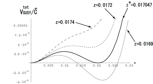
Figure 5: The behavior of the effective potential $V_{SUSY}^{tot}(a)/{\bar{C}}$ for a SUSY model with the matter content (34) is drawn with respect to $z\equiv RT$, where ${\bar{C}}\equiv 4\Gamma(5/2)/\pi^{5/2}(2\pi R)^{5}$.

Clearly, one can see that the phase transition is the first order, and the critical temperature, at which the two degenerate vacua appear, is given by

$$T_{c}\simeq{1\over R}\times 0.017047\simeq g_{4}\times 110.7~{}~{}\mbox{GeV},$$ (42)

where we have used (13). The relevant quantity to measure the strength of the phase transition is calculated as

$${v(T_{c})\over T_{c}}={1\over g_{4}}{{a_{0}^{T=T_{c}}}\over{z^{\star}}}\simeq{1\over g_{4}}\times 1.212>1,$$ (43)

where we have used the values $a_{0}^{T=T_{c}}=0.0206688$. The phase transition is so strong as to decouple the sphaleron process to leave the created baryon number after the electroweak phase transition.

Next let us choose the matter content with only fundamental representations as

$$N_{adj}^{(+)}=0,~{}~{}N_{adj}^{(-)}=0,~{}~{}N_{fd}^{(+)}=3,~{}~{}N_{fd}^{(-)}=0,~{}~{}\beta=0.14.$$ (44)

The minimum of the effective potential at zero temperature is given by the VEV

$$a_{0}=1.0,$$ (45)

for which the $SU(2)\times U(1)$ gauge symmetry is broken to $U(1)^{\prime}\times U(1)$. The mass of the scalar that respects the residual gauge symmetry is calculated as

$$m_{H}^{2}\simeq\left(g_{4}^{2}\times 18.03~{}~{}\mbox{GeV}\right)^{2}.$$ (46)

Figure 6: The behavior of the effective potential $V_{eff}^{tot}(a)/{\bar{C}}$ for a SUSY model with the matter content (44) is drawn with respect to $z\equiv RT$.

We see from Fig.5 that the phase transitions is the first order, and the critical temperature is calculated as

$$T_{c}\simeq{1\over R}\times 0.084\simeq g_{4}\times 20.66~{}~{}\mbox{GeV}.$$ (47)

Similar to the nonsupersymmetric case with the matter content (20), the local minimum of the effective potential before $T\geq T_{c}$ is always given by $a_{0}^{T\geq T_{c}}=1.0$. We next estimate the relevant quantity for the electroweak baryogenesis,

$${v(T_{c})\over T_{c}}={1\over g_{4}}{{a_{0}^{T=T_{c}}}\over{z^{\star}}}\simeq{1\over g_{4}}\times 11.90>1,$$ (48)

where we have used $a_{0}^{T=T_{c}}=1.0$ in Eq.(48). The phase transition is obviously found to be the first order.

Finally, let us consider the matter content with only adjoint representations,

$$N_{adj}^{(+)}=2,~{}~{}N_{adj}^{(-)}=0,~{}~{}N_{fd}^{(+)}=0,~{}~{}N_{fd}^{(-)}=0,~{}~{}\beta=0.14.$$ (49)

The minimum of the effective potential $V_{SUSY}^{T=0}$ is given by the VEV

$$a_{0}^{T=0}\simeq 0.6667,$$ (50)

and thus we have the correct pattern of electroweak symmetry breaking. The Higgs mass in this case is found to be very light as

$$m_{H}^{2}\simeq\left(g_{4}^{2}\times 17.91~{}~{}\mbox{GeV}\right)^{2}.$$ (51)

The phase structure at finite temperature is unexpectedly rich. There is a multi phase transition, in fact, we have four stages phase transitions for the matter content (49). It is too complicated to draw the behavior of the effective potential. Instead, let us show the behavior of the VEV, $a_{0}^{T\neq 0}$ in figure 7.

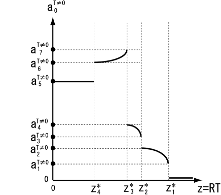
Figure 7: The behavior of the order parameter $a_{0}^{T\neq 0}$ for a SUSY model with the matter content (49) is drawn with respect to $z\equiv RT$.

Let us note that at the first phase transition, the vacua with the $SU(2)\times U(1)$ gauge symmetry and the $U(1)_{em}$ gauge symmetry is degenerate, but at the other three phase transitions, the vacua with the $U(1)_{em}$ are degenerate each other.

The critical temperature is obtained as

$$T_{ic}(i=1\sim 4)(\mbox{GeV})={1\over R}\times\left\{\begin{array}[]{l}z_{1}^{\star}=0.09832\\[8.5359pt] z_{2}^{\star}=0.09624\\[8.5359pt] z_{3}^{\star}=0.09616\\[8.5359pt] z_{4}^{\star}=0.08840\end{array}\right.=g_{4}\times\left\{\begin{array}[]{l}36.28006186\\[8.5359pt] 35.51254224\\[8.5359pt] 35.48302226\\[8.5359pt] 32.61958369,\end{array}\right.$$ (52)

where we have used (13). We also estimate the strength of each phase transition, which is given by

$${v(T_{ic})\over T_{ic}}={1\over g_{4}}{{\Delta a_{0}^{T=T_{c}}}\over{z_{i}^{\star}}}={1\over g_{4}}\times\left\{\begin{array}[]{ll}0.1336339/z_{1}^{\star}=1.35922498\\[8.5359pt] (0.262426-0.184866)/z_{2}^{\star}=0.80590191\\[8.5359pt] (0.865538-0.271745)/z_{3}^{\star}=6.17505199\\[8.5359pt] (0.79899-0.666667)/z_{4}^{\star}=1.49686652,\end{array}\right.$$ (53)

where $\Delta a_{0}^{T=T_{c}}\equiv{\left|{a_{0}^{T=T_{jc}}-a_{0}^{T=T_{kc}}}\right|}$ stands for the jump between the two VEV’s at the critical temperature $z_{i}^{\star}(i=1\sim 4)$. We see that except for the second phase transition, the phase transitions are the strong first order. It is interesting to consider the application of the multi phase transition.

4 Conclusions

We have studied the phase transition in gauge-Higgs unification at finite temperature in a certain class of gauge models, including supersymmetric ones. Since the dynamics of the gauge-Higgs unification is essentially the Coleman-Weinberg mechanism, the phase transition is strongly expected to be the first order. We have, in fact, observed that the phase transition is the first order, and the strength becomes stronger as the Higgs mass becomes lighter in models under consideration.

We have also found an interesting phase transition patterns, which has never been reported in the theory of the gauge-Higgs unification for an $SU(3)$ gauge theory with only adjoint fermions. There have been two stage phase transitions characterized by the two critical temperatures $T_{1c}$ and $T_{2c}$. At each critical temperature, it is turned out that the phase transition is the first order. The vacua with the $SU(2)\times U(1)$ gauge symmetry and the $U(1)^{\prime}\times U(1)$ gauge symmetry are degenerate at $T=T_{c1}$, while at $T=T_{2c}(<T_{1c})$, the vacua with the $U(1)^{\prime}\times U(1)$ symmetry and the $U(1)_{em}$ gauge symmetry are degenerate. It is interesting to consider if there are applications of these two stage phase transitions.

We have also studied supersymmetric gauge models with the Scherk-Schwarz supersymmetry breaking. We have found that the phase transition is strongly the first order for the simple matter content (34) which provides with the correct pattern of electroweak symmetry breaking and the Higgs mass of the correct order of magnitude. We have also studied the phase transition for the matter content with supermultiplets only in the fundamental representation (44) and only in the adjoint representation (49). We have found the same phase transition pattern as the case for non-SUSY gauge model with the corresponding matter content (20) for the matter content (44). On the other hand, for the matter content (49), we have obtained the multi phase (four in the case) transitions.

Contrary to the non-SUSY models, we have a free parameter in SUSY models, the SS parameter $\beta$ in addition to the number of flavors. In ref.[8] it has been pointed out that the magnitude of $\beta$ affects the size of the Higgs mass, so that it is very interesting to study how the strength of the phase transition depends on the SS parameter. This will be reported in a separated paper. Finally, in order to understand the phase structure of the theory of gauge-Higgs unification more deeply, it is necessary to study the effect of chemical potential $\mu$ [19]. If we introduce the chemical potential for a fermion, for example, the effective potential for the fermion is modified as

$$V_{F}^{\mu} = (-1)^{F}(r2^{[D/2]}){1\over 2}(-1)\sum_{n=1}^{\infty}\Biggl{[}{{2\Gamma(D/2)}\over{(2\pi Rn)^{D}\pi^{D/2}}}\cos[2\pi n(Qa-{1\over 2}\delta)]$$

$$- \frac{2\pi^{D\over 2}}{\Gamma(D/2)(2\pi R)^{D}}\left(n+Qa-\frac{\delta}{2}\right)^{D-1}\int_{1}^{\infty}dy~{}(y^{2}-1)^{{D\over 2}-1}\left({1\over{1+{\rm e}^{{\bar{z}}y+{\mu\over T}}}}+(\mu\leftrightarrow-\mu)\right)\Biggr{]},$$

where ${\bar{z}}\equiv 2\pi(n+Qa-\delta/2)/2\pi RT,~{}Q={1\over 2}~{}(1)$ for matter belonging to the fundamental (adjoint) representations under the $SU(3)$ gauge group and $\delta$ takes $+1$ or $-1$, depending on the intrinsic parity. Since this potential is very complicated, we are particularly interested in the behavior of the effective potential in the limit of $T\rightarrow 0$. This work is in progress, and we hope that interesting results will be soon reported elsewhere.

Acknowledgements

N.M. is supported by Special Postdoctral Researchers Program at RIKEN (No. A12-61014). K.T. would thank the professors, K. Funakubo and Y. Hosotani for valuable discussions. K.T. is supported by the $21$st Century COE Program at Osaka University.

References

- [1] N. S. Manton, Nucl. Phys. B158 141 (1979), D. B. Fairlie, Phys. Lett. 82B (1979) 97.
- [2] N. V. Krasinikov, Phys. Lett. 273B (1991) 731, H. Hatanaka, T. Inami and C.S. Lim, Mod. Phys. Lett. A13 (1998) 2601, N. Arkani-Hamed, A. G. Cohen and H. Georgi, Phys. Lett. 513B (2001) 232, G. R. Dvali, S. Randjbar-Daemi and R. Tabbash, Phys. Rev. D65 (2002) 064021, I. Antiniadis, K. Benakli and M. Quiros, New J. Phys. 3, (2001),20.
- [3] Y. Hosotani, Phys. Lett. 126B (1983) 309, Ann. Phys. (N.Y.) 190, 233 (1989).
- [4] K. Takenaga, Phys. Rev. D64 (2001) 066001, Phys. Rev. D66 (2002) 085009, L. J. Hall, Y. Nomura and D. R. Smith, Nucl. Phys. B639 (2002) 307, G. Burdman and Y. Nomura, Nucl. Phys. B656 (2002) 3, M. Kubo, C. S. Lim and H. Yamashita, Mod. Phys. Lett. A17 (2002) 2249. N. Haba and Y. Shimizu, Phys. Rev. D67 (2003) 095001, C. Csaki, C. Grojean, H. Murayama, Phys. Rev. D67 (2003) 085012 I. Gogoladze, Y. Mimura, S. Nandi and K. Tobe, Phys. Lett. 575B (2003) 66, L. Pilo and J. Terning, Phys. Rev. D69 (2004) 055006, K. Choi, N. Haba, K. S. Jeong, K. Okumura, Y. Shimizu and M. Yamaguchi, J. High Energy Phys.0402, 037 (2004), Y. Hosotani, S. Noda and K. Takenaga, Phys. Rev. D69 (2004) 125014, Phys. Lett. 607B (2005) 276, N. Haba, K. Takenaga and T. Yamashita, Phys. Lett. 605B (2005) 355, Phys. Rev. D71 (2005) 025006, K. Oda and A. Weiler, Phys. Lett. 606B (2005) 408, Y. Hosotani and M. Mabe, hep-ph/0503020.
- [5] K. Hasegawa, C. S. Lim and N. Maru, Phys. Lett. 604B (2004) 133.
- [6] S. Coleman and E. Weinberg, Phys. Rev. D7 (1973) 1888.
- [7] N. Haba, Y. Hosotani, Y. Kawamura and T. Yamashita, Phys. Rev. D70 (2004) 015010.
- [8] N. Haba, K. Takenaga and T. Yamashita, hep-ph/0411250, To appear in Phys. Lett. B.
- [9] K. Funakubo, A. Kakuto and K. Takenaga, Prog. Theor. Phys. 91 (1994) 341, and references therein.
- [10] G. Panico and M. Serone, hep-ph/0502255.
- [11] C. A. Scucca, M. Serone and L. Silvestrini, Nucl. Phys. B669 (2003) 128,
- [12] For a review see, A. Cohen, D. Kaplan and A. Nelson, Ann. Rev. Nucl. Part. Sci. 43 (1993)27, K. Funakubo, Prog. Theor. Phys. 96 (1996) 475, V. A. Rubakov and M.E. Shaposhnikov, Phys. Usp. 39 (1996) 461, (hep-ph/9603208).
- [13] K. Funkaubo and S. Tao, hep-ph/0501052.
- [14] J. Scherk and J.H. Schwarz, Phys. Lett. 82B (1979) 60, P. Fayet, Phys. Lett. 159B (1985) 121, Nucl. Phys. B263 87 (1986), K. Takenaga, Phys. Lett. 425B (1998) 114, Phys. Rev. D58 (1998) 026004.
- [15] H. Hata and T. Kugo, Phys. Rev. D21 (1980) 3333.
- [16] N. Haba, M. Harada, Y. Hosotani and Y. Kawamura, Nucl. Phys. B657 (20169) 03, Erratum, ibid. B669 (2003) 381.
- [17] L. Dolan and R. Jackiw, Phys. Rev. D9 (1974) 3320.
- [18] C-L. Ho and Y. Hosotani, Nucl. Phys. B345 445 (1990).
- [19] A. Actor, Phys. Lett. 157B (1985) 53, C-C. Lee and C-L. Ho, Mod. Phys. Lett. A8 (1993) 1495, K. Shiraishi, Zeit. Phys. C35, 37 (1987).