Testing a new mesh refinement code in the evolution of a spherically symmetric Klein-Gordon field

Abstract.

Numerical evolution of the spherically symmetric, massive Klein-Gordon field is presented using a new adaptive mesh refinement (AMR) code with fourth order discretization in space and time, along with compactification in space. The system is non-interacting thus the initial disturbance is entirely radiated away. The main aim is to simulate its propagation until it vanishes near ${\mycal I}^{+}$. By numerical investigations of the violation of the energy balance relations, the space-time boundaries of “well-behaving” regions are determined for different values of the AMR parameters. An important result is that mesh refinement maintains precision in the central region for longer time even if the mesh is only refined outside of this region. The speed of the algorithm was also tested, in case of 10 refinement levels the algorithm was two orders of magnitude faster than the extrapolated time of the corresponding unigrid run.

1. Introduction

The primary motivation to develop the presented techniques and perform the associated investigations is the need for the efficient simulation of nonlinear dynamical systems. Numerical integration of nonlinear field equations is a difficult problem even if the metric is fixed. An obvious complication is that the field propagates in infinite space-time, but the computational resources are finite. Fortunately, infinity can be brought to finite distance by compactifying space-time, with a conformal rescaling of the metric [1]. A well-chosen coordinate transformation can also increase the efficiency of numerical calculations. However, a good transformation is often hard to find, especially when time evolution changes the system drastically, or in the presence of more than two different scales. Some examples are black hole formation, black hole merger, compact binary stars, etc. The sizes of such gravitational radiation sources are very small compared to the produced wavelength, which is much smaller than the distance from the detector. Different length scales must be considered simultaneously, but it is extremely hard if time evolution is simulated on a uniform grid. Adaptive mesh refinement (AMR) algorithms overcome these difficulties by using a coarse base grid which is refined automatically at “interesting” locations for more precise calculation [2].

The precision also depends on the order of numerical schemes used. According to Hübner, fourth order calculations are at least two orders of magnitude more efficient than second order [3]. Nevertheless, only second order calculations are known to be used by AMR codes in numerical relativity so far, although several implementations of the algorithm were developed since Choptuik’s pioneering work [4]. Our choice of the fourth order Runge-Kutta scheme is also supported by the result of Hansen, Khokhlov and Novikov. They found that among the methods they investigated, this is the most efficient one in terms of accuracy and dissipation [5].

Problems where gravity is coupled to matters fields are complicated to start with, thus the code will be applied first to study simpler systems, physical fields in flat space-time. The simplest possible massive field is the free Klein-Gordon field, the time evolution of which is investigated in case of spherical symmetry in this paper. This system is known to provide certain surprises in numerical simulations [6], moreover there is a straightforward means of checking the efficiency of the developed numerical method by making use of the analytic solution to the initial value problem.

However, in contrast to the usual scenarios, there is no compact central object in this system that could keep any part of the initial disturbance from radiating away. Instead of studying the central region where vibration with decreasing amplitude is left behind, the aim is the simulation of the field at larger distances, where a hypothetical detector could be placed. As the wave propagates outwards and approaches ${\mycal I}^{+}$, its wavelength approaches zero, partly due to a physical effect [6], partly because of the space compactification. Hence for an accurate simulation of the long-range behavior, finer and finer subgrids are needed as the wave gets closer to ${\mycal I}^{+}$.

Interaction will be included in forthcoming studies. Plans include the verification of earlier numerical results on the logarithmic decay of $\phi^{4}$ breathers [7] and the study of excitations of Bogomol’nyi-Prasad-Sommerfield magnetic monopoles. In the latter case, a previous study [8] will be extended by the inclusion of the Higgs field’s self interaction. In both of these settings, nonlinear massive fields evolve in fixed Minkowski space-time.

2. The AMR algorithm

The code is based on the Berger-Oliger algorithm [2]. At the initial time ($T=0$), it starts with a uniform grid, where the values in the grid points are determined by the initial condition. Based on local error estimations of the first integration step, child grids may be generated and filled with values of the initial condition function. This procedure is applied recursively, until either the local error becomes lower than the chosen tolerance in each point or the maximum refinement level is reached. In later integration steps, if a refinement level contains point(s) with relatively large errors, then finer levels are regridded in child to parent order (finest first). When a level is regridded, new points are interpolated using old points from the same level and the parent level.

The same refinement ratio $r$ is used on each level. For the refinement criteria, Richardson error estimation of an arbitrarily chosen function $u$ is used. The grid is refined if

(1) $$\frac{|u(Q_{\Delta t,\Delta x}^{2}f(x,t))-u(Q_{2\Delta t,2\Delta x}f(x,t))|}{2^{q+1}-2}>\varepsilon\Delta t,$$

where $Q_{\Delta t,\Delta x}$ is the numerical integration operator, $f(x,t+\Delta t)\simeq Q_{\Delta t,\Delta x}f(x,t)$, $q$ is the order of the method, $f$ is the field and $\varepsilon$ is the error tolerance (see [2]). The exact form of $u$ proved to be irrelevant, provided that it has an approximate linear dependence on the field components. For example, the square root of the energy density was a good choice in Klein-Gordon simulations, but the value of field $f$ was equally good. For simplicity, I choose the latter in all simulations.

To reach high precision in the numerical calculations, only symmetric finite difference and interpolation schemes are used whenever it is possible. Space interpolation is simplified by aligning new subgrids with their parent grid. Time interpolation can be avoided in one space dimension, because it is possible to apply relatively large grid margins without noticeable efficiency loss. The initial subgrid margin is proportional to $r$ and it shrinks in each step, until the time becomes equal to the time on the enclosing coarser grid. (See Fig. 1.) Then the new values on the margin are determined by space interpolation.

Because of the above-mentioned proportionality, $r$ should not be too large, otherwise the large margin sizes could result in unnecessary slowdown. In case of a larger refinement ratio, less refined levels are needed for the same precision, but a smaller $r$ has the benefit that the mesh can adapt more closely to the solution. In my tests, simulations using double refinement were slightly more efficient (by about 5%) than triple refinement, thus I choose $r=2$.

Figure 1. Subgrid margin narrowing in case of $r=2$ and 4th order Runge-Kutta. Margin points -28, …, -1 at $t$, $t+2\Delta t$, $t+4\Delta t$ etc. are calculated by interpolation of points in the coarse (parent) grid.

For time and space discretization, the same order of accuracy was used. Second order Runge-Kutta time integration with second order space discretization and third order space interpolation, fourth order Runge-Kutta with fourth order space discretization and fifth order interpolation. The presented numerical results are calculated in fourth order. A fourth order centered finite difference scheme uses 5=2+1+2 points, thus the numerical error propagates 2 points in each step. However, to avoid instabilities, an artificial dissipation term containing the sixth order sixth derivative was also applied  [3]:

(2) $$\sigma f^{\prime\prime\prime\prime\prime\prime}(\Delta x)^{5}\ =\ \sigma\cdot(f_{k-3}-6f_{k-2}+15f_{k-1}-20f_{k}+15f_{k+1}-6f_{k+2}+f_{k+3})/\Delta x,$$

where I used $\sigma=0.01$. It increases error propagation velocity to 3 points per step.

Therefore refined grid margins must be shrunk by 3 points in each step. The fourth order Runge-Kutta method consists of 4 substeps, thus the overall loss of refined margin points is $12r=24$ in a coarse time step, see Fig. 1. However, a 24-point wide margin would not be sufficient if the refined and the coarse grid have their origins (zero index points) or right edges at the same location. After a coarse time step, the coarse margin shrinks to 24-12=12 points. Although the leftmost refined margin point (with index $i_{\mathrm{refined}}=-24$) coincides with the leftmost coarse margin point ($i_{\mathrm{coarse}}=-12$) at this time, its neighbor ($i_{\mathrm{refined}}=-23$) is not in a lucky position, it must be interpolated from coarse margin points. Fifth order centered interpolation requires 3 points on both sides, but there is only one coarse point ($i_{\mathrm{coarse}}=-12$) on the left side in this case. Choosing a slightly wider initial margin, with at least 28 points, can solve this problem. Then the coarse margin shrinks to 28-12=16 points which is enough to interpolate all refined margin points.

For the fifth order interpolation of field values at point $k$, the following formula is used:

(3) $$f_{k}\,\ =\,\ \frac{A_{0}f_{i_{0}}+A_{1}f_{i_{1}}+A_{2}f_{i_{2}}+A_{3}f_{i_{3}}+A_{4}f_{i_{4}}+A_{5}f_{i_{5}}}{\sum_{i}A_{i}},$$

where $i_{0}$, …, $i_{5}$ are the indexes of the six known points (from the coarse grid and the previous refined grid) and $A_{0}$, …, $A_{5}$ are coefficients. The 6 coefficients are determined by fixing the function values, the derivatives and the second derivatives in points $i_{2}$ and $i_{3}$. (Derivatives are approximated in fourth order of accuracy from 2+1+2 points.) Their values depend on the distance (and existence) of the nearest old fine grid.

Table 1. Fifth order interpolation coefficients.

0	1	2	3	4	5	6	7	8	9	10	$A_{0}$	$A_{1}$	$A_{2}$	$A_{3}$	$A_{4}$	$A_{5}$	$\sum_{i}A_{i}$
$i_{0}$		$i_{1}$		$i_{2}$	$k$	$i_{3}$		$i_{4}$		$i_{5}$	3	-25	150	150	-25	3	256
$i_{0}$		$i_{1}$		$i_{2}$	$k$	$i_{3}$	$i_{4}$	$i_{5}$	$\cdot$	$\cdot$	15	-116	690	1020	-384	55	1280
$i_{0}$	$i_{1}$	$i_{2}$	$k$	$i_{3}$		$i_{4}$		$i_{5}$			55	-384	1020	690	-116	15	1280

The possible cases are shown in Table 1.

3. Simulation of a Klein-Gordon field

A free, spherically symmetric Klein-Gordon field is described by the equation

(4) $$\partial_{t}^{2}\Phi-\frac{1}{r}\partial_{r}^{2}(r\Phi)+m^{2}\Phi\,\ =\,\ 0,$$

where $m$ is the mass parameter and Minkowski metric is used, $ds^{2}=dt^{2}-dr^{2}-r^{2}d\sigma^{2}$.

Fodor and Rácz [6] have shown that for arbitrary initial data with compact support the evolution of this system can be characterized by the formation of self similarly expanding shells built up of high frequency oscillations:

(5) $$\Phi(t,r)\,\ \approx\,\ t^{-3/2}\Psi_{\dot{\Phi}_{0}}(r/t)\cos\left(m\sqrt{t^{2}-r^{2}}+\frac{\pi}{4}\right),$$

where $\pm\Psi_{\dot{\Phi}_{0}}(r/t)$ are the contours of the shells; the form of this function depends on the initial condition. An important property of this solution is that both the frequency and the wave number of oscillations on the outer shell grows proportionally to $\sqrt{t}$. To prove it, we determine these quantities as the partial derivatives of the cosine’s argument:

(6) $$\omega\,\ = \,\ \frac{\partial(m\sqrt{t^{2}-r^{2}})}{\partial t}\,\ =\,\ \frac{mt}{\sqrt{t^{2}-r^{2}}},$$

(7) $$k\,\ = \,\ -\frac{\partial(m\sqrt{t^{2}-r^{2}})}{\partial r}\,\ =\,\ \frac{mr}{\sqrt{t^{2}-r^{2}}}.$$

The outer edge expands with the velocity of light, $r\approx t$, hence the frequency in a short distance $\Delta r=t-r$ from the outer edge is approximately equal to the wave number, their values can be estimated using the following formula:

(8) $$\omega\,\ \approx\,\ k\,\ \approx\,\ \frac{mt}{\sqrt{(\Delta r)(t+r)}}\,\ \approx\,\ \frac{m\sqrt{t}}{\sqrt{2\Delta r}}.$$

To remove the $1/r$ coordinate singularity from Eq. 4, the “unphysical” field

(9) $$f(t,r)\ =\ r\Phi(t,r)$$

is used instead of $\Phi$. Space is compactified using a transformation as in Refs.[8, 9]:

(10) $$T(t,r)\ =\ \omega t-\sqrt{\omega^{2}r^{2}+1},\quad R(r)\ =\ \frac{\sqrt{\omega^{2}r^{2}+1}-1}{\omega r},$$

where $-\infty<T<\infty$ and $0\leq R<1$.

To simplify numerical calculations, the second derivatives are removed from the field equation by introducing the partial derivatives of $f$ as new variables $f_{T}$ and $f_{R}$. Then the field equation (4) can be written as a system of 3 first order partial differential equations and a constraint condition:

(11) $$\partial_{T}f\ = \ f_{T},$$

$$\partial_{T}f_{T}\ = \ -\frac{1-R^{2}}{1+R^{2}}f_{T}-\frac{R(3+R^{2})(1-R^{2})}{2(1+R^{2})}f_{R}-2R\partial_{R}f_{T}+\frac{(1-R^{2})^{2}}{4}\partial_{R}f_{R}$$

(12) $$-\begin{cases}\frac{1}{\omega^{2}}\left(\frac{1+R^{2}}{1-R^{2}}\right)^{2}m^{2}f,&\text{if }R\neq 1,\\ 0,&\text{if }R=1,\end{cases}$$

(13) $$\partial_{T}f_{R}\ = \ \partial_{R}f_{T},$$

(14) $$f_{R}\ = \ \partial_{R}f.$$

Boundary conditions. For the numerical calculation of derivatives near $R=0$, information on the parity properties of the functions must be applied. Whenever the field $\Phi$ is smooth, it has to be an even function of $R$. Hence $f$ and $f_{T}$ are odd and $f_{R}$ is even:

(15) $$f(-R)\ =\ -f(R),\quad f_{T}(-R)\ =\ -f_{T}(R),\quad f_{R}(-R)\ =\ f_{R}(R).$$

The behavior of function $f$ near the other boundary is also important for similar reasons. The field $\Phi$ vanishes in ${\mycal I}^{+}$, thus the function values for $R\geq 1$ points are supposed to vanish too:

(16) $$f(R)\ =\ 0,\quad f_{T}(R)\ =\ 0,\quad f_{R}(R)\ =\ 0.$$

The initial condition is a smooth, motionless hunch on the $T(t,r)=0$ hypersurface:

(17) $$f\ = \ \begin{cases}c\cdot\exp\left(\frac{d}{(r-a)^{2}-b^{2}}\right)&\text{if }r>a-b\text{ and }r<a+b\\ 0&\text{otherwise},\end{cases}$$

(18) $$f_{T}\ = \ 0.$$

In the simulations, I used a hunch at $R\simeq 0.050\pm 0.037$, with parameters $\omega=0.05$, $a=2$ (center of hunch in $r$), $b=1.5$ (half-width in $r$), $c=70$ and $d=10$.

Figure 2. Penrose diagram of a part of the Minkowski space-time, with the $R$, $T$ coordinate lines. Initial condition is specified on the $T=0$ spacelike hypersurface (thick line). A null geodesic from the origin $(R,T)=(0,0)$ reaches ${\mycal I}^{+}$ at $T=1$ (dashed line). A numerical solution preserves initial energy with 99% precision under its “validity limit” (upper thick lines).

This disturbance is initially close to the origin, thus it is expected to reach ${\mycal I}^{+}$, the future null infinity, at about $T\simeq 1$ like the null geodesic denoted by dashed line on Fig. 2.

4. Results

Figure 3. Exact (thin dashed lines) and numerically calculated field values (bold lines) on the $T=5$ hypersurface. The top plot shows the result of a unigrid simulation with 256 grid points. The right edge is calculated more precisely, with 6 levels of refinement (middle). An even closer look with 10 levels of refinement is shown on the bottom plot.

The simulations reproduced the most important feature of the analytical result by Fodor and Rácz [6], the self similarly expanding shells built up of higher frequency oscillations. The amplitudes of these high frequency “carrier waves” are modulated by the $\Psi_{\dot{\Phi}_{0}}$ function in Eq. (5). As the shells expand and approach ${\mycal I}^{+}$, the $R$-length (the wavelength in $R$ coordinate units) of the carrier wave approaches zero, thus finer and finer grids are needed to simulate its propagation. Accordingly, to zoom into the vicinity of $R=1$, the number of refinement levels must be increased, see Fig. 3.

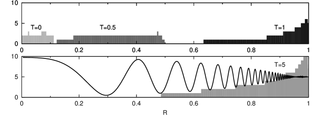
Figure 4. Number of mesh refinement levels as a function of $R$ in different time slices. The top plot shows the refinement in $T=0,\ 0.5,\ 1$ (gray boxes), the bottom plot shows both the refinement in $T=5$ (gray boxes) and the form of the $\Phi$ function (black curve).

At $T=0$, the grid is only refined in a small range enclosing the initial hunch. Then the refinement follows the $\Phi$ waves, it moves outwards and expands. When the waves approach ${\mycal I}^{+}$, the peak of the refinement level function begins to increase, see Fig. 4. Since the exact solution of the current problem is known, it might be possible to replace mesh refinement by a uniform mesh together with a clever time dependent coordinate transformation. The mesh refinement structure shown on Fig. 4 foreshadows the complications in finding such a transformation in space; a hunch like this cannot be smoothed using a simple, monotonous function for $T<1$. There are complications also for $T>1$, because the frequency of oscillations on the outer shell increases in time (see Eq. (8)). Moreover, even if an easily calculable transformation exists which makes mesh refinement unnecessary, the equal time surfaces would be different with the new coordinates, making it hard to transform the results back to the $(T,R)$ system.

Convergence. The 4th order convergence of the algorithm was verified by calculating the

Figure 5. Time dependence of the absolute error and the convergence factor in AMR and unigrid simulations.

time dependence of the convergence factor

(19) $$Q\ =\ \frac{||f_{\Delta R}-f||}{||f_{\Delta R/2}-f||},$$

where $||\cdot||$ is the $L^{2}$ norm and $f_{\Delta R}$ is the numerical solution of function $f$ in case of a base grid with $\Delta R$ spacing. Locations and sizes of refined subgrids are stored and reused in calculations with the finer base grids ($\Delta R/2$). Fig. 5 shows the absolute errors and the convergence factor for some unigrid and AMR simulations. The $\log_{2}Q$ curves start with a plateau at a height of approximately $4$, proving fourth order convergence. However, the order of convergence falls off near $T\simeq 1$ because of the abrupt increase of absolute error when the wave reaches future null infinity (${\mycal I}^{+}$) and the $R$-length of oscillations reaches zero, making even the finest mesh resolution insufficient.

Figure 6. Energy conservation bounds of numerical solutions calculated using different number of refinement levels and different error tolerance settings.

Energy conservation is violated numerically as the $R$-length of waves approaching ${\mycal I}^{+}$ decrease below grid resolution. To check this, the following quantity is calculated instead of total energy:

(20) $$E(T_{\mathrm{max}},R_{\mathrm{max}})=\intop_{0}^{R_{\mathrm{max}}}dR\,\varepsilon(T_{\mathrm{max}},R)+\intop_{0}^{T_{\mathrm{max}}}dT\,j_{E}(T,R_{\mathrm{max}}),$$

where $\varepsilon$ is the energy density and $j_{E}$ is the energy flow. Numerically lost energy is mostly contained in the second term. By substituting $R_{\mathrm{max}}=1$, we get the total energy which is not conserved numerically. To “restore energy conservation” at a given $T$, $R_{\mathrm{max}}$ must be decreased. Both $T_{\mathrm{max}}$ and $R_{\mathrm{max}}$ have a critical value below which energy is conserved with acceptable precision: $E/E_{0}\simeq 1$, where $E_{0}=E(0,1)$. Above the critical values, energy is lost: $E/E_{0}<1$. Fig. 6 shows the energy contour lines on the $T_{\mathrm{max}}-R_{\mathrm{max}}$ plane where only 95% or 99% of the initial energy is conserved: $E/E_{0}=0.95,0.99$. The conservation bound can be pushed outwards both in $R_{\mathrm{max}}$ and $T_{\mathrm{max}}$ by increasing the number of refinement levels.

Figure 7. Time dependence of the error in the $R\leq R_{\mathrm{max}}=0.375$ “central” range.

Central range. As time evolves, the wave packet propagates outwards, leaving less and less matter in the center. The amplitude of oscillations decrease asymptotically as $t^{-3/2}\propto T^{-3/2}$ (see Refs. [6, 10]). Function $f$ and its derivatives also decrease, thus one may suppose that a unigrid simulation is enough here. I tested this assumption by performing unigrid (256, 512 and 4096 points) and AMR simulations (256 points on base grid, 1 and 4 refinement levels). Errors and the norm of function $f$ were calculated by restricting integrations to $R\leq R_{\mathrm{max}}=0.375$. Most of the matter leaves this range before $T\approx 1$, thus function $f$ becomes “smoother” and the grid is not refined at later times here. Consequently, the error of the $\Delta R=1/256$ unigrid and the same base resolution AMR simulations are close for a while. However, the unigrid error starts to increase much faster at about $T\approx 12$. This abrupt degradation proves that error can propagate inwards from outside ($R>R_{\mathrm{max}}$). Hence the unigrid error is only “acceptable” for $T<20$, while the 4-level AMR calculation reaches the same level of inaccuracy much later, at about $T\approx 150$. See the curves with labels “$256$” and “$256\times 2^{4}$” on Fig. 7. On the same plot, it can also be seen that the error of a high precision unigrid run is smaller than that of the corresponding AMR with the same maximum precision. Compare the curve labeled with “512” (unigrid) to the “$256\times 2^{1}$” curve (AMR, 1.5 times faster), and “$4096$” to “$256\times 2^{4}$” (AMR, 4 times faster). However, the AMR error curve increases much slower than the unigrid error curve, hence they meet at a certain time after which AMR is more accurate. If the AMR error tolerance is small enough, then the error at their meeting point is also small.

Note that by restricting attention to the central range in $R$, a much longer simulation was possible in $T$. This feature can also be seen on the energy conservation curves on Fig. 6, where $T_{\mathrm{max}}$ increases when $R_{\mathrm{max}}$ is decreased.

Table 2. Speed comparison of unigrid and AMR runs from $T=0$ to $5$. The “$n$” columns contain the number of points on the (spacelike) base grid. Run times ($t_{0}$ and $t_{\mathrm{AMR}}$) were measured on AMD Opteron (64 bit) 1.8 GHz hardware and Sun Java 1.5.0_02 virtual machine. $N_{0}$ and $N_{\mathrm{AMR}}$ are the total number of points of the spacetime grid. ^∗Instead of performing unigrid runs with 32768 and more grid points, their times were extrapolated using the time of the $n=16384$ run and assuming $t_{\mathrm{unigrid}}\propto n^{2}$.

unigrid		AMR
			error tolerance
			$10^{-8}$	$2\cdot 10^{-8}$	$10^{-7}$
$n$	$t_{0}$	$n\times r^{levels}$	$t_{\mathrm{AMR^{\prime}}}$	$t_{\mathrm{AMR}}$	$t_{\mathrm{AMR^{\prime\prime}}}$	$N_{0}/N_{\mathrm{AMR}}$	$t_{0}/t_{\mathrm{AMR}}$
256	5.9s
512	22.5s	$256\times 2^{1}$	18.8s	17.6s	17.3s	1.7	1.3
1024	73s	$256\times 2^{2}$	56s	46s	38s	2.7	1.6
2048	295s	$256\times 2^{3}$	118s	108s	84s	4.5	2.7
4096	1407s	$256\times 2^{4}$	293s	263s	194s	7.7	5.3
8192	5597s	$256\times 2^{5}$	630s	586s	468s	12.9	9.6
16384	22360s	$256\times 2^{6}$	1577s	1416s	1164s	20.9	15.8
32768	89440s∗	$256\times 2^{7}$	4110s	3574s	2916s	32	25
65536	357760s∗	$256\times 2^{8}$	10904s	9590s	8202s	48	37
131072	1431040s∗	$256\times 2^{9}$	29064s	26614s	21427s	72	54
262144	5724160s∗	$256\times 2^{10}$	70148s	63562s	47825s	116	90

Speed tests. The time of a unigrid simulation is proportional to the total number of grid points in the spacetime domain:

(21) $$t_{\mathrm{run}}\propto 1/(\Delta x)^{d},$$

where $\Delta x\propto 1/n$ is the grid spacing and $d$ is the number of dimensions of the spacetime grid, $d=2$ in this case. When using AMR, the same resolution can be reached much faster because only a small part of the grid is refined. In case of 10 refinement levels, AMR would be two orders of magnitude faster than a corresponding unigrid run. AMR/unigrid run time ratios can be approximated by calculating the ratio of the total number of grid points in the spacetime domain ($N_{0}$ for unigrid and $N_{\mathrm{AMR}}$ for AMR), then adding the overhead ($\sim 30\%$) of the AMR algorithm. The $t_{\mathrm{AMR}}/t_{0}\sim 1.3N_{\mathrm{AMR}}/N_{0}$ formula is a good approximation for the measured times in Table 2, in case of 5 or more refinement levels. The formula (21) can be fitted nicely to AMR run times also. These fittings were performed at constant error tolerance values ($10^{-8}$, $2\cdot 10^{-8}$ and $10^{-7}$) for simplicity. The result is that for small $T_{\mathrm{max}}$ values, the “effective dimension” $d$ increases with $T_{\mathrm{max}}$ until a plateau is reached near $T_{\mathrm{max}}=5$, at a height of $d=1.35\pm 0.04$.

5. Other tests

Further testing was performed with nonlinear 1 dimensional Klein-Gordon fields and periodic boundary conditions, $\Phi(x\pm 1)=\Phi(x)$, by adding a fourth order self interaction term to the Lagrangian:

(22) $$L\,\ =\,\ {1\over 2}(\partial_{t}\Phi)^{2}-{1\over 2}(\partial_{x}\Phi)^{2}-\frac{m^{2}}{2}\Phi^{2}-{c_{4}\over 4}\Phi^{4}.$$

The initial condition at $t=0$ is the motionless hunch used earlier in Eqs. (17-18) but substituting $r$ by $x$, $f$ by $\Phi$, $f_{T}$ by $\Phi_{t}$ and using the parameter values $a=0.5$, $b=0.2$, $c=10$, $d=1$. Test problems include massive ($m^{2}=1$, $c_{4}=\frac{1}{3}$ and $m^{2}=10$, $c_{4}=\frac{10}{3}$), massless ($m^{2}=0$), free ($c_{4}=0$) cases and the sine-Gordon field:

(23) $$L\,\ =\,\ {1\over 2}(\partial_{t}\Phi)^{2}-{1\over 2}(\partial_{x}\Phi)^{2}+m^{2}(\cos\Phi-1).$$

In each of these cases, the initial hunch at $x=0.5$ splits and its two parts propagate in opposite directions. At $t=0.5$ they reach the periodic boundaries $x=0,\,1$ where they pass through each other. They meet again at $(t,x)=(1,\ 0.5)$, almost restoring the initial state but in a distorted form. As a consequence of the translation invariance and the lack of nonlinear coordinate transformations, the derivatives and the numerical error do not increase substantially during the movement of the hunches, the number of required mesh refinement levels for a given error tolerance is determined by the initial state and preserved later.

Another test was performed with the $\phi^{4}$ breather described by the Lagrangian:

(24) $$L(\phi,\partial_{t}\phi,\partial_{x}\phi)\,\ =\,\ \frac{1}{2}(\partial_{t}\phi)^{2}-\frac{1}{2}(\partial_{x}\phi)^{2}-\frac{1}{4}(\phi^{2}-1)^{2}.$$

For the numerical simulation of this system, I compactified space using the same transformation as earlier in Eq. (10), $R=R(x)$ with $\omega=0.05$. Time $t$ is not transformed. The initial condition is the same as that used by Geicke [7], it contains a kink and an antikink in $x=\pm 0.8$. The radiation of the initial “kick” involves the outwards propagation of a wave with decreasing $R$-length. As it propagates outwards, more and more levels of refinement are activated until it vanishes (in $t\gtrsim 10^{3}$ if the base grid spacing is $\Delta R\leq 1/128$). Then only the smooth, stable, oscillating wave remains near the origin and refinement is no longer needed. I performed simulations without further energy loss until $t=10^{7}$ using a $\Delta R=1/128$ base grid. However, I found energy loss in case of finer base grids. I also found that increased precision in the simulation of the initial radiation does not necessarily increase precision near the origin in the long run. The same amount of energy disappears with the same rate if mesh refinement is not used at all in case of $\Delta R=1/384$ and $t\leq 7000$. Further experimenting is needed for the verification of the statement of Geicke [7] about the logarithmic decay of this system.

6. Summary

A new AMR code was developed for integrating field equations numerically in time. It is tested thoroughly using fourth order Runge-Kutta method and fourth order space discretization, but it is also possible to use other numerical schemes. The main test problem is the simulation of a spherically symmetric Klein-Gordon field in a special coordinate system (10) with compactified space coordinate. The exact solution of this problem is known, thus it is possible to calculate the absolute error of the numerical simulation. By calculating the errors of AMR simulations with different base grid spacings, the fourth order convergence of the algorithm was shown. The numerical violation of energy conservation was also investigated; I determined the space-time boundaries of the “well-behaving” range. Inside this space-time volume, the sum of the total energy and its integrated outgoing flux is constant with an acceptable precision. The time boundary $T_{\mathrm{max}}$ is a monotonically decreasing function of the maximum space coordinate $R_{\mathrm{max}}$ (see Fig. 6). It means that energy is conserved numerically for longer time if a smaller central range is examined in space. The error of the simulation behaves similarly; longer runs can be “closer” to the exact solution if the error norm is calculated only in a small central range. The speed of the algorithm was also tested, in case of 10 refinement levels the AMR algorithm was two orders of magnitude faster than the extrapolated time of the corresponding unigrid run.

References

- [1] J. Frauendiener, Living Rev. Relativity 7 (2004) 1. http://www.livingreviews.org/lrr-2004-1/
- [2] M. J. Berger and J. Oliger, J. Comput. Phys. 53 (1984) 484-512.
- [3] P. Hubner, Class. Quant. Grav. 16 (1999) 2823-2843.
- [4] M. W. Choptuik, Phys. Rev. Lett. 70 (1993) 9-12.
- [5] J. Hansen, A. Khokhlov, I. Novikov, Int. J. Mod. Phys. D13 (2004) 961.
- [6] G. Fodor and I. Rácz, Phys. Rev. D68 (2003) 044022.
- [7] J. Geicke, Phys. Rev. E49 (1994) 3539-3542.
- [8] G. Fodor and I. Rácz, Phys. Rev. Lett. 92 (2004) 151801.
- [9] V. Moncrief, Proc. of the Workshop on Mathematical Issues in Numerical Relativity, Santa Barbara (2000), http://online.itp.ucsb.edu/online/numrel00/moncrief/
- [10] S. Hod and T. Piran, Phys. Rev. D58 (1998) 044018.