Taming the Tachyon
in Cubic String Field Theory

Abstract:

We give evidence based on level-truncation computations that the rolling tachyon in cubic open string field theory (CSFT) has a well-defined but wildly oscillatory time-dependent solution which goes as $e^{t}$ for $t\rightarrow-\infty$. We show that a field redefinition taking the CSFT effective tachyon action to the analogous boundary string field theory (BSFT) action takes the oscillatory CSFT solution to the pure exponential solution $e^{t}$ of the BSFT action.

1 Introduction

The tachyon of the open bosonic string has played an important role in recent years in the development of string field theory as a background-independent formulation of string theory. Following Sen’s conjectures regarding this tachyon [1], significant progress has been made towards demonstrating that both the unstable vacuum containing the tachyon and the “true” vacuum where the tachyon has condensed are well-defined states in Witten’s cubic open string field theory (CSFT) [2]. This is important evidence that string field theory is capable of describing multiple distinct vacuum configurations using a single set of degrees of freedom, as one would expect for a background-independent formulation of the theory. Some of the work in this area is reviewed in [3, 4].

An important aspect of the open string tachyon which is not yet fully understood, however, is the dynamical process through which the tachyon rolls from the unstable vacuum to the stable vacuum. A review of previous work on this problem is given in [4]. Computations using CFT, boundary states, RG flow analysis and boundary string field theory (BSFT) [5, 6, 7, 8] show that the tachyon should monotonically roll towards the true vacuum, but should not arrive at the true vacuum in finite time [9]-[16]. In BSFT variables, where the tachyon $T$ goes to $T\rightarrow\infty$ in the stable vacuum, the time-dependence of the tachyon field goes as $T(t)=e^{t}$. This dynamics is intuitively fairly transparent, and follows from the fact that $e^{t}$ is a marginal boundary operator [17, 18, 19, 9, 16]. Other approaches to understanding the rolling tachyon from a variety of viewpoints including DBI-type actions [20]-[23], S-branes and timelike Liouville theory [24]-[28], matrix models [29]-[34], and fermionic boundary CFT [35] lead to a similar picture of the time dynamics of the tachyon.

In CSFT, on the other hand, the rolling tachyon dynamics appears much more complicated. In [36], Moeller and Zwiebach used level truncation to analyze the time dependence of the tachyon. They found that at low levels of truncation, the tachyon rolls well past the minimum of the potential, then turns around and begins to oscillate with ever increasing amplitude. It was further argued by Fujita and Hata in [37] that such oscillations are a natural consequence of the form of the CSFT equations of motion, which include an exponential of time derivatives acting on the tachyon field.

These two apparently completely different pictures of the tachyon dynamics raise an obvious puzzle. Which picture is correct? Does the tachyon converge monotonically to the true vacuum, or does it undergo wild oscillations? Is there a problem with the BSFT approach? Does the CSFT analysis break down for some reason such as a branch point singularity at a finite value of $t$? Does the dynamics in CSFT behave better when higher-level states are included? Is CSFT an incomplete formulation of the theory?

In this paper we resolve this puzzle. We carry out a systematic level-truncation analysis of the tachyon dynamics for a particular solution in CSFT. We compute the trajectory $\phi(t)$ as a power series in $e^{t}$ at various levels of truncation. We show that indeed the dynamics in CSFT has wild oscillations. We find, however, that the trajectory $\phi(t)$ is well-defined in the sense that increasing both the level of truncation in CSFT and the number of terms retained in the power series in $e^{t}$ leads to a convergent value of $\phi(t)$ for any fixed $t$, at least below an upper bound $t<t_{b}$ associated with the limit of our computational ability.

We reconcile this apparent discrepancy with the results of BSFT by demonstrating that a field redefinition which takes the CSFT action to the BSFT action also maps the wildly oscillating CSFT solution to the well-behaved BSFT exponential solution. This qualitative change in behavior through the field redefinition is possible because the field redefinition relating the tachyon in the two formulations is nonlocal and includes terms with arbitrarily many time derivatives. Such field redefinitions are generically expected to be necessary when relating the background-independent CSFT degrees of freedom to variables appropriate for a particular background [38]. A similar field redefinition involving higher derivatives was shown in [39] to be necessary to relate the massless vector field $\hat{A}_{\mu}$ of CSFT on a D-brane with the usual gauge field $A_{\mu}$ appearing in the Yang-Mills and Born-Infeld actions. Other approaches to the rolling tachyon using CSFT appear in [40]-[43]; related approaches which have been studied include $p$-adic SFT [44, 45], open-closed SFT [46], and vacuum string field theory [47, 48]. Closed string production during the rolling process is described in [49, 50, 51].

The paper is organized as follows. Section 2 describes the general approach that we use to find the rolling tachyon solution and gives the leading order terms in the solution explicitly. Section 3 describes the results of numerically solving the equations of motion in level-truncated CSFT. Section 4 is dedicated to finding the leading terms in the field redefinition that relates the effective tachyon actions in Boundary and Cubic String Field Theory. Section 5 contains conclusions and a discussion of our results. Some technical details regarding our methods of calculation are relegated to Appendices.

As this paper was being completed the paper [52] appeared, which treats the same system, although without considering massive fields. The analysis of [52] is carried out using analytic methods which give an approximate rolling tachyon solution when all fields other than the tachyon are neglected. The solution in their paper shares some qualitative features with our results—in particular, they find a solution which has similar behavior for negative time, and their solution also rolls past the naive minimum of the tachyon potential. Their solution has a cusp at $t=0$ where the solution has a discontinuous first derivative; we believe that their solution breaks down at this point, but that their solution is good for $t<0$ and that the analytic methods they use in deriving their results are of interest and may help in understanding the dynamics of the system.

2 Solving the CSFT equations of motion

We are interested in finding a solution to the complete open string field theory equations of motion. The full CSFT action contains an infinite number of fields, coupled through cubic terms which contain exponentials of derivatives (see [3] for a detailed review). Thus, we have a nonlocal action in which it is difficult to make sense of an initial value problem (see [53, 54, 55, 56] for some discussion of such equations with infinite time derivatives).

Nonetheless, we can systematically develop a solution valid for all times by assuming that as $t\rightarrow-\infty$ the solution approaches the perturbative vacuum at $\phi=0$. In this limit the equation of motion is the free equation for the tachyon field $\ddot{\phi}(t)=\phi(t)$, with solution $\phi(t)=ce^{t}$. For $t\ll 0$, we can perform a perturbative expansion in the small parameter $e^{t}$. The computations carried out in this paper indicate that this power series indeed seems convergent for all $t$. A related approach was taken in [36, 37], where an expansion in $\cosh t$ was proposed. This allows a one-parameter family of solutions with $\dot{\phi}(0)=0$, but is more technically involved due to the more complicated structure of $\cosh nt$ compared with $e^{nt}$. We restrict attention here to the simplest case of solutions which can be expanded in $e^{t}$, but we expect that a more general class of solutions can be constructed using this approach. Note that in most previous work on this problem, solutions have been constructed using Wick rotation of periodic solutions; in this paper we work directly with the real solution which is a sum of exponentials.

The infinite number of fields of CSFT represents an additional complication. We can, however, systematically integrate out any finite set of fields to arrive at an effective action for the tachyon field which we can then solve using the method just described. We do this using the level-truncation approximation to CSFT including fields up to a fixed level. We find that the resulting trajectory $\phi(t)$ converges well for fixed $t$ as the level of truncation is increased.

We thus compute the solution $\phi(t)$ with the desired behavior $e^{t}$ as $t\rightarrow-\infty$ in two steps. In the first step, described in subsection 2.1, we compute the tachyon effective action, eliminating all the other modes using equations of motion. Some technical details of this calculation are relegated to Appendix A. In the second step, described in subsection 2.2, we write down the equation of motion for the effective theory and solve it perturbatively in powers of $e^{t}$.

2.1 Computing the effective action

We are interested in a spatially homogeneous rolling tachyon solution. One can compute such a solution by solving the equations of motion for the infinite family of string fields with all the spatial derivatives set to $0$. Labeling string fields $\psi_{i}$, the cubic string field theory equations of motion (in the Feynman-Siegel gauge) take the schematic form

$$(\partial_{t}^{2}-m_{i}^{2})\psi_{i}(t)=g\,e^{V^{11}_{00}(\partial^{2}_{s}+\partial^{2}_{u}+\partial_{s}\partial_{u})}C_{i}^{jk}(\partial_{u},\partial_{s})\ \psi_{j}(s)\psi_{k}(u)|_{s=u=t}$$ (1)

where all possible pairs of fields appear on the RHS. The coefficients $C_{ijk}$ multiplying each term may contain a finite order polynomial in the derivatives $\partial_{s},\partial_{u}$. Plugging in the Ansatz $\phi(t)=\psi_{0}(t)=e^{t}+\cdots$ with all other fields vanishing at order $e^{t}$ it is clear that we can systematically solve the equations for all fields order by order in $e^{t}$. This is one way of systematically solving order by order for $\phi(t)$.

We will find it convenient to think of the perturbative solution for $\phi(t)$ in terms of an effective action $S[\phi]$ which arises by integrating out all the massive string fields at tree level. Perturbatively, we can solve the equations of motion (1) for all fields except $\phi=\psi_{0}$ as power series in $\phi$, by recursively plugging in the equations of motion for all fields except $\phi$ on the RHS until all that remains is a perturbative expansion in terms of $\phi(t)$ and its derivatives. We have used two approaches to compute the effective action $S[\phi]$. One approach is to explicitly use the equations (1) for all fields up to a fixed level. This approach is useful for generating terms to high powers in $g$ but becomes unwieldy for fields at high levels. The second approach we use is to compute the effective action as a diagrammatic sum using the level truncation on oscillator method developed in [57]. This approach is useful for calculating low-order terms in the effective potential where high-level fields are included. Some details of the oscillator approach are described in Appendix A.

The leading terms in the tachyon action are the quadratic and cubic terms coming directly from the CSFT action

$$S[\phi]=\frac{1}{2}\int dt\;\phi(t)\left(-\partial_{t}^{2}+1\right)\phi(t)-\frac{g}{3}\left(e^{\frac{1}{2}V^{11}_{00}(\partial_{t}^{2}-1)}\phi(t)\right)^{3}+\cdots$$ (2)

where

$$V^{11}_{00}=-\log\left(\frac{27}{16}\right)$$ (3)

is the Neumann coefficient for the three tachyon vertex.

Integrating out the massive fields at tree level gives rise to higher-order terms $g^{2}\phi^{4},\ldots$ with even more complicated derivative structures. The resulting effective action can be written in terms of the (temporal) Fourier modes $\phi(w)$ of $\phi(t)$ as

$$S[\phi]=\sum_{n}\frac{g^{n-2}}{n!}\int\prod_{i=1}^{n}dw_{i}\;(2\pi)^{n}\delta\Bigl{(}\sum_{i}w_{i}\Bigr{)}\Xi_{n}^{\text{CSFT}}(w_{1},\dots,w_{n})\phi(w_{1})\dots\phi(w_{n})$$ (4)

where the functions $\Xi_{n}^{CSFT}(w_{1},\dots,w_{n})$ determine the derivative structure of the terms at order $g^{n-2}\phi^{n}$. The quadratic and cubic terms following from (2) are

$$\Xi^{\text{CSFT}}_{2}(w_{1},w_{2}) =(1-w_{1}w_{2}),$$ (5)

$$\Xi^{\text{CSFT}}_{3}(w_{1},w_{2},w_{3}) =-2\,e^{-\frac{1}{2}V^{11}_{00}(w_{1}^{2}+w_{2}^{2}+w_{3}^{2}+3)}.$$ (6)

One way to obtain the approximate classical effective action for the tachyon field is to use the equations of motion for a few low level massive fields to eliminate these fields explicitly from the action. The higher level massive fields are set to zero (level truncation).

As an example, we now explicitly compute the quartic term in the effective action (4) in the level 2 truncation. In the case of CSFT for a single D-brane the combined level of fields coupled by a cubic interaction must be even. For example, there is no vertex coupling two tachyons (level zero) with the gauge boson (level 1). It follows that there are no tree level Feynman diagrams with all external tachyons and internal fields of odd level. Thus, in calculating the tachyonic effective action we may set odd level fields to 0. Fixing Feynman-Siegel gauge, the only fields involved are the tachyon $\phi$ and three level 2 massive fields with $m^{2}=1$: $\beta$, $B_{\mu}$ and $B_{\mu\nu}$. The terms in the action contributing to the four-tachyon term in the effective action are

$$\frac{1}{2}\int dt\,\beta(\partial_{t}^{2}+1)\beta-B_{\mu\nu}(\partial_{t}^{2}+1)B^{\mu\nu}-B_{\mu}(\partial_{t}^{2}+1)B^{\mu}+\\ g\int dt\,a_{1}\tilde{\phi}^{2}\tilde{B}_{\mu}^{\mu}+a_{2}(\tilde{\phi}\partial_{t}\partial_{t}\tilde{\phi}-\partial_{t}\tilde{\phi}\partial_{t}\tilde{\phi})\tilde{B}^{00}+a_{3}\tilde{\phi}^{2}\tilde{\beta}+a_{4}\tilde{\phi}\partial_{t}\tilde{\phi}\tilde{B}^{0}$$ (7)

where $\tilde{f}=e^{\frac{1}{2}V_{00}^{11}(\partial^{2}_{t}-1)}f$. Other interaction terms involving level 2 fields, for example $\beta^{3}$ or $B_{\mu}B^{\mu}\phi$, would contribute to the effective action at higher powers of $\phi$. The coefficients $a_{1}$, … $a_{4}$ are real numbers and can be expressed via the appropriate matter and ghost Neumann coefficients,

$$a_{1} =-\frac{V_{11}^{11}}{\sqrt{2}}\approx 0.130946, a_{2} =\sqrt{2}(V_{01}^{12})^{2}\approx 0.419026,$$

$$a_{3} =X_{11}^{11}\approx 0.407407, a_{4} =-6V_{02}^{12}\approx 0.628539.$$ (8)

Following the procedure described above we write down the equations of motion for the massive fields, and plug them into (7). We then obtain a quartic term in the tachyonic effective action,

$$g^{2}e^{-3V_{00}^{11}}\int\prod_{i=1}^{4}{(2\pi dw_{i})}\phi(w_{i})\delta(\sum w_{i})\frac{\exp\big{(}-V_{00}^{11}[w_{1}^{2}+w_{2}^{2}+w_{3}^{2}+w_{4}^{2}+w_{1}w_{2}+w_{3}w_{4}]\big{)}}{1-(w_{1}+w_{2})^{2}}\\ \Bigl{(}b_{1}+b_{2}\,w_{2}(w_{2}-w_{1})+b_{3}\,w_{1}w_{4}(w_{2}-w_{1})(w_{4}-w_{3})+b_{4}\,w_{2}w_{4}\Bigr{)},$$ (9)

where we have denoted

$$b_{1} =\frac{1}{2}(13(V_{11}^{11})^{2}-(X_{11}^{11})^{2}), b_{2} =-V_{11}^{11}(V_{01}^{12})^{2},$$

$$b_{3} =(V_{01}^{12})^{4}, b_{4} =18(V_{02}^{12})^{2}.$$ (10)

We have explicitly computed the terms to order $\phi^{7}$ in the effective tachyon action in the $L=2$ truncation. One can in principle continue the procedure further, increasing both the level of truncation and the powers of $\phi$ in the effective action. Explicit calculation, however, becomes laborious as we take into account more and more string field components; the oscillator method [57], described in the appendix A is more efficient for high-level computations. In the next section we proceed to find the solution of the equations of motion from the effective tachyon action.

2.2 Solving the equations of motion in the effective theory

We now outline the process for solving the tachyon equation of motion for the effective theory, and we compute the first perturbative corrections to the free solution. The variation of the effective action (4) gives equations of the form

$$(\partial_{t}^{2}-1)\phi=\sum_{n=2}^{\infty}g^{n-1}K_{n}(\phi,\dots,\phi)$$ (11)

where the nonlinear terms of order $\phi^{n}$ are denoted by $K_{n}$. The specific form of the $K_{n}$ follow by differentiating (4) with respect to $\phi(t)$. The functions $\Xi_{n}$ appearing in (4), and thus the corresponding $K_{n-1}$’s can in principle be explicitly computed for arbitrary $n$ at any finite level of truncation using the method described in the previous subsection. An alternate approach which is more efficient for computing $K_{n}$ at small $n$ but large truncation level is reviewed in Appendix A. In general, independently of the method used to compute it, $K_{n}$ will be a complicated momentum-dependent function of its arguments.

The solution of the linearized equations of motion which satisfies the boundary condition $\phi\rightarrow 0$ as $t\rightarrow-\infty$ is $\phi(t)=c_{1}e^{t}$. As discussed above, we wish to use perturbation theory to find a rolling solution which is defined by this asymptotic condition as $t\rightarrow-\infty$. Note that this asymptotic form places a condition on all derivatives of $\phi$ in the limit $t\rightarrow-\infty$, as appropriate for a solution of an equation with an unbounded number of time derivatives. If we now assume that the full solution can be computed by solving (11) using perturbation theory, at least in some region $t<t_{\text{max}}$, it can be easily seen that the successive corrections to the asymptotic solution $\phi_{1}(t)=c_{1}e^{t}$ are of the form $\phi_{n}(t)=c_{n}e^{nt}$. In other words, to solve the equations of motion using perturbation theory we expand $\phi(g,t)$ in powers of $g$

$$\phi(g,t)=\phi_{1}(t)+g\phi_{2}(t)+g^{2}\phi_{3}(t)+\dots$$ (12)

where

$$\phi_{n}(t)=c_{n}e^{nt}.$$ (13)

As we will see, our assumption leads to a power series which seems to be convergent for all $t$ and all $g$. Note that since $g^{n}e^{nt}=e^{n(t+\log(g))}$, the coupling constant can be set to 1 by translating the time variable and rescaling $\phi$, so convergence for fixed $g$ and all $t$ implies convergence for all $t$ and for all $g$. Plugging (12) into (11) we find

$$(\partial_{t}^{2}-1)\phi_{n}=(n^{2}-1)c_{n}e^{nt}=\sum_{p}\sum_{m_{1}+m_{2}+\dots m_{p}=n}K_{p}(\phi_{m_{1}},\phi_{m_{2}},\dots,\phi_{m_{p}}).$$ (14)

These equations allow us to solve for $c_{n>1}$ iteratively in $n$. Having solved the equations for $c_{2},\ldots,c_{n-1}$ we can plug them in via (13) on the right hand side of (14) to determine $c_{n}$.

As an example, let us consider the first correction $\phi_{2}(t)=c_{2}e^{2t}$ to the linearized solution $\phi_{1}(t)=c_{1}e^{t}$. The equation of motion at quadratic order arising from $K_{2}$ is

$$(\partial_{t}^{2}-1)\phi=-e^{\frac{1}{2}V^{11}_{00}(\partial_{t}^{2}-1)}(e^{\frac{1}{2}V^{11}_{00}(\partial_{t}^{2}-1)}\phi)^{2}.$$ (15)

Plugging in $\phi_{1}=c_{1}e^{t}$, $\phi_{2}=c_{2}e^{2t}$ we find

$$c_{2}(\partial_{t}^{2}-1)e^{2t}=-c_{1}^{2}e^{\frac{1}{2}V^{11}_{00}(\partial_{t}^{2}-1)}(e^{\frac{1}{2}V^{11}_{00}(\partial_{t}^{2}-1)}e^{t})^{2}$$ (16)

and therefore

$$c_{2}=-\frac{1}{3}e^{\frac{3}{2}V^{11}_{00}}c_{1}^{2}.$$ (17)

If we normalize $c_{1}=1$ then the solution to order $e^{2t}$ is

$$\phi(t)=e^{t}-\frac{64}{243\,{\sqrt{3}}}e^{2\,t}+\dots\ .$$ (18)

The quartic interaction term in the effective action would contribute to coefficients $c_{n}e^{nt}$ with $n\geq 3$ with the leading order contribution being $c_{3}e^{3t}$. From equation (14) we have

$$c_{3}=\frac{e^{-3t}}{8}\left(2c_{2}K_{2}(e^{t},e^{2t})+K_{3}(e^{t},e^{t},e^{t})\right).$$ (19)

where $K_{3}$ is obtained by differentiating (9) with respect to $\phi(t)$. The two summands in (19) represent contributions from the cubic and quartic terms in the effective action. The numerical values of these contributions are

$$(\delta c_{3})_{\text{cubic}} \cong 0.0021385, (\delta c_{3})_{\text{quartic}} \cong 0.0000492826.$$ (20)

It is perhaps surprising that the contribution to $c_{3}$ from the quartic term in the effective action is merely $0.2\%$ of the contribution from the cubic term. Adding the contributions we get the rolling solution to second order in perturbation theory in level 2 truncation

$$\phi(t)\cong e^{t}-0.152059e^{2\,t}+0.002187\,e^{3\,t}+\dots\ .$$ (21)

In this section we have explicitly demonstrated our procedure for the calculation of the rolling tachyon solution. We considered the CSFT action truncated to fields with level less or equal than two and computed the first two corrections to the solution of the linearized equations of motion. The next section is dedicated to the more detailed numerical analysis of the rolling tachyon solution.

3 Numerical results

In this section we describe the results of using the level-truncated effective action $S[\phi]$ to compute approximate perturbative solutions to the equation of motion through (14). We are testing the convergence of the solution in two respects. In subsection 3.1 we check that the solution converges nicely at fixed $t$ when we take into account successively higher powers of $\phi$ in a perturbative expansion of the effective action while keeping the truncation level fixed at $L=2$. In subsection 3.2 we check that the solution converges well for fixed $t$ when we keep the order of perturbation theory fixed while increasing the truncation level.

3.1 Convergence of perturbation theory at $L=2$

The equation (14) allows us to find the successive perturbative contributions to the solution of the equations of motion, given an explicit expression for the terms in the effective action. The solution takes the form

$$\phi(t)=\sum_{n}c_{n}e^{nt}.$$ (22)

Since all the derivatives of $e^{nt}$ are straightforward to compute, as in (17), we can replace these derivatives in any operator through $f(\partial_{t})e^{nt}\rightarrow f(n)e^{nt}$. This manipulation is justified as long as $f$ is regular at $n$.

We have computed the functions $\Xi_{n}^{{\rm CSFT}}$ and the resulting $K_{n-1}$’s by solving the equations of motion up to $n=7$ and integrating out all fields at truncation level $L=2$ as described in subsection 2.1. We have used these $K_{n}$’s to compute the resulting approximate coefficients $c_{n}$, with $n\leq 6$. To compute the coefficient $c_{n}$ one needs the effective tachyon action computed to order $n+1$; higher terms in the action contribute only to higher order coefficients.

Figure 1: The solution $\phi(t)$ including the first two turnaround points, including fields up to level $L=2$. The solid line graphs the approximation $\phi(t)=e^{t}+c_{2}e^{2t}$. The long dashed line graphs $\phi(t)=e^{t}+c_{2}e^{2t}+c_{3}e^{3t}$. The approximate solutions computed up to $e^{4t}$, $e^{5t}$ and $e^{6t}$ are very close in this range of $t$ and are all represented in the short dashed line. One can see that after going through the first turnaround point with coordinates $(t,\phi(t))\sim$ (1.27, 1.8) the solution decreases, reaching the second turnaround at around $(t,\phi(t))\sim$ (3.9, -81). The function $f(\phi(t))=\text{sign}(\phi(t))\log(1+|\phi(t)|)$ is graphed to show both turnaround points clearly on the same scale.

The $L=2$ approximation to the solution for the tachyon field is

$$\phi(t)\cong e^{t}-\frac{64\,e^{2\,t}}{243\,{\sqrt{3}}}+0.002187\,e^{3\,t}-\\ 3.9258\,{10}^{-6}\,e^{4\,t}+4.9407\,{10}^{-10}\,e^{5\,t}+6.3227\,{10}^{-12}\,e^{6\,t}.$$ (23)

Plotting the result we observe that for small enough $t$ the term $e^{t}$ dominates and the solution decays as $e^{t}$ at $-\infty$. Then, as $t$ grows, the second term in (23) becomes important. The solution turns around and $\phi(t)$ becomes negative, with the major contribution coming from $e^{2t}$. Then the next mode, $e^{3t}$ becomes dominating and so on. The solution $\phi(t)$ around the first two turnaround points is shown on the figure 1. Note that the trajectory passes through the minimum of the static potential, which is at $\phi\sim 0.545$ [58, 59], well before the first turnaround point.

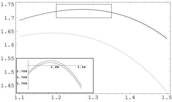
Figure 2: First turnaround point for the solution in $L=2$ truncation scheme. The large plot shows the approximations with $\phi^{3}$ (the gray line), $\phi^{4}$ (black solid), and $\phi^{5}$ (dashed lines) terms in the action taken into account. The smaller plot zooms in on the approximations with $\phi^{4}$ and $\phi^{5}$ terms taken into account. The corrections from higher powers of $\phi$ are very small and the corresponding plots are indistinguishable from the one of the $\phi^{5}$ approximation.

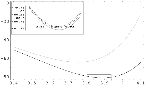
Figure 3: Second turnaround point for the solution in $L=2$ truncation scheme. The gray line on the large plot shows the solution computed with the effective action including terms up to $\phi^{4}$. The black solid and dashed lines represent higher order corrections. On the small plot the solid line includes $\phi^{5}$ corrections, the dotted line includes corrections from the $\phi^{6}$ term and the dashed line takes into account the $\phi^{7}$ term.

The positions of the first $2$ turnaround points are quite accurately determined by taking into account the effective action terms up to $\phi^{5}$. The inclusion of the higher order terms in the action changes the position of the first $2$ turnaround points only slightly. Figures 2 and 3 illustrate the dependence of the position of the first two turnaround points on the powers of $\phi$ included in effective action. We interpret these results as strong evidence that, at least for the effective action at truncation level $L=2$, the solution (22) is given by a perturbative series in $e^{t}$ which converges at least as far as the second turnaround point, and plausibly for all $t$.

3.2 Convergence of level truncation

From the results of the previous subsection, we have confidence that the first two points where the tachyon trajectory turns around are well determined by the $\phi^{4}$ and $\phi^{5}$ terms in the effective action. To check whether these oscillations are truly part of a well-defined trajectory in the full CSFT, we must check to make sure that the turnaround points are stable as our level of truncation is increased and the terms in the effective action are computed more precisely. From previous experience with level truncated calculations of the static effective tachyon potential and the vector field effective action [59, 57, 39], where coefficients in the effective action generically converge well, with errors of order $1/L$ at truncation level $L$, we expect that the full tachyon effective action will also converge well and will lead to convergent values of $c_{n}$ within a factor of order 1 of the $L=2$ results computed explicitly.

We have computed the $\phi^{4}$ term in the effective action at levels of truncation up to $L=16$. The results of this computation for the approximate trajectory $\phi(t)$ are shown in Figure 4, which demonstrates the behavior of the first turnaround point as we include higher level fields. This computation shows that the first turnaround point is already determined to within less than $1\%$ by the level $L=2$ truncation. This turnaround point is also in close agreement with the computations of [36]. We take this computation as giving strong evidence that this turnaround point is real. We expect from analogy with other level truncation computations of effective actions and potentials that the other terms in the effective action considered here will also generally converge well. Combining the explicit result for the $\phi^{4}$ term at high levels of truncation with the computation of the previous subsection, we have (to us) convincing evidence that the perturbative expansion $e^{nt}$ for the rolling tachyon solution is valid well past the first turnaround point, and that the level truncation procedure converges to a trajectory containing this turnaround point. Extrapolating the results of this computation, we believe that the qualitative phenomenon of wild oscillations revealed by the level $L=2$ computation is a correct feature of the time-dependent tachyon trajectory in CSFT, and that more precise calculations at higher level will only shift the positions of the turnaround points mildly, leaving the qualitative behavior intact.

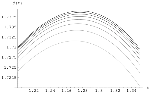
Figure 4: The figure shows the convergence of the solution around the first turnaround point as we increase the truncation level. Bottom to top the graphs represent the approximate solutions computed with the effective action computed up to $\phi^{4}$ and truncation level increasing in steps of 2 from $L=2$ to $L=16$. We observe that the turnaround point is determined to a very high precision already at the level 2. Similar behavior is observed for the second turnaround point.

It is interesting to compare the behavior of the perturbative expansion of this time-dependent tachyon solution with a perturbative expansion of the effective tachyon potential $V(\phi)$. As found in [59], the power series expansion for $V(\phi)$ fails to converge beyond $|\phi|\sim 0.1$ due to a branch point singularity at negative $\phi$ where the Feynman-Siegel gauge choice breaks down [60]. Although the potential can be continued for positive $\phi$ past the radius of convergence using the method of Padé approximants [61], another branch point associated with the breakdown of Feynman-Siegel gauge is encountered at a positive $\phi$ just past the minimum near $\phi\sim 0.545$. Because of these branch points, the expansion for the effective potential is badly behaved past these points; unlike the time-dependent solution we have studied here, there is no sense in which the potential $V(\phi)$ converges for a general fixed value of $\phi$. While we initially thought that the wild oscillations of the low-level computation of the tachyon trajectory $\phi(t)$ might indicate a similar breakdown of the perturbative expansion, our results at higher levels seem to give conclusive evidence that this is not the case. This suggests that the Feynman-Siegel gauge choice is valid in the region of field space containing the trajectory $\phi(t)$ for all $t$ even though the corresponding static $\phi$ lies outside the region of gauge validity.

4 Taming the tachyon with a field redefinition

Now that we have confirmed that CSFT gives a well-defined but highly oscillatory time-dependent solution, we want to understand the physics of this solution. Although the oscillations seem quite unnatural from the point of view of familiar theories with only quadratic kinetic terms and a potential, the story is much more subtle in CSFT due to the higher-derivative terms in the action. For example, while the tachyon field apparently rolls into a region with $V(\phi)\gg V(0)=0$, the energy of the perturbative rolling tachyon solution we have found is conserved, as we have verified by a perturbative calculation of the energy including arbitrary derivative terms, along the lines of similar calculations in [36].

To understand the apparently odd behavior of the rolling tachyon in CSFT, it is useful to consider a related story. In [39] we computed the effective action for the massless vector field on a D-brane in CSFT by integrating out the massive fields. The resulting action did not take the expected form of a Born-Infeld action, but included various extra terms with higher derivatives which appeared because the degrees of freedom natural to CSFT are not the natural degrees of freedom expected for the CFT on a D-brane, but are related to those degrees of freedom by a complicated field redefinition with arbitrary derivative terms. In principle, we expect such a field redefinition to be necessary any time one wishes to compare string field theory computations (or any other background-independent formulation) with CFT computations in any particular background. The necessity for considering such field redefinitions was previously discussed in [38, 62].

Thus, to compare the complicated time-dependent trajectory we have found for CSFT with the marginal $e^{t}$ perturbation of the boundary CFT found in [9, 10], we must relate the degrees of freedom of BSFT and CSFT through a field redefinition which can include arbitrary derivative terms. Given an explicit form $S[T]$ for the BSFT effective tachyon action which admits a solution $T(t)=e^{t}$, we can construct a perturbative field redefinition $\phi(t)=\Phi(T(t))$ which maps the BSFT effective action $S[T]$ to the CSFT effective tachyon action $S[\phi]$. Since such a field redefinition must map a solution of the field equations in one picture to a solution in the other picture, it follows that this map takes the BSFT solution $T(t)=e^{t}$ to the perturbative solution $\phi(t)$ of the CSFT effective action. In this section we use an explicit formulation of the BSFT effective action to compute the leading terms of the field redefinition relating the effective field theories for $T(\phi)$, the tachyon field in boundary string field theory and $\phi$, the tachyon in cubic string field theory. This computation shows in a concrete example how the complicated dynamics we have found for the tachyon in CSFT maps to the simple dynamics of BSFT associated with the marginal deformation $e^{t}$.

In our explicit computations, we use the effective tachyonic action of BSFT computed up to cubic order in [63]; another approach to computing the BSFT action which may apply more generally was developed in [64]. As we have just discussed, we expect that a similar field redefinition can be constructed for any BSFT effective tachyon action. The BSFT action is determined via the partition function for the boundary SFT and the tachyon’s beta function. Thus the particular form of the action depends on the renormalization scheme for the boundary CFT. The BSFT tachyon $T$ we use here is, therefore, the renormalized tachyon with the renormalization scheme of [63]. We now proceed to construct a perturbative field redefinition relating the CSFT and BSFT effective actions. We then will check explicitly that the field redefinition maps the rolling tachyon solution $T(t)=e^{t}$ to the leading terms in the perturbative solution $\phi(t)=e^{t}-\frac{64}{243\,{\sqrt{3}}}e^{2\,t}+\cdots$ which we have computed in the previous section. The fact that the field redefinition is nonsingular at $T=e^{t}$ is consistent with the Ansatz $\sum_{n}c_{n}e^{nt}$ for the rolling tachyon solution in CSFT.

In parallel with (4) we write the action for the boundary tachyon $T$ as

$$S[T]=\sum_{n}\frac{g^{n-2}}{n!}\int\prod_{i=1}^{n}(2\pi\,dw_{i})\delta\bigl{(}\sum_{i}w_{i}\bigr{)}\Xi_{n}^{BSFT}(w_{1},\dots,w_{n})T(w_{1})\dots T(w_{n})$$ (24)

where the functions $\Xi_{n}^{BSFT}(w_{1},\dots,w_{n})$ define the derivative structure of the term of $n$’th power in $T$. The kernel for the quadratic terms is

$$\Xi^{\text{BSFT}}_{2}(w_{1},w_{2})=\frac{\Gamma(2-2w_{1}w_{2})}{\Gamma^{2}(1-w_{1}w_{2})}.$$ (25)

where $\Gamma$ is the Euler gamma function. Denoting $a_{1}=-w_{2}w_{3}$, $a_{2}=-w_{1}w_{3}$, $a_{3}=-w_{2}w_{3}$ the kernel for the cubic term can be written as

$$\Xi^{\text{BSFT}}_{3}(w_{1},w_{2},w_{3})=\, 2(1+a_{1}+a_{2}+a_{3})I(w_{1},w_{2},w_{3})+J(w_{1},w_{2},w_{3})$$ (26)

where functions $I(a_{1},a_{2},a_{3})$ and $J(a_{1},a_{2},a_{3})$ are defined by

$$I(a_{1},a_{2},a_{3}) =\frac{\Gamma(1+a_{1}+a_{2}+a_{3})\Gamma(1+2a_{1})\Gamma(1+2a_{2})\Gamma(1+2a_{3})}{\Gamma(1+a_{1})\Gamma(1+a_{2})\Gamma(1+a_{3})\Gamma(1+a_{1}+a_{2})\Gamma(1+a_{1}+a_{3})\Gamma(1+a_{2}+a_{3})},$$

$$J(a_{1},a_{2},a_{3}) =-\frac{\Gamma(1+2a_{1})\Gamma(2+2a_{2}+2a_{3})}{\Gamma^{2}(1+a_{1})\Gamma^{2}(1+a_{2}+a_{3})}+\text{cyclic}.$$ (27)

We are interested in the field redefinition that relates $S[T]$ with the CSFT action $S[\phi]$ given in (4), (5), (6). A generic time-dependent field redefinition can be written in momentum space as

$$\phi(w_{1})=\int dw_{2}\,\delta(w_{1}-w_{2})f_{1}(w_{1},w_{2})T(w_{2})+\\ \int dw_{2}\,dw_{3}\,f_{2}(w_{1},w_{2},w_{3})T(w_{2})T(w_{3})\delta(w_{1}-w_{2}-w_{3})+\dots\ .$$ (28)

Note that adding to $f_{2}$ a term antisymmetric under exchange of $w_{2}$ and $w_{3}$ does not change the field redefinition. Thus, we can choose $f_{2}$ to be symmetric under $w_{2}\leftrightarrow w_{3}$.

The requirement that this field redefinition maps the CSFT action to the BSFT action,

$$S[\phi(T)]=S[T],$$ (29)

imposes conditions on the functions $f_{i}(w_{1},\ldots,w_{i+1})$. In order to match the quadratic terms, $f_{1}$ must satisfy the equation

$$\Xi_{2}^{\text{BSFT}}(w_{1},w_{2})-f_{1}(w_{1},w_{1})f_{1}(w_{2},w_{2})\Xi_{2}^{CSFT}(w_{1},w_{2})\approx 0.$$ (30)

In this equation the approximate sign means that the left hand side becomes equal to the right hand side when inserted into $\int dw_{1}\,dw_{2}\,\delta(w_{1}+w_{2})\phi(w_{1})\phi(w_{2})$ for arbitrary $\phi(w)$. Solving equation (30) we find

$$f_{1}(w,w)\,\equiv f_{1}(w)=\,\sqrt{\frac{1}{1+w^{2}}\frac{\Gamma(2+2w^{2})}{\Gamma^{2}(1+w^{2})}}.$$ (31)

The analogous equation for $f_{2}$ is

$$\frac{1}{3}\,\Xi_{3}^{\text{BSFT}}(w_{1},w_{2},w_{3})\approx\,\frac{1}{3}\, f_{1}(w_{1})f_{1}(w_{2})f_{1}(w_{3})\Xi_{3}^{CSFT}(w_{1},w_{2},w_{3})+$$

$$f_{1}(w_{1})f_{2}(-w_{1},w_{2},w_{3})\Xi_{2}^{CSFT}(-w_{1},w_{1}).$$ (32)

In constructing a consistent perturbative field redefinition, we further require that the field redefinition must map the mass-shell states correctly, by keeping the mass-shell component of any $\phi(w)$ intact. In other words the mass-shell component of the Fourier expansion of $\phi(t)$ should not be affected by the higher-order terms $f_{2},etc.$ This translates to a restriction on $f_{2}$

$$f_{2}(-w_{1},w_{2},w_{3})|_{w_{1}^{2}=-1}=0.$$ (33)

This constraint is crucial for the field redefinition to correctly relate the on-shell scattering amplitudes for $T$ with those for $\phi$. It also ensures that the solution of the classical equations of motion for $T$ maps to the solution of the equations of motion for $\phi$.

Equation (4) can be simplified by making a substitution

$$f_{2}(-w_{1},w_{2},w_{3})=$$

$$\frac{\Xi_{3}^{\text{BSFT}}(w_{1},w_{2},w_{3})/f_{1}(w_{1})-\Xi_{3}^{CSFT}(w_{1},w_{2},w_{3})f_{1}(w_{2})f_{1}(w_{3})}{\Xi_{2}^{CSFT}(-w_{1},w_{1})}A_{2}(w_{1},w_{2},w_{3})$$

giving a simple equation for $A_{2}(w_{1},w_{2},w_{3})$

$$A_{2}(w_{1},w_{2},w_{3})\approx\frac{1}{3}.$$ (35)

Thus, we would now like to find a function $A(w_{1},w_{2},w_{3})$ on the momentum conservation hyperplane $-w_{1}+w_{2}+w_{3}=0$, symmetric (by choice) under the exchange of $w_{2}$ and $w_{3}$ and satisfying

$$A_{2}(w_{1},w_{2},w_{3})+A_{2}(w_{2},w_{3},w_{1})+A_{2}(w_{3},w_{1},w_{2})=1,$$ (36)

with the constraint

$$A_{2}(w_{1},w_{2},w_{3})|_{w_{1}^{2}=-1}=0.$$ (37)

It is sufficient for our needs here to consider a discrete case, where $w_{1}$, $w_{2}$, $w_{3}$ are (imaginary) integers. Indeed, as we are expanding in powers of $e^{t}$, we are restricting attention to fields expressed in modes with $w=in$. It is easy to check that the discretized form of $A$ given by

$$A(w_{1},w_{2},w_{3})=\begin{cases}\frac{1}{3},&w_{1,2,3}\neq\pm i\\ 0,&w_{1}=\pm i\\ \frac{1}{2},&w_{2}=\pm i,\ w_{1,3}\neq\pm i\quad\text{or}\quad w_{3}=\pm i,\ w_{1,2}\neq\pm i\\ \frac{1}{3},&w_{1}=-2i,\ w_{2,3}=i\quad\text{or}\quad w_{1}=2i,\ w_{2,3}=-i\\ 1&w_{1}=0,\ w_{2}=-w_{3}=\pm i\end{cases}$$ (38)

is a solution to (36), (37). Of course, to define a consistent field redefinition for the complete field theory for all functions $\phi$ on $t\in(-\infty,\infty)$ we would need to construct a continuous function $A$, satisfying the above conditions. Since this is not crucial for the development of this paper we relegate a brief discussion of the construction of such a function to Appendix B.

Let us make a few comments on the field redefinition.

• While $f_{1}(w)$ is smooth at the mass-shell point due to a cancelation of poles at $w^{2}=-1$, there is a pole at $w^{2}=-3/2$ below which the expression under the square root becomes negative. This means that the field redefinition (28) is only well defined on the subspace $T(w)$ with $w^{2}>-3/2$. Within this region $f_{1}(w)$ is smooth without any zeroes or poles. The mass-shell point, $w^{2}=-1$ lies within this region. Related observations were made in [64].

• The function $A_{2}$ represents a universal part of $f_{2}$ and is independent of the particular properties of the CSFT and BSFT actions. For example to map the action of a harmonic oscillator to the action of an anharmonic oscillator we could use the same $A$.

• The term multiplying $A_{2}(w_{1},w_{2},w_{3})$ in (4) has a number of poles. However it is non-singular in two important cases. The first case is for spatially dependent fields with $k_{1,2,3}^{2}=1$, when the tachyon fields in both frames $T(k)$ and $\phi(k)$ are on mass-shell. At this point the two summands in the numerator of (4) cancel, and there is no pole at this point. The requirement of this cancelation was used in [63] to fix the normalization of BSFT action.

  The second case is the one of the rolling tachyon. In this case $T(w_{2})$ and $T(w_{3})$ are on mass-shell: $w_{2}^{2}=w_{3}^{2}=-1$, while $\phi(w_{1})$ is not: $w_{1}^{2}=-4$. There is a potential singularity in the term $\Xi_{3}^{\text{BSFT}}(w_{1},w_{2},w_{3})/f_{1}(w_{1})$ in the numerator. $f_{1}(w_{1})$ has a zero at $w_{1}^{2}=-4,$ but the functions $I$ and $J$ in the $\Xi_{3}^{\text{BSFT}}$ have a stronger zero resulting in a zero at that point.

Finally, we want to check that the field redefinition maps the rolling tachyon solution of BSFT into the perturbative solution that we have found in section 2.2. Plugging the rolling solution $T_{\text{rolling}}(t)=e^{t}$ into the field redefinition and computing the numerical values we obtain

$$\phi(t)=e^{t}-\frac{64\,e^{2\,t}}{243\,{\sqrt{3}}}+\dots$$ (39)

which exactly reproduces the leading order terms in the perturbative CSFT solution found in section 2. As we include higher powers of $\phi$ in the field redefinition we should continue to generate the higher power terms $e^{nt}$ in the perturbative solution.

5 Discussion

In this paper we have confirmed and expanded on the earlier results of [36] and [37], which suggested that in CSFT the rolling tachyon oscillates wildly rather than converging to the stable vacuum. We have shown that the oscillatory trajectory is stable when higher-level fields are included and thus correctly represents the dynamics of CSFT. We have found that the energy of this oscillatory solution is conserved. We have further shown that this dynamics is not in conflict with the more physically intuitive $e^{t}$ dynamics of BSFT by explicitly demonstrating a field redefinition, including arbitrary derivative terms, which (perturbatively) maps the CSFT action to the BSFT action and the oscillatory CSFT solution to the $e^{t}$ BSFT solution.

This resolves the outstanding puzzle of the apparently different behavior of the rolling tachyon in these two descriptions of the theory. On the one hand, this serves as further validation of the CSFT framework, which has the added virtue of background-independence, and which has been shown to include disparate vacua at finite points in field space. On the other hand, the results of this paper serve as further confirmation of the complexity of using the degrees of freedom of CSFT to describe even simple physics. Further insight into the physical properties of the solution we have computed here, such as an understanding of the pressure of the rolling tachyon field, would require new insight or substantial computation. As noted in previous work, many phenomena which are very easy to describe with the degrees of freedom natural to CFT, such as marginal deformations [65], and the low-energy Yang-Mills/Born-Infeld dynamics of D-branes [39] are extremely obscure in the variables natural to CSFT. This is in some sense possibly an unavoidable consequence of attempting to work with a background-independent theory: the degrees of freedom natural to any particular background arise in complicated ways from the underlying degrees of freedom of the background-independent theory. This problem becomes even more acute in the known formulations of string field theory, which require a canonical choice of background to expand around, when attempting to describe the physics of a background far from the original canonical background choice, such as when describing the physics of the true vacuum using the CSFT defined around the perturbative vacuum [66, 60]. The complexity of the field redefinitions needed to relate even simple backgrounds such as the rolling tachyon discussed in this paper to the natural CFT variables make it clear that powerful new tools are needed to take string field theory from its current form to a framework in which relevant physics in a variety of backgrounds can be clearly computed and interpreted.

Appendix A Perturbative computation of effective action

We have used two methods to compute the coefficients in the effective action $S[\phi(t)]$. The first method, as described in the main text, consists of solving the equations of motion for each field perturbatively in $\phi$. The second method consists of computing the effective action by summing diagrams which can be computed using the method of level truncation on oscillators. This approach is summarized briefly here, and applied to the computation of the term of order $\phi^{4}$ in the effective action.

The classical effective action for the tachyon can be perturbatively computed as a sum over all tree-level connected Feynman diagrams.

Figure 5: The first few diagrams contributing to the effective action

A method for computing such diagrams to high levels of truncation in string field theory was presented in [57], and used in [39] to compute the effective action for the massless vector field. A review of this approach is given in [67]. Using this method, the contribution of a given Feynman diagram with $n$ vertices, $n-1$ propagators and $n+2$ external fields is given by an integral of the form

$$\delta S=\int\prod_{i=1}^{n}{dk_{i}}(2\pi)^{d}\delta(\sum k_{i})\int\prod_{j=1}^{n-3}\frac{d\,\sigma_{j}}{\sigma_{j}^{2}}\operatorname{Det}\left(\frac{1-\mathcal{X}\mathcal{P}}{(1-\mathcal{V}\mathcal{P})^{13}}\right)\exp\left(k_{i}\mathcal{Q}^{ij}k_{j}\right)\phi(k_{1})\dots\phi(k_{j}).$$ (40)

In this formula $\mathcal{V}$ and $\mathcal{X}$ are $n\times n$ block matrices whose blocks are matter and ghost Neumann coefficients $V^{rs}$ and $X^{rs}$ of the cubic string field theory vertex. More precisely

$$\mathcal{V} =\begin{pmatrix}V^{r_{1}s_{1}}&0&\dots&0\\ 0&V^{r_{2}s_{2}}&\dots&0\\ \dots&\dots&\dots&\dots\\ 0&0&\dots&V^{r_{n}s_{n}}\end{pmatrix}, \mathcal{X} =\begin{pmatrix}X^{r_{1}s_{1}}&0&\dots&0\\ 0&X^{r_{2}s_{2}}&\dots&0\\ \dots&\dots&\dots&\dots\\ 0&0&\dots&X^{r_{n}s_{n}}\end{pmatrix}.$$ (41)

When using level truncation $V^{rs}$ and $X^{rs}$ become $3L\times 3L$ matrices of real numbers. The matrix $\mathcal{P}$ encodes information about propagators, external states and the graph structure of the diagram. We define it as

$$\mathcal{P}=K^{T}\hat{\mathcal{P}}K.$$ (42)

Here $\hat{\mathcal{P}}$ is a block-diagonal matrix of the form

$$\hat{\mathcal{P}}=\begin{pmatrix}P(\sigma_{1})&0&\dots&0&0&\dots&0\\ 0&P(\sigma_{2})&\dots&0&0&\dots&0\\ \dots&\dots&\dots&\dots&0&\dots&0\\ 0&0&\dots&P(\sigma_{n-1})&0&\dots&0\\ 0&0&\dots&0&0&\dots&0\\ \dots&\dots&\dots&\dots&\dots&\dots&\dots&\\ 0&0&\dots&0&0&\dots&0\end{pmatrix}.$$ (43)

The diagonal blocks $P(\sigma_{i})$ correspond to propagators. In the level truncation scheme the block $P(\sigma)$ of $\hat{\mathcal{P}}$ is the $2L\times 2L$ matrix

$$P(\sigma)=\begin{pmatrix}0&P_{12}(\sigma)\\ P_{21}(\sigma)&0\end{pmatrix}$$ (44)

where

$$P_{12}(\sigma)=P_{21}(\sigma)=\begin{pmatrix}\sigma&0&\dots&0\\ 0&\sigma^{2}&\dots&0\\ \dots&\dots&\dots&\dots\\ 0&0&\dots&\sigma^{L}\\ \end{pmatrix}.$$ (45)

The last $n+2$ rows and columns of $\hat{\mathcal{P}}$ are filled with zeroes which correspond to external tachyon states.

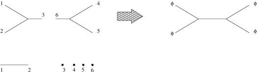
Figure 6: To construct the 4 point diagram we label consecutively the edges of vertices on one hand and propagators and external states on the other. The matrix $K$ corresponds to a permutation which glues them into one diagram.

The matrix $K$ is the block permutation matrix that encodes information on the graph structure of the diagram. The corresponding permutation $\kappa$ connects the external states and propagators to vertices as illustrated for the 4-point diagram in Figure 6. The vertices’ edges which are labeled $1$ through $6$ are connected by permutation to the propagator edges labeled $1$ and $2$ and the external points labeled $3$, $4$, $5$ and $6$. As we can see a suitable choice of a permutation is

$$\kappa:\begin{pmatrix}1&2&3&4&5&6\end{pmatrix}\rightarrow\begin{pmatrix}3&6&1&2&4&5\end{pmatrix},$$ (46)

which corresponds to

$$K=\begin{pmatrix}0\ &0\ &1\ &0\ &0\ &0\ \\ 0\ &0\ &0\ &0\ &0\ &1\ \\ 1\ &0\ &0\ &0\ &0\ &0\ \\ 0\ &1\ &0\ &0\ &0\ &0\ \\ 0\ &0\ &0\ &1\ &0\ &0\ \\ 0\ &0\ &0\ &0\ &1\ &0\ \\ \end{pmatrix}.$$ (47)

For example, multiplying matrices for the 4-point amplitude we find

$$\mathcal{V}\mathcal{P} =({\tilde{V}}^{11})^{2}, \mathcal{X}\mathcal{P} =({\tilde{X}}^{11})^{2},$$ (48)

where

$${\tilde{V}}^{11}_{mn} =\sigma^{\frac{m+n}{2}}V^{11}_{mn}, \tilde{X}^{11}_{mn} =\sigma^{\frac{m+n}{2}}X^{11}_{mn}.$$ (49)

The contribution from the Feynman diagram with 4 external tachyons is given by [39]

$$\frac{e^{-3V_{00}^{11}}g^{2}}{2}\int\prod_{i=1}^{4}(2\pi dw_{i})\phi(w_{i})\delta(\sum w_{i})\\ \int\frac{d\,\sigma}{\sigma^{2}}\operatorname{Det}\left(\frac{1-(\tilde{X}^{11})^{2}}{[1-(\tilde{V}^{11})^{2}]^{13}}\right)\sigma^{-\frac{1}{2}[(w_{1}+w_{2})^{2}+(w_{3}+w_{4})^{2}]}\exp\left(-w_{i}\mathcal{Q}^{ij}w_{j}\right),$$ (50)

with $\mathcal{Q}^{ij}$ defined as

$$\mathcal{Q}^{ij} =\mathcal{U}^{i3}_{0.}\frac{1}{1-(\tilde{V}^{11})^{2}}\tilde{V}^{11}\mathcal{U}^{3j}_{.0}+\mathcal{U}^{ij}_{00} i,j=1,2 \text{ or }i,j=3,4,$$ (51)

$$\mathcal{Q}^{ij} =-\mathcal{U}^{i3}_{0.}\frac{1}{1-(\tilde{V}^{11})^{2}}C\mathcal{U}^{3j}_{.0} (i=1,2\text{ and }j=3,4) \text{ or }(i=3,4\text{ and }j=1,2)$$ (52)

where $\mathcal{U}^{ij}$ is given by

$$\mathcal{U}^{ij}=\begin{pmatrix}V_{00}^{ij}-V_{00}^{i3}-V_{00}^{3j}+V_{00}^{33}&\ \ \tilde{V}_{0n}^{ij}-\tilde{V}_{0n}^{3j}\\ \tilde{V}_{m0}^{ij}-\tilde{V}_{m0}^{i3}&\tilde{V}_{mn}^{ij}\end{pmatrix},$$ (53)

and $C_{mn}=\delta_{mn}(-1)^{n}$. Considering only the contribution coming from level 2 fields, we have to consider only these Neumann coefficients whose powers and products sum up to a total oscillator level of 2, i.e. $V_{01},V_{11},V_{02}$ and $X_{11}$ [57]. Doing so equation (50) simplifies a lot and the integral over the modular parameter reduces to

$$\int d\sigma\sigma^{-\frac{1}{2}\big{[}(w_{1}+w_{2})^{2}+(w_{3}+w_{4})^{2}\big{]}}.$$ (54)

Performing this integral it is easy to get the same result as in formula (9).

Appendix B Construction of $A(w_{1},w_{2},w_{3})$ in the continuous case

Figure 7: Construction of a continuous $A(w_{1},w_{2},w_{3})$: The figure shows the plane $-w_{1}+w_{2}+w_{3}=0$ coincident with the plane of the paper. Dashed lines are the coordinate axes $-w_{1}$, $w_{2}$, $w_{3}$, going at equal angles out of the plane of the paper. The two solid horizontal lines are intersections of the plane $-w_{1}+w_{2}+w_{3}=0$ with the planes $w_{1}=\pm i$. According to (56) the function $A$ is zero along these lines. Clearly, in this projection the cyclic shift of momenta $w_{i}$ corresponds to a 60 degree rotation. Thus, the condition (55) implies that the sum of the values of $A$ over the vertices of any equilateral triangle centered at the origin is one. Together with the reflection symmetry $w_{2}\leftrightarrow w_{3}$ this allows us to fix the value of $A$ at several discrete points. The values are shown on the figure. The slanted solid lines show the locus of the vertices of equilateral triangles with one vertex fixed on the lines $w_{1}^{2}=\pm i$. The assignment of a value for $A$ on one of the slanted lines defines the values on the other line, related by $60^{\circ}$ rotation. These assignments can be made continuously along the lines while taking the values $0$, $1$, and $\frac{1}{2}$ at the symmetrically positioned points. One can then continuously extend $A$ into the rest of the plane, while maintaining (55) by interpolating between the values of $A$ at the boundaries.

As we have discussed in section 4, in order to construct the field redefinition from BSFT to CSFT that preserves general solutions to the equations of motion we need a continuous function $A(w_{1},w_{2},w_{3})$, defined on the plane $-w_{1}+w_{2}+w_{3}=0$ and satisfying

$$A_{2}(w_{1},w_{2},w_{3})+A_{2}(w_{2},w_{3},w_{1})+A_{2}(w_{3},w_{1},w_{2})=1,$$ (55)

and

$$A_{2}(w_{1},w_{2},w_{3})|_{w_{1}^{2}=-1}=0.$$ (56)

Figure 7 illustrates the construction of the desired function.

References

- [1] A. Sen, “Universality of the tachyon potential,” JHEP 9912, 027 (1999) hep-th/9911116.
- [2] E. Witten, “Noncommutative Geometry And String Field Theory,” Nucl. Phys. B 268, 253 (1986).
- [3] W. Taylor and B. Zwiebach, “D-branes, tachyons, and string field theory,” hep-th/0311017.
- [4] A. Sen, “Tachyon dynamics in open string theory,” hep-th/0410103.
- [5] E. Witten, “On background independent open string field theory,” Phys. Rev. D 46, 5467 (1992) hep-th/9208027.
- [6] E. Witten, “Some computations in background independent off-shell string theory,” Phys. Rev. D 47, 3405 (1993) hep-th/9210065.
- [7] S. L. Shatashvili, “Comment on the background independent open string theory,” Phys. Lett. B 311, 83 (1993) hep-th/9303143.
- [8] S. L. Shatashvili, “On the problems with background independence in string theory,” Alg. Anal. 6, 215 (1994) hep-th/9311177.
- [9] A. Sen, “Rolling tachyon,” JHEP 0204, 048 (2002) hep-th/0203211.
- [10] A. Sen, “Tachyon matter,” JHEP 0207, 065 (2002) hep-th/0203265.
- [11] A. Sen,“Field theory of tachyon matter,” Mod. Phys. Lett. A 17, 1797 (2002) hep-th/0204143.
- [12] S. Sugimoto and S. Terashima, “Tachyon matter in boundary string field theory,” JHEP 0207, 025 (2002) hep-th/0205085.
- [13] J. A. Minahan, “Rolling the tachyon in super BSFT,” JHEP 0207, 030 (2002) hep-th/0205098.
- [14] A. Sen, “Time evolution in open string theory,” JHEP 0210, 003 (2002) hep-th/0207105.
- [15] A. Sen, “Time and tachyon,” Int. J. Mod. Phys. A 18, 4869 (2003) hep-th/0209122.
- [16] F. Larsen, A. Naqvi and S. Terashima, “Rolling tachyons and decaying branes,” JHEP 0302, 039 (2003) hep-th/0212248.
- [17] C. G. Callan and I. R. Klebanov, “Exact C = 1 boundary conformal field theories,” Phys. Rev. Lett. 72, 1968 (1994) hep-th/9311092.
- [18] C. G. Callan, I. R. Klebanov, A. W. W. Ludwig and J. M. Maldacena, “Exact solution of a boundary conformal field theory,” Nucl. Phys. B 422, 417 (1994) hep-th/9402113.
- [19] J. Polchinski and L. Thorlacius, “Free fermion representation of a boundary conformal field theory,” Phys. Rev. D 50, 622 (1994) hep-th/9404008.
- [20] A. Sen, “Dirac-Born-Infeld action on the tachyon kink and vortex,” Phys. Rev. D 68, 066008 (2003) hep-th/0303057.
- [21] D. Kutasov and V. Niarchos, “Tachyon effective actions in open string theory,” Nucl. Phys. B 666, 56 (2003) hep-th/0304045.
- [22] M. R. Garousi, “Slowly varying tachyon and tachyon potential,” JHEP 0305, 058 (2003) hep-th/0304145.
- [23] A. Fotopoulos and A. A. Tseytlin, “On open superstring partition function in inhomogeneous rolling tachyon background,” JHEP 0312, 025 (2003) hep-th/0310253.
- [24] A. Strominger, “Open string creation by S-branes,” hep-th/0209090.
- [25] M. Gutperle and A. Strominger, “Timelike boundary Liouville theory,” Phys. Rev. D 67, 126002 (2003) hep-th/0301038.
- [26] F. Leblond and A. W. Peet, “SD-brane gravity fields and rolling tachyons,” JHEP 0304, 048 (2003) hep-th/0303035.
- [27] A. Strominger and T. Takayanagi, “Correlators in timelike bulk Liouville theory,” Adv. Theor. Math. Phys. 7, 369 (2003) hep-th/0303221.
- [28] V. Schomerus, “Rolling tachyons from Liouville theory,” JHEP 0311, 043 (2003) hep-th/0306026.
- [29] J. McGreevy and H. Verlinde, “Strings from tachyons: The c = 1 matrix reloaded,” JHEP 0312, 054 (2003) hep-th/0304224.
- [30] I. R. Klebanov, J. Maldacena and N. Seiberg, “D-brane decay in two-dimensional string theory,” JHEP 0307, 045 (2003) hep-th/0305159.
- [31] N. R. Constable and F. Larsen, “The rolling tachyon as a matrix model,” JHEP 0306, 017 (2003) hep-th/0305177.
- [32] J. McGreevy, J. Teschner and H. Verlinde, “Classical and quantum D-branes in 2D string theory,” JHEP 0401, 039 (2004) hep-th/0305194.
- [33] T. Takayanagi and N. Toumbas, “A matrix model dual of type 0B string theory in two dimensions,” JHEP 0307, 064 (2003) hep-th/0307083.
- [34] M. R. Douglas, I. R. Klebanov, D. Kutasov, J. Maldacena, E. Martinec and N. Seiberg, “A new hat for the c = 1 matrix model,” hep-th/0307195.
- [35] T. Lee and G. W. Semenoff, “Fermion representation of the rolling tachyon boundary conformal field theory,” hep-th/0502236.
- [36] N. Moeller and B. Zwiebach, “Dynamics with infinitely many time derivatives and rolling tachyons,” JHEP 0210, 034 (2002) hep-th/0207107.
- [37] M. Fujita and H. Hata, “Time dependent solution in cubic string field theory,” JHEP 0305, 043 (2003) hep-th/0304163.
- [38] D. Ghoshal and A. Sen, “Gauge and general coordinate invariance in nonpolynomial closed string theory,” Nucl. Phys. B 380, 103 (1992) hep-th/9110038.
- [39] E. Coletti, I. Sigalov and W. Taylor, “Abelian and nonabelian vector field effective actions from string field theory,” JHEP 0309, 050 (2003) hep-th/0306041.
- [40] J. Kluson, “Time dependent solution in open bosonic string field theory,” hep-th/0208028.
- [41] T. G. Erler and D. J. Gross, “Locality, causality, and an initial value formulation for open string field hep-th/0406199.
- [42] T. G. Erler, “Level truncation and rolling the tachyon in the lightcone basis for open string field theory,” hep-th/0409179.
- [43] I. Y. Aref’eva, L. V. Joukovskaya and A. S. Koshelev, “Time evolution in superstring field theory on non-BPS brane. I: Rolling tachyon and energy-momentum conservation,” JHEP 0309, 012 (2003) hep-th/0301137.
- [44] H. t. Yang, “Stress tensors in p-adic string theory and truncated OSFT,” JHEP 0211, 007 (2002) hep-th/0209197.
- [45] N. Moeller and M. Schnabl, “Tachyon condensation in open-closed p-adic string theory,” JHEP 0401, 011 (2004) hep-th/0304213.
- [46] K. Ohmori, “Toward open-closed string theoretical description of rolling tachyon,” Phys. Rev. D 69, 026008 (2004) hep-th/0306096.
- [47] M. Fujita and H. Hata, “Rolling tachyon solution in vacuum string field theory,” Phys. Rev. D 70, 086010 (2004) hep-th/0403031.
- [48] L. Bonora, C. Maccaferri, R. J. Scherer Santos and D. D. Tolla, “Exact time-localized solutions in vacuum string field theory,” hep-th/0409063.
- [49] T. Okuda and S. Sugimoto, “Coupling of rolling tachyon to closed strings,” Nucl. Phys. B 647, 101 (2002) [arXiv:hep-th/0208196].
- [50] N. Lambert, H. Liu and J. Maldacena, “Closed strings from decaying D-branes,” arXiv:hep-th/0303139.
- [51] J. Shelton, “Closed superstring emission from rolling tachyon backgrounds,” JHEP 0501, 037 (2005) [arXiv:hep-th/0411040].
- [52] V. Forini, G. Grignani and G. Nardelli, “A new rolling tachyon solution of cubic string field theory,” hep-th/0502151.
- [53] L. Brekke, P. G. Freund, M. Olson and E. Witten, “Nonarchimedean String Dynamics,” Nucl. Phys. B 302, 365 (1988).
- [54] Y. Volovich, “Numerical study of nonlinear equations with infinite number of derivatives,” J. Phys. A 36, 8685 (2003) math-ph/0301028.
- [55] V. S. Vladimirov and Y. I. Volovich, “On the nonlinear dynamical equation in the p-adic string theory,” math-ph/0306018.
- [56] J. Gomis, K. Kamimura and T. Ramirez, “Physical reduced phase space of non-local theories,” Nucl. Phys. B 696, 263 (2004) [arXiv:hep-th/0311184].
- [57] W. Taylor, “Perturbative diagrams in string field theory,” hep-th/0207132.
- [58] A. Sen and B. Zwiebach, “Tachyon condensation in string field theory,” JHEP 0003, 002 (2000) [arXiv:hep-th/9912249].
- [59] N. Moeller and W. Taylor, “Level truncation and the tachyon in open bosonic string field theory,” Nucl. Phys. B 583, 105 (2000) hep-th/0002237.
- [60] I. Ellwood and W. Taylor, “Gauge invariance and tachyon condensation in open string field theory,” hep-th/0105156.
- [61] W. Taylor, “A perturbative analysis of tachyon condensation,” JHEP 0303, 029 (2003) hep-th/0208149.
- [62] J. R. David, “U(1) gauge invariance from open string field theory,” JHEP 0010, 017 (2000) hep-th/0005085.
- [63] E. Coletti, V. Forini, G. Grignani, G. Nardelli and M. Orselli, “Exact potential and scattering amplitudes from the tachyon non-linear beta-function,” JHEP 0403, 030 (2004) hep-th/0402167.
- [64] K. Hashimoto and S. Terashima, “Boundary string field theory as a field theory: Mass spectrum and interaction,” JHEP 0410, 040 (2004) hep-th/0408094.
- [65] A. Sen and B. Zwiebach, “Large marginal deformations in string field theory,” JHEP 0010, 009 (2000) hep-th/0007153.
- [66] I. Ellwood and W. Taylor, “Open string field theory without open strings,” Phys. Lett. B 512, 181 (2001) hep-th/0103085.
- [67] W. Taylor, “Perturbative computations in string field theory,” hep-th/0404102.