hep-th/0505029

NSF-KITP-05-27

Supersymmetry Breaking from a Calabi-Yau Singularity

D. Berenstein^∗, C. P. Herzog^†, P. Ouyang^∗, and S. Pinansky^∗
${\dagger}$ Kavli Institute for Theoretical Physics University of California Santa Barbara, CA 93106, USA $*$ Physics Department University of California Santa Barbara, CA 93106, USA

We conjecture a geometric criterion for determining whether supersymmetry is spontaneously broken in certain string backgrounds. These backgrounds contain wrapped branes at Calabi-Yau singularites with obstructions to deformation of the complex structure. We motivate our conjecture with a particular example: the $Y^{2,1}$ quiver gauge theory corresponding to a cone over the first del Pezzo surface, $dP_{1}$. This setup can be analyzed using ordinary supersymmetric field theory methods, where we find that gaugino condensation drives a deformation of the chiral ring which has no solutions. We expect this breaking to be a general feature of any theory of branes at a singularity with a smaller number of possible deformations than independent anomaly-free fractional branes.

May 2005

1 Introduction

Supersymmetry and supersymmetry breaking are central ideas both in contemporary particle physics and in mathematical physics. In this paper, we argue that for a large new class of D-brane models there exists a simple geometric criterion which determines whether supersymmetry breaking occurs.

The models of interest are based on Calabi-Yau singularities with D-branes placed at or near the singularity. By taking a large volume limit, it is possible to decouple gravity from the theory, and ignore the Calabi-Yau geometry far from the branes. Although one typically begins the construction with branes free to move throughout the Calabi-Yau space, many interesting theories include fractional branes (or wrapped branes), which are D-branes stuck at the singularity and which cannot move away from it. These fractional branes can lead to topology changes in the geometry via gaugino condensation, which can be understood in terms of deformations of the complex structure of the Calabi-Yau singularity, and result in the replacement of branes by fluxes [1, 2]. Models of this type, Calabi-Yau geometries with fluxes, are among the ingredients used to construct viable cosmological models within string theory with a positive cosmological constant [3], and which, because of that positivity, ultimately break supersymmetry. With current approaches in the literature, the issue of whether or not supersymmetry breaking is under control is controversial.

It turns out that there exist some singular geometries which admit fractional branes, but for which the associated complex structure deformations are obstructed. We will argue that in such setups a deformation can still take place, but that the geometric obstruction induces supersymmetry breaking.

Conjecture.

Given a set of ordinary and fractional branes probing a Calabi-Yau singularity, supersymmetry breaking by obstructed geometry (SUSY-BOG) occurs when the singularity admits fewer deformations than the number of (anomaly free) independent fractional branes that one can add to the system.

In this paper we will show how this breaking occurs in one particular example, D-branes probing the singularity of the Calabi-Yau cone over the first del Pezzo surface, $dP_{1}$. This case can be analyzed using the gauge theory/gravity correspondence. In field theory, the mechanism that spontaneously breaks SUSY is simply gaugino condensation. In terms of the dual gravity theory and its local Calabi-Yau geometry, the deformation obstruction causes the breaking. The SUSY-BOG adds a new feature to the string theory landscape.

$dP_{1}$ belongs to a large class of singularities for which this geometric obstruction is easy to understand. We need the technical concept from algebraic geometry of a singularity which is an “incomplete intersection variety.” These varieties are described by $n$ equations in $m$ variables, where the dimension of the variety is strictly greater than $m-n$. Although the $n$ equations or relations are redundant, it is impossible to reduce the number of equations further without changing the geometry. In the case of an incomplete intersection, the redundancy makes it hard to deform the equations consistently, giving an obstruction to deformation. These incomplete intersections are believed to be more generic than “complete intersections,” where the dimension of the variety is equal to $m-n$.

In the dual field theory, the $m$ complex variables can be associated to generators of the chiral ring of the theory, while the relations in the geometry can be understood as relations in the chiral ring. We will develop this picture further to make this set of ideas more precise. A generic property of fractional branes is that they have gaugino condensation on their worldvolume, which translates to non-trivial deformed relations in the chiral ring of the field theory. When it is possible to deform the equations of the chiral ring consistently, the field theory realizes a supersymmetric vacuum. If it is impossible to deform the equations in the chiral ring consistently, then the theory spontaneously breaks supersymmetry.

1.1 The Conifold vs. $dP_{1}$

Perhaps the prototypical example of a Calabi-Yau singularity with fractional branes is the conifold singularity, in the setups of Klebanov and Witten [4] (see also [5, 6]), and its generalization to the warped deformed conifold geometry of Klebanov and Strassler (KS) [1]. The KS solution is an example of a space with no obstruction to deformation, and in this case chiral symmetry breaking and confinement in the strongly coupled dual gauge theory may be identified with the deformation in a precise way.

Recall that the construction of the KS solution begins by placing a stack of $N$ D3-branes and $M$ D5-branes at the tip of the conifold:

$$\sum_{i=1}^{4}z_{i}^{2}=0\ .$$ (1)

The D5-branes are fractional. In the supergravity solution, the D-branes are replaced by their corresponding RR five-form and three-form fluxes. The three-form flux from the D5-branes leads to a singularity unless the conifold is deformed:

$$\sum_{i=1}^{4}z_{i}^{2}=\epsilon\ .$$ (2)

This $\epsilon$ parameter is interpreted as a gaugino condensate in the dual theory and breaks the R-symmetry to ${\mathbb{Z}}_{2}$. Moreover, cutting off the cone at a radius $\epsilon$ produces confining behavior of strings in this geometry which are dual to electric flux tubes in the gauge theory.

Naively, one could imagine that a very similar phenomenon occurs for the cone over $dP_{1}$, but there is an obstruction. A theorem by Altmann [7] claims that there are no deformations of this cone. While the conifold has the single defining equation (1), we recall below that the cone over $dP_{1}$ requires twenty algebraic relations in ${\mathbb{C}}^{9}$ which are not all independent. It is impossible to alter all twenty consistently by adding the analog of $\epsilon$ in (2).

The conformal analog of the $dP_{1}$ model with no D5-branes was first proposed separately by Kehagias [6] and by Morrison and Plesser [5] as an example of a generalized AdS/CFT correspondence. Type IIB string theory propagating in $AdS_{5}\times Y$, where $Y$ is a particular U(1) bundle over $dP_{1}$, is equivalent to a superconformal ${\mathcal{N}}=1$ gauge theory whose field content and superpotential were later derived in [8] using techniques from toric geometry (see Fig. 1).

Recently, the metric on $Y$ was discovered. Martelli and Sparks [9] have shown that this U(1) bundle over $dP_{1}$, $Y=Y^{2,1}$, is a particular example of the $Y^{p,q}$ Sasaki-Einstein manifolds found in [10, 11]. Using the explicit metric, impressive comparisons of the conformal anomaly coefficients and R-charges between the AdS and the CFT sides were carried out for $dP_{1}$ in [12, 13].

As was the case for the conifold, adding D5-branes to the tip of the cone over $dP_{1}$ breaks conformal invariance and leads to a cascading gauge theory [14, 15]. Recently, a supergravity solution dual to this cascading theory was derived by Herzog, Ejaz, and Klebanov (HEK) [16]. The HEK solution shares many of the features of the predecessor of the KS solution, the Klebanov-Tseytlin (KT) solution [17]. Like the KT solution, the HEK solution is singular in the infrared (small radius); at large radius, in the ultraviolet, the KT solution approaches the KS solution. The large radius region can be used to calculate geometrically the NSVZ beta functions and logarithmic running in the number of colors, and this geometric behavior matches our field theoretic understanding of a duality cascade.

However, there currently is no known analog of the KS solution for $dP_{1}$ that smooths the singularity in the infrared. The motivation behind this research was to understand the infrared physics of $dP_{1}$.

1.2 Summary of the $dP_{1}$ Argument

Since the Calabi-Yau deformations are obstructed, we argue that supersymmetry is broken at the bottom of the duality cascade for $dP_{1}$. Our argument has three field theoretic legs. First we argue that there is no superconformal fixed point to which the cascading theory may flow, ruling out strong coupling behavior that is not confinement. Next, turning on Fayet-Iliopoulos terms in the field theory, we show that the theory should confine in the infrared. Last, using the Konishi anomaly [18], we show there are no solutions to the F-term equations.

The last step requires some immediate clarification. The field theory analysis is well suited for studying vacua where mesonic operators get expectation values – the mesonic branch – and is less so for the baryonic branch. We will show that the mesonic branch of the $dP_{1}$ field theory spontaneously breaks supersymmetry.

We have a traditional field theory argument that supersymmetry is not preserved along the baryonic branch, but the argument is not as rigorous as the Konishi anomaly approach. It may be that there exists a supersymmetric, pure flux supergravity solution (which does not involve a Calabi-Yau manifold), similar to the recent $SU(3)$ structure solutions of [19, 20]. Recall that the KS solution represents a particular point in the baryonic branch of the conifold field theory [21]. As one moves along the baryonic branch, one finds that the geometry is no longer Calabi-Yau but is instead an $SU(3)$ structure solution where probe D3-branes break supersymmetry.

For generic initial number of D3- and D5-branes in the UV, we expect to have left-over D3-branes at the bottom of the cascade. The KS solution represents a particular point in the baryonic branch where these D3-branes will remain supersymmetric. However, even if there is an $SU(3)$ structure solution for $dP_{1}$, the left-over D3-branes will always break supersymmetry.

We emphasize that the supersymmetry breaking is an infrared effect. The warp factor in the geometry will lead to an exponential separation between the ultraviolet and infrared scales, giving a natural way of achieving low-scale supersymmetry breaking should we embed this cone over $dP_{1}$ in a compact Calabi-Yau. An optimistic point of view is that one might be able to build supergravity solutions from compactified versions of this cone over $dP_{1}$, and using these solutions, produce realistic cosmological models similar to [3] where all stringy moduli are stabilized and supersymmetry is broken in a controlled way. Such solutions deserve further study.

2 The Gauge Theory for $dP_{1}$

The quiver theory for the first del Pezzo has four gauge groups and a number of bifundamental fields conveniently summarized using a quiver diagram (see Fig. 1).

Figure 1: The quiver theory for $Y^{2,1}$, also known as an irregular $U(1)$ fibration of ${\mathbb{P}}^{2}$ blown up at a point.

The superpotential for the first del Pezzo takes the form

$$W=\epsilon_{\alpha\beta}U_{L}^{\alpha}V^{\beta}Y_{1}-\epsilon_{\alpha\beta}U_{R}^{\alpha}Y_{2}V^{\beta}-\epsilon_{\alpha\beta}U_{L}^{\alpha}Y_{3}U_{R}^{\beta}Z\ .$$ (3)

There is an $SU(2)$ global symmetry: the indices $\alpha$ and $\beta$ are either one or two and $\epsilon_{12}=1$.

In the case $M=0$, the gauge theory has a superconformal fixed point with an AdS/CFT dual description: type IIB string theory in a $AdS_{5}\times Y^{2,1}$ background. Adding $M$ D5-branes breaks the superconformal symmetry and starts a Seiberg duality cascade, as argued in [14, 15, 16]. In the limit $M\ll N$, we can calculate the NSVZ $\beta$-functions and find that generically the $SU(N+3M)$ group runs to strong coupling first as the energy scale decreases. Taking the Seiberg dual of the $SU(N+3M)$ group yields the same quiver and superpotential but with $N\to N-M$, i.e. the number of D3-branes slowly decreases with energy scale.

Before tackling the problem of what happens when $N$ becomes of order $M$, we would like to demonstrate how the geometry of the first del Pezzo can be recovered from the F-term relations of this gauge theory.

2.1 The Chiral Ring

The superpotential (3) gives rise to the ten classical F-term equations

$$\frac{\partial W}{\partial X_{i}}=0\ ,$$ (4)

one for each $X_{i}$, where $X_{i}=U_{L}^{\alpha}$, $U_{R}^{\alpha}$, $V^{\alpha}$, $Y_{j}$, or $Z$. We list these ten equations:

$$U_{L}^{1}V^{2} = U_{L}^{2}V^{1}\ ,$$ (5)

$$V^{1}U_{R}^{2} = V^{2}U_{R}^{1}\ ,$$ (6)

$$U_{R}^{1}ZU_{L}^{2} = U_{R}^{2}ZU_{L}^{1}\ ,$$ (7)

$$U_{L}^{1}Y_{3}U_{R}^{2} = U_{L}^{2}Y_{3}U_{R}^{1}\ ,$$ (8)

$$V^{\beta}Y_{1} = Y_{3}U_{R}^{\beta}Z\ ,$$ (9)

$$Y_{2}V^{\beta} = ZU_{L}^{\beta}Y_{3}\ ,$$ (10)

$$Y_{1}U_{L}^{\beta} = U_{R}^{\beta}Y_{2}\ .$$ (11)

To see the geometry emerge from the F-term equations, we study the spectrum of chiral primary operators of the schematic form

$${\mathcal{O}}=\mbox{tr}\left(X_{i_{1}}X_{i_{2}}X_{i_{3}}\ldots X_{i_{n}}\right)\ ,$$ (12)

where we contract all of the color indices to form a gauge invariant operator. The trace structure means that these gauge invariant operators will correspond to loops in the quiver diagram.

The reason this expression (12) is schematic is that the actual chiral primary operator will be a polynomial of such traces. The traces generate the chiral ring. Just as we think of harmonic forms as representatives of classes in cohomology, we can think of a chiral primary operator as a representative of a class of operators related by the F-term equations. By only giving a single trace, we are really specifying a class of such operators related to each other by the F-term equations.

There are six types of operators that loop just once around the quiver

$$U_{R}^{\alpha}Y_{2}Y_{3}\;;\;\;\;U_{R}^{\alpha}Y_{2}V^{\beta}\;;\;\;\;Y_{1}U_{L}^{\alpha}Y_{3}\;;\;\;\;Y_{1}U_{L}^{\alpha}V^{\beta}\;;\;\;\;$$

$$U_{R}^{\alpha}ZU_{L}^{\beta}Y_{3}\;;\;\;\;U_{R}^{\alpha}ZU_{L}^{\beta}V^{\gamma}\ .$$ (13)

From these six building blocks, we can form any operator of the form (12). The final trace will always be over the gauge group in the lower right hand corner of the quiver.

Now of these six building blocks, only three are independent. Note that from (11), $U_{R}^{\alpha}Y_{2}Y_{3}=Y_{1}U_{L}^{\alpha}Y_{3}$ and that $U_{R}^{\alpha}Y_{2}V^{\beta}=Y_{1}U_{L}^{\alpha}V^{\beta}$. Moreover, under (10), $U_{R}^{\alpha}Y_{2}V^{\beta}=U_{R}^{\alpha}ZU_{L}^{\beta}Y_{3}$. We will choose the three independent blocks

$$U_{R}^{\alpha}Y_{2}Y_{3}\;;\;\;\;U_{R}^{\alpha}ZU_{L}^{\beta}Y_{3}\;;\;\;\;U_{R}^{\alpha}ZU_{L}^{\beta}V^{\gamma}\ .$$ (14)

These blocks satisfy some additional important relations. They are symmetric under interchange of their $SU(2)$ indices. From (7), we see that $U_{R}^{\alpha}ZU_{L}^{\beta}Y_{3}=U_{R}^{\beta}ZU_{L}^{\alpha}Y_{3}$. Moreover, from (7) and (5), we see that

$$U_{R}^{\alpha}ZU_{L}^{\beta}V^{\gamma}=U_{R}^{\alpha}ZU_{L}^{\gamma}V^{\beta}=U_{R}^{\gamma}ZU_{L}^{\alpha}V^{\beta}\ .$$ (15)

We now study what happens when we assemble these blocks into larger operators. We find that

$$U_{R}^{\alpha}Y_{2}Y_{3}\cdot U_{R}^{\beta}ZU_{L}^{\gamma}V^{\delta} = U_{R}^{\alpha}Y_{2}V^{\beta}Y_{1}U_{L}^{\gamma}V^{\delta}$$

$$= U_{R}^{\alpha}ZU_{L}^{\beta}Y_{3}U_{R}^{\gamma}Y_{2}V^{\delta}$$

$$= U_{R}^{\alpha}ZU_{L}^{\beta}Y_{3}\cdot U_{R}^{\gamma}ZU_{L}^{\delta}Y_{3}\ .$$

The $\cdot$ has been added as a guide to the eye. Similar types of manipulation reveal also that these blocks commute with one another. In particular

$$U_{R}^{\alpha}Y_{2}Y_{3}\cdot U_{R}^{\beta}ZU_{L}^{\gamma}Y_{3}=U_{R}^{\beta}ZU_{L}^{\gamma}Y_{3}\cdot U_{R}^{\alpha}Y_{2}Y_{3}\ ,$$ (17)

and that

$$U_{R}^{\alpha}ZU_{L}^{\beta}Y_{3}\cdot U_{R}^{\gamma}ZU_{L}^{\delta}V^{\epsilon}=U_{R}^{\gamma}ZU_{L}^{\delta}V^{\epsilon}\cdot U_{R}^{\alpha}ZU_{L}^{\beta}Y_{3}\ .$$ (18)

Finally, with a little more work, one can show that any product of the (14) is symmetric in the $SU(2)$ indices.

From these assembled facts, we conclude that the most general operator of the form (12) takes the schematic form

$$\mbox{tr}\left(\prod_{i=1}^{n}(U_{R}^{\alpha_{i}}ZU_{L}^{\beta_{i}}Y_{3})\prod_{j=1}^{m}(U_{R}^{\gamma_{j}}Y_{2}Y_{3})\right)$$ (19)

or

$$\mbox{tr}\left(\prod_{i=1}^{n}(U_{R}^{\alpha_{i}}ZU_{L}^{\beta_{i}}Y_{3})\prod_{j=1}^{m}(U_{R}^{\gamma_{j}}ZU_{L}^{\delta_{j}}V^{\epsilon_{j}})\right)\ .$$ (20)

These operators are understood to be totally symmetric in the $SU(2)$ indices. The first operator transforms in a $2n+m+1$ dimensional representation of $SU(2)$ while the second transforms in a $2n+3m+1$ dimensional representation.

At this point, it is convenient to introduce some new notation for the building blocks (14):

$$\begin{array}[]{ccc}\left.\begin{array}[]{c}a_{1}=U_{R}^{1}Y_{2}Y_{3}\\ a_{2}=U_{R}^{2}Y_{2}Y_{3}\end{array}\right.,&\left.\begin{array}[]{c}b_{1}=U_{R}^{1}ZU_{L}^{1}Y_{3}\\ b_{2}=U_{R}^{1}ZU_{L}^{2}Y_{3}\\ b_{3}=U_{R}^{2}ZU_{L}^{2}Y_{3}\end{array}\right.,&\left.\begin{array}[]{c}c_{1}=U_{R}^{1}ZU_{L}^{1}V^{1}\\ c_{2}=U_{R}^{1}ZU_{L}^{1}V^{2}\\ c_{3}=U_{R}^{1}ZU_{L}^{2}V^{2}\\ c_{4}=U_{R}^{2}ZU_{L}^{2}V^{2}\end{array}\right..\end{array}$$ (21)

From these nine operators, which we can treat as commuting, we can construct any operator of the form (19) or (20) subject to some relations. In particular, we know that the resulting operator must be totally symmetric in the $SU(2)$ indices and moreover an $a$ and $c$ type operator annihilate to form two $b$ operators (2.1). The set of twenty relations these operators satisfy is given in Appendix A.

We can find a set of monomials with identical algebraic properties. In particular, we let $x$, $y$, $z\in{\mathbb{C}}$ and

$$\begin{array}[]{ccc}\begin{array}[]{c}a_{1}=x^{2}y\\ a_{2}=x^{2}z\end{array},\begin{array}[]{c}b_{1}=xy^{2}\\ b_{2}=xyz\\ b_{3}=xz^{2}\end{array},\begin{array}[]{l}c_{1}=y^{3}\\ c_{2}=y^{2}z\\ c_{3}=yz^{2}\\ c_{4}=z^{3}\end{array}.\end{array}$$ (22)

In this way, the operators commute by construction and the number of $x$’s labels whether the operator is of type $a$, $b$, or $c$. The number of $y$’s equals the number of $SU(2)$ indices set to one while the number of $z$’s equals the number of $SU(2)$ indices set to two. In any product of the $a$, $b$, and $c$, the fact that the $x$, $y$, and $z$ commute is equivalent to the fact that the operator is totally symmetric in the $SU(2)$ indices. Only slightly more difficult to see is (2.1).

Because the $a_{i}$, $b_{j}$ and $c_{k}$ commute, one can diagonalize all of these matrix valued operators simultaneously. Eigenvalue by eigenvalue, these operators describe a three dimensional variety, parametrized above by $x,y,z$. This variety is the Calabi-Yau geometry we are interested in. The description of a general point in the moduli space is a set of $N$ unordered points of the Calabi-Yau geometry. We call this moduli space the mesonic branch of the theory. That we have found a Calabi-Yau in this way is in line with the expectations of reverse geometric engineering [22].

Now, treating $x$, $y$, and $z$ as homogenous coordinates on ${\mathbb{P}}^{2}$, this set of monomials can be reinterpreted as a set of linearly independent polynomials on ${\mathbb{P}}^{2}$ which vanish at the point $(1,0,0)\sim(\lambda,0,0)$ for $\lambda\in{\mathbb{C}}^{*}$. This set of monomials then provides a map from ${\mathbb{P}}^{2}\to{\mathbb{P}}^{8}$ with the point $(1,0,0)$ missing because the origin is not contained in ${\mathbb{P}}^{8}$. The smallest surface containing the image of this map is well known to be the first del Pezzo, or ${\mathbb{P}}^{2}$ blown up at a point.

2.2 The First del Pezzo

We can be more precise in our description of this first del Pezzo. It is easy to embed ${\mathbb{P}}^{2}$ blown up at a point inside ${\mathbb{P}}^{2}\times{\mathbb{P}}^{1}$. Let $x$, $y$, and $z$ be homogenous coordinates on the ${\mathbb{P}}^{2}$, as above, and let $w_{1}$ and $w_{2}$ be coordinates on the ${\mathbb{P}}^{1}$. The first del Pezzo is described as the hypersurface $dP_{1}\subset{\mathbb{P}}^{2}\times{\mathbb{P}}^{1}$ satisfying $yw_{2}=zw_{1}$.

We now construct a map from ${\mathbb{P}}^{2}\times{\mathbb{P}}^{1}$ to ${\mathbb{P}}^{11}$ by considering all monomials linear in the $w_{i}$ and quadratic in the $x$, $y$, and $z$. (Algebraic geometers would call this map a composition of the Segre and Veronese maps.)

$${\mathbb{P}}^{2}\times{\mathbb{P}}^{1} \longrightarrow {\mathbb{P}}^{11}$$

$$(x,y,z;w_{1},w_{2}) \longmapsto (x^{2}w_{1},xyw_{1},xzw_{1},y^{2}w_{1},yzw_{1},z^{2}w_{1},$$

$$\;x^{2}w_{2},xyw_{2},xzw_{2},y^{2}w_{2},yzw_{2},z^{2}w_{2})$$

This map restricts to an injective map from $dP_{1}$ to ${\mathbb{P}}^{8}$ by requiring $yw_{2}=zw_{1}$ – of the twelve monomials above, only nine are linearly independent under this relation.

Now for a point on $dP_{1}$ where $y$ and $z$ do not both vanish, the constraint $yw_{2}=zw_{1}$ fixes a point on the ${\mathbb{P}}^{1}$ which we can take to be $w_{2}=z$ and $w_{1}=y$. In this case, the twelve monomials in ${\mathbb{P}}^{11}$ reduce precisely to the nine monomials given as (22). Thus this $dP_{1}\subset{\mathbb{P}}^{8}$ certainly contains the image of the map described above from ${\mathbb{P}}^{2}\to{\mathbb{P}}^{8}$.

Using the twelve monomials that depend on the $w_{i}$, we can also describe the extra blown up ${\mathbb{P}}^{1}$ in $dP_{1}$. Consider the case $y=0$ and $z=0$. Now, the $w_{i}$ are unconstrained, and the only two nonvanishing monomials in the ${\mathbb{P}}^{11}$ are $x^{2}w_{1}$ and $x^{2}w_{2}$, which parametrize the blown up ${\mathbb{P}}^{1}$.

Naively, this description of the first del Pezzo seems overly complicated. For example, we may just as easily consider the simpler Segre map to ${\mathbb{P}}^{5}$:

$${\mathbb{P}}^{2}\times{\mathbb{P}}^{1} \longrightarrow {\mathbb{P}}^{5}$$

$$(x,y,z;w_{1},w_{2}) \longmapsto (xw_{1},yw_{1},zw_{1},xw_{2},yw_{2},zw_{2})$$

Subject to the relation $yw_{2}=zw_{1}$ we have a simpler embedding of the first del Pezzo inside ${\mathbb{P}}^{4}$. However, we are not just describing the geometry of the Del-Pezzo surface, but a particular algebraic cone over it, which results from blowing down the zero section of the total space of a line bundle over $dP_{1}$ which makes the space a Calabi-Yau geometry.

3 D5-branes and Superconformal Fixed Points

We will now give a plausible argument that the field theory on a stack of D3-branes and D5-branes probing a $dP_{1}$ singularity does not have a superconformal fixed point in the infrared. This absence helps rule out strong coupling behaviors in the IR field theory which are not gaugino condensation.

A necessary condition for the presence of a superconformal fixed point in a gauge theory is the vanishing of the NSVZ beta functions and the requirement that the superpotential be marginal. We will assume that there is an $SU(2)$ global symmetry. As a result, the anomalous dimensions of the doublet fields will be equal, $\gamma_{V^{1}}=\gamma_{V^{2}}$ and similarly for the $U_{L}$ and $U_{R}$. Moreover, because of this $SU(2)$, there will only be three independent superpotential couplings.

We find it convenient to work with R-charges rather than with the anomalous dimensions $\gamma$. Recall that at a superconformal fixed point, the supersymmetry algebra implies that $3R=2+\gamma$.

For the NSVZ beta functions to vanish, the following expressions must vanish:

$$\beta_{0} = 2N+(N+3M)(R_{Z}-1)+(N+M)(R_{Y_{1}}-1)+2(N+2M)(R_{U_{L}}-1)\ ,$$

$$\beta_{1} = 2(N+M)+(N+2M)(R_{Y_{3}}-1)+2(N+2M)(R_{V}-1)+$$

$$N(R_{Y_{1}}-1)+2(N+3M)(R_{U_{R}}-1)\ ,$$

$$\beta_{2} = 2(N+2M)+(N+M)(R_{Y_{3}}-1)+2(N+M)(R_{V}-1)+$$

$$(N+3M)(R_{Y_{2}}-1)+2N(R_{U_{L}}-1)\ ,$$

$$\beta_{3} = 2(N+3M)+N(R_{Z}-1)+(N+2M)(R_{Y_{2}}-1)+2(N+M)(R_{U_{R}}-1)\ .$$

Moreover, the superpotential couplings must be marginal, which implies that each of the $b_{i}$ have R-charge two:

$$2 = R_{U_{L}}+R_{Y_{1}}+R_{V}\,$$

$$2 = R_{U_{R}}+R_{Y_{2}}+R_{V}\ ,$$

$$2 = R_{Z}+R_{U_{R}}+R_{Y_{3}}+R_{U_{L}}\ .$$

This set of seven equations is not linearly independent. In the case $M=0$, there is a two parameter family of solutions. In the case $M\neq 0$, there is just a one parameter family.

However, the existence of a family of solutions to these beta function constraints is not sufficient to guarantee the existence of a superconformal fixed point. From Intriligator and Wecht [23], we know that at a superconformal fixed point, the conformal anomaly $a\sim{\mbox{T}r}R^{3}$ should be at a local maximum. Here, ${\mbox{T}r}R^{3}$ is a trace over the R-charges of all of the fermions in the gauge theory. For the $M=0$ case, it is indeed possible to maximize $a$ over the two parameter family of solutions, and one can match the results to geometric expectations [9, 12, 13]. However, in the case $M\neq 0$, $a$ cannot be maximized. If we let $R_{V}$ parametrize the family of solutions to the beta function constraints, it is straightforward to see that

$$\mbox{tr}R^{3}=24(-19M^{2}-27MN-9N^{2}+(M+N)(2M+N)R_{V})$$ (23)

is a linear function in $R$.

In fact, one can see the pathology in the $M\neq 0$ case even before computing $a$. The R-charges of the $a_{i}$, $b_{j}$ and $c_{k}$ operators of the previous section do not depend on $R_{V}$. One finds that $R_{c_{k}}=6$ while $R_{a_{i}}=-2$. In other words, a finite fraction of operators in the chiral ring – those with enough of the $a_{i}$ as building blocks – will have a conformal dimension below the unitarity bound.

Such a pheonomenon has been encountered before studying simpler SQCD like gauge theories [24, 25] where it was argued that accidental U(1) symmetries emerge in the infrared which decouple these troublesome operators from the theory once their dimension reaches the unitarity bound. However, in these simpler cases, there was a finite number of such operators and there was also a well defined ultraviolet where the theory became asymptotically free. We have an infinite number of troublesome operators, and truncating them from the theory will radically change the geometry.

A simpler and we believe more probable resolution to this pair of problems – an inability to maximize $a$ and an infinite set of operators below the unitarity bound – is that the corresponding superconformal fixed point does not exist.

At the beginning, we assumed an SU(2) symmetry. If we allow this SU(2) to be broken, we can maximize $a$ but there will still be an infinite number of operators with negative conformal dimension.

4 The Quantum Moduli Space

We begin by analyzing the theory with no D3-branes and $N$ D5-branes. Such a gauge theory can be thought of as the last step in the Seiberg duality cascade, starting in the UV with a multiple $nN$ of D3-branes. Starting with the pure D5-brane theory precludes the possibility of a baryonic branch, a possibility we will return to later.

The pure D5-brane gauge theory has gauge group $U(3N)\times U(2N)\times U(N)$ and classical superpotential

$$W=U_{R}^{2}Y_{2}V^{1}-U_{R}^{1}Y_{2}V^{2}\ .$$ (24)

We will keep the $SU(2)$ global symmetry, and thus single loops involving the $Y_{3}$ field cannot appear in the superpotential. Most aspects of our analysis are standard in the study of ${\mathcal{N}}=1$ supersymmetric gauge theories. See [26] for a selection of relevant reviews.

First, we argue that confinement and gluino condensation occur at low energies in our gauge theory. Because these gauge groups are $U(N)$, they will have three decoupled $U(1)$ subgroups, some of which allow the addition of Fayet-Iliopoulos (FI) terms. Suppose we add an FI term $\kappa$ for the $U(1)\subset U(2N)$. For the purposes of this argument we take $\kappa$ to be large compared to other scales in the problem and temporarily ignore the superpotential. The relevant piece of the classical Kähler potential for the gauge theory is

$$(\kappa+V^{1}(V^{1})^{\dagger}+V^{2}(V^{2})^{\dagger}+Y_{3}Y_{3}^{\dagger}-Y_{2}Y_{2}^{\dagger})\ .$$ (25)

For negative $\kappa$ we may give expectation values to $V^{1}$ and $V^{2}$.

Now, consider the D-term equation associated with the $U(N)$ gauge group:

$$(\zeta+U_{R}^{1}(U_{R}^{1})^{\dagger}+U_{R}^{2}(U_{R}^{2})^{\dagger}-V^{1}(V^{1})^{\dagger}-V^{2}(V^{2})^{\dagger}-Y_{3}Y_{3}^{\dagger})\ .$$ (26)

We choose the FI term $\zeta=-2\kappa$ and set the expectation values of $U_{R}^{\alpha}$ and $Y_{2}$, $Y_{3}$ equal to zero.

Turning now to the superpotential, we see that the large expectation values for the $V^{\alpha}$ give large masses to the $U_{R}^{\alpha}$ and $Y_{2}$ superfields, which we may then integrate out. But after integrating out these fields, we see that the $U(3N)$ group decouples from the other gauge groups, and we know that pure $U(3N)$ gauge theory with no flavors generically confines and that the gauginos condense.

Although we have carried out the analysis for large $\kappa$, we can now tune $\kappa$ away to zero. Since confinement and chiral symmetry breaking are low energy phenomena controlled by F-terms, we expect their presence or absence to be independent of $\kappa$. Therefore we expect confinement and chiral symmetry breaking for our triangle quiver gauge theory.

This analysis applies to the general point in the mesonic branch, with or without extra probe D3-branes in the bulk. If we had additional branes in the bulk, confinement of the fractional brane stuck at the singularity should still happen. There is a lot of evidence that branes in the bulk do not modify the essential dynamics of the fractional branes [27], although the fractional branes do modify the dynamics of the branes in the bulk by deforming their moduli space. In essence, the analysis of the fractional branes can be done without ever mentioning the branes in the bulk, but the result will be correct even if branes in the bulk are present. If gaugino condensation happens, we should expect to see a deformed moduli space for the branes in the bulk: the quantum moduli space of the gauge theory.

An important point is that our $SU(3N)\times SU(2N)\times SU(N)$ theory has no flat mesonic directions. The F-term equations for the classical superpotential imply that $U_{R}^{\alpha}Y_{2}=0$. Thus, we cannot form any nonzero gauge invariant trace operators. There are some anti-symmetrized products of fields, the dibaryon operators, for example

$${\mathcal{B}}=\epsilon_{\alpha_{1}\cdots\alpha_{2N}}\epsilon^{\beta_{1}\cdots\beta_{N}}\epsilon^{\gamma_{1}\cdots\gamma_{N}}(Y_{3})^{\alpha_{1}}_{\beta_{1}}\cdots(Y_{3})^{\alpha_{N}}_{\beta_{N}}(V^{1})^{\alpha_{N+1}}_{\gamma_{1}}\cdots(V^{1})^{\alpha_{2N}}_{\gamma_{N}}\ .$$ (27)

By turning on FI terms for the $U(2N)$ and $U(N)$ gauge groups, we can fix the expectation value of ${\mathcal{B}}$.

4.1 SUSY Breaking for Strongly Coupled $SU(3N)$

Ignoring the $U(1)$ subgroups for the moment, note that the $SU(3N)$ group is the only one of the three gauge groups to have $N_{f}<N_{c}$, so it is natural to suppose that it runs to strong coupling first. In this case we may construct the effective superpotential at low energies by standard arguments. Ignoring strong coupling effects from the other gauge groups, the quantum modified superpotential is [25]

$$W=M^{2}V^{1}-M^{1}V^{2}+N\left(\frac{\Lambda_{3}^{7N}}{\det M}\right)^{1/N}$$ (28)

where we have defined the mesonic operators $M^{\alpha}=U_{R}^{\alpha}Y_{2}$ and a square matrix $M=(M^{1},M^{2})$. At strong coupling we treat the mesons $M$ as if they were fundamental fields.

The equation of motion for the $V^{\alpha}$ sets $M^{i}=0$. However, the equation of motion for the $M^{i}$ tells us that

$$0=\epsilon_{ij}V^{j}_{ab}-\frac{\Lambda_{3}^{7}\mbox{minor}(M^{i}_{ab})}{(\det M)^{(N+1)/N}}\ .$$ (29)

This equation is not consistent with setting the $M^{i}=0$ and we conclude that supersymmetry is broken.

Because the $SU(3N)$ theory has the largest number of colors and smaller number of flavors, we generically expect $SU(3N)$ to run to strong coupling first. It is possible that the other two groups run to strong coupling as well, which might invalidate the analysis done above. In the next subsection an exact argument using the generalized Konishi anomaly demonstrates that the $SU(N)$, $SU(2N)$, and $SU(3N)$ groups cannot be strongly coupled at the same time.

4.2 Konishi Anomaly Equations

We have argued that supersymmetry is broken when $\Lambda_{3}$ is the dominant scale in the problem. As the couplings become large, anomalous dimensions can also become large and in the absence of a superconformal fixed point it is very difficult to control the RG flow. At generic points in the space of coupling constants, the approximations made in section 4.1 may be invalid and it is not clear whether supersymmetry will be broken.

To make a stronger argument we need a better method to determine the possible quantum modifications to $W$. A technique that we will find very powerful is based on the Konishi anomaly [18]; see also the review of Amati et al [26] and the more recent developments of [28]. Some of this analysis can be rephrased in terms of the language of the Dijkgraaf-Vafa matrix model approach [29], which is a useful way of encoding the same set of quantum modified equations of motion. These matrix models and Konishi anomaly calculations can encode the (quantum) deformations of complex structure of the Calabi-Yau space [27].

The generalized Konishi anomaly equations are derived by considering infinitesimal variations of the fields, which leave the path integral invariant, and obtaining the associated Ward identities, restricted to the chiral ring. For a variation of the bifundamental $X\to X+\delta X$ where we take $\delta X=f(X,W_{\alpha}W^{\alpha})$ and $W_{\alpha}$ is the supersymmetric gauge field strength, one finds

$$\left\langle-\frac{1}{32\pi^{2}}\sum_{i,j}\left\{W_{\alpha},\left[W^{\alpha},\frac{\partial f}{\partial{X_{i}^{\,j}}}\right]\right\}_{i}^{\,j}\right\rangle=\left\langle\mbox{tr}(f(X,W_{\alpha}W^{\alpha})\partial_{X}W)\right\rangle\ .$$ (30)

The particular gauge group under which $W^{\alpha}$ transforms is fixed by gauge invariance, which in practice corresponds to whether $W^{\alpha}$ appears on the left or right side of $f$. Inside a trace, we have the convenient result that $\mbox{tr}(\phi[W_{\alpha}W^{\alpha},X])=0$, where $\phi$ is some arbitrary combination of bifundamentals. It is also useful to recall that $\{W_{\alpha},W_{\beta}\}=0$ in the chiral ring.

Let us consider the Konishi equations for $\delta X=X$. On varying the fields appearing in the superpotential, we find that

$$\left\langle\mbox{tr}(U_{R}^{1}Y_{2}V^{2})\right\rangle =NS_{3}+3NS_{1}=3NS_{2}+2NS_{3}\ ,$$

$$\left\langle\mbox{tr}(U_{R}^{2}Y_{2}V^{1})\right\rangle =-NS_{3}-3NS_{1}=-3NS_{2}-2NS_{3}\ ,$$ (31)

$$\left\langle\mbox{tr}(U_{R}^{2}Y_{2}V^{1})\right\rangle-\left\langle\mbox{tr}(U_{R}^{1}Y_{2}V^{2})\right\rangle =-2NS_{1}-NS_{2}.\$$

where we have defined $S_{k}=-\mbox{tr}_{k}W_{\alpha}W^{\alpha}/32\pi^{2}$, and the trace is over the gauge group with rank $kN$. There is an additional anomaly equation from varying $Y_{3}$, which does not appear in the superpotential:

$$2NS_{1}+NS_{2}=0.$$ (32)

These equations taken collectively give relations amongst the $S_{k}$, and it is easy to verify that they have no solution other than the trivial one, with all the $S_{k}=0$. The anomaly equations require that the infrared gauge theory does not undergo gaugino condensation. However, this is inconsistent with the D-term arguments given earlier, which implied that some of the $S_{k}$ have to be non-zero. Our anomaly arguments assumed supersymmetry, so we conclude that supersymmetry must be broken (or that the vacuum of the theory is in some other way ill-defined.)

The inability to satisfy these constraints is reminiscent of the geometric obstruction to deformation discovered by Altmann [7] (see Appendix A for a brief review). The cone over $dP_{1}$ can be expressed in terms of twenty (dependent) equations in nine variables. It is possible to deform these equations by a parameter $\epsilon$, but one finds that mutual consistency of the deformed equations requires that $\epsilon^{2}$ vanishes. If $\epsilon$ were not obstructed, we would identify this deformation of the geometry with the quantum deformed moduli space of the mesonic branch: gaugino condensation leads to a quantum modified chiral ring, and we have already described in the previous section how the chiral ring and the Calabi-Yau geometry are related. Our analysis suggests a strong relation between the geometry of the Calabi-Yau space and spontaneous SUSY breaking. We correlate the geometric deformation obstruction to inconsistencies of the quantum modified chiral ring. Thus the name SUSY-BOG: supersymmetry breaking by obstructed geometries.

For completeness let us consider another set of anomaly equations, which we obtain from the variations $\delta X=X\,W_{\alpha}W^{\alpha}$. The anomaly equations for the $U_{R}^{\alpha}$ and the $V^{\beta}$ give

$$-\frac{1}{32\pi^{2}}\left\langle\mbox{tr}(W_{\alpha}W^{\alpha}\,U_{R}^{1}Y_{2}V^{2})\right\rangle =-S_{1}S_{3}=-S_{1}S_{2}\ ,$$

$$-\frac{1}{32\pi^{2}}\left\langle\mbox{tr}(W_{\alpha}W^{\alpha}\,U_{R}^{2}Y_{2}V^{1})\right\rangle =S_{1}S_{3}=S_{1}S_{2}\ ,$$ (33)

while for the $Y_{2}$, we find

$$-\frac{1}{32\pi^{2}}\left(\left\langle\mbox{tr}(W_{\alpha}W^{\alpha}U_{R}^{2}Y_{2}V^{1})\right\rangle-\left\langle\mbox{tr}(W_{\alpha}W^{\alpha}U_{R}^{1}Y_{2}V^{2})\right\rangle\right)=S_{2}S_{3}\ ,$$ (34)

A similar equation for $Y_{3}$ yields

$$S_{1}S_{2}=0\ .$$ (35)

because $Y_{3}$ does not appear in the superpotential.

Taking these quadratic relations for the $S_{k}$ on their own, we would conclude that two of the $S_{k}$ are zero. Furthermore, if only one of the gauge groups has a nonzero $S_{k}$, we can assume for that particular gauge group $N_{f}<N_{c}$. The only reasonable possibility is $S_{3}\neq 0$ – but we have already shown that if the $SU(3N)$ group flows to strong coupling first, then supersymmetry should be broken.

4.3 The Baryonic Branch

All our analysis so far has concerned the pure D5-brane theory, but as argued before, this analysis extends to the case where there are branes in the bulk: what happens at the singularity is independent of the branes in the bulk and supersymmetry is broken on the mesonic branch of the general theory.

However, there are other baryonic branches in moduli space which we have not analyzed yet. For our quiver theory, we can halt our Seiberg duality cascade one step up from the bottom, at the $SU(4N)\times SU(3N)\times SU(2N)\times SU(N)$ theory. If the group with the largest number of colors $SU(4N)$ runs to strong coupling first, we have effectively $N_{f}=N_{c}$ SQCD with a tree level superpotential. As was noticed in [16], such a theory will have a quantum modified superpotential. In addition to the mesonic branch, there is a branch of moduli space where baryonic operators get expectation values.

We will argue that supersymmetry is broken even if we give these baryonic operators expectation values. To to try to gain a deeper understanding of the various possibilities, it is useful to review what happens in the case of the conifold. One step up from the bottom of the duality cascade on the conifold, we have an $SU(2N)\times SU(N)$ theory with bifundamentals $A_{i}$ and $B_{i}$, $i=1,2$ and a quartic superpotential

$$W_{tree}=\epsilon_{ij}\epsilon_{kl}A_{i}B_{k}A_{j}B_{l}$$ (36)

At strong coupling for the $SU(2N)$ group, we form the mesonic operators $M_{ij}=A_{i}B_{j}$, and the superpotential is modified by quantum effects [30]

$$W_{eff}=W_{tree}+X(\det M+{\mathcal{B}}\tilde{\mathcal{B}}-\Lambda_{2N})\ .$$ (37)

On the baryonic branch, $\langle{\mathcal{B}}\tilde{\mathcal{B}}\rangle=\Lambda_{2N}$ while the mesonic expectation values and the Lagrange multiplier $X$ vanish. One may obtain a low-energy effective theory on this branch by integrating out the mesons, leaving us with a pure $SU(N)$ gauge theory supplemented by the baryonic operators ${\mathcal{B}},\tilde{\mathcal{B}}$, which lie on a flat direction.

The Klebanov-Strassler supergravity solution corresponds to the symmetric point ${\mathcal{B}}=\tilde{\mathcal{B}}$ on the baryonic branch [21, 31]. A one real parameter family of supersymmetric supergravity solutions corresponding to changing $|{\mathcal{B}}|$ was worked out by [19]. The remarkable fact about this one parameter family of solutions is that it does not involve a Calabi-Yau manifold. Instead, it requires only a manifold with $SU(3)$ structure.

The Altmann theorem mentioned in the introduction states only that the Calabi-Yau cone over $dP_{1}$ has no complex structure deformations. If we relax the Calabi-Yau condition to an $SU(3)$ structure condition, there may still be supersymmetric supergravity solutions, as there are for more general points on the baryonic branch of the conifold theory.

We now exclude the possibility of an $SU(3)$ structure solution. Returning to the four-node quiver theory with gauge group $SU(4N)\times SU(3N)\times SU(2N)\times SU(N)$, with the $SU(4N)$ group at strong coupling, we argue that although this theory has a baryonic branch the Konishi anomaly arguments still imply that supersymmetry is broken. The first step is to replace the elementary fields charged under the $SU(4N)$ gauge group by mesons and baryons which are $SU(4N)$ singlets. Specifically, we construct mesons $M_{Y}^{\alpha}=U_{R}^{\alpha}Y_{2}$ and $M_{Z}^{\alpha}=U_{R}^{\alpha}Z$, which have their $SU(4N)$ indices contracted, and baryons ${\mathcal{B}}=[U_{R}^{1}\cdots U_{R}^{1}U_{R}^{2}\cdots U_{R}^{2}]$ and $\tilde{\mathcal{B}}=[Y_{2}\cdots Y_{2}Z\cdots Z]$, whose $SU(4N)$ indices are fully antisymmetrized. This theory develops a quantum-modified superpotential of the form (37) and has a baryonic branch, along which the baryons acquire expectation values. On this branch one also finds that the Lagrange multiplier $X$ and $\det M$ vanish.

What happens to the remaining mesons? The mesons $M_{Z}$ appear only in a cubic term in the tree-level superpotential, so they remain as light fields in the theory. On the other hand, the mesons $M_{Y}$ have a mass term from the tree-level superpotential of the form $V^{\alpha}M_{Y}^{\beta}\epsilon_{\alpha\beta}$ and we may integrate these fields out. The F-terms for the mesons $M_{Y}$ force $V^{\alpha}=0$, while the F-terms from varying $V^{\alpha}$ require $M_{Y}^{\alpha}=Y_{1}U_{L}^{\alpha}$. By applying gauge rotations to the $Y_{1}$ and $U_{L}$ fields one can see that the determinant of the meson matrix vanishes, and that the F-term equations are therefore satisfied consistently on this branch.

After integrating out these massive fields, and relabeling the light fields, one finds that the resulting low-energy effective theory is precisely that of the three-node quiver, supplemented by the baryonic operators. However, the baryons do not communicate with the $SU(3N)\times SU(2N)\times SU(N)$ degrees of freedom. This baryonic flat direction cannot interfere with the arguments for supersymmetry breaking given in section 4.

Probe D3-branes

The preceding argument about supersymmetry breaking along the baryonic branch was not as strong as the Konishi anomaly arguments about the mesonic branch. For example, we were not able to analyze the possibility that both the $SU(3N)$ and $SU(4N)$ groups ran to strong coupling at once. Hedging our bets, we will assume for the moment the existence of a supersymmetry preserving baryonic branch for the $dP_{1}$ theory and a corresponding $SU(3)$ structure supergravity solution.

We may ask what happens to probe D3-branes in this putative supersymmetric vacuum. After all, for generic initial numbers of D3- and D5-branes in the UV, the duality cascade will generically leave some left over D3-branes in the bulk. In the Klebanov-Strassler solution, these extra D3-branes were supersymmetric, but what happens at an arbitrary point on the baryonic branch?

Away from the KS point, these probe D3-branes in the conifold should break supersymmetry. The authors of [19] claim that this baryonic branch supergravity solution for the conifold interpolates between the KS and the Maldacena-Nunez (MN) [32] supergravity solutions. Moreover, for MN, D3-brane probes break supersymmetry.

Let us describe more explicitly these supersymmetry conditions for D3-brane probes. Let $\epsilon$ be a Killing spinor in the ten dimensional geometry. The presence of ${\mathcal{N}}=1$ supersymmetry in four dimensions guarantees the existence of at least a four dimensional representation of such spinors. For a probe D3-brane to be supersymmetric, $\epsilon$ must be an eigenspinor of the corresponding $\kappa$-symmetry matrix for the probe: $\Gamma_{\kappa}\epsilon=\epsilon$. For a D3-brane aligned in the gauge theory directions, $x$, $y$, $z$, and $t$, the $\kappa$-symmetry matrix is just the four dimensional gamma matrix

$$\Gamma_{\kappa}=i\Gamma_{t}\Gamma_{x}\Gamma_{y}\Gamma_{z}\ .$$ (38)

In other words, $\epsilon$ must have positive chirality in the four gauge theory directions.

The Killing spinors in the [20] $SU(3)$ structure solutions take the general form

$$\epsilon=\alpha\zeta_{+}\otimes\eta_{+}+\beta\zeta_{-}\otimes\eta_{-}\ ,$$ (39)

where $\zeta_{\pm}$ are the chiral and anti-chiral four dimensional spinors, and $\eta_{\pm}$ are chiral and anti-chiral six dimensional spinors. The $\alpha$ and $\beta$ are complex functions of coordinates on the six-dimensional transverse geometry. In the KS solution, $\beta=0$, and so $\Gamma_{\kappa}\epsilon=\epsilon$, while for the MN solution, $\beta=-i\alpha^{*}$, and the D3-brane breaks supersymmetry. Indeed, for any nonzero value of $\beta$, the D3-brane will break supersymmetry.

Using the table of possible $SU(3)$ structure solutions in [20], we can make a stronger, more general statement. If the D3-brane preserves supersymmetry, then $\beta=0$. If $\beta=0$, the six dimensional transverse geometry must be Calabi-Yau. However, Altmann claims there is no Calabi-Yau deformation of the cone over $dP_{1}$. Therefore, if there is an $SU(3)$ structure solution corresponding to the baryonic branch of this $dP_{1}$ field theory, probe D3-branes will break supersymmetry.

5 Outlook

We have shown, using a combination of traditional field theory and supergravity arguments, that generically supersymmetry is spontaneously broken at low energies in the duality cascade constructed from the cone over $dP_{1}$. Traditional field theory convinced us that the mesonic branch must break supersymmetry. Although there is a small possibility that the baryonic branch remains supersymmetric, for generic initial numbers of D3- and D5-branes, there will be extra D3-branes at the bottom of the cascade which we argued should also lead to supersymmetry breaking.

This mechanism for supersymmetry breaking by obstructed geometries, or SUSY-BOG, should work more generally. We start with some Calabi-Yau cone to which we add D3- and D5-branes. Generically, a duality cascade will result, where the number of D3-branes is gradually reduced as we move toward the tip of the cone. When we reach the bottom of the cascade, we expect to find a confining theory and presumably confinement will happen via gaugino condensation. In such a situation, we expect a deformed chiral ring and hence a deformed complex structure of the geometry. The unifying feature of the SUSY-BOG mechanism is an obstruction in the complex deformation space of the Calabi-Yau cone. Our conjecture is that in all of these situations supersymmetry will be spontaneously broken. The cone over $dP_{1}$ is not alone in having such an obstruction. For example, we expect to be able to set up a duality cascade using the $Y^{p,q}$ space [16], but there is such an obstruction for all the $Y^{p,q}$, $p>q>0$.

For the higher del Pezzos $dP_{n}$, $1<n<9$, there will also generically be a problem. We expect to be able to set up a duality cascade. For the general $dP_{n}$ there are $n$ vanishing two-cycles and thus $n$ types of D5-branes. However, in general there are fewer than $n$ complex structure deformations [34]. For example, for $dP_{2}$, there is only one such deformation. Thus, unless the initial numbers of D5-branes are chosen carefully, we expect SUSY-BOG to occur at low energies, at the end of the duality cascade.

While we were finishing this paper, [35] appeared. The authors claim to find a first order complex structure deformation of the cone over $dP_{1}$ and construct from this first order deformation the analog of the KS solution [1] for $dP_{1}$. This construction is completely compatible with our story. We anticipate, from [7], that they will not be able to continue their deformation to higher order in $\epsilon$. It would be very interesting, but presumably quite difficult, to construct a non-supersymmetric gravity solution for the deformed cone.

Note Added After this work was completed, we became aware of the closely related papers [36, 37] which reach similar conclusions.

Appendix A Relations for the first del Pezzo

The twenty relations among the $a_{i}$, $b_{j}$, and $c_{k}$ for the first del Pezzo are

$$\begin{array}[]{cccc}b_{2}^{2}=a_{1}c_{3}&b_{2}^{2}=b_{1}b_{3}&b_{2}^{2}=a_{2}c_{2}&c_{2}^{2}=c_{1}c_{3}\\ c_{3}^{2}=c_{2}c_{4}&b_{1}^{2}=a_{1}c_{1}&b_{3}^{2}=a_{2}c_{4}&b_{1}c_{2}=b_{2}c_{1}\\ b_{1}c_{3}=b_{2}c_{2}&b_{1}c_{4}=b_{2}c_{3}&b_{2}c_{3}=b_{3}c_{2}&b_{2}c_{4}=b_{3}c_{3}\\ a_{1}b_{2}=a_{2}b_{1}&a_{1}b_{3}=a_{2}b_{2}&b_{2}c_{2}=b_{3}c_{1}&a_{1}c_{2}=b_{1}b_{2}\\ a_{1}c_{4}=b_{2}b_{3}&c_{1}c_{4}=c_{2}c_{3}&a_{2}c_{1}=b_{1}b_{2}&a_{2}c_{3}=b_{2}b_{3}\end{array}$$ (40)

Because the cone over $dP_{1}$ is a toric variety, there is an easy way to summarize these relations. Given a set of vectors $f_{i}$ which generate the lattice inside the dual toric cone $\sigma^{\vee}$, the set of relations among the coordinate ring is easily summarized as the set of integer valued vectors $\vec{m}_{I}$ such that

$$\sum_{i}f_{i}m^{i}_{I}=0\ .$$ (41)

For the first del Pezzo, we can read off twenty such relations from Figure 2:

Figure 2: The lattice points which generate the dual cone for ${\mathbb{P}}^{2}$ blown up at a point.

Altmann claims [7] that the one dimensional space of complex structure deformations is obstructed at second order. One can modify the above twenty equations by adding $\epsilon$:

$$\begin{array}[]{llll}b_{2}(b_{2}-2\epsilon)=a_{1}c_{3}&b_{2}(b_{2}-3\epsilon)=b_{1}b_{3}&b_{2}(b_{2}-4\epsilon)=a_{2}c_{2}&c_{2}^{2}=c_{1}c_{3}\\ c_{3}^{2}=c_{2}c_{4}&b_{1}^{2}=a_{1}c_{1}&b_{3}^{2}=a_{2}c_{4}&b_{1}c_{2}=(b_{2}-\epsilon)c_{1}\\ b_{1}c_{3}=(b_{2}-\epsilon)c_{2}&b_{1}c_{4}=(b_{2}-\epsilon)c_{3}&(b_{2}-2\epsilon)c_{3}=b_{3}c_{2}&(b_{2}-2\epsilon)c_{4}=b_{3}c_{3}\\ a_{1}(b_{2}-3\epsilon)=a_{2}b_{1}&a_{1}b_{3}=a_{2}b_{2}&(b_{2}-2\epsilon)c_{2}=b_{3}c_{1}&a_{1}c_{2}=b_{1}(b_{2}-\epsilon)\\ a_{1}c_{4}=b_{2}b_{3}&c_{1}c_{4}=c_{2}c_{3}&a_{2}c_{1}=b_{1}(b_{2}-3\epsilon)&a_{2}c_{3}=(b_{2}-2\epsilon)b_{3}\end{array}$$ (42)

However, for consistency, $\epsilon^{2}=0$.

Appendix B Gauge Theories and Chiral Rings for the $Y^{p,q}$

In studying the chiral ring for $dP_{1}$, we found it was easy to generalize to the more complicated quivers dual to the $Y^{p,q}$ spaces. We include these results in this appendix.

In this section, we review the construction of the $Y^{p,q}$ gauge theories. As derived in [13], the quivers for these $Y^{p,q}$ gauge theories can be constructed from two basic units, $\sigma$ and $\tau$. These units are shown in Figure 3.

Figure 3: Shown are a) the unit cell $\sigma$; b) the unit cell $\tau$; and c) the quiver for $Y^{4,3}$, $\sigma\tilde{\tau}\sigma\tilde{\sigma}$.

To construct a general quiver for $Y^{p,q}$, we define some basic operations with $\sigma$ and $\tau$. First, there are the inverted unit cells, $\tilde{\sigma}$ and $\tilde{\tau}$, which are mirror images of $\sigma$ and $\tau$ through a horizontal plane. To glue the cells together, we identify the double arrows corresponding to the $U^{\alpha}$ fields on two unit cells. The arrows have to be pointing in the same direction for the identification to work. So for instance we may form the quiver $\sigma\tilde{\tau}=\tilde{\tau}\sigma$, but $\sigma\tau$ is not allowed. In this notation, the first unit cell is to be glued not only to the cell on the right but also to the last cell in the chain. A general quiver might look like

$$\sigma\tilde{\sigma}\sigma\tilde{\tau}\tau\tilde{\sigma}\ .$$ (43)

In general, a $Y^{p,q}$ quiver consists of $p$ unit cells of which $q$ are of type $\sigma$. The $Y^{p,p-1}$ gauge theories will have only one $\tau$ type unit cell, while the $Y^{p,1}$ theories will have only one $\sigma$ type unit cell.

Each node of the quiver corresponds to a gauge group while each arrow is a chiral field transforming in a bifundamental representation. For the $Y^{p,q}$ spaces, there are four types of bifundamentals labeled $U^{\alpha}$, $V^{\alpha}$, $Y$, and $Z$ where $\alpha=1$ or 2. To get a conformal theory, we take all the gauge groups to be $SU(N)$.

The superpotential for this quiver theory is constructed by summing over gauge invariant operators cubic and quartic in the fields $U^{\alpha}$, $V^{\alpha}$, $Y$, and $Z$. For each $\sigma$ unit cell in the gauge theory, we add two cubic terms to the superpotential of the form

$$\epsilon_{\alpha\beta}U^{\alpha}_{L}V^{\beta}Y\;\;\mbox{and}\;\;\epsilon_{\alpha\beta}U^{\alpha}_{R}YV^{\beta}\ .$$ (44)

Here, the indices $R$ and $L$ specify which group of $U^{\alpha}$ enter in the superpotential, the $U^{\alpha}$ on the right side or the left side of $\sigma$. The trace over the color indices has been suppressed. For each $\tau$ unit cell, we add the quartic term

$$\epsilon_{\alpha\beta}U_{L}^{\alpha}YU_{R}^{\beta}Z\ .$$ (45)

The signs should be chosen so that no phases appear in the relations.

B.1 Chiral Primaries for General $Y^{p,q}$

The quivers for general $Y^{p,q}$ are quite complicated, but some easy patterns emerge. We always expect to find the $b_{1}$, $b_{2}$, and $b_{3}$ type building blocks, for these operators are just the independent superpotential type loops transforming in a three dimensional representation of $SU(2)$. At the superconformal point, the R-charges of the $b_{i}$ are clearly all equal to two. The $a_{i}$ and $c_{i}$ type operators also have analogs for general $p$ and $q$.

For the $a_{i}$, it turns out there exists a loop in the quiver with $p$ $Y$ type fields and $p-q$ type $U$ fields. Such a loop naturally transforms in a $p-q+1$ dimensional representation of $SU(2)$ and has an R-charge

$$R_{a}=pR_{Y}+(p-q)R_{U}\ .$$ (46)

For the $c_{i}$, there is a loop with $p$ type $U$ operators, $q$ type $V$ operators and $p-q$ type $Z$ operators. Such a loop transforms in a $p+q+1$ dimensional representation of $SU(2)$ and has R-charge

$$R_{c}=pR_{U}+qR_{V}+(p-q)R_{Z}\ .$$ (47)

Note that (46) and (47) are consistent with the R-charges given for $R_{a}$ and $R_{c}$ in footnote 1.

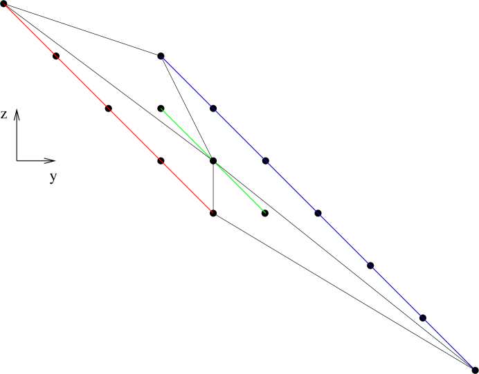
Figure 4: The dual cone $\sigma^{\vee}$ for $Y^{5,1}$. The $a$ type operators correspond to lattice points along the red line, the $b$ type operators to lattice points along the green line, and the $c$ type operators to lattice points along the blue line.

One can also see the $a$, $b$, and $c$ type operators emerge from the toric diagram for the cones over the $Y^{p,q}$. Recall [9] that the toric cone is given by the four vectors:

$$e_{1}=(1,0,0)\;;\;\;\;e_{2}=(1,1,0)\;;\;\;\;e_{3}=(1,p,p)\;;\;\;\;e_{4}=(1,p-q-1,p-q)\ .$$ (48)

The dual cone $\sigma^{\vee}$ must then be bounded by the vectors orthogonal to the faces of $\sigma$:

$$e_{1}^{\vee}=(0,0,-1)\;;\;\;\;e_{2}^{\vee}=(-p,p,-p+1)\;;\;\;\;e_{3}^{\vee}=(-p,-q,q+1)\;;\;\;\;e_{4}^{\vee}=(0,-p+q,p-q-1)\ .$$ (49)

We now study $\sigma^{\vee}$. Notice that $e_{1}^{\vee}$ and $e_{4}^{\vee}$ lie along the line $x=0$ and $z=-y-1$. This line will thus include $p-q+1$ lattice points, and we tentatively identify these points with the $a_{i}$. Similarly, $e_{2}^{\vee}$ and $e_{3}^{\vee}$ lie along the line $x=-p$ and $z=-y+1$. This line includes $p+q+1$ lattice points, and we identify these points with the $c_{i}$.

Finally, consider the three lattice points $(-1,0,0)$, $(-1,1,-1)$ and $(-1,-1,1)$. These three points would be good candidates for the $b_{i}$ – the points would lead to expected relations of the form $ac\sim b^{p}$. Note that $(-1,1,-1)$ lies on the plane spanned by $e_{1}^{\vee}$ and $e_{2}^{\vee}$:

$$(-1,1,-1)=\frac{1}{p}(e_{1}^{\vee}+e_{2}^{\vee})\ ,$$ (50)

and similarly

$$(-1,-1,1)=\frac{1}{p}(e_{3}^{\vee}+e_{4}^{\vee})\ .$$ (51)

Thus these three lattice points do indeed lie inside $\sigma^{\vee}$.

These three sets of lattice points $a_{i}$, $b_{i}$, and $c_{i}$ span the cone $\sigma^{\vee}$. More precisely, we expect that for any lattice point $p$ inside $\sigma^{\vee}$,

$$p=\sum\ell_{i}a_{i}+\sum m_{i}b_{i}+\sum n_{i}c_{i}$$ (52)

for $\ell_{i}$, $m_{i}$ and $n_{i}$ non-negative integers.

Appendix C From the Metric to the Chiral Ring

In this section, we will relate the $a_{i}$, $b_{j}$, and $c_{k}$ building blocks of the chiral ring directly to the metric coordinates on the Calabi-Yau cone. It turns out that it is just as easy to work out the relationship for all the $Y^{p,q}$ at once.

We choose coordinates on $Y^{p,q}$ such that the Sasaki-Einstein metric takes the form [10, 11]

$$ds^{2} = \frac{1-y}{6}\left(d\theta^{2}+\sin^{2}\theta d\phi^{2}\right)+\frac{1}{w(y)v(y)}dy^{2}$$ (53)

$$+ \frac{v(y)}{9}\left(d\psi-\cos\theta d\phi\right)^{2}+w(y)\left(d\alpha+f(y)(d\psi-\cos\theta d\phi)\right)^{2}$$

with the three functions $f(y),v(y),w(y)$ given by

$$w(y) = 2\frac{b-y^{2}}{1-y}$$ (54)

$$v(y) = \frac{b-3y^{2}+2y^{3}}{b-y^{2}}$$ (55)

$$f(y) = \frac{b-2y+y^{2}}{6(b-y^{2})}.$$ (56)

For the metric to be complete,

$$b=\frac{1}{2}-\frac{p^{2}-3q^{2}}{4p^{3}}\sqrt{4p^{2}-3q^{2}}\ .$$ (57)

The coordinate $y$ is allowed to range between the two smaller roots of the cubic $b-3y^{2}+2y^{3}$:

$$y_{1} = \frac{1}{4p}\left(2p-3q-\sqrt{4p^{2}-3q^{2}}\right)\ ,$$ (58)

$$y_{2} = \frac{1}{4p}\left(2p+3q-\sqrt{4p^{2}-3q^{2}}\right)\ .$$ (59)

The period of $\alpha$ is $2\pi\ell$ where

$$\ell=-\frac{q}{4p^{2}y_{1}y_{2}}\ .$$ (60)

The remaining coordinates are allowed the following ranges: $0\leq\theta<\pi$, $0\leq\phi<2\pi$, and $0\leq\psi<2\pi$.

In these coordinates the scalar Laplacian is

$$\nabla^{2} = \frac{6}{1-y}\frac{1}{\sin\theta}\frac{\partial}{\partial\theta}\sin\theta\frac{\partial}{\partial\theta}+\frac{6}{1-y}\frac{1}{\sin^{2}\theta}\frac{\partial^{2}}{\partial\phi^{2}}$$

$$+\left(\frac{9}{v}-\frac{6}{1-y}+\frac{6}{1-y}\frac{1}{\sin^{2}\theta}\right)\frac{\partial^{2}}{\partial\psi^{2}}+\frac{1}{1-y}\frac{\partial}{\partial y}vw(1-y)\frac{\partial}{\partial y}$$

$$+\left(\frac{9f^{2}}{v}+\frac{1}{w}\right)\frac{\partial^{2}}{\partial\alpha^{2}}+\frac{12}{1-y}\frac{\cos\theta}{\sin^{2}\theta}\frac{\partial^{2}}{\partial\phi\partial\psi}-\frac{18f}{v}\frac{\partial^{2}}{\partial\alpha\partial\psi}\ .$$

C.1 Chiral Primary Solutions

The Laplacian on the cone $dr^{2}+r^{2}ds^{2}$ over $Y^{p,q}$ can be written as

$$\Box=\frac{1}{r^{5}}\frac{\partial}{\partial r}r^{3}\frac{\partial}{\partial r}+\frac{1}{r^{2}}\nabla^{2}\ .$$ (62)

This cone is a Kaehler manifold and $\Box=2(\partial\partial^{\dagger}+\partial^{\dagger}\partial)$. Thus any holomorphic function should satisfy the Laplace equation, $\Box\omega=0$. These holomorphic functions are our chiral primary operators.

Martelli and Sparks [9] provide three meromorphic functions on the cone over $Y^{p,q}$:

$$z_{1} = e^{i\phi}\tan\frac{\theta}{2}$$ (63)

$$z_{2} = e^{-6i\alpha-i\psi}\frac{2}{\sin\theta}\prod_{i=1}^{3}(y-y_{i})^{-\frac{1}{2y_{i}}}$$ (64)

$$z_{3} = \frac{1}{2}r^{3}e^{i\psi}\sin\theta\prod_{i=1}^{3}(y-y_{i})^{1/2}\ .$$ (65)

One can check that away from their singularities, these $z_{i}$ satisfy $\Box z_{i}=0$. Of these three functions, $z_{3}$ is also holomorphic. The function $z_{1}$ has a singularity at $\theta=\pi$, while $z_{2}$ has singularities at $\theta=0$, $\theta=\pi$, and $y=y_{2}$. (Recall that $y_{1}<0$.) The function $z_{2}$ has the additional pathology of not being periodic under shifts $\alpha\to\alpha+2\pi\ell$.

Using these three $z_{i}$, we would like to assemble a family of better behaved holomorphic functions on the cone. For this family, we assume the ansatz

$$F_{mna}(z_{i}) = z_{1}^{m}z_{2}^{-a/6}z_{3}^{n-a/6}$$

$$= r^{3n-a/2}e^{im\phi}e^{in\psi}e^{ia\alpha}\sin^{n+m}\frac{\theta}{2}\cos^{n-m}\frac{\theta}{2}\prod_{i=1}^{3}(y-y_{i})^{e_{i}}$$

where

$$e_{i}=\frac{1}{12y_{i}}\left(a(1-y_{i})+6ny_{i}\right)\ .$$ (67)

To be free of singularities in $\theta$, we must take $-n\leq m\leq n$. To be free of singularities in $y$, we have the two conditions $e_{i}\geq 0$ for $i=1$, 2. We also have a number of periodicity constraints. For periodicity in $\alpha$, we need $a=P/\ell$ where $P$ is an integer. We will assume that $\phi$ is periodic under shifts by $2\pi$ and that $\phi+\psi$ is periodic under shifts by $4\pi$. These constraints then imply that $m$ and $n$ are either both integer or both half-integer.

One easy set of holomorphic functions can be found by setting $a=0$. We find

$$b_{1} = z_{3}z_{1}^{-1}=r^{3}e^{i(\psi-\phi)}\cos^{2}\frac{\theta}{2}\prod_{i=1}^{3}(y-y_{i})^{1/2}$$ (68)

$$b_{2} = z_{3}=r^{3}e^{i\psi}\sin\frac{\theta}{2}\cos\frac{\theta}{2}\prod_{i=1}^{3}(y-y_{i})^{1/2}$$ (69)

$$b_{3} = z_{3}z_{1}=r^{3}e^{i(\psi+\phi)}\sin^{2}\frac{\theta}{2}\prod_{i=1}^{3}(y-y_{i})^{1/2}$$ (70)

where we have identified these objects with the holomorphic monomials of the previous section. Superficially, $b_{1}$ seems not to be single valued at $\theta=0$ while $b_{3}$ would not be single valued at $\theta=\pi$. In fact, at these poles, the metric on $Y^{p,q}$ degenerates such that the good angular coordinate at $\theta=0$ is no longer $\psi$ but $\psi-\phi$ and at $\theta=\pi$, $\psi+\phi$.

To find the other holomorphic functions, we explore the boundaries of the singularity conditions on $y$. In particular, consider the limit $e_{i}=0$. In the case $i=1$, we find that

$$a=-\frac{6ny_{1}}{1-y_{1}}\;;\;\;\;e_{2}=\frac{np}{q+p}\ .$$ (71)

The periodicity condition on $\alpha$ implies that

$$n=\frac{q+p}{2}P\ .$$ (72)

Choosing the smallest nontrivial value $P=1$ that avoids a singularity at $y=y_{2}$, we find that $e_{2}=p/2$. These operators take the form

$$c_{i_{m}}=z_{1}^{m}r^{\Delta}e^{i(p+q)\psi/2+i\alpha/\ell}\left(\sin\frac{\theta}{2}\cos\frac{\theta}{2}\right)^{(p+q)/2}(y-y_{2})^{p/2}(y-y_{3})^{e_{3}}\ ,$$ (73)

where the R-charge

$$R=\frac{2}{3}\Delta=p\frac{2y_{2}}{y_{2}-y_{1}}\ ,$$ (74)

and

$$e_{3}=\frac{q+p}{4}\left(1-\frac{y_{1}(1-y_{3})}{y_{3}(1-y_{1})}\right)\ .$$ (75)

We have labelled these operators to suggest the relationship to the $c_{i}$ of the previous section. These operators fill out a $q+p+1$ dimensional representation of $SU(2)$.

Next consider the limit $e_{2}=0$, in which case

$$a=-\frac{6ny_{2}}{1-y_{2}}\;;\;\;\;e_{1}=\frac{np}{p-q}\ .$$ (76)

Periodicity on $\alpha$ now implies that

$$n=-\frac{p-q}{2}P\ .$$ (77)

Choosing the smallest nontrivial value of $P=-1$ that avoids a singularity, we find that $e_{1}=p/2$. These operators take the form

$$a_{i_{m}}=z_{1}^{m}r^{\Delta}e^{i(p-q)\psi/2-i\alpha/\ell}\left(\sin\frac{\theta}{2}\cos\frac{\theta}{2}\right)^{(p-q)/2}(y-y_{1})^{p/2}(y-y_{3})^{e_{3}}\ ,$$ (78)

where the R-charge

$$R=\frac{2}{3}\Delta=-p\frac{2y_{1}}{y_{2}-y_{1}}\ ,$$ (79)

and

$$e_{3}=\frac{p-q}{4}\left(1-\frac{y_{2}(1-y_{3})}{y_{3}(1-y_{2})}\right)\ .$$ (80)

These operators fill out a $p-q+1$ dimensional representation of $SU(2)$ like the $a_{i}$ of the previous section.

Using for example the table in [13], one may easily check that the R-charges computed from these holomorphic functions agrees with the R-charges computed from field theory. In other words, (79) agrees with (46) and (74) is eqal to (47).

We now check that these $a_{j}$ and $c_{j}$ are indeed single valued at $y=y_{2}$ and $y=y_{1}$ respectively. From the metric, we see that at $y=y_{i}$, the good angular coordinate is no longer $\alpha$ but

$$\alpha+f(y_{i})\psi=\alpha+\frac{1}{6}\frac{y_{i}-1}{y_{i}}\psi\ .$$ (81)

Correspondingly, the exponent for the $a_{j}$ can be written

$$\frac{p-q}{2}\psi-\frac{1}{\ell}\alpha=-\frac{1}{\ell}\left(\alpha+\frac{(q-p)\ell}{2}\psi\right)$$ (82)

and it is not difficult to check that

$$\frac{(q-p)\ell}{2}=\frac{y_{2}-1}{6y_{2}}\ .$$ (83)

For the $c_{j}$, we find that

$$\frac{p+q}{2}\psi+\frac{1}{\ell}\alpha=\frac{1}{\ell}\left(\alpha+\frac{(p+q)\ell}{2}\psi\right)$$ (84)

and

$$\frac{(p+q)\ell}{2}=\frac{y_{1}-1}{6y_{1}}\ .$$ (85)

References

- [1] I. R. Klebanov and M. J. Strassler, “Supergravity and a confining gauge theory: Duality cascades and chiSB-resolution of naked singularities,” JHEP 0008, 052 (2000) [arXiv:hep-th/0007191].
- [2] R. Gopakumar and C. Vafa, “On the gauge theory/geometry correspondence,” Adv. Theor. Math. Phys. 3, 1415 (1999) [arXiv:hep-th/9811131].
- [3] S. Kachru, R. Kallosh, A. Linde and S. P. Trivedi, “De Sitter vacua in string theory,” Phys. Rev. D 68, 046005 (2003) [arXiv:hep-th/0301240].
- [4] I. R. Klebanov and E. Witten, “Superconformal field theory on threebranes at a Calabi-Yau singularity,” Nucl. Phys. B 536, 199 (1998) [arXiv:hep-th/9807080].
- [5] D. R. Morrison and M. R. Plesser, “Non-spherical horizons. I,” Adv. Theor. Math. Phys. 3, 1 (1999) [arXiv:hep-th/9810201].
- [6] A. Kehagias, “New type IIB vacua and their F-theory interpretation,” Phys. Lett. B 435, 337 (1998) [arXiv:hep-th/9805131].
- [7] K. Altmann, “The versal Deformation of an isolated toric Gorenstein Singularity,” arXiv:alg-geom/9403004.
- [8] B. Feng, A. Hanany and Y. H. He, “D-brane gauge theories from toric singularities and toric duality,” Nucl. Phys. B 595, 165 (2001) [arXiv:hep-th/0003085].
- [9] D. Martelli and J. Sparks, “Toric geometry, Sasaki-Einstein manifolds and a new infinite class of AdS/CFT duals,” arXiv:hep-th/0411238.
- [10] J. P. Gauntlett, D. Martelli, J. Sparks and D. Waldram, “Supersymmetric AdS(5) solutions of M-theory,” Class. Quant. Grav. 21, 4335 (2004) [arXiv:hep-th/0402153].
- [11] J. P. Gauntlett, D. Martelli, J. Sparks and D. Waldram, “Sasaki-Einstein metrics on S(2) x S(3),” arXiv:hep-th/0403002.
- [12] M. Bertolini, F. Bigazzi and A. L. Cotrone, “New checks and subtleties for AdS/CFT and a-maximization,” arXiv:hep-th/0411249.
- [13] S. Benvenuti, S. Franco, A. Hanany, D. Martelli and J. Sparks, “An infinite family of superconformal quiver gauge theories with Sasaki-Einstein duals,” arXiv:hep-th/0411264.
- [14] S. Franco, A. Hanany, Y. H. He and P. Kazakopoulos, “Duality walls, duality trees and fractional branes,” arXiv:hep-th/0306092.
-
[15]
S. Franco, Y. H. He, C. Herzog and J. Walcher,
“Chaotic duality in string theory,”
Phys. Rev. D 70, 046006 (2004)
[arXiv:hep-th/0402120];
“Chaotic Cascades for D-branes on Singularities,” proceedings of the Cargese Summer School 2004, [arXiv:hep-th/0412207]. - [16] C. P. Herzog, Q. J. Ejaz and I. R. Klebanov, “Cascading RG flows from new Sasaki-Einstein manifolds,” arXiv:hep-th/0412193.
- [17] I. R. Klebanov and A. A. Tseytlin, “Gravity duals of supersymmetric SU(N) x SU(N+M) gauge theories,” Nucl. Phys. B 578, 123 (2000) [arXiv:hep-th/0002159].
- [18] K. Konishi, “Anomalous Supersymmetry Transformation Of Some Composite Operators In Sqcd,” Phys. Lett. B 135, 439 (1984).
- [19] A. Butti, M. Grana, R. Minasian, M. Petrini and A. Zaffaroni, “The Baryonic Branch of Klebanov-Strassler Solution: a Supersymmetric Family of SU(3) Structure Backgrounds,” arXiv:hep-th/0412187.
- [20] M. Grana, R. Minasian, M. Petrini and A. Tomasiello, “Supersymmetric backgrounds from generalized Calabi-Yau manifolds,” JHEP 0408, 046 (2004) [arXiv:hep-th/0406137].
-
[21]
S. S. Gubser, C. P. Herzog and I. R. Klebanov,
“Symmetry breaking and axionic strings in the warped deformed conifold,”
JHEP 0409, 036 (2004)
[arXiv:hep-th/0405282];
“Variations on the warped deformed conifold,” arXiv:hep-th/0409186. - [22] D. Berenstein, “Reverse geometric engineering of singularities,” JHEP 0204, 052 (2002) [arXiv:hep-th/0201093].
- [23] K. Intriligator and B. Wecht, “The exact superconformal R-symmetry maximizes a,” Nucl. Phys. B 667, 183 (2003) [arXiv:hep-th/0304128].
- [24] D. Kutasov, A. Parnachev and D. A. Sahakyan, “Central charges and U(1)R symmetries in N = 1 super Yang-Mills,” JHEP 0311, 013 (2003) [arXiv:hep-th/0308071].
- [25] N. Seiberg, “Electric - magnetic duality in supersymmetric nonAbelian gauge theories,” Nucl. Phys. B 435, 129 (1995) [arXiv:hep-th/9411149].
-
[26]
D. Amati, K. Konishi, Y. Meurice, G. C. Rossi and G. Veneziano,
“Nonperturbative Aspects In Supersymmetric Gauge Theories,”
Phys. Rept. 162, 169 (1988);
K. A. Intriligator and N. Seiberg, “Lectures on supersymmetric gauge theories and electric-magnetic duality,” Nucl. Phys. Proc. Suppl. 45BC, 1 (1996) [arXiv:hep-th/9509066];
M. A. Shifman, “Nonperturbative dynamics in supersymmetric gauge theories,” Prog. Part. Nucl. Phys. 39, 1 (1997) [arXiv:hep-th/9704114]. -
[27]