hep-th/0504230
ULB-TH 05-08
The structure of at higher levels – a first algorithmic approach
Thomas Fischbacher
Physique Théorique et Mathématique and
International Solvay Institutes, Université Libre de Bruxelles,
Campus Plaine C.P. 231, B–1050 Bruxelles, Belgium
tf@cip.physik.uni-muenchen.de
Abstract
The conjecture of a hidden symmetry of M-theory is supported by the close connection between the dynamics of supergravity near a spacelike singularity and a truncation of an one-dimensional -model with symmetry where all representations beyond level are omitted. If this conjecture is right, higher-level representations should especially capture the dynamics of further M-theory degrees of freedom. Unfortunately, the level by level determination of commutators which is necessary to extend the model to higher levels is both an involved and toilsome task that requires computer aid. In this work, some of the relevant problems are exposed and algorithmic methods are developed which simplify key steps in the determination of explicit commutators at higher levels. As an application, we compute the commutator of the level-two six-form with itself.
1 Introduction
Since Witten’s discovery [17] that the strong coupling limit of the five consistent ten dimensional superstring theories may be an eleven-dimensional theory whose low energy regime is the unique known eleven-dimensional supergravity, there has been a lot of activity trying to get a better understanding of the nature of this strong coupling regime of string theory, as this is is a highly promising candidate for the complete unified description of the dynamics of all the fundamental forces. While a lot could be derived about this theory in the last decade, our picture is still quite incomplete, and this is mirrored by the preliminary incomplete name M-theory.
As the study of symmetries – possibly hidden and showing up only in certain limits of a model – has been extremely fruitful for the advancement of our understanding of fundamental physics, during the last century, often leading to a major breakthrough, any indication of a not yet well understood symmetry of M-theory should be considered as a potential important clue, and subjected to close investigation. While the existence of hidden exceptional symmetries of eleven-dimensional supergravity, especially the hidden global symmetry that occurs in Kaluza-Klein reduction on a -dimensional torus, is well known (see e.g. [3] for an introduction), and speculations about a hidden global infinite-dimensional Kac-Moody symmetry also have been around for a long time [12], the conjecture of a fundamental symmetry of M-theory recently gained interest by the discovery that for the bosonic sector of eleven-dimensional supergravity in a setting close to a spacelike ‘big bang’ singularity (where spatially separated points become causally disconnected), the degrees of freedom of the metric show chaotic oscillations of BKL type [2] that can be described by relativistic billiards [5, 4, 6] taking place in a region of the shape of the fundamental Weyl chamber of . Intriguingly, a one-dimensional -model [7] constructed from a truncation of to the first three levels of a decomposition [16] is able to capture and reproduce the dynamics of a correspondingly truncated expansion in terms of gradients of supergravity in the previously described limit. While this already is a highly nontrivial result, one may still be sceptical whether this correspondence may be extended to higher levels. At least, seems to contain all the fields necessary to represent higher gradients of the -form and -form potential as well as the ‘dual’ graviton. Besides those, there are many other representations that are conjectured to be linked to other dynamical (potentially even yet unknown) degrees of freedom of M-theory. First promising indications that such a description of M-theory via an -model may indeed work are given by the highly nontrivial observation that it may be reconciled (in a truncation to low levels) with both (massive) and supergravity [13, 14], as well as the possible correspondence of singlets at quite high levels to , ,…corrections of M-theory [9].
Clearly, it is essential to perform an extension of the construction beyond level three. As we will see, this is bound to require some quite involved algorithms, and hence this line of research may well benefit from scientific exchange with computer scientists specialized in symbolic algebra. Therefore, the present article is somewhat more verbose than one targeted exclusively at a string theory audience. While it is not expected of readers with a specialization in symbolic algebra to comprehend all of the physics upon first reading, at least the relation between the relevant concepts should become clear. While we will be concerned exclusively with the determination of commutators for the Borel subalgebra of in this work, details on the construction of the model up to level three can be found in [8].
2 Conventions
In the following, we will make extensive use of irreducible representations of the Lie algebra that are obtained by applying mixed-symmetry Young projectors on tensor powers of the fundamental vector representation. We use the usual convention of first symmetrizing over rows, then symmetrizing over columns of a Young tableau, i.e.
| (1) |
It is furthermore convenient to lay out all the indices of a tensor carrying a single irreducible representation in a form that directly mirrors the shape of the corresponding symmetrizer’s tableau. However, as we will mostly have to deal with short symmetrizations and long anti-symmetrizations in the analysis of , we will rotate our tableaux by a counterclockwise quarter-turn. Thus, from now on, we write e.g.
| (2) |
for the ‘dual graviton’ generator at level three in the decomposition of . Despite this notation, which is rotated solely for obvious typographic reasons, we will still speak of the symmetrization of rows and anti-symmetrization of columns!
We will also extensively apply symmetrization and anti-symmetrization operations to groups of indices. While this is usually denoted with brackets or parentheses around groups of indices, such as in111As usual, we define anti-symmetrizers as projectors, e.g. .
| (3) |
this ad-hoc notation has two important drawbacks:
-
•
It is highly unpractical for more complicated situations with interlocking symmetrizations.
-
•
Positional information is used to convey information about symmetrizations.
In particular, there is no reasonable way to translate an expression like
| (4) |
to full bracketed-indices symmetrization notation. Such quantities are, however, bound to appear in the analysis of higher levels of hyperbolic Kac-Moody symmetries.
The second problem mentioned has an important conceptual aspect: there are two different ways to apply an (anti-)symmetrization to a given mixed-symmetry tensor. One has to discern between using the antisymmetry in indices of the same column to exchange boxes, i.e.
| (5) |
and applying a symmetrization to index names, as in:
| (6) |
which would correspond to ‘placing brackets around ’.
One can make the idea rigorous that the first operation acts on the right, while the second one acts on the left of the operation of naming tensor indices, hence we will denote the first kind of symmetrization as a box shifting symmetrization, and the second one as an index relabeling symmetrization. Note that box shifting symmetrizations are conceptually tied to individual columns of a single (mixed-symmetry) tensor, while index relabeling symmetries are more naturally associated to entire sums, not individual summands, as they amount to introducing an extra factor. A large part of the algebraic complexity of the higher levels is related to the fundamental difference between these two concepts.
We clearly need a new notation for index relabeling symmetrizations that overcomes the forementioned problems. We will use the convention to denote symmetrization in indices by appending a formal (pseudo-)factor to the right of the term, and likewise anti-symmetrization in these indices by a formal factor . This definition implicitly contains the rule to apply such factors one by one from the left to the right to a term, replacing by , where are fresh indices, and substituting free indices , , etc. in all factors to the left of it. If it helps to make a point, we will occasionally include trivial one-index symmetrization factors like in our formulae.
To give an example, applying a specific Young projector may now be written as:
| (7) |
The numerical factor , in our example, that makes a sequence of a tableau symmetrization followed by a tableau anti-symmetrization an idempotent projector, is given by
| (8) |
(For every box in the tableau, there is exactly one hook, which consists of this box and all that lie either in the same row and to the right of it, or in the same column and further down.)
Note that with this notation, it is very easy to make proper use of both box shifting and index relabeling symmetries. For example, we have:
| (9) |
This raises the question how to define normal forms for such expressions. This is an involved issue that has many technical and algorithmic aspects and hence is discussed in detail in the appendix in section A.1.2. In brief, the idea behind the scheme used in this work is to treat all extra (non-overlapping) index symmetrizations on a tensor as being ordered lexicographically, then using them one after another to put as many lexically small tensor indices into columns to the far right as possible. This means in particular (as is shown with an example in the appendix) that submitting a mixed-symmetry tensor in normal form to its associated Young symmetrization will in general produce a sum of more than one tensor in normal form. This is mostly due to our ignorance of more complicated relations between mixed symmetry representations with permuted indices, which are most easily expressed in terms of Garnir symmetries [11] – these will be explained in some more detail at the end of section 3.4.
Defining a normal form that takes into account all three types of column antisymmetrization, index relabeling, and Garnir symmetries, and can be computed with sufficient efficiency for an application to is not as inextricable as it may seem at first, but will not be discussed here, even if using such a normal form that differs from the one used here will eventually turn out to be inevitable when going to high levels. Note that if one would not have to deal with index relabeling symmetries, it would be possible to define normal forms of filled tableaux just such that in a tensor in normal form, all indices appear in lexically ascending order in every column as well as in every row. Any tensor can be transformed into a linear combination of tensors of that form by repeated application of Garnir as well as column antisymmetries. It is easy to see that this prescription has to be refined further to get unique normal forms in the presence of index relabeling symmetries, as is demonstrated by the following example:
| (10) |
One can imagine that the situation will get far more involved in situations where e.g. index relabeling symmetries touch indices that are not located at the boundary of the tableau.
A further issue concerns the use of epsilon tensors: in Young tableau index notation, an element of the algebra which appears in the -fold iterated commutator will carry indices. Typically, some of those will form columns of maximal length (here ) that could be extracted as extra factors . For the sake of a homogeneous presentation, we will not do so, and instead keep all columns of maximal length explicit.
3 The Borel subalgebra from the perspective
We start this section by reviewing a few ideas and facts from Cartan-Dynkin theory and its application to . The roots of the algebra lie on the unique even unimodular Lorentzian lattice . Taking the ten-dimensional scalar product to be
| (11) |
this lattice is spawned by these ten vectors of squared length two (cf. [1])
| (12) |
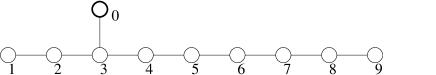
The Dynkin diagram encoding the geometrical structure of this lattice is given in figure 1.
3.1 Kac-Moody Algebras from Cartan matrices
One key property of Lie algebras is the geometry of their root lattice. Choosing a hyperplane through the origin that does not contain any further lattice point in order to separate lattice vectors into a ‘positive’ and ‘negative’ half and denoting positive lattice vectors that cannot be written as the sum of other positive lattice vectors as simple roots, this information can be concisely encoded in the Cartan matrix , which contains the scaled (not necessarily euclidean) scalar products of the simple roots:
| (13) |
The off-diagonal entries of a Cartan matrix are nonpositive integers, due to the indecomposability of the simple roots. Vice versa, it is possible to construct the Lie algebra from a generalized Cartan matrix: one first defines the Chevalley generators , with commutators satisfying
| (14) |
The algebra is then obtained first forming the free Lie algebra, which is spawned by all the commutators that can be built recursively from these generators, modulo the Jacobi identity
| (15) |
This free Lie algebra then has to be divided by the Serre relations:
| (16) |
For finite-dimensional Lie algebras, all roots have squared length . In the hyperbolic case – where we will take as our primary example – the metric on the root space is indefinite, and while there is just one generator associated to every root with (as in the finite-dimensional case), the multiplicity of roots inside the ‘light cone’, with , increases quite dramatically with increasing . While the Jacobi and Serre relations determine the structure of the Lie algebra, it is a difficult and basically still unsolved problem to effectively identify those multiple commutators of Chevalley generators that vanish due to the Serre relations, which may be revealed only after multiple applications of the Jacobi identity.
While one may construct a Lie algebra basis as well as determine the structure constants directly from the simple roots, it is frequently more convenient and more useful to identify a simple subalgebra that has a simple geometrical description by omitting one (or more than one) simple root, and slice the algebra into irreducible representations of this sub-algebra, graded by the number of occurrences of the operator or corresponding to the omitted root . This leads to the presentation of commutators in the language of tensors of the sub-algebra. An example of this technique, the decomposition of in terms of its sub-algebra, can be found in appendix B of [15].
In this work, we limit our analysis to Borel subalgebra commutation relations that are schematically of the form
| (17) |
Most of the technical complication comes from the demand to work not with explicit roots, but abstract tensor equations, and the combinatorical infeasibility to use naive (anti-)symmetrization by generating all permutations if more than eight indices have to be (anti)-symmetrized. Hence, the question arises how to organize calculations in such a way that maximal use can be made of overlaps with pre-existing symmetries.
3.2 The decomposition of at level
The determination of commutators for the algebra not only gets more and more voluminous with increasing level, one also has to use an increasing number of different algebraic tricks with increasing level. Also, some steps performed for the first few levels of the construction can be interpreted in multiple – sometimes unexpected – ways, and often, only one interpretation can be suitably generalized to be of use for higher levels as well.
Hence, it makes sense to start the discussion of higher levels with a brief review of the derivation of commutators up to level , where we mark those steps in the construction that require closer inspection, resp. modification, when going to higher levels with . A more detailed discussion of the nature of these steps will then be given in section 3.4.
One important tool in the derivation of commutation relations is the representation table in [16], whose first few entries we quote for convenience:
| dim | ||||||
| ( 0 0 1 0 0 0 0 0 0) | 0 0 0 0 0 0 0 0 0 | 2 | 120 | 1 | 1 | |
| ( 0 0 0 0 0 1 0 0 0) | 1 2 3 2 1 0 0 0 0 | 2 | 210 | 1 | 1 | |
| ( 1 0 0 0 0 0 0 1 0) | 1 3 5 4 3 2 1 0 0 | 2 | 440 | 1 | 1 | |
| ( 0 0 0 0 0 0 0 0 1) | 2 4 6 5 4 3 2 1 0 | 0 | 10 | 8 | 0 | |
| ( 0 0 1 0 0 0 0 0 1) | 2 4 6 5 4 3 2 1 0 | 2 | 1155 | 1 | 1 | |
| ( 2 0 0 0 0 0 0 0 0) | 1 4 7 6 5 4 3 2 1 | 2 | 55 | 1 | 1 | |
| ( 0 1 0 0 0 0 0 0 0) | 2 4 7 6 5 4 3 2 1 | 0 | 45 | 8 | 0 | |
| ( 0 0 0 0 0 1 0 0 1) | 3 6 9 7 5 3 2 1 0 | 2 | 1848 | 1 | 1 | |
| ( 1 0 0 1 0 0 0 0 0) | 2 5 8 6 5 4 3 2 1 | 2 | 1848 | 1 | 1 | |
| ( 0 0 0 0 1 0 0 0 0) | 3 6 9 7 5 4 3 2 1 | 0 | 252 | 8 | 0 | |
| ( 1 0 0 0 0 0 0 1 1) | 3 7 11 9 7 5 3 1 0 | 2 | 3200 | 1 | 1 | |
| ( 0 0 0 0 0 0 0 0 2) | 4 8 12 10 8 6 4 2 0 | 0 | 55 | 8 | 0 | |
| ( 0 1 0 0 0 1 0 0 0) | 3 6 10 8 6 4 3 2 1 | 2 | 8250 | 1 | 1 | |
| ( 1 0 0 0 0 0 1 0 0) | 3 7 11 9 7 5 3 2 1 | 0 | 1155 | 8 | 1 | |
| ( 0 0 0 0 0 0 0 1 0) | 4 8 12 10 8 6 4 2 1 | -2 | 45 | 44 | 1 |
At level one, there is the single three-form corresponding to the root . As there is only a single six-form at level two, the only sensible level two commutator that can be written down is
| (18) |
As the normalization of can be chosen arbitrarily, we set the coefficient .
The level three, we get a single tensor of mixed symmetry. Again, the most general ansatz for the level three commutator is
| (19) |
as there are only two different ways how to distribute indices from two columns of lengths (6,3) to two columns of lengths (8,1). If we make use of the identity
| (20) |
and the freedom in the normalization of , this can be reduced to
| (21) |
In order to obtain an expression for without the extra index relabeling symmetrizations in terms of commutators , we first apply an index relabeling symmetrization enforcing the column anti-symmetry of : to the entire expression:
| (22) |
From this point on, we will only work with terms with the proper column symmetry .
Besides the desired term, we get an extra contribution where the tableau structure does not match the index symmetrizations. This can be eliminated by making use of the Jacobi identity in the form
| (23) |
which can be reduced to an equation between tensors by use of the definitions (21,32)
| (24) |
which then has to be brought to symmetry:
| (25) |
This can then be used to reduce (LABEL:e3def-resymmetrized) to
| (26) |
which is of the desired form.
3.3 at level
When going to level , a few new features are encountered. First and foremost, the commutator will now contain two different representations. The most general ansatz which corresponds to (19) for level now is
| (27) |
taking into account all possible ways to re-distribute indices from the three columns to two columns of length , resp. three columns of length . Clearly, we have , due to the anti-symmetry in . This approach, however, does not yet fully appreciate the mixed symmetry of the tensors on the right hand side. Thinking of as a linear combination of basis tensors that diagonalize the regular part of the corresponding Young projector, we can use the fact that sequential application of any mixed-symmetry projection (i.e. any arbitrary distribution of the indices to symmetrize and anti-symmetrize over) corresponding to a tensor of this particular form to any such tensor, potentially with a different index distribution, followed by Young projections to the symmetries of the tensors on the left hand side, yields either zero or (up to an integer multiple that can be absorbed in the normalization) just one specific combination:
| (28) |
Likewise for the symmetric rank-2 contribution:
| (29) |
Hence, if we start with
| (30) |
we may in principle be able to derive the form of the commutator by making use of the Jacobi identity in the schematic form . Before we discuss this somewhat subtle issue further, we give the result. The only relevant nonvanishing commutator is:
| (31) |
3.4 On the role of the Jacobi identity
As the structure of the Lie algebra is determined fully by the Serre relations and the Jacobi identity, and both enter (indirectly) into the determination of root multiplicities via the Peterson formula, one may ask the question whether the problem that the Serre relations and Jacobi identity are interlocked in an unwieldy way may be circumnavigated by trying to trade the Serre relations for the known root multiplicities in the level by level determination of the structure constants. In other words, taking a commutator definition of the form of (30), what information can be extracted from the Jacobi identity at the given level? In particular, is it possible to derive further relations of the form (25) that can be used to simplify the commutator?
A head-on approach to this problem at level is to systematically generate all possible commutator structures of tensors and all linear relations between three of them determined by the Jacobi identity. Taking all possible index distributions into account, and re-symmetrizing to a given desired Young tableau column antisymmetry, this is bound to produce all the relevant relations that can be obtained in such a way. Clearly, this procedure soon becomes infeasible even on a powerful computer due to combinatorical explosion, but it is nevertheless important to try this for the following reasons: First of all, there are many opportunities where even a small mistake in the implementation of an extensive algebraic algorithm can lead to wrong results that are hard to detect with the naked eye, do not occur for many simple test cases, but lead to inconsistencies in large calculations. An extensive analysis like the one described is one of the few but crucially important ‘smoke tests’ available that help to discover program bugs. Unfortunately, it also can only give binary information: either simplification of a considerable number of linear equations (typically equations containing in total summands with twelve-index tensors at level four) gives nonsensical relations like a vanishing commutator that is known to be nonzero, or a set of equations that seem to make sense. In the former case, the so far only way to find a bug seems to be to print out a detailed trace of all term transformations in the program and check this manually – which easily becomes highly frustrating sysiphus labour in the long run. The second reason is that this is the conceptually simplest approach to the systematic determination of commutators of the form for . While one might initially try to start with a definition for and use the Jacobi identity to derive the commutator by splitting to a term of the schematic form , and then continue with this procedure to successively determine , etc., this approach is complicated considerably by the fact that a direct application requires using a definition of the schematic form , while one starts with an equation of the form , with tensors belonging to a variety of irreducible representations on the right hand side, that first has to be solved. Developing the relevant algorithmic techniques to efficiently automatize this is simplified greatly by knowing the right answer from the start from a conceptually simpler and hence more robust approach that may well be not efficient enough to be used for high levels.
Efficient algorithms to generate a complete set of level double-commutator identities from the Jacobi identity are described in appendices A.2,A.3. These furthermore have to be instantiated with all possible distributions of the indices to the fundamental tensors, modulo permutation of groups of three indices, e.g. , and then re-symmetrized in all possible different ways to the desired symmetry. Special care has to be taken with substitutions of commutator definitions: it is easy to overlook that an equation of the form may only be substituted into a term containing after suitable index re-labeling if the distribution of indices in the (anti-)symmetrizers relative to the distribution of those indices to the columns of can be made to agree. Efficiently finding suitable index relabelings so that a substitution can be applied is a further nontrivial task.
Looking at the step from level to , the major points that are not yet visible at level and require generalization for an algorithmic approach are the following:
: For a simplified uniform systematic algorithmic treatment, all commutator definitions have to be given in a form such that both left hand side and right hand side make the column anti-symmetries of the tensors in the commutator explicit. Hence, even the commutator should be given in the form
| (32) |
whose anti-symmetrization redundancy might look slightly nonsensical, but actually helps greatly to simplify many algorithms.
: One should use a sequence of Young tableau projections instead of just the corresponding column anti-symmetrizations to reduce commutator definitions.
: At least at level , trying to use the Jacobi identity to derive further relations between ‘wrongly symmetrized’ tensors of mixed symmetry seems to be a red herring. The Jacobi identity does not produce any new relations of the strict form . Even at level , it is perhaps more helpful to think of the corresponding identity as a consequence of a Garnir symmetry and not the Jacobi identity: for every pair of horizontally adjacent boxes in a tableau, there is a linear relation between all tableaus with fillings that can be obtained by permuting the indices in those two boxes, plus all below the left one, plus all above the right one, in all possible ways. The coefficients in that linear relation are , and determined by the constraint that the relative sign between terms that differ by an exchange of adjacent boxes is . Thus, for the two horizontally adjacent boxes in the tensor , we get the relation:
| (33) |
Anti-symmetrizing with then gives (25). Hence, if the notion of a tensor normal form already respected Garnir symmetries, the reduction from (LABEL:e3def-resymmetrized) to (26) would be automatic.
3.5 Beyond level four
There are a few obvious issues that have to be kept in mind when going from level four to level five. First of all, one no longer has one single commutator of the form , but two different level four representations whose commutators with have to be taken. Furthermore, one no longer can just normalize tensors such that they appear with coefficient in such a defining equation. The reason is that the representation at may a priori appear in the commutator of both representations with . One might still argue that it will presumably at least appear in the commutator of the representation with , as this commutator cannot produce the only other representation. If it were zero, the generators belonging to would have to commute not only with , but (via the Jacobi identity) also with , and (inductively) with all generators at higher level. Hence, the coefficient could be set to one in this particular commutator. Such reasoning cannot be carried any further, however, as the representation at level is in the tensor product of both representations with the level-one representation, which both carry further tensors. At level , we encounter outer multiplicities for the first time.
4 Conclusion
Lacking a powerful theory of the structure of hyperbolic Kac-Moody algebras, their possible relevance in gravitational physics – especially the conjectured role of for -theory – probably justifies going to great lengths to obtain detailed information about even only the first few elements of a finite truncation. This is virtually impossible to achieve to satisfactory depth via manual calculation, both due to the sheer number of steps and due to the inherent ineptness of humans to execute them in such large numbers without making mistakes. Hence, this task is bound to require computer aid. Unfortunately, the algorithmic side of this problem turns out as being of unusually high complexity, hence despite considerable technical effort, only very little could be achieved in this work in terms of new data about structure constants. The most important obstacle to further progress seems to be the unavailability of powerful tests that simplify the discovery and analysis of flaws and errors in algorithms and their implementations: while it is essential to try out various approaches to individual sub-problems (and, as it turns out, frequently change them when they have to be embedded into a larger context), all that can be done to validate an algorithm (not to speak of verification) is to use it to automatically generate all conceivable relations from a certain not too small set, semi-automatically check for inconsistencies, and – should they arise – eventually redo dozens of lengthy calculations by hand that involve tensors with more than ten indices, where one has to especially take great care about signs from index re-orderings. One has to note that certain problems are specific to situations with quite many indices, so that simple test cases frequently just do not exist. The problem may well be that even the appropriate questions have not yet been found that have to be asked, and answered, to make the validation phase more bearable. Addressing this problem presumably should be the most reasonable next step before changing the definition of normal forms such that Garnir symmetries are properly taken care of. Then, the issue of a systematic determination of commutators has to be addressed before the sigma-model can be extended to higher levels. As it turned out that the task of actually implementing the relevant algorithms is highly prone to sign and similar errors, and as debugging is complicated by the fact that it is virtually impossible to develop an intuition for such terms, a reference implementation in LISP that also can be used to redo the calculations presented here within reasonable calculation time will be made publicly available in the next release of [10].
Acknowledgments
The analysis presented here could not have been performed without helpful and encouraging discussions with Sophie de Buyl, Francois Englert, Marc Henneaux, and Laurent Houart from ULB, and Hermann Nicolai, and Kasper Peeters, and especially Axel Kleinschmidt from AEI. The author furthermore acknowledges financial support by the German Academic Exchange Service via the DAAD postdoc research program. This work was partially supported by IISN - Belgium (convention 4.4505.86), by the “Interuniversity Attraction Poles Programme – Belgian Science Policy” and by the European Commission FP6 programme MRTN-CT-2004-005104, in which the author is associated to V.U. Brussel.
Appendix A Algorithms
In this appendix we list algorithms that are used to address various parts of the problem.
A.1 Efficient index (anti-)symmetrization for tensors of high rank
The naive translation of the symmetrization/anti-symmetrization prescriptions for Young tableau projections to a computer algorithm reaches its limits quite early, often already with problems that – using some thought – easily can be done by hand. The primary underlying reason is that a naive execution of a task like e.g. the anti-symmetrization over nine indices generates different individual copies of a term with indices re-distributed in all possible ways which then usually have to be classified and subjected to further reductions. Nevertheless, quite many research problems where such manipulations are necessary are of such a structure that, given an unlimited amount of time and energy, the analysis could be taken to almost arbitrary depth. Not seldom, there is a considerable gap between the point where one can claim to have obtained a sufficiently deep understanding of the mathematical structure that going any further is not expected to produce valuable additional insights and the point where it becomes unfeasible to do calculations by hand.
This raises the question how to formalize those ideas that make the simple cases feasible by hand in such a way that they can be executed as effectively by a machine, only much faster and much more reliable than by a human. The key idea here is to make as much use of overlapping symmetrizers and anti-symmetrizers as possible.
A.1.1 Data Structures
While one may want to consider terms formed out of general products of tensors with mixed symmetry, we limit our discussion to the framework of Lie algebras, where the only product of terms is the commutator. Conceptually, this is also the most interesting case, as the issue of normal forms of terms will be more involved here than with simple tensor products. Additionally, we restrict ourselves to tensors with contravariant indices belonging to one algebra only. This last restriction will eventually have to be softened, at the very least to allow indices to be either all contravariant or all covariant, in order to represent commutators of the type. The case of more general base algebras than may also be studied, but the price that has to be paid is that the relation between irreducible representations and corresponding tableaux gets much more involved, hence this is not considered here.
Tensors
The most natural way to represent a tensor is as a tuple , where is the type of the tensor, is some abstract weight that will be used to normalize commutators, the shape of the Young tableau, and a vector of indices. On the pragmatic level, will also include information about a printable tensor name. We furthermore assume a strict order as well as addition to be defined on tensor weights, which will be used for sorting tensors, e.g. to determine normal forms for sums. The tableau shape must provide information about where to place an index from the linearized presentation in the tableau. This can be achieved e.g. by just recording the lengths of the rows of the tableau, and using the convention to record indices in normal reading order. Furthermore, must provide information that allows one to quickly extract all the indices belonging to a given column from . When building terms from tensors, it is useful not to put the tensor into the term as it is, but rather a tuple , where the tensor is supplemented by an extra bit of information describing whether reduction to normal form has been applied to this quantity or not. Note that data representations in a real implementations may not strictly adhere to these lines, as there might be practical reasons to e.g. include normalization information directly in the tensor data structure.
Terms
From tensors, we can recursively form sums and commutators. This is formalized by the definition of a term as a tuple , where is a (sorted) vector of summands with either a tensor or a commutator, and a coefficient. We impose the restriction that all summands must be of the same weight. The weight of a commutator is just the sum of the weights of its summands, and the weight of a term is just the weight of any of its summands. describes all the non-overlapping symmetrizations or anti-symmetrizations applied to the indices occurring inside this term. As index-symmetrization is an operation that is performed by multiplying a tensor onto an expression, this is most naturally represented on the level of terms, not individual tensors. In particular, symmetrizations will frequently stretch over indices belonging to two different sides of a commutator. is a list of pairs of a type bit discerning symmetrization from anti-symmetrization and a lexicographically ordered vector of index names. itself is ordered lexicographically with respect to the index name vectors.
As we may occasionally have to deal with the problem to extract a sign factor from a term, e.g. when bringing a commutator to normal form, which would have to be propagated through the ‘outer context’ of a subterm that is embedded in a term for normalization purposes, it can be convenient to be able to define normal form modulo a constant factor, hence we consider augmented terms which are tuples of a term with coefficient of the leading summand being , an overall factor , and a bit denoting whether and all its summands are guaranteed to be in normal form.
Commutators
A commutator is just a pair of a left and a right side, which both are augmented terms . Again, we augment this structure by an additional bit, , that provides information whether both the left and right entry are guaranteed to be in normal form, and furthermore whether the left side is smaller than the right side with respect to the order on terms, to be described next.
A.1.2 Normal Forms
Consequent use of augmented tensors, commutators, and terms allows to do many symbolic manipulations without unnecessary normalization steps for subterms that already are in normal form. Just as the definitions of commutators and terms have to recursively refer to one another, so do the definitions of their respective normal forms. We define a term to be in normal form, if its summands are in normal form and sorted in ascending order with respect to the order that treats a commutator as smaller than any tensor, compares commutators lexicographically, and orders tensors first by their type , then by their index distribution (which is assumed to be normalized), and read for the purpose of ordering in Kanji reading order (column by column right to left, every column up to down). A commutator is in normal form if the summands of the left side are smaller in lexicographical comparison to the summands on the right side. For index symmetrizations, normal form is defined by first ordering the indices in every symmetrization block lexically, then ordering symmetrizations lexicographically by their indices (not symmetrizing/anti-symmetrizing type).
Commutator and tensor normalization is complicated by the fact that these may be subject to index symmetrizations that do not match their own structure (i.e. indices to be antisymmetrized over may be spread out over both sides of a commutator, or multiple columns of a tableau). This is resolved as follows: when recursively traversing the tree of commutators and terms, and mapping it bottom-up to a tree in normal form, an environmental parameter that denotes the presently active index symmetrizations is set whenever recursion proceeds from a term with extra symmetries to its summands. In some programming languages like Perl or LISP, this is facilitated by the use of local variables, which, when set in the caller are visible to the callee and shadowed by inner local definitions. This can prove to be useful in order to unclutter code from extra function arguments that perhaps should be kept implicit.
Tensors are normalized by first normalizing all extra index symmetrizations that act on it to those indices that occur in the tensor, then applying them sequentially to bring as many lexically small indices to the rightmost column, then to the second rightmost, etc. Then, tensor columns are sorted lexicographically, and extra indices protruding in the first column over the second, which are only subject to symmetrization from the Young tableau projector, are brought to inverse lexical order (which will again move the lexically smallest index to the rightmost column). Clearly, great care has to be taken with signs introduced by these symmetrizations.
With the normalization of commutators, there are two aspects: first, which of the terms to place left, and second, how to distribute indices between them should an index symmetrization from the environment cover indices on both sides? Unfortunately, these are somewhat interlocked, and while this issue may be resolved properly, this would mean both unnecessary code complexity and extra calculation time for many applications. Hence, we use a somewhat simplistic approach to this and first compare the weights of the terms on both sides. Should these turn out to be equal, we do a lexicographical comparison to the summand vectors, with the same order that is used to order summands. This is then used to decide which term to put to the left (the one with larger weight, or the second in lexicographical comparison for equal weights) in the commutator. Then, we make use of the presently relevant symmetrizations one after another to rename the indices in the commutator in such a way that each one tries to bring as many lexically small indices to the left as possible.
One should keep in mind that with this definition of normal forms, applying a Young symmetrization to a term containing a single tensor that is in normal form will in the general case produce a term that contains more than one tensor in normal form, as in:
| (A.34) |
A.1.3 Symmetrizations
The basic operation is to apply an extra index symmetrization to a term which typically will overlap with some of those already present. To give a specific example:
| (A.35) |
Taking a term that carries symmetrizations , where we take the to cover all of the indices of (i.e. we include anti-symmetrizations over single indices for uniform treatment), it is comparatively easy to introduce a new symmetrization that completely covers a subset of the existing ones: the new index symmetries of the re-symmetrized tensor are just the pre-existing ones plus minus those absorbed into , brought to normal form. One only has to recursively traverse the term to bring it back to normal form with the new index relabeling symmetries in place.
For the case that a new symmetrization will only overlap some of the pre-existing symmetrizations without covering them completely, a reasonable approach is to first split those overlapping symmetrizations one by one, and then proceed as above.
Splitting symmetrizers is such an important and ubiquitous function that a symbolic algebra library should export it to the user. While one normally would want all such functions to return normalized terms, it turns out that there are a few situations where such normalization is not immediately helpful, but computationally expensive, hence it should be possible to disable the final normalization step with an appropriate parameter.
Besides the obvious term to be split, the further arguments to the index splitting function are the previously existing symmetry and a (sorted) vector of sub-indices . Re-distribution of indices in all possible ways modulo permutation of those indices that are in and permutation of those indices that are in and not in generates – with our normalization conventions – contributions obtained by suitable index renamings, with extra coefficients , and – in the latter case – if the new index re-distribution is an even permutation of the former one or not.
Assuming the availability of an iteration construct (to be discussed later) that for a given pair of natural numbers implements systematic processing of all different pairs of vectors of respective lengths , for which the concatenation is a permutation of the vector of natural numbers and for which are each sorted in ascending order, index permutation splitting works in detail as follows:
| let | ||||||
| be a modifiable (hash) table mapping summands to coefficients, | ||||||
| be the list of symmetrizations, | ||||||
| with removed and added instead | ||||||
| be a vector of natural numbers | ||||||
| such that is the position where the -th index of | ||||||
| appears in , | ||||||
| be a vector of natural numbers | ||||||
| such that is the position of the -th index of | ||||||
| that does not appear in , | ||||||
| be the concatenation , | ||||||
| and be a copy of the term with its associated symmetrizations | ||||||
| replaced(∗) by | ||||||
| then | ||||||
| For all ordered choices of vectors of natural numbers | ||||||
| of lengths , , with , | ||||||
| let | ||||||
| be the vector with entries , | ||||||
| be the permutation factor, , where the negative sign | ||||||
| only occurs for antisymmetrizations and | ||||||
| when is an odd permutation of , | ||||||
| be the term where indices are relabeled(∗∗) | ||||||
| such that , | ||||||
| then | ||||||
| add all the summands in multiplied with | ||||||
| (also taking the overall factor from into account) | ||||||
| to the result table . | ||||||
| then | ||||||
| Generate a result term from , | ||||||
| and normalize unless expressly wanted otherwise. |
Remarks:
This must happen here since we have to avoid working on terms with inappropriate symmetrizations attached to them in subsequent steps!
One can obviously omit performing the relabeling of symmetrizers here.
A.2 Generating all bare level commutator structures
Given a set of Lie algebra generators , we want to generate all recursive commutator structures from them that are unique up to application of . For example, there is only one such structure at level (), while there are three at () and 15 at (three of type and twelve of type ).
We inductively define a strict order on commutator structures :
| (A.36) |
We consider a commutator structure to be in normal form if all the commutator structures contained in it are in normal form, and it is either one of the or a commutator where .
Given that all commutator structures in normal form of level up to are known, we can form all commutator structures of level up to by taking all commutators of all level- commutator structures with all commutator structures of complementary level smaller than , where are formed from by suitable relabeling of indices. The index relabeling is done in two steps: first, one offsets all indices on the in by , then one performs all possible index permutations that preserve the relative order among the indices in the range and . For even, there are extra commutators with and of the same level, but one has to take care to take only those after relabeling where is in normal form.
The number of different commutator structures grows as follows with the level:
| (A.37) |
A.3 Generating all bare level Jacobi-type relations
The commutator structures generated by the previous algorithm are not independent. While they honor the fact that and are dependent, they do not yet take into account the Jacobi identity . We want to systematically generate all such identities between three commutator structures that can be obtained by applying such a ‘Jacobi rotation’ to any double commutator. The list of identities generated in this step may not be algebraically independent, but will be complete and not contain duplicates.
For an efficient computer algorithm, it is important to make use of the distinction between ‘the same’ (value in the computer’s memory) and ‘equal’ (with respect to comparison). While it is always easy to find out if two values are the same, finding out of they are equal may be costly for recursively built trees, hence the algorithm will contain canonicalization steps, where a freshly generated commutator structure is mapped to the one reference value in memory to which it is equal. We assume our memory representations to be such that two are equal iff they are the same value, while two commutators that were generated (hence, memory-allocated) independently at different steps in the algorithm will be assumed non-equal.
The input of the algorithm to generate all bare level Jacobi relations is a list of all level commutator structures, as generated by the previous algorithm. We in particular assume that no two commutator structures in this list share any memory representations for commutators. (Should the implementation of the previous algorithm not give that guarantee, we first perform a recursive copy on all structures to make every commutator unique.)
In a first step, we create a dictionary that maps (with respect to being the same, not equality) commutator structures to pairs of an unique tag (a number) and the corresponding level. This is filled by recursively walking through all the input commutator structures. This means that for level , this table would hold entries: the three top-level commutators, and the three inner commutators.
Furthermore, we create a dictionary that maps (with respect to being equal) level commutator structures to their canonical memory representation, which is just the input data. (For level , there would be three entries in this table.) A third dictionary is used to remember (with respect to being the equal) pairs of tags of outer/inner commutators appearing somewhere the canonical memory representation of commutator structures that already have been used in some Jacobi relation.
We then process the input commutator structures one after another, recursively walking through the tree of commutators, where at every place where we encounter a double commutator of either the form or , we obtain the tags of these commutators from and check if these two generators were already used previously in the generation of a Jacobi relation by checking whether there already is a corresponding entry in the tag-pair dictionary . If so, we do nothing at this position and just recurse further down. If not, we in addition make a corresponding new entry in and form the other two sub-structures obtained by cyclically rotating . These are both brought to normal form, taking care of signs. Note that the subtree depth that is stored in conjunction with the tag in is useful to speed up determination of this normal form.
The problem now is to first form the complete modified level commutator structures for these, and second bring everything to canonical memory representation. A particularly useful technique to achieve this that is directly available in functional programming languages (and has to be emulated in other languages) is continuation coding: when recursively traversing the commutator tree down from the root, we hand over two functions as arguments in the recursive call to the function processing subtrees : the first is a buildup function that, when called with a a commutator structure tree , will generate a commutator structure that equals with the subtree replaced by . The second is a selector function that, when called with a commutator structure tree will return (if possible) the subtree of that is situated in the same position relative to the root of as is relative to . In the recursive call to the left commutator structure subtree of a commutator structure , the function arguments are:
| (A.38) |
and likewise for the call to the right commutator structure subtree.
First, the buildup function is used twice to generate the two other Jacobi-rotated level normalized commutator structures. These are then mapped to their canonical memory representation by use of the dictionary . The selector function now allows to locate the canonical memory representations of the rotated outer and inner commutator. These are looked up in to form their tag pairs, which are then entered in to ensure that the relation that just has been found is not generated again (twice, even).
The number of relations grows as follows with the level:
| (A.39) |
For level , we get explicitly:
| (A.40) |
These equations then have to be instantiated with , , etc., before definitions of known commutators are applied to obtain relations between commutators and tensors at the given level. Then, all different ways how to distribute indices from the groups , , etc. to the columns of a given Young tableau have to be found (modulo exchange of groups). These then have to be brought to the corresponding tensor’s anti-symmetries in index columns.
References
- [1] O. Barwald and R. W. Gebert, “Explicit determination of a 727-dimensional root space of the hyperbolic Lie algebra E(10),” J. Phys. A 30 (1997) 2433 [arXiv:hep-th/9610182].
- [2] V. a. Belinsky, I. m. Khalatnikov and E. m. Lifshitz, “A General Solution Of The Einstein Equations With A Time Singularity,” Adv. Phys. 31 (1982) 639.
- [3] E. Cremmer, B. Julia, H. Lu and C. N. Pope, “Dualisation of dualities. I,” Nucl. Phys. B 523 (1998) 73 [arXiv:hep-th/9710119].
- [4] T. Damour and M. Henneaux, “E(10), BE(10) and arithmetical chaos in superstring cosmology,” Phys. Rev. Lett. 86 (2001) 4749 [arXiv:hep-th/0012172].
- [5] T. Damour and M. Henneaux, “Chaos in superstring cosmology,” Phys. Rev. Lett. 85 (2000) 920 [arXiv:hep-th/0003139].
- [6] T. Damour, M. Henneaux, B. Julia and H. Nicolai, “Hyperbolic Kac-Moody algebras and chaos in Kaluza-Klein models,” Phys. Lett. B 509, 323 (2001) [arXiv:hep-th/0103094].
- [7] T. Damour, M. Henneaux and H. Nicolai, “E(10) and a ’small tension expansion’ of M theory,” Phys. Rev. Lett. 89 (2002) 221601 [arXiv:hep-th/0207267].
- [8] T. Damour and H. Nicolai, “Eleven dimensional supergravity and the E(10)/K(E(10)) sigma-model at low A(9) levels,” arXiv:hep-th/0410245.
- [9] T. Damour and H. Nicolai, “Higher order M theory corrections and the Kac-Moody algebra E10,” arXiv:hep-th/0504153.
- [10] T. Fischbacher, “Introducing LambdaTensor1.0: A package for explicit symbolic and numeric Lie algebra and Lie group calculations,” arXiv:hep-th/0208218.
-
[11]
G. D. James, A. Kerber, “The Representation Theory of the Symmetric Group”, Addison-Wesley, Reading, MA, 1981
(For a brief exposition of central ideas freely available via the web, cf. e.g. T.A. Welsh, “Two-Rowed Hecke Algebra Representations at Roots of Unity”, [arXiv:q-alg/9509006].) - [12] B. Julia, in “Lectures in Applied Mathematics”, vol. 21, AMS-SIAM, p.335, 1985; preprint LPTENS 80/16.
- [13] A. Kleinschmidt and H. Nicolai, “E(10) and SO(9,9) invariant supergravity,” JHEP 0407 (2004) 041 [arXiv:hep-th/0407101].
- [14] A. Kleinschmidt and H. Nicolai, “IIB supergravity and E(10),” Phys. Lett. B 606 (2005) 391 [arXiv:hep-th/0411225].
- [15] K. Koepsell, H. Nicolai and H. Samtleben, “An exceptional geometry for d = 11 supergravity?,” Class. Quant. Grav. 17 (2000) 3689 [arXiv:hep-th/0006034].
- [16] H. Nicolai and T. Fischbacher, “Low level representations for E(10) and E(11),” arXiv:hep-th/0301017.
- [17] E. Witten, “String theory dynamics in various dimensions,” Nucl. Phys. B 443 (1995) 85 [arXiv:hep-th/9503124].