Coupled boundary and bulk fields in anti-de Sitter

Abstract

We investigate the dynamics of a boundary field coupled to a bulk field with a linear coupling in an anti-de Sitter bulk spacetime bounded by a Minkowski (Randall-Sundrum) brane. An instability criterion for the coupled boundary and bulk system is found. There exists a tachyonic bound state when the coupling is above a critical value, determined by the masses of the brane and bulk fields and AdS curvature scale. This bound state is normalizable and localised near the brane, and leads to a tachonic instability of the system on large scales. Below the critical coupling, there is no tachyonic state and no bound state. Instead, we find quasi-normal modes which describe stable oscillations, but with a finite decay time. Only if the coupling is tuned to the critical value does there exist a massless stable bound state, as in the case of zero coupling for massless fields. We discuss the relation to gravitational perturbations in the Randall-Sundrum brane-world.

I Introduction

There has been huge interest over recent years in higher-dimensional models involving degrees of freedom which propagate on lower dimensional surfaces (or branes) in a higher-dimensional spacetime (or bulk). In particular for codimension-one branes in an anti-de Sitter (AdS) spacetime, bulk fields have a zero-mode localised near the brane, and hence can yield a lower-dimensional effective theory at low energies without a compact extra dimension RS99 . In traditional Kaluza-Klein compactification the low energy effective theory arises from the lowest eigenmodes of the discrete spectrum of bulk fields. By contrast the lower-dimensional field living on the boundary of a bulk spacetime can in principle couple to an infinite tower of bulk states even at linear order in perturbation theory Reviews2 .

In practice the more massive bulk modes may be weakly coupled to the boundary at low energies and hence the tower may be neglected. But if we want to determine the quantum vacuum state of the boundary field at all energies we need to be able to deal with coupling to bulk modes. This is a practical problem in cosmological models of inflation driven by an inflaton field on a brane MWBH99 . The large-scale structure of our universe is supposed to originate from small-scale vacuum fluctuations of the inflaton field during inflation. But these inflaton fluctuations on the brane start on arbitrarily small scales where they are strongly coupled to the infinite tower of bulk graviton modes KLMW . Therefore, a truncated tower may not give a useful description of the vacuum state on small-scales from which the large-scale structure of our universe is supposed to be derived.

To derive the vacuum state of a coupled boundary-bulk system we must include the full spectrum of normalisable modes of the system. We note that the spectrum of normalisable modes can include discrete bulk eigenmodes with complex eigenvalues in addition to the familiar modes with real eigenvalues that form a complete orthonormal set of basis functions for any classical solution. Dubovsky et al. Rubakov studied quasi-local states with complex eigenvalues for massive bulk fields in the anti-de Sitter bulk bounded by a vacuum Randall-Sundrum brane-world. This work has been extended to include the curvature of the brane Himemoto , and the self-coupling of the bulk field on the brane LS . Recently, Seahra Seahra has identified the quasi-normal modes of gravitational waves by seeking complex eigenvalues of the bulk mode equation. As far as we are aware there has be no attempt previously to identify the bound states or quasi-normal modes of coupled boundary-bulk field theories in an anti-de Sitter spacetime. (See Ref. Bucher for a different approach.)

Cartier and Durrer CD04 did consider the general solution for gravitational wave modes coupled to an anisotropic stress on the brane in a Randall-Sundrum model. They found that the system could describe normalisable modes with the anisotropic stress growing exponentially with respect to time on the brane. They went on to suggest that instabilities might be generic in any orbifold model for the bulk. But the generality of their argument is open to doubt without including the self-consistent evolution of a reasonable matter source on the brane, and without checking that the instability is not driven by energy flux from the past Cauchy horizon.

As a first attempt to study the dynamics of a boundary field coupled to bulk fields in AdS we study a simple model of massive bulk and boundary fields with a linear interaction term on the brane defined in Section II. We begin by reviewing in Section III the recent work of George George who considered an oscillator on the Minkowski boundary coupled to a massive field in a Minkowski bulk. We then go on to extend this to a massive field on a Minkowksi brane in an AdS bulk in Section IV, identifying resonant modes corresponding to bound states and quasi-normal modes, and present a condition for the existence of tachyonic instabilities. We explore analytic and numerical solutions for these resonant modes in limiting cases in Section V. We summarise our results in Section VI and discuss possible implications for gravitational perturbations in Randall-Sundrum brane-worlds.

II The model

In the $(d+1)$-dimensional bulk spacetime ${\cal{V}}$, with metric $G_{MN}$, we consider a free scalar field $\phi$, with Lagrangian

$${\cal{L}}_{\phi}=-\frac{1}{2}G^{MN}\phi_{,M}\phi_{,N}-\frac{1}{2}m^{2}\phi^{2}\,,$$ (1)

and on the $d$-dimensional boundary $\partial{\cal{V}}$, with metric $g_{\mu\nu}$, we consider a field $q$ with Lagrangian

$${\cal{L}}_{q}=-\frac{1}{2}g^{\mu\nu}q_{,\mu}q_{,\nu}-\frac{1}{2}\mu^{2}q^{2}\,.$$ (2)

For simplicity we consider a linear interaction between the boundary field and the bulk field on the boundary

$${\cal{L}}_{\rm int}=-\beta\phi q\,.$$ (3)

Note that the system is symmetric under $\beta\to-\beta$ and $\phi\to-\phi$ or $q\to-q$. Henceforth we take $\beta\geq 0$ without loss of generality. The total action is thus

$$S=\int_{\cal{V}}d^{d+1}x\sqrt{-G}{\cal{L}}_{\phi}+\int_{\partial{\cal{V}}}d^{d}x\sqrt{-g}\left[{\cal{L}}_{q}+{\cal{L}}_{\rm int}\right]\,.$$ (4)

The coupled wave equations are then

$$^{(d)}\Box q=\mu^{2}q+\beta\phi_{0}\,,$$ (5)

on the brane, where $\phi_{0}$ denotes the value of $\phi$ at the boundary, and a free wave equation for $\phi$ in the bulk

$$^{(d+1)}\Box\phi=m^{2}\phi\,,$$ (6)

subject to the boundary condition

$$\phi_{0}^{\prime}=\frac{\beta}{2}q\,,$$ (7)

at the brane, where $\phi_{0}^{\prime}$ signifies the normal derivative at the boundary.

Note that if we were considering a linear interaction between two massive boundary fields with total Lagrangian

$${\cal{L}}={\cal{L}}_{q_{1}}+{\cal{L}}_{q_{2}}-\bar{\beta}q_{1}q_{2}\,,$$ (8)

then we could easily diagonalise the mass-matrix and identify the effective squared-masses

$$m_{\pm}^{2}=\frac{m_{1}^{2}+m_{2}^{2}\pm\sqrt{(m_{1}^{2}+m_{2}^{2})^{2}+4\bar{\beta}^{2}-4m_{1}^{2}m_{2}^{2}}}{2}\,,$$ (9)

on of which becomes negative for

$$\bar{\beta}^{2}>m_{1}^{2}m_{2}^{2}\,,$$ (10)

signalling a tachyonic instability. Thus, we should not be surprised to find an instability for large coupling.

III Minkowski bulk

George George recently considered an oscillator on a flat boundary coupled to a field in a flat two-dimensional Minkowski spacetime. We write the corresponding bulk metric in $(d+1)$-dimensional Minkowski spacetime as

$$ds^{2}=-dt^{2}+\delta^{ij}dx_{i}dx_{j}+dy^{2}\,.$$ (11)

The coupled wave equations (5) and (6) thus become

$$\ddot{q}+k^{2}q = -\mu^{2}q-\beta\phi_{0}\,,$$ (12)

$$\ddot{\phi}+k^{2}\phi = \phi^{\prime\prime}-m^{2}\phi\,,$$ (13)

where a prime denotes a derivative with respect to $y$ and a dot with respect to $t$, subject to the boundary condition (7), and we consider a single Fourier mode with wavenumber $k$ on the $(d-1)$-dimensional sub-space.

III.1 General solution

Formally the general solution can be written as a sum over modes George

$$q(t) = \int_{-\infty}^{\infty}d\rho\,C_{\rho}T_{\rho}(t)\,,$$

$$\phi(t,y) = \int_{-\infty}^{\infty}d\rho\,A_{\rho}\,e^{i\rho y}\,T_{\rho}(t)\,.$$ (14)

The bulk wave equation (13) requires

$$\ddot{T}_{\rho}=-\omega_{\rho}^{2}T_{\rho}\,,$$ (15)

where, $\omega_{\rho}$ is given by the dispersion relation

$$\omega_{\rho}^{2}=\rho^{2}+m^{2}+k^{2}\,.$$ (16)

In addition the boundary wave equation (12) and the boundary condition for the bulk field (7) require that the following consistency relations between the coefficients

$$\big{(}\rho^{2}+m^{2}-\mu^{2}\big{)}\big{(}C_{\rho}+C_{-\rho}\big{)}=\beta\big{(}A_{\rho}+A_{-\rho}\big{)}\,,$$ (17)

$$i\rho\big{(}A_{\rho}-A_{-\rho}\big{)}=\frac{\beta}{2}\big{(}C_{\rho}+C_{-\rho}\big{)}\,.$$ (18)

Eliminating $(C_{\rho}+C_{-\rho})$ from these two constraints we obtain a relation between the coefficients in the bulk mode

$$\left[i\rho\big{(}\rho^{2}+m^{2}-\mu^{2}\big{)}-\frac{\beta^{2}}{2}\right]A_{\rho}=\left[i\rho\big{(}\rho^{2}+m^{2}-\mu^{2}\big{)}+\frac{\beta^{2}}{2}\right]A_{-\rho}\,.$$ (19)

The constraints interpolate between Neumann boundary conditions at weak coupling ($\beta\to 0$) and Dirichlet boundary conditions at strong coupling ($\beta^{2}\to\infty$) George .

III.2 Resonant modes

Conventionally, $\rho$ is assumed to be real; however, resonant modes with complex $\rho$ play a crucial role in a scattering process. Resonant modes can be found by demanding that the bulk field is purely out-going at infinity $y\to\infty$. We take the temporal mode function as

$$T_{\rho}(t)=e^{-i\omega_{\rho}t},$$ (20)

and impose the condition $\phi(y,t)\to e^{i\rho y}e^{-i\omega_{\rho}t}$ as $y\to\infty$. In order to satisfy this condition, we must have

$$A_{-\rho}=0.$$ (21)

Substituting this constraint into equation (19) yields

$$\rho(\rho^{2}+m^{2}-\mu^{2})+i\frac{\beta^{2}}{2}=0\,.$$ (22)

The out-going boundary condition are satisfied when the real parts of $\rho$ and $\omega_{\rho}$ have opposite signs, i.e., when

$$\Re(\rho)\Re(\omega_{\rho})>0\,.$$ (23)

Resonant modes correspond to the poles of the Green function Rubakov . Let us compute the 5D Green function $\bigtriangleup(x^{\mu},y;x^{\mu^{\prime}},y^{\prime})$ that satisfies

$$\left(\partial_{y}^{2}-p^{2}\right)\bigtriangleup(\rho,y,y^{\prime})=\delta(y-y^{\prime})\,,$$ (24)

where we performed a Fourier transformation along the brane

$$\bigtriangleup(x^{\mu},y;x^{\mu^{\prime}},y^{\prime})=\int\frac{d^{d-1}p}{(2\pi)^{d-1}}e^{ip\cdot(x-x^{\prime})}\bigtriangleup(\rho,y,y^{\prime}).$$ (25)

and $\rho^{2}=-p^{2}=\omega_{\rho}^{2}-m^{2}-k^{2}$. The boundary condition for the Green function at the brane $y=0$ should be determined by the boundary conditions for the scalar field in question:

$$\phi^{\prime}(\rho) = \frac{\beta}{2}q(\rho),$$

$$\phi(\rho) = \frac{1}{\beta}(\rho^{2}+m^{2}-\mu^{2})q(\rho),$$ (26)

where $\phi(\rho)$ and $q(\rho)$ are the Fourier modes of $\phi(0,x^{\mu})$ and $q(x^{\mu})$ respectively. In order to satisfy these boundary conditions, we must impose the boundary condition for the Green function as

$$\left[(\rho^{2}+m^{2}-\mu^{2})\partial_{y}\bigtriangleup-\frac{\beta^{2}}{2}\bigtriangleup\right]_{y=0}=0.$$ (27)

We also impose the out-going boundary condition at infinity. The Green function has a simple form if one of the arguments is on the brane;

$$\bigtriangleup(\rho,y,0)=\frac{\rho^{2}+m^{2}-\mu^{2}}{i\rho(\rho^{2}+m^{2}-\mu^{2})-\frac{\beta^{2}}{2}}e^{i\rho y}.$$ (28)

We notice that the condition for Eq. (22) is the condition for the poles of the Green function.

The causal boundary condition for the Green function is determined by the way in which the contour of integration is closed around the poles. In order to impose the retarded boundary condition we must close the integration contour in the upper half complex $\omega_{{\hat{\rho}}}$ plane for $t<t^{\prime}$ and subtract the contributions of the poles in the upper half complex $\omega_{\hat{\rho}}$ plane. For $t>t^{\prime}$, we can close the integration contour on the lower half of the complex $\omega_{{\hat{\rho}}}$ plane and the late time behavior of the scalar field can be understood by investigating the structure of singularities such as poles in the integrand.

Fig. 1 shows the solutions for $\omega_{\rho}$ in a complex $\omega_{\rho}$ plane for $\mu>m$ and $\beta>2m\mu^{2}$. The integration contour must be taken like $C$ in order to impose retarded boundary condition. We find two kinds of poles described below.

Figure 1: Location of poles in a complex $\omega_{\rho}$ plane for $\mu>m$ and $\beta>2m\mu^{2}$ with $k=0$. Filled circle show poles with the out-going boundary conditon and open circles show poles with the in-going boundary condition. The contour is chosen so that the retarded boundary condition is satisfied in the case of the out-going boundary condition.

III.2.1 Bound state

The bound state is a mode that is exponentially decaying and localised near the brane. Setting $\rho=i\sigma$ we see that we are seeking roots of the cubic equation

$$\sigma^{3}+\sigma(\mu^{2}-m^{2})-\frac{\beta^{2}}{2}=0\,.$$ (29)

with positive real part.

Equation (29) always has one (and only one) positive real root George . This will describe stable oscillations if $\omega_{\rho}^{2}>0$ which, from Eq. (16), requires $\sigma^{2}<m^{2}$ as $k\to 0$, or equivalently George

$$\beta^{2}<2m\mu^{2}\,.$$ (30)

On the other hand the bound state describes an unstable mode which can grow exponentially in time above a critical coupling $\beta^{2}_{\rm crit}=2m\mu^{2}$. In this case, we have two poles on the imaginary axis in the complex $\omega_{\rho}$ plane: a pole in the upper half plane describes an unstable mode.

III.2.2 Quasi-normal modes

In addition to the bound state, there are solutions with complex $\omega_{\rho}$ located in the lower half $\omega_{\rho}$ plane. Thus, these solutions lead to an exponentially decaying mode in time. We should note that this conclusion depends on the boundary condition. If we impose an in-going boundary condition so that $\phi(y,t)\to e^{-i\rho y}e^{-i\omega_{\rho}t}$ with the conditions Eq. (23), poles are located at the upper-half complex $\omega_{\rho}$ plane, leading to an exponentially growing mode in time. However, a physical boundary condition, i.e., the out-going boundary condition under which there is no energy flux from infinity, can eliminate these unstable modes, therefore, these instabilities do not describe a physical instability of the system. On the other hand, an unstable bound state for $\beta>\beta_{\rm crit}$ cannot be eliminated by a choice of the boundary condition, indicating a physical instability of the system, i.e., a tachyonic instability.

IV Anti-de Sitter bulk

We now extend the analysis to consider a boundary field coupled to a massive bulk field in an Anti-de Sitter (AdS) bulk spacetime, as in the Randall-Sundrum brane-world RS99 . We write the corresponding bulk metric, with Anti-de Sitter curvature scale $\ell$, as

$$ds_{d+1}^{2}=e^{-2|y|/\ell}\left(-dt^{2}+\delta^{ij}dx_{i}dx_{j}\right)+dy^{2}=\frac{\ell^{2}}{z^{2}}\left(-dt^{2}+\delta^{ij}dx_{i}dx_{j}+dz^{2}\right)\,.$$ (31)

Note that the boundary is now located at $z=\ell$, and the surface $\ell\leq z<+\infty$ at fixed time $t$ defines a Cauchy surface, with $t\to-\infty$ the past Cauchy horizon .

The coupled wave equations (5) and (6) become

$$\ddot{q}+k^{2}q = -\mu^{2}q-\beta\phi_{0}\,,$$ (32)

$$\ddot{\phi}+k^{2}\phi = \phi^{\prime\prime}-\frac{3}{z}\phi^{\prime}-\frac{m^{2}\ell^{2}}{z^{2}}\phi\,,$$ (33)

subject to the same boundary condition (7) as before, where a prime now denotes derivatives with respect to $z$, and we again consider a single Fourier mode with wavenumber $k$ on the $(d-1)$-dimensional sub-space.

IV.1 General solution

Formally the general solution can be written as a sum over modes

$$q(t) = \int_{0}^{\infty}d{\hat{\rho}}\,C_{\hat{\rho}}T_{\hat{\rho}}(t)\,,$$

$$\phi(t,z) = \left(\frac{z}{\ell}\right)^{2}\int_{0}^{\infty}d{\hat{\rho}}\,\left[A_{\hat{\rho}}\,H^{(1)}_{\nu}({\hat{\rho}}z)+B_{\hat{\rho}}\,H^{(2)}_{\nu}({\hat{\rho}}z)\right]\,T_{\hat{\rho}}(t)\,.$$ (34)

where $H_{\nu}^{(1)}$ and $H_{\nu}^{(2)}$ are Hankel functions of first and second kind and order $\nu=\sqrt{4+m^{2}\ell^{2}}$. The bulk wave equation (33) then yields the time dependence for $T_{\hat{\rho}}(t)$

$$\ddot{T}_{\hat{\rho}}=-\omega_{\hat{\rho}}^{2}T_{\hat{\rho}}\,,$$ (35)

where $\omega_{\hat{\rho}}^{2}$ is given by the dispersion relation

$$\omega_{\hat{\rho}}^{2}={\hat{\rho}}^{2}+k^{2}\,.$$ (36)

The boundary wave equation (32) and the boundary condition for the bulk field at the brane (7) impose the conditions

$$\big{(}{\hat{\rho}}^{2}-\mu^{2}\big{)}C_{\hat{\rho}}=\beta\left[A_{\hat{\rho}}H^{(1)}_{\nu}({\hat{\rho}}\ell)+B_{{\hat{\rho}}}H^{(2)}_{\nu}({\hat{\rho}}\ell)\right]\,,$$ (37)

$$\frac{\beta}{2}C_{\hat{\rho}}=A_{\hat{\rho}}\left[\frac{2-\nu}{\ell}H^{(1)}_{\nu}({\hat{\rho}}\ell)+{\hat{\rho}}\,H^{(1)}_{\nu-1}({\hat{\rho}}\ell)\right]+B_{{\hat{\rho}}}\left[\frac{2-\nu}{\ell}H^{(2)}_{\nu}({\hat{\rho}}\ell)+{\hat{\rho}}\,H^{(2)}_{\nu-1}({\hat{\rho}}\ell)\right]\,,$$ (38)

from which we eliminate $C_{\hat{\rho}}$ to get

$$A_{\hat{\rho}}\Big{[}{\hat{\rho}}({\hat{\rho}}^{2}-\mu^{2})\,H^{(1)}_{\nu-1}({\hat{\rho}}\ell) + \Big{\{}\frac{2-\nu}{\ell}\big{(}{\hat{\rho}}^{2}-\mu^{2}\big{)}+\frac{\beta^{2}}{2}\Big{\}}H^{(1)}_{\nu}({\hat{\rho}}\ell)\Big{]}$$

$$=-B_{{\hat{\rho}}}\Big{[}{\hat{\rho}}({\hat{\rho}}^{2}-\mu^{2})\,H^{(2)}_{\nu-1}({\hat{\rho}}\ell) + \Big{\{}\frac{2-\nu}{\ell}\big{(}{\hat{\rho}}^{2}-\mu^{2}\big{)}+\frac{\beta^{2}}{2}\Big{\}}H^{(2)}_{\nu}({\hat{\rho}}\ell)\Big{]}\,.$$ (39)

We have used various well-known relations for Bessel functions and their derivatives which can be found in Ref. GradRyz .

IV.2 Resonant modes

In order to find resonant modes, we impose that the modes become plane waves at large $z$,

$$\phi_{\hat{\rho}}(z)\to K_{\hat{\rho}}z^{3/2}e^{i{\hat{\rho}}z-i\theta}\,,$$ (40)

where $\theta$ is a phase and $K_{\hat{\rho}}$ is a constant. Then we must have $B_{{\hat{\rho}}}=0$ and Eq.(IV.1) gives

$${\hat{\rho}}({\hat{\rho}}^{2}-\mu^{2})H^{(1)}_{\nu-1}({\hat{\rho}}\ell)+\left[\frac{2-\nu}{\ell}({\hat{\rho}}^{2}-\mu^{2})-\frac{\beta^{2}}{2}\right]H^{(1)}_{\nu}({\hat{\rho}}\ell)=0,$$ (41)

with $\Re({\hat{\rho}})>0$. Note that if we had instead imposed the condition $\phi\propto z^{3/2}e^{-i{\hat{\rho}}z+i\theta}$, we would have obtained the condition

$${\hat{\rho}}({\hat{\rho}}^{2}-\mu^{2})H^{(2)}_{\nu-1}({\hat{\rho}}\ell)+\left[\frac{2-\nu}{\ell}({\hat{\rho}}^{2}-\mu^{2})-\frac{\beta^{2}}{2}\right]H^{(2)}_{\nu}({\hat{\rho}}\ell)=0\,.$$ (42)

The solutions to which are just the complex conjugates of the solutions to Eq. (41).

Again, solutions to Eq. (41) are related to poles of the Green function. Let us compute the 5D Green function $\bigtriangleup(x^{\mu},z;x^{\mu^{\prime}},z^{\prime})$ that satisfies

$$\frac{z^{2}}{\ell^{2}}\left(\partial_{z}^{2}-\frac{3}{z}\partial_{z}-p^{2}\right)\bigtriangleup({\hat{\rho}},z,z^{\prime})=\left(\frac{z}{\ell}\right)^{5}\delta(z-z^{\prime}).$$ (43)

where we performed a Fourier transformation along the brane

$$\bigtriangleup(x^{\mu},z;x^{\mu^{\prime}},z^{\prime})=\int\frac{d^{4}p}{(2\pi)^{4}}e^{ip\cdot(x-x^{\prime})}\bigtriangleup({\hat{\rho}},z,z^{\prime}).$$ (44)

and ${\hat{\rho}}^{2}=-p^{2}=\omega_{{\hat{\rho}}}^{2}-k^{2}$ (compare to Ref. Giddings ). The boundary condition for the Green function at the brane $z=\ell$ is given by

$$\left[({\hat{\rho}}^{2}-\mu^{2})\partial_{z}\bigtriangleup-\frac{\beta^{2}}{2}\bigtriangleup\right]_{z=\ell}=0.$$ (45)

We also impose the boundary condition at the Cauchy horizon of the AdS spacetime so that the waves are out-going. The Green function has a simple form if one of the arguments is on the brane;

$$\bigtriangleup({\hat{\rho}},z,\ell)=\left(\frac{z}{\ell}\right)^{2}\frac{({\hat{\rho}}^{2}-\mu^{2})H^{(1)}_{\nu}({\hat{\rho}}z)}{{\hat{\rho}}({\hat{\rho}}^{2}-\mu^{2})\,H^{(1)}_{\nu-1}({\hat{\rho}}\ell)+\Big{[}\frac{2-\nu}{\ell}\big{(}{\hat{\rho}}^{2}-\mu^{2}\big{)}+\frac{\beta^{2}}{2}\Big{]}H^{(1)}_{\nu}({\hat{\rho}}\ell)}.$$ (46)

As in the Minkowski case, the condition for the bound states is the condition for the poles of the Green function

$$\bigtriangleup({\hat{\rho}},\ell,\ell)^{-1}=0.$$ (47)

IV.2.1 Bound states

The AdS curvature in the bulk dramatically changes the condition for the existence of a bound state. Setting $\rho=i\sigma$, we seek the solution for Eq. (41). We can use the relation

$$K_{\nu}(x)=\frac{i\pi}{2}e^{i\pi\nu/2}H_{\nu}^{(1)}(ix)$$ (48)

where $K_{\nu}(x)$ is a modified Bessel function GradRyz , to write Eq. (47) as

$$\sigma\frac{K_{\nu-1}(\sigma\ell)}{K_{\nu}(\sigma\ell)}+\frac{(\nu-2)}{\ell}-\frac{\beta^{2}}{2}\frac{1}{(\sigma^{2}+\mu^{2})}=0.$$ (49)

The existence of a positive real root depends on the value of the coupling. There is always one (and only one) positive real root for $\beta>\beta_{\rm crit}$, where

$$\beta_{\rm crit}^{2}=2(\nu-2)\mu^{2}\ell^{-1}\,.$$ (50)

As in the Minkowski bulk case, this describes an unstable mode with $\omega_{{\hat{\rho}}}^{2}<0$ when $k=0$. Note that $\beta_{\rm crit}$ becomes $\beta_{\rm crit}=2m^{2}\mu$ for $m\ell\gg 1$, which agrees with the critical coupling in the Minkowski case. For $\beta=\beta_{\rm crit}$, there is a massless bound state $\sigma=0$. Unlike the Minkowski bulk case, there is no positive real root for a small coupling $\beta<\beta_{\rm crit}$; instead we find quasi-normal modes with complex ${\hat{\rho}}$.

IV.2.2 Quasi-normal modes

We have a rich structure of quasi-normal modes for an AdS bulk. Indeed, the bulk scalar field has an infinite number of quasi-normal modes even without a coupling to the brane field Seahra . As was shown in Ref. Rubakov , if we introduce a mass to bulk fields in AdS spacetime, we find quasi-localized states with finite width. Quasi-normal modes with complex eigenvalue ${\hat{\rho}}$ describe metastable states that decay into continuum modes within a finite time. With zero coupling, $\beta=0$, the condition for quasi-normal modes for the bulk scalar field is given by

$${\hat{\rho}}\frac{H^{(1)}_{\nu-1}({\hat{\rho}}\ell)}{H^{(1)}_{\nu}({\hat{\rho}}\ell)}+\frac{2-\nu}{\ell}=0.$$ (51)

At low energies $m\ell\ll 1$, the solution for ${\hat{\rho}}$ is given by

$${\hat{\rho}}^{2}=\frac{m^{2}}{2}+i\Gamma,\quad\Gamma=-\frac{\pi}{16}m^{2}(m\ell)^{2},$$ (52)

with $\Re({\hat{\rho}})>0$. If we take the temporal mode function to be $T_{\hat{\rho}}(t)=e^{-i\omega_{{\hat{\rho}}}t}$, we must impose $\Re(\omega_{{\hat{\rho}}})>0$ to satisfy the out-going boundary condition. On the other hand, if $\Re(\omega_{{\hat{\rho}}})<0$, we must impose $\phi\propto z^{3/2}e^{-i{\hat{\rho}}z}$ with $\Re({\hat{\rho}})>0$. A solution for ${\hat{\rho}}$ at low energies becomes

$${\hat{\rho}}^{2}=\frac{m^{2}}{2}-i\Gamma,\quad\Gamma=-\frac{\pi}{16}m^{2}(m\ell)^{2},$$ (53)

with $\Re({\hat{\rho}})<0$.

These poles are located in the lower half $\omega_{\rho}$ plane (see Fig. 2) and these solutions lead to exponentially decaying modes in time. Note that we could have exponentially growing modes in time if we imposed an in-going boundary condition, just as in the Minkowski bulk case. However, an in-going boundary condition implies energy flux from the past Cauchy horizon of the AdS spacetime. Therefore, this is not a physical boundary condition.

Figure 2: Location of poles in a complex $\omega_{\rho}$ plane for massive scalar fields with $k=0$. Filled circles show poles with the out-going boundary condiiton and open circles show poles with the in-going boundary condition. There are an infinite number of poles.

A non-zero coupling to the brane field changes the location of the poles in a complicated way. We will study the effect of the coupling in the next section in various cases.

V Bound states and quasi-normal modes in limiting cases

V.1 High-energy limit

Let us first consider the case where $m\ell\gg 1,\mu\ell\gg 1$ and search for solutions with ${\hat{\rho}}\ell\gg 1$. In this limit, we can show

$$\frac{{\hat{\rho}}H_{\nu-1}^{(1)}({\hat{\rho}}\ell)}{H_{\nu}^{(1)}({\hat{\rho}}\ell)}+\frac{2-\nu}{\ell}\to i\sqrt{{\hat{\rho}}^{2}-m^{2}}.$$ (54)

The condition for the bound state becomes the same as Minkowski bulk case, equation (22) if we make the identification

$$\rho^{2}={\hat{\rho}}^{2}-m^{2}.$$ (55)

Thus, we recover the Minkowski results in the limit when the AdS length scale is much larger than the Compton wavelengths of both the boundary and bulk fields.

V.2 Low energy limit

Let us now consider the low-energy limit where mass scales are much less that the AdS scale ($m\ell\ll 1$ and $\mu\ell\ll 1$) and search for bound states with $|{\hat{\rho}}\ell|\ll 1$. We can expand the Hankel functions for small arguments and the condition for a bound state (41) becomes

$$({\hat{\rho}}^{2}-\mu^{2})\left({\hat{\rho}}^{2}+i\pi\frac{{\hat{\rho}}^{4}\ell^{2}}{4}-\frac{m^{2}}{2}\right)=\ell^{-1}\beta^{2},$$ (56)

where we assumed $m^{2}\neq 0$. At weak coupling, $\beta^{2}/\ell\to 0$, there are two independent fields. One is the brane field with ${\hat{\rho}}=\mu$ and the other is the quasi-bound state of the bulk field with Eqs. (52), (53)

Neglecting the finite decay width, suppressed by $m\ell\ll 1$, we can construct the effective coupled equations for the brane field $q(t)$ and the bulk fields on the brane $\phi(0,t)$

$$\ddot{\phi}+k^{2}\phi+\frac{1}{2}m^{2}\phi = -\ell^{-1}\beta q,$$

$$\ddot{q}+k^{2}q+\mu^{2}q = -\beta\phi.$$ (57)

This $d$-dimensional effective theory coincides with the example of two massive boundary fields with linear coupling defined in Eq. (8) if we identify $m_{1}^{2}=\mu^{2}$, $m_{2}^{2}=m^{2}/2$ and $\bar{\beta}=\beta/\ell$. We would expect to be unstable above a critical coupling given by Eq. (10) which corresponds to $\beta^{2}>\ell m^{2}\mu^{2}/2$. Note that this critical coupling agrees with Eq. (50) for $m\ell\ll 1$.

However, this effective theory neglects the slow decay indicated by the imaginary part of the effective mass ${\hat{\rho}}$ suppressed by ${\hat{\rho}}l\ll 1$. In the following sections, we study the effect of this small imaginary part induced from the curvature of the AdS spacetime.

V.3 Massless bulk and brane fields

Let us consider the simple case where $m=\mu=0$. Henceforth, we will use units where $\ell=1$, so that the consistency relation, Eq. (41), for massless fields can be written as

$${\hat{\rho}}^{3}H^{(1)}_{1}({\hat{\rho}})-\frac{\beta^{2}}{2}H^{(1)}_{2}({\hat{\rho}})=0\,.$$ (58)

When $\beta=0$ there is no coupling and there is a zero mode solution ${\hat{\rho}}=0$. If the coupling is turned on, this will no longer necessarily be a solution. For small $\beta$ there should be a root near ${\hat{\rho}}=0$, so we will investigate how the consistency relation is perturbed. The Hankel functions can be expanded for $|{\hat{\rho}}|\ll 1$ by

$$H^{(1)}_{2}({\hat{\rho}}) = -\frac{4i}{\pi{\hat{\rho}}^{2}}-\frac{i}{\pi}+\frac{i}{4\pi}{\hat{\rho}}^{2}\log\left(\frac{{\hat{\rho}}}{2}\right)+\frac{2\pi+4Ci-3i}{16\pi}{\hat{\rho}}^{2}+\cdots,$$ (59)

$$H^{(1)}_{1}({\hat{\rho}}) = -\frac{2i}{\pi{\hat{\rho}}}+\frac{i}{\pi}{\hat{\rho}}\log\left(\frac{{\hat{\rho}}}{2}\right)+\frac{\pi+2Ci-i}{2\pi}{\hat{\rho}}+\cdots,$$ (60)

where $C\approx 0.577$ is the Euler constant GradRyz . So the consistency relation can be approximated as

$$\frac{2i}{\pi}{\hat{\rho}}^{2}-\frac{i}{\pi}{\hat{\rho}}^{4}\log\left(\frac{{\hat{\rho}}}{2}\right)-\frac{\pi+2Ci-i}{2\pi}{\hat{\rho}}^{4}+\cdots=\frac{2i\beta^{2}}{\pi{\hat{\rho}}^{2}}+\frac{i\beta^{2}}{2\pi}-\frac{i}{8\pi}\beta^{2}{\hat{\rho}}^{2}\log\left(\frac{{\hat{\rho}}}{2}\right)+\frac{3i-4Ci-2\pi}{32\pi}\beta{\hat{\rho}}^{2}+\cdots\,.$$ (61)

To lowest order in ${\hat{\rho}}$ this has solution

$${\hat{\rho}}^{4}=\beta^{2}\qquad\Rightarrow\qquad{\hat{\rho}}^{2}=\pm\beta\qquad\Rightarrow\qquad{\hat{\rho}}=e^{i\pi n/4}\sqrt{\beta},\quad n=0,1,2,3.$$ (62)

if we continue the solution ${\hat{\rho}}=\sqrt{\beta}$ by adding higher order terms in $\beta$ we get

$${\hat{\rho}}=\sqrt{\beta}+\frac{1}{16}\beta^{3/2}\log\beta+\frac{1}{8}\big{(}C-\log 2\big{)}\beta^{3/2}-\frac{i\pi}{16}\beta^{3/2}+\cdots\,.$$ (63)

Using the dispersion relation (36) we see that the frequency is not real, but is given approximately by

$$\omega=\pm\sqrt{k^{2}+\beta}-\frac{i\pi}{16}\frac{\beta^{2}}{\sqrt{k^{2}+\beta}}$$ (64)

again, keeping only the lowest order real and imaginary parts. Note that for $\Re(\omega_{{\hat{\rho}}})<0$, we must use the solution for Eq. (42) to impose the out-going boundary condition. We see that the poles are located at a lower-half plane and these solutions are quasi-normal modes that describe massive metastable states. For the root near $i\sqrt{\beta}$, we get

$${\hat{\rho}}=i\sqrt{\beta}-i\frac{1}{16}\beta^{3/2}\log\beta-i\frac{1}{8}\big{(}C-\log 2\big{)}\beta^{3/2},$$ (65)

where the real part vanishes. This is the massive bound state which leads to a tachyonic instability.

The consistency relation (41) can be solved numerically for any given values of the parameters $m$, $\mu$ and $\beta$, normalized by setting $\ell=1$. The roots for massless fields and small coupling, $\beta=0.01$, can be seen on in Fig. 3.

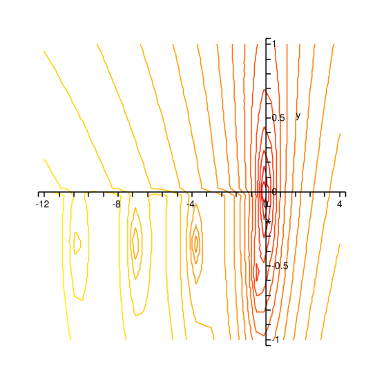
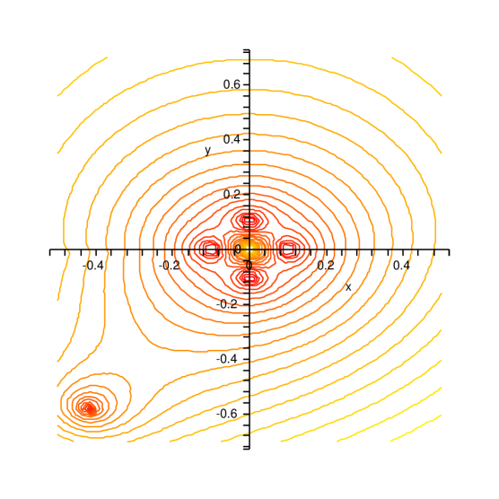
Figure 3: These plots, generated by the Maple 9.5 software package, show as poles the roots of the consistency relation when $\mu=m=0$ and $\beta=0.01$. They are contour plots of the logarithm of the absolute value of the l.h.s. of Eq. (41). The roots near the origin can be determined by Maple’s root finding routine as $\pm(0.0997-1.40\times 10^{-4}i)$ and $\pm 0.100i$.

The right hand plot shows the roots near the origin already calculated analytically. There are also other roots, one at $-0.419-0.577i$ and a sequence with almost identical imaginary parts of $-0.355i$ exactly analogous to those found by Seahra Seahra .

V.4 Massive brane field

Let us now consider the case were $\mu\gg\beta^{2}$ where we are still considering $\beta\ll 1$. When $\beta=0$ there are roots to Eq. (41) at ${\hat{\rho}}=\pm\mu$. When $\beta\neq 0$ we can work out how these are perturbed. By writing ${\hat{\rho}}=\mu+\delta{\hat{\rho}}$ we can expand the consistency relation by a Taylor series about ${\hat{\rho}}=\mu$ to get the lowest order correction

$$\delta{\hat{\rho}}=\frac{\beta^{2}\,H_{\nu}^{(1)}(\mu)}{4\mu\Big{(}\mu H_{\nu-1}^{(1)}(\mu)+(2-\nu)H_{\nu}^{(1)}(\mu)\Big{)}}.$$ (66)

So the roots are

$${\hat{\rho}}\approx\pm\left(\mu+\frac{\beta^{2}\,H_{\nu}^{(1)}(\mu)}{4\mu\Big{(}\mu H_{\nu-1}^{(1)}(\mu)+(2-\nu)H_{\nu}^{(1)}(\mu)\Big{)}}\right),$$ (67)

and the frequency $\omega$ will be given by the dispersion relation (36).

One case of special interest is when $m=0$, where this simplifies to

$${\hat{\rho}}\approx\pm\left(\mu+\frac{\beta^{2}}{4\mu^{2}}\frac{H_{2}^{(1)}(\mu)}{H_{1}^{(1)}(\mu)}\right)\,.$$ (68)

The imaginary part always has the opposite sign to the real part. We can use the well known asymptotic behaviour of Bessel functions GradRyz to write

$$\Im\left(\frac{H_{2}^{(1)}(\mu)}{H_{1}^{(1)}(\mu)}\right)\sim\left\{\begin{array}[]{l@{\qquad}l}-\frac{\pi}{2}\mu&\mu\to 0\\ -1&\mu\to\infty\end{array}\right.$$ (69)

so for a light field on the brane, where $\beta\ll\mu\ll 1$

$${\hat{\rho}}\approx\pm\left(\mu-\frac{\pi\beta^{2}}{8\mu}\,i\right)\,,\qquad\omega\approx\pm\sqrt{k^{2}+\mu^{2}}-\frac{\pi\beta^{2}}{8\sqrt{k^{2}+\mu^{2}}}\,i\,.$$ (70)

There is also a solution with purely imaginary ${\hat{\rho}}$ which corresponds to the tachyonic bound state.

VI Conclusions

In this paper we have investigated the behaviour of a boundary field theory on a Minkowski brane linearly coupled to a bulk field in anti-de Sitter spacetime. We have calculated an instability criterion for the coupled boundary and bulk oscillators. Above a critical coupling $\beta_{\rm crit}=\sqrt{2(\nu-2)\mu^{2}/\ell}$ there is a state with a purely imaginary effective mass. This state is spatially bounded and normalizable in the bulk, and describes a tachyonic instability on large-scales (small $k$). When either field is massless $\beta_{\rm crit}=0$, so that the instability will always occur for non-zero coupling. Below the critical coupling there is no tachyonic state and no bound state, in contrast to the case of a Minkowski bulk George . Instead we find quasi-normal modes.

The quasi-normal modes describe the late-time behaviour of the system when there is no tachyonic instability. For weak coupling, there is a quasi-normal mode which represents a very slowly decaying oscillatory solution. For instance in the low energy limit ($m\ell\ll 1$) we find a decay time of the order $(m\ell)^{-1}m^{-1}$. This contradicts the conjecture of Cartier and Durrer CD04 that orbifold boundary theories necessarily have instabilities. It is necessary to impose a physical boundary condition in order to determine which poles in the complex frequency plane describe the behaviour of the system. Quasi-normal modes are determined by a purely outgoing condition at infinity and thus only poles in the lower half complex plane describe the late-time evolution of the system.

Quasi-normal modes are not normalizable modes. For the classical problem normalizability is not a concern because the quasi-normal mode solution is only valid in the causal future development of the brane (see Ref. Szpak for a dicussion). On the other hand normalisability is a concern if one wishes to construct an initial quantum vacuum in terms of independent oscillators with finite action. In contrast to the work of George in a Minkowski bulk George we are not able to give the full spectrum of the quantum vacuum state below the critical coupling.

When the coupling is zero, a massless bulk field behaves in a way very similar to gravitational waves in the Randall–Sundrum brane-world RS99 . There is a massless zero mode solution on the brane and a spectrum of massive Kaluza–Klein states. In addition, there is a spectrum of quasinormal modes found by Seahra Seahra which describe the evolution of the gravity waves at intermediate times on the brane, though the zero mode dominates at late times. When a non-zero coupling is introduced this behaviour is modified dramatically. The zero mode, ${\hat{\rho}}=0$, is no longer a solution but is perturbed to solutions with complex ${\hat{\rho}}$. Without the coupling, the boundary condition at the brane is purely Neumann, thereby admitting a bounded zero-mode. One can think of the coupling as mixing Dirichlet and Neumann boundary conditions. A similar effect could occur with a moving boundary, such as an expanding brane universe.

An important difference in the case of gravitational perturbations in the bulk is that these are not in general coupled to linear matter perturbations on the brane and metric backreaction is treated as a second-order effect. An important exception is the case of fluctuations in an inflaton field driving inflation on a brane. Inflaton fluctuations on the brane are linearly coupled to bulk metric perturbations. These fluctuations start on small scales where they are strongly coupled to bulk gravitational perturbations KLMW . Thus, we must specify the vacuum state for a coupled boundary (inflaton fluctuations) and bulk (metric perturbations) system YK .

In order to address this issue, we need to extend our analysis to the case of a de Sitter brane. Due to the curvature of a de Sitter brane, there appears a mass gap GS in the spectrum of the free bulk field and there arises the possibility of having stable massive bound states in the mass gap LS . One could crudely model the existence of a cosmological horizon in de Sitter space by imposing an infra-red cut-off on wavelengths larger than the Hubble length, suppressing the tachyonic instability for sufficiently small coupling or large Hubble rate. We leave a full analysis of the de Sitter brane for future work but it is intriguing to note that a de Sitter brane might provide a good model for a coupled brane-bulk quantum field theory, where a Minkowski brane does not.

References

- (1) L. Randall and R. Sundrum, Phys. Rev. Lett. 83, 4690 (1999) [arXiv:hep-th/9906064].
- (2) For a review, see R. Maartens, Liv. Rev. Rel. 7, 1 (2004) [arXiv:gr-qc/0312059].
- (3) R. Maartens, D. Wands, B. A. Bassett and I. Heard, Phys. Rev. D 62, 041301 (2000) [arXiv:hep-ph/9912464].
- (4) K. Koyama, D. Langlois, R. Maartens and D. Wands, JCAP 0411, 002 (2004) [arXiv:hep-th/0408222].
- (5) S. L. Dubovsky, V. A. Rubakov and P. G. Tinyakov, Phys. Rev. D62, 105011 (2000).
- (6) Y. Himemoto, T. Tanaka and M. Sasaki, Phys. Rev. D 65 (2002) 104020 [arXiv:gr-qc/0112027].
- (7) D. Langlois and M. Sasaki, Phys. Rev. D 68 (2003) 064012 [arXiv:hep-th/0302069].
- (8) S. S. Seahra, arXiv:hep-th/0501175.
- (9) P. Binetruy, M. Bucher and C. Carvalho, Phys. Rev. D 70, 043509 (2004) [arXiv:hep-th/0403154].
- (10) C. Cartier and R. Durrer, arXiv:hep-th/0409287.
- (11) A. George, arXiv:hep-th/0412067.
- (12) I.S. Gradshteyn and I.M. Ryzhik Tables of Integrals, Series and Products, Sixth Ed. (2000) Academic Press, San Diego, USA
- (13) S. B. Giddings, E. Katz and L. Randall, JHEP 0003, 023 (2000) [arXiv:hep-th/0002091].
- (14) N. Szpak, arXiv:gr-qc/0411050
- (15) H. Yoshiguchi and K. Koyama, Phys. Rev. D 71 (2005) 043519 [arXiv:hep-th/0411056].
- (16) J. Garriga and M. Sasaki, Phys. Rev. D 62, 043523 (2000) [arXiv:hep-th/9912118].