Abstract

We study the $c_{L}=25$ limit, which corresponds to $c=1$ string theory, of bulk and boundary correlation functions of Liouville theory with FZZT boundary conditions. This limit is singular and requires a renormalization of vertex operators. We formulate a regularization procedure which allows to extract finite physical results. A particular attention is paid to $c=1$ string theory compactified at the self-dual radius $R=1$. In this case, the boundary correlation functions diverge even after the multiplicative renormalization. We show that all infinite contributions can be interpreted as contact terms arising from degenerate world sheet configurations. After their subtraction, one gets a well defined set of correlation functions. We also obtain several new results for correlation functions in Liouville theory at generic central charge.

1 Introduction

Non-critical string theories (see for instance [1, 2, 3] for a review) have long played the role of an interesting laboratory to test various phenomena of critical string theories. A recent breakthrough in the understanding of their non-perturbative effects [4, 5, 6, 7, 8, 9, 10, 11, 12, 13, 14, 15, 16, 17, 18, 19, 20, 21, 22, 23] drew a lot of attention to these theories. The ground for this breakthrough was prepared by a progress in Liouville theory, where two sets of conformally invariant boundary conditions, corresponding to the so called FZZT [24, 25] and ZZ branes [26], were discovered and all basic boundary correlation functions were calculated [27, 28, 29]. A review of these results can be found in [30].

Usually, the Liouville correlations functions are found for generic values of the Liouville central charge and they are represented as complicated combinations of (integrals of) some special functions. On the other hand, the most interesting non-critical string theory is the $c=1$ string theory. Besides giving the first non-trivial example of a non-rational CFT, it possesses a clear geometric interpretation as a string theory in a two-dimensional spacetime. It also allows for non-trivial backgrounds, such as the two-dimensional black hole, so that it might be useful in the analysis of black hole thermodynamics. Finally, it appears as a building block in many constructions of critical superstrings.

The field content of $c=1$ string theory consists of a massless scalar matter coupled with the Liouville field with central charge $c_{L}=25$. This is a very special value of the central charge for Liouville theory, since its correlation functions typically diverge at this point. This well known divergence is a counterpart of the fact that the $c=1$ CFT is a singular limit in the family of minimal $(p,q)$ models [31].

In this paper we demonstrate how it is possible to define all Liouville correlation functions in the $c_{L}=25$ limit systematically. The above mentioned divergence at $c_{L}=25$ can be removed by a multiplicative renormalization of the Liouville coupling constants. Whereas this is a straightforward procedure for the theory in the bulk, for the boundary correlation functions there are additional complications related to the appearance of the so called “contact terms”, which diverge even after the renormalization. In the simplest cases, these contact terms are entire functions of the boundary cosmological constants and therefore vanish after the insertion of a finite number of boundary cosmological constant operators. In the matrix model approach, such terms are usually considered as non-universal and excluded from the final results, and one can expect the same situation to occur in the CFT under consideration.

However, our analysis shows that there are other divergent contributions, which have a more complicated form and have no simple analogues in the matrix models. Nevertheless, we show that all of the divergent terms arising in the $c_{L}=25$ limit, independently of their form, can be interpreted as contributions coming from degenerate two-dimensional geometries, and they should therefore be excluded from the resulting expressions for the correlation functions. In this way one arrives at finite results for all basic correlators, which, once multiplied by the corresponding matter contributions, give the correlation functions of $c=1$ string theory.

Recently, an attempt to extract the $c_{L}=25$ limit of Liouville theory with boundary was made in [32]. However, the complication related to the appearance of the contact terms was not taken into account. As a result, [32] provided only divergent results for the leading non-universal contributions, whereas the physical part of the correlation functions remained non calculated. Our paper fulfills this gap and presents the physical results derived from a careful regularization procedure based on a consistent coupling of Liouville theory and matter CFT. As in [32], we limit our analysis to boundary conditions of FZZT type. The correlation functions on ZZ branes can be obtained by applying a well known relation between these two types of branes [5, 27, 11, 29, 33].

The singularity of the $c_{L}=25$ limit implies that the final results are simpler than those for generic values of the central charge. The greatest simplifications occur if one restricts oneself to the spectrum of vertex operators corresponding to $c=1$ string theory compactified at the self-dual radius $R=1$, which is the case considered in [32]. The reason is that in this case all operators are degenerate operators in both the matter and Liouville sectors. In particular, all special functions reduce to ordinary functions and all correlators can be given quite explicit expressions. Therefore, we will be primarily interested in this situation. The self-dual radius introduces additional singularities with respect to the generic case. We show that, after subtraction of the contact terms, our renormalization ensures that all correlation functions remain finite.

The restriction to the self-dual radius of compactification is also relevant for the link to topological strings. It has long been known that $c=1$ non-critical string theory compactified on a circle of radius $R=1$ provides a dual description of topological strings on the conifold [34, 35, 36, 37, 38]. One might therefore expect that the correlation functions that we study here shed light on the dynamics of some D-branes in topological string theory.

The organization of the paper is the following. In section 2 we recall some basic facts about Liouville theory, introduce our notations and collect the known results for the correlation functions of Liouville vertex operators on a sphere and on a disk. In section 3 we formulate our procedure to take the $c=1$ limit, based on a CFT representing Liouville theory coupled to matter with background charge. At this point we also introduce the multiplicative renormalization of the vertex operators. In the following two sections we compute sphere and disk correlation functions for $c_{L}=25$. The former are considered in section 4 and the latter are dealt with in section 5. Since in the case of boundary correlators the multiplicative renormalization is not enough to remove all divergences, we begin in subsection 5.1 by discussing the meaning of the contact terms and the necessity of excluding them from the results. We then proceed with the details of the computation in the remaining part of the section. Notice that, as an intermediate step in our derivation of the correlators in the $c_{L}=25$ limit, we also find the Liouville correlation functions for a generic central charge with momenta corresponding to degenerate matter fields, and these agree with the predictions of the microscopic approach found in [39]. Finally, we conclude in section 6 by summarizing the list of our main results. Readers who are not interested in the details of the derivations may find this list useful to get to the results of our work quickly. Several appendices present various details of our calculations.

2 Correlation functions in Liouville theory

Liouville theory arises when one considers two-dimensional quantum gravity, possibly coupled to matter, in the conformal gauge. It is defined by the following action:

$$S_{L}={1\over 4\pi}\int_{\Sigma}d^{2}z\,\sqrt{g}\left((\partial\phi)^{2}+Q\hat{R}\phi+4\pi\mu\,e^{2b\phi}\right).$$ (2.1)

It is a CFT whose central charge is given by

$$c_{L}=1+6Q^{2}$$ (2.2)

and the parameter $b$ in (2.1) is related to Q via the relation

$$Q=b+{1\over b}.$$ (2.3)

In general, $b$ and $Q$ are determined by the requirement that the total central charge of the Liouville and matter field is equal to $26$. For example, in the case when matter is represented by a minimal $(p,q)$ model with central charge $c_{p,q}=1-6{(p-q)^{2}\over pq}$, the relation (2.2) implies that $b=\sqrt{p/q}$. Coupling to $c=1$ matter corresponds to the limit $b=1$ so that the Liouville central charge becomes $c_{L}=25$.

2.1 Sphere correlation functions

An important class of conformal primaries in Liouville theory consists of the bulk operators

$$V_{\alpha}(z)=e^{2\alpha\phi(z)}\,,$$ (2.4)

whose scaling dimension is given by $\Delta_{\alpha}=\bar{\Delta}_{\alpha}=\alpha(Q-\alpha)$. In particular, the Liouville interaction in the action (2.1) can be seen as a perturbation of the Lagrangian by the cosmological constant operator $\delta{\cal L}=\mu V_{b}$.

In principle, all information about Liouville theory on a manifold with topology of a sphere is contained in the three-point correlation function, which was found to be [40, 41]

$$\langle V_{\alpha_{1}}(z_{1})V_{\alpha_{2}}(z_{2})V_{\alpha_{3}}(z_{3})\rangle_{\rm sphere}={C(\alpha_{1},\alpha_{2},\alpha_{3})\over|z_{12}|^{\,2(\Delta_{1}+\Delta_{2}-\Delta_{3})}|z_{23}|^{\,2(\Delta_{2}+\Delta_{3}-\Delta_{1})}|z_{31}|^{\,2(\Delta_{3}+\Delta_{1}-\Delta_{2})}},$$ (2.5)

where

$$C(\alpha_{1},\alpha_{2},\alpha_{3}) =\left[\pi\mu\gamma(b^{2})b^{2-2b^{2}}\right]^{\left(Q-\sum\alpha_{i}\right)/b}$$ (2.6)

$$\times{{\bf\Upsilon}_{b,0}{\bf\Upsilon}_{b}(2\alpha_{1}){\bf\Upsilon}_{b}(2\alpha_{2}){\bf\Upsilon}_{b}(2\alpha_{3})\over{\bf\Upsilon}_{b}(\alpha_{1}+\alpha_{2}+\alpha_{3}-Q){\bf\Upsilon}_{b}(\alpha_{1}+\alpha_{2}-\alpha_{3}){\bf\Upsilon}_{b}(\alpha_{2}+\alpha_{3}-\alpha_{1}){\bf\Upsilon}_{b}(\alpha_{3}+\alpha_{1}-\alpha_{2})}.$$

Here we used the standard notation for the di-gamma function

$$\gamma(x)={\Gamma(x)\over\Gamma(1-x)}\,,$$ (2.7)

while the other special functions appearing in (2.6) and in the following are defined in appendix A.

A particular important case of the three-point function is given by the two-point function. In Liouville theory it is also often interpreted as a reflection amplitude which is the coefficient $D_{\rm(refl)}(\alpha)$ appearing after the duality transformation $\alpha\to Q-\alpha$:

$$V_{\alpha}(z)=D_{\rm(refl)}(\alpha)V_{Q-\alpha}(z).$$ (2.8)

Its explicit expression reads

$$D_{\rm(refl)}(\alpha)=\left[\pi\mu\gamma(b^{2})\right]^{\left(Q-2\alpha\right)/b}{\gamma(2b\alpha-b^{2})\over b^{2}\,\gamma(2-2\alpha/b+1/b^{2})}.$$ (2.9)

However, in string theory and quantum gravity the correct way to define the two-point function is through the three-point correlator (2.6). As explained for instance in appendix C of [42], one should take the three-point function at the particular values of momenta $\alpha_{1}=\alpha_{2}$ and $\alpha_{3}=b$, and then integrate it once with respect to $-\mu$. This procedure allows to avoid any problems related to the residual gauge symmetry on the sphere with two insertions of the vertex operators. In this way one obtains

$$D(\alpha)=\left[\pi\mu\gamma(b^{2})\right]^{\left(Q-2\alpha\right)/b}{(Q-2\alpha)\gamma(2b\alpha-b^{2})\over\pi b^{2}\,\gamma(2-2\alpha/b+1/b^{2})}.$$ (2.10)

Thus, the two-point function found from the three-point correlator differs from the reflection amplitude by a factor:

$$D(\alpha)={Q-2\alpha\over\pi}\,D_{\rm(refl)}(\alpha).$$ (2.11)

In our study we have to use the function (2.10). In particular, after the renormalization only $D(\alpha)$ gives finite expressions for all momenta in the $c=1$ limit.

2.2 Disk correlation functions

When Liouville theory is formulated on a surface with boundary, there are two possible boundary conditions, respectively of Neumann and Dirichlet type. The first type gives rise to the so called FZZT branes [24, 25], while the second one leads to the ZZ branes [26]. In order to work with FZZT boundary conditions, one adds the following boundary contribution to the action (2.1):

$$S_{\rm bnd}={1\over 2\pi}\int_{\partial\Sigma}d\xi\,g^{1/4}\left(Q\hat{K}\phi+2\pi\mu_{{}_{B}}e^{b\phi}\right).$$ (2.12)

The boundary conditions are parameterized by the boundary cosmological constant $\mu_{{}_{B}}$. However, all correlation functions are more naturally written in terms of another parameter $s$, which is related to $\mu_{{}_{B}}$ through

$${\mu_{{}_{B}}}=\sqrt{\mu\over\sin(\pi b^{2})}\cosh(\pi bs).$$ (2.13)

In this theory, besides the bulk operators (2.4), there are operators acting on the boundary and changing the boundary conditions

$$B_{\beta}^{s_{1}s_{2}}(\xi)=e^{\beta\phi(\xi)}.$$ (2.14)

Here the labels $s_{1}$ and $s_{2}$ correspond to the boundary conditions to the left and right of the point $\xi$ on the boundary. The scaling dimension of the operator (2.14) is given by $\Delta_{\beta}=\bar{\Delta}_{\beta}=\beta(Q-\beta)$.

Let us now summarize the non-trivial correlation functions in the theory with boundary. We recall that definitions and properties of the special functions appearing below are summarized in appendix A.

• One-point bulk correlation function [24]

  $$\langle V_{\alpha}(z)\rangle_{\rm disk}={U(\alpha|s)\over|z-\bar{z}|^{2\Delta_{\alpha}}},$$ (2.15)

  $$U(\alpha|s)={1\over\pi b}\,[\pi\mu\gamma(b^{2})]^{(Q-2\alpha)/2b}\Gamma(2b\alpha-b^{2})\Gamma(2\alpha/b-1/b^{2}-1)\cosh\left((2\alpha-Q)\pi s\right).$$ (2.16)

• Bulk-boundary correlation function [27]

  $$\langle V_{\alpha}(z)B_{\beta}^{ss}(\xi)\rangle_{\rm disk}={R(\alpha,\beta|s)\over|z-\bar{z}|^{2\Delta_{\alpha}-\Delta_{\beta}}|z-\xi|^{2\Delta_{\beta}}},$$ (2.17)

  $$R(\alpha,\beta|s) =-2\pi i\left[\pi\mu\gamma(b^{2})b^{2-2b^{2}}\right]^{(Q-2\alpha-\beta)/2b}{\Gamma_{b}^{3}(Q-\beta)\Gamma_{b}(2\alpha-\beta)\Gamma_{b}(2Q-2\alpha-\beta)\over\Gamma_{b}(Q)\Gamma_{b}(Q-2\beta)\Gamma_{b}(\beta)\Gamma_{b}(Q-2\alpha)\Gamma_{b}(2\alpha)}$$

  $$\times\,\int\limits_{-i\infty}^{i\infty}dt\,e^{-2\pi ts}{{\bf S}_{b}(t+\beta/2+\alpha-Q/2){\bf S}_{b}(t+\beta/2-\alpha+Q/2)\over{\bf S}_{b}(t-\beta/2-\alpha+3Q/2){\bf S}_{b}(t-\beta/2+\alpha+Q/2)}.$$ (2.18)

• Three-point boundary correlation function [28]

  $$\langle B_{\beta_{3}}^{s_{1}s_{3}}(\xi_{1})B_{\beta_{2}}^{s_{3}s_{2}}(\xi_{2})B_{\beta_{1}}^{s_{2}s_{1}}(\xi_{3})\rangle_{\rm disk}={C(\beta_{1},\beta_{2},\beta_{3}|s_{1},s_{2},s_{3})\over|\xi_{12}|^{\Delta_{1}+\Delta_{2}-\Delta_{3}}|\xi_{23}|^{\Delta_{2}+\Delta_{3}-\Delta_{1}}|\xi_{31}|^{\Delta_{3}+\Delta_{1}-\Delta_{2}}},$$ (2.19)

  $$C(\beta_{1},\beta_{2},\beta_{3}|s_{1},s_{2},s_{3})=-4\pi i\left[\pi\mu\gamma(b^{2})b^{2-2b^{2}}\right]^{\left(Q-\sum\beta_{i}\right)/2b}$$

  $$\qquad\times\,{\Gamma_{b}(\beta_{2}+\beta_{3}-\beta_{1})\Gamma_{b}(2Q-\beta_{1}-\beta_{2}-\beta_{3})\Gamma_{b}(Q-\beta_{1}-\beta_{2}+\beta_{3})\Gamma_{b}(Q-\beta_{1}+\beta_{2}-\beta_{3})\over\Gamma_{b}(Q)\Gamma_{b}(Q-2\beta_{1})\Gamma_{b}(Q-2\beta_{2})\Gamma_{b}(Q-2\beta_{3})}$$

  $$\qquad\times\,{{\bf S}_{b}\left(Q-\beta_{3}+i{s_{1}-s_{3}\over 2}\right){\bf S}_{b}\left(Q-\beta_{3}-i{s_{1}+s_{3}\over 2}\right)\over{\bf S}_{b}\left(\beta_{2}+i{s_{2}-s_{3}\over 2}\right){\bf S}_{b}\left(\beta_{2}-i{s_{2}+s_{3}\over 2}\right)}\int\limits_{-i\infty}^{i\infty}dt\,\prod\limits_{i=1}^{4}{{\bf S}_{b}(t+U_{i})\over{\bf S}_{b}(t+V_{i})},$$ (2.20)

  where

  $$\begin{array}[]{rclcrcl}U_{1}&=&Q+i{s_{1}+s_{2}\over 2}-\beta_{1},&&V_{1}&=&2Q+i{s_{2}-s_{3}\over 2}-\beta_{1}-\beta_{3},\\ U_{2}&=&Q-i{s_{1}-s_{2}\over 2}-\beta_{1},&&V_{2}&=&Q+i{s_{2}-s_{3}\over 2}-\beta_{1}+\beta_{3},\\ U_{3}&=&i{s_{2}-s_{3}\over 2}+\beta_{2},&&V_{3}&=&Q+is_{2},\\ U_{4}&=&Q+i{s_{2}-s_{3}\over 2}-\beta_{2},&&V_{4}&=&Q.\\ \end{array}$$ (2.21)

Several comments are in order. First of all, one should give a precise definition of the contours of integration in (2.18) and (2.20). The rule is the following: for both integrals, the integration contour in the complex $t$-plane lies on the right of the poles of the integrand coming from poles of the numerator and to the left of the poles coming from zeros of the denominator. This gives an unambiguous definition of the integrals, except in the case when a pole from the numerator coincides with a pole from the denominator. If such a situation of colliding poles occurs, it means that the integral has a singularity at the corresponding point in the parameter space.

Another comment is that we have changed the overall normalization of the one-point bulk and the three-point boundary correlation functions with respect to the one usually found in the literature. Compared to the standard expressions from [24] and [28], the first one is divided by $2\pi$ and the second one is multiplied by $4\pi$. This is done because the theory is completely defined by the bulk-boundary and the three-point correlation functions, whereas the one-point bulk correlator is a derived quantity, whose normalization can be fixed starting from any of the two. For example, one can take the bulk-boundary correlation function (2.18) with the boundary operator being the boundary cosmological constant operator, i.e. $\beta=b$, and then integrate with respect to $-\mu_{{}_{B}}$. In appendix B, we show that this procedure gives precisely (2.16) with the factor $1/2\pi$ included. This factor can be traced back to the rotational symmetry of the disk, which remains non-fixed in the one-point correlator. The correct normalization valid for string theory requires to divide by the volume of the gauge group and thus follows from the bulk-boundary correlation function where all symmetries are fixed.

However, a similar procedure (see below) done for the standard expression for the three-point function leads to a result differing by a factor $4\pi$. This means that there is a mismatch between the bulk-boundary and the three-point functions. Assuming that the bulk-boundary correlator is correct, one should then modify the standard expression for the three-point correlator by including this factor, as we did in (2.20).

The third comment is that, similarly to the bulk case, one can also consider the two-point boundary correlation function. Its usual definition used in Liouville theory is through the reflection relation [24]

$$B_{\beta}^{s_{1}s_{2}}(\xi)=d_{\rm(refl)}(\beta|s_{1},s_{2})\,B_{Q-\beta}^{s_{1}s_{2}}(\xi),$$ (2.22)

where

$$d_{\rm(refl)}(\beta|s_{1},s_{2})={\left[\pi\mu\gamma(b^{2})b^{2-2b^{2}}\right]^{(Q-2\beta)/2b}\Gamma_{b}(2\beta-Q)\Gamma_{b}^{-1}(Q-2\beta)\over{\bf S}_{b}\left(\beta+i{s_{1}+s_{2}\over 2}\right){\bf S}_{b}\left(\beta-i{s_{1}+s_{2}\over 2}\right){\bf S}_{b}\left(\beta+i{s_{1}-s_{2}\over 2}\right){\bf S}_{b}\left(\beta-i{s_{1}-s_{2}\over 2}\right)}.$$ (2.23)

However, as usual, the two-point function relevant for quantum gravity should be obtained through the three-point function (2.20) by the standard procedure of taking one of the operators to be the boundary cosmological constant operator and integrating with respect to $-\mu_{{}_{B}}$. In fact, since the initial expression is not explicitly symmetric, there are three inequivalent ways to do this depending on which operator we choose to represent $B_{b}^{ss}$. In appendix C we show that all three ways lead to the same result. This fact provides a non-trivial explicit check of the symmetry of the three-point function (2.20) under cyclic permutations of its arguments. We find that, as in the bulk case (2.11), the two-point function differs from the reflection amplitude (2.23) by a simple (momentum dependent) factor

$$d(\beta|s_{1},s_{2})={2(Q-2\beta)}\,d_{\rm(refl)}(\beta|s_{1},s_{2}).$$ (2.24)

In appendix C.3, starting from the two-point function found in this way, we also rederive the one-point function of the cosmological constant operator. The result should coincide with the one obtained from the bulk-boundary correlator, and this forced us to introduce the $4\pi$ factor mentioned above. These results also contain information about the one-point function of the boundary cosmological constant operator which is found to be

$$W(s)={2b\,\over\pi}\left[\pi\mu\gamma(b^{2})\right]^{{1\over 2b^{2}}}\Gamma\left(2-{1\over b^{2}}\right)\,\cosh(\pi s/b).$$ (2.25)

This quantity will be quite important in the following so it is useful to give its explicit expression at this point.

3 The $c=1$ limit

3.1 2D string theory with a background charge

It is well known that the $c=1$ limit of the family of CFTs with central charge $c\leq 1$ coupled to Liouville theory with $c_{L}=26-c$ is singular. Therefore, one cannot put directly $b=1$ in the results obtained in Liouville theory with a generic central charge. To make the limit meaningful, we perform a regularization by considering Liouville theory coupled to a Gaussian matter field with a background charge $q$, following [39, 43]. The Gaussian field is described by the following action

$$S_{\rm mat}={1\over 4\pi}\int_{\Sigma}d^{2}z\,\sqrt{g}\left((\partial x)^{2}+iqx\hat{R}\right)+{1\over 2\pi}\int_{\partial\Sigma}d\xi g^{1/4}\left(iqx\hat{K}\right).$$ (3.1)

The background charge leads to a shift of the central charge of the matter field

$$c_{\rm mat}=1-6q^{2}.$$ (3.2)

Requiring that the total central charge of the system vanishes

$$c_{\rm tot}=c_{L}+c_{\rm mat}+c_{\rm ghost}=\left(1+6Q^{2}\right)+\left(1-6q^{2}\right)-26=0,$$ (3.3)

one can express the background charge in terms of the Liouville parameter $b$

$$q={1\over b}-b.$$ (3.4)

The bulk and boundary vertex operators of the full theory

$${\cal V}_{p}=e^{-ipx}e^{2\alpha(p)\phi},\qquad{\cal B}_{p}=e^{-ipx}e^{\beta(p)\phi}$$ (3.5)

are found from the condition that their dimensions are equal to 1

$$\Delta\left[{\cal V}_{p}\right] = {p\over 2}\left({p\over 2}+q\right)+{\alpha}\left(Q-{\alpha}\right)=1,$$ (3.6)

$$\Delta\left[{\cal B}_{p}\right] = {p}\left(p+q\right)+{\beta}\left(Q-{\beta}\right)=1.$$ (3.7)

Taking into account the Seiberg bound [44], this gives for the parameters $\alpha$ and $\beta$

$$\begin{array}[]{llll}\alpha(p)=b-p/2&{\rm\ if\ \ }p>-q,&\quad\alpha(p)=1/b+p/2&{\rm\ if\ \ }p<-q,\\ \beta(p)=b-p&{\rm\ if\ \ }p>-q/2,&\quad\beta(p)=1/b+p&{\rm\ if\ \ }p<-q/2.\end{array}$$ (3.8)

The two branches of the solution correspond to the left and right moving (or positive and negative chirality) tachyons in the target space picture of two-dimensional string theory.

In order to restrict ourselves to the spectrum of the theory compactified at radius $R$, we have to take the discrete set of operators with quantized momenta

$$p_{n}={n/R}.$$ (3.9)

Then for $n\geq 0$ the corresponding Liouville momenta are

$$\alpha_{n}=b-{n\over 2R},\qquad\beta_{n}=b-{n\over R}.$$ (3.10)

In fact, for generic $R$ and $n\neq 0$, the correlation functions do not exhibit singularities. Therefore, the details of the limiting procedure are not important in this situation.

However, if $R$ is rational some additional singularities appear so that the $c=1$ limit should be treated with a great care. We will pay special attention to the case of the self-dual radius $R=1$. On the one hand, it is the most singular case, but on the other hand it allows the most explicit representation for the correlation functions. The origin of the additional divergences can be traced back to the fact that all operators with momenta $p_{n}=n$ are Liouville dressed degenerate matter fields of the $c=1$ CFT. Therefore, it is natural to take the $c=1$ limit in such a way that the operators in question are degenerate for all $b$. For general $b$ the momenta corresponding to the bulk degenerate fields are

$$p_{r,s}^{\rm bulk}=-q+r/b-sb,\qquad\alpha_{r,s}=Q/2-\left|{r\over 2b}-{sb\over 2}\right|,$$ (3.11)

and those of the boundary degenerate fields are

$$p_{r,s}^{\rm bnd}=\left(-q+r/b-sb\right)/2,\qquad\beta_{r,s}=Q/2-\left|{r\over 2b}-{sb\over 2}\right|,$$ (3.12)

where in both cases $r,s\in{\rm\bf Z},\ rs\geq 0$. Thus, when dealing with the case $R=1$, in the regularized theory we will set $R=b$ so that $p_{n}=n/b$ and the Liouville momenta (3.10) take the form

$$\alpha_{n}=b-{n\over 2b},\qquad\beta_{n}=b-{n\over b},\qquad n\geq 0.$$ (3.13)

This corresponds to the choice $r=n+1,\ s=1$ for the bulk and $r=2n+1,\ s=1$ for the boundary momenta.

However for $n<0$ this solution does not work. To get degenerate fields with momenta of the form (3.9), one has to choose $R=1/b$ and, for example, in the bulk case $r=1,\ s=1-n$ so that $p_{n}=nb$. This reflects difficulties in compactifying a field with a background charge. After compactification, there are degenerate fields only of either positive or negative chirality. On the other hand, to write non-vanishing correlation functions, one needs to satisfy the momentum conservation law in the matter sector, which due to the presence of the background charge $q$ acquires an additional term. For the sphere and disk correlation functions it takes respectively the following form

$$\sum\limits_{i=1}^{k}p^{\rm bulk}_{i}=-2q,\qquad\sum\limits_{i=1}^{k}p^{\rm bulk}_{i}+\sum\limits_{i=1}^{l}p^{\rm bnd}_{i}=-q.$$ (3.14)

This implies that at least one momentum must have $r,s\leq 0$ and hence must not be of the form (3.9) required by compactification. Thus, strictly speaking, we have a compactified theory only in the case $b=1$.

Usually, there are several ways to satisfy the conservation condition (3.14) which differ by the choice of chiralities of the vertex operators. In the $b=1$ limit they correspond just to different choices of signs of momenta and should lead to the same results. We are then free to choose a simple convention consisting in taking all operators except one to be of positive chirality. In addition, on the disk we will always choose a boundary operator to be the one with negative chirality. Then, if for positive chirality $p^{\rm bulk}_{i}=n_{i}/b$ and $p^{\rm bnd}_{i}=m_{i}/b$, the remaining momentum must be of the form

$$p^{\rm bulk}_{k}=-2q-n/b,\qquad p^{\rm bnd}_{l}=-q-m/b,$$ (3.15)

where $n=\sum_{i=1}^{k-1}n_{i}$ and $m=\sum_{i=1}^{k}n_{i}+\sum_{i=1}^{l-1}m_{i}$, respectively on the sphere and on the disk. The momenta (3.15) are also degenerate and can be obtained from (3.11) and (3.12) for $r=-(n+1),\ s=-1$ and $r=-(2m+1),\ s=-1$, respectively. Starting from the momenta (3.15) for the matter part, one arrives at the same Liouville momenta as in (3.13).

We conclude that, after fixing all Liouville momenta to be of the form (3.13), the only remaining free parameter in our system is $b$. We are interested in the limit $b\to 1$ where we should find the compactified $c=1$ string theory. In order to take this limit, we put $b=1-\varepsilon$ for a small parameter $\varepsilon$ and extract all singular and finite terms in the correlation functions. We will explain that the singular contributions are given by the so called contact terms, which are to be neglected, while the physical answers are only contained in the finite part of the correlation functions. The exact meaning of the contact terms will be explained in section 5.1.

3.2 Renormalization of couplings and vertex operators

It is known that to get a finite sensible $c=1$ limit, one should simultaneously renormalize the couplings of the theory (see for example [5, 45]). The basic Liouville couplings are renormalized as follows

$${\hat{\mu}}=\pi\gamma(b^{2})\mu,\qquad{\hat{\mu}_{{}_{B}}}={\pi\mu_{{}_{B}}\over\Gamma(1-b^{2})}.$$ (3.16)

The normalization is chosen so that the parameterization of the renormalized boundary cosmological constant looks simply as

$${\hat{\mu}_{{}_{B}}}=\sqrt{{\hat{\mu}}}\cosh(\tau),$$ (3.17)

where we introduced a new parameter

$$\tau=\pi bs.$$ (3.18)

The introduction of the parameter $\tau$ is very convenient. It allows to avoid complications related to the fact that, although in the $c=1$ limit the parameter $b$ disappears from (3.18), it is important to keep track of it to correctly derive the physical part of the correlation functions in the boundary theory. Another useful notation, which we will extensively use, is

$$\hat{\mu}_{ij}={\hat{\mu}_{{}_{B}}}(\tau_{i})-{\hat{\mu}_{{}_{B}}}(\tau_{j}).$$ (3.19)

The definitions (3.16) imply the renormalization of the bulk and boundary cosmological constant operators. We will show that, in order to get finite correlation functions at $R=1$, one should renormalize also all other vertex operators. Generalizing (3.16) and following [39, 43, 46], where the multiplicative renormalization was used to compare the CFT results with results of the discrete approach to 2D quantum gravity, we define the renormalized bulk and boundary operators with momentum $p$ as follows

$$\hat{\cal V}_{p}={1\over\pi\gamma(\alpha^{2}(p)-p^{2}/4)}\,{\cal V}_{p},\qquad\hat{\cal B}_{p}={\Gamma(1-\beta^{2}(p)+p^{2})\over\pi}\,{\cal B}_{p},$$ (3.20)

where the Liouville momenta $\alpha(p)$ and $\beta(p)$ were defined in (3.8). Their explicit expressions depend on the sign of $p$ and thus operators of positive and negative chirality have different renormalization factors:

$$\hat{\cal V}_{p}^{+}={1\over\pi\gamma(b^{2}-bp)}\,{\cal V}_{p}^{+},\qquad\hat{\cal B}_{p}^{+}={\Gamma(1-b^{2}+2bp)\over\pi}\,{\cal B}_{p}^{+},$$ (3.21)

and

$$\hat{\cal V}_{p}^{-}={1\over\pi\gamma(1/b^{2}+p/b)}\,{\cal V}_{p}^{-},\qquad\hat{\cal B}_{p}^{-}={\Gamma(1-1/b^{2}-2p/b)\over\pi}\,{\cal B}_{p}^{-}.$$ (3.22)

Notice that the renormalization factors for different chiralities become the same in the $b=1$ limit when expressed as functions of Liouville momenta.

The renormalized correlation functions are defined in terms of vertex operators $\hat{\cal V}_{p}$ and $\hat{\cal B}_{p}$

$$\hat{\cal A}\left(\{p_{i}^{\rm bulk}\},\{p_{j}^{\rm bnd}\}|\{s_{j}\}\right)=\left\langle\prod\limits_{i}\hat{\cal V}_{p_{i}^{\rm bulk}}(z_{i})\prod\limits_{j}\hat{\cal B}_{p_{j}^{\rm bnd}}^{\,s_{j+1}s_{j}}(\xi_{j})\right\rangle$$ (3.23)

and can be obtained from the non-renormalized expressions by multiplying them with the factors in (3.20). The correlation functions of the $c=1$ theory are found then in the limit $b\to 1$

$${\cal A}_{\,c=1}\left(\{p_{i}^{\rm bulk}\},\{p_{j}^{\rm bnd}\}|\{s_{j}\}\right)=\mathop{\lim}\limits_{b\to 1}\hat{\cal A}\left(\{p_{i}^{\rm bulk}\},\{p_{j}^{\rm bnd}\}|\{s_{j}\}\right).$$ (3.24)

Actually, in this paper we will consider only the Liouville part of the correlation functions. However, especially in the boundary case, this is the main non-trivial part which contains all information about the dependence on the boundary cosmological constant.

It is clear that in the limit $b\to 1$ the renormalization factors of both bulk and boundary cosmological constants appearing in (3.16) vanish, whereas for $p_{n}$ with $n>0$ (see (3.21)) the corresponding factors diverge as ${\varepsilon^{-1}}$ in the bulk case and remain finite for the couplings of the boundary operators. The necessity of a renormalization with such properties can be understood as follows. First, the analysis of sphere correlation functions fixes the renormalization of all bulk operators, which can also be confirmed by the fact that it gives a finite result for the one-point bulk correlator on a disk. Then, the renormalization of the boundary operators follows from the study of the bulk-boundary function and can be verified by analyzing the boundary two- and three-point functions. In the next sections we will study in detail all basic correlation functions of Liouville theory following this sequence.

4 Sphere correlation functions in the $c=1$ limit

First, we evaluate the $c_{L}=25$ limit of the bulk correlation functions for Liouville theory on a sphere. The main quantity to consider is the three-point function (2.6). For the momenta (3.10) it takes the form

$$C(\alpha_{n_{1}},\alpha_{n_{2}},\alpha_{n_{3}}) = \left[\pi\mu\gamma(b^{2})b^{2-2b^{2}}\right]^{{1\over b^{2}}+{1\over 2bR}\sum n_{i}-2}$$

$$\times{{\bf\Upsilon}_{b}(b){\bf\Upsilon}_{b}\left(2b-{n_{1}\over R}\right){\bf\Upsilon}_{b}\left(2b-{n_{2}\over R}\right){\bf\Upsilon}_{b}\left(2b-{n_{3}\over R}\right)\over{\bf\Upsilon}_{b}\left(2b-{1\over b}-{n_{1}+n_{2}+n_{3}\over 2R}\right){\bf\Upsilon}_{b}\left(b+{n_{3}-n_{1}-n_{2}\over 2R}\right){\bf\Upsilon}_{b}\left(b+{n_{1}-n_{2}-n_{3}\over 2R}\right){\bf\Upsilon}_{b}\left(b+{n_{2}-n_{3}-n_{1}\over 2R}\right)}.$$

This expression can be simplified if one takes into account the momentum conservation (3.14) from the matter sector, which implies that $n_{3}=n_{1}+n_{2}$. We also apply here the multiplicative renormalization (3.20). As explained in the previous section, our convention is to choose two operators of positive chirality and one of negative chirality, which in this case has to be the third one due to the just mentioned condition on $n_{i}$. Thus, the expression (4) must be multiplied by two factors from (3.21) and one from (3.22). As a result, it reduces to

$$\hat{C}(\alpha_{n_{1}},\alpha_{n_{2}},\alpha_{n_{1}+n_{2}})={{\hat{\mu}}^{{1\over b^{2}}+{n_{1}+n_{2}\over bR}-2}\over\pi^{3}b}.$$ (4.2)

The $b=1$ limit of this three-point function is well defined and gives

$$C_{c=1}(\alpha_{n_{1}},\alpha_{n_{2}},\alpha_{n_{1}+n_{2}})={1\over\pi^{3}}\,{\hat{\mu}}^{{n_{1}+n_{2}\over R}-1}.$$ (4.3)

One can show that for other choices of chiralities and for generic central charge the result differs from (4.2) only by a power of $b$ and hence it leads to the same expression (4.3) in the $c=1$ limit. This shows that our definition of the $c=1$ limit does not depend on the artifact of the choice of chiralities.

As explained above, the two-point function is obtained from the three-point correlator by putting one of the Liouville momenta equal to $b$ ($n=0$) and integrating with respect to (minus) the cosmological constant. For (4.3) this procedure gives

$$D_{c=1}(\alpha_{0})=-{1\over\pi^{3}}\,\log{\hat{\mu}},\qquad\ \ D_{c=1}(\alpha_{n})=-{R\over\pi^{3}n}\,{\hat{\mu}}^{n\over R},\quad n\geq 1.$$ (4.4)

Of course, the same results can be found from the explicit expression (2.10) for the two-point function at generic central charge.

Notice also that, if we had used the reflection amplitude $D_{\text{(refl)}}(\alpha)$ given in (2.9) as a starting point, instead of the two-point function derived from the three-point correlator, the computation in this subsection would have yielded a divergent result for $D_{c=1}(\alpha_{0})$. This provides a confirmation of the fact that the two-point function that we use is the one which is relevant for $c=1$ string theory.

To conclude, we see that the renormalization (3.20) is sufficient to produce finite results for sphere correlators in the $b=1$ limit. The result is analytic in the compactification radius $R$ and there are no additional singularities arising at the self-dual point.

5 Disk correlation functions in the $c=1$ limit

5.1 Divergent contributions as contact terms

Let us now turn to the correlation functions characterizing the theory on the disk with FZZT boundary conditions. In our analysis we will encounter a new phenomenon. It turns out that all correlation functions in the boundary theory at the self-dual compactification radius $R=1$, even after the multiplicative renormalization (3.20) of the bulk and boundary vertex operators, are divergent in the $c=1$ limit. However, we are now going to argue that the divergent contributions have the interpretation of contact terms, namely degenerate world sheet configurations, and should be omitted from the physical answers. In order to understand the nature of the divergences, it is useful to anticipate here the general structure of the correlation functions in the $c=1$ limit, which will be studied in full detail in the following subsections.

First, it is very easy to characterize the correlation functions of operators with only vanishing boundary momenta of the matter part. As we will see, in this case the leading term diverges as $1/\varepsilon$ and is an entire (polynomial) function of the boundary cosmological constants. Such terms are well known in the matrix approach to non-critical strings where they are called non-universal contributions and usually neglected. This is justified by the fact that they vanish after a finite number of differentiations with respect to $\mu_{{}_{B}}$, which means that such contributions disappear from the correlation functions with enough number of insertions of the boundary cosmological constant operators. In addition, since such terms are entire functions of $\mu_{{}_{B}}$, they do not contribute to correlation functions with ZZ boundary conditions, which can be obtained from non-trivial monodromy properties of correlators with FZZT conditions [11, 33, 45].

The meaning of these non-universal contributions becomes clear when one passes to the length representation of correlation functions [47, 48]. Suppose we have a correlation function $C(\mu_{{}_{B}})$ on the disk with FZZT boundary conditions described by the boundary cosmological constant $\mu_{{}_{B}}$. The parameter $\mu_{{}_{B}}$ is conjugated to the length of the boundary, and the correlation function can then be thought as a Laplace transform of the corresponding correlation function with a fixed boundary length

$$C(\mu_{{}_{B}})=\int\limits_{0}^{\infty}d\ell\,e^{-\,\ell\,\mu_{{}_{B}}}\,\tilde{C}(\ell)\,.$$ (5.1)

Let us concentrate on a contribution to $C(\mu_{{}_{B}})$ which is polynomial in $\mu_{{}_{B}}$. Applying the inverse Laplace transform, one finds that it contributes to $\tilde{C}(\ell)$ only at $\ell=0$:

$$\int\limits_{-i\infty}^{i\infty}d\mu_{{}_{B}}\,e^{-\,\ell\,\mu_{{}_{B}}}\,P(\mu_{{}_{B}})\sim P(-\partial/\partial\ell)\,\delta(\ell)\,.$$ (5.2)

Thus, the contributions which are entire functions of the boundary cosmological constant correspond to contributions of degenerate world sheets with boundaries shrunken to a point, as shown in fig. 1. The same conclusion remains true if different segments of the boundary are characterized by different boundary cosmological constants. Such degenerate configurations should be excluded from the sum over two-dimensional geometries and, correspondingly, from the final result.

Figure 1: Degenerate world sheet configuration with shrinking boundary. It looks like a sphere with a puncture appearing at the place of the degenerating hole.

The case when a correlation function involves boundary operators with non-vanishing boundary momenta is more complicated. In this case there are divergent terms up to order $\varepsilon^{-n_{\rm tot}-1}$, where $n_{\rm tot}=\sum n_{i}$ is the total momentum of the boundary operators. The leading divergent terms are still polynomials in the boundary cosmological constants. It is these leading contributions that were calculated in [32], although our answers even for these terms are different from those of [32]. The reason for this discrepancy is that the $c=1$ limit requires to be carefully defined and cannot be taken without considering the consistency of the coupling between the matter part and the Liouville part.

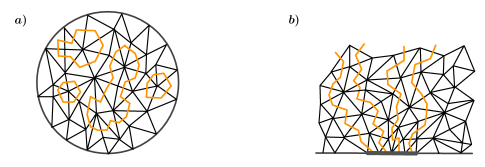
Figure 2: The loop gas representation of correlation functions in the SOS model. a) A typical contribution to the sum over triangulations. b) The loop gas representation of a boundary operator ($n=2$). In the continuum limit all lines come from the same single point of the boundary.

Subleading divergent terms are not entire functions anymore. Therefore, the previous reasoning based on (5.2), which allowed us to neglect the divergent contributions, cannot be directly applied and some additional argumentation is needed. A key observation is that the boundary correlation functions with momenta (3.13) can be written as polynomials in the one-point function $W(s)$ of the boundary cosmological constant operator, which was given in (2.25). This fact implies that all divergent terms come from the divergences of this function, and therefore one can remove all divergent contributions by renormalizing $W(s)$.

To understand the origin of this renormalization, it is useful to consider how these correlation functions are represented in the discrete approach to 2D quantum gravity. In this approach the system we are dealing with, namely Liouville theory coupled with a matter CFT, can be realized as the so called solid-on-solid (SOS) model on a fluctuating lattice. We are not going to present the SOS model here, and we refer the reader to [39] for the relevant details. What is important for us is the loop representation of this model [51, 49, 52], according to which the matter fields can be seen as non-intersecting loops on randomly triangulated surfaces. Correlation functions are given by a sum over all triangulations and all admissible configurations of the loops. A typical configuration contributing to the sum is shown in fig. 2a.

The degenerate boundary operators with momentum $p_{n}=n/b$ in the matter part are realized in the loop representation by the so called “star” operators, that create $2n$ lines at some point of the boundary (see fig. 2b). These lines are also non-intersecting and end at another point of the boundary. This fact allows to represent the general structure of the boundary correlation functions and was the starting point for their derivation from the discrete approach [53, 39].

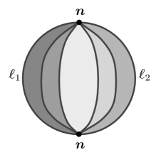
Figure 3: The two-point function $\tilde{d}_{n}(\ell_{1},\ell_{2})$.

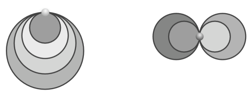
Figure 4: Possible degenerations of the two-point function. The first picture shows the case when the boundary of an external piece shrinks, whereas the second represents a degeneration of an internal sector. In both cases, the degenerate piece becomes a sphere growing from the marked point.

Let us then study in this context the structure of the correlation functions we are going to compute. The two-point function $d_{n}(\tau_{1},\tau_{2})$ of boundary operators with momenta $p_{n}$ is presented in fig. 3. One can see that $d_{n}$ is composed of the product of $2n$ two-point functions $d_{0}$ of operators with vanishing boundary momentum. The precise relation is easy to write in the $\ell$-representation due to the factorization property of the path integral measure [51, 52, 53]

$$\tilde{d}_{n}(\ell_{1},\ell_{2})=\int\limits_{0}^{\infty}d\ell^{\prime}_{1}\cdots d\ell^{\prime}_{2n}\,\tilde{d}_{0}(\ell_{1},\ell^{\prime}_{1})\,\tilde{d}_{0}(\ell^{\prime}_{1},\ell^{\prime}_{2})\,\cdots\,\tilde{d}_{0}(\ell^{\prime}_{2n},\ell_{2}).$$ (5.3)

From this representation one sees that singular contributions to $d_{0}$ give rise to singularities of $d_{n}$, and the latter can have a much more complicated form. However, we know that the divergent contributions to $d_{0}$ arise from degenerate world sheets. In fact, since $d_{n}$ can be represented as a polynomial in $W(\tau)$, all its singularities can be interpreted in terms of degenerate configurations of some of the $2n+1$ disks composing the initial world sheet. The possible degenerate configurations are shown on fig. 4, and correspond either to a disk with two coinciding marked points or to a pinched disk, together with a sphere growing from the marked point at the boundary. These contributions have again the interpretation of contact terms and should be neglected. Our analysis suggests that, in order to eliminate all of these contact terms, it is sufficient to remove the ones appearing in the correlation functions with vanishing momenta corresponding to each portion of the disk in fig. 3. We will see in subsection 5.4 that this is indeed the case.

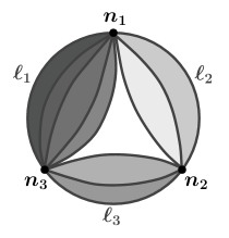
Figure 5: The three-point function $\tilde{C}_{n_{1},n_{2},n_{3}}(\ell_{1},\ell_{2},\ell_{3})$.

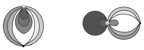
Figure 6: Possible degenerations of the three-point function. The two cases correspond to shrinking of the boundary of an external or an internal sector, respectively. The degenerate piece appears as a sphere attached to the point at the boundary where two of the three boundary operators collide.

A similar analysis can be applied to the case of the three-point function $C_{n_{1},n_{2},n_{3}}(\tau_{1},\tau_{2},\tau_{3})$. The representation in terms of non-intersecting lines is shown in fig. 5. We again see that the initial correlation function is reduced to a product of two- and three-point correlators with vanishing momenta. This is the origin of the representation of $C_{n_{1},n_{2},n_{3}}$ in terms of $W(\tau)$ that we will find below, and allows to interpret each divergent contribution as a result of the degeneration of some of the disks which divide the world sheet in fig. 5. The different possibilities are presented in fig. 6 and correspond to the same situations which we found in the case of the two-point function. Notice that one could expect the appearance of the degenerate configuration with all three marked points coinciding, which would give a world sheet in the form of a trefoil. However, one can show that the corresponding divergent term in $C_{0,0,0}$ vanishes.

One can finally analyze the bulk-boundary correlator in the same way. Its loop representation is depicted in fig. 7. In this case the lines corresponding to the boundary operator, instead of connecting two points of the boundary, end at the point where the bulk operator is inserted. The naive counting would then tell that the correlation function should diverge as $\varepsilon^{-n-m-1}$, but we will see in subsection 5.3 that only the $1/\varepsilon$ contribution is present. This can be explained from the fact, a consequence of (5.31) and (5.12), that all terms divergent as $\varepsilon^{-k}$ with $k>1$ in the boundary two-point function are proportional to $\left(\mu_{{}_{B}}(\tau_{1})-\mu_{{}_{B}}(\tau_{2})\right)^{k-1}$ and, therefore, vanish at $\mu_{{}_{B}}(\tau_{1})=\mu_{{}_{B}}(\tau_{2})$. Since the bulk operator cannot change the boundary conditions, the boundary cosmological constant indeed remains the same along the two boundaries of the disk formed by the outer lines coming from the two punctures. Thus, all contributions with a higher degree of divergence than $1/\varepsilon$ vanish. The remaining divergent contribution turns out to be a polynomial in $\mu_{{}_{B}}$, so it has the usual interpretation as contact term and has to be subtracted from the physical answer.

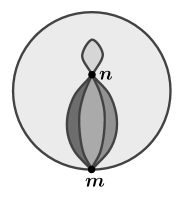
Figure 7: The bulk-boundary two-point function.

After we remove all divergent contributions which can be interpreted as contact terms, all correlation functions become finite. This is a non-trivial fact which shows the consistency of the proposed renormalization. We interpret the resulting finite expressions as physical results for the correlation functions in Liouville theory at $c_{L}=25$. Notice that, in the cases where a comparison is possible, they also agree with the corresponding results of the discrete approach obtained in [53, 39].

5.2 Bulk one-point function

First, we compute the simplest correlation function on the disk, namely the one-point bulk correlator (2.16). Substituting the expression for the Liouville momentum from (3.10) and replacing $s$ by $\tau$ using (3.18), one obtains

$$U(\alpha_{n}|\tau)={1\over\pi b}\,[\pi\mu\gamma(b^{2})]^{{1\over 2}\left({1\over b^{2}}-1+{n\over bR}\right)}\textstyle\Gamma\left(b^{2}-{nb\over R}\right)\Gamma\left(1-{1\over b^{2}}-{n\over bR}\right)\cosh\left(\left(1-{1\over b^{2}}-{n\over bR}\right)\tau\right).$$ (5.4)

Taking the limit $b\to 1$ and using the renormalization (3.21) corresponding to the case of positive chirality, one finds, for $n\geq 1$ and generic compactification radius $R$,

$$U_{c=1}(\alpha_{n}|\tau) =\mathop{\lim}\limits_{b\to 1}\left[{1\over\pi^{2}b}\,{\hat{\mu}}^{{1\over 2}\left({1\over b^{2}}-1+{n\over bR}\right)}\textstyle\Gamma\left(1-b^{2}+{nb\over R}\right)\Gamma\left(1-{1\over b^{2}}-{n\over bR}\right)\cosh\left(\left(1-{1\over b^{2}}-{n\over bR}\right)\tau\right)\right]$$

$$=-{{\hat{\mu}}^{n\over 2R}\over{\pi n\over R}\,\sin{\pi n\over R}}\,\cosh\left({n\tau\over R}\right).$$ (5.5)

The cases $R=1$ and $n=0$ should be treated separately. This can already be seen from the fact that the result (5.5) diverges at these values of the parameters. Let us start from the case of the self-dual radius with $n\neq 0$. The corresponding renormalized correlation function can be obtained from the first line in (5.5) substituting $R=b$. This gives

$$\hat{U}(\alpha_{n}|\tau)={1\over\pi^{2}b}\,{\hat{\mu}}^{{1\over 2}\left({n+1\over b^{2}}-1\right)}\Gamma\left(n+1-b^{2}\right)\textstyle\Gamma\left(1-{n+1\over b^{2}}\right)\cosh\left(\left(1-{n+1\over b^{2}}\right)\tau\right).$$ (5.6)

Substituting $b=1-\varepsilon$ and expanding in $\varepsilon$, one finds

$$\hat{U}(\alpha_{n}|\tau)\approx{(-1)^{n+1}\over 2\pi^{2}n}\,{\hat{\mu}}^{{n\over 2}}\left[\left({1\over(n+1)\varepsilon}+\log{\hat{\mu}}+c_{U}(n)\right)\cosh(n\tau)+2\tau\sinh(n\tau)\right]+O(\varepsilon),$$ (5.7)

where $c_{U}(n)$ is some $\tau$-independent function of $n$ which we are not interested in. We observe that, despite the renormalization, the correlation function still diverges. However, since $\cosh(n\tau)$ is a polynomial in $\cosh\tau$, the divergent term is a polynomial in the boundary cosmological constant ${\hat{\mu}_{{}_{B}}}$. As we explained in the previous subsection, such terms are interpreted as contact terms and correspond to degenerate world sheets. We then ignore them and take the “physical” one-point bulk correlation function in the $c=1$ limit to be just the last term in (5.7)

$${U^{(R=1)}_{c=1}(\alpha_{n}|\tau)}={(-1)^{n+1}\over\pi^{2}n}\,{\hat{\mu}}^{{n\over 2}}\,\tau\,\sinh(n\tau).$$ (5.8)

However, the case $n=0$ still remains singular. To get the correlation function in this situation, we return to the representation (5.6), put $n=0$ and expand around $b=1$. The result reads

$${\hat{U}(\alpha_{0}|\tau)}\approx-{1\over 4\pi^{2}\varepsilon^{2}}+{c_{1}-\log{\hat{\mu}}\over 4\pi^{2}\varepsilon}+\left[c_{2}+c_{3}\log{\hat{\mu}}-{1\over 8\pi^{2}}\log^{2}{\hat{\mu}}-{\tau^{2}\over 2\pi^{2}}\right]+O(\varepsilon),$$ (5.9)

$c_{i}$ being some unimportant constants. The only term that depends on the boundary cosmological constant in a non-trivial way is the last one in the finite part of (5.9). Therefore, in this case the “physical” correlation function is

$${U_{c=1}(\alpha_{0}|\tau)}=-{\tau^{2}\over 2\pi^{2}}.$$ (5.10)

Note that it does not coincide with the naive $n\to 0$ limit of (5.8), but it agrees with the finite part of the $n\to 0$ limit of (5.5).

Let us also give here the result for the one-point correlation function of the boundary cosmological constant operator. In this case we have to use the multiplicative renormalization (3.22) corresponding to negative chirality, and the correlator (2.25) becomes

$$\hat{W}(\tau)=-\frac{2b}{\pi}\,{\hat{\mu}}^{{1\over 2b^{2}}}\,{\cosh(\tau/b^{2})\over\sin(\pi/b^{2})}.$$ (5.11)

The substitution $b=1-\varepsilon$ leads to the following expansion

$$\hat{W}(\tau)\approx{1\over\pi^{2}}\left({1\over\varepsilon}-{5\over 2}+\log{\hat{\mu}}\right){\hat{\mu}_{{}_{B}}}+{2\over\pi^{2}}\sqrt{{\hat{\mu}}}\,\tau\sinh\tau+O(\varepsilon)$$ (5.12)

so that we can take

$$W_{c=1}(\tau)={2\over\pi^{2}}\sqrt{{\hat{\mu}}}\,\tau\sinh\tau.$$ (5.13)

This is the well known expression for the one-point boundary function of $c=1$ string theory which appears also as the resolvent in the matrix model formulation. Thus, we confirm the expectation that one should disregard the contact terms in order to reproduce the physical results of the $c=1$ theory. Of course, the universal contribution (5.13) agrees (up to contact terms) with (5.10).

All correlation functions we are going to consider in the following are simplified only if the restriction $R=1$ is imposed. Therefore, from now on we will concentrate on this particular choice of the compactification radius and omit the label “$(R=1)$”.

5.3 Bulk-boundary two-point function

Let us then proceed with the analysis of the bulk-boundary correlation function. Substituting (3.13) into (2.18), one finds the following expression for the bulk-boundary correlator

$$\qquad\quad R(\alpha_{n},\beta_{m}|\tau)=\left[\pi\mu\gamma(b^{2})b^{2-2b^{2}}\right]^{{n+m+1\over 2b^{2}}-1}\,{\cal R}_{1}\,{\cal R}_{2},$$ (5.14a)

$${\cal R}_{1} ={\Gamma_{b}^{3}\left({m+1\over b}\right)\Gamma_{b}\left(b+{m-n\over b}\right)\Gamma_{b}\left({n+m+2\over b}-b\right)\over\Gamma_{b}\left(b+{1\over b}\right)\Gamma_{b}\left({2m+1\over b}-b\right)\Gamma_{b}\left(b-{m\over b}\right)\Gamma_{b}\left({n+1\over b}-b\right)\Gamma_{b}\left(2b-{n\over b}\right)},$$ (5.14b)

$${\cal R}_{2} =-2\pi i\int\limits_{-i\infty}^{i\infty}dt\,e^{-2t\tau/b}\ {{\bf S}_{b}\left(t+b-{n+m+1\over 2b}\right){\bf S}_{b}\left(t+{n-m+1\over 2b}\right)\over{\bf S}_{b}\left(t+{n+m+3\over 2b}\right){\bf S}_{b}\left(t+b+{m-n+1\over 2b}\right)}.$$ (5.14c)

The second factor ${\cal R}_{1}$ can be simplified by using the recursion relations (A.5). The result is

$${\cal R}_{1}=\frac{(2\pi)^{2m}\,b^{n+m+1-2b^{2}-\frac{m+n+1}{b^{2}}}\,m!\,\Gamma(b^{2}-n)\,\prod\limits_{k=m+1}^{2m}\Gamma\left(\frac{k}{b^{2}}\right)}{\Gamma(2m+1-b^{2})\prod\limits_{k=1}^{m}\Gamma\left(\frac{k}{b^{2}}\right)\prod\limits_{k=-m}^{m}\Gamma\left(1+\frac{k}{b^{2}}\right)\prod\limits_{k=-n}^{m-n-1}\Gamma\left(1+\frac{k}{b^{2}}\right)\prod\limits_{k=n+1}^{m+n+1}\Gamma\left(\frac{k}{b^{2}}-1\right)}.$$ (5.15)

The main non-trivial problem is to compute the integral ${\cal R}_{2}$. Thanks to the recursion relations among ${\bf S}_{b}$ functions, the integrand can be simplified to just a product of sines:

$${\cal R}_{2}=\frac{\pi i\,(-1)^{m}}{2^{2m+1}}\int\limits_{-i\infty}^{+i\infty}dt\ \frac{e^{-{2t\tau/b}}}{\prod\limits_{k=\frac{n-m+1}{2}}^{\frac{n+m+1}{2}}\left[\sin\left(\frac{\pi}{b}\left(t-\frac{k}{b}\right)\right)\sin\left(\frac{\pi}{b}\left(t+\frac{k}{b}\right)\right)\right]}.$$ (5.16)

The definition of the contour of integration in the $t$-plane is the one explained in section 2.2: the contour lies on the right of the poles of the integrand coming from the numerator, and to the left of the poles coming from the denominator. We also mentioned that this definition of the contour can become problematic if poles of the numerator become coincident with zeroes of the denominator. However, this never occurs if we limit ourselves to the case $n\geq m$, so in the following we assume this restriction. Closing the contour in the right half plane, the integral is then computed by picking residues at the following poles

$$t=\frac{j}{b}+lb\,,\qquad l\geq 0\qquad\qquad\text{and}\qquad\qquad t=-\frac{j}{b}+lb\,,\qquad l>0\,,$$ (5.17)

where $j=\frac{n-m+1}{2},\ldots,\frac{m+n+1}{2}$. The computation of the residues gives:

$$\begin{split}{\cal R}_{2}&=\frac{(-1)^{m}\pi b}{2^{2m}}\sum\limits_{j=\frac{n-m+1}{2}}^{\frac{n+m+1}{2}}\frac{\sum\limits_{l=0}^{\infty}e^{-2\tau\left(\frac{j}{b^{2}}+l\right)}-\sum\limits_{l=1}^{\infty}e^{-2\tau\left(-\frac{j}{b^{2}}+l\right)}}{\prod\limits_{k\neq j}\sin\left(\frac{\pi}{b^{2}}\left(j-k\right)\right)\prod\limits_{k}\sin\left(\frac{\pi}{b^{2}}\left(j+k\right)\right)}\\ &=\frac{(-1)^{m}}{2^{2m}}\frac{\pi b}{1-e^{-2\tau}}\sum\limits_{j=\frac{n-m+1}{2}}^{\frac{n+m+1}{2}}\frac{e^{-\frac{2j\tau}{b^{2}}}-e^{\frac{2j\tau}{b^{2}}-2\tau}}{\prod\limits_{k\neq j}\sin\left(\frac{\pi}{b^{2}}\left(j-k\right)\right)\prod\limits_{k}\sin\left(\frac{\pi}{b^{2}}\left(j+k\right)\right)},\end{split}$$ (5.18)

where to avoid clutter of indices we have understood the range of the products over $k$, which is the same as in (5.16). Putting (5.15) and (5.18) together, and taking into account the renormalization of the vertex operators (3.20), we finally get

$$\begin{split}\hat{R}(\alpha_{n},\beta_{m}|\tau)&=\frac{(-1)^{m}\,m!\,\pi^{2m-1}\,b^{-1}\,{\hat{\mu}}^{{n+m+1\over 2b^{2}}-1}\,\Gamma(1-b^{2}+n)\Gamma\left(\frac{2m+1}{b^{2}}-1\right)\prod\limits_{k=m+1}^{2m}\Gamma\left(\frac{k}{b^{2}}\right)}{\Gamma(2m+1-b^{2})\prod\limits_{k=1}^{m}\Gamma\left(\frac{k}{b^{2}}\right)\prod\limits_{k=-m}^{m}\Gamma\left(1+\frac{k}{b^{2}}\right)\prod\limits_{k=-n}^{m-n-1}\Gamma\left(1+\frac{k}{b^{2}}\right)\prod\limits_{k=n+1}^{m+n+1}\Gamma\left(\frac{k}{b^{2}}-1\right)}\\ &\quad\times\frac{1}{1-e^{-2\tau}}\sum\limits_{j=\frac{n-m+1}{2}}^{\frac{n+m+1}{2}}\frac{e^{-\frac{2j\tau}{b^{2}}}-e^{\frac{2j\tau}{b^{2}}-2\tau}}{\,\,\sin{\frac{2\pi j}{b^{2}}}\prod\limits_{k=\frac{n-m+1}{2}\atop k\neq j}^{\frac{n+m+1}{2}}\left[\sin\left(\frac{\pi}{b^{2}}\left(j-k\right)\right)\,\sin\left(\frac{\pi}{b^{2}}\left(j+k\right)\right)\right]}.\end{split}$$ (5.19)

Let us now extract the leading terms in the $b\to 1$ limit. We find

$$\hat{R} (\alpha_{n},\beta_{m}|\tau)$$ (5.20)

$$\approx{(-1)^{n+1}\,m!\,{\hat{\mu}}^{{n+m-1\over 2}}\over 2\pi^{2}\varepsilon}\,\left(\prod\limits_{k=1}^{m}{\Gamma\left(k+m\right)\Gamma\left(k+n-m+1\right)\over\Gamma\left(k\right)\Gamma\left(k+n\right)}\right)\,\bigl{(}1+c_{R}(n,m)\varepsilon\bigr{)}{\cal R}_{n,m}(\tau)+O(\varepsilon),$$

where

$${\cal R}_{n,m}(\tau)=\sum\limits_{j=0}^{m}{v_{j}(n,m)}\,\frac{\sinh\left(\left(1-\frac{2j+n-m+1}{b^{2}}\right)\tau\right)}{\sinh\tau}$$ (5.21)

$$\approx-\sum\limits_{j=0}^{m}v_{j}(n,m)\left[\frac{\sinh\left(\left(2j+n-m\right)\tau\right)}{\,\sinh\tau}+2(2j+n-m+1)\varepsilon\,\frac{\tau\cosh\left(\left(2j+n-m\right)\tau\right)}{\sinh\tau}\right]+O(\varepsilon)$$

with $v_{j}(n,m)={(-1)^{j}\,(j+n-m)!\over j!\,(m-j)!\,(j+n+1)!}$. For simplicity we also included the term proportional to $\log{\hat{\mu}}$ into the constant $c_{R}(n,m)$. As a result, the leading term of (5.20) is proportional to

$$\frac{1}{\varepsilon}\sum\limits_{j=0}^{m}{v_{j}(n,m)}\,P^{(2)}_{2j+n-m-1}\left(\textstyle{{\hat{\mu}_{{}_{B}}}\over\sqrt{{\hat{\mu}}}}\right),$$ (5.22)

where $P^{(2)}_{n-1}(\cos(x))={\sin(nx)\over sin(x)}$ is the Chebyshev polynomial of the second kind. Thus, the leading term is divergent but is a polynomial in ${\hat{\mu}_{{}_{B}}}$: it can then be interpreted as a contact term and disregarded. The physical contribution can be read off the second term in (5.21) and is given by

$$\begin{split}R_{c=1}(\alpha_{n},\beta_{m}|\tau)&={m!\over\pi^{2}}\,{\hat{\mu}}^{{n+m-1\over 2}}\left(\prod\limits_{k=1}^{m}{\Gamma\left(k+m\right)\Gamma\left(k+n-m+1\right)\over\Gamma\left(k\right)\Gamma\left(k+n\right)}\right)\\ &\times\sum\limits_{j=0}^{m}\frac{(-1)^{n+j}\,(2j+n-m+1)(j+n-m)!}{(m-j)!\,(n+j+1)!}\,\frac{\tau\cosh\left((2j+n-m)\tau\right)}{\sinh\tau}.\end{split}$$ (5.23)

In the case where the condition on the momenta following from the matter sector is taken into account, requiring $n=m$, this expression gets some additional simplifications, becoming

$$R_{c=1}(\alpha_{n},\beta_{n}|\tau)={{\hat{\mu}}^{n-{1\over 2}}\over\pi^{2}}\sum\limits_{j=0}^{n}\frac{(-1)^{n+j}\,(2j+1)\,(n!)^{2}}{(n-j)!\,(n+j+1)!}\,\frac{\tau\cosh\left(2j\tau\right)}{\sinh\tau}.$$ (5.24)

Let us also perform a consistency check, namely that the result (5.20) together with (5.21) reproduces the bulk one-point function found in (5.7) for $n>0$ and in (5.9) for $n=0$. For $m=0$ one finds

$$\hat{R}(\alpha_{n},\beta_{0}|\tau)\approx{(-1)^{n}{\hat{\mu}}^{{n-1\over 2}}\over 2\pi^{2}}\left[\frac{\sinh\left(n\tau\right)}{(n+1)\varepsilon\,\sinh\tau}\left(1+c_{R}(n,0)\varepsilon\right)+\frac{2\tau\cosh\left(n\tau\right)}{\sinh\tau}\right].$$ (5.25)

Then the integral with respect to $-{\hat{\mu}_{{}_{B}}}$ is easily calculated, yielding

$$-\int d{\hat{\mu}_{{}_{B}}}\,\hat{R}(\alpha_{n},\beta_{0}|\tau)\approx\left\{\begin{array}[]{ll}{(-1)^{n+1}{\hat{\mu}}^{{n\over 2}}\over 2\pi^{2}n}\left[\left({1\over(n+1)\varepsilon}+c_{R}(n)\right)\cosh\left(n\tau\right)+2\tau\sinh\left(n\tau\right)\right]&n>0,\\ -{\tau^{2}\over 2\pi^{2}}&n=0,\end{array}\right.$$ (5.26)

in perfect agreement with (5.7) and with the universal part of (5.9). The non-universal part for $n=0$ does not depend on $\tau$ and cannot be fixed starting from the integral (5.26).

5.4 Boundary two-point function

The next function which we are going to consider is the boundary two-point correlator. Although it follows from the three-point function, it is useful to start with this simpler quantity since it allows to illustrate the main non-trivial points of the renormalization leading to a finite answer in the limit $b\to 1$.

The explicit expression for the two-point function was found in appendix C and is given in (2.24) together with (2.23). Using (3.13) and replacing $s_{i}$ by $\tau_{i}$, one obtains

$$d(\beta_{n}|\tau_{1},\tau_{2})={2\left({2n+1\over b}-b\right)\left[\pi\mu\gamma(b^{2})\,b^{2-2b^{2}}\right]^{{1\over 2}\left({2n+1\over b^{2}}-1\right)}\Gamma_{b}\left(b-{2n+1\over b}\right)\Gamma_{b}^{-1}\left({2n+1\over b}-b\right)\over{\bf S}_{b}\left(b-{n\over b}+i{\tau_{1}+\tau_{2}\over 2\pi b}\right){\bf S}_{b}\left(b-{n\over b}-i{\tau_{1}+\tau_{2}\over 2\pi b}\right){\bf S}_{b}\left(b-{n\over b}+i{\tau_{1}-\tau_{2}\over 2\pi b}\right){\bf S}_{b}\left(b-{n\over b}-i{\tau_{1}-\tau_{2}\over 2\pi b}\right)}.$$ (5.27)

By using the properties of the special functions, the factor in the numerator can be transformed as follows

$$b^{(1-b^{2})\left({2n+1\over b^{2}}-1\right)}{\Gamma_{b}\left(b-{2n+1\over b}\right)\over\Gamma_{b}\left({2n+1\over b}-b\right)}={2^{-2n}\pi\over\Gamma\left({2n+1}-b^{2}\right)\Gamma\left(2n+1\over b^{2}\right)}\prod\limits_{k=1}^{2n+1}{1\over\sin{\pi k\over b^{2}}}.$$ (5.28)

For the denominator in (5.27), we get

$$\frac{{\bf S}_{b}\left(\frac{n+1}{b}+i\frac{\tau_{1}+\tau_{2}}{2\pi b}\right){\bf S}_{b}\left(\frac{n+1}{b}+i\frac{\tau_{1}-\tau_{2}}{2\pi b}\right)}{{\bf S}_{b}\left(b-\frac{n}{b}+i\frac{\tau_{1}+\tau_{2}}{2\pi b}\right){\bf S}_{b}\left(b-\frac{n}{b}+i\frac{\tau_{1}-\tau_{2}}{2\pi b}\right)}=\frac{2^{4n}\prod\limits_{k=-n}^{n}\left[\sinh\left(\frac{\tau_{1}+\tau_{2}+2\pi ik}{2b^{2}}\right)\sinh\left(\frac{\tau_{1}-\tau_{2}+2\pi ik}{2b^{2}}\right)\right]}{\sinh\left(\frac{\tau_{1}+\tau_{2}}{2}\right)\sinh\left(\frac{\tau_{1}-\tau_{2}}{2}\right)}\,.$$ (5.29)

Then the final expression, without special functions and renormalized accordingly to (3.20), turns out to be

$$\hat{d}(\beta_{n}|\tau_{1},\tau_{2})=\frac{2b}{\pi}\,{\hat{\mu}}^{\frac{1}{2}\left(\frac{2n+1}{b^{2}}-1\right)}\,\frac{\prod\limits_{k=1}^{2n+1}{1\over\sin{\pi k\over b^{2}}}\,\prod\limits_{k=-n}^{n}\left(\cosh\left(\tau_{1}+2\pi ik\over b^{2}\right)-\cosh{\tau_{2}\over b^{2}}\right)}{\cosh\tau_{1}-\cosh\tau_{2}}.$$ (5.30)

Remarkably, this expression can be rewritten in terms of the (renormalized) one-point functions $\hat{W}_{i}\equiv\hat{W}(\tau_{i})$, $i=1,2$, given in (5.11). The result reads

$$\hat{d}(\beta_{n}|\tau_{1},\tau_{2})=-a_{n}\,\frac{\hat{W}_{1}-\hat{W}_{2}}{{\hat{\mu}}_{12}}\,\prod\limits_{k=1}^{n}\left(\hat{W}^{2}_{1}+\hat{W}^{2}_{2}-2\cos{2k\pi\over b^{2}}\,\hat{W}_{1}\hat{W}_{2}-\frac{4b^{2}}{\pi^{2}}{\hat{\mu}}^{1\over b^{2}}\,{\sin^{2}{2\pi k\over b^{2}}\over\sin^{2}{\pi\over b^{2}}}\right),$$ (5.31)

where we used the definition (3.19) and introduced

$$a_{n}=\left(\frac{\pi}{2b}\right)^{2n}\,\prod\limits_{k=1}^{2n}{\sin{\pi\over b^{2}}\over\sin{\pi(k+1)\over b^{2}}}.$$ (5.32)

In particular, for $n=0$, namely for the two-point function of ${\cal B}_{0}^{\tau_{1}\tau_{2}}$ and ${\cal B}_{-q}^{\tau_{2}\tau_{1}}$, we obtain

$$\hat{d}(b|\tau_{1},\tau_{2})=-\frac{\hat{W}_{1}-\hat{W}_{2}}{{\hat{\mu}}_{12}}.$$ (5.33)

Note that the expressions (5.31) and (5.33), with a slightly different normalization, appeared in [39] where they were derived from the discrete approach based on the SOS model and the loop gas representation.

To extract the physical result for the $c=1$ theory, let us note that all coefficients in (5.31) in this limit remain finite. In particular

$$\lim\limits_{b\to 1}a_{n}={(-1)^{n}\pi^{2n}\over 2^{2n}(2n+1)!}.$$ (5.34)

Thus, to get a finite result, it is enough to renormalize the one-point functions $\hat{W}(\tau)$ appearing in (5.31). The interpretation of such a renormalization was given in section 5.1, where it was shown that it corresponds to neglecting world sheet configurations with two marked points on the boundary close to each other so that the world sheet degenerates. Replacing then $\hat{W}(\tau)$ by its physical part in the $c=1$ limit given in (5.13), one finds

$$d_{c=1}(\beta_{n}|\tau_{1},\tau_{2})={(-1)^{n+1}\pi^{2n}\over 2^{2n}(2n+1)!}\frac{W_{c=1}(\tau_{1})-W_{c=1}(\tau_{2})}{{\hat{\mu}_{{}_{B}}}(\tau_{1})-{\hat{\mu}_{{}_{B}}}(\tau_{2})}\prod\limits_{k=1}^{n}\left(\left(W_{c=1}(\tau_{1})-W_{c=1}(\tau_{2})\right)^{2}-{16k^{2}{\hat{\mu}}\over\pi^{2}}\right)$$

$$\qquad\quad={2(-1)^{n+1}{\hat{\mu}}^{2n}\over\pi^{2n+2}(2n+1)!}{\tau_{1}\sinh\tau_{1}-\tau_{2}\sinh\tau_{2}\over\cosh\tau_{1}-\cosh\tau_{2}}\prod\limits_{k=1}^{n}\left(\left(\tau_{1}\sinh\tau_{1}-\tau_{2}\sinh\tau_{2}\right)^{2}-(2\pi k)^{2}\right).$$ (5.35)

It is clear that the divergent contribution to $\hat{W}(\tau)$ gives rise to a series of divergent contributions to $\hat{d}(\beta_{n}|\tau_{1},\tau_{2})$. Only the leading contribution is an entire function of ${\hat{\mu}_{{}_{B}}}$, whereas all others have a non-trivial functional dependence on $\tau_{i}$. Nevertheless, all of them correspond to contact terms according to our reasoning in section 5.1. The only physical contribution is given by the finite expression (5.35).

5.5 Boundary three-point function

Now we turn to the most complicated correlation function, the three-point correlator (2.20). Substituting the momenta (3.13) and replacing $s_{i}$ by $\tau_{i}$, one obtains

$$\qquad\qquad C(\beta_{n_{1}},\beta_{n_{2}},\beta_{n_{3}}|\tau_{1},\tau_{2},\tau_{3})=\left[\pi\mu\gamma(b^{2})b^{2-2b^{2}}\right]^{{1+\sum n_{i}\over 2b^{2}}-1}\,\mathcal{C}_{1}\,\mathcal{C}_{2}\,\mathcal{C}_{3},$$ (5.36a)

$$\mathcal{C}_{1} =\frac{\Gamma_{b}\left(b+\frac{n_{1}-n_{2}-n_{3}}{b}\right)\Gamma_{b}\left(-b+\frac{n_{1}+n_{2}+n_{3}+2}{b}\right)\Gamma_{b}\left(\frac{n_{1}+n_{2}-n_{3}+1}{b}\right)\Gamma_{b}\left(\frac{n_{1}-n_{2}+n_{3}+1}{b}\right)}{\Gamma_{b}\left(b+\frac{1}{b}\right)\Gamma_{b}\left(-b+\frac{2n_{1}+1}{b}\right)\Gamma_{b}\left(-b+\frac{2n_{2}+1}{b}\right)\Gamma_{b}\left(-b+\frac{2n_{3}+1}{b}\right)}\,,$$ (5.36b)

$$\mathcal{C}_{2} ={{\bf S}_{b}\left({n_{3}+1\over b}+i{\tau_{1}-\tau_{3}\over 2\pi b}\right){\bf S}_{b}\left({n_{3}+1\over b}-i{\tau_{1}+\tau_{3}\over 2\pi b}\right)\over{\bf S}_{b}\left(b-{n_{2}\over b}+i{\tau_{2}-\tau_{3}\over 2\pi b}\right){\bf S}_{b}\left(b-{n_{2}\over b}-i{\tau_{2}+\tau_{3}\over 2\pi b}\right)}\,,$$ (5.36c)

$$\mathcal{C}_{3} =-4\pi i\int\limits_{-i\infty}^{i\infty}dt\,\prod\limits_{i=1}^{4}\frac{{\bf S}_{b}(t+U_{i})}{{\bf S}_{b}(t+V_{i})},$$ (5.36d)

and

$$\begin{array}[]{rclcrcl}U_{1}&=&{n_{1}+1\over b}+i{\tau_{1}+\tau_{2}\over 2\pi b},&&V_{1}&=&{n_{1}+n_{3}+2\over b}+i{\tau_{2}-\tau_{3}\over 2\pi b},\\ U_{2}&=&{n_{1}+1\over b}-i{\tau_{1}-\tau_{2}\over 2\pi b},&&V_{2}&=&{n_{1}-n_{3}+1\over b}+b+i{\tau_{2}-\tau_{3}\over 2\pi b},\\ U_{3}&=&b-{n_{2}\over b}+i{\tau_{2}-\tau_{3}\over 2\pi b},&&V_{3}&=&b+{1\over b}+{i\tau_{2}\over\pi b},\\ U_{4}&=&{n_{2}+1\over b}+i{\tau_{2}-\tau_{3}\over 2\pi b},&&V_{4}&=&b+{1\over b}.\\ \end{array}$$ (5.37)

Let us start by simplifying $\mathcal{C}_{1}$. In the following we will restrict ourselves to the case when the momenta $n_{i}$ satisfy the triangle inequality, $|n_{2}-n_{3}|\leq n_{1}\leq n_{2}+n_{3}$. This allows to avoid considering many different cases which can not be treated simultaneously and is consistent with the momentum conservation imposed by the matter sector. One then obtains the following result for the quantity in (5.36b):

$$\mathcal{C}_{1}=\frac{b^{3+3n_{2}+3n_{3}-n_{1}-2b^{2}-{\sum n_{i}+1\over b^{2}}}}{(2\pi)^{n_{2}+n_{3}-n_{1}-1}}\frac{\prod\limits_{k=0}^{n_{2}+n_{3}-n_{1}}\Gamma\left(1-\frac{k}{b^{2}}\right)\ \prod\limits_{k=n_{1}+n_{2}-n_{3}+1}^{2n_{2}}\Gamma\left(\frac{k}{b^{2}}\right)\ \prod\limits_{k=n_{1}+n_{3}-n_{2}+1}^{2n_{3}}\Gamma\left(\frac{k}{b^{2}}\right)}{\Gamma(2n_{2}+1-b^{2})\Gamma(2n_{3}+1-b^{2})\prod\limits_{k=2n_{1}+1}^{n_{1}+n_{2}+n_{3}+1}\Gamma\left(-1+\frac{k}{b^{2}}\right)}.$$ (5.38)

Now we pass to the evaluation of $\mathcal{C}_{3}$. As a first step, we can eliminate four of the eight ${\bf S}_{b}$ functions appearing in the integral, obtaining

$$\begin{split}\mathcal{C}_{3}=&\,\frac{\pi i(-1)^{\sum n_{i}}}{4^{n_{1}}}\int\limits_{-i\infty}^{i\infty}dt\,\frac{{\bf S}_{b}\left(t+{n_{1}+1\over b}+i{\tau_{1}+\tau_{2}\over 2\pi b}\right)\,{\bf S}_{b}\left(t+{n_{1}+1\over b}-i{\tau_{1}-\tau_{2}\over 2\pi b}\right)}{{\bf S}_{b}\left(t+{n_{2}+1\over b}+i{\tau_{2}-\tau_{3}\over 2\pi b}\right)\,{\bf S}_{b}\left(t+b+{1\over b}\right)}\\ &\times\textstyle\left[\prod\limits_{k=n_{2}+1}^{n_{1}+n_{3}+1}\sin\left(\frac{\pi}{b}\left(t+i\frac{\tau_{2}-\tau_{3}}{2\pi b}+\frac{k}{b}\right)\right)\prod\limits_{k=-n_{2}}^{n_{1}-n_{3}}\sin\left(\frac{\pi}{b}\left(t+i\frac{\tau_{2}-\tau_{3}}{2\pi b}+\frac{k}{b}\right)\right)\right]^{-1}.\end{split}$$ (5.39)

The contour of integration in the complex $t$-plane is defined as usual to lie on the right (left) of the poles of the integrand coming from poles (zeros) of the ${\bf S}_{b}$ functions in the numerator (denominator) of (5.36d). Due to our condition on the momenta, the poles coming from the numerator and from the denominator never come to collide, and the contour is well defined.

However, there is an important difference between this integral and the one appearing in the expression for the bulk-boundary correlator. Whereas in the latter case we could close the integration contour in the right half plane due to the exponential fall off of the integrand, this cannot be done in the present case. In a similar situation, the one of the derivation of the boundary two-point function from the three-point function in appendix C, as a solution to this problem we proposed to use some “shift equations” characterizing the result of integration. We apply the same strategy in appendix D.1 for the case at hand. We demonstrate that the equations we derive for the integral (5.39) are satisfied by the expression that one obtains by closing the contour of integration in the right half plane and taking into account only contributions from the zeros of the sine functions in (5.39). Notice that, according to these “effective integration rules”, the poles of the ${\bf S}_{b}$-functions, which have a much more complicated form, remarkably do not contribute to the result.

In summary, in order to compute the integral we have to pick residues at the following two series of single poles

$$t_{jl}=-i\frac{\tau_{2}-\tau_{3}}{2\pi b}-\frac{j}{b}+lb,\qquad\left\{\begin{array}[]{ll}j=n_{2}+1,\ldots,n_{1}+n_{3}+1,&l>0,\\ j=-n_{2},\ldots,n_{1}-n_{3},&l\geq 0.\end{array}\right.$$ (5.40)

For both series the residues of the integrand $\mathcal{I}(t)$ can be written as

$$\operatorname{Res}\limits_{t=t_{jl}}\mathcal{I}(t)=\frac{(-1)^{\sum n_{i}}\,ib}{4^{n_{1}}\prod\limits_{k\neq j}\sin\left(\frac{\pi}{b^{2}}\left(k-j\right)\right)}\times\mathcal{S}_{jl},$$ (5.41)

where $k$ in the product runs through the union of two intervals $k\in[-n_{2},n_{1}-n_{3}]\cup[n_{2}+1,n_{1}+n_{3}+1]$ and the quantity $\mathcal{S}_{jl}$ is defined as

$$\mathcal{S}_{jl}=\frac{{\bf S}_{b}\left(i\frac{\tau_{1}+\tau_{3}}{2\pi b}+\frac{n_{1}+1-j}{b}+lb\right)\ {\bf S}_{b}\left(-i\frac{\tau_{1}-\tau_{3}}{2\pi b}+\frac{n_{1}+1-j}{b}+lb\right)}{{\bf S}_{b}\left(i\frac{\tau_{2}+\tau_{3}}{2\pi b}+\frac{1-j}{b}+(l+1)b\right){\bf S}_{b}\left(-i\frac{\tau_{2}-\tau_{3}}{2\pi b}+\frac{1-j}{b}+(l+1)b\right)}\,.$$ (5.42)

All of the special functions in $\mathcal{S}_{jl}$ can be eliminated by multiplying (5.42) by (5.36c), getting

$$\mathcal{C}_{2}\,\mathcal{S}_{jl}={4^{\sum n_{i}}}\pi\,\mathcal{A}_{j}\mathcal{B}_{l},$$ (5.43)

where

$$\mathcal{A}_{j} =\textstyle\prod\limits_{k=-n_{3}}^{n_{1}-j}\left[\sinh\left(\frac{\tau_{1}+\tau_{3}-2\pi ik}{2b^{2}}\right)\sinh\left(\frac{\tau_{1}-\tau_{3}+2\pi ik}{2b^{2}}\right)\right]\prod\limits_{k=1-j}^{n_{2}}\left[\sinh\left(\frac{\tau_{2}+\tau_{3}-2\pi ik}{2b^{2}}\right)\sinh\left(\frac{\tau_{2}-\tau_{3}+2\pi ik}{2b^{2}}\right)\right],$$ (5.44)

$$\mathcal{B}_{l} =\frac{\prod\limits_{k=0}^{l-1}\left[\sinh\left(\frac{\tau_{1}+\tau_{3}}{2}-\pi ikb^{2}\right)\sinh\left(\frac{\tau_{1}-\tau_{3}}{2}+\pi ikb^{2}\right)\right]}{\sinh\left(\frac{\tau_{1}+\tau_{3}}{2}\right)\sinh\left(\frac{\tau_{1}-\tau_{3}}{2}\right)\prod\limits_{k=0}^{l}\left[\sinh\left(\frac{\tau_{2}+\tau_{3}}{2}-\pi ikb^{2}\right)\sinh\left(\frac{\tau_{2}-\tau_{3}}{2}+\pi ikb^{2}\right)\right]}.$$ (5.45)

Collecting all factors from (5.41)-(5.45), we can write the final answer for the product $\mathcal{C}_{2}\,\mathcal{C}_{3}$:

$$\begin{split}\mathcal{C}_{2}\,\mathcal{C}_{3}&=2\pi b\,(-1)^{\sum n_{i}}4^{n_{2}+n_{3}-1}\Bigg{\{}\sum_{l=1}^{\infty}\mathcal{B}_{l}\sum_{j=n_{2}+1}^{n_{1}+n_{3}+1}\frac{\mathcal{A}_{j}}{\prod\limits_{k=n_{2}+1\atop k\neq j}^{n_{1}+n_{3}+1}\sin\left(\frac{\pi}{b^{2}}\left(k-j\right)\right)\prod\limits_{k=-n_{2}}^{n_{1}-n_{3}}\sin\left(\frac{\pi}{b^{2}}\left(k-j\right)\right)}\\ &\qquad\qquad\qquad\qquad\qquad+\sum_{l=0}^{\infty}\mathcal{B}_{l}\sum_{j=-n_{2}}^{n_{1}-n_{3}}\frac{\mathcal{A}_{j}}{\prod\limits_{k=n_{2}+1}^{n_{1}+n_{3}+1}\sin\left(\frac{\pi}{b^{2}}\left(k-j\right)\right)\prod\limits_{k=-n_{2}\atop k\neq j}^{n_{1}-n_{3}}\sin\left(\frac{\pi}{b^{2}}\left(k-j\right)\right)}\Bigg{\}}.\end{split}$$ (5.46)

It turns out that the sums over $l$ in (5.46) can be calculated explicitly. For this let us introduce the shift operator in $\tau_{3}$

$$\Delta_{3}=e^{-2\pi ib^{2}\partial_{\tau_{3}}}.$$ (5.47)

Using this operator, one can write

$$\sum_{l=1}^{\infty}\mathcal{B}_{l}={4\sqrt{{\hat{\mu}}}\over\hat{\mu}_{23}}\,{\sum\limits_{l=0}^{\infty}\left(\Delta_{3}\,{\cosh\tau_{1}-\cosh\tau_{3}\over\cosh\tau_{2}-\cosh(\tau_{3}-2\pi ib^{2})}\right)^{l}\over\cosh\tau_{2}-\cosh(\tau_{3}-2\pi ib^{2})}={4\sqrt{{\hat{\mu}}}\over\hat{\mu}_{23}}\,{\left[1-\Delta_{3}\,{\cosh\tau_{1}-\cosh\tau_{3}\over\cosh\tau_{2}-\cosh(\tau_{3}-2\pi ib^{2})}\right]^{-1}\over\cosh\tau_{2}-\cosh(\tau_{3}-2\pi ib^{2})}.$$ (5.48)

Then from the following identity

$$\left[1-\Delta_{3}\,{\cosh\tau_{1}-\cosh\tau_{3}\over\cosh\tau_{2}-\cosh(\tau_{3}-2\pi ib^{2})}\right]{\cosh\tau_{2}-\cosh(\tau_{3}-2\pi ib^{2})\over\cosh\tau_{1}-\cosh\tau_{2}}=-1$$ (5.49)

it follows that

$$\sum_{l=1}^{\infty}{\mathcal{B}}_{l}=-\frac{4{\hat{\mu}}}{\hat{\mu}_{12}\,\hat{\mu}_{23}},\qquad\sum_{l=0}^{\infty}{\mathcal{B}}_{l}=-\frac{4{\hat{\mu}}}{\hat{\mu}_{12}\,\hat{\mu}_{13}}.$$ (5.50)

Remarkably, the results do not depend on $b$. This means that they will not generate an expansion in $\varepsilon=1-b$.

Note that the quantities ${\cal A}_{j}$ defined in (5.44) can be written in terms of the renormalized one-point functions $\hat{W}(\tau)$ given in (5.11):

$${\cal A}_{j}=\left[-{4b{\hat{\mu}}^{1\over 2b^{2}}\over\pi\sin(\pi/b^{2})}\right]^{-\sum n_{i}-1}\textstyle\prod\limits_{k=-n_{3}}^{n_{1}-j}\left(\hat{W}(\tau_{1})-\hat{W}(\tau_{3}-2\pi ik)\right)\prod\limits_{k=1-j}^{n_{2}}\left(\hat{W}(\tau_{2})-\hat{W}(\tau_{3}-2\pi ik)\right).$$ (5.51)

Thus, after the multiplicative renormalization (3.20), where we choose the third operator to be the one with negative chirality, the expression for the full three-point function reads as follows

$$\begin{split}&\hat{C}(\beta_{n_{1}},\beta_{n_{2}},\beta_{n_{3}}|\tau_{1},\tau_{2},\tau_{3})\\ &\quad=\,{\cal C}_{0}\,\Bigg{\{}\frac{1}{\hat{\mu}_{12}\,\hat{\mu}_{23}}\sum_{j=n_{2}+1}^{n_{1}+n_{3}+1}\frac{\prod\limits_{k=-n_{3}}^{n_{1}-j}\left(\hat{W}(\tau_{1})-\hat{W}(\tau_{3}-2\pi ik)\right)\prod\limits_{k=1-j}^{n_{2}}\left(\hat{W}(\tau_{2})-\hat{W}(\tau_{3}-2\pi ik)\right)}{\prod\limits_{k=n_{2}+1\atop k\neq j}^{n_{1}+n_{3}+1}\sin\left(\frac{\pi}{b^{2}}\left(k-j\right)\right)\prod\limits_{k=-n_{2}}^{n_{1}-n_{3}}\sin\left(\frac{\pi}{b^{2}}\left(k-j\right)\right)}\\ &\qquad\quad+\frac{1}{\hat{\mu}_{12}\,\hat{\mu}_{13}}\sum_{j=-n_{2}}^{n_{1}-n_{3}}\frac{\prod\limits_{k=-n_{3}}^{n_{1}-j}\left(\hat{W}(\tau_{1})-\hat{W}(\tau_{3}-2\pi ik)\right)\prod\limits_{k=1-j}^{n_{2}}\left(\hat{W}(\tau_{2})-\hat{W}(\tau_{3}-2\pi ik)\right)}{\prod\limits_{k=n_{2}+1}^{n_{1}+n_{3}+1}\sin\left(\frac{\pi}{b^{2}}\left(k-j\right)\right)\prod\limits_{k=-n_{2}\atop k\neq j}^{n_{1}-n_{3}}\sin\left(\frac{\pi}{b^{2}}\left(k-j\right)\right)}\Bigg{\}},\end{split}$$ (5.52)

where the overall coefficient is

$${\cal C}_{0} =\frac{\Gamma(2n_{1}+1-b^{2})\,\Gamma(2n_{2}+1-b^{2})\,\Gamma\left(\frac{2n_{3}+1}{b^{2}}-1\right)}{2^{2n_{1}+1}\,\pi^{1-\sum n_{i}}\,b^{3+2\sum n_{i}-2b^{2}-{1+\sum n_{i}\over b^{2}}}}\left(\sin\frac{\pi}{b^{2}}\right)^{\sum n_{i}+1}\mathcal{C}_{1}$$ (5.53)

$$=\frac{\Gamma(2n_{1}+1-b^{2})\Gamma\left(\frac{2n_{3}+1}{b^{2}}-1\right)\prod\limits_{k=1}^{n_{2}+n_{3}-n_{1}}\Gamma\left(1-\frac{k}{b^{2}}\right)\ \prod\limits_{k=n_{1}+n_{2}-n_{3}+1}^{2n_{2}}\Gamma\left(\frac{k}{b^{2}}\right)\ \prod\limits_{k=n_{1}+n_{3}-n_{2}+1}^{2n_{3}}\Gamma\left(\frac{k}{b^{2}}\right)}{2^{\sum n_{i}}\,\pi^{-2n_{1}}\,b^{3n_{1}-n_{2}-n_{3}}\,\left(\sin\frac{\pi}{b^{2}}\right)^{-\sum n_{i}-1}\,\Gamma(2n_{3}+1-b^{2})\prod\limits_{k=2n_{1}+1}^{n_{1}+n_{2}+n_{3}+1}\Gamma\left(-1+\frac{k}{b^{2}}\right)}.$$

Although this result is still lacking of the explicit cyclic symmetry under simultaneous permutations of $n_{i}$ and $\tau_{i}$, we checked on examples for low values of momenta that the cyclic symmetry is indeed present. Several explicit expressions can be found in appendix D.2. From these examples one also observes that all imaginary terms produced by shifts of the argument of $\hat{W}$ in (5.52) are canceled and the final expressions can be written solely in terms of $\hat{W}(\tau_{i})$. Actually, this is a consequence of the cyclic symmetry, since the imaginary terms are odd functions of $\tau_{3}$, whereas the function (5.52) is even in $\tau_{1}$ and $\tau_{2}$, which means that it should also be even in $\tau_{3}$. This is a crucial result for the $c=1$ limit. Unfortunately, we cannot prove it in general explicitly due to the complicated combinatorics involved in (5.52), but since it follows from the fundamental symmetry of the three-point function, it ought to be true.

The general structure of the three-point function evaluated for degenerate momenta, namely being a polynomial in $\hat{W}(\tau_{i})$ divided by the differences of the boundary cosmological constants, was derived from the microscopic approach in [39]. However, the explicit expression for the polynomial was missing. Although our result is also not as explicit as one might wish, in order to obtain this polynomial it is enough to expand $\hat{W}(\tau_{3}-2\pi ik)$, cancel all imaginary terms and rewrite the result in terms of $\hat{W}(\tau_{3})$, as we did for some cases in appendix D.2.

The fact that the three-point function is a polynomial in $\hat{W}(\tau_{i})$ allows to apply the renormalization procedure described in section 5.1 and already successfully used for the boundary two-point function. Let us first study the limit $b\to 1$ of various coefficients appearing in (5.52). Expanding $b=1-\varepsilon$, the leading part of the factor $\mathcal{C}_{0}$ given in (5.53) reads

$$\mathcal{C}_{0}\approx(2\pi\varepsilon)^{2n_{1}+1}\,(-1)^{{1\over 2}(n_{2}+n_{3}-n_{1})(n_{2}+n_{3}-n_{1}-1)+1}\,\left(\pi\over 2\right)^{\sum n_{i}}\,\frac{\prod\limits_{k=n_{1}+n_{2}-n_{3}}^{2n_{2}-1}k!\ \prod\limits_{k=n_{1}+n_{3}-n_{2}}^{2n_{3}-1}k!}{\prod\limits^{n_{1}+n_{2}+n_{3}-1}_{k=2n_{1}}k!\ \prod\limits^{n_{2}+n_{3}-n_{1}}_{k=1}k!}.$$ (5.54)

Next, the coefficients of the polynomials in $\hat{W}(\tau_{i})$ appearing in (5.52) become

$$\frac{1}{\prod\limits_{k=n_{2}+1\atop k\neq j}^{n_{1}+n_{3}+1}\sin\left(\frac{\pi}{b^{2}}\left(k-j\right)\right)\prod\limits_{k=-n_{2}}^{n_{1}-n_{3}}\sin\left(\frac{\pi}{b^{2}}\left(k-j\right)\right)} \approx\frac{(-1)^{n_{3}+j+1}\ (n_{3}-n_{1}-1+j)!\,(2\pi\varepsilon)^{-2n_{1}-1}}{(n_{2}+j)!\,(j-n_{2}-1)!\,(n_{1}+n_{3}+1-j)!},$$ (5.55a)

$$\frac{1}{\prod\limits_{k=n_{2}+1}^{n_{1}+n_{3}+1}\sin\left(\frac{\pi}{b^{2}}\left(k-j\right)\right)\prod\limits_{k=-n_{2}\atop k\neq j}^{n_{1}-n_{3}}\sin\left(\frac{\pi}{b^{2}}\left(k-j\right)\right)} \approx\frac{(-1)^{n_{1}+n_{2}+j+1}\ (n_{2}-j)!\,(2\pi\varepsilon)^{-2n_{1}-1}}{(n_{2}+j)!\,(n_{1}-n_{3}-j)!\,(n_{1}+n_{3}+1-j)!}.$$ (5.55b)

Thus, the $\varepsilon$-factors from (5.54) and (5.55) cancel and the three-point function can be written in the following form

$$\hat{C} (\beta_{n_{1}},\beta_{n_{2}},\beta_{n_{3}}|\tau_{1},\tau_{2},\tau_{3})$$

$$\approx(-1)^{{1\over 2}(n_{2}+n_{3}-n_{1})(n_{2}+n_{3}-n_{1}-1)}\,\left(\pi\over 2\right)^{\sum n_{i}}\,\frac{\prod\limits_{k=n_{1}+n_{2}-n_{3}}^{2n_{2}-1}k!\ \prod\limits_{k=n_{1}+n_{3}-n_{2}}^{2n_{3}-1}k!}{\prod\limits^{n_{1}+n_{2}+n_{3}-1}_{k=2n_{1}}k!\ \prod\limits^{n_{2}+n_{3}-n_{1}}_{k=1}k!}\left(1+O(\varepsilon)\right)$$ (5.56)

$$\times\Bigg{\{}\frac{1}{\hat{\mu}_{12}\,\hat{\mu}_{23}}\sum_{j=n_{2}+1}^{n_{1}+n_{3}+1}\frac{(-1)^{n_{3}+j}\ (n_{3}-n_{1}-1+j)!\,\left[{\scriptstyle\prod\limits_{k=-n_{3}}^{n_{1}-j}\left(\hat{W}(\tau_{1})-\hat{W}(\tau_{3}-2\pi ik)\right)\prod\limits_{k=1-j}^{n_{2}}\left(\hat{W}(\tau_{2})-\hat{W}(\tau_{3}-2\pi ik)\right)}\right]}{(n_{2}+j)!\ (j-n_{2}-1)!\ (n_{1}+n_{3}+1-j)!}$$

$$+\frac{1}{\hat{\mu}_{12}\,\hat{\mu}_{13}}\sum_{j=-n_{2}}^{n_{1}-n_{3}}\frac{(-1)^{n_{1}+n_{2}+j}\ (n_{2}-j)!\,\left[{\scriptstyle\prod\limits_{k=-n_{3}}^{n_{1}-j}\left(\hat{W}(\tau_{1})-\hat{W}(\tau_{3}-2\pi ik)\right)\prod\limits_{k=1-j}^{n_{2}}\left(\hat{W}(\tau_{2})-\hat{W}(\tau_{3}-2\pi ik)\right)}\right]}{(n_{2}+j)!\ (n_{1}-n_{3}-j)!\ (n_{1}+n_{3}+1-j)!}\Bigg{\}}.$$

According to our previous observation about the cancellation of imaginary terms, the expression in curly brackets is a polynomial in $\hat{W}(\tau_{i})$. The coefficients of this polynomial are finite in the limit $b\to 1$. Therefore, all divergences come only from the one-point functions and can be interpreted as contact terms. To remove them, it is enough to replace all one-point functions by their physical expressions in the $c=1$ limit, $W_{c=1}(\tau_{i})$, given in (5.13). After this procedure, the resulting correlator, which we denote $C_{c=1}(\beta_{n_{1}},\beta_{n_{2}},\beta_{n_{3}}|\tau_{1},\tau_{2},\tau_{3})$, will be finite and possess all necessary properties of a three-point correlation function. In particular, one can check that it reproduces the boundary two-point function found in the previous subsection. The details of this calculation are presented in appendix D.3.

6 Conclusions

In this paper we have studied the correlation functions of Liouville theory in the limit in which the Liouville parameter $b$ goes to 1 and the central charge $c_{L}$ goes to 25. The main motivation for considering this limit is that it corresponds to Liouville theory coupled to $c=1$ matter, namely to two-dimensional string theory.

Our primary interest has been in the particular case of two-dimensional string theory compactified on a circle at the self-dual radius $R=1$. This case turns out to be interesting for two reasons. First, it allows a very explicit representation of the correlation functions, where all special functions characterizing the general results of Liouville theory disappear. Second, when the Liouville momenta are restricted to the values imposed by the compactification, additional divergences appear besides the ones that are already present in the limit $b\to 1$. Whereas the latter divergences can be removed by a multiplicative renormalization of the Liouville couplings, the former are more subtle, and some additional physical considerations were needed in order to define the theory at these values of parameters.

Inspired by the picture emerging from the loop gas representation of non-critical strings, we found a physical interpretation for the divergences appearing at the self-dual radius. We associated them with various degenerate world sheet geometries, the simplest example of which is provided by a disk with vanishing boundary length. Such geometries must be excluded from the path integral and hence the corresponding terms, which we call contact terms, must be subtracted from the correlation functions. As a result, we proposed a precise procedure to take the $c=1$ limit based on the coupling of Liouville with a matter CFT representing a free scalar field with a background charge. The procedure goes as follows. After a multiplicative renormalization of the vertex operators, one evaluates the correlation functions for special values of momenta, takes the limit $b\to 1$, and finally subtracts all contact terms.

In this way we arrived at a well defined set of finite correlation functions. The main results are the following:

• three-point function on a sphere — (4.3) (for a generic compactification radius $R$);

• bulk one-point function on a disk — (5.5) (for generic $R$) and (5.8) (for $R=1$); the case of the cosmological constant operator is special and is given in (5.10) (for the bulk) and in (5.13) (for the boundary);

• bulk-boundary two-point function — (5.23) (for $R=1$);

• boundary two-point function — (5.35) (for $R=1$);

• boundary three-point function — (5.56) (for $R=1$), where in order to get the final result one has to perform an additional renormalization, by evaluating the polynomial in $\hat{W}(\tau_{i})$ and replacing the one-point functions by their $c=1$ limit, $W_{c=1}(\tau_{i})$, given in (5.13).

In this paper we also found several new results relevant for Liouville theory at generic central charge. First, we derived the boundary two-point function from its definition in terms of the three-point function, which is the only sensible definition in the context of quantum gravity and string theory. As expected, it turned out to be proportional to the boundary reflection amplitude and the precise relation between them is given in (2.24).

Second, we obtained expressions for the correlation functions evaluated at the values of Liouville momenta corresponding to degenerate momenta in the matter part. For such momenta all special functions and integrals can be eliminated and the results are presented in a simple form. The expressions for the bulk-boundary, two-point and three-point boundary correlation functions can be found, respectively, in (5.19), (5.31) and (5.52).

All of these results can in principle also be found by using the techniques of matrix models. The matrix model relevant for the $c=1$ case is matrix quantum mechanics (MQM), which provides a solution to two-dimensional string theory both in the trivial and perturbed backgrounds [54, 55] (see [56] for a review). The comparison between MQM and CFT results for the one-point bulk correlation function on a disk was already performed in various papers devoted to the study of non-perturbative effects in two-dimensional strings. Essentially, most of the checks of the agreement between MQM and CFT explore one or another manifestation of this correlator.

However, the correlation functions with non-trivial boundary operators are hard to consider due to a difficulty in introducing such operators into the MQM framework. Instead, they were investigated using statistical models on a fluctuating lattice and their loop gas representation [52, 53, 39, 43]. The main result of this approach is the coincidence of some discrete equations for the correlation functions (similar to the shift equations used in this work) with the corresponding equations satisfied by the CFT answers [39]. However, also these statistical models are typically formulated for generic values of the central charge, while the problem of the singularity of the $c=1$ limit remains. It would therefore be quite interesting to find a model defined directly for $c=1$ that is able to incorporate non-trivial boundary operators.

Finally, let us remark that in the case of Liouville theory on a disk we only provided expressions for the correlation functions with FZZT boundary conditions. The corresponding correlators for ZZ branes [26] can be obtained by using a known relation between FZZT and ZZ boundary states. However, whereas a ZZ correlator in the bulk is expressed just as a difference of FZZT correlators evaluated at special values of boundary parameters [5], the case when non-trivial boundary operators are involved is more complicated [27, 29]. It would be nice to find a geometric interpretation for the corresponding relation, similar to the one that holds for the bulk correlators [33, 45]. Our correlation functions might be useful for this purpose since they are much more explicit than the expressions at generic central charge.

Appendix A Special functions

The special functions appearing in the main text are defined as follows

$$\Gamma_{b}(x) =\exp\left\{\int\limits_{0}^{\infty}{dt\over t}\left[{e^{-xt}-e^{-Qt/2}\over\left(1-e^{-bt}\right)\left(1-e^{-t/b}\right)}-{\left(x-Q/2\right)^{2}\over 2}\,e^{-t}+{x-Q/2\over t}\right]\right\},$$ (A.1)

$${\bf S}_{b}(x) ={\Gamma_{b}(x)\over\Gamma_{b}(Q-x)}=\exp\left\{\int\limits_{0}^{\infty}{dt\over t}\left[{\sinh\left((Q-2x)t\right)\over 2\sinh(bt)\sinh(t/b)}+{x-Q/2\over t}\right]\right\},$$ (A.2)

$${\bf\Upsilon}_{b}(x) ={1\over\Gamma_{b}(x)\Gamma_{b}(Q-x)}=\exp\left\{\int\limits_{0}^{\infty}{dt\over t}\left[\left({Q\over 2}-x\right)^{2}e^{-t}-{\sinh^{2}\left({Q\over 2}-x\right){t\over 2}\over\sinh{bt\over 2}\sinh{t\over 2b}}\right]\right\},$$ (A.3)

and we also use

$${\bf\Upsilon}_{b,0}\mathop{=}\limits^{\rm def}\left.{d{\bf\Upsilon}_{b}(x)\over dx}\right|_{x=0}={\bf\Upsilon}_{b}(b).$$ (A.4)

They possess the following properties

$$\Gamma_{b}(Q/2) = 1,$$

$$\Gamma_{b}(x) = \Gamma_{1/b}(x),$$

$$\Gamma_{b}(x+b) = \sqrt{2\pi}\,{b^{bx-1/2}\over\Gamma(bx)}\Gamma_{b}(x),$$ (A.5)

$$\Gamma_{b}(x+1/b) = \sqrt{2\pi}\,{b^{1/2-x/b}\over\Gamma(x/b)}\Gamma_{b}(x),$$

$$\begin{array}[]{rclcrcl}{\bf S}_{b}(Q/2)&=&1,&&{\bf\Upsilon}_{b}(Q/2)&=&1,\\ {\bf S}_{b}(x)&=&{\bf S}_{b}^{-1}(Q-x),&&{\bf\Upsilon}_{b}(x)&=&{\bf\Upsilon}_{b}(Q-x),\\ {\bf S}_{b}(x+b)&=&2\sin(\pi bx){\bf S}_{b}(x),&&{\bf\Upsilon}_{b}(x+b)&=&\gamma(bx)b^{1-2bx}{\bf\Upsilon}_{b}(x),\\ {\bf S}_{b}(x+1/b)&=&2\sin(\pi x/b){\bf S}_{b}(x),&&{\bf\Upsilon}_{b}(x+1/b)&=&\gamma(x/b)b^{2x/b-1}{\bf\Upsilon}_{b}(x),\end{array}$$ (A.6)

$$\begin{array}[]{rl}\Gamma_{b}(x)\mbox{ is meromorphic with poles:\ }&x=-nb-m/b,\ n,m\in{\rm\bf Z}^{\geq 0};\vspace{0.1cm}\\ {\bf S}_{b}(x)\mbox{ is meromorphic with poles:\ }&x=-nb-m/b,\ n,m\in{\rm\bf Z}^{\geq 0},\\ \mbox{and zeros:\ }&x=Q+nb+m/b,\ n,m\in{\rm\bf Z}^{\geq 0};\\ {\bf\Upsilon}_{b}(x)\mbox{ is entire analytic with zeros:\ }&x=-nb-m/b,\ n,m\in{\rm\bf Z}^{\geq 0},\\ &x=Q+nb+m/b,\ n,m\in{\rm\bf Z}^{\geq 0}.\\ \end{array}$$ (A.7)

Appendix B Derivation of $U$ from $R$

In this appendix we show how the one-point bulk correlation function on a disk can be derived from the bulk-boundary correlator. To perform this computation, one should first take the boundary momentum to represent the boundary cosmological constant operator, and then integrate the resulting expression with respect to $-\mu_{{}_{B}}$. After the first step the expression (2.18) becomes

$$\qquad R(\alpha,b|s)=\left[\pi\mu\gamma(b^{2})b^{2-2b^{2}}\right]^{{Q-2\alpha\over 2b}-{1\over 2}}{\cal R}_{1}\,{\cal R}_{2},$$ (B.1a)

$${\cal R}_{1} ={\Gamma_{b}^{3}\left({1\over b}\right)\Gamma_{b}\left(2\alpha-b\right)\Gamma_{b}\left({2\over b}+b-2\alpha\right)\over\Gamma_{b}\left({1\over b}+b\right)\Gamma_{b}\left({1\over b}-b\right)\Gamma_{b}\left(b\right)\Gamma_{b}\left({1\over b}+b-2\alpha\right)\Gamma_{b}\left(2\alpha\right)},$$ (B.1b)

$${\cal R}_{2} =-2\pi i\int\limits_{-i\infty}^{i\infty}dt\,e^{-2\pi ts}{{\bf S}_{b}\left(t+\alpha-{1\over 2b}\right){\bf S}_{b}\left(t-\alpha+{1\over 2b}+b\right)\over{\bf S}_{b}\left(t-\alpha+{3\over 2b}+b\right){\bf S}_{b}\left(t+\alpha+{1\over 2b}\right)}.$$ (B.1c)

The first factor can be simplified to

$${\cal R}_{1}={b^{2\alpha\left({1\over b}-b\right)-1-{1\over b^{2}}}\over\Gamma\left(1-b^{2}\right)}\,{\Gamma\left(2\alpha b-b^{2}\right)\over\Gamma\left({1\over b^{2}}+1-{2\alpha\over b}\right)},$$ (B.2)

whereas the second factor reads

$${\cal R}_{2}={\pi i}\int\limits_{-i\infty}^{i\infty}dt\,{e^{-2\pi ts}\over 2\sin\left({\pi\over b}\left(t+\alpha-{1\over 2b}\right)\right)\sin\left({\pi\over b}\left(t-\alpha+{1\over 2b}\right)\right)}.$$ (B.3)

According to the integration rules described in section 2.2, the integral is computed by picking residues at the following poles

$$t=-\alpha+\frac{1}{2b}+lb\,,\qquad l>0\qquad\qquad\text{and}\qquad\qquad t=\alpha-\frac{1}{2b}+lb\,,\qquad l\geq 0.$$ (B.4)

The result is

$${\cal R}_{2} =-{\pi b\over\sin\left({\pi\over b}\left(2\alpha-{1\over b}\right)\right)}\left(\sum_{l=1}^{\infty}e^{-2\pi s\left(-\alpha+\frac{1}{2b}+lb\right)}-\sum_{l=0}^{\infty}e^{-2\pi s\left(\alpha-\frac{1}{2b}+lb\right)}\right)$$

$$=-{\pi b\over\sin\left({\pi\over b}\left(2\alpha-{1\over b}\right)\right)}\,{\sinh\left(\pi s\left(2\alpha-Q\right)\right)\over\sinh\left(\pi sb\right)}.$$ (B.5)

Taking (B.1a), (B.2) and (B.5) together, one obtains

$$R(\alpha,b|s)=-\left[\pi\mu\gamma(b^{2})\right]^{{Q-2\alpha\over 2b}-{1\over 2}}{\Gamma\left(2\alpha b-b^{2}\right)\Gamma\left({2\alpha\over b}-{1\over b^{2}}\right)\over b\Gamma\left(1-b^{2}\right)}\,{\sinh\left(\pi s\left(2\alpha-Q\right)\right)\over\sinh\left(\pi sb\right)}.$$ (B.6)

Finally, the integral with respect to the boundary cosmological constant gives

$$-\int d\mu_{{}_{B}}\,R(\alpha,b|s) =-\pi b\sqrt{\mu\over\sin(\pi b^{2})}\int ds\,\sinh(\pi sb)\,R(\alpha,b|s)$$ (B.7)

$$={1\over\pi b}\,[\pi\mu\gamma(b^{2})]^{(Q-2\alpha)/2b}\Gamma(2b\alpha-b^{2})\Gamma(2\alpha/b-1/b^{2}-1)\cosh\left((2\alpha-Q)\pi s\right).$$

This reproduces precisely the correlation function (2.16), which differs by a factor $2\pi$ from the standard expression used in the literature. Its appearance can be ascribed to the residual rotation symmetry of the one-point function.

Appendix C Derivation of $d$ from $C$

In this appendix we derive the boundary two-point function starting from the boundary three-point function. This is the only correct way to obtain it in the context of quantum gravity. The approach is the same as in all previous cases: to take one of the boundary operators to be the boundary cosmological constant operator and then integrate with respect to $-\mu_{{}_{B}}$. However, since the expression (2.20) is not explicitly symmetric in three momenta, there are three possible ways to perform the calculation, all of which should give the same result. We are going to analyze all of the three possibilities, and this will give a non-trivial check of the symmetry of the boundary three-point function under cyclic permutations.

C.1 The case $B^{s_{2}s_{1}}_{\beta_{1}}=B^{ss}_{b}$

The first possibility is to take $\beta_{1}=b$, $\beta_{2}=\beta_{3}=\beta$, and $s_{1}=s_{2}=s$, $s_{3}=s^{\prime}$. Then the three-point function can be represented as

$$\qquad\quad C(b,\beta,\beta|s,s,s^{\prime})=\left[\pi\mu\gamma(b^{2})b^{2-2b^{2}}\right]^{{1\over 2b^{2}}-{\beta\over b}}{\cal C}_{1}^{(1)}\,{\cal C}_{2}^{(1)}\,{\cal C}_{3}^{(1)},$$ (C.1a)

$${\cal C}_{1}^{(1)} ={\Gamma_{b}\left(2\beta-b\right)\Gamma_{b}\left({2\over b}+b-2\beta\right)\Gamma_{b}^{2}\left({1\over b}\right)\over\Gamma_{b}\left({1\over b}+b\right)\Gamma_{b}\left({1\over b}-b\right)\Gamma_{b}^{2}\left({1\over b}+b-2\beta\right)}={b^{2\beta\left({1\over b}-b\right)-{1\over b^{2}}}\over\Gamma\left(1-b^{2}\right)}\,{\Gamma\left(2\beta b-b^{2}\right)\over\Gamma\left({1\over b^{2}}+1-{2\beta\over b}\right)}\,{\bf S}_{b}(2\beta),$$ (C.1b)

$${\cal C}_{2}^{(1)} ={{\bf S}_{b}\left({1\over b}+b-\beta+i{s-s^{\prime}\over 2}\right){\bf S}_{b}\left({1\over b}+b-\beta-i{s+s^{\prime}\over 2}\right)\over{\bf S}_{b}\left(\beta+i{s-s^{\prime}\over 2}\right){\bf S}_{b}\left(\beta-i{s+s^{\prime}\over 2}\right)},$$ (C.1c)

$${\cal C}_{3}^{(1)} =-4\pi i\int\limits_{-i\infty}^{i\infty}dt\,\textstyle{{\bf S}_{b}\left({1\over b}+i{s}+t\right){\bf S}_{b}\left({1\over b}+t\right){\bf S}_{b}\left(\beta+i{s-s^{\prime}\over 2}+t\right){\bf S}_{b}\left({1\over b}+b-\beta+i{s-s^{\prime}\over 2}+t\right)\over{\bf S}_{b}\left({2\over b}+b-\beta+i{s-s^{\prime}\over 2}+t\right){\bf S}_{b}\left({1\over b}+\beta+i{s-s^{\prime}\over 2}+t\right){\bf S}_{b}\left({1\over b}+b+i{s}+t\right){\bf S}_{b}\left({1\over b}+b+t\right)}$$

$$={\pi i\over 4}\int\limits_{-i\infty}^{i\infty}{dt\over\sin(\pi bt)\sin[\pi b(is+t)]\sin\left[{\pi\over b}\left(\beta+i{s-s^{\prime}\over 2}+t\right)\right]\sin\left[{\pi\over b}\left({1\over b}-\beta+i{s-s^{\prime}\over 2}+t\right)\right]}.$$ (C.1d)

Note that, in contrast to the integral appearing in the expression for the bulk-boundary correlator, the integrand in (C.1d) does not vanish when $t\to\pm\infty$. Therefore, in principle, we cannot close the integration contour either in the left or in the right half plane. Nevertheless, let us assume that it is possible and the contour is closed in the right half plane. We will justify this assumption shortly. Then, using the integration rules described in section 2.2, the last factor can be evaluated by residues. This gives the following result

$$\begin{gathered}{\cal C}_{3}^{(1)}={\pi\over 2}\sum\limits_{k=0}^{\infty}\textstyle\left[{1\over\sin(\pi isb)}\left({1\over\sin\left[{\pi\over b}\left({k\over b}+\beta+i{s-s^{\prime}\over 2}\right)\right]\sin\left[{\pi\over b}\left({k+1\over b}-\beta+i{s-s^{\prime}\over 2}\right)\right]}-{1\over\sin\left[{\pi\over b}\left({k\over b}+\beta-i{s+s^{\prime}\over 2}\right)\right]\sin\left[{\pi\over b}\left({k+1\over b}-\beta-i{s+s^{\prime}\over 2}\right)\right]}\right)\right.\\ +\left.\textstyle{b\over\sin\left[{\pi\over b}\left(2\beta-{1\over b}\right)\right]}\left({1\over\sin\left[\pi b\left(kb+\beta-i{s-s^{\prime}\over 2}\right)\right]\sin\left[\pi b\left(kb+\beta+i{s+s^{\prime}\over 2}\right)\right]}-{1\over\sin\left[\pi b\left((k+1)b-\beta-i{s-s^{\prime}\over 2}\right)\right]\sin\left[\pi b\left((k+1)b-\beta+i{s+s^{\prime}\over 2}\right)\right]}\right)\right].\end{gathered}$$ (C.2)

It is easy to convince oneself that this expression can be rewritten in the following form

$$\begin{split}{\cal C}_{3}^{(1)}&=\textstyle{\pi\over 2i\sinh(\pi sb)\,\sin\left[{\pi\over b}\left(2\beta-{1\over b}\right)\right]}\\ &\quad\times\scriptstyle\Big{[}{1/b\over 1-e^{-{2i\over b}\partial_{s}}}\left(\cot\left[{\pi\over b}\left({1\over b}-\beta+i{s-s^{\prime}\over 2}\right)\right]-\cot\left[{\pi\over b}\left(\beta+i{s+s^{\prime}\over 2}\right)\right]-\cot\left[{\pi\over b}\left(\beta+i{s-s^{\prime}\over 2}\right)\right]+\cot\left[{\pi\over b}\left({1\over b}-\beta+i{s+s^{\prime}\over 2}\right)\right]\right)\\ &\quad+\,\scriptstyle{b\over 1-e^{-2ib\partial_{s}}}\left(\cot\left[\pi b\left(b-\beta+i{s-s^{\prime}\over 2}\right)\right]-\cot\left[\pi b\left(\beta+i{s+s^{\prime}\over 2}\right)\right]-\cot\left[\pi b\left(\beta+i{s-s^{\prime}\over 2}\right)\right]+\cot\left[\pi b\left(b-\beta+i{s+s^{\prime}\over 2}\right)\right]\right)\Big{]},\end{split}$$ (C.3)

where we used a shift operator in $s$ similar to the one in (5.47).

Let us consider the function defined by

$${\bf\Theta}_{b}(x)\equiv{b\over 1-e^{b\partial_{x}}}\cot(\pi bx)+{1/b\over 1-e^{{1\over b}\partial_{x}}}\cot(\pi x/b).$$ (C.4)

Applying the operators $1-e^{b\partial_{x}}$ and $1-e^{{1\over b}\partial_{x}}$ to this definition, one can establish the following properties under shifts of the argument

$${\bf\Theta}_{b}(x+b) = {\bf\Theta}_{b}(x)-b\,\cot(\pi bx),$$ (C.5)

$${\bf\Theta}_{b}(x+1/b) = {\bf\Theta}_{b}(x)-{1\over b}\,\cot(\pi x/b).$$ (C.6)

On the other hand, as follows from (A.6), the function $-{1\over\pi}\,{d\over dx}\log{\bf S}_{b}(x)$ satisfies exactly the same properties. This allows to conclude (for non-rational $b$) that

$${\bf\Theta}_{b}(x)=-{1\over\pi}\,{d\over dx}\log{\bf S}_{b}(x)+c_{0},$$ (C.7)

where the constant $c_{0}$ can in principle be found, but in any case our results are independent of it.

From the property (C.7), it is clear that (C.3) can be represented as

$${\cal C}_{3}^{(1)}={1\over\sinh(\pi sb)\,\sin\left[{\pi\over b}\left(2\beta-{1\over b}\right)\right]}\,{\partial\over\partial s}\log{{\bf S}_{b}\left({1\over b}+b-\beta+i{s-s^{\prime}\over 2}\right){\bf S}_{b}\left({1\over b}+b-\beta+i{s+s^{\prime}\over 2}\right)\over{\bf S}_{b}\left(\beta+i{s+s^{\prime}\over 2}\right){\bf S}_{b}\left(\beta+i{s-s^{\prime}\over 2}\right)},$$ (C.8)

so that the undetermined constant $c_{0}$ does not enter the result. The argument of the logarithm coincides in fact with the factor ${\cal C}_{2}^{(1)}$ in (C.1c). Therefore, the full three-point function can be rewritten as

$$C(b,\beta,\beta|s,s,s^{\prime})=\left[\pi\mu\gamma(b^{2})b^{2-2b^{2}}\right]^{{1\over 2b^{2}}-{\beta\over b}}{b^{2\beta\left({1\over b}-b\right)-{1\over b^{2}}}\over\Gamma\left(1-b^{2}\right)}\,{\Gamma\left(2\beta b-b^{2}\right)\Gamma\left({2\beta\over b}-{1\over b^{2}}\right)\over\pi\sinh(\pi sb)}\,{\bf S}_{b}(2\beta)\ \frac{\partial{\cal C}_{2}^{(1)}}{\partial s}.$$ (C.9)

Using the fact that

$${\bf S}_{b}(2\beta)={2\pi\,b^{2\beta\left(b-{1\over b}\right)-b^{2}+{1\over b^{2}}+1}\over\Gamma\left(2\beta b-b^{2}\right)\Gamma\left({2\beta\over b}-{1\over b^{2}}-1\right)}\,{\Gamma_{b}(2\beta-Q)\over\Gamma_{b}(Q-2\beta)}$$ (C.10)

and rewriting the derivative in terms of the boundary cosmological constant, one finds

$$C(b,\beta,\beta|s,s,s^{\prime})={\partial\over\partial\mu_{{}_{B}}}\left[{2(2\beta-Q)\left[\pi\mu\gamma(b^{2})b^{2-2b^{2}}\right]^{(Q-2\beta)/2b}\Gamma_{b}(2\beta-Q)\Gamma_{b}^{-1}(Q-2\beta)\over{\bf S}_{b}\left(\beta+i{s+s^{\prime}\over 2}\right){\bf S}_{b}\left(\beta-i{s+s^{\prime}\over 2}\right){\bf S}_{b}\left(\beta+i{s-s^{\prime}\over 2}\right){\bf S}_{b}\left(\beta-i{s-s^{\prime}\over 2}\right)}\right].$$ (C.11)

Thus, the integral with respect to $-\mu_{{}_{B}}$ can be trivially evaluated and one obtains a result proportional to the boundary reflection amplitude (2.23), as shown in (2.24). Note that the proportionality factor is very similar to the one appearing in the relation between the corresponding bulk quantities (2.11).

Let us now return to the discussion of the integral ${\cal C}^{(1)}_{3}$ in (C.1d). Although, as we discussed above, our procedure to compute it was not rigorous, the result that we get for the two-point function is perfectly sensible. Therefore, one may wonder if there is an alternative way to justify the computation. For this we will consider ${\cal C}^{(1)}_{3}$ as an analytic function of its parameters, the boundary variables $s,\ s^{\prime}$ and momentum $\beta$, and derive some difference equations satisfied by the integral. Such equations can be obtained by shifting the parameters in various ways. In principle, at least for generic $b$, these “shift equations” should fix the solution completely. Then we prove that the equations we derived are satisfied by the answer coming from our computation by residues.

This strategy will turn out to be extremely useful in other cases as well: in the next part of this appendix, we will use it in order to perform the computation of the two-point function, starting from the three-point function, in the case in which $\beta_{2}=b$ or $\beta_{3}=b$. In appendix D.1, the same strategy will allow us to obtain the integration rules for the three-point function that we use in the main text.

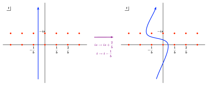
Figure 8: Shift of the integration contour.

To find some shift equations for the integral (C.1d), it is useful to rewrite it as

$$\sinh(\pi bs)\,{\cal C}_{3}^{(1)}={\pi\over 4}\int\limits_{-i\infty}^{i\infty}dt\,{\cot(\pi bt)-\cot[\pi b(is+t)]\over\sin\left[{\pi\over b}\left(\beta+i{s-s^{\prime}\over 2}+t\right)\right]\sin\left[{\pi\over b}\left({1\over b}-\beta+i{s-s^{\prime}\over 2}+t\right)\right]}.$$ (C.12)

Now let us consider, for instance, the shift $is\to is+2/b$. It has an effect only on the arguments of the sine functions in the denominator. However, the change of the arguments can be compensated by shifting the integration variable $t\to t-1/b$. One could think that this brings us back to the initial integral, but this is not precisely the case. The difference comes from the definition of the contour of integration described in section 2.2. Despite our shifts not being seen in the cotangent functions in the numerator, it is easy to see that they modify the integration contour in such a way that one pole of $\cot(\pi bt)$ passes the contour from the right to the left and one pole of $\cot[\pi b(is+t)]$ from the left to the right. We show this schematically in fig. 8. Therefore, in order to revert to the original integral, one has to add (subtract) the contribution of these poles. As a result, one arrives at the following equation satisfied by the integral (C.12)

$$\begin{split}&\left(e^{-{2i\over b}\partial_{s}}-1\right)\left[\sinh(\pi bs)\,{\cal C}_{3}^{(1)}\right]\\ &\qquad=\textstyle{\pi i\over 2b}\left({1\over\sin\left[{\pi\over b}\left(\beta+i{s-s^{\prime}\over 2}\right)\right]\sin\left[{\pi\over b}\left({1\over b}-\beta+i{s-s^{\prime}\over 2}\right)\right]}+{1\over\sin\left[{\pi\over b}\left({1\over b}-\beta+i{s+s^{\prime}\over 2}\right)\right]\sin\left[{\pi\over b}\left(\beta+i{s+s^{\prime}\over 2}\right)\right]}\right)\\ &\qquad=\,\scriptstyle{\pi i\over 2b\sin\left[{\pi\over b}\left(2\beta-{1\over b}\right)\right]}\left(\cot\left[{\pi\over b}\left({1\over b}-\beta+i{s-s^{\prime}\over 2}\right)\right]-\cot\left[{\pi\over b}\left(\beta+i{s-s^{\prime}\over 2}\right)\right]-\cot\left[{\pi\over b}\left(\beta+i{s+s^{\prime}\over 2}\right)\right]+\cot\left[{\pi\over b}\left({1\over b}-\beta+i{s+s^{\prime}\over 2}\right)\right]\right).\end{split}$$ (C.13)

The shift $is\to is+2b$ works in a slightly different way. It does not influence the denominator and changes only the argument of the second cotangent. Because of this, it is convenient to consider (C.12) as a sum of two integrals and shift the integration variable, $t\to t-2b$, only in the second one. Then again the resulting integrals differ from the initial ones only by the contours of integration which pick up additional poles coming from the sine functions in the denominator. Considerations similar to the previous ones then lead to the following equation

$$\left(e^{-{2ib}\partial_{s}}-1\right)\left[\sinh(\pi bs)\,{\cal C}_{3}^{(1)}\right]\\ =\,\scriptstyle{\pi ib\over 2\sin\left[{\pi\over b}\left(2\beta-{1\over b}\right)\right]}\left(\cot\left[\pi b\left(b-\beta+i{s-s^{\prime}\over 2}\right)\right]-\cot\left[\pi b\left(\beta+i{s-s^{\prime}\over 2}\right)\right]-\cot\left[\pi b\left(\beta+i{s+s^{\prime}\over 2}\right)\right]+\cot\left[\pi b\left(b-\beta+i{s+s^{\prime}\over 2}\right)\right]\right).$$ (C.14)

In the same way, one can find other difference equations which involve shifts of $s^{\prime}$ and $\beta$. It is easy to check that (C.13), (C.14), as well as these other equations are satisfied by the function given in (C.8). Thus, the study of shift equations yields the same result that we reach by summing residues. This completes the analysis of the first of the three ways to derive the two-point function.

C.2 The cases $B^{s_{3}s_{2}}_{\beta_{2}}=B^{ss}_{b}$ and $B^{s_{1}s_{3}}_{\beta_{3}}=B^{ss}_{b}$

Now we turn to the computation of the two-point function from the three-point correlator in the two remaining cases. The first one is obtained by taking $\beta_{2}=b$, $\beta_{1}=\beta_{3}=\beta$ and $s_{2}=s_{3}=s$, $s_{1}=s^{\prime}$, whereas the second case corresponds to the choice $\beta_{3}=b$, $\beta_{1}=\beta_{2}=\beta$ and $s_{1}=s_{3}=s$, $s_{2}=s^{\prime}$. However, one can show that the expressions for the three-point function arising after these substitutions are related by a simple change of variables

$$s\to-s,\qquad s^{\prime}\to-s^{\prime},\qquad t\to\beta+i{s-s^{\prime}\over 2}-Q-t,$$ (C.15)

where we also showed the change of the integration variable that is needed. Since the final result, which is expected to coincide with (C.11), is an even function of the boundary parameters, this fact ensures that the two possibilities we consider here will give the same two-point function. Therefore, we concentrate only on the second case, $\beta_{3}=b$.

With this choice of the parameters, the three-point function reduces to:

$$C(\beta,\beta,b|s,s^{\prime},s)=\left[\pi\mu\gamma(b^{2})b^{2-2b^{2}}\right]^{{1\over 2b^{2}}-{\beta\over b}}{\cal C}^{(3)}_{1}\,{\cal C}^{(3)}_{2}\,{\cal C}^{(3)}_{3},$$ (C.16a)

$${\cal C}^{(3)}_{1} ={\Gamma_{b}\left(b\right)\Gamma_{b}\left({2\over b}+b-2\beta\right)\Gamma_{b}\left({1\over b}+2b-2\beta\right)\Gamma_{b}\left({1\over b}\right)\over\Gamma_{b}\left({1\over b}+b\right)\Gamma_{b}^{2}\left({1\over b}+b-2\beta\right)\Gamma_{b}\left({1\over b}-b\right)}=\frac{b\,{\cal C}^{(1)}_{1}}{{\bf S}_{b}\left(2\beta-b\right)},$$ (C.16b)

$${\cal C}^{(3)}_{2} ={{\bf S}_{b}\left({1\over b}\right){\bf S}_{b}\left({1\over b}-i{s}\right)\over{\bf S}_{b}\left(\beta+i{s^{\prime}-s\over 2}\right){\bf S}_{b}\left(\beta-i{s^{\prime}+s\over 2}\right)},$$ (C.16c)

$${\cal C}^{(3)}_{3} =-4\pi i\int\limits_{-i\infty}^{i\infty}dt\,\textstyle{{\bf S}_{b}\left({1\over b}+b-\beta+i{s+s^{\prime}\over 2}+t\right){\bf S}_{b}\left({1\over b}+b-\beta-i{s-s^{\prime}\over 2}+t\right){\bf S}_{b}\left(\beta+i{s^{\prime}-s\over 2}+t\right){\bf S}_{b}\left({1\over b}+b-\beta+i{s^{\prime}-s\over 2}+t\right)\over{\bf S}_{b}\left({1\over b}+b+i{s^{\prime}}+t\right){\bf S}_{b}\left({1\over b}+b+t\right){\bf S}_{b}\left({2\over b}+b-\beta+i{s^{\prime}-s\over 2}+t\right){\bf S}_{b}\left({1\over b}+2b-\beta+i{s^{\prime}-s\over 2}+t\right)}$$

$$=-\pi i\int\limits_{-i\infty}^{i\infty}\textstyle{dt\over\sin\left[\pi b\left(b-\beta-i{s-s^{\prime}\over 2}+t\right)\right]\sin\left[{\pi\over b}\left({1\over b}-\beta-i{s-s^{\prime}\over 2}+t\right)\right]}{{\bf S}_{b}\left(\beta+i{s^{\prime}-s\over 2}+t\right){\bf S}_{b}\left({1\over b}+b-\beta+i{s+s^{\prime}\over 2}+t\right)\over{\bf S}_{b}\left({1\over b}+b+t\right){\bf S}_{b}\left({1\over b}+b+i{s^{\prime}}+t\right)}.$$ (C.16d)

By shifting the parameters in ${\cal C}^{(3)}_{3}$ in various ways, one can again find some shift equations satisfied by the integral (C.16d). Due to the symmetry of the integral under $b\to 1/b$, it is enough to find equations which use only shifts by multiples of $b$. Then the symmetry guarantees the existence of similar equations with $b$ replaced by $1/b$, and the final result must be symmetric as well. We find for instance the following three equations

$$\left[\frac{\sin\left[\pi b\left(\beta-i\frac{s-s^{\prime}}{2}\right)\right]e^{-2ib\partial_{s^{\prime}}}-\sin\left[\pi b\left(b+is^{\prime}\right)\right]e^{-ib(\partial_{s}+\partial_{s^{\prime}})}}{\sin\left[\pi b\left(\beta-b-i\frac{s+s^{\prime}}{2}\right)\right]}-1\right]\ {\cal C}_{3}^{(3)} =0,$$ (C.17a)

$$\left[\frac{\sin\left[\pi b\left(\beta-b-i\frac{s+s^{\prime}}{2}\right)\right]e^{-2ib\partial_{s^{\prime}}}-\sin\left[\pi b\left(b+is^{\prime}\right)\right]e^{\frac{b}{2}\partial_{\beta}-ib\partial_{s^{\prime}}}}{\sin\left[\pi b\left(\beta-i\frac{s-s^{\prime}}{2}\right)\right]}-1\right]\ {\cal C}_{3}^{(3)} =0,$$ (C.17b)

$$\textstyle\Bigg{[}\frac{\sin\left[\pi b\left(\beta-b-i\frac{s+s^{\prime}}{2}\right)\right]}{\sin\left[\pi b\left(b-2\beta+is\right)\right]}\left(e^{-\frac{b}{2}\partial_{\beta}-ib\partial_{s^{\prime}}}+\frac{\sin\left[\pi b\left(is-b\right)\right]}{\sin\left[\pi b\left(2\beta-b\right)\right]}\,e^{ib\left(\partial_{s}-\partial_{s^{\prime}}\right)}\right)-\frac{\sin\left[\pi b\left(\beta+i\frac{s+s^{\prime}}{2}\right)\right]}{\sin\left[\pi b\left(2\beta-b\right)\right]}\,e^{\frac{b}{2}\partial_{\beta}-ib\partial_{s^{\prime}}}-1\Bigg{]}{\cal C}_{3}^{(3)}\\ \textstyle=\frac{2\pi b\,\sin\left[\pi b\left(b-\beta+i\frac{s+s^{\prime}}{2}\right)\right]}{\sin\left[\pi b\left(\beta+i\frac{s+s^{\prime}}{2}\right)\right]\sin\left[\pi b\left(2\beta-b\right)\right]}\,\frac{{\bf S}_{b}\left(2\beta-b-\frac{1}{b}\right){\bf S}_{b}\left(is\right)}{{\bf S}_{b}\left(\beta+i{s+s^{\prime}\over 2}\right){\bf S}_{b}\left(\beta+i{s-s^{\prime}\over 2}\right)}.$$ (C.17c)

The origin of the non-homogeneous right hand side in the third equation can be again traced back to the shift of the integration contour. Both shift operators $e^{-\frac{b}{2}\partial_{\beta}-ib\partial_{s^{\prime}}}$ and $e^{ib\left(\partial_{s}-\partial_{s^{\prime}}\right)}$ transform the arguments of the sine functions in the integrand (C.16d) so that one has to pick the residues at the poles situated at $t=i\frac{s-s^{\prime}}{2}+\beta-2b$ and $t=i\frac{s-s^{\prime}}{2}+\beta-b-\frac{1}{b}$ in order to revert to the original contour of integration. The sum of the contributions of these four residues gives the right hand side of (C.17c).

One can show that the following expression for ${\cal C}_{3}^{(3)}$

$${\cal C}_{3}^{(3)}=-\frac{4i\,{\bf S}_{b}\left(2\beta-b-\frac{1}{b}\right){\bf S}_{b}\left(is\right)}{{\bf S}_{b}\left(\beta+i{s+s^{\prime}\over 2}\right){\bf S}_{b}\left(\beta+i{s-s^{\prime}\over 2}\right)}\ \frac{\partial}{\partial s}\log{{\bf S}_{b}\left({1\over b}+b-\beta+i{s-s^{\prime}\over 2}\right){\bf S}_{b}\left({1\over b}+b-\beta+i{s+s^{\prime}\over 2}\right)\over{\bf S}_{b}\left(\beta+i{s+s^{\prime}\over 2}\right){\bf S}_{b}\left(\beta+i{s-s^{\prime}\over 2}\right)}.$$ (C.18)

satisfies all of the above shift equations. When combined with (C.16b) and (C.16c), (C.18) reproduces precisely the expression (C.9) and thus leads to the same two-point function that was obtained in the first part of this appendix.

We conclude that all three possibilities to get the two-point function starting from the three-point correlator give the same result (2.24), which differs from the boundary reflection amplitude by a simple momentum dependent factor. This provides a non-trivial check of the cyclic symmetry of the representation (2.20) for the three-point function and gives strong evidences in favor of its correctness.

C.3 One-point functions

We can also derive the one-point function of the cosmological constant operator starting from the result (2.24). Putting $\beta=b$ and $s_{1}=s_{2}=s$, one obtains

$$d(b|s,s) = 2\left({1\over b}-b\right)\left[\pi\mu\gamma(b^{2})b^{2-2b^{2}}\right]^{{1-b^{2}\over 2b^{2}}}{\Gamma_{b}\left(b-{1\over b}\right)\over\Gamma_{b}\left({1\over b}-b\right)}\,{{\bf S}_{b}\left(is+{1\over b}\right)\over{\bf S}_{b}\left(is+b\right)}\,{{\bf S}_{b}\left({1\over b}\right)\over{\bf S}_{b}\left(b\right)}$$ (C.19)

$$= -{2\over b}\left[\pi\mu\gamma(b^{2})\right]^{{1-b^{2}\over 2b^{2}}}{\Gamma\left(2-{1\over b^{2}}\right)\over\Gamma\left(1-b^{2}\right)}\,{\sinh(\pi s/b)\over\sinh(\pi sb)}.$$

The first integral with respect to $-\mu_{{}_{B}}$ gives the boundary one-point function of $B_{b}^{ss}$ given in (2.25), which we denote by $W(s)$ since it corresponds to the resolvent in the matrix model formulation. The second integral gives the disk partition function with FZZT boundary conditions

$$Z(s)=-\left[\pi\mu\gamma(b^{2})\right]^{{1+b^{2}\over 2b^{2}}}{b^{2}\Gamma\left(2-{1\over b^{2}}\right)\Gamma\left(1-b^{2}\right)\over\pi^{2}}\left({\cosh\left(\left(b+{1\over b}\right)\pi s\right)\over b+{1\over b}}+{\cosh\left(\left(b-{1\over b}\right)\pi s\right)\over b-{1\over b}}\right).$$ (C.20)

As a last step one has to evaluate the derivative with respect to $-\mu$, keeping $\mu_{{}_{B}}$ constant. The result

$$-{\partial Z\over\partial\mu}={1\over\pi b}\left[\pi\mu\gamma(b^{2})\right]^{{1-b^{2}\over 2b^{2}}}\Gamma\left(b^{2}\right)\Gamma\left(1-\textstyle{1\over b^{2}}\right)\cosh\left(\left(b-\textstyle{1\over b}\right)\pi s\right)=U(b|s)$$ (C.21)

shows that the one-point function obtained from the boundary three-point function, with the normalization that we have chosen, precisely coincides with the same quantity derived from the bulk-boundary correlator. This justifies the inclusion of the factor $4\pi$ into the initial expression for the three-point function.

Appendix D Details on the boundary three-point function

D.1 Evaluating the integral

In this appendix we study the integral (5.39) appearing in the calculation of the three-point function for degenerate momenta of the matter part. For convenience we rewrite it here:

$$\begin{split}\mathcal{C}_{3}=&\,\frac{\pi i(-1)^{\sum n_{i}}}{4^{n_{1}}}\int\limits_{-i\infty}^{i\infty}dt\,\frac{{\bf S}_{b}\left(t+{n_{1}+1\over b}+i{\tau_{1}+\tau_{2}\over 2\pi b}\right)\,{\bf S}_{b}\left(t+{n_{1}+1\over b}-i{\tau_{1}-\tau_{2}\over 2\pi b}\right)}{{\bf S}_{b}\left(t+{n_{2}+1\over b}+i{\tau_{2}-\tau_{3}\over 2\pi b}\right)\,{\bf S}_{b}\left(t+b+{1\over b}\right)}\\ &\times\textstyle\left[\prod\limits_{k=n_{2}+1}^{n_{1}+n_{3}+1}\sin\left(\frac{\pi}{b}\left(t+i\frac{\tau_{2}-\tau_{3}}{2\pi b}+\frac{k}{b}\right)\right)\prod\limits_{k=-n_{2}}^{n_{1}-n_{3}}\sin\left(\frac{\pi}{b}\left(t+i\frac{\tau_{2}-\tau_{3}}{2\pi b}+\frac{k}{b}\right)\right)\right]^{-1}.\end{split}$$ (D.1)

First, following the method used in appendix C, we derive some shift equations satisfied by this integral. They can be obtained by applying various shift operators to the integrand and, if necessary, also by shifting the integration variable. As explained in detail in appendix C, one should take a special care of a possible change of the integration contour which can produce non-homogeneous contributions to the equations. In this way we find the following equations

$$\left[\frac{\sinh\left({\tau_{1}-\tau_{2}\over 2b^{2}}-{\pi in_{1}\over b^{2}}\right)\,e^{-2\pi i\partial_{\tau_{2}}}-\sinh\left({\tau_{2}\over b^{2}}-{\pi i\over b^{2}}\right)\,e^{-\pi i\left(\partial_{\tau_{1}}+\partial_{\tau_{2}}+\partial_{\tau_{3}}\right)}}{\sinh\left({\tau_{1}+\tau_{2}\over 2b^{2}}-{\pi i(n_{1}+1)\over b^{2}}\right)}-1\right]{\cal C}_{3} =0,$$ (D.2a)

$$\left[\frac{\sinh\left({\tau_{1}-\tau_{2}\over 2}+\pi ib^{2}\right)\,e^{-2\pi ib^{2}\partial_{\tau_{2}}}+(-1)^{n_{1}}\sinh\left(\tau_{2}-\pi ib^{2}\right)\,e^{-\pi ib^{2}\left(\partial_{\tau_{1}}+\partial_{\tau_{2}}+\partial_{\tau_{3}}\right)}}{\sinh{\tau_{1}+\tau_{2}\over 2}}-1\right]{\cal C}_{3} =0,$$ (D.2b)

$$\left[e^{-2\pi ib^{2}\partial_{\tau_{3}}}-1\right]{\cal C}_{3}=2\pi i\left(\sum\limits_{j=-n_{2}}^{n_{1}-n_{3}}\operatorname{Res}\limits_{t=t_{j0}}+\sum\limits_{j=n_{2}+1}^{n_{1}+n_{3}+1}\operatorname{Res}\limits_{t=t_{j1}}\right)\mathcal{I}(t),$$ (D.2c)

$$\left[\frac{\sinh\left({\tau_{1}-\tau_{2}\over 2}-\pi ib^{2}\right)}{\sinh{\tau_{1}+\tau_{2}\over 2}}\left(e^{-2\pi ib^{2}\partial_{\tau_{1}}}+\frac{\sinh(\tau_{1}-\pi ib^{2})}{\sinh(\tau_{2}-\pi ib^{2})}\,e^{-2\pi ib^{2}\partial_{\tau_{2}}}\right)-\frac{\sinh(\tau_{1}-\pi ib^{2})}{\sinh(\tau_{2}-\pi ib^{2})}+1\right]{\cal C}_{3}$$

$$\ \ =-2\pi i\,\frac{\sinh\left(\tau_{1}-\pi ib^{2}\right)}{\sinh{\tau_{1}+\tau_{2}\over 2}}\left(\sum\limits_{j=-n_{2}}^{n_{1}-n_{3}}\operatorname{Res}\limits_{t=t_{j0}}+\sum\limits_{j=n_{2}+1}^{n_{1}+n_{3}+1}\operatorname{Res}\limits_{t=t_{j1}}\right)\frac{\sin(\pi bt)\,\mathcal{I}(t)}{\sin\left[\pi b\left(t-i{\tau_{1}-\tau_{2}\over 2\pi b}-b\right)\right]},$$ (D.2d)

where $\mathcal{I}(t)$ denotes the integrand (together with the numerical prefactor) and $t_{jl}$ are its poles coming from the sine functions in the denominator

$$t_{jl}=-i\frac{\tau_{2}-\tau_{3}}{2\pi b}-\frac{j}{b}+lb.$$ (D.3)

The corresponding residues of $\mathcal{I}(t)$ were calculated in (5.41). In the last equation they appear multiplied by the factor $\frac{\sin(\pi bt_{jl})}{\sin\left[\pi b\left(t_{jl}-i{\tau_{1}-\tau_{2}\over 2\pi b}-b\right)\right]}$.

Then, by straightforward but tedious calculations, one can show that all equations are satisfied by the following function

$$\begin{split}\mathcal{C}_{3}&=2\pi b\ (-1)^{\sum n_{i}+1}4^{n_{2}+n_{3}}\,{\hat{\mu}}\,{{\bf S}_{b}\left(b-{n_{3}\over b}-i{\tau_{1}-\tau_{3}\over 2\pi b}\right){\bf S}_{b}\left(b-{n_{3}\over b}+i{\tau_{1}+\tau_{3}\over 2\pi b}\right)\over{\bf S}_{b}\left({n_{2}+1\over b}-i{\tau_{2}-\tau_{3}\over 2\pi b}\right){\bf S}_{b}\left({n_{2}+1\over b}+i{\tau_{2}+\tau_{3}\over 2\pi b}\right)}\\ &\qquad\qquad\times\Bigg{\{}\frac{1}{\hat{\mu}_{12}\hat{\mu}_{23}}\sum_{j=n_{2}+1}^{n_{1}+n_{3}+1}\frac{\mathcal{A}_{j}}{\prod\limits_{k=n_{2}+1\atop k\neq j}^{n_{1}+n_{3}+1}\sin\left(\frac{\pi}{b^{2}}\left(k-j\right)\right)\prod\limits_{k=-n_{2}}^{n_{1}-n_{3}}\sin\left(\frac{\pi}{b^{2}}\left(k-j\right)\right)}\\ &\qquad\qquad\quad+\frac{1}{\hat{\mu}_{12}\hat{\mu}_{13}}\sum_{j=-n_{2}}^{n_{1}-n_{3}}\frac{\mathcal{A}_{j}}{\prod\limits_{k=n_{2}+1}^{n_{1}+n_{3}+1}\sin\left(\frac{\pi}{b^{2}}\left(k-j\right)\right)\prod\limits_{k=-n_{2}\atop k\neq j}^{n_{1}-n_{3}}\sin\left(\frac{\pi}{b^{2}}\left(k-j\right)\right)}\Bigg{\}},\end{split}$$ (D.4)

where ${\cal A}_{j}$ is given in (5.44) or in (5.51). Since the ratio of ${\bf S}_{b}$ functions coincides with ${\cal C}_{2}^{-1}$ (cf. (5.36c)), this is precisely the result (5.46) which we obtained in the main text by closing the contour of integration in (D.1) in the right half plane and summing the residues of the integrand only at the poles which are due to the sine functions. This gives convincing evidence of the correctness of the use of these “effective integration rules”.

D.2 Explicit results for the three-point function

This subsection contains explicit expressions of the three-point function for various low values of momenta $n_{i}$. We consider all cases up to $\sum n_{i}\leq 4$ and satisfying the triangle inequality $|n_{2}-n_{3}|\leq n_{1}\leq n_{2}+n_{3}$. The results are expressed in terms of the one point functions $\hat{W}_{i}\equiv\hat{W}(\tau_{i})$. We will use the shorthand ${\hat{\mu}}_{i}={\hat{\mu}_{{}_{B}}}(\tau_{i})$, and we recall that the expression of the coefficients $a_{n}$ is given in (5.32).

$$\hat{C} (\beta_{0},\beta_{0},\beta_{0}|\tau_{1},\tau_{2},\tau_{3})=\frac{1}{{\hat{\mu}}_{12}\ {\hat{\mu}}_{23}\ {\hat{\mu}}_{31}}\left[{\hat{\mu}}_{1}(\hat{W}_{2}-\hat{W}_{3})+{\hat{\mu}}_{2}(\hat{W}_{3}-\hat{W}_{1})+{\hat{\mu}}_{3}(\hat{W}_{1}-\hat{W}_{2})\right]\,,$$ (D.5)

$$\hat{C} (\beta_{0},\beta_{1},\beta_{1}|\tau_{1},\tau_{2},\tau_{3})=\frac{a_{1}}{{\hat{\mu}}_{12}\ {\hat{\mu}}_{23}\ {\hat{\mu}}_{31}}$$

$$\times\Bigg{\{}\left[{\hat{\mu}}_{1}\left(\hat{W}_{2}^{3}-\hat{W}_{3}^{3}-\frac{\sin{\frac{3\pi}{b^{2}}}}{\sin{\frac{\pi}{b^{2}}}}\hat{W}_{2}\hat{W}_{3}(\hat{W}_{2}-\hat{W}_{3})-\frac{16b^{2}}{\pi^{2}}{\hat{\mu}}^{\frac{1}{b^{2}}}\cos^{2}{\textstyle\frac{\pi}{b^{2}}}(\hat{W}_{2}-\hat{W}_{3})\right)-(1\leftrightarrow 2)\right]$$ (D.6)

$$+{\hat{\mu}}_{3}\left(\hat{W}_{1}^{3}-\hat{W}_{2}^{3}+\frac{\sin{\frac{3\pi}{b^{2}}}}{\sin{\frac{\pi}{b^{2}}}}(\hat{W}_{3}^{2}(\hat{W}_{1}-\hat{W}_{2})-\hat{W}_{3}(\hat{W}_{1}^{2}-\hat{W}_{2}^{2}))-\frac{16b^{2}}{\pi^{2}}{\hat{\mu}}^{\frac{1}{b^{2}}}\cos^{2}{\textstyle\frac{\pi}{b^{2}}}(\hat{W}_{1}-\hat{W}_{2})\right)\Bigg{\}}$$

$$\hat{C} (\beta_{1},\beta_{1},\beta_{1}|\tau_{1},\tau_{2},\tau_{3})=\frac{a_{3/2}}{{\hat{\mu}}_{12}\ {\hat{\mu}}_{23}\ {\hat{\mu}}_{31}}\frac{2\cos{\textstyle\frac{2\pi}{b^{2}}}\ b^{2}\ \Gamma\left(\frac{2}{b^{2}}\right)^{2}}{\Gamma\left(\frac{1}{b^{2}}\right)\Gamma\left(\frac{4}{b^{2}}-1\right)}\Bigg{\{}{\hat{\mu}}_{1}\Bigg{(}\hat{W}_{2}^{4}-\hat{W}_{3}^{4}$$

$$-2\cos{\textstyle\frac{2\pi}{b^{2}}}(\hat{W}_{1}(\hat{W}_{2}^{3}-\hat{W}_{3}^{3})+\hat{W}_{2}\hat{W}_{3}(\hat{W}_{2}^{2}-\hat{W}_{3}^{2}))+2\cos{\textstyle\frac{2\pi}{b^{2}}}\ \frac{\sin{\frac{3\pi}{b^{2}}}}{\sin{\frac{\pi}{b^{2}}}}\hat{W}_{1}\hat{W}_{2}\hat{W}_{3}(\hat{W}_{2}-\hat{W}_{3})$$ (D.7)

$$-\frac{16b^{2}}{\pi^{2}}{\hat{\mu}}^{\frac{1}{b^{2}}}\cos^{2}{\textstyle\frac{\pi}{b^{2}}}\left(\hat{W}_{2}^{2}-\hat{W}_{3}^{2}-2\cos{\textstyle\frac{2\pi}{b^{2}}}\hat{W}_{1}(\hat{W}_{2}-\hat{W}_{3})\right)\Bigg{)}+\text{cyclic permutations}\Bigg{\}}$$

$$\hat{C} (\beta_{0},\beta_{2},\beta_{2}|\tau_{1},\tau_{2},\tau_{3})=\frac{a_{2}}{{\hat{\mu}}_{12}\ {\hat{\mu}}_{23}\ {\hat{\mu}}_{31}}$$

$$\times\Bigg{\{}\Bigg{[}{\hat{\mu}}_{1}\Bigg{(}\hat{W}_{2}^{5}-\hat{W}_{3}^{5}-\frac{\sin{\frac{5\pi}{b^{2}}}}{\sin{\frac{\pi}{b^{2}}}}\hat{W}_{2}\hat{W}_{3}(\hat{W}_{2}^{3}-\hat{W}_{3}^{3})+2\cos{\textstyle\frac{2\pi}{b^{2}}}\ \frac{\sin{\frac{5\pi}{b^{2}}}}{\sin{\frac{\pi}{b^{2}}}}\hat{W}_{2}^{2}\hat{W}_{3}^{2}(\hat{W}_{2}-\hat{W}_{3})$$

$$-\frac{16b^{2}}{\pi^{2}}{\hat{\mu}}^{\frac{1}{b^{2}}}\cos^{2}{\textstyle\frac{\pi}{b^{2}}}\left(\left(1+4\cos^{2}{\textstyle\frac{2\pi}{b^{2}}}\right)(\hat{W}_{2}^{3}-\hat{W}_{3}^{3})-\frac{\sin{\frac{3\pi}{b^{2}}}\sin{\frac{5\pi}{b^{2}}}}{\sin^{2}{\frac{\pi}{b^{2}}}}\hat{W}_{2}\hat{W}_{3}(\hat{W}_{2}-\hat{W}_{3})\right)$$

$$+\frac{1024b^{4}}{\pi^{4}}{\hat{\mu}}^{\frac{2}{b^{2}}}\cos^{4}{\textstyle\frac{\pi}{b^{2}}}\cos^{2}{\textstyle\frac{2\pi}{b^{2}}}(\hat{W}_{2}-\hat{W}_{3})\Bigg{)}-(1\leftrightarrow 2)\Bigg{]}+{\hat{\mu}}_{3}\Bigg{(}\hat{W}_{1}^{5}-\hat{W}_{2}^{5}$$ (D.8)

$$+\frac{\sin{\frac{5\pi}{b^{2}}}}{\sin{\frac{\pi}{b^{2}}}}(\hat{W}_{3}^{4}(\hat{W}_{1}-\hat{W}_{2})-\hat{W}_{3}(\hat{W}_{1}^{4}-\hat{W}_{2}^{4}))-2\cos{\textstyle\frac{2\pi}{b^{2}}}\ \frac{\sin{\frac{5\pi}{b^{2}}}}{\sin{\frac{\pi}{b^{2}}}}(\hat{W}_{3}^{3}(\hat{W}_{1}^{2}-\hat{W}_{2}^{2})-\hat{W}_{3}^{2}(\hat{W}_{1}^{3}-\hat{W}_{2}^{3}))$$

$$-\frac{16b^{2}}{\pi^{2}}{\hat{\mu}}^{\frac{1}{b^{2}}}\cos^{2}{\textstyle\frac{\pi}{b^{2}}}\ \Big{(}\left(1+4\cos^{2}{\textstyle\frac{2\pi}{b^{2}}}\right)(\hat{W}_{1}^{3}-\hat{W}_{2}^{3})+\frac{\sin{\frac{3\pi}{b^{2}}}\sin{\frac{5\pi}{b^{2}}}}{\sin^{2}{\frac{\pi}{b^{2}}}}(\hat{W}_{3}^{2}(\hat{W}_{1}-\hat{W}_{2})-\hat{W}_{3}(\hat{W}_{1}^{2}-\hat{W}_{2}^{2}))\Big{)}$$

$$+\frac{1024b^{4}}{\pi^{4}}{\hat{\mu}}^{\frac{2}{b^{2}}}\cos^{4}{\textstyle\frac{\pi}{b^{2}}}\cos^{2}{\textstyle\frac{2\pi}{b^{2}}}(\hat{W}_{1}-\hat{W}_{2})\Bigg{)}\Bigg{\}}$$

$$\hat{C} (\beta_{1},\beta_{1},\beta_{2}|\tau_{1},\tau_{2},\tau_{3})=\frac{a_{2}}{{\hat{\mu}}_{12}\ {\hat{\mu}}_{23}\ {\hat{\mu}}_{31}}\Bigg{\{}\Bigg{[}{\hat{\mu}}_{3}\Bigg{(}\hat{W}_{1}^{5}-2\cos{\textstyle\frac{2\pi}{b^{2}}}\ \frac{\sin{\frac{3\pi}{b^{2}}}}{\sin{\frac{\pi}{b^{2}}}}\hat{W}_{2}^{5}+\frac{\sin{\frac{3\pi}{b^{2}}}\sin{\frac{5\pi}{b^{2}}}}{\sin^{2}{\frac{\pi}{b^{2}}}}(\hat{W}_{2}^{4}(\hat{W}_{3}+\hat{W}_{1}))$$

$$-\frac{\sin{\frac{5\pi}{b^{2}}}}{\sin{\frac{\pi}{b^{2}}}}\hat{W}_{3}\hat{W}_{1}^{4}-2\cos{\textstyle\frac{2\pi}{b^{2}}}\ \frac{\sin{\frac{5\pi}{b^{2}}}}{\sin{\frac{\pi}{b^{2}}}}\left(\hat{W}_{2}^{3}\left(\hat{W}_{3}^{2}+\hat{W}_{1}^{2}+4\cos^{2}{\textstyle\frac{\pi}{b^{2}}}\hat{W}_{3}\hat{W}_{1}\right)-\hat{W}_{3}^{2}\hat{W}_{1}^{3}\right)$$

$$-2\cos{\textstyle\frac{2\pi}{b^{2}}}\ \frac{\sin{\frac{3\pi}{b^{2}}}\sin{\frac{5\pi}{b^{2}}}}{\sin^{2}{\frac{\pi}{b^{2}}}}\hat{W}_{3}\hat{W}_{1}\hat{W}_{2}(\hat{W}_{3}\hat{W}_{1}-\hat{W}_{1}\hat{W}_{2}-\hat{W}_{2}\hat{W}_{3})$$

$$-\frac{16b^{2}}{\pi^{2}}{\hat{\mu}}^{\frac{1}{b^{2}}}\cos^{2}{\textstyle\frac{\pi}{b^{2}}}\Big{(}\left(1+4\cos^{2}{\textstyle\frac{2\pi}{b^{2}}}\right)\hat{W}_{1}^{3}-2\cos{\textstyle\frac{2\pi}{b^{2}}}\left(1+4\cos{\textstyle\frac{2\pi}{b^{2}}}\right)\hat{W}_{2}^{3}-\frac{\sin{\frac{5\pi}{b^{2}}}}{\sin{\frac{\pi}{b^{2}}}}\hat{W}_{3}\hat{W}_{1}^{2}$$

$$+\frac{\sin{\frac{3\pi}{b^{2}}}\sin{\frac{5\pi}{b^{2}}}}{\sin^{2}{\frac{\pi}{b^{2}}}}\hat{W}_{2}^{2}(\hat{W}_{3}+\hat{W}_{1})-2\cos{\textstyle\frac{2\pi}{b^{2}}}\ \frac{\sin{\frac{5\pi}{b^{2}}}}{\sin{\frac{\pi}{b^{2}}}}(\hat{W}_{2}(\hat{W}_{3}^{2}+\hat{W}_{1}^{2}+\hat{W}_{3}\hat{W}_{1})-\hat{W}_{3}^{2}\hat{W}_{1})\Big{)}$$

$$+\frac{1024b^{4}}{\pi^{4}}{\hat{\mu}}^{\frac{2}{b^{2}}}\cos^{4}{\textstyle\frac{\pi}{b^{2}}}\cos^{2}{\textstyle\frac{2\pi}{b^{2}}}(\hat{W}_{1}-\hat{W}_{2})\Bigg{)}-(3\leftrightarrow 1)\Bigg{]}$$ (D.9)

$$+{\hat{\mu}}_{2}\Bigg{(}\hat{W}_{3}^{5}-\hat{W}_{1}^{5}-\frac{\sin{\frac{5\pi}{b^{2}}}}{\sin{\frac{\pi}{b^{2}}}}\hat{W}_{3}\hat{W}_{1}(\hat{W}_{3}^{3}-\hat{W}_{1}^{3})+2\cos{\textstyle\frac{2\pi}{b^{2}}}\ \frac{\sin{\frac{5\pi}{b^{2}}}}{\sin{\frac{\pi}{b^{2}}}}\hat{W}_{3}^{2}\hat{W}_{1}^{2}(\hat{W}_{3}-\hat{W}_{1})$$

$$-\frac{16b^{2}}{\pi^{2}}{\hat{\mu}}^{\frac{1}{b^{2}}}\cos^{2}{\textstyle\frac{\pi}{b^{2}}}\left(\left(1+4\cos^{2}{\textstyle\frac{2\pi}{b^{2}}}\right)(\hat{W}_{3}^{3}-\hat{W}_{1}^{3})-\frac{\sin{\frac{3\pi}{b^{2}}}\sin{\frac{5\pi}{b^{2}}}}{\sin^{2}{\frac{\pi}{b^{2}}}}\hat{W}_{3}\hat{W}_{1}(\hat{W}_{3}-\hat{W}_{1})\right)$$

$$+\frac{1024b^{4}}{\pi^{4}}{\hat{\mu}}^{\frac{2}{b^{2}}}\cos^{4}{\textstyle\frac{\pi}{b^{2}}}\cos^{2}{\textstyle\frac{2\pi}{b^{2}}}(\hat{W}_{3}-\hat{W}_{1})\Bigg{)}\Bigg{\}}$$

All of the above results satisfy the required properties of being real and cyclically symmetric in the momenta. In particular, cyclic symmetry is evident for $(n_{1},n_{2},n_{3})=(0,0,0)$ and $(1,1,1)$, while we checked it for the other cases explicitly (notice that in order to check the symmetry one also has to interchange the chiralities of the operators and thus to take into account the fact that different renormalization factors must be used).

D.3 $d$ from $C$ once again

Our purpose here is to do a consistency check, namely to verify that the $c=1$ limit of the three-point function produces the same two-point function which was derived in section 5.4. In fact, we can do better and check that one function follows from the other before taking the limit, but after the momenta degenerate in the matter sector were substituted and all special functions and integrals were eliminated. Then the agreement of the limiting expressions trivially follows.

In other words, we are going to show that if one takes the expression (5.52), puts $(n_{1},n_{2},n_{3})=(0,n,n)$, $(\tau_{1},\tau_{2},\tau_{3})=(\tau,\tau,\tau^{\prime})$ and integrates with respect to $-{\hat{\mu}_{{}_{B}}}(\tau)$, one obtains the result (5.31). Of course, one can choose two other possibilities to get the two-point correlator similar to the ones in appendix C.2. However, they require more complicated calculations, and we proceed here only with the first choice.

First, one can show that, after setting $n_{1}=0$, $n_{2}=n_{3}=n$, (5.52) becomes

$$\hat{C}(b,\beta_{n},\beta_{n}|\tau_{1},\tau_{2},\tau_{3})=-a_{n}\Bigg{\{}\frac{\scriptstyle\prod\limits_{k=-n}^{n}\left(\hat{W}(\tau_{2})-\hat{W}(\tau_{3}-2\pi ik)\right)}{\hat{\mu}_{12}\,\hat{\mu}_{23}}-\frac{\scriptstyle\prod\limits_{k=-n}^{n}\left(\hat{W}(\tau_{1})-\hat{W}(\tau_{3}-2\pi ik)\right)}{\hat{\mu}_{12}\,\hat{\mu}_{13}}\Bigg{\}},$$ (D.10)

where the coefficient $a_{n}$ is defined in (5.32). Then, taking the limit $\tau_{1}=\tau_{2}=\tau$, $\tau_{3}=\tau^{\prime}$, one obtains

$$\hat{C}(b,\beta_{n},\beta_{n}|\tau,\tau,\tau^{\prime})=-{a_{n}\over\hat{\mu}_{\tau\tau^{\prime}}}\left\{\frac{\scriptstyle\prod\limits_{k=-n}^{n}\left(\hat{W}(\tau)-\hat{W}(\tau^{\prime}-2\pi ik)\right)}{\hat{\mu}_{\tau\tau^{\prime}}}-\frac{{\partial_{\tau}}\scriptstyle\prod\limits_{k=-n}^{n}\left(\hat{W}(\tau)-\hat{W}(\tau^{\prime}-2\pi ik)\right)}{{\partial_{\tau}}\hat{\mu}_{\tau\tau^{\prime}}}\right\}.$$ (D.11)

The integral is easily evaluated producing

$$-\int d{\hat{\mu}_{{}_{B}}}(\tau)\,\hat{C}(b,\beta_{n},\beta_{n}|\tau,\tau,\tau^{\prime})=-{a_{n}\over\hat{\mu}_{\tau\tau^{\prime}}}\prod\limits_{k=-n}^{n}\left(\hat{W}(\tau)-\hat{W}(\tau^{\prime}-2\pi ik)\right).$$ (D.12)

This result coincides with the two-point function $\hat{d}(\beta_{n}|\tau,\tau^{\prime})$ from (5.31). This constitutes a check of the correctness of our intermediate calculations in the derivation of the three-point function.

References

- [1] I. R. Klebanov, “String theory in two-dimensions,” hep-th/9108019.
- [2] P. H. Ginsparg and G. W. Moore, “Lectures on 2-D gravity and 2-D string theory,” hep-th/9304011.
- [3] E. J. Martinec, “Matrix models and 2D string theory,” hep-th/0410136.
- [4] J. McGreevy and H. Verlinde, “Strings from tachyons: The matrix reloaded,” JHEP 12 (2003) 054, hep-th/0304224.
- [5] E. J. Martinec, “The annular report on non-critical string theory,” hep-th/0305148.
- [6] I. R. Klebanov, J. Maldacena, and N. Seiberg, “D-brane decay in two-dimensional string theory,” JHEP 07 (2003) 045, hep-th/0305159.
- [7] J. McGreevy, J. Teschner, and H. Verlinde, “Classical and quantum D-branes in 2D string theory,” JHEP 01 (2004) 039, hep-th/0305194.
- [8] S. Y. Alexandrov, V. A. Kazakov, and D. Kutasov, “Non-perturbative effects in matrix models and D-branes,” JHEP 09 (2003) 057, hep-th/0306177.
- [9] M. R. Douglas et al., “A new hat for the matrix model,” hep-th/0307195.
- [10] M. Gutperle and P. Kraus, “D-brane dynamics in the matrix model,” Phys. Rev. D69 (2004) 066005, hep-th/0308047.
- [11] J. Teschner, “On boundary perturbations in Liouville theory and brane dynamics in noncritical string theories,” JHEP 04 (2004) 023, hep-th/0308140.
- [12] S. Alexandrov, “ ZZ branes and the matrix model,” Phys. Lett. B604 (2004) 115–122, hep-th/0310135.
- [13] J. de Boer, A. Sinkovics, E. Verlinde, and J.-T. Yee, “String interactions in matrix model,” JHEP 03 (2004) 023, hep-th/0312135.
- [14] D. Gaiotto and L. Rastelli, “A paradigm of open/closed duality: Liouville D-branes and the Kontsevich model,” hep-th/0312196.
- [15] V. A. Kazakov and I. K. Kostov, “Instantons in non-critical strings from the two-matrix model,” hep-th/0403152.
- [16] M. Hanada et al., “Loops versus matrices: The nonperturbative aspects of noncritical string,” Prog. Theor. Phys. 112 (2004) 131–181, hep-th/0405076.
- [17] D. Kutasov, K. Okuyama, J.-w. Park, N. Seiberg, and D. Shih, “Annulus amplitudes and ZZ branes in minimal string theory,” JHEP 08 (2004) 026, hep-th/0406030.
- [18] J. Ambjørn, S. Arianos, J. A. Gesser, and S. Kawamoto, “The geometry of ZZ-branes,” Phys. Lett. B599 (2004) 306–312, hep-th/0406108.
- [19] A. Sato and A. Tsuchiya, “ZZ brane amplitudes from matrix models,” JHEP 02 (2005) 032, hep-th/0412201.
- [20] S. Y. Alexandrov and I. K. Kostov, “Time-dependent backgrounds of 2D string theory: Non- perturbative effects,” JHEP 02 (2005) 023, hep-th/0412223.
- [21] R. de Mello Koch, A. Jevicki, and J. P. Rodrigues, “Instantons in CSFT,” hep-th/0412319.
- [22] T. Takayanagi and S. Terashima, “ matrix model from string field theory,” hep-th/0503184.
- [23] J. Teschner, “On Tachyon condensation and open-closed duality in the string theory,” hep-th/0504043.
- [24] V. Fateev, A. B. Zamolodchikov, and A. B. Zamolodchikov, “Boundary Liouville field theory. I: Boundary state and boundary two-point function,” hep-th/0001012.
- [25] J. Teschner, “Remarks on Liouville theory with boundary,” hep-th/0009138.
- [26] A. B. Zamolodchikov and A. B. Zamolodchikov, “Liouville field theory on a pseudosphere,” hep-th/0101152.
- [27] K. Hosomichi, “Bulk-boundary propagator in Liouville theory on a disc,” JHEP 11 (2001) 044, hep-th/0108093.
- [28] B. Ponsot and J. Teschner, “Boundary Liouville field theory: Boundary three point function,” Nucl. Phys. B622 (2002) 309–327, hep-th/0110244.
- [29] B. Ponsot, “Liouville theory on the pseudosphere: Bulk-boundary structure constant,” Phys. Lett. B588 (2004) 105–110, hep-th/0309211.
- [30] Y. Nakayama, “Liouville field theory: A decade after the revolution,” Int. J. Mod. Phys. A19 (2004) 2771–2930, hep-th/0402009.
- [31] I. Runkel and G. M. T. Watts, “A non-rational CFT with as a limit of minimal models,” JHEP 09 (2001) 006, hep-th/0107118.
- [32] D. Ghoshal, S. Mukhi, and S. Murthy, “Liouville D-branes in two-dimensional strings and open string field theory,” JHEP 11 (2004) 027, hep-th/0406106.
- [33] N. Seiberg and D. Shih, “Branes, rings and matrix models in minimal (super)string theory,” JHEP 02 (2004) 021, hep-th/0312170.
- [34] C. Imbimbo and S. Mukhi, “The Topological matrix model of string,” Nucl. Phys. B449 (1995) 553–568, hep-th/9505127.
- [35] D. Ghoshal and C. Vafa, “ string as the topological theory of the conifold,” Nucl. Phys. B453 (1995) 121–128, hep-th/9506122.
- [36] R. Dijkgraaf and C. Vafa, “ supersymmetry, deconstruction, and bosonic gauge theories,” hep-th/0302011.
- [37] S. Mukhi, “Topological matrix models, Liouville matrix model and string theory,” hep-th/0310287.
- [38] M. Aganagic, R. Dijkgraaf, A. Klemm, M. Marino, and C. Vafa, “Topological strings and integrable hierarchies,” hep-th/0312085.
- [39] I. K. Kostov, B. Ponsot, and D. Serban, “Boundary Liouville theory and 2D quantum gravity,” Nucl. Phys. B683 (2004) 309–362, hep-th/0307189.
- [40] H. Dorn and H. J. Otto, “Two and three point functions in Liouville theory,” Nucl. Phys. B429 (1994) 375–388, hep-th/9403141.
- [41] A. B. Zamolodchikov and A. B. Zamolodchikov, “Structure constants and conformal bootstrap in Liouville field theory,” Nucl. Phys. B477 (1996) 577–605, hep-th/9506136.
- [42] O. Aharony, B. Fiol, D. Kutasov, and D. A. Sahakyan, “Little string theory and heterotic/type II duality,” Nucl. Phys. B679 (2004) 3–65, hep-th/0310197.
- [43] I. K. Kostov, “Boundary ground ring in 2D string theory,” Nucl. Phys. B689 (2004) 3–36, hep-th/0312301.
- [44] N. Seiberg, “Notes on quantum Liouville theory and quantum gravity,” Prog. Theor. Phys. Suppl. 102 (1990) 319–349.
- [45] S. Alexandrov, “D-branes and complex curves in string theory,” JHEP 05 (2004) 025, hep-th/0403116.
- [46] I. K. Kostov and V. B. Petkova, “Bulk correlation functions in 2D quantum gravity,” hep-th/0505078.
- [47] G. W. Moore, N. Seiberg, and M. Staudacher, “From loops to states in 2-D quantum gravity,” Nucl. Phys. B362 (1991) 665–709.
- [48] G. W. Moore and N. Seiberg, “From loops to fields in 2-D quantum gravity,” Int. J. Mod. Phys. A7 (1992) 2601–2634.
- [49] I. K. Kostov, “Strings with discrete target space,” Nucl. Phys. B376 (1992) 539–598, hep-th/9112059.
- [50] I. K. Kostov, “Gauge invariant matrix model for the A-D-E closed strings,” Phys. Lett. B297 (1992) 74–81, hep-th/9208053.
- [51] I. K. Kostov, “The ADE face models on a fluctuating planar lattice,” Nucl. Phys. B326 (1989) 583.
- [52] V. A. Kazakov and I. K. Kostov, “Loop gas model for open strings,” Nucl. Phys. B386 (1992) 520–557, hep-th/9205059.
- [53] I. K. Kostov, “Boundary correlators in 2D quantum gravity: Liouville versus discrete approach,” Nucl. Phys. B658 (2003) 397–416, hep-th/0212194.
- [54] R. Dijkgraaf, G. W. Moore, and M. R. Plesser, “The Partition function of 2D string theory,” Nucl. Phys. B394 (1993) 356–382, hep-th/9208031.
- [55] S. Y. Alexandrov, V. A. Kazakov, and I. K. Kostov, “Time-dependent backgrounds of 2D string theory,” Nucl. Phys. B640 (2002) 119–144, hep-th/0205079.
- [56] S. Alexandrov, “Matrix quantum mechanics and two-dimensional string theory in non-trivial backgrounds,” hep-th/0311273.