hep-th/0504194

Lectures on Twistor Strings
and Perturbative Yang-Mills Theory

Freddy Cachazo and Peter Svrček

Institute for Advanced Study, Princeton, NJ 08540, USA

Abstract

Recently, Witten proposed a topological string theory in twistor space that is dual to a weakly coupled gauge theory. In this lectures we will discuss aspects of the twistor string theory. Along the way we will learn new things about Yang-Mills scattering amplitudes. The string theory sheds light on Yang-Mills perturbation theory and leads to new methods for computing Yang-Mills scattering amplitudes.

April, 2005

1 Introduction

The idea that a gauge theory should be dual to a string theory goes back to ’t Hooft [51]. ’t Hooft considered $U(N)$ gauge theory in the large $N$ limit while keeping $\lambda=g_{YM}^{2}N$ fixed. He observed that the perturbative expansion of Yang-Mills can be reorganized in terms of Riemann surfaces, which he interpreted as an evidence for a hypothetical dual string theory with string coupling $g_{s}\sim 1/N.$

In 1997, Maldacena proposed a concrete example of this duality [60]. He considered the maximally supersymmetric Yang-Mills theory and conjectured that it is dual to type IIB string theory on $AdS_{5}\times S^{5}.$ This duality led to many new insights from string theory about gauge theories and vice versa. At the moment, we have control over the duality only for strongly coupled gauge theory. This corresponds to the limit of large radius of $AdS_{5}\times S^{5}$ in which the string theory is well described by supergravity. However, QCD is asymptotically free, so we would also like to have a string theory description of a weakly coupled gauge theory.

In weakly coupled field theories, the natural object to study is the perturbative $S$ matrix. The perturbative expansion of the $S$ matrix is conventionally computed using Feynman rules. Starting from early studies of de Witt [44], it was observed that scattering amplitudes show simplicity that is not apparent from the Feynman rules. For example, the maximally helicity violating (MHV) amplitudes can be expressed as simple holomorphic functions.

Recently, Witten proposed a string theory that is dual to a weakly coupled ${\cal N}=4$ gauge theory [76]. The perturbative expansion of the gauge theory is related to D-instanton expansion of the string theory. The string theory in question is the topological open string B-model on a Calabi-Yau supermanifold ${CP}^{3|4},$ which is a supersymmetric generalization of Penrose’s twistor space.

At tree level, evaluating the instanton contribution has led to new insights about scattering amplitudes. ‘Disconnected’ instantons give the MHV diagram construction of amplitudes in terms of Feynman diagrams with vertices that are suitable off-shell continuations of the MHV amplitudes [35]. The ‘connected’ instanton contributions express the amplitudes as integrals over the moduli space of holomorphic curves in twistor space [71]. Surprisingly, the MHV diagram construction and the connected instanton integral can be related via localization on the moduli space [43].

Despite the successes of the twistor string theory at tree level, there are still many open questions. The most pressing issue is perhaps the closed strings that give ${\cal N}=4$ conformal supergravity [16]. At tree level, it is possible to recover the Yang-Mills scattering amplitudes by extracting the single-trace amplitudes. At loop level, the single trace gluon scattering amplitudes receive contributions from internal supergravity states, so it would be difficult to extract the Yang-Mills contribution to the gluon scattering amplitudes. Since, ${\cal N}=4$ Yang-Mills theory is consistent without conformal supergravity, it is likely that there exists a version of the twistor string theory that is dual to pure Yang-Mills theory. Indeed, the MHV diagram construction that at tree level has been derived from twistor string theory seems to compute loop amplitudes as well [27].

The study of twistor structure of scattering amplitudes has inspired new developments in perturbative Yang-Mills theory itself. At tree level, this has led to recursion relations for on-shell amplitudes [30]. At one loop, unitarity techniques [24, 23] have been used to find new ways of computing ${\cal N}=4$ [29] and ${\cal N}=1$ [33] Yang-Mills amplitudes.

In these lectures we will discuss aspects of twistor string theory. Along the way we will learn lessons about Yang-Mills scattering amplitudes. The string theory sheds light on Yang-Mills perturbation theory and leads to new methods for computing Yang-Mills scattering amplitudes. In the last section, we will describe further developments in perturbative Yang-Mills.

2 Helicity Amplitudes

2.1 Spinors

Recall that the complexified Lorentz group is locally isomorphic to

$$SO(3,1,{C})\cong Sl(2,{C})\times Sl(2,{C}),$$ (1)

hence the finite dimensional representations are classified as $(p,q)$ where $p$ and $q$ are integer or half-integer. The negative and positive chirality spinors transform in the representations $(1/2,0)$ and $(0,1/2)$ respectively. We write generically $\lambda_{a},a=1,2$ for a spinor transforming as $(1/2,0)$ and $\tilde{\lambda}_{\dot{a}},\dot{a}=1,2$ for a spinor transforming as $(0,1/2).$

The spinor indices of type $(1/2,0)$ are raised and lowered using the antisymmetric tensors $\epsilon_{ab}$ and $\epsilon^{ab}$ obeying $\epsilon_{12}=1$ and $\epsilon^{ac}\epsilon_{cb}=\delta^{a}{}_{b}$

$$\lambda^{a}=\epsilon^{ab}\lambda_{b}\qquad\lambda_{a}=\epsilon_{ab}\lambda^{b}.$$ (2)

Given two spinors $\lambda$ and $\lambda^{\prime},$ both of negative chirality, we can form the Lorentz invariant product

$$\langle{\lambda,\lambda^{\prime}}\rangle=\epsilon_{ab}\lambda^{a}\lambda^{\prime}{}^{b}.$$ (3)

It follows that $\langle{\lambda,\lambda^{\prime}}\rangle=-\langle{\lambda^{\prime},\lambda}\rangle$, so the product is antisymmetric in its two variables. In particular, $\langle{\lambda,\lambda^{\prime}}\rangle=0$ implies that $\lambda$ equals $\lambda^{\prime}$ up to a scaling $\lambda^{a}=c\lambda^{\prime a}.$

Similarly, we lower and raise the indices of positive chirality spinors with the antisymmetric tensor $\epsilon_{\dot{a}\dot{b}}$ and its inverse $\epsilon^{\dot{a}\dot{b}}.$ For two spinors $\tilde{\lambda}$ and $\tilde{\lambda}^{\prime},$ both of positive chirality we define the antisymmetric product

$$[\tilde{\lambda},\tilde{\lambda}^{\prime}]=-[\tilde{\lambda}^{\prime},\tilde{\lambda}]=\epsilon_{\dot{a}\dot{b}}\tilde{\lambda}^{\dot{a}}\tilde{\lambda}^{\prime\dot{b}}.$$ (4)

The vector representation of $SO(3,1,{C})$ is the $(1/2,1/2)$ representation. Thus a momentum vector $p_{\mu},\mu=0,\dots,3$ can be represented as a bi-spinor $p_{a\dot{a}}$ with one spinor index $a$ and $\dot{a}$ of each chirality. The explicit mapping from $p_{\mu}$ to $p_{a\dot{a}}$ can be made using the chiral part of the Dirac matrices. In signature $+---,$ one can take the Dirac matrices to be

$$\gamma^{\mu}=\begin{pmatrix}0&\sigma^{\mu}\cr\overline{\sigma}^{\mu}&0\end{pmatrix},$$ (5)

where $\sigma^{\mu}=(1,\vec{\sigma}),\overline{\sigma}^{\mu}=(1,-\vec{\sigma})$ with $\vec{\sigma}$ being the $2\times 2$ Pauli matrices. For any vector, the relation between $p_{\mu},$ and $p_{a\dot{a}}$ is

$$p_{a\dot{a}}=p_{\mu}\sigma^{\mu}_{a\dot{a}}=p_{0}+\vec{\sigma}\cdot\vec{p}.$$ (6)

It follows that,

$$p_{\mu}p^{\mu}=\det(p_{a\dot{a}}).$$ (7)

Hence, $p_{\mu}$ is lightlike if the corresponding determinant is zero. This is equivalent to the rank of the $2\times 2$ matrix $p_{a\dot{a}}$ being less than or equal to one. So $p^{\mu}$ is lightlike precisely, when it can be written as a product

$$p_{a\dot{a}}=\lambda_{a}\tilde{\lambda}_{\dot{a}}$$ (8)

for some spinors $\lambda_{a}$ and $\tilde{\lambda}_{\dot{a}}.$ For a given null vector $p,$ the spinors $\lambda$ and $\tilde{\lambda}$ are unique up to a scaling

$$(\lambda,\tilde{\lambda})\rightarrow(t\lambda,t^{-1}\tilde{\lambda})\qquad t\in{C}^{\ast}.$$ (9)

There is no continuous way to pick $\lambda$ as a function $p.$ In Minkowski signature, the $\lambda$’s form the Hopf line bundle over the sphere $S^{2}$ of directions of the lightlike vector $p.$

For complex momenta, the spinors $\lambda^{a}$ and $\tilde{\lambda}^{\dot{a}}$ are independent complex variables, each of which parameterizes a copy of ${CP}^{1}.$ Hence, the complex lightcone $p_{\mu}p^{\mu}=0$ is a complex cone over the connected manifold ${CP}^{1}\times{CP}^{1}.$

For real null momenta in Minkowski signature $+---$, we can fix the scaling up to a $Z_{2}$ by requiring $\lambda^{a}$ and $\tilde{\lambda}^{\dot{a}}$ to be complex conjugates

$$\overline{\lambda}^{\dot{a}}=\pm\tilde{\lambda}^{\dot{a}}.$$ (10)

Hence, the negative chirality spinors $\lambda$ are conventionally called ‘holomorphic’ and the positive chirality spinor ‘anti-holomorphic.’ In (10) the $+$ sign is for a future pointing null vector $p^{\mu},$ and $-$ is for a past pointing $p^{\mu}.$

One can also consider other signatures. For example in the signature $++--,$ the spinors $\lambda$ and $\tilde{\lambda}$ are real and independent. Indeed, with signature $++--,$ the Lorentz group is $SO(2,2),$ which is locally isomorphic to $Sl(2,{R})\times Sl(2,{R}).$ Hence, the spinor representations are real.

Let us remark, that if $p$ and $p^{\prime}$ are two lightlike vectors given by $p_{a\dot{a}}=\lambda_{a}\tilde{\lambda}_{\dot{a}}$ and $p^{\prime}_{a\dot{a}}=\lambda^{\prime}_{a}\tilde{\lambda}^{\prime}_{\dot{a}}$ then their scalar product can be expressed as

$$2p\cdot p^{\prime}=\langle{\lambda,\lambda^{\prime}}\rangle[\tilde{\lambda},\tilde{\lambda}^{\prime}].$$ (11)

Given $p,$ the additional physical information in $\lambda$ is equivalent to a choice of wavefunction of a helicity $-1/2$ massless particle with momentum $p.$ To see this, we write the chiral Dirac equation for a negative chirality spinor $\psi^{a}$

$$0=i\sigma^{\mu}_{a\dot{a}}\partial_{\mu}\psi^{a}.$$ (12)

A plane wave $\psi^{a}=\rho^{a}\exp(ip\cdot x)$ satisfies this equation if and only if $p_{a\dot{a}}\rho^{a}=0.$ Writing $p_{a\dot{a}}=\lambda_{a}\tilde{\lambda}_{\dot{a}},$ we get $\lambda_{a}\rho^{a}=0,$ that is $\rho^{a}=c\cdot\lambda^{a}$ for a constant $c.$ Hence the negative helicity fermion has wavefunction

$$\psi^{a}=c\lambda^{a}\exp(ix_{a\dot{a}}\lambda^{a}\tilde{\lambda}^{\dot{a}}).$$ (13)

Similarly, $\tilde{\lambda}$ defines a wavefunction for a helicity $+1/2$ fermion $\psi^{\dot{a}}=c\tilde{\lambda}^{\dot{a}}\exp(ix_{a\dot{a}}\lambda^{a}\tilde{\lambda}^{\dot{a}}).$

There is an analogous description of wavefunctions of massless particles of helicity $\pm 1.$ Usually, we describe massless gluons with their momentum vector $p^{\mu}$ and polarization vector $\epsilon^{\mu}.$ The polarization vector obeys the constraint

$$p_{\mu}\ \epsilon^{\mu}=0$$ (14)

that represents the decoupling of longitudinal modes and it is subject to the gauge invariance

$$\epsilon^{\mu}\rightarrow\epsilon^{\mu}+wp^{\mu},$$ (15)

for any constant $w.$ Suppose that instead of being given only a lightlike vector $p_{a\dot{a}}$, one is also given a decomposition $p_{a\dot{a}}=\lambda_{a}\tilde{\lambda}_{\dot{a}}.$ Then we have enough information to determine the polarization vector up to a gauge transformation once the helicity is specified. For a positive helicity gluon, we take

$$\epsilon_{a\dot{a}}^{+}=\frac{\mu_{a}\tilde{\lambda}_{\dot{a}}}{\langle{\mu,\lambda}\rangle},$$ (16)

where $\mu$ is any negative chirality spinor that is not a multiple of $\lambda.$ To get a negative helicity polarization vector, we take

$$\epsilon_{a\dot{a}}^{-}=\frac{\lambda_{a}\tilde{\mu}_{\dot{a}}}{[\tilde{\lambda},\tilde{\mu}]},$$ (17)

where $\tilde{\mu}$ is any positive chirality spinor that is not a multiple of $\tilde{\lambda}.$ We will explain the expression for the positive helicity vector. The negative helicity case is similar.

Clearly, the constraint

$$p^{\mu}\ \epsilon^{+}_{\mu}=p^{a\dot{a}}\epsilon^{+}_{a\dot{a}}=0$$ (18)

holds because $\tilde{\lambda}^{\dot{a}}\tilde{\lambda}_{\dot{a}}=0.$ Moreover, $\epsilon^{+}$ is also independent of $\mu^{a}$ up to a gauge transformation. To see this, notice that $\mu$ lives in a two dimensional space that is spanned with $\lambda$ and $\mu.$ Hence, any change in $\tilde{\mu}$ is of the form

$$\delta\mu^{a}=\alpha\mu^{a}+\beta\lambda^{a}$$ (19)

for some parameters $\alpha$ and $\beta.$ The polarization vector (16) is invariant under the $\alpha$ term, because this simply rescales $\mu$ and $\epsilon^{+}_{a\dot{a}}$ is invariant under the rescaling of $\mu.$ The $\beta$ term amounts to a gauge transformation of the polarization vector

$$\delta\epsilon^{+}_{a\dot{a}}=\beta{\lambda_{a}\tilde{\lambda}_{\dot{a}}\over\langle{\mu,\lambda}\rangle}.$$ (20)

Under the scaling $(\lambda,\tilde{\lambda})\rightarrow(t\lambda,t^{-1}\tilde{\lambda}),\,t\in{{C}}^{\ast}$ the polarization vectors scale like

$$\epsilon^{-}\rightarrow t^{+2}\epsilon^{-}\qquad\epsilon^{+}\rightarrow t^{-2}\epsilon^{+}.$$ (21)

This could have been anticipated, since $\tilde{\lambda}_{\dot{a}}$ gives the wavefunction of a helicity $+1/2$ particle so a helicity $+1$ polarization vector should scale like $\tilde{\lambda}^{2}.$ Similarly, the helicity $-1$ polarization vector scales like $\lambda^{2}.$

To show more directly that $\epsilon^{+}$ describes a massless particle of helicity $+1,$ we must show that the corresponding linearized field strength $F_{\mu\nu}=\partial_{\mu}A_{\nu}-\partial_{\nu}A_{\mu}$ is anti-selfdual. Indeed, the field strength written in a bispinor notation has the decomposition

$$F_{a\dot{a}b\dot{b}}=\epsilon_{ab}\tilde{f}_{\dot{a}\dot{b}}+\epsilon_{\dot{a}\dot{b}}f_{ab},$$ (22)

where $f_{ab}$ and $\tilde{f}_{\dot{a}\dot{b}}$ are the selfdual and anti-selfdual parts of $F.$ Substituting $A_{a\dot{a}}=\epsilon_{a\dot{a}}^{+}\exp(ix_{a\dot{a}}\lambda^{a}\tilde{\lambda}^{\dot{a}})$ we find that $F_{a\dot{a}b\dot{b}}=\epsilon_{ab}\tilde{\lambda}_{\dot{a}}\tilde{\lambda}_{\dot{b}}\exp(ix_{a\dot{a}}\lambda^{a}\tilde{\lambda}^{\dot{a}}).$

So far, we have seen that the wavefunction of a massless particle with helicity $h$ scales under $(\lambda,\tilde{\lambda})\rightarrow(t\lambda,t^{-1}\tilde{\lambda})$ as $t^{-2h}$ if $|h|\leq 1.$ This is true for any $h,$ as can be seen from the following argument. Consider a massless particle moving in the $\vec{n}$ direction. Then a rotation by angle $\theta$ around the $\vec{n}$ axis acts on the spinors as

$$(\lambda,\tilde{\lambda})\rightarrow(e^{-i\theta/2}\lambda,e^{+i\theta/2}\tilde{\lambda}).$$ (23)

Hence, $\lambda,\tilde{\lambda}$ carry $-\frac{1}{2}$ or $+\frac{1}{2}$ units of angular momentum around the $\vec{n}$ axis. Clearly, a massless particle of helicity $h$ carries $h$ units of angular momentum around the $\vec{n}$ axis. Hence the wavefunction of the particle gets transformed as $\psi\rightarrow e^{ih\theta}\psi$ under the rotation around $\vec{n}$ axis, so it obeys the auxiliary condition

$$\left(\lambda^{a}\frac{\partial}{\partial\lambda^{a}}-\tilde{\lambda}^{\dot{a}}\frac{\partial}{\partial\tilde{\lambda}^{\dot{a}}}\right)\psi(\lambda,\tilde{\lambda})=-2h\psi(\lambda,\tilde{\lambda}).$$ (24)

Clearly, this constraint holds for wavefunctions of massless particles of any spin. The spinors $\lambda,\tilde{\lambda}$ give us a convenient way of writing the wavefunction of massless particle of any spin, as we have seen in detail above for particles with $|h|\leq 1.$

2.2 Scattering Amplitudes

Let us consider scattering of massless particles in four dimensions. Consider the situation with $n$ particles of momenta $p_{1},p_{2},\dots,p_{n}.$ For scattering of scalar particles, the initial and final states of the particles are completely determined by their momenta. The scattering amplitude is simply a function of the momenta $p_{i},$

$$A_{scalar}(p_{1},p_{2},\dots,p_{n}).$$ (25)

In fact, by Lorentz invariance, it is a function of the Lorentz invariant products $p_{i}\cdot p_{j}$ only.

For particles with spin, the scattering amplitude is a function of both the momenta $p_{i}$ and the wavefunctions $\psi_{i}$ of each particle

$$A(p_{1},\psi_{1};\dots;p_{n},\psi_{n}).$$ (26)

Here, $A$ is linear in each of the wavefunctions $\psi_{i}.$ The description of $\psi_{i}$ depends on the spin of the particle. As we have seen explicitly above in the case of massless particles of spin $\frac{1}{2}$ or $1,$ the spinors $\lambda,\tilde{\lambda}$ give a unified description of the wavefunctions of particles with spin. Hence, to describe the wavefunctions, we specify for each particle the helicity $h_{i}$ and the spinors $\lambda_{i}$ and $\tilde{\lambda}_{i}.$ The spinors determine the momenta $p_{i}=\lambda_{i}\tilde{\lambda}_{i}$ and the wavefunctions $\psi_{i}(\lambda_{i},\tilde{\lambda}_{i},h_{i})$. So for massless particles with spin, the scattering amplitude is a function of the spinors and helicities of the external particles

$$A(\lambda_{1},\tilde{\lambda}_{1},h_{1};\dots;\lambda_{n},\tilde{\lambda}_{n},h_{n}).$$ (27)

In labelling the helicities we take all particles to be incoming. To obtain an amplitude with incoming particles as well as outgoing particles, we use crossing symmetry, that relates an incoming particle of one helicity to an outgoing particle of the opposite helicity.

It follows from (24) that the amplitude obeys the conditions

$$\left(\lambda^{a}_{i}\frac{\partial}{\partial\lambda^{a}_{i}}-\tilde{\lambda}_{i}^{\dot{a}}\frac{\partial}{\partial\tilde{\lambda}^{\dot{a}}_{i}}\right)A(\lambda_{i},\tilde{\lambda}_{i},h_{i})=-2h_{i}A(\lambda_{i},\tilde{\lambda}_{i},h_{i})$$ (28)

for each particle $i,$ with helicity $h_{i}.$ In summary, a general scattering amplitude of massless particles can be written as

$$A=(2\pi)^{4}\delta^{4}\left(\sum_{i}\lambda_{i}^{a}\tilde{\lambda}^{\dot{a}}_{i}\right)A(\lambda_{i},\tilde{\lambda}_{i},h_{i}),$$ (29)

where we have written explicitly the delta function of momentum conservation.

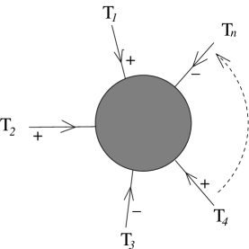
Figure 1: A scattering amplitude of $n$ gluons in Yang-Mills theory. Each gluon comes with the color factor $T_{i},$ spinors $\lambda_{i},\tilde{\lambda}_{i}$ and helicity label $h_{i}=\pm 1.$

2.3 Maximally Helicity Violating Amplitudes

To make the discussion more concrete, we consider tree level scattering of $n$ gluons in Yang-Mills theory. These amplitudes are of phenomenological importance. The multijet production at LHC will be dominated by tree level QCD scattering.

Consider Yang-Mills theory with gauge group $U(N).$ Recall that tree level scattering amplitudes are planar and lead to single trace interactions. In an index loop, the gluons are attached in a definite cyclic order, say $1,2,\dots,n.$ Then the amplitude comes with a group theory factor $\mathop{\rm Tr}\nolimits T_{1}T_{2}\dots T_{n}.$ It is sufficient to give the amplitude with one cyclic order. The full amplitude is obtained from this by summing over the cyclic permutations to achieve Bose symmetry

$$A=g^{n-2}(2\pi)^{4}\delta^{4}\left(\sum_{i}^{n}p_{i}\right){\cal A}(1,2,\dots,n)\mathop{\rm Tr}\nolimits(T_{1}T_{2}\dots T_{n})\,+\,permutations.$$ (30)

Here, $g$ is the coupling constant of the gauge theory. In the rest of the lecture notes, we will always consider gluons in the cyclic order $1,2,\dots,n$ and we will omit the group theory factor and the delta function of momentum conservation in writing the formulas. Hence we will consider the ‘reduced color ordered amplitude’ ${\cal A}(1,2,\dots,n).$

The scattering amplitude with $n$ incoming gluons of the same helicity vanishes. So does the amplitude, for $n\geq 3,$ with $n-1$ incoming gluons of one helicity and one of the opposite helicity. The first nonzero amplitudes, the maximally helicity violating (MHV) amplitudes, have $n-2$ gluons of one helicity and two gluons of the other helicity. Suppose that gluons $r,s$ have negative helicity and the rest of gluons have positive helicity. Then the tree level amplitude, stripped of the momentum delta function and the group theory factor, is

$${\cal A}(r^{-},s^{-})=g^{n-2}\frac{\langle{\lambda_{r},\lambda_{s}}\rangle^{4}}{\prod_{k=1}^{n}\langle{\lambda_{k},\lambda_{k+1}}\rangle}.$$ (31)

The amplitude ${\cal A}(r^{+},s^{+})$ with gluons $r,s$ of positive helicity and the rest of the gluons of negative helicity follows from (31) by exchange $\langle{}\rangle\leftrightarrow[].$ Note, that the amplitude has the correct homogeneity in each variable. It is homogeneous of degree $-2$ in $\lambda_{i}$ for positive helicity gluons; and of degree $-2$ for negative helicity gluons $i=r,s$ as required by the auxiliary condition (28). The amplitude ${\cal A}$ is sometimes called ‘holomorphic’ because it depends on the ‘holomorphic’ spinors $\lambda_{i}$ only.

3 Twistor Space

3.1 Conformal Invariance of Scattering Amplitudes

Before discussing twistor space, let us show the conformal invariance of the MHV tree level amplitude. Firstly, we need to construct representation of the conformal group generators in terms of the spinors $\lambda,\tilde{\lambda}.$ We will consider the conformal generators for a single particle. The generators of the $n$-particle system are given by the sum of the generators over the $n$ particles.

Some of the generators are clear. The Lorentz generators are the first order differential operators

$$J_{ab} = \frac{i}{2}\left(\lambda_{a}\frac{\partial}{\partial\lambda^{b}}+\lambda_{b}\frac{\partial}{\partial\lambda^{a}}\right)$$ (32)

$$\tilde{J}_{\dot{a}\dot{b}} = \frac{i}{2}\left(\tilde{\lambda}_{\dot{a}}\frac{\partial}{\partial\tilde{\lambda}^{\dot{b}}}+\tilde{\lambda}_{\dot{b}}\frac{\partial}{\partial\tilde{\lambda}^{\dot{a}}}\right).$$ (33)

The momentum operator is the multiplication operator

$$P_{a\dot{a}}=\lambda_{a}\tilde{\lambda}_{\dot{a}}.$$ (34)

The remaining generators are the dilatation operator $D$ and the generator of special conformal transformation $K_{a\dot{a}}.$ The commutation relations of the dilatation operator are

$$[D,P]=iP,\qquad[D,K]=-iK,$$ (35)

so $P$ has dimension $+1$ and $K$ has dimension $-1.$ We see from (34) that it is natural to take $\lambda$ and $\tilde{\lambda}$ to have dimension $1/2.$ Hence, a natural guess for the special conformal generator respecting all the symmetries is

$$K_{a\dot{a}}=\frac{\partial^{2}}{\partial\lambda^{a}\partial\tilde{\lambda}^{\dot{a}}}.$$ (36)

We find the dilatation operator $D$ from the closure of the conformal algebra. The commutation relation

$$[K_{a\dot{a}},P^{b\dot{b}}]=-i\left(\delta_{a}{}^{b}\tilde{J}_{\dot{a}}{}^{\dot{b}}+\delta_{\dot{a}}{}^{\dot{b}}J_{a}{}^{b}+\delta_{a}{}^{b}\delta_{\dot{a}}{}^{\dot{b}}D\right)$$ (37)

determines the dilatation operator to be

$$D=\frac{i}{2}\left(\lambda^{a}\frac{\partial}{\partial\lambda^{a}}+\tilde{\lambda}^{\dot{a}}\frac{\partial}{\partial\tilde{\lambda}^{\dot{a}}}+2\right).$$ (38)

We are now ready to verify that the MHV amplitude

$${\cal A}(r^{-},s^{-})=(2\pi)^{4}\delta^{4}\left(\sum_{i}\lambda_{i}^{a}\tilde{\lambda}^{\dot{a}}_{i}\right)\frac{\langle{\lambda_{r},\lambda_{s}}\rangle^{4}}{\prod_{k=1}^{n}\langle{\lambda_{k},\lambda_{k+1}}\rangle},$$ (39)

is invariant under the conformal group. The Lorentz generators are clearly symmetries of the amplitude. The momentum operator annihilates the amplitude thanks to the delta function of momentum conservation.

It remains to verify that the amplitude is annihilated by $D$ and $K.$ For simplicity, we will only consider the dilatation operator $D.$ The numerator contains the delta function of momentum conservation which has dimension $D=-4$ and the factor $\langle{\lambda_{r},\lambda_{s}}\rangle^{4}$ of dimension $4.$ Hence, $D$ commutes with the numerator. So we are left with the denominator

$$\frac{1}{\prod_{k=1}^{n}\langle{\lambda_{k},\lambda_{k+1}}\rangle}.$$ (40)

This is annihilated by $D_{k}$ for each particle $k,$ since the $-2$ coming from the second power of $\lambda_{k}$ in the denominator gets cancelled against the $+2$ from the definition of the dilatation operator (38).

3.2 Transform to Twistor Space

We have demonstrated conformal invariance of the MHV amplitude, however the representation of the conformal group that we have encountered above is quite exotic. The Lorentz generators are first order differential operators, but the momentum is a multiplication operator and the special conformal generator is a second order differential operator.

We can put the action of the conformal group into a more standard form if we make the following transformation

$$\tilde{\lambda}_{\dot{a}} \rightarrow i\frac{\partial}{\partial\mu^{\dot{a}}}$$ (41)

$$\frac{\partial}{\partial\tilde{\lambda}^{\dot{a}}} \rightarrow i\mu_{\dot{a}}.$$ (42)

Making this substitution we have arbitrarily chosen to Fourier transform $\tilde{\lambda}$ rather than $\lambda.$ This choice breaks the symmetry between positive and negative helicities. The amplitude with $n_{1}$ positive helicity and $n_{2}$ negative helicity gluons has different description in twistor space from an amplitude with $n_{2}$ positive helicity gluons and $n_{1}$ negative helicity gluons.

Upon making this substitution, all operators become first order. The Lorentz generators take the form

$$J_{ab} = \frac{i}{2}\left(\lambda_{a}\frac{\partial}{\partial\lambda^{b}}+\lambda_{b}\frac{\partial}{\partial\lambda^{a}}\right)$$ (43)

$$\tilde{J}_{\dot{a}\dot{b}} = \frac{i}{2}\left(\mu_{\dot{a}}\frac{\partial}{\partial\mu^{\dot{b}}}+\mu_{\dot{b}}\frac{\partial}{\partial\mu^{\dot{a}}}\right).$$ (44)

The momentum and special conformal operators become

$$P_{a\dot{a}} = i\lambda_{a}\frac{\partial}{\partial\mu^{\dot{a}}}$$ (45)

$$K_{a\dot{a}} = i\mu_{\dot{a}}\frac{\partial}{\partial\lambda^{a}}.$$ (46)

Finally, the dilatation operator (38) becomes a homogeneous first order operator

$$D=\frac{i}{2}\left(\lambda^{a}{\partial\over\partial\lambda^{a}}-\mu^{\dot{a}}\frac{\partial}{\partial\mu^{\dot{a}}}\right).$$ (47)

This representation of the four dimensional conformal group is easy to explain. The conformal group of Minkowski space is $SO(4,2)$ which is the same as $SU(2,2).$ $SU(2,2),$ or its complexification $Sl(4,{C}),$ has an obvious four-dimensional representation acting on

$$Z^{I}=(\lambda^{a},\mu^{\dot{a}}).$$ (48)

$Z^{I}$ is called a twistor and the space ${C}^{4}$ spanned by $Z^{I}$ is called the twistor space. The action of $Sl(4,{C})$ on the $Z^{I}$ is generated by $15$ traceless matrices $\Lambda^{I}{}_{J},\ I,J=1,\dots,4,$ that correspond to the $15$ first order operators $J_{ab},\tilde{J}_{\dot{a}\dot{b}},D,P_{a\dot{a}},K_{a\dot{a}}.$

If we are in signature $++--,$ the conformal group is $SO(3,3)\cong Sl(4,{R}).$ The twistor space is a copy of ${R}^{4}$ and we can consider $\lambda$ and $\mu$ to be real. In the Euclidean signature $++++$, the conformal group is $SO(5,1)\cong SU^{\ast}(4)$ where $SU^{\ast}(4)$ is the noncompact version of $SU(4),$ so we must think of twistor space as a copy of ${C}^{4}.$

For signature $++--,$ where $\tilde{\lambda}$ is real, the transformation from momentum space scattering amplitudes to twistor space scattering amplitudes is made by a simple Fourier transform that is familiar from quantum mechanics

$$\tilde{\cal A}(\lambda_{i},\mu_{i})=\int\prod_{j=1}^{n}{d^{2}\tilde{\lambda}_{j}\over(2\pi)^{2}}\exp(i[\mu_{j},\tilde{\lambda}_{j}]){\cal A}(\lambda_{i},\tilde{\lambda}_{i}).$$ (49)

The same Fourier transform turns a momentum space wavefunction $\psi(\lambda,\tilde{\lambda})$ to a twistor space wavefunction

$$\tilde{\psi}(\lambda,\mu)=\int{d^{2}\tilde{\lambda}\over(2\pi)^{2}}\exp(i[\mu,\tilde{\lambda}])\psi(\lambda,\tilde{\lambda}).$$ (50)

Recall that the scattering amplitude of massless particles obeys the auxiliary condition

$$\left(\lambda^{a}_{i}\frac{\partial}{\partial\lambda^{a}_{i}}-\tilde{\lambda}_{i}^{\dot{a}}\frac{\partial}{\partial\tilde{\lambda}^{\dot{a}}_{i}}\right){\cal A}(\lambda_{i},\tilde{\lambda}_{i},h_{i})=-2h_{i}{\cal A}(\lambda_{i},\tilde{\lambda}_{i},h_{i})$$ (51)

for each particle $i,$ with helicity $h_{i}.$ In terms of $\lambda_{i}$ and $\mu_{i},$ this becomes

$$\left(\lambda^{a}_{i}\frac{\partial}{\partial\lambda^{a}_{i}}+\mu_{i}^{\dot{a}}\frac{\partial}{\partial\mu^{\dot{a}}_{i}}\right)\tilde{\cal A}(\lambda_{i},\mu_{i},h_{i})=-(2h_{i}+2)\tilde{\cal A}(\lambda_{i},\mu_{i},h_{i}).$$ (52)

There is a similar condition for the twistor wavefunctions of particles. The operator on the left hand side coincides with $Z^{I}{\partial\over\partial Z^{I}}$ that generates the scaling of the twistor coordinates

$$Z^{I}\rightarrow tZ^{I},\qquad t\in{C}^{\ast}.$$ (53)

So the wavefunctions and scattering amplitudes have known behavior under the ${C}^{\ast}$ action $Z^{I}\rightarrow tZ^{I}.$ Hence, we can identify the sets of $Z^{I}$ that differ by the scaling $Z^{I}\rightarrow tZ^{I}$ and throw away the point $Z^{I}=0.$ We get the projective twistor space ${CP}^{3}$ or ${RP}^{3}$ if $Z^{I}$ are complex or real-valued. The $Z^{I}$ are the homogeneous coordinates on the projective twistor space. It follows from (52) that, the scattering amplitudes are homogeneous functions of degree $-2h_{i}-2$ in the twistor coordinates $Z_{i}^{I}$ of each particle particle. In the complex case, this means that scattering amplitudes are sections of the complex line bundle ${\cal O}(-2h_{i}-2)$ over a ${CP}^{3}_{i}$ for each particle. For further details on twistor transform, see any standard textbook on twistor theory, e.g. [52, 4].

3.3 Scattering Amplitudes in Twistor Space

In an $n$ gluon scattering process, after the Fourier transform into twistor space, the external gluons are associated with points $P_{i}$ in the projective twistor space. The scattering amplitudes are functions of the twistors $P_{i},$ that is, they are functions defined on the product of $n$ copies of twistor space, one for each particle.

Let us see what happens to the tree level MHV amplitude with $n-2$ gluons of positive helicity and $2$ gluons of negative helicity, after Fourier transform into twistor space. We work in $++--$ signature, for which the twistor space is a copy of ${RP}^{3}.$ The advantage of $++--$ signature is that the transform to twistor space is an ordinary Fourier transform and the scattering amplitudes are ordinary functions on a product of ${RP}^{3}$’s, one for each particle. With other signatures, the twistor transform involves $\overline{\partial}$-cohomology and other mathematical machinery.

We recall that the MHV amplitude with negative helicity gluons $r,s$ is

$$A(\lambda_{i},\tilde{\lambda}_{i})=(2\pi)^{4}\delta^{4}(\sum_{i}\lambda_{i}\tilde{\lambda}_{i})f(\lambda_{i}),$$ (54)

where

$$f(\lambda_{i})=g^{n-2}{\langle{\lambda_{r},\lambda_{s}}\rangle^{4}\over\prod_{k}\langle{\lambda_{k},\lambda_{k+1}}\rangle}.$$ (55)

The only property of $f(\lambda_{i}),$ that we need is that it is a function of the holomorphic spinors $\lambda_{i}$ only. It does not depend on the anti-holomorphic spinors $\tilde{\lambda}_{i}.$

We express the delta function of momentum conservation as an integral

$$(2\pi)^{4}\delta^{4}(\sum_{i}\lambda_{i}^{a}\tilde{\lambda}_{i}^{\dot{a}})=\int d^{4}x^{a\dot{a}}\exp\left(ix_{b\dot{b}}\sum_{i}\lambda_{i}^{b}\tilde{\lambda}_{i}^{\dot{b}}\right).$$ (56)

Hence, we can rewrite the amplitude as

$$A(\lambda_{i},\tilde{\lambda}_{i})=\int d^{4}x\exp\left(ix_{b\dot{b}}\sum_{i}\lambda_{i}^{b}\tilde{\lambda}_{i}^{\dot{b}}\right)f(\lambda_{i}).$$ (57)

To transform the amplitude into twistor space, we simply carry out a Fourier transform with respect to all $\tilde{\lambda}$’s. Hence, the twistor space amplitude is

$$A(\lambda_{i},\mu_{i})=\int{d^{2}\tilde{\lambda}_{1}\over(2\pi)^{2}}\dots d^{2}\tilde{\lambda}_{n}\over(2\pi)^{2}\exp\left(i\sum_{j=1}^{n}\mu_{j\dot{a}}\tilde{\lambda}_{j}^{\dot{a}}\right)\int d^{4}x\,\exp\left(ix_{b\dot{b}}\sum_{j}\lambda_{j}^{b}\tilde{\lambda}_{j}^{\dot{b}}\right)f(\lambda_{i}).$$ (58)

The only dependece on $\tilde{\lambda}_{i}$ is in the exponential factors. Hence the integrals over $\tilde{\lambda}_{j}$ gives a product of delta functions with the result [63]

$$A(\lambda_{i},\mu_{i})=\int d^{4}x\prod_{j=1}^{n}\delta^{2}(\mu_{j\dot{a}}+x_{a\dot{a}}\lambda^{a}_{j})f(\lambda_{i}).$$ (59)

This equation has a simple geometrical interpretation. Pick some $x^{a\dot{a}}$ and consider the equation

$$\mu_{\dot{a}}+x_{a\dot{a}}\lambda^{a}=0.$$ (60)

The solution set for $x=0$ is a ${RP}^{1}$ or ${CP}^{1}$ depending on whether the variables are real or complex. This is true for any $x$ as the equation lets us solve for $\mu_{\dot{a}}$ in terms of $\lambda^{a}.$ So $(\lambda^{1},\lambda^{2})$ are the homogeneous coordinates on the curve.

In real twistor space, which is appropriate for signature $++--,$ the curve ${RP}^{1}$ can be described more intuitively as a straight line, see fig. 2. Indeed, throwing away the set $Z^{1}=0,$ we can describe the rest of ${RP}^{3}$ as a copy of ${R}^{3}$ with the coordinates $x_{i}=Z_{i}/Z_{1},i=2,3,4.$ The equations (60) determine two planes whose intersection is the straight line in question.

In complex twistor space, the genus zero curve ${CP}^{1}$ is topologically a sphere $S^{2}.$ The ${CP}^{1}$ is an example of a holomorphic curve in ${CP}^{3}.$ The simplest holomorphic curves are defined by vanishing of a pair of homogeneous polynomials in the $Z^{I}$

$$f(Z^{1},\dots,Z^{4}) = 0$$ (61)

$$g(Z^{1},\dots,Z^{4}) = 0.$$ (62)

If $f$ is homogeneous of degree $d_{1}$ and $g$ is homogeneous of degree $d_{2},$ the curve has degree $d_{1}d_{2}.$ The equations

$$\mu_{\dot{b}}+x_{b\dot{b}}\lambda^{b}=0,\quad\dot{b}=1,2$$ (63)

are both linear, $d_{1}=d_{2}=1$. Hence the degree of the ${CP}^{1}$ is $d=d_{1}d_{2}=1.$ Moreover, every degree one genus zero curve in ${CP}^{3}$ is of the form (63) for some $x^{b\dot{b}}.$

The area of a holomorphic curve of degree $d,$ using the natural metric on ${CP}^{3},$ is $2\pi d.$ So the curves we found with $d=1$ have the minimal area among nontrivial holomorphic curves. They are associated with the minimal nonzero Yang-Mills tree amplitudes, the MHV amplitudes.

Going back to the amplitude (59), the $\delta$-functions mean that the amplitude vanishes unless $\mu_{j\dot{a}}+x_{a\dot{a}}\lambda^{a}_{j}=0,j=1,\dots n,$ that is, unless some curve of degree one determined by $x_{a\dot{a}}$ contains all $n$ points $(\lambda_{j},\mu_{j}).$ The result is that the MHV amplitudes are supported on genus zero curves of degree one. This is a consequence of the holomorphy of these amplitudes.

Figure 2: (a) In complex twistor space ${CP}^{3}$, the MHV amplitude localizes to a ${CP}^{1}.$ (b) In the real case, the amplitude is associated to a real line in ${R}^{3}.$

The general conjecture is that an $l$-loop amplitude with $p$ gluons of positive helicity and $q$ gluons of negative helicity is supported on a holomorphic curve in twistor space. The degree of the curve is determined by

$$d=q-1+l.$$ (64)

The genus of the curve is bounded by the number of the loops

$$g\leq l.$$ (65)

The MHV amplitudes are a special case of this for $q=2,l=0.$ Indeed the conjecture in this case gives that MHV amplitudes are supported in twistor space on a genus zero curve of degree one.

The natural interpretation of this is that the curve is the worldsheet of a string. In some way of describing the perturbative gauge theory, the amplitudes arise from coupling of the gluons to a string. In the next two sections we discuss a proposal for such a string theory due to Witten [76] in which the strings in questions are D1-strings. There is an alternative version of twistor string theory due to Berkovits [15, 17], discussed in section 7, in which the curves come from fundamental strings. The Berkovits’s twistor string theory seems to give an equivalent description of the scattering amplitudes. Further proposals [65, 3, 7] have not yet been used for computing scattering amplitudes.

4 Twistor String Theory

In this section, we will describe a string theory that gives a natural framework for understanding the twistor properties of scattering amplitudes discussed in previous section. This is a topological string theory whose target space is a supersymmetric version of the twistor space.

4.1 Brief Review of Topological Strings

Firstly, let us consider an ${\cal N}=2$ topological field theory in $D=2$ [74]. The ${\cal N}=2$ supersymmetry algebra has two supersymmetry generators $Q_{i},i=1,2$ that satisfy the anticommutation relations

$$\{Q_{\alpha i},Q_{\beta j}\}=\delta_{ij}\gamma^{\mu}_{\alpha\beta}P_{\mu}.$$ (66)

In two dimensions, the Lorentz group $SO(1,1)$ is generated by the Lorentz boost $L.$ We diagonalize $L$ by going into the light-cone frame $P_{\pm}=P_{0}\pm P_{1},$

$$[L,P_{\pm}] = \pm P_{\pm}$$ (67)

$$\{L,Q_{\pm}\} = \pm\frac{1}{2}Q_{\pm}.$$ (68)

The commutation relations of the ${\cal N}=2$ supersymmetry algebra become

$$\{Q_{+i},Q_{+j}\} = \delta_{ij}P_{+}$$ (69)

$$\{Q_{-i},Q_{-j}\} = \delta_{ij}P_{-}$$ (70)

$$\{Q_{+i},Q_{-j}\} = 0.$$ (71)

We let

$$Q=Q_{+1}+iQ_{+2}+Q_{-1}\pm iQ_{-2}$$ (72)

with either choice of sign. It follows from (69) that $Q$ is nilpotent

$$Q^{2}=0,$$ (73)

so we would like to consider $Q$ as a BRST operator.

However $Q$ (72) is not a scalar so this construction would violate Lorentz invariance. There is a way out if the theory has left and right R-symmetries $R_{+}$ and $R_{-}.$ Under $R_{+},$ the combination of supercharges $Q_{+1}\pm iQ_{+2}$ has charge $\pm 1/2$ and $Q_{-1}\pm iQ_{-2}$ is neutral. For $R_{-},$ the same is true with ‘left’ and ‘right’ interchanged.

Hence, we can make $Q$ scalar if we modify the Lorentz generator $L$ to be

$$L^{\prime}=L-\frac{1}{2}R_{+}\mp\frac{1}{2}R_{-}.$$ (74)

At a more fundamental level, this change in the Lorentz generator arises if we replace the stress tensor $T_{\mu\nu}$ with

$$\tilde{T}_{\mu\nu}=T_{\mu\nu}-\frac{1}{2}(\partial_{\mu}J^{+}_{\nu}+\partial_{\nu}J^{+}_{\mu})\mp\frac{1}{2}(\partial_{\mu}J^{-}_{\nu}+\partial_{\nu}J^{-}_{\mu}),$$ (75)

where $J^{+}_{\nu}$ and $J^{-}_{\mu}$ are the left and right R-symmetry currents. The substitution (75) is usually referred to as ‘twisting’ the stress tensor.

We give a new interpretation to the theory by taking $Q$ to be a BRST operator. A state $\Psi$ is considered to be physical if it is annihilated by $Q$

$$Q\Psi=0.$$ (76)

Two states $\Psi$ and $\Psi^{\prime}$ are equivalent if

$$\Psi-\Psi^{\prime}=Q\Phi,$$ (77)

for some $\Phi.$ Similarly, we take the physical operators to commute with the BRST charge

$$[Q,{\cal O}]=0.$$ (78)

Two operators are equivalent if they differ by an anticommutator of $Q,$

$${\cal O}^{\prime}\sim{\cal O}+\{Q,{\cal V}\},$$ (79)

for some operator ${\cal V}.$

The theory with the stress tensor $\tilde{T}_{\mu\nu}$ and BRST operator $Q$ is called a topological field theory. The basis for the name is that one can use the supersymmetry algebra to show that the twisted stress tensor is BRST trivial

$$\tilde{T}_{\mu\nu}=\{Q,\Lambda_{\mu\nu}\}.$$ (80)

It follows that in some sense the worldsheet metric is irrelevant. The correlation function

$$\langle{{\cal O}_{1}(x_{1}){\cal O}_{2}(x_{2})\dots\cal O_{n}(x_{n})}\rangle_{\Sigma}$$ (81)

of physical operators ${\cal O}_{i}$ obeying $[Q,{\cal O}_{i}]=0$ on a fixed Riemann surface $\Sigma$ is independent of metric on $\Sigma.$ Indeed, varying the metric $g_{\mu\nu}\rightarrow g_{\mu\nu}+\delta g_{\mu\nu},$ the correlation function stays the same up to BRST trivial terms

$$\langle{{\cal O}_{1}(x_{1})\dots\cal O_{n}(x_{n})\int_{\Sigma}\delta(\sqrt{g}g^{\mu\nu})\tilde{T}_{\mu\nu}}\rangle=\langle{{\cal O}_{1}(x_{1})\dots\cal O_{n}(x_{n})\int_{\Sigma}\delta(\sqrt{g}g^{\mu\nu})\{Q,\Lambda_{\mu\nu}\}}\rangle=0.$$ (82)

More importantly for us, we can also construct a topological string theory in which one obtains the correlation functions by integrating (81) over the moduli of the Riemann surface $\Sigma$ using $\Lambda_{\mu\nu}$ where the antighost $b_{\mu\nu}$ usually appears in the definition of the string measure.

For an ${\cal N}=2$ supersymmetric field theory in two dimensions with anomaly-free left and right R-symmetries we get two topological string theories, depending on the choice of sign in (72). We would like to consider the case that the ${\cal N}=2$ model is a sigma model with a target space being a complex manifold $X.$ In this case, the two R-symmetries exist classically, so classically we can construct the two topological string theories, called the A-model and the B-model. Quantum mechanically, however, there is an anomaly, and the B-model only exists if $X$ is a Calabi-Yau manifold.

4.2 Open String B-model on a Super-Twistor Space

To define open strings in the B-model, one needs BRST invariant boundary conditions. The simplest such conditions are Neumann boundary conditions [75]. Putting in $N$ space filling D5-branes gives $Gl(n,{C})$ (whose compact real form is $U(N)$) gauge symmetry. The zero modes of the D5-D5 strings give a $(0,1)$ form gauge field $A=A_{\overline{i}}dz^{\overline{i}}$ in the target space. The BRST operator acts as the $\overline{\partial}$ operator and the string $\ast$ product is just the wedge product. Hence, $A$ is subject to the gauge invariance

$$\delta A=Q\epsilon=\overline{\partial}\epsilon+[A,\epsilon],$$ (83)

and the string field theory action reduces to the action of the holomorphic Chern-Simons theory [75]

$$S={1\over 2}\int\Omega\wedge\mathop{\rm Tr}\nolimits\left(A\wedge\overline{\partial}A+{2\over 3}A\wedge A\wedge A\right),$$ (84)

where $\Omega$ is the Calabi-Yau volume form.

We would like to consider the open string B-model with target space ${CP}^{3},$ but we cannot, since ${CP}^{3}$ is not a Calabi-Yau manifold and the B-model is well defined only on a Calabi-Yau manifold. On a non-Calabi-Yau manifold, the R-symmetry that we used to twist the stress tensor is anomalous. A way out is to introduce spacetime supersymmetry. Instead of ${CP}^{3},$ which has homogeneous coordinates $Z^{I},I=1,\dots,4$ we consider a supermanifold ${CP}^{3|N}$ with bosonic and fermionic coordinates

$$Z^{I},\quad\psi^{A}\qquad I=1,\dots,4,\quad A=1,\dots,N,$$ (85)

with identification of two sets of coordinates that differ by a scaling

$$(Z^{I},\psi^{A})\cong(tZ^{I},t\psi^{A})\qquad t\in{C}^{\ast}.$$ (86)

The ${CP}^{3|N}$ is a Calabi-Yau supermanifold if and only if the number of fermionic dimensions is $N=4.$ To see this, we construct the holomorphic measure on ${CP}^{3|4}.$ We start with the $(4|N)$ form on ${C}^{4|N}$

$$\Omega_{0}=dZ^{1}\dots dZ^{4}d\psi^{1}\dots d\psi^{N}$$ (87)

and study its behavior under the rescaling symmetry (86). For this, recall that $d\psi$ scales oppositely to $\psi$

$$(dZ^{I},d\psi^{A})\rightarrow(tdZ^{I},t^{-1}d\psi^{A}).$$ (88)

It follows, that $\Omega_{0}$ is ${C}^{\ast}$ invariant if and only if $N=4.$ In this case we can divide by the $C^{\ast}$ action and get a Calabi-Yau measure on ${CP}^{3|4}$

$$\Omega={1\over 4!}\epsilon_{IJKL}Z^{I}dZ^{J}dZ^{K}dZ^{L}{1\over 4!}\epsilon_{ABCD}\psi^{A}\psi^{B}\psi^{C}\psi^{D}.$$ (89)

The twistor space ${CP}^{3}$ has a natural $Sl(4,{C})$ group action that acts as $Z^{A}\rightarrow\Lambda^{A}{}_{B}Z^{B}$ on the homogeneous coordinates of ${CP}^{3}$. The real form $SU(2,2)$ of $Sl(4,{C})$ is the conformal group of Minkowski space. Similarly, the super-twistor space ${CP}^{3|N}$ has a natural $Sl(4|N,{C})$ symmetry. The real form $SU(2,2|N)$ of this is the superconformal symmetry group with $N$ supersymmetries.

For $N=4$, the superconformal group $SU(2,2|4)$ is the symmetry group of ${\cal N}=4$ super-Yang-Mills theory. In a sense, this is the simplest non-abelian gauge theory in four dimensions. The ${\cal N}=4$ superconformal symmetry uniquely determines the states and interactions of the gauge theory. In particular, the beta function of ${\cal N}=4$ gauge theory vanishes.

Now we know a new reason for ${\cal N}=4$ to be special. The topological B-model on ${CP}^{3|N}$ exists if and only if ${\cal N}=4.$ The B-model on ${CP}^{3|4}$ has a $SU(2,2|4)$ symmetry coming from the geometric transformations of the twistor space. This is related via the twistor transform to the ${\cal N}=4$ superconformal symmetry.

In the topological B-model with space-filling branes on ${CP}^{3|4}$, the basic field is the holomorphic gauge field ${\cal A}={\cal A}_{\overline{I}}dZ^{\overline{I}}$,

$${\cal A}(Z,\overline{Z},\psi)=A(Z,\overline{Z})+\psi^{A}\xi_{A}(Z,\overline{Z})+{1\over 2!}\psi^{A}\psi^{B}\psi_{AB}(Z,\overline{Z})+\dots+{1\over 4!}\epsilon_{ABCD}\psi^{A}\psi^{B}\psi^{C}\psi^{D}G(Z,\overline{Z}).$$ (90)

The action is the same as (84), except that the gauge field ${\cal A}$ now depends on $\psi$

$$S=\frac{1}{2}\int\Omega\wedge\mathop{\rm Tr}\nolimits\left({\cal A}\overline{\partial}{\cal A}+{2\over 3}{\cal A}\wedge{\cal A}\wedge{\cal A}\right),$$ (91)

and the holomorphic three form is (89). The classical equations of motions obtained from (91) are

$$\overline{\partial}{\cal A}+{\cal A}\wedge{\cal A}=0.$$ (92)

Linearizing the equations of motions around the trivial solutions ${\cal A}=0,$ they tell us that

$$\overline{\partial}\Phi=0,$$ (93)

where $\Phi$ is any of the components of ${\cal A}.$ The gauge invariance reduces to $\delta\Phi=\overline{\partial}\alpha.$ Hence for each component $\Phi,$ the field $\Phi$ defines an element of a cohomology group.

This action has the amazing property that its spectrum is the same as that of ${\cal N}=4$ super Yang-Mills theory in Minkowski space. To see this, we need to use that the elements of $(0,1)$ cohomology groups of degree $2h-2$ are related by twistor transform to helicity $h$ free fields on Minkowski space.

To figure out the degrees of various components ${\cal A}$, notice that the action must be invariant under the ${C}^{*}$ action $Z^{I}\rightarrow tZ^{I}.$ Since the holomorphic measure is also invariant under the scaling, the only way that the action (91) is invariant is that the superfield ${\cal A}$ is also invariant, in other words, ${\cal A}$ is of degree zero

$${\cal A}\in H^{0,1}({CP}^{3|4},{\cal O}(0)).$$ (94)

Looking back at the expansion (90) of the superfield, we identify the components, via the twistor correspondence, with fields in Minkowski space of definite helicity. $A$ is is of degree zero, just like the superfield ${\cal A}.$ Hence, it is related by twistor transform to a field of helicity $+1.$ The field $G$ has degree $-4$ to off-set the degree $4$ coming the four $\psi$, so it corresponds to a field of helicity $-1.$ Continuing in this fashion, we obtain the complete spectrum of ${\cal N}=4$ supersymmetric Yang-Mills theory. The twistor fields $A,\xi_{A},\phi_{AB},\xi_{ABC},G$ describe, via twistor transform, particles of helicities $1,+\frac{1}{2},0,-\frac{1}{2},-1$ respectively.

The fields also have the correct representations under the $SU(4)$ R-symmetry group. This symmetry is realized in twistor space by the natural geometric action on the fermionic coordinates $\psi^{A}\rightarrow\Lambda^{A}{}_{B}\psi^{B}.$ Hence, $\psi^{A}$ transforms in the $\bf 4$ of the $SU(4)_{R}.$ The holomorphic gauge superfield ${\cal A}(Z,\psi)$ is invariant under the R-symmetry, hence the representations of the components of ${\cal A}$ must be conjugate to the representations of the $\psi$ factors that they multiply in (90). Hence, $A,\xi_{A},\phi_{AB},\xi_{ABC}$ and $G$ transform in the $\bf 1,\overline{4},6,4,1$ representation of $SU(4)_{R}$ respectively

4.3 D-Instantons

The action (91) also describes some of the interactions of ${\cal N}=4$ super Yang-Mills, but not all. It cannot describe the full interactions, because an extra $U(1)$ R-symmetry gets in the way. The fermionic coordinates $\psi^{A},A=1,\dots,4$ have an extra $U(1)_{R}$ besides the $SU(4)_{R}$ considered above. Indeed, the full R-symmetry group in twistor space is

$$U(4)_{R}=SU(4)_{R}\times U(1)_{R},$$ (95)

where we take the extra $U(1)_{R}$, which we call $S,$ to rotate the fermions by a common phase

$$S:\ Z^{I}\rightarrow Z^{I},\quad\psi^{A}\rightarrow e^{i\theta}\psi^{A}.$$ (96)

In the B-model, the extra $U(1)_{R}$ is anomalous, since it does not leave fixed the holomorphic measure $\Omega\sim d^{3}Zd\psi^{1}\dots d\psi^{4}.$ Under the $S$ transformation, the holomorphic measure transforms as $\Omega\rightarrow e^{-4i\theta}\Omega$, so it has charge $S=-4$, hence the $B$-model action has $S=-4.$

However, as we have set things up so far, the anomaly of the B-model is too trivial to agree with the anomaly of ${\cal N}=4$ Yang-Mills theory. With the normalization (96), the $S$ charges of fields are given by their degrees. The ${\cal N}=4$ Yang-Mills action is a sum of terms with $S=-4$ and $S=-8.$ For illustration, consider the positive and negative helicity gluons that have $S$-charge $0$ and $-4$ respectively. The kinetic term and the $++-$ three-gluon vertex contribute to the $S=-4$ part of the Yang-Mills action. The $--+$ and the $--++$ vertices contribute to the $S=-8$ part.

The action of the open string B-model (91) has $S=-4$ coming from the anomaly of $S$ of the holomorphic measure $\Omega$. To get the $S=-8$ piece of the Yang-Mills action, we need to enrich the B-model with nonperturbative instanton contributions.

The instantons in question are Euclidean D1-branes wrapped on holomorphic curves in ${CP}^{3|4}$ on which open string can end. The gauge theory amplitudes come from coupling of the open strings to the D1-branes. The massless modes on the worldvolume of a D-instanton are a $U(1)$ gauge field and the modes that describe the motion of the instanton. In the following, we will study mostly tree level amplitudes. These get contributions from genus zero instantons on which the $U(1)$ line bundles have a fixed degree $d=-1$. Hence the bundles do not have any discrete or continuous moduli, so we will ignore the $U(1)$ gauge field from now on. The modes describing the motion of the D-instanton make up the moduli space ${\cal M}$ of holomorphic curves $C$ in the twistor space. To construct scattering amplitudes we need to integrate over ${\cal M}.$

5 Tree Level Amplitudes from Twistor String Theory

5.1 Basic Setup

Recall that the interactions of the full gauge theory come from Euclidean D1-brane instantons on which the open strings can end. The open strings are described by the holomorphic gauge field ${\cal A}.$ To find the coupling of the open strings to the D-instantons, let us consider the effective action of the D1-D5 and D5-D1 strings. Quantizing the zero modes of the D1-D5 strings leads to a fermionic zero form field $\alpha^{i}$ living on the worldvolume of the D-instanton. $\alpha^{i}$ transforms in the fundamental representation of the $Gl(n,{C})$ gauge group coming from the Chan-Paton factors. The D5-D1 strings are described by a fermion $\beta_{i}$ transforming in the antifundamental representation. The kinetic operator for the topological strings is the BRST operator $Q,$ which acts as $\overline{\partial}$ on the low energy modes. So the effective action of the D1-D5 strings is

$$S=\int_{C}\beta(\overline{\partial}+{\cal A})\alpha,$$ (97)

where $C$ is the holomorphic curve wrapped by the D-instanton. From this we read off the vertex operator for an open string with wavefunction $\phi={\cal A}_{\overline{I}}dZ^{\overline{I}}$

$$V_{\phi}=\int_{C}J\wedge\phi,$$ (98)

where $J_{i}{}^{j}=\beta_{i}\alpha^{j}dz$ is a holomorphic current made from the free fermions $\alpha^{j},\beta_{i}$. These currents generate a current algebra on the worldvolume of the D-instanton.

To compute a scattering amplitude, we evaluate the correlation function

$${\cal A}=\int d{\cal M}\langle{V_{\phi_{1}}V_{\phi_{2}}\dots V_{\phi_{n}}}\rangle=\int d{\cal M}\left\langle\int_{C}J_{1}\phi_{1}\dots\int_{C}J_{n}\phi_{n}\right\rangle.$$ (99)

We can think of this as integrating out the fermions $\alpha,\beta$ living on the D-instanton. Hence, the generating function for scattering amplitudes is simply the integral of Dirac operator over moduli space of D-instantons

$$\int d{\cal M}\det(\overline{\partial}+A).$$ (100)

Here, $d{\cal M}$ is the holomorphic measure on the moduli space of holomorphic curves of genus zero and degree $d.$ In topological B-model, the action is holomorphic function of the fields and all path integrals are contour integral. Hence, the integral is actually over a middle-dimensional Lagrangian cycle in the moduli space. This integral is a higher dimensional generalization of the familiar contour integral from complex analysis.

The correlator of the currents on D1-instanton

$$\langle J_{1}(z_{1})J_{2}(z_{2})\dots J_{n}(z_{n})\rangle={\mathop{\rm Tr}\nolimits(T_{1}T_{2}\dots T_{n})dz_{1}dz_{2}\dots dz_{n}\over(z_{1}-z_{2})(z_{2}-z_{3})\dots(z_{n}-z_{1})}+\,permutations$$ (101)

follows from the free fermion correlator on a sphere

$$\alpha^{i}(z)\beta_{j}(z^{\prime})\sim{\delta^{i}{}_{j}\over z-z^{\prime}}.$$ (102)

Scattering Wavefunctions

We would like to compute the scattering amplitudes of plane waves $\phi(x)=\exp\,(i\,p\cdot x)=\exp\,(i\,\pi^{a}\tilde{\pi}^{\dot{a}}x_{a\dot{a}}).$ These are wavefunctions of external particles with definite momentum ${p^{a\dot{a}}=\pi^{a}\tilde{\pi}^{\dot{a}}}.$ The twistor wavefunctions corresponding to plane waves are

$$\phi(\lambda,\mu,\psi)=\overline{\delta}(\langle{\lambda,\pi}\rangle)\exp(i[{\tilde{\pi}},\mu])g(\psi),$$ (103)

where $g(\psi)$ encodes the dependence on fermionic coordinates. For a positive helicity gluon $g(\psi)=1$ and for a negative helicity gluon $g(\psi)=\psi^{1}\psi^{2}\psi^{3}\psi^{4}.$ Here, we have introduced the holomorphic delta function

$$\overline{\delta}(f)=\overline{\partial}\overline{f}\delta^{2}(f),$$ (104)

which is a closed $(0,1)$ form. We normalize it so that for any function $f(z)$, we have

$$\int dz\,\overline{\delta}(z-a)f(z)=f(a).$$ (105)

The idea of (103) is that the delta function $\delta(\langle{\lambda,\pi}\rangle)$ sets $\lambda^{a}$ equal to $\pi^{a}.$ The Fourier transform of the exponential $\exp(i[{\tilde{\pi}},\mu])$ back into Minkowski space gives another delta function that sets $\tilde{\lambda}^{\dot{a}}$ equal to $\tilde{\pi}^{\dot{a}}.$ The twistor string computation with these wavefunctions gives directly momentum space scattering amplitudes.

Actually, the wavefunctions should be modified slightly so that they are invariant under the scaling of the homogeneous coordinates of ${CP}^{3|4}.$ From the basic properties of delta functions, it follows that $\overline{\delta}(\langle{\lambda,\pi}\rangle)$ is homogeneous of degree $-1$ in both $\lambda$ and $\pi.$ Hence, for positive helicity gluons, the wavefunction is actually

$$\phi^{+}(\lambda,\mu)=\overline{\delta}(\langle{\lambda,\pi}\rangle)(\lambda/\pi)\exp\big{(}i[{\tilde{\pi}},\mu](\pi/\lambda)\big{)}.$$ (106)

Here, $\lambda/\pi$ is a well defined holomorphic function, since $\lambda$ is a multiple of $\pi$ on the support of the delta function. The power of $(\lambda/\pi)$ was chosen, so that the wavefunction is homogeneous of degree zero in overall scaling of $\lambda,\mu,\psi.$ Under the scaling

$$(\pi,\tilde{\pi})\rightarrow(t\pi,t^{-1}\tilde{\pi}),$$ (107)

the wavefunction is homogeneous of degree $-2$ as expected for a positive helicity gluon (28). For negative helicity gluon, the wavefunction is

$$\phi^{-}(\lambda,\mu)=\overline{\delta}(\langle{\lambda,\pi}\rangle)(\pi/\lambda)^{3}\exp\big{(}i[\tilde{\pi},\mu](\pi/\lambda)\big{)}\psi^{1}\psi^{2}\psi^{3}\psi^{4}.$$ (108)

Under the scaling (107), the wavefunction is homogeneous of degree $+2$ as expected. For wavefunctions of particles with helicity $h,$ there are similar formulas with $2-2h$ factors of $\psi.$

MHV Amplitudes

We saw in section 3.3 that MHV amplitudes, after Fourier transform into twistor space, localize on genus zero degree one curve $C$, that is, a linearly embedded copy of ${CP}^{1}.$ Here we will evaluate the degree one instanton contribution and confirm that it gives the MHV amplitude.

Consider the moduli space of such curves. Each curve $C$ can be described by the equations

$$\mu^{\dot{a}}=x^{a{\dot{a}}}\lambda_{a}\qquad\psi^{A}=\theta^{Aa}\lambda_{a},$$ (109)

where $\lambda^{a}$ are the homogeneous coordinates and $x^{a\dot{a}}$ and $\theta^{Aa}$ are the moduli of $C$. The holomorphic measure on the moduli space is

$$d{\cal M}=d^{4}xd^{8}\theta.$$ (110)

Hence, the moduli space has $4$ bosonic and $8$ fermionic dimensions.

In terms of the homogeneous coordinate $\lambda^{a}$ the current correlator (101) becomes

$$\langle{J_{1}(\pi_{1})J_{2}(\pi_{2})\dots J_{n}(\pi_{n})}\rangle={\prod_{i}\langle{\lambda_{i},d\lambda_{i}}\rangle\over\langle{\lambda_{1},\lambda_{2}}\rangle\langle{\lambda_{2},\lambda_{3}}\rangle\dots\langle{\lambda_{n},\lambda_{1}}\rangle},$$ (111)

which we found by setting $z_{i}=\lambda^{2}_{i}/\lambda^{1}_{i}$. We stripped away the color factors and kept only the contribution of the term with $1,2,\dots,n$ cyclic order. We multiply this with the wavefunctions $\psi_{i}(\lambda,\mu,\psi)=\overline{\delta}(\langle{\lambda,\pi_{i}}\rangle)\exp\left(i[\mu,\tilde{\pi}_{i}]\right)g_{i}(\psi)$ and integrate over the positions $\lambda_{i},\tilde{\lambda}_{i}$ of the vertex operators. We perform the integral over the positions of the vertex operators using the formula

$$\int_{{CP}^{1}}\langle{\lambda,d\lambda}\rangle\ \overline{\delta}(\langle{\lambda,\pi}\rangle)f(\lambda)=f(\pi),$$ (112)

where $f(\lambda)$ is a homogeneous function of $\lambda^{a}$ of degree $-1.$ This is the homogeneous version of definition of holomorphic delta function

$$\int_{{C}}dz\ \overline{\delta}(z-b)f(z)=f(b).$$ (113)

Hence, each wavefunction contributes a factor of

$$\int_{C}\langle{\lambda,d\lambda}\rangle\phi_{i}=\exp\left(i[\tilde{\pi}_{i},\mu_{i}]\right)g_{i}(\psi_{i}),$$ (114)

where $\mu_{i}^{\dot{a}}=x^{a\dot{a}}\lambda_{ia},\psi^{A}_{i}=\theta^{aA}\lambda_{ia}$ and the delta function sets $\lambda^{a}_{i}=\pi^{a}_{i}$ in the correlation function. So the amplitude becomes

$${\cal A}={1\over\prod_{k}\langle{\pi_{k},\pi_{k+1}}\rangle}\int d^{4}xd^{8}\theta\ \exp\Big{(}i\sum_{k}[\tilde{\pi}_{k},\mu_{k}]\Big{)}\prod_{k}g_{k}(\psi_{k}).$$ (115)

The fermionic part of the wavefunctions is $g_{i}=1$ for the positive helicity gluons and $g_{i}=\psi^{1}_{i}\psi^{2}_{i}\psi^{3}_{i}\psi^{4}_{i}$ for the negative helicity gluons. Since we are integrating over eight fermionic moduli $d^{8}\theta,$ we get nonzero contribution to amplitudes with exactly two negative helicities $r^{-},s^{-}.$ Setting $\psi^{A}=\theta^{Aa}\pi_{a},$ the integral over fermionic dimensions of the moduli space gives the numerator of the MHV amplitude

$$\int d^{8}\theta\prod_{A=1}^{4}\psi_{r}^{A}\prod_{B=1}^{4}\psi_{s}^{B}=\langle{r,s}\rangle^{4}.$$ (116)

Setting $\mu^{\dot{a}}_{i}=x^{a\dot{a}}\pi_{ia},\ i=1,\dots,n,$ the integral over bosonic moduli gives the delta function of momentum conservation

$$\int d^{4}x\exp\left(ix_{a\dot{a}}\sum_{i}\pi_{i}^{a}\tilde{\pi}^{\dot{a}}_{i}\right)=\delta^{4}(\sum_{i=1}^{n}\pi_{i}^{a}\tilde{\pi}_{i}^{\dot{a}}).$$ (117)

Collecting the various pieces, we get the familiar MHV amplitude

$${\cal A}(r^{-},s^{-})={\langle{r,s}\rangle^{4}\over\prod_{i=1}^{n}\langle{i,i+1}\rangle}\delta^{4}(\sum_{i=1}^{n}\pi_{i}\tilde{\pi}_{i}).$$ (118)

5.2 Higher Degree Instantons

Instanton Measure

Here we will construct the measure on the moduli space of genus zero degree $d$ curves. Such curves can be described as degree $d$ maps from an abstract ${CP}^{1}$ with homogeneous coordinates $(u,v)$

$$Z^{I} = P^{I}(u,v)$$ (119)

$$\psi^{A} = \chi^{A}(u,v).$$ (120)

Here $P^{I},\chi^{A}$ are homogeneous polynomials of degree $d$ in $u,v.$ The space of homogeneous polynomials of degree $d$ is a linear space of dimension $d+1,$ spanned by $u^{d},u^{d-1}v,\dots,v^{d}.$ Picking a basis $b^{\alpha}(u,v),\alpha=1,\dots,d+1$, we write

$$P^{I} = \sum_{\alpha}P_{\alpha}^{I}\ b^{\alpha}$$ (121)

$$\psi^{A} = \sum_{\alpha}\chi^{A}_{\alpha}\ b^{\alpha}.$$ (122)

A natural measure is

$$d{\cal M}_{0}=\prod_{\alpha=1}^{d+1}\prod_{A,I=1}^{4}dP^{I}_{\alpha}\ d\chi^{A}_{\alpha}.$$ (123)

This measure is invariant under a general $Gl(d+1,{C})$ transformation of the basis $b_{\alpha}.$ Since the number of bosonic and fermionic coordinates is the same, the Jacobians cancel between fermionic and bosonic parts of the measure. The description (119) is redundant, we need to divide by the ${C}^{\ast}$ action that rescales $P^{I}$ and $\chi^{A}$ by a common factor. This reduces the space of curves from ${C}^{4d+4|4d+4}$ to ${CP}^{4d+3|4d+4}.$ The curve $C$ also stays invariant under an $Sl(2,{C})$ transformation on $(u,v)$ so the actual moduli space of genus zero degree $d$ curves is

$${\cal M}={CP}^{4d+3|4d+4}/Sl(2,{C}).$$ (124)

As $d{\cal M}_{0}$ is $Gl(2,{C})$ invariant, it descends to a holomorphic measure

$$d{\cal M}={d{\cal M}_{0}\over Gl(2,{C})}.$$ (125)

on ${\cal M}.$ Hence, ${\cal M}$ is a Calabi-Yau supermanifold of dimension $(4d|4d+4).$

We can now understand why amplitudes with different helicities come from holomorphic curves of different degrees. Integrating over the moduli space, the measure absorbs $4d+4$ fermion zero modes. These come from the fermionic factors $g(\psi)$ in the wavefunctions of the gluons (103). A positive helicity gluon does not contribute any zero modes while a negative helicity gluon $g^{-}(\psi)=\psi^{1}\psi^{2}\psi^{3}\psi^{4}$ gives $4$ zero modes. Hence, instantons of degree $d$ contribute to amplitudes with $d+1$ negative helicity gluons.

Alternatively, we can get this from counting the $S$ charge anomaly. Wavefunctions of particles with different helicities violate $S$ by different amount. The positive helicity gluons do not violate $S$ while the negative helicity gluons violate $S$ by $-4$ units. So, the amplitudes with $p$ positive helicity gluons and $q$ negative helicity gluons violates the $S$ charge by $-4q$ units.

In the twistor string, there is a source of violation of $S$ from the instanton measure. Since the $S$ charge of $Z$ and $\psi$ is $0$ and $1$ respectively, the charges of the coefficients $P^{I}_{\alpha},\chi^{A}_{\alpha}$ are $0,1.$ Hence, the differentials $dP^{I}_{\alpha},d\chi^{A}_{\alpha}$ have charges $0,-1$ and the $S$ charge of the $(4d|4d+4)$ dimensional measure $d{\cal M}$ is $-4d-4.$

So an instanton can contribute to an amplitude with $q$ negative helicity gluons if and only if

$$d=q-1.$$ (126)

This is the familiar formula discussed at in subsection 3.3. For $l$ loop amplitudes, this relation generalizes to $d=q-1+l.$

Evaluating the Instanton Contribution

Here we consider the connected instanton contribution along the lines of the calculation of the MHV amplitude. The amplitude is [71, 70, 77]

$${\cal A} = \int d{\cal M}_{d}\prod_{i}\int_{C}{\langle{u_{i},du_{i}}\rangle\over\prod_{k}\langle{u_{k},u_{k+1}}\rangle}\overline{\delta}(\langle{\lambda(u_{i}),\pi_{i}}\rangle)\exp\left(i[\mu(u_{i}),\tilde{\pi}_{i}]\right)g_{i}(\psi_{i}).$$ (127)

Here $d{\cal M}_{d}$ is the measure on the moduli space of genus zero degree $d$ curves. Next comes the correlator of currents on the worldvolume of the D1-instanton and the wavefunctions in which we use the parameterization $\lambda^{a}_{i}(u_{i})=P^{a}(u_{i}),\mu^{\dot{a}}(u_{i})=P^{\dot{a}}(u_{i}).$

This is not really an integral. The integral over the $2d+2$ parameters $P^{\dot{a}}_{\alpha}$ gives $2d+2$ delta functions because $P^{\dot{a}}$ appear only in the exponential $\exp\left(\sum_{i}P(u_{i})_{\dot{a}}\tilde{\pi}_{i}^{\dot{a}}\right)$. Hence, we are left with an integral over $4d-(2d+2)+2n=2d+2n-2$ bosonic variables. Here the $2n$ integrals come from the integration over the positions of the vertex operators. Now there are $2n$ delta functions from the wavefunctions since each holomorphic delta function is really a product of two real delta functions $\overline{\delta}(z)=d\overline{z}\ \delta^{2}(z)$, and $2d+2$ delta functions from the integral over the exponentials, which gives a total of $2d+2n+2$. There are four more delta functions than integration variables. The four extra delta functions impose momentum conservation. Hence, the delta functions localize the integral to a sum of contributions from a finite number of points on the moduli space.

Parity Invariance

In the helicity formalism, the parity symmetry of Yang-Mills scattering amplitudes is apparent. The parity changes the signs of the helicities of the gluons. The parity conjugate amplitude can be obtained by simply exchanging $\lambda_{i}$’s with $\tilde{\lambda}_{i}$’s.

To go to twistor space, one Fourier transforms with respect to $\tilde{\lambda}_{i}$, which breaks the symmetry between $\lambda$ and $\tilde{\lambda}.$ Indeed, the result (127) for the scattering amplitude treats $\lambda$ and $\tilde{\lambda}$ asymmetrically. An amplitude with $p$ positive helicities and $q$ negative helicities has contribution from instantons of degree $q-1$, while the parity conjugate amplitude with $q$ gluons of positive helicity and $p$ gluons of negative helicity has contribution from instantons of degree $p-1.$ To show that these two are related by an exchange of $\lambda_{i}$ and $\tilde{\lambda}_{i}$ requires some amount of work. We refer the interested reader to the original literature [71, 70, 77, 17].

Localization on the Moduli Space

Recall that a tree level amplitude with $q$ negative helicity gluons and arbitrary number of positive helicity gluons receives contribution from instantons wrapping holomorphic curves of degree $d=q-1.$ The degree $d$ instanton can consist of several disjoint lower degree instantons whose degrees add up to $d.$ For disconnected scattering amplitudes the instantons are connected by open strings.

Figure 3: An amplitude with tree negative helicity gluons has contribution from two configurations: (a) Connected $d=2$ instanton. (b) Two disjoint $d=1$ instantons. The dashed line represents an open string connecting the instantons.

A priory, one expects that the amplitude receives contributions from all possible instanton configurations with total degree $q-1.$ So for example an amplitude with three negative helicity gluons has contribution from a connected $d=2$ instanton and a contribution from two disjoint $d=1$ instantons, fig. 3.

What one actually finds is that the connected and disconnected instanton contributions reproduce the whole amplitude separately. For example, in the case of amplitude with three negative helicity gluons, it seems that there are two different ways to compute the same amplitude. One can either evaluate it from the connected $d=2$ instantons [71, 70], see fig. 3(a). Alternatively, the amplitude comes from evaluating the contribution of the two disjoint $d=1$ instantons [35], fig. 3(b).

We can explain the equality of various instanton contributions roughly as follows [43]. Consider the connected contribution. The amplitude is expressed as a ‘contour’ integral over a middle-dimensional Lagrangian cycle in the moduli space of degree two curves . The integrand comes from the correlation function on the worldvolume of the D-instanton and from the measure on the moduli space. It has poles in the region of the moduli space, where the instanton degenerates to two intersecting instantons of lower degrees $d_{1}+d_{2}=d$ , fig. 4. Picking a contour that encircles the pole, the integral localizes to an integral over the moduli space ${\cal M}^{\prime}$ of the intersecting lower degree curves.

Similarly, the disconnected contribution has a pole when the two ends of the propagator coincide. This comes from the pole of the open string propagator

$$\overline{\partial}G={\overline{\delta}}^{3}(Z^{\prime}{}^{I}-Z^{I})\delta^{4}(\psi^{\prime}{}^{A}-\psi^{A}).$$ (128)

Hence, the integral over disjoint instantons also localizes on the moduli space of intersecting instantons. It can be shown that the localized integrals coming from either connected or disconnected instanton configurations agree [43] which explains why the connected and disconnected instanton calculations give the entire scattering amplitude separately.

Towards MHV Diagrams

Starting with a higher degree instanton contribution, successive localization reduces the integral to the moduli space of intersecting degree one curves. As we will review below, this integral can be evaluated leading to a combinatorial prescription for the scattering amplitudes [35]. Indeed, degree one instantons give MHV amplitudes, so the localization of the moduli integral leads to a diagrammatic construction based on a suitable generalization of the MHV amplitudes.

Figure 4: Localization of the connected instanton contribution to next to MHV amplitude; (a) the integral over the moduli space of connected degree two curves, localizes to an integral over the degenerate curves of (b), that is intersecting complex lines. In the figure, we draw the real section of the curves.

5.3 MHV Diagrams

In this subsection, we start with a motivation of the MHV diagrams construction of amplitudes from basic properties of twistor correspondence. We then go on to discuss simple examples and extensions to loop amplitudes. In the next subsection, we give a heuristic derivation of the MHV rules from twistor string theory.

Recall that MHV scattering amplitudes are supported on ${CP}^{1}$’s in twistor space. Each such ${CP}^{1}$ can be associated to a point $x^{a\dot{a}}$ in Minkowski space

$$\mu_{\dot{a}}+x_{a\dot{a}}\lambda^{a}=0.$$ (129)

So, in a sense, we can think of MHV amplitudes as local interaction vertices [35]. To take this analogy further, we can try to build more complicated amplitudes from Feynman diagrams with vertices that are suitable off-shell continuations of the MHV amplitudes, fig. 5. MHV amplitudes are functions of holomorphic spinors $\lambda_{i}$ only. Hence, to use them as vertices in Feynman diagrams, we need to define $\lambda$ for internal off-shell momenta $p^{2}\neq 0.$

Figure 5: Two representations of a degree three MHV diagram. (a) In Minkowski space, the MHV vertices are represented by points. (b) In twistor space, each MHV vertex corresponds to a line. The three lines pairwise intersect.

To motivate the off-shell continuation, notice that for on-shell momentum $p^{a\dot{a}}=\lambda^{a}\tilde{\lambda}^{\dot{a}}$, we can extract the holomorphic spinors $\lambda$ from the momentum $p$ by picking arbitrary anti-holomorphic spinor $\eta^{\dot{a}}$ and contracting it with $p^{a\dot{a}}.$ This gives $\lambda^{a}$ up to a scalar factor

$$\lambda^{a}={p^{a\dot{a}}\eta_{\dot{a}}\over[\tilde{\lambda},\eta]}.$$ (130)

For off-shell momenta, this strategy almost works except for the factor $[\tilde{\lambda},\eta]$ in the denominator which depends on the undefined spinor $\tilde{\lambda}$. Fortunately, $[\tilde{\lambda},\eta]$ scales out of Feynman diagrams, so we take as our definition

$$\lambda^{a}=p^{a\dot{a}}\eta_{\dot{a}}.$$ (131)

This is clearly well-defined for off-shell momentum. We complete the definition of the MHV rules, by taking $1/k^{2}$ for the propagator connecting the MHV vertices.

Consider an MHV diagram with $v$ vertices. Each vertex gives two negative helicity gluons. To make a connected tree level graph, the vertices are connected with $v-1$ propagators. The propagators absorb $v-1$ negative helicities, leaving $v+1$ negative helicity external gluons. Hence, to find all MHV graphs contributing to a given amplitude, draw all possible tree graphs of $v$ vertices and $v-1$ links assigning opposite helicities to the two ends of internal lines. The external gluons are distributed among the vertices while preserving cyclic ordering. MHV graphs are those for which each vertex has two negative helicity gluons emanating from it.

For further work on MHV vertices construction of tree-level gluon amplitudes, see [11, 58, 78, 80, 25]. MHV vertices have many generalizations; in particular, to amplitudes with fermions and scalars [46, 47, 57, 79, 73], with Higgses [45, 5] and with electroweak vector-boson currents [20]. For an attempt to generalize MHV vertices to gravity, see [48, 64, 2].

Examples

Here we discuss concrete amplitudes to illustrate the method. Consider first the $+---$ gluon amplitude. This amplitude vanishes in Yang-Mills theory. It has contribution from two diagrams, see fig. 6.

Figure 6: MHV diagrams contributing to the $+---$ amplitude, which is expected to vanish.

The first of the two diagrams gives

$${\langle{2,\lambda}\rangle^{4}\over\langle{1,2}\rangle\langle{2,\lambda}\rangle\langle{\lambda,1}\rangle}{1\over p^{2}}{\langle{3,4}\rangle^{4}\over\langle{3,4}\rangle\langle{4,\lambda}\rangle\langle{\lambda,3}\rangle},$$ (132)

where we associate to the internal momentum $p=p_{1}+p_{2}=-p_{3}-p_{4}$ the holomorphic spinor

$$\lambda^{a}=p^{a\dot{a}}\eta_{\dot{a}}=(p_{1}+p_{2})^{a{\dot{a}}}\eta_{\dot{a}}.$$ (133)

The second diagram can be obtained from the first by exchanging particles $2$ and $4$

$${\langle{\lambda^{\prime},4}\rangle^{4}\over\langle{1,\lambda^{\prime}}\rangle\langle{\lambda^{\prime},4}\rangle\langle{4,1}\rangle}{1\over p^{\prime 2}}{\langle{2,3}\rangle^{4}\over\langle{2,3}\rangle\langle{3,\lambda^{\prime}}\rangle\langle{\lambda^{\prime},2}\rangle},$$ (134)

where $\lambda^{\prime a}=(p_{1}+p_{4})^{a\dot{a}}\eta_{\dot{a}}.$ Denoting $\phi_{i}=\lambda_{i}^{\dot{a}}\eta_{\dot{a}},$ the first and second diagrams give respectively

$$-{\phi_{1}^{3}\over\phi_{2}\phi_{3}\phi_{4}}{\langle{34}\rangle\over[21]}-{\phi^{3}_{1}\over\phi_{2}\phi_{3}\phi_{4}}{\langle{32}\rangle\over[41]}.$$ (135)

The sum of these contributions vanishes, because momentum conservation implies $\langle{32}\rangle[21]+\langle{34}\rangle[41]=\sum_{i}\langle{3i}\rangle[i1]=0.$

It is easy to compute more complicated amplitudes. For example, the $n$ gluon $---++\dots++$ amplitude is a sum of $2(n-3)$ MHV diagrams, which can be obtained from fig. 6 by adding additional $+$ helicities on the MHV vertices. The diagrams can be evaluated to give

$$A = \sum_{i=3}^{n-1}{\langle{1\lambda_{2,i}}\rangle^{3}\over\langle{\lambda_{2,i}i+1}\rangle\langle{i+1i+2}\rangle\dots\langle{n1}\rangle}{1\over q_{2i}^{2}}{\langle{23}\rangle^{3}\over\langle{\lambda_{2,i}2}\rangle\langle{34}\rangle\dots\langle{i\lambda_{2,i}}\rangle}$$ (136)

$$+ \sum_{i=4}^{n}{\langle{12}\rangle^{3}\over\langle{2\lambda_{3,i}}\rangle\langle{\lambda_{3,i}i+1}\rangle\dots\langle{n1}\rangle}{1\over q_{3i}^{2}}{\langle{\lambda_{3,i}3}\rangle^{3}\over\langle{3,4}\rangle\dots\langle{i-1i}\rangle\langle{i\lambda_{3,i}}\rangle,}$$ (137)

where $q_{ij}=p_{i}+p_{i+1}+\dots+p_{j}$ and the corresponding spinor $\lambda_{i,j}^{a}$ is defined in the usual way $\lambda^{a}_{i,j}=q_{ij}^{a\dot{a}}\ \eta_{\dot{a}}.$

Loop Amplitudes

Similarly, one can compute loop amplitudes using MHV diagrams. This has been carried out for the one loop MHV amplitude in ${\cal N}=4$ [27] and ${\cal N}=1$ [69, 9] Yang-Mills theory, in agreement with the known answers.

Figure 7: Schematic representation of a hypothetical twistor string computation of one-loop MHV amplitude. The picture shows a diagram in which the negative helicity gluons $i^{-},j^{-}$ are on the same MHV vertex.

The expression for an MHV diagram contributing to the one-loop MHV amplitude is just what one would expect for a one-loop Feynman diagram with MHV vertices, fig. 7. There are two MHV vertices, each coming with two negative helicity gluons. The vertices are connected with two Feynman propagators that absorb two negative helicities, leaving two negative helicity external gluons

$${\cal A}^{loop}=\sum_{{\cal D},h}\int{d^{4-2\epsilon}p\over(2\pi)^{4}}{\cal A}_{L}(\lambda_{k},\lambda_{p},\lambda_{p-p_{L}}){1\over p^{2}(p-p_{L})^{2}}{\cal A}_{R}(\lambda_{k},\lambda_{p},\lambda_{p-p_{L}}).$$ (138)

The off-shell spinors entering the MHV amplitudes ${\cal A}_{L},{\cal A}_{R}$ are determined in terms of the momenta of the internal lines

$$\lambda_{p}^{a}=p^{a\dot{a}}\eta_{\dot{a}},\qquad\lambda_{p-p_{L}}^{a}=(p-p_{L})^{a\dot{a}}\eta_{\dot{a}},$$ (139)

which is the same prescription as for tree level MHV diagrams. The sum in (199) is over partitions ${\cal D}$ of the gluons among the two MHV diagrams that preserve the cyclic order and over the helicities of the internal particles.

This calculation makes the twistor structure of one-loop MHV amplitudes manifest. The two MHV vertices are supported on lines in twistor space, so the amplitude is a sum of contributions, each of which is supported on a disjoint union two lines. In a hypothetical twistor string theory computation of the amplitude, these two lines are connected by open string propagators, see fig. 8. This pictures agrees with studies of the twistor structure using differential equations [36], after taking into account the holomorphic anomaly of the differential equations [37, 12].

Finally, we make a few remarks about the nonsupersymmetric one-loop MHV amplitudes. The ${\cal N}=0$ MHV amplitudes are sums of cut-constructible terms and rational terms. The cut-constructible terms are correctly reproduced from MHV diagrams [8]. The rational terms are single valued functions of the spinors, hence they are free of cuts in four dimensions. Their twistor structure suggests that they receive contribution from diagrams in which, alongside with MHV vertices, there are new one-loop vertices coming from one-loop all-plus helicity amplitudes [36]. However, a suitable off-shell continuation of the one-loop all-plus amplitude has not been found yet. There has been recent progress in computing the rational part of some one-loop QCD amplitudes using a generalization [21] of the tree level recursion relations reviewed in section 8.

Figure 8: Twistor space structure of the one-loop MHV amplitude. The two MHV vertices are represented by lines. In a hypothetical twistor string computation of the amplitude, the lines are connected by two twistor propagators to make a loop.

5.4 Heuristic Derivation of MHV Diagrams from Twistor String Theory

Here, we will make an analysis of the disconnected twistor diagrams that contribute to tree level amplitudes. We will evaluate the twistor string amplitude corresponding the twistor contribution of fig. 9 and show how it leads to the MHV diagrammatic rules of the last subsection.

The physical field of the open string B-model is a $(0,1)$-form ${\cal A}$ with kinetic operator $\overline{\partial}$ coming from the Chern-Simons action. The twistor propagator for ${\cal A}$ is a $(0,2)$-form on ${CP}^{3}\times{CP}^{3}$ that is a $(0,1)$-form on each copy of ${CP}^{3}.$ The propagator obeys the equation

$$\overline{\partial}G={\overline{\delta}}^{3}(Z_{2}^{I}-Z_{1}^{I})\delta^{4}(\psi_{2}^{A}-\psi_{1}^{A}).$$ (140)

Here, $\overline{\delta}(z)=d{\overline{z}}\delta(z)\delta({\overline{z}})$ is the holomorphic delta function $(0,1)$-form.

In an axial gauge, the twistor propagator becomes

$$G=\overline{\delta}(\lambda_{2}^{2}-\lambda_{1}^{2})\overline{\delta}(\mu_{2}^{\dot{1}}-\mu_{1}^{\dot{1}}){1\over\mu_{2}^{\dot{2}}-\mu_{1}^{\dot{2}}}\prod_{A=1}^{4}(\psi_{2}^{A}-\psi_{1}^{A}),$$ (141)

where we set $\lambda_{1}^{1}=\lambda_{2}^{1}=1.$

For simplicity, we evaluate the contribution from two degree-one instantons $C_{1}$ and $C_{2}$ connected by twistor propagator. This configuration contributes to amplitudes with three negative helicity gluons. The instantons $C_{i},i=1,2$ are described by the equations

$$\mu^{\dot{a}}_{k}=x_{i}^{a{\dot{a}}}\lambda_{ka},\qquad\psi_{k}^{A}=\theta^{Aa}_{i}\lambda_{ka}\qquad i=1,2,\ k=1,\dots,n.$$ (142)

Here, $x^{a{\dot{a}}}_{i}$ and $\theta^{Aa}_{i}$ are the bosonic and fermionic moduli of $C_{i}$.

With our choice of gauge, the twistor propagator is supported on points such that $\lambda^{a}_{1}=\lambda^{a}_{2}.$ Since $\mu^{\dot{a}}_{2}-\mu^{\dot{a}}_{1}=y^{a\dot{a}}\lambda_{a},$ where $y^{a\dot{a}}=x^{a\dot{a}}_{2}-x^{a\dot{a}}_{1},$ the condition $\mu^{\dot{1}}_{2}-\mu^{\dot{1}}_{1}=0$ implies $\lambda^{a}=y^{a\dot{1}}.$ Hence, the bosonic part of the propagator gives $1/(\mu^{\dot{2}}_{2}-\mu^{\dot{2}}_{1})=1/y^{2}.$

Figure 9: Twistor string contribution to an amplitude with three negative helicity external gluons. Two disconnected degree one instantons are connected by an open string.

The correlators of the gluon vertex operators on $C_{1}$ and $C_{2}$ and the integral over $\theta^{Aa}_{i}$ give two MHV amplitudes ${\cal A}_{L}$ and ${\cal A}_{R}$ as explained in the $d=1$ computation. So we are left with the integral

$$\int d^{4}x_{1}d^{4}x_{2}{\cal A}_{L}{1\over(x_{2}-x_{1})^{2}}{\cal A}_{R}\prod_{i\in L}\exp(ix_{1}\cdot p_{i})\prod_{j\in R}\exp(ix_{2}\cdot p_{j}),$$ (143)

where the integral is over a suitably chosen $4\times 4$ real dimensional ‘contour’ in the moduli space ${C}^{4}\times{C}^{4}$ of two degree one curves. We rewrite the exponential as

$$\exp(iy\cdot P)\prod_{j\in L,R}\exp(ix\cdot p_{i}),$$ (144)

where $x\equiv x_{1}$ and $P=\sum_{i\in R}p_{i}$ is momentum of the off-shell line connecting the two vertices. The integral

$$\int d^{4}x\prod_{i\in L,R}\exp(ix\cdot p_{i})=(2\pi)^{4}\delta^{4}(\sum_{i}p_{i})$$ (145)

gives the delta function of momentum conservation. We are left with

$$A=\int d^{4}y{1\over y^{2}}\exp(iy\cdot P){\cal A}_{L}{\cal A}_{R}.$$ (146)

The integrand has a pole at $y^{2}=0,$ which is the condition for the curves $C_{1}$ and $C_{2}$ to intersect. The space $y^{2}=0$ is the familiar conifold. It is a cone over ${CP}^{1}\times{CP}^{1}$ so we parameterize it as

$$y^{a{\dot{a}}}=t\lambda^{a}\tilde{\lambda}^{\dot{a}}.$$ (147)

Here $\lambda^{a}\in{\cal O}(1,0),\,\tilde{\lambda}^{\dot{a}}\in{\cal O}(0,1),$ hence $t\in{\cal O}(-1,-1)$ so that (147) is well-defined. We choose a contour that picks the residue at $y^{2}=0.$ The residue is the volume form on the conifold

$${\rm Res}\,{d^{4}y\over y^{2}}=tdt\langle{\lambda,d\lambda}\rangle[\tilde{\lambda},d\tilde{\lambda}].$$ (148)

Taking the residue, the integral becomes

$$I=\int tdt\langle{\lambda,d\lambda}\rangle[\tilde{\lambda},d\tilde{\lambda}]\exp(itP_{a\dot{a}}\lambda^{a}\tilde{\lambda}^{\dot{a}}){\cal A}_{L}{\cal A}_{R},$$ (149)

where the MHV vertices depend on the holomorphic spinor $\lambda$ only. We pick the contour $t\in(-\infty,\infty)$ and ${\tilde{\lambda}=\overline{\lambda}},$ that is, we integrate over the real light-cone. For ${t\in(0,\pm\infty)}$ we regulate the integral with the prescription ${P=(p^{0}\pm i\epsilon,\vec{p})},$ so

$${\int_{-\infty}^{\infty}tdt\exp(itP_{a\dot{a}}\lambda^{a}\tilde{\lambda}^{\dot{a}})=-{2\over(P_{a\dot{a}}\lambda^{a}\tilde{\lambda}^{\dot{a}})^{2}}}.$$ (150)

Hence we have

$${I=\int\langle{\lambda,d\lambda}\rangle[\tilde{\lambda},d\tilde{\lambda}]{1\over(P\lambda\tilde{\lambda})^{2}}{\cal A}_{L}{\cal A}_{R}(\lambda)}.$$ (151)

To reduce the integral (151) to a sum over MHV diagrams, we use the identity

$${{[\tilde{\lambda},d\tilde{\lambda}]\over(P\lambda\tilde{\lambda})^{2}}=-{1\over P\lambda\eta}\,\overline{\partial}\left({[\tilde{\lambda},\eta]\over P\lambda\tilde{\lambda}}\right)},$$ (152)

where $\eta^{\dot{a}}$ is an arbitrary positive helicity spinor to write the integral as

$${I=\int\langle{\lambda,d\lambda}\rangle\,{{\cal A}_{L}{\cal A}_{R}\over(P\lambda\eta)}\overline{\partial}\left({[\tilde{\lambda},\eta]\over(P\lambda\tilde{\lambda})}\right)}.$$ (153)

Now we can integrate by parts. The $\overline{\partial}$ operator acting on the holomorphic function on the left gives zero except for contributions coming from poles of the holomorphic function, $\overline{\partial}\left(1/z\right)=\overline{\delta}(z).$ These evaluate to a sum over residues

$${I=\sum{\rm Res}\,\left({{\cal A}_{L}{\cal A}_{R}\over P\lambda\eta}\right){[\tilde{\lambda},\eta]\over P\lambda\tilde{\lambda}}}.$$ (154)

The residues of ${1/(P\lambda\eta)}$ are at

$$\lambda^{a}=P^{a\dot{a}}\eta_{\dot{a}}.$$ (155)

Substituting this back into (154), $P\lambda\tilde{\lambda}$ evaluates to $P^{2}[\tilde{\lambda},\eta],$ so we have

$${I={1\over P^{2}}{\cal A}_{L}{\cal A}_{R}(\lambda=P\eta)}.$$ (156)

But this is precisely the contribution from an MHV diagram. Summing over all cyclicly ordered partitions of the gluons among the two instantons gives the sum over MHV diagrams contributing to the scattering amplitude.

There are additional additional poles in (154) that come from the MHV vertices ${\cal A}_{L}{\cal A}_{R}$

$${{1\over\prod_{\alpha=1}^{4}\langle{\lambda_{\alpha},\lambda}\rangle}},$$ (157)

where $\alpha$ runs over the four gluons adjacent to the twistor line. The poles are located at ${\lambda=\lambda_{\alpha}},$ which is the condition of the twistor line to meet the gluon vertex operator. Consider the two diagrams, fig. 10 in which the function ${\cal A}_{L}{\cal A}_{R}$ has a pole at $\lambda=\lambda_{\alpha}.$ The graphs differ by whether the gluon $\alpha$ is on the left vertex just after the propagator or on the right vertex just before the propagaor. The reversed order of ${\lambda}$ and ${\lambda_{\alpha}}$ in the two diagrams changes the sign of the residue. The rest of the residue (154) stays the same after taking ${\lambda=\lambda_{\alpha}}.$ The off-shell momenta of the two diagrams differ by ${\delta P=\lambda_{\alpha}\tilde{\lambda}_{\alpha}},$ so the diagrams have the same value of the denominators ${(P\lambda_{\alpha}\tilde{\lambda}_{\alpha})(P\lambda_{\alpha}\eta)}.$ Hence, all poles at ${\lambda=\lambda_{\alpha}}$ get cancelled among pairs of diagrams.

Figure 10: The graphs contributing to the pole at $\lambda=\lambda_{\alpha}.$ The reversed order of $\alpha$ and the internal line in the two graphs, changes the sign of the residue of the pole.

This derivation clearly generalizes to several disconnected degree one instantons that contribute to a general tree level amplitude. An amplitude with $d+1$ negative helicity gluons gets contributions from diagrams with $d$ disconnected degree one instantons. The evaluation of the twistor contributions leads to MHV diagrams with $d$ MHV vertices.

Let us remark that the integral (151) could be taken as the starting point in the study of MHV diagrams. Since (150) is clearly Lorentz invariant, the MHV diagram construction must be Lorentz invariant as well. Although separate MHV diagrams depend on the auxiliary spinor $\eta,$ the sum of all diagrams contributing to a given amplitude is independent of the auxiliary spinor $\eta^{\dot{a}}$.

Loops in Twistor Space?

We have just seen that the disconnected instanton contribution leads to tree level MHV diagrams. However, the MHV diagram construction seems to work for loop amplitudes as well, as discussed in previous subsection. Hence, one would like to generalize the twistor string derivation to higher genus instanton configurations, which contribute to loop amplitudes in Yang-Mills theory. For example, the one-loop MHV amplitude should come from a configuration of two degree one instantons connected by two twistor propagators to make a loop, fig. 8. An attempt to evaluate this contribution runs into difficulties: the two twistor propagators are both inserted at the same point $\lambda^{a}=y^{a\dot{a}}\eta_{\dot{a}}$ on the D-instanton worldvolume making the answer ill-defined. Some of these difficulties are presumably related to the closed string sector of the twistor string theory, that we will now review.

6 Closed Strings

The closed strings of the topological B-model on supertwistor space are related by twistor transform to ${\cal N}=4$ conformal supergravity [16]. The conformal group is the group of linear transformations of the twistor space, so the twistor string is manifestly conformally invariant. Hence it necessarily leads to a conformal theory of gravity.

6.1 Closed String Spectrum

Let us see how the closed strings are related to the conformal supergravity fields. The most obvious closed string field is the deformation of complex structure of ${CP}^{\prime 3|4},$ the ^′ means that we throw away the set $\lambda^{a}=0.$ In this and the following section, we parameterize ${CP}^{3|4}$ with homogeneous coordinates $Z^{I},\ I=1,\dots,8.$ Recall that the complex structure is conventionally defined in terms of the tensor field $j^{A}=J^{A}{}_{B}dZ^{B}$ obeying $J^{2}=-1.$ The indices $A,B$ can be both holomorphic or antiholomorphic. In local holomorphic coordinates $J^{I}{}_{J}=i$ and $J^{\overline{I}}{}_{\overline{J}}=-i$. The first order perturbations of the complex structure are described by a field $J^{I}{}_{\overline{J}}$ and its complex conjugate $J^{\overline{I}}{}_{J}$. From $J^{I}{}_{\overline{J}}$ we form the vector valued $(0,1)$ form $j^{I}=J^{I}{}_{\overline{J}}dZ^{\overline{J}}$ with equations of motion

$$\overline{\partial}j^{I}=0$$ (158)

that express the integrability condition on the deformed complex structure. $j^{I}$ is volume preserving $\partial_{I}J^{I}_{\overline{J}}=0$, since the holomorphic volume $\Omega$ is part of the definition of the B-model, $j^{I}$ is subject to the gauge symmetry $j^{I}\rightarrow j^{I}+\epsilon\overline{\partial}\kappa^{I}$, where $\kappa^{I}$ is a volume preserving vector field.

According to twistor transform [68], volume preserving deformations of complex structure of twistor space are related to anti-selfdual perturbations of the spacetime. Anti-selfdual perturbations correspond to positive helicity conformal supergravitons. The ${\cal N}=4$ positive helicity supermultiplet contains fields going from the helicity $+2$ graviton to a complex scalar $\overline{C}.$

The negative helicity graviton is part of a separate ${\cal N}=4$ superfield. It comes from an RR two form field

$$b=B_{\overline{I}J}\ d\overline{Z}^{\overline{I}}\wedge dZ^{J}$$ (159)

that couples to the D1-branes of the B-model via

$$\int_{C}b,$$ (160)

where $C$ is the worldvolume of the D1-brane. The equations of motion of $b$ are

$$\overline{\partial}b=0$$ (161)

and $b$ is subject to the gauge invariance $b\rightarrow b+\overline{\partial}\lambda.$ In order to relate $b$ to the fields of the Berkovits’s open twistor string that we discuss in next section, one needs to assume that $b$ is also invariant under the gauge transformation $B_{\overline{I}J}\rightarrow B_{\overline{I}J}+\partial_{J}\ \chi_{\overline{I}}.$

6.2 Conformal Supergravity

Conformal supergravity in four dimensions has action

$$S\sim\int d^{4}x\sqrt{-g}W_{abcd}W^{abcd},$$ (162)

where $W$ is the Weyl tensor. This theory is generally considered unphysical. Expanding the action around flat space $g_{\mu\nu}=\eta_{\mu\nu}+h_{\mu\nu}$ leads to a fourth order kinetic operator $S\sim\int d^{4}x\,h\partial^{4}h$ for the fluctuations of the metric, and thus to lack of unitarity.

We can see a sign of the supergravity already in the tree level MHV amplitude calculation of section 5.1. There we found that the single trace terms agree with the tree level MHV amplitude in gauge theory. We remarked that the current algebra correlators give additional multi-trace contributions. These come from an exchange of an internal conformal supergravity state, which is a singlet under the gauge group. For example, the four gluon MHV amplitude has a contribution $\mathop{\rm Tr}\nolimits\ T_{1}T_{2}\mathop{\rm Tr}\nolimits\ T_{3}T_{4}$ coming from an exchange of supergravity state in the $12\rightarrow 34$ channel, fig. 11. In twistor string theory, this comes from the double trace contribution of the current algebra on the worldvolume of the D-instanton

$$\int_{{\cal M}}d{\cal M}\left\langle V_{1}V_{2}\right\rangle\left\langle V_{3}V_{4}\right\rangle.$$ (163)

Figure 11: A double trace $\mathop{\rm Tr}\nolimits T_{1}T_{2}\mathop{\rm Tr}\nolimits T_{3}T_{4}$ contribution to tree level four gluon scattering amplitude coming from exchange of conformal supergravity particle, which is represented by a dashed line.

At tree level, it is possible to recover the pure gauge theory scattering amplitudes by keeping the single-trace terms. However, at the loop level, the diagrams that include conformal supergravity particles can generate single-trace interactions. Hence the presence of conformal supergravity coming from the closed strings puts an obstruction to computation of Yang-Mills loop amplitudes in the present formulation of twistor string theory.

In twistor string theory, the conformal supergravitons have the same coupling as gauge bosons, so it is not possible to remove the conformal supergravity states by going to weak coupling. Since, Yang-Mills theory is consistent without conformal supergravity, it is likely that there is a version of the twistor string theory that does not contain the conformal supergravity states.

7 Berkovits’s Open Twistor String

Here we will describe the open string version of the twistor string [15]. In this string theory, both Yang-Mills and conformal supergravity states come from open string vertex operators.

7.1 The Spectrum

The action of the open string theory is

$$S=\int d^{2}z\left(Y_{I}\overline{\nabla}_{\overline{z}}Z^{I}+\overline{Y}_{I}\nabla_{z}\overline{Z}^{I}+S_{C}\right).$$ (164)

For Euclidean signature of the worldsheet, $Z^{I}=(\lambda^{a},\tilde{\lambda}^{\dot{a}},\phi^{A}),\ a,{\dot{a}}=1,2,\ A=1,\dots,4,\ I=1,\dots,8,$ are homogeneous coordinates on ${CP}^{3|4}$ and $\overline{Z}^{I}$ are their complex conjugates. $Y_{I}$ and $\overline{Y}_{I}$ are conjugates to $Z^{I}$ and $\overline{Z}^{I}.$ Notice that $Z^{I},I=5,\dots,8$ were denoted as $\phi^{A},A=1,\dots,4$ in previous sections. Before twisting, $Z$ and $\overline{Z}$ have conformal weight zero and $Y$ and $\overline{Y}$ have conformal weight one. The covariant derivatives are

$$\nabla_{z}=\partial_{z}-A_{z}\qquad\nabla_{\overline{z}}=\overline{\partial}_{\overline{z}}-A_{\overline{z}},$$ (165)

where $A$ is a worldsheet gauge field that gauges the $Gl(1,{C})$ symmetry $Z^{I}\rightarrow tZ^{I},\ Y_{I}\rightarrow t^{-1}Y_{I}.$ $S_{C}$ is the action of a current algebra with central charge $+28$ which cancels $-26$ of the conformal ghosts and $-2$ of the $Gl(1,{C})$ ghosts. The open string boundary conditions are

$$Z^{I}=\overline{Z}^{I},\quad Y_{I}=\overline{Y}_{I}\quad j_{r}=\overline{j}_{r},$$ (166)

where $j_{r},\ r=1,\dots\dim G$ are the currents of the current algebra. On the boundary, $Z$ and $Y$ are real and the $Gl(1,{C})$ gauge group is broken to the group $Gl(1,{R})$ of real scalings of $Z,Y.$

The physical open string vertex operators are described by dimension one fields that are neutral under $Gl(1)$ and primary with respect to Virasoro and $Gl(1)$ generators

$$T=Y_{I}\partial Z^{I}+T_{C},\qquad J=Y_{I}Z^{I}.$$ (167)

The fields corresponding to Yang-Mills states are

$$V_{\phi}=j_{r}\phi^{r}(Z)$$ (168)

where $\phi^{r}(Z)$ is a dimension zero $Gl(1,{R})$ neutral function of $Z.$ That is, $\phi$ is any function on ${RP}^{3|4}.$ $V_{\phi}$ has clearly dimension one. $\phi$ is related by twistor transform to gauge fields on spacetime with signature $++--.$

The vertex operators describing the conformal supergravity are

$$V_{f}=Y_{I}f^{I}(Z),\qquad V_{g}=\partial Z^{I}g_{I}(Z).$$ (169)

These have dimension one, since $Y_{I}$ and $\partial Z^{I}$ have dimension one. The $Gl(1)$ invariance requires that $f^{I}$ has $Gl(1)$ charge $+1$ and $g_{I}$ has $Gl(1)$ charge $-1.$ The vertex operators are primary if

$$\partial_{I}f^{I}=0,\qquad Z^{I}g_{I}=0.$$ (170)

We identify two vertex operators that differ by null states

$$\delta V_{f}=J_{-1}\Lambda=Y_{I}Z^{I}\Lambda,\qquad\delta V_{\phi}=T_{-1}\chi=\partial Z^{I}\partial_{I}\chi.$$ (171)

Hence, $f^{I}$ and $g_{I}$ are subject to the gauge invariance

$$\delta f^{I}=Z^{I}\Lambda,\qquad\delta g_{I}=\partial_{I}\chi.$$ (172)

Since $f^{I}$ has $Gl(1)$ charge $+1,$ we can construct $Gl(1)$ neutral the vector field

$$\Upsilon=f^{I}{\partial\over\partial Z^{I}}.$$ (173)

$\Upsilon$ descends to a vector field on on the real twistor space ${R}^{3|4}$ thanks to the gauge invariance $\delta f^{I}=Z^{I}\Lambda$ that kills the vertical part of the vector field along the $Gl(1)$ orbits $Z^{I}\rightarrow tZ^{I}.$ The primary condition $\partial_{I}f^{I}=0$ implies that $\Upsilon$ preserves the volume measure $\Omega\sim Zd^{7}Z$ on ${RP}^{3|4}.$ Hence $\Upsilon$ is a volume preserving vector field on ${RP}^{3|4}$. Similarly, we can summarize the conditions on $g$ by considering the $1$ form

$$\Theta=g_{I}dZ^{I}.$$ (174)

The constraint $g_{I}Z^{I}=0$ means that $\Theta$ annihilates the vertical vector field $Z^{I}\partial/\partial Z^{I},$ so it descends to a one form on ${RP}^{3|4}.$ The gauge invariance $\delta g_{I}=\partial_{I}\chi$ means that $\Theta$ is actually an abelian gauge field on ${RP}^{3|4}.$

Comparison with B-model

Recall that that B-model is defined on ${CP}^{\prime 3|4}$. The open strings correspond to gauge fields in Minkowski space and the closed strings correspond to conformal supergravity. On the other hand in the open twistor string both gauge theory and conformal supergravity states come from the open string vertex operators. The boundary of the worldsheet (and hence the vertex operators) lives in ${RP}^{\prime 3|4}$. Hence the twistor fields are related by twistor transform to fields on spacetime with signature $++--.$

The gauge field is described in B-model by a $(0,1)$ form ${\cal A}$ that is an element of $H^{1}({CP}^{\prime 3|4},{\cal O})$. This has equations of motion $\overline{\partial}{\cal A}=0$ and gauge invariance $\delta{\cal A}=\overline{\partial}\epsilon,$ where $\epsilon$ is a function on ${CP}^{\prime 3|4}$. In open string, the gauge field comes from a function $\phi$ on ${RP}^{\prime 3|4}.$ If $\phi$ is real-analytic, we can extend it to a complex neighborhood of ${RP}^{\prime 3|4}$ in ${CP}^{\prime 3|4}$. Then the relation between the two fields is [4, 16, 76]

$${\cal A}=\phi\ \overline{\partial}(\theta\left({\rm Im}\ z\right))={i\over 2}\phi\ \delta\left({\rm Im}\ z\right)d\overline{z},$$ (175)

where $z=\lambda^{2}/\lambda^{1}$ and $\theta(x)=1$ for $x\geq 0$ and $0$ for $x<0.$

The B-model closed string field giving deformation of complex structure $j^{I}=J^{I}{}_{\overline{J}}dZ^{J}$ is related to the open string volume preserving vector field $\Upsilon=f^{I}\ {\partial/\partial Z^{I}}$ as $j^{I}=f^{I}\ \overline{\partial}(\theta\left({\rm Im}\ z\right)).$ Similarly, the RR-two form $b=B_{I\overline{J}}\ dZ^{I}\wedge dZ^{\overline{J}}$ gets related to the abelian gauge field $\Theta=g_{I}\ dZ^{I}$ of the open string by $b=\Theta\ \overline{\partial}(\theta\left({\rm Im}\ z\right)).$

Hence, we get the open twistor string wavefunction by considering $\lambda^{a},\mu^{\dot{a}}$ real and by replacing holomorphic delta functions $\overline{\delta}(\langle{\lambda,\pi}\rangle)$ with real delta functions

$$\phi(\lambda,\mu,\psi)=\delta(\langle{\lambda,\pi}\rangle)\exp\left(i[\tilde{\pi},\mu]\right)g(\psi).$$ (176)

7.2 Tree Level Yang-Mills Amplitudes

A tree level $n$ gluon scattering amplitude has contribution from worldsheet $D$ of disk topology. The gluon vertex operators are inserted along the boundary of the worldsheet. Taking the disk to be the upper half-plane ${\rm Im}\ z\geq 0$, we insert the vertex operators at $z_{i},\ {\rm Im}\ z_{i}=0.$ Hence, the scattering amplitude is

$${\cal A}=\sum_{d}\int d{\cal M}\langle{\int dz_{1}V_{\phi}(z_{1})\dots\int dz_{n}V_{\phi}(z_{n})}\rangle,$$ (177)

where the sum is over $U(1)$ worldsheet instantons and $d{\cal M}$ is the measure.

In two dimensions, the instanton number of a $Gl(1)$ gauge bundle is the degree of the line bundle. Recall that the bundle ${\cal O}(d)$ of degree $d$ homogeneous functions has degree $d$. Hence, on a worldsheet with instanton number $d$, $Z^{I}$’s are sections of ${\cal O}(d).$ But this is just the parametric description of an algebraic curve of degree $d$ discussed in section 5.2. While in B-model we summed over D-instantons, in the open twistor string we are summing over worldsheet instantons. Both description lead to the same curves in twistor space. The only difference is that for B-model we consider holomorphic curves, while here we are interested in real algebraic curves.

The discussion of the real case is entirely analogous to the holomorphic case. Each $Z^{I}$ has $d+1$ real zero modes that are local coordinates on the moduli space ${\cal M}={RP}^{4d+3|4d+4}/Sl(2,{R}).$ The measure is just the holomorphic measure (125) restricted to real curves. The moduli space of degree $d$ instantons has $4d+4$ fermionic dimensions. Since negative helicity gluon gives $4$ zero modes and positive helicity gluon gives no zero modes, a degree $d$ instanton contributes to amplitudes with $d+1$ negative helicity gluons. Parameterizing the disk using $z,\ {\rm Im}z\geq 0,$ the amplitude is the real version of (127)

$${\cal A} = \int d{\cal M}_{d}\prod_{i}\int_{D}{dz_{i}\over\prod_{k}(z_{k}-z_{k+1})}\delta(\langle{\lambda(z_{i}),\pi_{i}}\rangle)\exp\left(i[\mu(z_{i}),\tilde{\pi}_{i}]\right)g_{i}(\psi_{i}).$$ (178)

In [17], a cubic open string field theory was constructed for the Berkovits’s twistor string theory. Since the twistor string field theory gives the correct cubic super-Yang-Mills vertices, it provides further support that (178) correctly computes tree-level Yang-Mills amplitudes.

8 Recent Results in Perturbative Yang-Mills

In this part of the lecture we shift gears and concentrate on new techniques for the calculation of scattering amplitudes in gauge theory. We will discuss two main results: BCFW recursion relations [30, 32] for tree amplitudes of gluons and quadruple cuts of ${\cal N}=4$ one-loop amplitudes of gluons [29].

8.1 BCFW Recursion Relations

We have seen how tree-level amplitudes of gluons can be computed in a simple and systematic manner by using MHV diagrams. However, from the study of infrared divergencies of one-loop ${\cal N}=4$ amplitudes of gluons, surprisingly simple and compact forms for many tree amplitudes were found in [18, 72]. These miraculously simple formulas were given an explanation when a set of recursion relations for amplitudes of gluons was conjectured in [30]. The Britto-Cachazo-Feng-Witten (BCFW) recursion relations were later proven and extended in [32]. Here we review the BCFW proof of the general set of recursion relations. The reason we choose to spend more time in the proof than in recursion relation itself is that the proof is constructive and the same method can and has been applied to many other problems from field theory to perhaps string theory.

Consider a tree-level amplitude ${\cal A}(1,2,\ldots,n-1,n)$ of $n$ cyclically ordered gluons, with any specified helicities. Denote the momentum of the $i^{th}$ gluon by $p_{i}$ and the corresponding spinors by $\lambda_{i}$ and $\tilde{\lambda}_{i}$. Thus, $p_{i}^{a\dot{a}}=\lambda_{i}^{a}\tilde{\lambda}_{i}^{\dot{a}}$, as usual in these lectures.

In what follows, we single out two of the gluons for special treatment. Using the cyclic symmetry, without any loss of generality, we can take these to be the gluons $k$ and $n$. We introduce a complex variable $z$, and let

$$p_{k}(z) =\lambda_{k}(\tilde{\lambda}_{k}-z\tilde{\lambda}_{n}),$$ (179)

$$p_{n}(z) =(\lambda_{n}+z\lambda_{k})\tilde{\lambda}_{n}.$$ (180)

We leave the momenta of the other gluons unchanged, so $p_{s}(z)=p_{s}$ for $s\not=k,n$. In effect, we have made the transformation

$$\tilde{\lambda}_{k}\to\tilde{\lambda}_{k}-z\tilde{\lambda}_{n},\quad~{}~{}\lambda_{n}\to\lambda_{n}+z\lambda_{k},$$ (181)

with $\lambda_{k}$ and $\tilde{\lambda}_{n}$ fixed. Note that $p_{k}(z)$ and $p_{n}(z)$ are on-shell for all $z$, and $p_{k}(z)+p_{n}(z)$ is independent of $z$. As a result, we can define the following function of a complex variable $z$,

$${\cal A}(z)={\cal A}(p_{1},\ldots,p_{k-1},p_{k}(z),p_{k+1},\ldots,p_{n-1},p_{n}(z)).$$ (182)

The right hand side is a physical, on-shell amplitude for all $z$. Momentum is conserved and all momenta are on-shell.

For any $z\not=0$, the deformation (179) does not make sense for real momenta in Minkowski space, as it does not respect the Minkowski space reality condition $\tilde{\lambda}=\pm\overline{\lambda}$. However, (179) makes perfect sense for complex momenta or (if $z$ is real) for real momenta in signature $++-\,-$. In any case, we think of ${\cal A}(z)$ as an auxiliary function. In the end, all answers are given in terms of spinor inner products and are valid for any signature.

Here we assume that the helicities $(h_{k},h_{n})$ are $(-,+)$. The proof can be extended to helicities $(+,+)$, or $(-,-)$ but we refer the reader to [32].

We claim three facts about ${\cal A}(z)$: $(1)$ It is a rational function. $(2)$ It only has simple poles. $(3)$ It vanishes for $z\to\infty$.

These three properties of ${\cal A}(z)$ imply that it can be written as follows

$${\cal A}(z)=\sum_{p\in\{{\rm poles}\}}\frac{c_{p}}{z-z_{p}},$$ (183)

where $c_{p}$ is the residue at a given pole and the sum is over the whole set of poles. It turns out that, as we will see below, $c_{p}$ is proportional to the product of two physical amplitudes with fewer gluons than ${\cal A}(z)$. Therefore, (183) provides a recursion relation for amplitudes of gluons.

Let us prove the three statements. $(1)$ This is easy. Note that the original tree-level amplitude is a rational function of spinor products. Since the $z$ dependence enters only via the shift $\tilde{\lambda}_{k}\to\tilde{\lambda}_{k}-z\tilde{\lambda}_{n}$ and $\lambda_{n}\to\lambda_{n}+z\lambda_{k}$, ${\cal A}(z)$ is clearly rational in $z$.

$(2)$ By definition, ${\cal A}(z)$ is constructed out of Feynman diagrams. The only singularities ${\cal A}(z)$ can have come from propagators. Recall that ${\cal A}(z)$ is color-ordered. This means that all propagators are of the form $1/P^{2}_{ij}$ where $P_{ij}=p_{i}+\ldots+p_{j}$. Clearly, $P_{ij}$ is $z$ independent if both $k,n\in\{i,\ldots,j\}$ or if $k,n\not\in\{i,\ldots,j\}$. By momentum conservation it is enough to consider propagators for which $n\in\{i,\ldots,j\}$ and $k\not\in\{i,\ldots,j\}$. Since the shift of $p_{n}$ is by a null vector, one has

$$P_{ij}^{2}(z)=P^{2}_{ij}(0)-z\langle\lambda_{k}|P_{ij}|\tilde{\lambda}_{n}],$$ (184)

where for any spinors $\lambda,\tilde{\lambda}$ and vector $p$, we define $\langle\lambda|p|\tilde{\lambda}]=-p_{a\dot{a}}\lambda^{a}\tilde{\lambda}^{\dot{a}}$. Hence, the propagator $1/P_{ij}(z)^{2}$ has only a single, simple pole, which is located at $z_{ij}=P_{ij}^{2}/\langle\lambda_{k}|P_{ij}|\tilde{\lambda}_{n}]$.

$(3)$ Recall that any Feynman diagram contributing to the amplitude ${\cal A}(z)$ is linear in the polarization vectors $\epsilon_{a\dot{a}}$ of the external gluons. Polarization vectors of gluons of negative and positive helicity and momentum $p_{a\dot{a}}=\lambda_{a}\tilde{\lambda}_{\dot{a}}$ can be written respectively as follows (see section 2.1 ),

$$\epsilon_{a\dot{a}}^{-}={\lambda_{a}\tilde{\mu}_{\dot{a}}\over[\tilde{\lambda},\tilde{\mu}]},\qquad\epsilon_{a\dot{a}}^{+}={\mu_{a}\tilde{\lambda}_{\dot{a}}\over\langle{\mu,\lambda}\rangle},$$ (185)

where $\mu$ and $\tilde{\mu}$ are fixed reference spinors.

Only the polarization vectors of gluons $k$ and $n$ can depend on $z$. Consider the $k^{th}$ gluon first. Recall that $\lambda_{k}$ does not depend on $z$ and $\tilde{\lambda}_{k}(z)$ is linear in $z$. Since $h_{k}=-1$, it follows from (185) that $\epsilon^{-}_{k}$ goes as $1/z$ as $z\to\infty$. A similar argument leads to $\epsilon^{+}_{n}\sim 1/z$ as $z\to\infty$.

The remaining pieces in a Feynman diagram are the propagators and vertices. It is clear that the vanishing of ${\cal A}(z)$ as $z\to\infty$ can only be spoiled by the momenta from the cubic vertices, since the quartic vertices have no momentum factors and the propagators are either constant or vanish for $z\to\infty$.

Let us now construct the most dangerous class of graphs and show that they vanish precisely as $1/z$. The $z$ dependence in a tree diagram “flows” from the $k^{th}$ gluon to the $n^{th}$ gluon along a unique path of propagators. Each such propagator contributes a factor of $1/z$. If there are $r$ such propagators, the number of cubic vertices through which the $z$-dependent momentum flows is at most $r+1$. (If all vertices are cubic, then starting from the $k^{th}$ gluon, we find a cubic vertex and then a propagator, and so on. The final cubic vertex is then joined to the $n^{th}$ gluon.) So the vertices and propagators give a factor that grows for large $z$ at most linearly in $z$.

As the product of polarization vectors vanishes as $1/z^{2}$, it follows that for this helicity configuration, ${\cal A}(z)$ vanishes as $1/z$ for $z\to\infty$.

Now we can rewrite (183) more precisely as follows

$${\cal A}(z)=\sum_{i,j}{c_{ij}\over z-z_{ij}},$$ (186)

where $c_{ij}$ is the residue of ${\cal A}(z)$ at the pole $z=z_{ij}$. From the above discussion, the sum over $i$ and $j$ runs over all pairs such that $n$ is in the range from $i$ to $j$ while $k$ is not. At this point it is clear the smallest number of poles is achieved when $k$ and $n$ are adjacent, i.e., $k=n-1$. This is the choice we make in the examples below.

Finally, we have to compute the residues $c_{ij}$. To get a pole at $P_{ij}^{2}(z)=0$, a tree diagram must contain a propagator that divides it into a “left” part containing all external gluons not in the range from $i$ to $j$, and a “right” part containing all external gluons that are in that range. The internal line connecting the two parts of the diagram has momentum $P_{ij}(z)$, and we need to sum over the helicity $h=\pm$ at, say, the left of this line. (The helicity at the other end is opposite.) The contribution of such diagrams near $z=z_{ij}$ is $\sum_{h}{\cal A}_{L}^{h}(z){\cal A}_{R}^{-h}(z)/P_{ij}(z)^{2}$, where ${\cal A}_{L}^{h}(z)$ and ${\cal A}_{R}^{-h}(z)$ are the amplitudes on the left and the right with indicated helicities. Since the denominator $P_{ij}(z)^{2}$ is linear in $z$, to obtain the function $c_{ij}/(z-z_{ij})$ that appears in (186), we must simply set $z$ equal to $z_{ij}$ in the numerator. When we do this, the internal line becomes on-shell, and the numerator becomes a product ${\cal A}_{L}^{h}(z_{ij}){\cal A}_{R}^{-h}(z_{ij})$ of physical, on-shell scattering amplitudes. More precisely we have,

$${\cal A}_{L}^{h}(z_{ij})={\cal A}(p_{j+1},\ldots,p_{k}(z_{ij}),\ldots,p_{i-1},P^{h}_{ij}(z_{ij})),\quad{\cal A}_{R}^{-h}(z_{ij})={\cal A}(-P^{-h}_{ij}(z_{ij}),p_{i},\ldots,p_{n}(z_{ij}),\ldots,p_{j}).$$ (187)

The formula (186) for the function ${\cal A}(z)$ therefore becomes

$${\cal A}(z)=\sum_{i,j}\sum_{h}{{\cal A}_{L}^{h}(z_{ij}){\cal A}_{R}^{-h}(z_{ij})\over P_{ij}(z)^{2}}.$$ (188)

To get the physical scattering amplitude ${\cal A}(1,2,\ldots,n-1,n)$, we set $z$ to zero in the denominator without touching the numerator. Hence,

$${\cal A}(1,2,\ldots,n-1,n)=\sum_{i,j}\sum_{h}{{\cal A}_{L}^{h}(z_{ij}){\cal A}_{R}^{-h}(z_{ij})\over P_{ij}^{2}}.$$ (189)

This is the BCFW recursion relation [30, 32].

8.1.1 Examples

Let us illustrate some of the compact formulas one can obtain using the recursion relations (189).

Consider two of the six-gluon next-to-MHV amplitudes, for example, amplitudes with three minus and three plus helicity gluons: ${\cal A}(1^{-},2^{-},3^{-},4^{+},5^{+},6^{+})$ and ${\cal A}(1^{+},2^{-},3^{+},4^{-},5^{+},6^{-})$. As mentioned above, the recursion relations (189) have the smallest number of terms when $k$ and $n$ are chosen to be adjacent gluons. In the first example we choose to shift $p_{3}$ and $p_{4}$, while in the second we shift $p_{2}$ and $p_{3}$. The results are the following:

$${\cal A}(1^{-},2^{-},3^{-},4^{+},5^{+},6^{-})={1\over\langle 5|3+4|2]}\left({\langle 1|2+3|4]^{3}\over[2~{}3][3~{}4]\langle{5~{}6}\rangle\langle{6~{}1}\rangle t_{2}^{[3]}}+{\langle 3|4+5|6]^{3}\over[6~{}1][1~{}2]\langle{3~{}4}\rangle\langle{4~{}5}\rangle t_{3}^{[3]}}\right).$$ (190)

$${\cal A}(1^{+},2^{-},3^{+},4^{-},5^{+},6^{-}) = \frac{[1~{}3]^{4}\langle{4~{}6}\rangle^{4}}{[1~{}2][2~{}3]\langle{4~{}5}\rangle\langle{5~{}6}\rangle t_{1}^{[3]}\langle 6|1+2|3]\langle 4|2+3|1]}$$ (191)

$$+ \frac{\langle{2~{}6}\rangle^{4}[3~{}5]^{4}}{\langle{6~{}1}\rangle\langle{1~{}2}\rangle[3~{}4][4~{}5]t_{3}^{[3]}\langle 6|4+5|3]\langle 2|3+4|5]}$$ (192)

$$+ \frac{[1~{}5]^{4}\langle{2~{}4}\rangle^{4}}{\langle{2~{}3}\rangle\langle{3~{}4}\rangle[5~{}6][6~{}1]t_{2}^{[3]}\langle 4|2+3|1]\langle 2|3+4|5]},$$ (193)

where $t_{i}^{[r]}=p_{i}+\ldots+p_{i+r-1}$.

It is interesting to observe that while (190) and (191) are simpler than the amplitudes computed by Berends, Giele, Mangano, Parke, Xu [13, 61, 14, 62]; the former possess spurious poles, like $\langle 5|3+4|2]$, while the latter only have physical poles. One can use the recursion relations to find further simple formulas for tree-level gluon amplitudes [31].

Also note that the two-term form (190) was obtained in [72] as a collinear limit of a very compact form of the seven-gluon amplitude, which was originally obtained from the infrared behavior of a one-loop ${\cal N}=4$ amplitude [18].

Let us also mention that many generalizations of the BCFW recursion relations have been made, in particular, to include amplitudes with fermions and scalars [55, 56] and to gravity amplitudes [10, 38]. The recursion relations have also been generalized to amplitudes with massive particles [6], and to some one-loop amplitudes in QCD [21].

8.2 One-Loop ${\cal N}=4$ Amplitudes of Gluons and Quadruple Cuts

Supersymmetric amplitudes of gluons are very special. The main reason is that these amplitudes are four-dimensional cut-constructible. This means that a complete knowledge of their branch cuts and discontinuities, when the dimensional regularization parameter is taken to zero, is enough to determine the full amplitude. This is not true for non-supersymmetric amplitudes. As an example consider the one-loop ${\cal A}(1^{+},2^{+},\ldots,n^{+})$ and ${\cal A}(1^{-},2^{+},\ldots,n^{+})$ amplitudes. One can prove that both series of amplitudes are single valued functions of the kinematical invariants. This is enough to conclude that they vanish in any supersymmetric theory. In contrast, in non-supersymmetric gauge theories, they are interesting rational functions. These two series of amplitudes were shown to be reproduced by a generalization of the BCFW recursion relations in [21].

Here we concentrate on ${\cal N}=4$ one-loop amplitudes. The reason these amplitudes are special within the class of supersymmetric amplitudes is that they can be expressed in terms of known scalar box integrals with coefficients that are rational functions of the spinor products.

In this part of the lectures, we explain a new technique that allows the computation of any given scalar box coefficient as the product of four tree-level amplitudes. Now recall that either by using MHV diagrams or the BCFW recursion relations, any tree-level amplitude can be easily computed. This implies that the new technique solves the problem of computing one-loop amplitudes of gluons in ${\cal N}=4$ super Yang-Mills.

8.2.1 Review of The Unitarity-Based Method

One of the most successful methods in the calculation of one-loop amplitudes of gluons is the unitarity-based method [23, 24]. This method was used to calculate all MHV amplitudes [23] and all six-gluon next-to-MHV amplitudes [24] more than a decade ago. We review the basic idea of the method focusing on the points that prepare the ground for the quadruple cut method.

The unitarity-based method can be described as a three-step procedure: (1) Consider a given amplitude and use Passarino-Veltman or other reduction techniques [67] to find a set of basic integrals. In supersymmetric amplitudes of gluons, this means that any tensor Feynman integrals that enters in a Feynman diagram calculation can be reduced to a set of scalar integrals, that is Feynman integrals in a scalar field theory with a massless particle running in the loop, with rational coefficients. In particular, for ${\cal N}=4$ super Yang-Mills, only scalar box integrals appear.

Scalar box integrals are defined as follows,

$$I_{(K_{1},K_{2},K_{3},K_{4})}=\int d^{4}\ell{1\over(\ell^{2}+i\epsilon)((\ell-K_{1})^{2}+i\epsilon)((\ell-K_{1}-K_{2})^{2}+i\epsilon)((\ell+K_{4})^{2}+i\epsilon)}.$$ (194)

This is really a function of only three momenta $K_{1},K_{2},K_{3}$, for $K_{4}=-K_{1}-K_{2}-K_{3}$ by momentum conservation. This integral is UV finite but it has IR divergencies when at least one $K_{i}$ is null, i.e., $K_{i}^{2}=0$. This implies that a regularization procedure, like dimensional regularization, is required. The structure of the IR singular terms is well understood [39]. We do not discuss it here because it is not relevant for the quadruple cut technique.

In a given amplitude, $K_{i}$ is the sum of consecutive momenta of external gluons. We discuss this in more detail below.

(2) Consider a unitarity cut in a given channel, say the $s-$channel. Recall that this is defined by summing over all Feynman diagrams that contain two propagators whose momenta differ by $s$ and by cutting those two propagators. Cutting a propagator $1/(P^{2}+i\epsilon)$ means removing the principal part, i.e., replacing the propagator by $\delta^{(+)}(P^{2})$. When this is done, the internal particles go on-shell and the sum over Feynman diagrams produces two tree-level amplitudes while the integration over the internal momenta becomes an integration over the Lorentz invariant phase space of two null vectors; this is known as a cut integral. As an example, consider the cut in the $P_{ij}^{2}$-channel, see figure (12), the cut integral is given by [50]

$$C=\int d\mu~{}{\cal A}^{\rm tree}(\ell_{1},i,...,j,\ell_{2})~{}{\cal A}^{\rm tree}(-\ell_{2},j+1,...,i-1,-\ell_{1}),$$ (195)

where $d\mu$ is the Lorentz invariant phase space measure for $(\ell_{1},\ell_{2})$. The measure is explicitly given by

$$d\mu=d^{4}\ell_{1}d^{4}\ell_{2}\delta^{(+)}(\ell_{1}^{2})\delta^{(+)}(\ell_{2}^{2})\delta^{(4)}(\ell_{1}+\ell_{2}-P_{ij}),$$ (196)

with $P_{ij}$ denoting the sum of the momenta of gluons from $i$ to $j$.

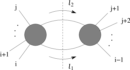
Figure 12: Unitarity cut in the $P_{ij}^{2}-$channel. The blobs represent tree-level amplitudes in which the propagator lines are interpreted as external on-shell particles.

(3) Use reduction techniques to write the integrand of (195) as a sum of terms that contain a constant coefficient times two propagators. Once this is achieved, it is easy to construct a function of scalar box integrals with given coefficients that has such a cut. Then repeat this for all other cuts, remembering that a given scalar box integral has cuts in several different channels. This means that one should not just add the functions obtained from the study of each channel. Instead one has to combine them while avoiding to overcount. Once a function with all the correct discontinuities has been constructed, this must be the final answer for the amplitude. The reason is that supersymmetric amplitudes are four-dimensional cut-constructible, as mentioned above.

Using this technique, all MHV amplitudes and the six-gluon NMHV amplitudes were computed more than ten years ago. More recently, the seven-gluon NMHV amplitude with all minus helicity gluons adjacent was computed by using a combination of this method and the holomorphic anomaly of unitarity cuts [37] in [34, 28]. The same result as well as all other helicity configurations for the seven-gluon amplitude were obtained by the unitarity-based method in [18].

At this point it is important to mention that the integrand in the cut integral (195) is complicated because in general there are many scalar box integrals sharing the same branch cut. The reduction techniques, though systematic, can lead to very large expressions for the scalar box coefficients [18]. These large expressions can be shown to be equivalent to simple formulas obtained as educated guesses [18]. This is a hint that there must be a more direct method for computing such coefficients.

A related difficulty comes from the fact that a given scalar box integral has many different branch cuts. This means that after its coefficient has been computed from a given cut, one still has to disentangle it from other unknown coefficients over and over again in the other cuts. This somehow reduces the efficiency of the method.

One way to improve the situation is by cutting three propagators [18][19]. Note that triple cuts where a single gluon in trapped in between two cut propagators vanish. This would correspond to a cut in a one-particle channel. In the next part of this lecture we will reconsider this issue.

Note that the number of scalar boxes with a given triple cut is less than that with a given unitarity cut. However, in general one still has to apply reduction techniques. A class of amplitudes for which triple cuts are very suitable are next-to-MHV (NMHV) amplitudes [19]. But, one might expect that this procedure becomes cumbersome already for NNMHV amplitudes.

It turns out that there is a way of avoiding the reduction techniques as well as the recalculation of known coefficients. This is achieved by considering quadruple cuts [29] which we now discuss.

8.2.2 Quadruple Cuts

Consider a scalar one-loop Feynman integral, $I$. The integral $I$ is a function of the kinematical invariants constructed out of the external momenta. In general, $I$ is a complicated multi-valued function with branch cuts that are like domain walls in the space of kinematical invariants, $\Sigma$. As it is well known, cutting two propagators in the loop computes the imaginary part of the integral in a certain region of $\Sigma$. This imaginary part of $I$ can be thought of as the discontinuity of $I$ across the branch cut of interest.

Now consider unitarity cuts in several possible channels. One can ask what is the discontinuity across the intersection of two or more cuts. The answer is given by the union of the set of cut propagators! Of particular interest to us is the meaning of cutting all propagators in a one-loop integral; such a cut integral computes the discontinuity across the singularity of highest codimension, which is known as the leading singularity. For a more extensive discussion and references see [42].

As mentioned above, ${\cal N}=4$ one-loop amplitudes of gluons can be written as a linear combination of scalar box integrals with rational coefficients. The scalar box integrals can be thought of as a “basis of vectors” in some sort of vector space. The idea is that this basis is in some appropriate sense orthogonal (In less supersymmetric theories there also are bubble and triangle integrals which break the orthogonality condition).

The one-loop amplitude ${\cal A}_{n}^{\rm 1-loop}$ can now be interpreted as a general vector which can be written as a linear combination of the basis. All we need is the appropriate way of projecting the “vector” ${\cal A}_{n}^{\rm 1-loop}$ onto a given vector $I$ in order to compute the corresponding coefficient.

From our discussion, it is clear that the natural way of doing this is to consider ${\cal A}_{n}^{\rm 1-loop}$ in the region near the leading singularity of $I$, which is unique to $I$. The discontinuity of ${\cal A}_{n}^{\rm 1-loop}$ across such a singularity is the coefficient of $I$, up to a normalization, which is the analog of the norm of $I$.

Let us see how this works in practice. Recall that the scalar box integral (194) is,

$$I_{(K_{1},K_{2},K_{3})}=\int d^{4}\ell{1\over(\ell^{2}+i\epsilon)((\ell-K_{1})^{2}+i\epsilon)((\ell-K_{1}-K_{2})^{2}+i\epsilon)((\ell+K_{4})^{2}+i\epsilon)}.$$ (197)

In the expansion of ${\cal A}^{\rm 1-loop}_{n}$, each $K_{i}$ in (197) is the sum of the momenta of consecutive external gluons.

The discontinuity across the leading singularity $\Delta_{LS}$ is computed by cutting all four propagators. This is called a quadruple cut:

$$\Delta_{LS}I_{(K_{1},K_{2},K_{3})}=\int d^{4}\ell~{}\delta^{(+)}(\ell^{2})~{}\delta^{(+)}((\ell-K_{1})^{2})~{}\delta^{(+)}((\ell-K_{1}-K_{2})^{2})~{}\delta^{(+)}((\ell+K_{4})^{2}).$$ (198)

In order to make the discussion more explicit we introduce notation for the coefficients of $I$ in the expansion of ${\cal A}_{n}^{\rm 1-loop}$ as follows:

$${\cal A}_{n}^{\rm 1-loop}=\sum_{1<i<j<k<m<n}B_{ijkm}I_{(p_{i+1}+\ldots+p_{j},p_{j+1}+\ldots+p_{k},p_{k+1}+\ldots+p_{m})},$$ (199)

where the coefficients $B_{ijkm}$ are rational functions of the spinor products, as mentioned above.

Figure 13: A quadruple cut diagram. Momenta in the cut propagators flows clockwise and external momenta are taken outgoing. The tree-level amplitude ${\cal A}^{\rm tree}_{1}$, for example, has external momenta $(-\ell_{1},i+1,...,j,\ell_{2})$.

By cutting four given propagators in all possible Feynman diagrams contributing to ${\cal A}_{n}^{\rm 1-loop}$ one finds the product of four tree-level amplitudes integrated over the Lorentz invariant phase space of four null vectors.

Comparing the two sides of (199) we find

$$\int d\mu{\cal A}^{\rm tree}_{1}{\cal A}^{\rm tree}_{2}{\cal A}^{\rm tree}_{3}{\cal A}^{\rm tree}_{4}=B_{ijkm}\int d^{4}\ell~{}\delta^{(+)}(\ell^{2})~{}\delta^{(+)}((\ell-K_{1})^{2})~{}\delta^{(+)}((\ell-K_{1}-K_{2})^{2})~{}\delta^{(+)}((\ell+K_{4})^{2})$$ (200)

where the measure is the same one both sides of the integrals,

$$d\mu=d^{4}\ell~{}\delta^{(+)}(\ell^{2})~{}\delta^{(+)}((\ell-K_{1})^{2})~{}\delta^{(+)}((\ell-K_{1}-K_{2})^{2})~{}\delta^{(+)}((\ell+K_{4})^{2}),$$ (201)

and the tree-level amplitudes are defined as follows (see figure (13))

$$\begin{array}[]{rlrl}{\cal A}_{1}^{\rm tree}=&{\cal A}(-\ell_{1},i+1,i+2,\ldots,j-1,j,\ell_{2}),&\quad{\cal A}_{2}^{\rm tree}=&{\cal A}(-\ell_{2},j+1,j+2,\ldots,k-1,k,\ell_{3}),\\ {\cal A}_{3}^{\rm tree}=&{\cal A}(-\ell_{3},k+1,k+2,\ldots,m-1,m,\ell_{4}),&\quad{\cal A}_{4}^{\rm tree}=&{\cal A}(-\ell_{4},m+1,m+2,\ldots,i-1,i,\ell_{1}).\end{array}$$ (202)

In general one might expect that four delta functions localize the integral producing a Jacobian which is common to both sides of (200) and cancels out to give

$$B_{ijkl}={1\over|{\cal S}|}\sum_{\cal S}{\cal A}^{\rm tree}_{1}{\cal A}^{\rm tree}_{2}{\cal A}^{\rm tree}_{3}{\cal A}^{\rm tree}_{4}.$$ (203)

Here ${\cal S}$ is the set of solutions to the conditions imposed by the delta functions, and $|{\cal S}|$ is the number of solutions.

The derivation of the formula for the coefficients (203) assumes that the Jacobian is a smooth function and that it does not vanish for generic momenta of the external gluons and that it is the same for all solutions ${\cal S}$ [28].

It turns out that both assumptions are not valid if at least one of the momenta $K_{i}$ in the box integral is null, i.e., if $K_{i}^{2}=0$ for some $i$. This is where the problem of defining a cut in a one-particle channel, which we mentioned in the discussion of triple cuts, comes back again.

It is not difficult to see that by using $\delta^{(+)}(\ell^{2})$ to reduce the integration over arbitrary $\ell$’s to those lying in the future light-cone and by using that, say, $K_{1}^{2}=0$ one finds that two of the three remaining delta functions are enough to localize the integral. The last delta function, that can be thought of as part of the Jacobian, imposes an extra constraint on the external momenta beyond momentum conservation. Therefore, this makes our two assumptions fail.

This problem of defining a cut in a one-particle channel is the familiar statement that a gluon cannot decay into two gluons. In other words, the tree-level amplitude ${\cal A}_{1}^{\rm tree}$ in (200) vanishes.

It turns out that the way out of both problems is the same. Consider a Wick rotation of (200) in to $--++$ signature. In this case one needs all four delta functions in order to localize the integral. The integration can be done and produces a smooth and generically nonzero Jacobian. The reason for this will be clear shortly.

It remains to see what happens to ${\cal A}_{1}^{\rm tree}$. If it is still zero it would imply that all coefficients with $K_{1}^{2}=0$ are zero. This is known to be false in MHV and NMHV amplitudes.

Let us look more closely at the tree-level amplitude ${\cal A}_{1}$ and the delta function containing only $K_{1}$. There are two cases,

$${\cal A}_{1}(K_{1}^{+},\ell^{+},(\ell-K_{1})^{-}) = {[K_{1},~{}\ell]^{3}\over[K_{1},~{}\ell-K_{1}][\ell-K_{1},~{}\ell]},$$ (204)

$${\cal A}_{2}(K_{1}^{-},\ell^{-},(\ell-K_{1})^{+}) = {\langle{K_{1},~{}\ell}\rangle^{3}\over\langle{K_{1},~{}\ell-K_{1}}\rangle\langle{\ell-K_{1},~{}\ell}\rangle}.$$ (205)

The delta function is given by $\delta((\ell-K_{1})^{2})$. This implies that $\langle{\ell,~{}K_{1}}\rangle[\ell,~{}K_{1}]=0$. As reviewed in section 2, in Minkowski space with real momenta $\lambda$ and $\tilde{\lambda}$ are complex but not independent, i.e., $\tilde{\lambda}=\pm\overline{\lambda}$ and therefore the only solution is $\langle{\ell,~{}K_{1}}\rangle=[\ell,~{}K_{1}]=0$. On the other hand, in $--++$ signature, $\lambda$ and $\tilde{\lambda}$ are real and independent, therefore we can have $\langle{\ell,~{}K_{1}}\rangle=0$ while $[\ell,~{}K_{1}]\neq 0$ or vice versa. This is also the reason why four delta functions are required to localize the integral (198).

This explains how the problem is completely solved. When summing over the set of solutions ${\cal S}$, one must take into account the two possibilities, $\langle{\ell,~{}K_{1}}\rangle=0$ or $[\ell,~{}K_{1}]=0$. One of them makes ${\cal A}_{1}^{\rm tree}$ vanish while the other does not. Actually, the presence of two solutions is important even in the case when no $K_{i}$ is a null vector. The reason is that each solution produces a function with a square root. However, the coefficient must be a rational function. The resolution to this little puzzle is that by adding the two solutions, which differ only in the branch the square root takes, one always produces a rational function.

One can easily see that in general there are only two solutions to the delta function constraints. The two solutions can be found explicitly in full generality; we refer the reader to [28] for the actual formula. This implies that $|{\cal S}|=2$. Using this in (203) we find a formula for all one-loop ${\cal N}=4$ amplitude coefficients in terms of tree-level amplitudes,

$$B_{ijkl}={1\over 2}\sum_{h,\cal S}{\cal A}^{\rm tree}_{1}{\cal A}^{\rm tree}_{2}{\cal A}^{\rm tree}_{3}{\cal A}^{\rm tree}_{4}.$$ (206)

The sum on the right hand side of (206) is over the two solutions ${\cal S}$ and over all internal particles in the ${\cal N}=4$ supermultiplet.

8.2.3 Examples

As a simple example consider the coefficient of $I_{(3+4,5+6,7+1)}$ in ${\cal A}(1^{-},2^{-},3^{-},4^{+},5^{+},6^{+},7^{+})$.

In this case, only one internal helicity configuration gives a non zero contribution and it allows only gluons to run in the loop.

Figure 14: $(a)$ Scalar Box Integral $I_{3+4,5+6,7+1}$. $(b)$ Quadruple cut diagram of ${\cal A}_{7}^{\rm 1-loop}$ corresponding to $I_{3+4,5+6,7+1}$. Blobs represent tree-level amplitudes.

Using (206) we find

$$B_{3572}=\frac{1}{2}{[\ell_{1}~{}\ell_{4}]^{3}\over[\ell_{1}~{}2][2~{}\ell_{4}]}{[4~{}\ell_{2}]^{3}\over[\ell_{2}~{}\ell_{1}][\ell_{1}~{}3][3~{}4]}{[5~{}6]^{3}\over[6~{}\ell_{3}][\ell_{3}~{}\ell_{2}][\ell_{2}~{}5]}{[\ell_{3}~{}7]^{3}\over[7~{}1][1~{}\ell_{4}][\ell_{4}~{}\ell_{3}]}$$ (207)

After solving the equations for $\ell_{i}$ and plugging in the answer in (207) one finds a simple expression for $B_{3572}$ [28, 18]

$$-{\langle{1~{}2}\rangle^{3}\langle{2~{}3}\rangle^{3}[5~{}6]^{3}\over\langle{7~{}1}\rangle\langle{3~{}4}\rangle\langle 2|3+4|5]\langle 2|7+1|6](\langle{7~{}1}\rangle\langle 2|3+4|1]-t_{2}^{[3]}\langle{7~{}2}\rangle)(t_{7}^{[2]}\langle{2~{}4}\rangle-\langle{3~{}4}\rangle\langle 2|7+1|3])}.$$ (208)

Acknowledgements

It is pleasure to thank R. Britto, B. Feng for proof-reading parts of the manuscript and especially to E. Witten for giving us a permission to base sections 2-4 of the lecture notes on his lectures given at PITP, IAS Summer 2004. Work of F. Cachazo was supported in part by the Martin A. and Helen Chooljian Membership at the Institute for Advanced Study and by DOE grant DE-FG02-90ER40542 and that of P. Svrček in part by Princeton University Centennial Fellowship and by NSF grants PHY-9802484 and PHY-0243680. Opinions and conclusions expressed here are those of the authors and do not necessarily reflect the views of funding agencies.

References

- [1] Y. Abe, V. P. Nair and M. I. Park, “Multigluon amplitudes, N = 4 constraints and the WZW model,” Phys. Rev. D 71, 025002 (2005) [arXiv:hep-th/0408191].
- [2] Y. Abe, “An interpretation of multigraviton amplitudes,” arXiv:hep-th/0504174.
- [3] M. Aganagic and C. Vafa, “Mirror symmetry and supermanifolds,” arXiv:hep-th/0403192.
- [4] M. F. Atiyah, Geometry Of Yang-Mills Fields, Lezioni Fermiane (Academia Nazionale dei Lincei and Scuola Normale Superiore, Pisa, 1979).
- [5] S. D. Badger, E. W. N. Glover and V. V. Khoze, “MHV rules for Higgs plus multi-parton amplitudes,” JHEP 0503, 023 (2005) [arXiv:hep-th/0412275].
- [6] S. D. Badger, E. W. N. Glover, V. V. Khoze and P. Svrcek, “Recursion relations for gauge theory amplitudes with massive particles,” arXiv:hep-th/0504159.
- [7] I. Bars, “Twistor superstring in 2T-physics,” Phys. Rev. D 70, 104022 (2004) [arXiv:hep-th/0407239].
- [8] J. Bedford, A. Brandhuber, B. Spence and G. Travaglini, “Non-supersymmetric loop amplitudes and MHV vertices,” arXiv:hep-th/0412108.
- [9] J. Bedford, A. Brandhuber, B. Spence and G. Travaglini, “A twistor approach to one-loop amplitudes in N = 1 supersymmetric Yang-Mills theory,” Nucl. Phys. B 706, 100 (2005) [arXiv:hep-th/0410280].
- [10] J. Bedford, A. Brandhuber, B. Spence and G. Travaglini, “A recursion relation for gravity amplitudes,” arXiv:hep-th/0502146.
- [11] I. Bena, Z. Bern and D. A. Kosower, “Twistor-space recursive formulation of gauge theory amplitudes,” Phys. Rev. D 71, 045008 (2005) [arXiv:hep-th/0406133].
- [12] I. Bena, Z. Bern, D. A. Kosower and R. Roiban, “Loops in twistor space,” [arXiv:hep-th/0410054].
- [13] F. A. Berends and W. T. Giele, “Recursive Calculations For Processes With N Gluons,” Nucl. Phys. B 306, 759 (1988).
- [14] F. A. Berends, W. T. Giele and H. Kuijf, “Exact And Approximate Expressions For Multi - Gluon Scattering,” Nucl. Phys. B 333, 120 (1990).
- [15] N. Berkovits, “An alternative string theory in twistor space for N = 4 super-Yang-Mills,” Phys. Rev. Lett. 93, 011601 (2004) [arXiv:hep-th/0402045].
- [16] N. Berkovits and E. Witten, “Conformal supergravity in twistor-string theory,” JHEP 0408, 009 (2004) [arXiv:hep-th/0406051].
- [17] N. Berkovits and L. Motl, “Cubic twistorial string field theory,” JHEP 0404, 056 (2004) [arXiv:hep-th/0403187].
- [18] Z. Bern, V. Del Duca, L. J. Dixon and D. A. Kosower, “All non-maximally-helicity-violating one-loop seven-gluon amplitudes in N = 4 super-Yang-Mills theory,” Phys. Rev. D 71, 045006 (2005) [arXiv:hep-th/0410224].
- [19] Z. Bern, L. J. Dixon and D. A. Kosower, “All next-to-maximally helicity-violating one-loop gluon amplitudes in N = 4 super-Yang-Mills theory,” arXiv:hep-th/0412210.
- [20] Z. Bern, D. Forde, D. A. Kosower and P. Mastrolia, “Twistor-inspired construction of electroweak vector boson currents,” arXiv:hep-ph/0412167.
- [21] Z. Bern, L. J. Dixon and D. A. Kosower, “On-shell recurrence relations for one-loop QCD amplitudes,” arXiv:hep-th/0501240.
- [22] Z. Bern, N. E. J. Bjerrum-Bohr and D. C. Dunbar, “Inherited twistor-space structure of gravity loop amplitudes,” arXiv:hep-th/0501137.
- [23] Z. Bern, L. J. Dixon, D. C. Dunbar and D. A. Kosower, “One loop n point gauge theory amplitudes, unitarity and collinear limits,” Nucl. Phys. B 425, 217 (1994) [arXiv:hep-ph/9403226].
- [24] Z. Bern, L. J. Dixon, D. C. Dunbar and D. A. Kosower, “Fusing gauge theory tree amplitudes into loop amplitudes,” Nucl. Phys. B 435, 59 (1995) [arXiv:hep-ph/9409265].
- [25] T. G. Birthwright, E. W. N. Glover, V. V. Khoze and P. Marquard, “Multi-gluon collinear limits from MHV diagrams,” arXiv:hep-ph/0503063.
- [26] N. E. J. Bjerrum-Bohr, D. C. Dunbar and H. Ita, “Six-point one-loop N = 8 supergravity NMHV amplitudes and their IR arXiv:hep-th/0503102.
- [27] A. Brandhuber, B. Spence and G. Travaglini, “One-loop gauge theory amplitudes in N = 4 super Yang-Mills from MHV vertices,” Nucl. Phys. B 706, 150 (2005) [arXiv:hep-th/0407214].
- [28] R. Britto, F. Cachazo and B. Feng, “Computing one-loop amplitudes from the holomorphic anomaly of unitarity cuts,” Phys. Rev. D 71, 025012 (2005) [arXiv:hep-th/0410179].
- [29] R. Britto, F. Cachazo and B. Feng, “Generalized unitarity and one-loop amplitudes in N = 4 super-Yang-Mills,” arXiv:hep-th/0412103.
- [30] R. Britto, F. Cachazo and B. Feng, “New recursion relations for tree amplitudes of gluons,” arXiv:hep-th/0412308.
- [31] R. Britto, B. Feng, R. Roiban, M. Spradlin and A. Volovich, “All split helicity tree-level gluon amplitudes,” arXiv:hep-th/0503198.
- [32] R. Britto, F. Cachazo, B. Feng and E. Witten, “Direct proof of tree-level recursion relation in Yang-Mills theory,” arXiv:hep-th/0501052.
- [33] R. Britto, E. Buchbinder, F. Cachazo and B. Feng, “One-loop amplitudes of gluons in SQCD,” arXiv:hep-ph/0503132.
- [34] F. Cachazo, “Holomorphic anomaly of unitarity cuts and one-loop gauge theory amplitudes,” arXiv:hep-th/0410077.
- [35] F. Cachazo, P. Svrcek and E. Witten, “MHV vertices and tree amplitudes in gauge theory,” JHEP 0409, 006 (2004) [arXiv:hep-th/0403047].
- [36] F. Cachazo, P. Svrcek and E. Witten, “Twistor space structure of one-loop amplitudes in gauge theory,” JHEP 0410, 074 (2004) [arXiv:hep-th/0406177].
- [37] F. Cachazo, P. Svrcek and E. Witten, “Gauge theory amplitudes in twistor space and holomorphic anomaly,” JHEP 0410, 077 (2004) [arXiv:hep-th/0409245].
- [38] F. Cachazo and P. Svrcek, “Tree level recursion relations in general relativity,” arXiv:hep-th/0502160.
- [39] S. Catani, “The singular behaviour of QCD amplitudes at two-loop order,” Phys. Lett. B 427, 161 (1998) [arXiv:hep-ph/9802439].
- [40] D. W. Chiou, O. J. Ganor, Y. P. Hong, B. S. Kim and I. Mitra, “Massless and massive three dimensional super Yang-Mills theory and arXiv:hep-th/0502076.
- [41] L. J. Dixon, “Calculating scattering amplitudes efficiently,” arXiv:hep-ph/9601359.
- [42] R. J. Eden, P. V. Landshoff, D. I. Olive and J. C. Polkinghorne, The Analytic S-Matrix, Cambridge University Press, 1966.
- [43] S. Gukov, L. Motl and A. Neitzke, “Equivalence of twistor prescriptions for super Yang-Mills,” arXiv:hep-th/0404085.
- [44] B. S. DeWitt, “Quantum Theory Of Gravity. Iii. Applications Of The Covariant Theory,” Phys. Rev. 162 (1967) 1239.
- [45] L. J. Dixon, E. W. N. Glover and V. V. Khoze, “MHV rules for Higgs plus multi-gluon amplitudes,” JHEP 0412, 015 (2004) [arXiv:hep-th/0411092].
- [46] G. Georgiou and V. V. Khoze, “Tree amplitudes in gauge theory as scalar MHV diagrams,” JHEP 0405, 070 (2004) [arXiv:hep-th/0404072].
- [47] G. Georgiou, E. W. N. Glover and V. V. Khoze, “Non-MHV tree amplitudes in gauge theory,” JHEP 0407, 048 (2004) [arXiv:hep-th/0407027].
- [48] S. Giombi, R. Ricci, D. Robles-Llana and D. Trancanelli, “A note on twistor gravity amplitudes,” JHEP 0407, 059 (2004) [arXiv:hep-th/0405086].
- [49] S. Giombi, M. Kulaxizi, R. Ricci, D. Robles-Llana, D. Trancanelli and K. Zoubos, “Orbifolding the twistor string,” arXiv:hep-th/0411171.
- [50] L.D. Landau, Nucl. Phys. 13, 181 (1959); S. Mandelstam, Phys. Rev. 112, 1344 (1958), 115, 1741 (1959); R.E. Cutskosky, J. Math. Phys. 1, 429 (1960).
- [51] G. ’t Hooft, “A Planar Diagram Theory For Strong Interactions,” Nucl. Phys. B 72, 461 (1974).
- [52] S. A. Huggett and K. P. Tod, “An Introduction To Twistor Theory,”
- [53] M. x. Luo and C. k. Wen, “One-loop maximal helicity violating amplitudes in N = 4 super Yang-Mills theories,” JHEP 0411, 004 (2004) [arXiv:hep-th/0410045].
- [54] M. x. Luo and C. k. Wen, “Systematics of one-loop scattering amplitudes in N = 4 super Yang-Mills theories,” Phys. Lett. B 609, 86 (2005) [arXiv:hep-th/0410118].
- [55] M. x. Luo and C. k. Wen, “Recursion relations for tree amplitudes in super gauge theories,” arXiv:hep-th/0501121.
- [56] M. x. Luo and C. k. Wen, “Compact formulas for all tree amplitudes of six partons,” arXiv:hep-th/0502009.
- [57] V. V. Khoze, “Gauge theory amplitudes, scalar graphs and twistor space,” arXiv:hep-th/0408233.
- [58] D. A. Kosower, “Next-to-maximal helicity violating amplitudes in gauge theory,” Phys. Rev. D 71, 045007 (2005) [arXiv:hep-th/0406175].
- [59] M. Kulaxizi and K. Zoubos, “Marginal deformations of N = 4 SYM from open / closed twistor strings,” arXiv:hep-th/0410122.
- [60] J. M. Maldacena, “The large N limit of superconformal field theories and supergravity,” Adv. Theor. Math. Phys. 2, 231 (1998) [Int. J. Theor. Phys. 38, 1113 (1999)] [arXiv:hep-th/9711200].
- [61] M. L. Mangano, S. J. Parke and Z. Xu, “Duality And Multi - Gluon Scattering,” Nucl. Phys. B 298, 653 (1988).
- [62] M. L. Mangano and S. J. Parke, “Multiparton Amplitudes In Gauge Theories,” Phys. Rept. 200, 301 (1991).
- [63] V. P. Nair, “A Current Algebra For Some Gauge Theory Amplitudes,” Phys. Lett. B 214 (1988) 215.
- [64] V. P. Nair, “A note on MHV amplitudes for gravitons,” arXiv:hep-th/0501143.
- [65] A. Neitzke and C. Vafa, “N = 2 strings and the twistorial Calabi-Yau,” arXiv:hep-th/0402128.
- [66] J. Park and S. J. Rey, “Supertwistor orbifolds: Gauge theory amplitudes and topological strings,” JHEP 0412, 017 (2004) [arXiv:hep-th/0411123].
- [67] L.M. Brown and R.P. Feynman, Phys. Rev. 85:231 (1952); G. Passarino and M. Veltman, Nucl. Phys. B160:151 (1979); G. ’t Hooft and M. Veltman, Nucl. Phys. B153:365 (1979);R.G. Stuart, Comp. Phys. Comm. 48:367 (1988); R.G. Stuart and A. Gongora, Comp. Phys. Comm. 56:337 (1990).
- [68] R. Penrose, “The Nonlinear Graviton,” Gen. Rel. Grav. 7, 171 (1976).
- [69] C. Quigley and M. Rozali, “One-loop MHV amplitudes in supersymmetric gauge theories,” JHEP 0501, 053 (2005) [arXiv:hep-th/0410278].
- [70] R. Roiban, M. Spradlin and A. Volovich, “A googly amplitude from the B-model in twistor space,” JHEP 0404, 012 (2004) [arXiv:hep-th/0402016].
- [71] R. Roiban, M. Spradlin and A. Volovich, “On the tree-level S-matrix of Yang-Mills theory,” Phys. Rev. D 70, 026009 (2004) [arXiv:hep-th/0403190].
- [72] R. Roiban, M. Spradlin and A. Volovich, “Dissolving N = 4 loop amplitudes into QCD tree amplitudes,” Phys. Rev. Lett. 94, 102002 (2005) [arXiv:hep-th/0412265].
- [73] X. Su and J. B. Wu, “Six-quark amplitudes from fermionic MHV vertices,” arXiv:hep-th/0409228.
- [74] E. Witten, “Mirror manifolds and topological field theory,” arXiv:hep-th/9112056.
- [75] E. Witten, “Chern-Simons gauge theory as a string theory,” Prog. Math. 133, 637 (1995) [arXiv:hep-th/9207094].
- [76] E. Witten, “Perturbative gauge theory as a string theory in twistor space,” Commun. Math. Phys. 252, 189 (2004) [arXiv:hep-th/0312171].
- [77] E. Witten, “Parity invariance for strings in twistor space,” arXiv:hep-th/0403199.
- [78] J. B. Wu and C. J. Zhu, “MHV vertices and scattering amplitudes in gauge theory,” JHEP 0407, 032 (2004) [arXiv:hep-th/0406085].
- [79] J. B. Wu and C. J. Zhu, “MHV vertices and fermionic scattering amplitudes in gauge theory with quarks and gluinos,” JHEP 0409, 063 (2004) [arXiv:hep-th/0406146].
- [80] C. J. Zhu, “The googly amplitudes in gauge theory,” JHEP 0404, 032 (2004) [arXiv:hep-th/0403115].