Wightman function and Casimir densities for Robin plates
in the Fulling–Rindler vacuum

Abstract

Wightman function, the vacuum expectation values of the field square and the energy–momentum tensor are investigated for a massive scalar field with an arbitrary curvature coupling parameter in the region between two infinite parallel plates moving by uniform proper acceleration. We assume that the field is prepared in the Fulling–Rindler vacuum state and satisfies Robin boundary conditions on the plates. The mode–summation method is used with a combination of a variant of the generalized Abel–Plana formula. This allows to extract manifestly the contributions to the expectation values due to a single boundary and to present the second plate-induced parts in terms of exponentially convergent integrals. Various limiting cases are investigated. The vacuum forces acting on the boundaries are presented as a sum of the self–action and ’interaction’ terms. The first one contains well known surface divergences and needs a further renormalization. The ’interaction’ forces between the plates are investigated as functions of the proper accelerations and coefficients in the boundary conditions. We show that there is a region in the space of these parameters in which the ’interaction’ forces are repulsive for small distances and attractive for large distances.

PACS number(s): 03.70.+k, 11.10.Kk, 04.62.+v

1 Introduction

The Casimir effect is one of the most interesting macroscopic manifestations of the nontrivial structure of the vacuum state in quantum field theory (see, e.g., [1, 2, 3, 4] and references therein). The effect is a phenomenon common to all systems characterized by fluctuating quantities and results from changes in the vacuum fluctuations of a quantum field that occur because of the imposition of boundary conditions or the choice of topology. It may have important implications on all scales, from cosmological to subnuclear, and has become in recent decades an increasingly popular topic in quantum field theory. It is well known that the uniqueness of the vacuum state is lost when we work within the framework of quantum field theory in a general curved spacetime or in non–inertial frames. In particular, the use of general coordinate transformations in quantum field theory in flat spacetime leads to an infinite number of unitary inequivalent representations of the commutation relations. Different inequivalent representations will in general give rise to different vacuum states. For instance, the vacuum state for a uniformly accelerated observer, the Fulling–Rindler vacuum [5, 6, 7, 8, 9], turns out to be inequivalent to that for an inertial observer, the familiar Minkowski vacuum. Quantum field theory in accelerated systems contains many special features produced by a gravitational field. In particular, the near horizon geometry of most black holes is well approximated by Rindler spacetime and a better understanding of physical effects in this background could serve as a handle to deal with more complicated geometries like Schwarzschild. The Rindler geometry shares most of the qualitative features of black holes and is simple enough to allow detailed analysis. Another motivation for the investigation of quantum effects in the Rindler space is related to the fact that this space is conformally related to de Sitter space and to Robertson–Walker space with negative spatial curvature. As a result the expectation values of the energy–momentum tensor for conformally invariant fields and for corresponding conformally transformed boundaries on the de Sitter and Robertson–Walker backgrounds can be generated from the corresponding Rindler counterpart by the standard transformation (see, for instance, [10]).

An interesting topic in the investigations of the Casimir effect is the dependence of the vacuum characteristics on the type of the vacuum. Vacuum expectation values of the energy-momentum tensor induced by an infinite plane boundary moving with uniform proper acceleration through the Fulling-Rindler vacuum was studied by Candelas and Deutsch [11] for the conformally coupled $4D$ Dirichlet and Neumann massless scalar and electromagnetic fields. In this paper only the region of the right Rindler wedge to the right of the barrier is considered. In Ref. [12] we have investigated the Wightman function and the vacuum energy-momentum tensor for a massive scalar field with general curvature coupling parameter, satisfying the Robin boundary conditions on the infinite plane in an arbitrary number of spacetime dimensions and for the electromagnetic field. We have considered both regions, including the one between the barrier and Rindler horizon. The vacuum expectation values of the energy-momentum tensor for scalar fields with Dirichlet and Neumann boundary conditions and for the electromagnetic field in the geometry of two parallel plates moving by uniform accelerations are investigated in Ref. [13]. In particular, the vacuum forces acting on the boundaries are evaluated. They are presented as a sum of the ’interaction’ and self-action parts. The ’interaction’ forces between the plates are always attractive for both scalar and electromagnetic cases. Due to the well-known surface divergences in the boundary parts, the total Casimir energy cannot be obtained by direct integration of the vacuum energy density and needs an additional renormalization. In Ref. [14] by using the zeta function technique, the Casimir energy is evaluated for massless scalar fields under Dirichlet and Neumann boundary conditions, and for the electromagnetic field with perfect conductor boundary conditions on one and two parallel plates. On background of manifolds with boundaries, the physical quantities, in general, will receive both volume and surface contributions and the surface terms play an important role in various branches of physics. An expression for the surface energy-momentum tensor for a scalar field with general curvature coupling parameter in the general case of bulk and boundary geometries is derived in Ref. [15]. In Ref. [16] the vacuum expectation value of the surface energy-momentum tensor is evaluated for a massles scalar field obeying Robin boundary condition on an infinite plane moving by uniform proper acceleration. By using the conformal relation between the Rindler and de Sitter spacetimes and the results from [12], in Ref. [17] the vacuum energy-momentum tensor for a scalar field is evaluated in de Sitter spacetime in presence of a curved brane on which the field obeys the Robin boundary condition with coordinate dependent coefficients.

In the present paper the Wightman function and the vacuum expectation value of the field square the energy-momentum tensor are investigated for a massive scalar field with an arbitrary curvature coupling parameter obeying the Robin boundary conditions on two parallel branes moving by uniform proper accelerations through the Fulling-Rindler vacuum. The general case is considered when the constants in the boundary conditions are different for separate plates. Robin type conditions are an extension of Dirichlet and Neumann boundary conditions and appear in a variety of situations, including the considerations of vacuum effects for a confined charged scalar field in external fields [18], spinor and gauge field theories, quantum gravity and supergravity [19, 20]. Robin conditions can be made conformally invariant, while purely-Neumann conditions cannot. Thus, Robin-type conditions are needed when one deals with conformally invariant theories in the presence of boundaries and wishes to preserve this invariance. It is interesting to note that the quantum scalar field satisfying the Robin condition on the boundary of cavity violates the Bekenstein’s entropy-to-energy bound near certain points in the space of the parameter defining the boundary condition [21]. The Robin boundary conditions are an extension of those imposed on perfectly conducting boundaries and may, in some geometries, be useful for depicting the finite penetration of the field into the boundary with the ’skin-depth’ parameter related to the Robin coefficient. Robin boundary conditions naturally arise for scalar and fermion bulk fields in the Randall-Sundrum model [22, 23, 24]. In this model the bulk geometry is a slice of anti-de Sitter space and the corresponding Robin coefficients are related to the curvature scale of the space.

The outline of this paper is the following. In the next section the Wightman function is considered. The corresponding mode-sum is evaluated by using the generalized Abel-Plana summation formula [25]. This allows us to extract from the corresponding vacuum expectation values the Wightman function for the geometry of a single plate and to present the remained part in the form of the exponentially convergent integrals. The vacuum expectation values of the field square and the Casimir energy-momentum tensor is evaluated in Section 3. Various limiting cases are considered. In Section 4 we investigate the vacuum ’interaction’ forces between the plates as functions on corresponding proper accelerations. Section 5 contains a summary of the work and some suggestions for further research. In Appendix A on the base of the generalized Abel-Plana formula, a summation formula is derived for the series over zeros of a combination of the Bessel modified functions with an imaginary order.

2 Wightman function

We consider a real scalar field $\varphi(x)$ with general curvature coupling parameter $\zeta$ satisfying the field equation

$$\left(\nabla_{\mu}\nabla^{\mu}+m^{2}+\zeta R\right)\varphi=0,$$ (2.1)

where $R$ is the scalar curvature for a $(D+1)$–dimensional background spacetime, and $\nabla_{\mu}$ is the covariant derivative operator. For special cases of minimally and conformally coupled scalars one has $\zeta=0$ and $\zeta=(D-1)/4D$, respectively. Our main interest in this paper will be the Wightman function, the vacuum expectation values (VEVs) of the field square and the energy-momentum tensor in the Rindler spacetime induced by two parallel plates moving with uniform proper acceleration when the quantum field is prepared in the Fulling-Rindler vacuum. For this problem the background spacetime is flat and in Eq. (2.1) we have $R=0$. As a result the eigenmodes are independent on the curvature coupling parameter. However, the local characteristics of the vacuum such as energy density and vacuum stresses  depend on this parameter.

In the accelerated frame it is convenient to introduce Rindler coordinates $(\tau,\xi,\mathbf{x})$ related to the Minkowski ones, $(t,x^{1},\mathbf{x})$ by formulas

$$t=\xi\sinh\tau,\quad x^{1}=\xi\cosh\tau,$$ (2.2)

where $\mathbf{x}=(x^{2},\ldots,x^{D})$ denotes the set of coordinates parallel to the plates. In these coordinates the Minkowski line element takes the form

$$ds^{2}=\xi^{2}d\tau^{2}-d\xi^{2}-d\mathbf{x}^{2},$$ (2.3)

and a world line defined by $\xi,\mathbf{x}=\mathrm{const}$ describes an observer with constant proper acceleration $\xi^{-1}$. The Rindler time coordinate $\tau$ is proportional to the proper time along a family of uniformly accelerated trajectories which fill the Rindler wedge, with the proportionality constant equal to the acceleration. Assuming that the plates are situated in the right Rindler wedge $x^{1}>\left|t\right|$, we will let the surfaces $\xi=a$ and $\xi=b$, $b>a$ represent the trajectories of these boundaries, which therefore have proper accelerations $a^{-1}$ and $b^{-1}$ (see Fig. 1). We will consider the case of a scalar field satisfying Robin boundary conditions on the surfaces of the plates:

$$\left.\left(A_{j}+B_{j}\frac{\partial}{\partial\xi}\right)\varphi\right|_{\xi=j}=0,\quad j=a,b,$$ (2.4)

with constant coefficients $A_{j}$ and $B_{j}$. Dirichlet and Neumann boundary conditions are obtained from here as special cases. All results below will depend, of course, on the ratios $A_{j}/B_{j}$ only. However, to keep the transition to Dirichlet and Neumann cases transparent, we write the boundary conditions in the form (2.4).

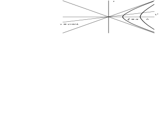
Figure 1: The $(x^{1},t)$ plane with the Rindler coordinates. The heavy lines $\xi=a$ and $\xi=b$ represent the trajectories of the plates.

The plates divide the right Rindler wedge into three regions: $0<\xi<a$, $\xi>b$, and $a<\xi<b$. The VEVs in two first regions are the same as those induced by single plates located at $\xi=a$ and $\xi=b$, respectively. As these VEVs are investigated in Ref. [12], in the consideration below we restrict ourselves to the region between the plates. First we consider the positive frequency Wightman function $G^{+}(x,x^{\prime})=\left\langle 0\left|\varphi(x)\varphi(x^{\prime})\right|0\right\rangle$, with $\left.|0\right\rangle$ being the amplitude for the corresponding vacuum state. The VEVs of the field square and the energy-momentum tensor can be evaluated on the base of this function. In addition, the Wightman function determines the response of the particle detector of Unruh-DeWitt type, moving through the vacuum under consideration. By expanding the field operator over the complete set of eigenfunctions $\left\{\varphi_{\alpha}(x),\varphi_{\alpha}^{\ast}(x)\right\}$ satisfying boundary conditions (2.4) and using the commutation relations one finds

$$G^{+}(x,x^{\prime})=\sum_{\alpha}\varphi_{\alpha}(x)\varphi_{\alpha}^{\ast}(x^{\prime}),$$ (2.5)

where the collective index $\alpha$ is a set of quantum numbers specifying the solution.

To evaluate the mode sum in formula (2.5) we need the form of the eigenfunctions $\varphi_{\alpha}(x)$ (for a recent discussion of eigenmodes in four Rindler sectors and relations between them see, for instance, [26]). For the geometry under consideration the metric and boundary conditions are static and translational invariant in the hyperplane parallel to the plates. It follows from here that the corresponding part of the eigenfunctions can be taken in the standard plane wave form:

$$\varphi_{\alpha}=C\phi(\xi)\exp\left[i\left(\mathbf{kx}-\omega\tau\right)\right],\quad\alpha=(\mathbf{k},\omega),$$ (2.6)

with the wave vector $\mathbf{k}=(k_{2},\ldots,k_{D})$. The frequency $\omega$ in Eq. (2.6) corresponds to the dimensionless coordinate $\tau$ and hence is dimensionless. The proper time $\tau_{g}$ and the frequency $\omega_{g}$ measured by a uniformly accelerated observer with the proper acceleration $g$ and world line $(x^{1})^{2}-t^{2}=g^{-2}$ are related to $\tau$ and $\omega$ by the formulas $\tau_{g}=\tau/g$, $\omega_{g}=\omega g$ (the features of the measurements for time, frequency, and length relative to a Rindler frame as compared to a Minkowski frame are discussed in Ref. [27]). The equation for $\phi(\xi)$ is obtained from field equation (2.1) on background of metric (2.3) and has the form

$$\xi^{2}\phi^{\prime\prime}(\xi)+\xi\phi^{\prime}(\xi)+\left(\omega^{2}-\lambda^{2}\xi^{2}\right)\phi(\xi)=0,$$ (2.7)

where the prime denotes a differentiation with respect to the argument of the function,

$$\lambda=\sqrt{k^{2}+m^{2}},$$ (2.8)

and $k=|\mathbf{k}|$. In the region between the plates the linearly independent solutions to equation (2.7) are the Bessel modified functions $I_{i\omega}(k\xi)$ and $K_{i\omega}(k\xi)$. The solution satisfying boundary condition (2.4) on the plate $\xi=b$ has the form

$$Z_{i\omega}^{(b)}(\lambda\xi,\lambda b)=\bar{I}_{i\omega}^{(b)}(\lambda b)K_{i\omega}(\lambda\xi)-\bar{K}_{i\omega}^{(b)}(\lambda b)I_{i\omega}(\lambda\xi).$$ (2.9)

Here and below for a given function $f(z)$ we use the notations

$$\bar{f}^{(j)}(z)=A_{j}f(z)+\frac{B_{j}}{j}zf^{\prime}(z),\quad j=a,b.$$ (2.10)

Note that function (2.9) is real, $Z_{i\omega}^{(b)}(\lambda\xi,\lambda b)=Z_{-i\omega}^{(b)}(\lambda\xi,\lambda b)$. From the boundary condition on the plate $\xi=a$ we find that the possible values for $\omega$ are roots to the equation

$$Z_{i\omega}(\lambda a,\lambda b)=0,$$ (2.11)

with the notation

$$Z_{\omega}(u,v)=\bar{I}_{\omega}^{(b)}(v)\bar{K}_{\omega}^{(a)}(u)-\bar{K}_{\omega}^{(b)}(v)\bar{I}_{\omega}^{(a)}(u).$$ (2.12)

For a fixed $\lambda$, the equation (2.11) has an infinite set of real solutions with respect to $\omega$. We will denote them by $\omega_{n}=\omega_{n}(\lambda a,\lambda b)$, $\omega_{n}>0$, $n=1,2,\ldots$, and will assume that they are arranged in the ascending order $\omega_{n}<\omega_{n+1}$. In addition to the real zeros, in dependence of the values of the ratios $A_{j}/B_{j}$, equation (2.11) can have a finite set of purely imaginary solutions. The presence of such solutions leads to the modes with an imaginary frequency and, hence, to the unstable vacuum. In the consideration below we will assume the values of the coefficients in Eq. (2.4) for which the imaginary solutions are absent and the vacuum is stable.

The coefficient $C$ in formula (2.6) is determined from the standard Klein-Gordon orthonormality condition for the eigenfunctions which for metric (2.3) takes the form

$$\int d\mathbf{x}\int_{a}^{b}\frac{d\xi}{\xi}\varphi_{\alpha}\overleftrightarrow{\partial}_{\tau}\varphi_{\alpha^{\prime}}^{\ast}=i\delta_{\alpha\alpha^{\prime}}.$$ (2.13)

The $\xi$-integral on the left of this formula is evaluated using the integration formula

$$\int_{a}^{b}\frac{d\xi}{\xi}\phi_{1\omega}(\xi)\phi_{2v}(\xi)=\xi\left.\frac{\phi_{1\omega}(\xi)\phi_{2\upsilon}^{\prime}(\xi)-\phi_{2\nu}(\xi)\phi_{1\omega}^{\prime}(\xi)}{\omega^{2}-\upsilon^{2}}\right|_{a}^{b},$$ (2.14)

valid for any two solutions $\phi_{l\omega}(\xi)$, $l=1,2$, to equation (2.7). Taking into account boundary condition (2.4), from Eq. (2.13) for the normalization coefficient one finds

$$C^{2}=\left.\frac{\left(2\pi\right)^{1-D}\bar{I}_{i\omega}^{(a)}(\lambda a)}{\bar{I}_{i\omega}^{(b)}(\lambda b)\frac{\partial}{\partial\omega}Z_{i\omega}(\lambda a,\lambda b)}\right|_{\omega=\omega_{n}}.$$ (2.15)

Now substituting the eigenfunctions

$$\varphi_{\alpha}(x)=CZ_{i\omega_{n}}^{(b)}(\lambda\xi,\lambda b)\exp\left[i\left(\mathbf{kx}-\omega_{n}\tau\right)\right]$$ (2.16)

into the mode sum formula (2.5), for the positive frequency Wightman function one finds

$$G^{+}(x,x^{\prime}) = \int\frac{d\mathbf{k}e^{i\mathbf{k}(\mathbf{x}-\mathbf{x}^{\prime})}}{(2\pi)^{D-1}}\sum_{n=1}^{\infty}\frac{\bar{I}_{i\omega}^{(a)}(\lambda a)e^{-i\omega(\tau-\tau^{\prime})}}{\bar{I}_{i\omega}^{(b)}(\lambda b)\frac{\partial}{\partial\omega}Z_{i\omega}(\lambda a,\lambda b)}$$ (2.17)

$$\times\left.Z_{i\omega}^{(b)}(\lambda\xi,\lambda b)Z_{i\omega}^{(b)}(\lambda\xi^{\prime},\lambda b)\right|_{\omega=\omega_{n}}.$$

As the expressions for the eigenfrequencies $\omega_{n}$ (as functions on $\lambda a$, $\lambda b$, $A_{j}/B_{j}$) are not explicitly known, the form (2.17) of the Wightman function is inconvenient. For the further evoluation of this VEV we can apply to the sum over $n$ the summation formula (A.4) derived in Appendix A on the base of the generalized Abel-Plana formula. As a function $F(z)$ in formula (A.4) let us choose

$$F(z)=\frac{Z_{iz}^{(b)}(\lambda\xi,\lambda b)Z_{iz}^{(b)}(\lambda\xi^{\prime},\lambda b)}{\bar{I}_{iz}^{(b)}(\lambda b)\bar{I}_{-iz}^{(b)}(\lambda b)}e^{-iz(\tau-\tau^{\prime})}.$$ (2.18)

Condition (A.5) for this function is satisfied if $a^{2}e^{|\tau-\tau^{\prime}|}<\xi\xi^{\prime}$. In particular, this is the case in the coincidence limit $\tau=\tau^{\prime}$ in the region under consideration: $\xi,\xi^{\prime}>a$. By using formula (A.4), for the Wightman function one obtains the expression

$$G^{+}(x,x^{\prime}) = G^{+}(x,x^{\prime};b)-\int\frac{d\mathbf{k\,}e^{i\mathbf{k}(\mathbf{x}-\mathbf{x}^{\prime})}}{\pi(2\pi)^{D-1}}\int_{0}^{\infty}d\omega\,\Omega_{b\omega}(\lambda a,\lambda b)$$ (2.19)

$$\times Z_{\omega}^{(b)}(\lambda\xi,\lambda b)Z_{\omega}^{(b)}(\lambda\xi^{\prime},\lambda b)\cosh[\omega(\tau-\tau^{\prime})],$$

where we have introduced the notation

$$\Omega_{b\omega}(\lambda a,\lambda b)=\frac{\bar{I}_{\omega}^{(a)}(\lambda a)}{\bar{I}_{\omega}^{(b)}(\lambda b)Z_{\omega}(\lambda a,\lambda b)}.$$ (2.20)

In Eq. (2.19)

$$G^{+}(x,x^{\prime};b) = \int\frac{d\mathbf{k}e^{i\mathbf{k}(\mathbf{x}-\mathbf{x}^{\prime})}}{\pi^{2}(2\pi)^{D-1}}\int_{0}^{\infty}d\omega\sinh(\pi\omega)$$ (2.21)

$$\times e^{-i\omega(\tau-\tau^{\prime})}\frac{Z_{i\omega}^{(b)}(\lambda\xi,\lambda b)Z_{i\omega}^{(b)}(\lambda\xi^{\prime},\lambda b)}{\bar{I}_{i\omega}^{(b)}(\lambda b)\bar{I}_{-i\omega}^{(b)}(\lambda b)},$$

is the Wightman function in the region $\xi<b$ for a single plate at $\xi=b$. This function is investigated in Ref. [12] and can be presented in the form

$$G^{+}(x,x^{\prime};b)=G_{R}^{+}(x,x^{\prime})+\left\langle\varphi(x)\varphi(x^{\prime})\right\rangle^{(b)},$$ (2.22)

where $G_{R}^{+}(x,x^{\prime})$ is the Wightman function for the right Rindler wedge without boundaries and the part

$$\left\langle\varphi(x)\varphi(x^{\prime})\right\rangle^{(b)} = -\int\frac{d\mathbf{k}e^{i\mathbf{k}(\mathbf{x}-\mathbf{x}^{\prime})}}{\pi(2\pi)^{D-1}}\int_{0}^{\infty}d\omega\frac{\bar{K}_{\omega}^{(b)}(\lambda b)}{\bar{I}_{\omega}^{(b)}(\lambda b)}$$ (2.23)

$$\times I_{\omega}(\lambda\xi)I_{\omega}(\lambda\xi^{\prime})\cosh[\omega(\tau-\tau^{\prime})]$$

is induced in the region $\xi<b$ by the presence of the plate at $\xi=b$. Note that the representation (2.22) with (2.23) is valid under the assumption $\xi\xi^{\prime}<b^{2}e^{|\tau-\tau^{\prime}|}$. Hence, the application of the summation formula based on the generalized Abel-Plana formula allowed us (i) to escape the necessity to know the explicit expressions for the eigenfrequencies $\omega_{n}$, (ii) to extract from the VEVs the purely Rindler and single plate parts, (iii) to present the remained part in terms of integrals with the exponential convergence in the coincidence limit.

By using the identity

$$\frac{\bar{K}_{\omega}^{(b)}(\lambda b)}{\bar{I}_{\omega}^{(b)}(\lambda b)}I_{\omega}(\lambda\xi)I_{\omega}(\lambda\xi^{\prime})=\frac{\bar{I}_{\omega}^{(a)}(\lambda a)}{\bar{K}_{\omega}^{(a)}(\lambda a)}K_{\omega}(\lambda\xi)K_{\omega}(\lambda\xi^{\prime})$$

$$+\sum_{j=a,b}n^{(j)}\Omega_{j\omega}(\lambda a,\lambda b)Z_{\omega}^{(j)}(\lambda\xi,\lambda j)Z_{\omega}^{(j)}(\lambda\xi^{\prime},\lambda j),$$ (2.24)

with $n^{(a)}=1$, $n^{(b)}=-1$, the Wightman function can be also presented in the form

$$G^{+}(x,x^{\prime}) = G^{+}(x,x^{\prime};a)-\int\frac{d\mathbf{k\,}e^{i\mathbf{k}(\mathbf{x}-\mathbf{x}^{\prime})}}{\pi(2\pi)^{D-1}}\int_{0}^{\infty}d\omega\,\Omega_{a\omega}(\lambda a,\lambda b)$$ (2.25)

$$\times Z_{\omega}^{(a)}(\lambda\xi,\lambda a)Z_{\omega}^{(a)}(\lambda\xi^{\prime},\lambda a)\cosh[\omega(\tau-\tau^{\prime})].$$

In this formula

$$G^{+}(x,x^{\prime};a)=G_{R}^{+}(x,x^{\prime})+\left\langle\varphi(x)\varphi(x^{\prime})\right\rangle^{(a)}$$ (2.26)

is the Wightman function in the region $\xi>a$ for a single plate at $\xi=a$, and

$$\left\langle\varphi(x)\varphi(x^{\prime})\right\rangle^{(a)} = -\int\frac{d\mathbf{k}e^{i\mathbf{k}(\mathbf{x}-\mathbf{x}^{\prime})}}{\pi(2\pi)^{D-1}}\int_{0}^{\infty}d\omega\frac{\bar{I}_{\omega}^{(a)}(\lambda a)}{\bar{K}_{\omega}^{(a)}(\lambda a)}$$ (2.27)

$$\times K_{\omega}(\lambda\xi)K_{\omega}(\lambda\xi^{\prime})\cosh[\omega(\tau-\tau^{\prime})].$$

In Eq. (2.24) we use the notations

$$Z_{\omega}^{(a)}(\lambda\xi,\lambda a) = \bar{I}_{\omega}^{(a)}(\lambda a)K_{\omega}(\lambda\xi)-\bar{K}_{\omega}^{(a)}(\lambda a)I_{\omega}(\lambda\xi),$$ (2.28)

$$\Omega_{a\omega}(\lambda a,\lambda b) = \frac{\bar{K}_{\omega}^{(b)}(\lambda b)}{\bar{K}_{\omega}^{(a)}(\lambda a)Z_{\omega}(\lambda a,\lambda b)}.$$ (2.29)

Two representations of the Wightman function, Eqs. (2.19) and (2.25), are obtained from each other by the replacements

$$a\rightleftarrows b,\quad I_{\omega}\rightleftarrows K_{\omega}.$$ (2.30)

In the coincidence limit the second term on the right of formula (2.19) is finite on the plate $\xi=b$ and diverges on the plate at $\xi=a$, whereas the second term on the right of Eq. (2.25) is finite on the plate $\xi=a$ and is divergent for $\xi=b$. Consequently, the form (2.19) [(2.25)] is convenient for the investigations of the VEVs near the plate $\xi=b$ ($\xi=a$). Note that in the formulas given above the integration over the angular part of the vector $\mathbf{k}$ can be done with the help of the formula

$$\int d{\mathbf{k}}\,\frac{e^{i{\mathbf{kx}}}F(k)}{(2\pi)^{\frac{D-1}{2}}}=\int_{0}^{\infty}dk\,k^{D-2}F(k)\frac{J_{(D-3)/2}(k|{\mathbf{x}}|)}{(k|{\mathbf{x}}|)^{(D-3)/2}},$$ (2.31)

for a given function $F(k)$, and $J_{\nu}(z)$ is the Bessel function. In this section we have considered the positive frequency Whightman function. By the same method any other two-point function (Hadamard function, Feynman’s Green function, etc.) can be evaluated.

3 Casimir densities

3.1 VEV for the field square

In this section we will consider the VEVs of the field square and the energy-momentum tensor in the region between the plates. As the corresponding quantities for a single plate are investigated in Ref. [12], here we will be concentrated on the parts induced by the presence of the second plate. In the coincidence limit from the formulas for the Wightman function one obtains two equivalent forms for the VEV of the field square:

$$\left\langle 0\left|\varphi^{2}\right|0\right\rangle = \left\langle 0_{R}\left|\varphi^{2}\right|0_{R}\right\rangle+\left\langle\varphi^{2}\right\rangle^{(j)}$$ (3.1)

$$-A_{D}\int_{0}^{\infty}dk\,k^{D-2}\int_{0}^{\infty}d\omega\,\Omega_{j\omega}(\lambda a,\lambda b)Z_{\omega}^{(j)2}(\lambda\xi,\lambda j),$$

corresponding to $j=a$ and $j=b$, and $\left.|0_{R}\right\rangle$ is the amplitude for the Fulling-Rindler vacuum without boundaries,

$$A_{D}=\frac{1}{2^{D-2}\pi^{\frac{D+1}{2}}\Gamma\left(\frac{D-1}{2}\right)}.$$ (3.2)

In Eq. (3.1) the part $\left\langle\varphi^{2}\right\rangle^{(j)}$ is induced by a single plate at $\xi=j$ when the second plate is absent. From (2.23), (2.27) for this part one has [12]

$$\left\langle\varphi^{2}\right\rangle^{(a)} = -A_{D}\int_{0}^{\infty}dk\,k^{D-2}\int_{0}^{\infty}d\omega\frac{\bar{I}_{\omega}^{(a)}(\lambda a)}{\bar{K}_{\omega}^{(a)}(\lambda a)}K_{\omega}^{2}(\lambda\xi),$$ (3.3a)

$$\left\langle\varphi^{2}\right\rangle^{(b)} = -A_{D}\int_{0}^{\infty}dk\,k^{D-2}\int_{0}^{\infty}d\omega\frac{\bar{K}_{\omega}^{(b)}(\lambda b)}{\bar{I}_{\omega}^{(b)}(\lambda b)}I_{\omega}^{2}(\lambda\xi).$$ (3.3b)

The last term on the right of formula (3.1) is finite on the plate at $$\xi=j$$ and diverges for the points on the other plate.

Extracting the contribution from the second plate, we can write the expression (3.1) for the vacuum expectation value in the symmetric form

$$\left\langle 0\left|\varphi^{2}\right|0\right\rangle=\left\langle 0_{R}\left|\varphi^{2}\right|0_{R}\right\rangle+\sum_{j=a,b}\left\langle\varphi^{2}\right\rangle^{(j)}+\left\langle\varphi^{2}\right\rangle^{(ab)},$$ (3.4)

with the ’interference’ part

$$\left\langle\varphi^{2}\right\rangle^{(ab)} = -A_{D}\int_{0}^{\infty}dk\,k^{D-2}\int_{0}^{\infty}d\omega\bar{I}_{\omega}^{(a)}(\lambda a)$$ (3.5)

$$\times\left[\frac{Z_{\omega}^{(b)2}(\lambda\xi,\lambda b)}{\bar{I}_{\omega}^{(b)}(\lambda b)Z_{\omega}(\lambda a,\lambda b)}-\frac{K_{\omega}^{2}(\lambda\xi)}{\bar{K}_{\omega}^{(a)}(\lambda a)}\right].$$

An equivalent form for this part is obtained with the replacements (2.30) in the subintegrand. The ’interference’ term (3.5) is finite for all values of $\xi$ in the range $a\leq\xi\leq b$, including the points on the boundaries. The well-known surface divergences are contained in the single plate parts only. To find the corresponding asymptotic behaviour we note that for the points near the boundaries the main contribution into the $\omega$-integral comes from large values of $\omega$ and we can use the uniform asymptotic expansions for the modified Bessel functions for large values of the order (see, for instance, [28]). Introducing a new integration variable $x=k/\omega$ and replacing the modified Bessel functions by their uniform asymptotic expansions, in the limit $\xi\rightarrow j$ to the leading order one obtains

$$\left\langle\varphi^{2}\right\rangle^{(j)}\approx\frac{k_{j}\Gamma\left(\frac{D-1}{2}\right)}{(4\pi)^{\frac{D+1}{2}}|\xi-j|^{D-1}},$$ (3.6)

where

$$k_{j}=1-2\delta_{B_{j}0}.$$ (3.7)

This term has different signs for Dirichlet and non-Dirichlet boundary conditions and is the same as that for a plate on the Minkowski bulk with $|\xi-j|$ being the distance from the plate.

In the limit $a\rightarrow b$ with the fixed values of the coefficients in the boundary conditions and the mass, the ’interference’ part (3.5) is divergent and for small values of $b/a-1$ the main contribution comes from large values of $\omega$. Again, introducing an integration variable $x=k/\omega$ and replacing the modified Bessel functions by their uniform asymptotic expansions, to the leading order one obtains

$$\langle\varphi^{2}\rangle^{(ab)}\approx\frac{(4\pi)^{-\frac{D}{2}}}{\Gamma\left(\frac{D}{2}\right)}\int_{0}^{\infty}dy\,y^{D-1}\frac{k_{a}e^{2y(a-\xi)}+k_{b}e^{2y(\xi-b)}+2}{k_{a}k_{b}e^{2y(b-a)}-1}.$$ (3.8)

Large values of the proper accelerations for the plates correspond to the limit $a,b\rightarrow 0$. In this limit the plates are close to the Rindler horizon. From formulas (3.3a), (3.3b), (3.5) we see that for fixed values of the ratios $a/b$, $\xi/b$, both single plate and ’interference’ parts behave as $b^{1-D}$ in the limit $b\rightarrow 0$. In the limit $a\rightarrow 0$ for fixed values $\xi$ and $b$, the left plate tends to the Rindler horizon for a fixed world line of the right plate. The main contribution into the $\omega$-integral in Eq. (3.5) comes from small values $\omega$, $\omega\lesssim 1/\ln(2/\lambda a)$. Using the formulas for the Bessel modified functions for small arguments, it can be seen that the ’interference’ part (3.5) vanishes as $\ln^{-2}(2b/a)$.

Now we turn to the limit of small accelerations of the plates: $a,b\rightarrow\infty$ with fixed values $b-a$, $B_{j}/A_{j}$, and $m$. In this case the main contribution comes from large values of $\omega$. Using the uniform asymptotic formulas for the Bessel modified functions, the following formula is obtained for the single plate parts:

$$\left\langle\varphi^{2}\right\rangle^{(j)}\approx-\frac{(4\pi)^{-\frac{D}{2}}}{\Gamma\left(\frac{D}{2}\right)}\int_{m}^{\infty}dy\,\left(y^{2}-m^{2}\right)^{\frac{D}{2}-1}\frac{e^{-2y|\xi-j|}}{c_{j}(y)},$$ (3.9)

with the notation

$$c_{j}(y)=\frac{A_{j}-n^{(j)}B_{j}y}{A_{j}+n^{(j)}B_{j}y},\quad n^{(a)}=1,\quad n^{(b)}=-1.$$ (3.10)

Similarly, for the ’interference’ term we find

$$\langle\varphi^{2}\rangle^{(ab)}\approx\frac{(4\pi)^{-\frac{D}{2}}}{\Gamma\left(\frac{D}{2}\right)}\int_{m}^{\infty}dy\,\frac{\left(y^{2}-m^{2}\right)^{\frac{D}{2}-1}}{c_{a}(y)c_{b}(y)e^{2y(b-a)}-1}\left[2-\sum_{j=a,b}\frac{e^{-2y|\xi-j|}}{c_{j}(y)}\right].$$ (3.11)

Formulae (3.9) and (3.11) coincide with the corresponding expressions for the geometry of two parallel plates on the Minkowski bulk. In this limit, $\xi$ corresponds to the Cartesian coordinate perpendicular to the plates which are located at $\xi=a$ and $\xi=b$.

For large values of the mass, $ma\gg 1$, we introduce in (3.3a) and (3.3b) a new integration variable $y=\lambda/m$. The main contribution into the $\omega$-integral comes from the values $\omega\sim\sqrt{ma}$. By using the uniform asymptotic expansions for the Bessel modified functions for large values of the order and further expanding over $\omega/ma$, for the single plate parts to the leading order one finds

$$\left\langle\varphi^{2}\right\rangle^{(j)}\approx-\frac{m^{\frac{D}{2}-1}e^{-2m|\xi-j|}\sqrt{j/\xi}}{2(4\pi)^{\frac{D}{2}}c_{j}(m)|\xi-j|^{\frac{D}{2}}},$$ (3.12)

for $j=a,b$. By the similar way, for the ’interference’ part we obtain the formula

$$\langle\varphi^{2}\rangle^{(ab)}\approx\frac{m^{\frac{D}{2}-1}e^{2m(a-b)}\sqrt{ab}}{(4\pi)^{\frac{D}{2}}\xi c_{a}(m)c_{b}(m)(b-a)^{\frac{D}{2}}}.$$ (3.13)

As we could expect, the both single plate and ’interference’ parts are exponentially suppressed for large values of the mass.

3.2 VEV of the energy-momentum tensor

By using the field equation it can be seen that the expression for the energy-momentum tensor of the scalar field under consideration can be presented in the form

$$T_{ik}=\nabla_{i}\varphi\nabla_{k}\varphi+\left[\left(\zeta-\frac{1}{4}\right)g_{ik}\nabla_{l}\nabla^{l}-\zeta\nabla_{i}\nabla_{k}\right]\varphi^{2},$$ (3.14)

and the corresponding trace is equal to

$$T_{i}^{i}=D(\zeta-\zeta_{c})\nabla_{i}\nabla^{i}\varphi^{2}+m^{2}\varphi^{2}.$$ (3.15)

By virtue of Eq. (3.14), the VEV of the energy-momentum tensor is expressed in terms of the Wightman function as

$$\langle 0\left|T_{ik}(x)\right|0\rangle=\lim_{x^{\prime}\rightarrow x}\nabla_{i}\nabla_{k}^{\prime}G^{+}(x,x^{\prime})+\left[\left(\zeta-\frac{1}{4}\right)g_{ik}\nabla_{l}\nabla^{l}-\zeta\nabla_{i}\nabla_{k}\right]\langle 0\left|\varphi^{2}(x)\right|0\rangle.$$ (3.16)

Making use the formulas for the Wightman function and the field square, one obtains two equivalent forms, corresponding to $j=a$ and $j=b$ (no summation over $i$):

$$\langle 0|T_{i}^{k}|0\rangle = \langle 0_{R}|T_{i}^{k}|0_{R}\rangle+\langle T_{i}^{k}\rangle^{(j)}-A_{D}\delta_{i}^{k}\int dk\,k^{D-2}$$ (3.17)

$$\times\lambda^{2}\int_{0}^{\infty}d\omega\,\Omega_{j\omega}(\lambda a,\lambda b)F^{(i)}\left[Z_{\omega}^{(j)}(\lambda\xi,\lambda j)\right].$$

In this formula,

$$\langle 0_{R}|T_{i}^{k}|0_{R}\rangle=\delta_{i}^{k}\frac{A_{D}}{\pi}\int_{0}^{\infty}dkk^{D-2}\lambda^{2}\int_{0}^{\infty}d\omega\sinh\pi\omega\,f^{(i)}[K_{i\omega}(\lambda\xi)]$$ (3.18)

is the corresponding VEV for the Fulling–Rindler vacuum without boundaries, and the terms (no summation over $i$)

$$\langle T_{i}^{k}\rangle^{(a)} = -A_{D}\delta_{i}^{k}\int_{0}^{\infty}dkk^{D-2}\lambda^{2}\int_{0}^{\infty}d\omega\frac{\bar{I}_{\omega}^{(a)}(\lambda a)}{\bar{K}_{\omega}^{(a)}(\lambda a)}F^{(i)}[K_{\omega}(\lambda\xi)],$$ (3.19a)

$$\langle T_{i}^{k}\rangle^{(b)} = -A_{D}\delta_{i}^{k}\int_{0}^{\infty}dkk^{D-2}\lambda^{2}\int_{0}^{\infty}d\omega\frac{\bar{K}_{\omega}^{(b)}(\lambda b)}{\bar{I}_{\omega}^{(b)}(\lambda b)}F^{(i)}[I_{\omega}(\lambda\xi)],$$ (3.19b)

are induced by the presence of a single plane boundaries located at $$\xi=a \xi=b \xi>a \xi<b g(z)$$ and in the regions and respectively. In formulas (3.17), (3.19a), (3.19b) for a given function we use the notations

$$F^{(0)}[g(z)] = \left(\frac{1}{2}-2\zeta\right)\left[\left(\frac{dg(z)}{dz}\right)^{2}+\left(1+\frac{\omega^{2}}{z^{2}}\right)g^{2}(z)\right]+\frac{\zeta}{z}\frac{d}{dz}g^{2}(z)-\frac{\omega^{2}}{z^{2}}g^{2}(z),$$ (3.20)

$$F^{(1)}[g(z)] = -\frac{1}{2}\left(\frac{dg(z)}{dz}\right)^{2}-\frac{\zeta}{z}\frac{d}{dz}g^{2}(z)+\frac{1}{2}\left(1+\frac{\omega^{2}}{z^{2}}\right)g^{2}(z),$$ (3.21)

$$F^{(i)}[g(z)] = \left(\frac{1}{2}-2\zeta\right)\left[\left(\frac{dg(z)}{dz}\right)^{2}+\left(1+\frac{\omega^{2}}{z^{2}}\right)g^{2}(z)\right]-\frac{g^{2}(z)}{D-1}\frac{k^{2}}{\lambda^{2}},$$ (3.22)

where $i=2,\ldots,D$ and the indices 0,1 correspond to the coordinates $\tau$, $\xi$, respectively. For the last term on the right of Eq. (3.17) we have to substitute $g(z)=Z_{\omega}^{(j)}(z,\lambda j)$. The expressions for the functions $f^{(i)}[g(z)]$ in (3.18) are obtained from the corresponding expressions for $F^{(i)}[g(z)]$ by the replacement $\omega\rightarrow i\omega$. It can be easily seen that for a conformally coupled massless scalar the energy-momentum tensor is traceless.

The purely Fulling-Rindler part (3.18) of the energy-momentum tensor is investigated in a large number of papers (see, for instance, references given in [13]). The most general case of a massive scalar field in an arbitrary number of spacetime dimensions has been considered in Ref. [29] for conformally and minimally coupled cases and in Ref. [12] for general values of the curvature coupling parameter. For a massless scalar the VEV for the Rindler part without boundaries can be presented in the form

$$\langle T_{i}^{k}\rangle_{\mathrm{sub}}^{(R)} = \langle 0_{R}|T_{i}^{k}|0_{R}\rangle-\langle 0_{M}|T_{i}^{k}|0_{M}\rangle$$ (3.23)

$$= -\frac{2\delta_{i}^{k}\xi^{-D-1}}{(4\pi)^{\frac{D}{2}}\Gamma\left(\frac{D}{2}\right)}\int_{0}^{\infty}\frac{\omega^{D}g^{(i)}(\omega)d\omega}{e^{2\pi\omega}+(-1)^{D}}\,,$$

where the expressions for the functions $g^{(i)}(\omega)$ are presented in Ref. [12], and $\left.|0_{M}\right\rangle$ is the amplitude for the Minkowski vacuum without boundaries. Expression (3.23) corresponds to the absence from the vacuum of thermal distribution with standard temperature $T=(2\pi\xi)^{-1}$. In general, the corresponding spectrum has non-Planckian form: the density of states factor is not proportional to $\omega^{D-1}d\omega$. The spectrum takes the Planckian form for conformally coupled scalars in $D=1,2,3$ with $g^{(0)}(\omega)=-Dg^{(i)}(\omega)=1$, $i=1,2,\ldots D$. It is of interest to note that for even values of spatial dimension the distribution is Fermi-Dirac type (see also [30, 31]). For the massive scalar the energy spectrum is not strictly thermal and the corresponding quantities do not coincide with ones for the Minkowski thermal bath.

The boundary induced quantities (3.19a), (3.19b) are investigated in Ref. [11] for a conformally coupled $D=3$ massless Dirichlet scalar in the region on the right from a single plate and in Ref. [12] for a massive scalar with general curvature coupling and Robin boundary condition in an arbitrary number of dimensions in both regions. The single boundary parts diverge at the plates surfaces $\xi=j$, $j=a,b$. Near the plates the leading terms of the corresponding asymptotic expansions have the form (no summation over $i$)

$$\langle T_{i}^{i}\rangle^{(j)}\approx\frac{Dj\langle T_{1}^{1}\rangle^{(j)}}{(D-1)(j-\xi)}\approx\frac{D(\zeta_{c}-\zeta)\Gamma\left(\frac{D+1}{2}\right)}{2^{D}\pi^{\frac{D+1}{2}}|\xi-j|^{D+1}}k_{j},$$ (3.24)

with $i=0,2,\ldots,D$, and $k_{j}$ is defined by Eq. (3.7). These leading terms vanish for a conformally coupled scalar and coincide with the corresponding quantities for a plane boundary in the Minkowski vacuum.

Now let us present the VEV (3.17) in the form

$$\langle 0|T_{i}^{k}|0\rangle=\langle 0_{R}|T_{i}^{k}|0_{R}\rangle+\sum_{j=a,b}\langle T_{i}^{k}\rangle^{(j)}+\langle T_{i}^{k}\rangle^{(ab)},$$ (3.25)

where (no summation over $i$)

$$\langle T_{i}^{k}\rangle^{(ab)} = -A_{D}\delta_{i}^{k}\int_{0}^{\infty}dk\,k^{D-2}\lambda^{2}\int_{0}^{\infty}d\omega\bar{I}_{\omega}^{(a)}(\lambda a)$$ (3.26)

$$\times\left[\frac{F^{(i)}[Z_{\omega}^{(b)}(\lambda\xi,\lambda b)]}{\bar{I}_{\omega}^{(b)}(\lambda b)Z_{\omega}(\lambda a,\lambda b)}-\frac{F^{(i)}[K_{\omega}(\lambda\xi)]}{\bar{K}_{\omega}^{(a)}(\lambda a)}\right]$$

is the ’interference’ term. The surface divergences are contained in the single boundary parts and this term is finite for all values $a\leq\xi\leq b$. An equivalent formula for $\langle T_{i}^{k}\rangle^{(ab)}$ is obtained from Eq. (3.26) by replacements (2.30).

Both single plate and ’interference’ parts separately satisfy the standard continuity equation for the energy-momentum tensor, which for the geometry under consideration takes the form

$$\frac{d(\xi\left\langle T_{1}^{1}\right\rangle)}{d\xi}=\left\langle T_{0}^{0}\right\rangle.$$ (3.27)

For a conformally coupled massless scalar field the both parts are traceless and we have an additional relation $\left\langle T_{i}^{i}\right\rangle=0$.

In the limit $a\rightarrow b$ expression (3.26) is divergent and for small values of $b/a-1$ the main contribution comes from the large values of $\omega$. Introducing a new integration variable $x=k/\omega$ and replacing Bessel modified functions by their uniform asymptotic expansions for large values of the order, at the leading order one receives

$$\langle T_{i}^{i}\rangle^{(ab)} \approx -\frac{(4\pi)^{-\frac{D}{2}}}{\Gamma\left(\frac{D}{2}+1\right)}\int_{0}^{\infty}dy\frac{y^{D}}{k_{a}k_{b}e^{2y(b-a)}-1}$$ (3.28)

$$\times\left[1+2D\left(1-\delta_{1}^{i}\right)(\xi-\xi_{c})\sum_{j=a,b}k_{j}e^{-2y|\xi-j|}\right].$$

In the limit of large proper accelerations for the plates, $a,b\rightarrow 0$, for fixed values $a/b$ and $\xi/b$, the world lines of both plates are close to the Rindler horizon. In this case the single plate and ’interference’ parts grow as $b^{-D-1}$. The situation is essentially different when the world line of the left plane tends to the Rindler horizon, $a\rightarrow 0$, whereas $b$ and $\xi$ are fixed. By the way similar to that for the case of the field square, it can be seen that in this limit the ’interference’ part (3.26) vanishes as $\ln^{-2}(2b/a)$.

In the limit of small proper accelerations, $a,b\rightarrow\infty$ with fixed values $b-a$, $B_{j}/A_{j}$, and $m$, the main contribution comes from large values of $\omega$. Using the asymptotic formulas for the Bessel modified functions, to the leading order one obtains (no summation over $i$)

$$\langle T_{i}^{i}\rangle^{(j)} \approx \frac{4\left(1-\delta_{1}^{i}\right)}{(4\pi)^{\frac{D}{2}}\Gamma\left(\frac{D}{2}\right)}\int_{m}^{\infty}dy\,(y^{2}-m^{2})^{\frac{D}{2}}$$ (3.29)

$$\times\frac{e^{-2y|\xi-j|}}{c_{j}(y)}\left(\zeta-\zeta_{c}+\frac{\zeta-1/4}{y^{2}-m^{2}}m^{2}\right),$$

for the single boundary terms, and

$$\langle T_{i}^{i}\rangle^{(ab)} \approx -\frac{(4\pi)^{-\frac{D}{2}}}{\Gamma\left(\frac{D}{2}+1\right)}\int_{m}^{\infty}dy\frac{(y^{2}-m^{2})^{\frac{D}{2}}}{c_{a}(y)c_{b}(y)e^{2y(b-a)}-1}$$ (3.30)

$$\times\left[1-\left(1-\delta_{1}^{i}\right)\frac{4D(\xi-\xi_{c})y^{2}-m^{2}}{2(y^{2}-m^{2})}\sum_{j=a,b}\frac{e^{-2y|\xi-j|}}{c_{j}(y)}\right],$$

for the ’interference’ term and with the function $c_{j}(y)$ defined by (3.10). These expressions are exactly the same as the corresponding expressions for the geometry of two parallel plates on the Minkowski background investigated in [33] for a massless scalar and in Ref. [34] for the massive case. In particular, the single boundary terms vanish for a conformally coupled massless scalar.

In the large mass limit, $ma\gg 1$, by the method similar to that used in the previous subsection for the field square, it can be seen that the both single plate and ’interference’ parts are exponentially suppressed (no summation over $i$): $\langle T_{i}^{i}\rangle^{(j)}\sim m^{D/2+1}\exp[-2m|\xi-j|]$, $j=a,b$, for single plate parts and $\langle T_{i}^{i}\rangle^{(ab)}\sim m^{D/2+1}\exp[2m(a-b)]$ for the ’interference’ part.

4 ’Interaction’ forces between the plates

Now we turn to the ’interaction’ forces between the plates due to the vacuum fluctuations. The vacuum force acting per unit surface of the plate at $\xi=j$ is determined by the ${}_{1}^{1}$–component of the vacuum energy-momentum tensor evaluated at this point. The corresponding effective pressures can be presented as a sum of two terms:

$$p^{(j)}=p_{1}^{(j)}+p_{\mathrm{(int)}}^{(j)},\quad j=a,b.$$ (4.1)

The first term on the right is the pressure for a single plate at $\xi=j$ when the second plate is absent. This term is divergent due to the surface divergences in the subtracted vacuum expectation values and needs additional renormalization. This can be done, for example, by applying the generalized zeta function technique to the corresponding mode sum. This procedure is similar to that used in Ref. [14] for the evaluation of the total Casimir energy in the cases of Dirichlet and Neumann boundary conditions and in Ref. [16] for the evaluation of the surface energy for a single Robin plate. This calculation lies on the same line with the evaluation of the total Casimir energy and surface densities and will be presented in the forthcoming paper [32]. Note that in the formulae for the VEV of the energy-momentum tensor the Robin coefficients enter in the form of the dimensionless combination $\beta_{j}=B_{j}/(jA_{j})$. As a result in the massless case from the dimensional arguments we expect that the single plate part will have the form $p_{1}^{(j)}=\alpha(\beta_{j})j^{-(D+1)}$. The coefficient $\alpha(\beta_{j})$ in this formula will change if we will change the renormalization scale and can be fixed by imposing suitable renormalization conditions which relates it to observables.

The second term on the right of Eq. (4.1),

$$p_{\mathrm{(int)}}^{(j)}=-\left[\langle T_{1}^{1}\rangle^{(l)}+\langle T_{1}^{1}\rangle^{(ab)}\right]_{\xi=j},$$ (4.2)

with $j,l=a,b$, $l\neq j$, is the pressure induced by the presence of the second plate, and can be termed as an ’interaction’ force. This term is finite for all nonzero distances between the plates and is not affected by the renormalization procedure. Note that the term ’interaction’ here should be understood conditionally. The quantity $p_{\mathrm{(int)}}^{(j)}$ determines the force by which the scalar vacuum acts on the plate due to the modification of the spectrum for the zero-point fluctuations by the presence of the second plate. As the vacuum properties are $\xi$-dependent, there is no a priori reason for the ’interaction’ terms (and also for the total pressures $p^{(j)}$) to be equal for $j=a$ and $\ j=b$, and the corresponding forces in general are different. For the plate at $\xi=j$ the ’interaction’ term is due to the third summand on the right of Eq. (3.17). Substituting into this term $\xi=j$ and using the Wronskian for the modified Bessel functions one has

$$p_{\mathrm{(int)}}^{(j)}=\frac{A_{D}A_{j}^{2}}{2j^{2}}\int_{0}^{\infty}dk\,k^{D-2}\int_{0}^{\infty}d\omega\left[\left(\lambda^{2}j^{2}+\omega^{2}\right)\beta_{j}^{2}+4\zeta\beta_{j}-1\right]\,\Omega_{j\omega}(\lambda a,\lambda b),$$ (4.3)

with $\beta_{j}$ defined in the paragraph after formula (4.1). In dependence of the values for the coefficients in the boundary conditions, the effective pressures (4.3) can be either positive or negative, leading to repulsive or attractive forces. It can be seen that for Dirichlet boundary condition on one plate and Neumann boundary condition on the other one has $p_{\mathrm{(int)}}^{(j)}>0$ and the ’interaction’ forces are repulsive for all distances between the plates. Note that for Dirichlet or Neumann boundary conditions on both plates the ’interaction’ forces are always attractive [13]. By using the relation

$$\left[\left(\lambda^{2}j^{2}+\omega^{2}\right)\beta_{j}^{2}+\beta_{j}-1\right]\,A_{j}^{2}\Omega_{j\omega}(\lambda a,\lambda b)=n^{(j)}j\frac{\partial}{\partial j}\ln\left|1-\frac{\bar{I}_{\omega}^{(a)}(\lambda a)\bar{K}_{\omega}^{(b)}(\lambda b)}{\bar{I}_{\omega}^{(b)}(\lambda b)\bar{K}_{\omega}^{(a)}(\lambda a)}\right|,$$ (4.4)

with $n^{(j)}$ from (3.10), expressions (4.3) for the ’interaction’ forces can be written in another equivalent form

$$p_{\mathrm{(int)}}^{(j)} = n^{(j)}\frac{A_{D}}{2j}\int_{0}^{\infty}dk\,k^{D-2}\int_{0}^{\infty}d\omega\left[1+\frac{\left(4\zeta-1\right)\beta_{j}}{\left(\lambda^{2}j^{2}+\omega^{2}\right)\beta_{j}^{2}+\beta_{j}-1}\right]$$ (4.5)

$$\times\frac{\partial}{\partial j}\ln\left|1-\frac{\bar{I}_{\omega}^{(a)}(\lambda a)\bar{K}_{\omega}^{(b)}(\lambda b)}{\bar{I}_{\omega}^{(b)}(\lambda b)\bar{K}_{\omega}^{(a)}(\lambda a)}\right|.$$

For Dirichlet and Neumann scalars the second term in the square brackets is zero. To clarify the dependence of the vacuum ’interaction’ forces on the parameters $a,b$ it is useful to write down the corresponding derivatives:

$$n^{(j)}\frac{\partial p_{\mathrm{(int)}}^{(j)}}{\partial l} = \frac{A_{D}A_{a}^{2}A_{b}^{2}}{2abj}\int_{0}^{\infty}dk\,k^{D-2}\int_{0}^{\infty}d\omega\left[\left(\lambda^{2}j^{2}+\omega^{2}\right)\beta_{j}^{2}+4\zeta\beta_{j}-1\right]$$ (4.6)

$$\times\frac{\left(\lambda^{2}l^{2}+\omega^{2}\right)\beta_{l}^{2}+\beta_{l}-1}{Z_{\omega}^{2}(\lambda a,\lambda b)},$$

with $j,l=a,b$, $j\neq l$.

Now we consider the limiting cases for the ’interaction’ forces between the plates. For small distances between the plates, $b/a-1\ll 1$, to the leading order over $1/(b-a)$, the ’interaction’ forces are the same as for the plates in the Minkowski bulk with the distance $b-a$. The latter are determined by $i=1$ component of tensor (3.30). In this limit the ’interaction’ forces are repulsive in the case of Dirichlet boundary condition on one plate and non-Dirichlet boundary condition on the another, and are attractive for all other cases. Note that in the limit $b\to a$ with fixed values of the boundary coefficients and the proper acceleration of the left plate, $a^{-1}$, the renormalized single plate parts $p_{1}^{(j)}$ remain finite while the ’interaction’ part goes to infinity. This means that for sufficiently small distances between the plates the ’interaction’ term on the right of formula (4.1) will dominate.

For large distances between the plates one has $a/b\ll 1$. Introducing a new integration variable $y=\lambda b$ and using the asymptotic formulas for the Bessel modified functions for small values of the argument, we can see that the subintegrand is proportional to $(ya/b)^{2\omega}$. It follows from here that the main contribution into the $\omega$-integral comes from small values of $\omega$. Expanding with respect to $\omega$, in the leading order we obtain

$$p_{\mathrm{(int)}}^{(a)} \approx \frac{\pi^{2}A_{D}\left(1-4\zeta\beta_{a}\right)A_{b}^{2}}{24(D-1)a^{2}b^{D-1}\ln^{3}(2b/a)}\int_{mb}^{\infty}dy\,\left(y^{2}-m^{2}b^{2}\right)^{\frac{D-1}{2}}\frac{y^{2}\beta_{b}^{2}-1}{y\bar{I}_{0}^{(b)2}(y)},$$ (4.7a)

$$p_{\mathrm{(int)}}^{(b)} \approx \frac{\pi^{2}A_{D}A_{b}^{2}}{24b^{D+1}\ln^{2}(2b/a)}\int_{mb}^{\infty}dy\,y\left(y^{2}-m^{2}b^{2}\right)^{\frac{D-3}{2}}\frac{y^{2}\beta_{b}^{2}+4\zeta\beta_{b}-1}{\bar{I}_{0}^{(b)2}(y)}.$$ (4.7b)

For a massless minimally coupled scalar field these pressures have the same sign. In Figure 2 we have plotted the dependence of the vacuum ’interaction’ forces between the plates as functions on the ratio $$a/b D=3 \beta_{a}=0 \beta_{b}=1/5$$ for a massless minimally coupled scalar field in with Robin coefficients and . These forces are repulsive for small distances and are attractive for large distances. In the presented example there are parameter choices which give vanishing ’interaction’ forces.

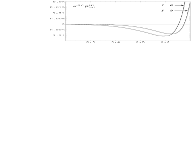
Figure 2: The vacuum effective pressures $a^{D+1}p_{\mathrm{(int)}}^{(j)}$, $j=a,b$, determining the ’interaction’ forces between the plates, as functions on $a/b$ for a massless minimally coupled scalar field in $D=3$ with Robin coefficients $\beta_{a}=0$ and $\beta_{b}=1/5$.

For large values of the mass, $ma\gg 1$, the main contribution into the $\omega$-integral comes from the values $\omega\sim\sqrt{m(b-a)}$. By using the uniform asymptotic expansions for the Bessel modified functions, to the leading order one finds

$$p_{\mathrm{(int)}}^{(j)}\approx\frac{B_{j}^{2}m^{\frac{D}{2}+3}e^{2m(a-b)}\sqrt{ab}}{(4\pi)^{\frac{D}{2}}c_{l}(m)[A_{j}-n^{(j)}B_{j}m]^{2}j(b-a)^{\frac{D}{2}}},$$ (4.8)

for $B_{j}\neq 0$, $j,l=a,b$, $j\neq l$. For $B_{j}=0$ the leading term is the same as that for the $A_{j}=0$ case. The latter is obtained from (4.8).

5 Conclusion

The use of general coordinate transformations in quantum field theory in flat spacetime leads to an infinite number of unitary inequivalent representations of the commutation relations with different vacuum states. In particular, the vacuum state for a uniformly accelerated observer, the Fulling–Rindler vacuum, turns out to be inequivalent to that for an inertial observer, the Minkowski vacuum. In the present paper we have considered the positive frequency Wightman function, the VEVs of the field square and the energy-momentum tensor for a scalar field in the region between two infinite parallel plates moving by uniform proper accelerations, assuming that the field is prepared in the Fulling-Rindler vacuum state and satisfies the Robin boundary conditions on the plates. The general case is investigated when the constants in the Robin boundary conditions are different for separate plates. The boundaries and boundary conditions are static in the Rindler coordinates and no Rindler quanta are created. The only effect of the imposition of boundary conditions on a quantum field is the vacuum polarization. The Wightman function is presented in the form of the mode sum involving series over zeros $\omega=\omega_{n}$ of the function $Z_{i\omega}(\lambda a,\lambda b)$ defined by relation (2.12). For the summation of these series we have applied a summation formula derived in Appendix A by using the generalized Abel-Plana formula. This allowed to extract from the Whightman function the part due to a single plate and to present the additional part in terms of integrals, exponentially convergent in the coincidence limit. The single plate part is investigated previously in Ref [12]. The contribution induced by the second boundary is presented in two alternative forms, Eqs. (2.19), (2.25), obtained from each other by replacements (2.30). In Section 3, by using the expression for the Wightman function, we evaluate the VEVs of the field square and the energy-momentum tensor. The latter is diagonal and the corresponding components are determined by relation (3.17). Various limiting cases are studied. In the limit of small distances between the plates, to the leading order, the VEVs are the same as those for two parallel plates in the Minkowski vacuum. In the near horizon limit, $a,b\rightarrow 0$, the proper accelerations of the plates are large. For fixed values $a/b$ and $\xi/b$, the VEVs grow as $b^{1-D}$ for the field square and as $b^{-1-D}$ for the components of the energy-momentum tensor. In the limit when the world line of the left plate tends to the Rindler horizon, $a\rightarrow 0$, for a fixed proper accelerations of the right plate and the observer, the VEVs induced by the left plate vanish as $\ln^{-2}(2b/a)$ for both the field square and energy-momentum tensor. For large values of the mass, the both single plate and interference parts of the VEVs are exponentially suppressed. The vacuum forces acting on boundaries are determined by ${}_{1}^{1}$-component of the stress and are investigated in Section 4. These forces are presented as the sums of two terms. The first ones correspond to the forces acting on a single boundary then the second boundary is absent. Due to the surface divergences in the VEVs of the energy-momentum tensor, these forces are infinite and need an additional renormalization. The another terms in the vacuum forces are finite and are induced by the presence of the second boundary. They correspond to the ’interaction’ forces between the plates. These forces per unit surface are determined by formula (4.2). For small distances between the plates, to the leading order the standard Casimir result on background of the Minkowski vacuum is rederived. In this limit the ’interaction’ forces are repulsive in the case of Dirichlet boundary condition on one plate and non-Dirichlet boundary condition on the another, and are attractive for all other cases. For large distances, the ’interaction’ forces can be either attractive or repulsive in dependence of the coefficients in the boundary conditions. In Figure 2 we have presented an example when the vacuum ’interaction’ forces are repulsive for small distances and are attractive for large distances. This provides a possibility for the stabilization of the interplate distance by vacuum forces. However, it should be noted that to make reliable predictions regarding quantum stabilization, the renormalized single plate parts $p_{1}^{(j)}$ also should be taken into account. The calculation of these quantities lies on the same line with the evaluation of the total Casimir energy and surface densities and will be presented in the forthcoming paper [32].

In the present paper we have investigated the VEV of the bulk energy-momentum tensor. For scalar fields with general curvature coupling and Robin boundary conditions, in Ref. [33] it has been shown that in the discussion of the relation between the mode sum energy, evaluated as the sum of the zero-point energies for each normal mode of frequency, and the volume integral of the renormalized energy density for the Robin parallel plates geometry it is necessary to include in the energy a surface term concentrated on the boundary (see also the discussion in Ref. [35, 36]). Similar issues for the spherical and cylindrical boundary geometries and in braneworld scenarios are discussed in Refs. [37, 38, 39]. An expression for the surface energy-momentum tensor for a scalar field with a general curvature coupling parameter in the general case of bulk and boundary geometries is derived in Ref. [15]. The investigation of the total Casimir energy, the surface densities, and the energy balance for the geometry under consideration will be reported in [32].

The formulas derived in this paper can be used to generate the vacuum densities for a conformally coupled massless scalar field in de Sitter spacetime in presence of two curved branes on which the field obeys the Robin boundary conditions with coordinate dependent coefficients. The corresponding procedure is similar to that realized in Ref. [17] for the geometry of a single brane and is based on the conformal relation between the Rindler and de Sitter line elements. The results obtained above can be also applied to the geometry of two parallel plates near the $D=3$ ”Rindler wall.” This wall is described by the static plane-symmetric distribution of the matter with the diagonal energy-momentum tensor $T_{i}^{k}=\mathrm{diag}(\varepsilon_{m},-p_{m},-p_{m},-p_{m})$ (see Ref. [40]). Below we will denote by $x$ the coordinate perpendicular to the wall and will assume that the plane $x=0$ is at the center of the wall. If the plane $x=x_{s}$ is the boundary of the wall, when the external ($x>x_{s}$) line element with the time coordinate $t$ can be transformed into form (2.3) with

$$\xi(x)=x-x_{s}+\frac{1}{2\pi\sigma_{s}},\quad\tau=2\pi\sigma_{s}\sqrt{g_{00}(x_{s})}t.$$ (5.1)

In this formula the parameter $\sigma_{s}$ is the mass per unit surface of the wall and is determined by the distribution of the matter:

$$\sigma_{s}=2\int_{0}^{x_{s}}\left(\varepsilon_{m}+3p_{m}\right)\left[\frac{g(x)}{g(x_{s})}\right]^{1/2}dx.$$ (5.2)

For the ”Rindler wall” one has $g_{22}^{\prime}(x)|_{x=0}<0$ [40] (the external solution for the case $g_{22}^{\prime}(x)|_{x=0}>0$ is described by the standard Taub metric). Hence, the Wightman function, the VEVs for the field square and the energy-momentum tensor in the region between two plates located at $x=x_{1}$ and $x=x_{2}$, $x_{i}>x_{s}$ near the ”Rindler wall” are obtained from the results given above substituting $\xi_{i}=\xi(x_{i})$, $i=1,2$ and $\xi=\xi(x)$. For $\sigma_{s}>0$, $x\geq x_{s}$ one has $\xi(x)\geq\xi(x_{s})>0$ and the Rindler metric is regular everywhere in the external region.

6 Acknowledgements

The authors are grateful to Armen Yeranyan for useful discussions. This work was supported by the Armenian National Science and Education Fund (ANSEF) Grant No. 05-PS-hepth-89-70 and by the Armenian Ministry of Education and Science Grant No. 0124.

Appendix A Summation formula over zeros of $Z_{iz}(u,v)$

As we have seen in section 2, the Whightman function for a scalar field in the region between two plates  uniformly accelerated through the Fulling-Rindler vacuum is expressed in terms of series over the zeros $z=\omega_{n}$ of the function $Z_{iz}(u,v)$, $v>u$, defined by formula (2.12). To derive a summation formula for these series, we choose in the generalized Abel-Plana formula [25] the functions

$$\begin{split}f(z)=&\frac{2i}{\pi}\sinh\pi z\,F(z),\\ g(z)=&\frac{\bar{I}_{iz}^{(b)}(v)\bar{I}_{-iz}^{(a)}(u)+\bar{I}_{iz}^{(a)}(u)\bar{I}_{-iz}^{(b)}(v)}{Z_{iz}(u,v)}F(z),\end{split}$$ (A.1)

with a meromorphic function $F(z)$ having poles $z=z_{k}$ ($\neq\omega_{n}$), $\mathrm{Im}\,z_{k}\neq 0$, in the right half-plane $\mathrm{Re}\,z>0$. The zeros $\omega_{n}$ are simple poles of the function $g(z)$. By taking into account the relation

$$g(z)\pm f(z)=\frac{2\bar{I}_{\mp iz}^{(a)}(u)\bar{I}_{\pm iz}^{(b)}(v)}{Z_{iz}(u,v)}F(z),$$ (A.2)

for the function $R[f(z),g(z)]$ in the generalized Abel-Plana formula one obtains

$$R[f(z),g(z)] = 2\pi i\left[\sum_{n=1}^{\infty}\frac{\bar{I}_{-i\omega_{n}}^{(b)}(v)\bar{I}_{i\omega_{n}}^{(a)}(u)}{\frac{\partial}{\partial z}Z_{iz}(u,v)|_{z=\omega_{n}}}F(\omega_{n})\right.$$ (A.3)

$$+ \left.\sum_{k}\underset{{z=z_{k}}}{\mathrm{Res}}\frac{F(z)}{Z_{iz}(u,v)}\bar{I}_{i\sigma(z_{k})z}^{(b)}(v)\bar{I}_{-i\sigma(z_{k})z}^{(a)}(u)\right],$$

where the zeros $\omega_{n}$ are arranged in ascending order, and $\sigma(z_{k})=\mathrm{sgn}(\mathrm{Im\,}z_{k})$. Substituting relations (A.2) and (A.3) into the generalized Abel-Plana formula, as a special case the following summation formula is obtained:

$$\sum_{n=1}^{\infty}\frac{\bar{I}_{-i\omega_{n}}^{(b)}(v)\bar{I}_{i\omega_{n}}^{(a)}(u)}{\frac{\partial}{\partial z}Z_{iz}(u,v)|_{z=\omega_{n}}}F(\omega_{n}) = \frac{1}{\pi^{2}}\int_{0}^{\infty}dz\sinh\pi z\,F(z)$$ (A.4)

$$- \sum_{k}\underset{{z=z_{k}}}{\mathrm{Res}}\frac{F(z)}{Z_{iz}(u,v)}\bar{I}_{i\sigma(z_{k})z}^{(b)}(v)\bar{I}_{-i\sigma(z_{k})z}^{(a)}(u)$$

$$- \int_{0}^{\infty}dz\frac{F(ze^{\frac{\pi i}{2}})+F(ze^{-\frac{\pi i}{2}})}{2\pi Z_{z}(u,v)}\bar{I}_{z}^{(a)}(u)\bar{I}_{-z}^{(b)}(v).$$

Here the condition for the function $F(z)$ is easily obtained from the corresponding condition in the generalized Abel–Plana formula by using the asymptotic formulas for the Bessel modified function and has the form

$$|F(z)|<\epsilon(|z|)e^{-\pi\mathrm{Re\,}z}\left(\frac{v}{u}\right)^{2|\mathrm{Im\,}z|},\quad\mathrm{Re\,}z>0,$$ (A.5)

for $|z|\rightarrow\infty$, where $|z|\epsilon(|z|)\rightarrow 0$ when $|z|\rightarrow\infty$. Formula (A.4) can be generalized for the case when the function $F(z)$ has real poles, under the assumption that the first integral on the right of this formula converges in the sense of the principal value. In this case the first integral on the right of Eq. (A.4) is understood in the sense of the principal value and residue terms from real poles in the form $\sum_{k}\underset{{z=z_{k}}}{\mathrm{Res}}g(z)$, ${\mathrm{Im}\,z}_{k}=0$, have to be added to the right-hand side of this formula, with $g(z)$ from (A.1). For the case of series in Eq. (2.17) the function $F(z)$ is an analytic function and the residue terms in Eq. (A.4) are absent.

References

- [1] V.M. Mostepanenko and N.N. Trunov, The Casimir Effect and Its Applications (Oxford University Press, Oxford, 1997).
- [2] G. Plunien, B. Muller, and W. Greiner, Phys. Rep. 134, 87 (1986).
- [3] K.A. Milton, The Casimir Effect: Physical Manifestation of Zero–Point Energy (World Scientific, Singapore, 2002).
- [4] M. Bordag, U. Mohidden, and V.M. Mostepanenko, Phys. Rep. 353, 1 (2001).
- [5] S.A. Fulling, Phys. Rev D 7, 2850 (1973).
- [6] D.G. Boulware, Phys. Rev. D 11, 1404 (1975).
- [7] W.G. Unruh, Phys. Rev. D 14, 870 (1976).
- [8] S.A. Fulling, J. Phys. A 10, 917 (1977).
- [9] U.H. Gerlach, Phys. Rev. D 40, 1037 (1989).
- [10] N.D. Birrell and P.C.W. Davies, Quantum Fields in Curved Space (Cambridge University Press, Cambridge, England, 1982).
- [11] P. Candelas and D. Deutsch, Proc. R. Soc. Lond. A 354, 79 (1977).
- [12] A.A. Saharian, Class. Quantum Grav. 19, 5039 (2002).
- [13] R.M. Avagyan, A.A. Saharian, and A.H. Yeranyan, Phys. Rev. D 66, 085023 (2002).
- [14] A.A. Saharian, R.S. Davtyan, and A.H. Yeranyan, Phys. Rev. D 69, 085002 (2004).
- [15] A.A. Saharian, Phys. Rev. D 69, 085005 (2004).
- [16] A.A. Saharian, M.R. Setare, Class. Quantum Grav. 21, 5261 (2004).
- [17] A.A. Saharian and M.R. Setare, Phys. Lett. B 584, 306 (2004).
- [18] J. Ambjorn and S. Wolfram, Ann. Phys. (N.Y.) 147, 33 (1983).
- [19] H. Luckock, J. Math. Phys. 32, 1755 (1991).
- [20] G. Esposito, A. Yu. Kamenshchik, and G. Polifrone, Euclidean Quantum Gravity on Manifolds with Boundary (Kluwer, Dordrecht, 1997).
- [21] S.N. Solodukhin, Phys. Rev. D 63, 044002 (2001).
- [22] T. Gherghetta and A. Pomarol, Nucl. Phys. B 586, 141 (2000).
- [23] A. Flachi and D.J. Toms, Nucl. Phys. B 610, 144 (2001).
- [24] A.A. Saharian, Nucl. Phys. B 712, 196 (2005).
- [25] A.A. Saharian, Izv. Akad. Nauk Arm. SSR. Mat. 22, 166 (1987) [Sov. J. Contemp. Math. Anal. 22, 70 (1987)]; A.A. Saharian, ”The generalized Abel–Plana formula. Applications to Bessel functions and Casimir effect”, Report No. IC/2000/14; hep-th/0002239.
- [26] U.H. Gerlach, Phys. Rev. D 59, 104009 (1999).
- [27] U.H. Gerlach, Found. Phys. 33, 179 (2003).
- [28] M. Abramowitz and I.A. Stegun, Handbook of Mathematical functions (National Bureau of Standards, Washington, DC, 1964).
- [29] C.T. Hill, Nucl. Phys. B 277, 547 (1986).
- [30] S. Tagaki, Prog. Theor. Phys. 74, 142 (1985).
- [31] H. Ooguri, Phys. Rev. D 33, 3573 (1986).
- [32] A.A. Saharian and R.S. Davtyan, in preparation.
- [33] A. Romeo and A.A. Saharian, J. Phys. A 35, 1297 (2002).
- [34] H. Matevosyan and A.A. Saharian, unpublished.
- [35] S.A. Fulling, J. Phys. A 36, 6857 (2003).
- [36] K.A. Milton, J. Phys. A 37, R209 (2004).
- [37] A.A. Saharian, Phys. Rev. D 63, 125007 (2001).
- [38] A. Romeo and A.A. Saharian, Phys. Rev. D 63, 105019 (2001).
- [39] A.A. Saharian, Phys. Rev. D 70, 064026 (2004).
- [40] R.M. Avakyan, E.V. Chubaryan, and A.H. Yeranyan, ”’Homogeneous’ Gravitational field in General Relativity?,” gr-qc/0102030.