On the chaos of D-brane phase transitions

Abstract:

We study small instanton (and brane recombination) phase transitions in phenomenological models built with D-branes. By explicitly describing the cosmological dynamics of the moduli and matter fields, we show that these transitions do not occur smoothly, but are typically chaotic with the gauge group of the low energy theory fluctuating in time. We comment on the potential implications for cosmological questions such as inflation.

1 Introduction: phase transitions on D-branes

There are good reasons to believe that there was a “pre-thermal epoch” of the Universe in which phase transitions occurred that were driven by the movement of moduli fields along flat or almost flat directions. In this epoch gauge symmetries may have been restored instead of broken, and there is no a priori reason why symmetries could not have been broken and restored more than once. If this happened in the early Universe it would have far reaching implications for such issues as inflation, baryogenesis and dark matter. It is of great interest therefore to examine cases where moduli driven phase transitions can be analysed in more detail than usual, especially if these cases display such anomalous behaviour.

The transitions we will discuss in this paper are of the so-called small instanton type [1]. They are known to occur in both M-theory [2] and D-brane models [3], but remarkably in the latter they can be analysed completely in the small coupling and large volume limits in terms of the effective field theory. This is largely due to the fact that the extra light degrees of freedom which appear during such transitions are “particles” rather than tensionless non-critical strings as would be the case in the M-theory equivalent. There are two complementary pictures of what happens during a small instanton phase transition in type II models: the more straightforward involves a low (e.g. 3) dimensional D-brane impacting and dissolving on a stack of higher (e.g. 7) dimensional ones; the less straightforward picture is the T-dual process, in which for example two intersecting D6-branes undergo recombination. The brane recombination picture provides a nice geometric realisation of symmetry breaking, but either way the transition, when it evolves in this direction, is to a theory with a gauge symmetry of lower rank. The issues we raise are therefore relevant to phase transitions in the wide class of Standard Model (SM)-like models built from intersecting or coincident D-branes [4, 5, 6, 7, 8]. Indeed it may even be possible to find the SM itself, with electroweak symmetry breaking realised in just such a manner [8].

In this work we examine the properties of these transitions when they take place in a cosmological setting. At first sight it seems reasonable to suppose (and it has usually been assumed) that such transitions would occur smoothly, with the lower dimensional D-brane dissolving “monotonically” in the higher dimensional one. However we uncover some quite unexpected properties. The reason behind this is that the effective action describing the transition is related to one of the simplest chaotic systems. This leads to rather curious physical phenomena, in which for example the low dimension brane dissolves temporarily in the high dimension one, only to be ejected at some later time. In addition there is an attractor mechanism which means that the lower dimensional D-brane never leaves the vicinity of the higher dimensional one for very long. However it cannot ever be said to have fully dissolved in it either; the dissolved brane never completely spreads out, and in fact this would require some additional ingredient such as supersymmetry breaking. (The picture we describe here is valid at scales significantly above the supersymmetry breaking scales suggested by phenomenology and also at small coupling and low velocities.) One additional feature which is of some interest is that the potential has a term that is quartic in the instanton radius. The instanton size is therefore constricted by the compact volume, an additional factor working against the completion of the phase transition.

The set-up

The setting for our discussion is supersymmetric orientifold compactifications of type II models involving various D-brane configurations [9]. We concentrate on ${\cal{N}}=1$ supersymmetric compactifications with non-abelian gauge fields and chiral fermions, which can be built with a gauge group and particle spectrum that is fairly close to the MSSM [4, 7].

Type IIB string theories include D7 and D3-branes. In the vacua we shall be discussing D3-branes are present and are taken to span the four dimensions of normal spacetime to preserve the four dimensional Poincaré invariance of the vacuum. Various stacks of D7-branes are also present and are taken to wrap our four dimensions for the same reason and then each stack must wrap a compact 4 cycle in the orientifold. The number of each type of brane wrapping the various possible cycles is restricted by a set of tadpole cancellation conditions which essentially implement the requirement that the net charge with respect to any form field on a compact manifold is zero. Non-abelian gauge fields and chiral fermions arise in these models on various brane world volumes and intersection loci.

These type IIB constructions are related to other set-ups under various dualities and it is worth briefly reviewing them as for certain situations the alternatives can be more intuitive. First they are mirror to type IIA orientifold constructions including configurations of intersecting D6-branes in the vacuum. Once again the D6-branes are extended in the four directions of our space and time. Their remaining dimensions then wrap compact 3 cycles within the orientifold. In this case non-abelian gauge fields arise on the D6-brane stack world volumes and chiral fermions appear as extra light degrees of freedom where the various D6-brane stacks have four dimensional intersections. Since this type IIA set-up contains purely D6-branes, the only fields that are excited in the background are the dilaton, the Ramond-Ramond one form and of course the metric. In the S-dual picture in terms of eleven dimensional M-theory these quantities all map to various parts of the metric. Therefore the S-dual of these IIA constructions are purely metric ${\cal{N}}=1$ supersymmetric compactifications of eleven dimensional M-theory to four dimensions. In other words these are compactifications of M-theory on manifolds of $G_{2}$ holonomy. The presence of chiral fermions and non-abelian gauge fields in the four dimensional effective theory tells us that these $G_{2}$ compactifications must have various singular surfaces within them. In particular, within the compact space, codimension four singularities exist on which live the non-abelian gauge fields [10, 11]. These intersect at codimension 7 points and it is on these singularities that the chiral fermions arise as extra light states [12, 13, 14].

Let us now return to the type IIB picture. Within this setup the small instanton phase transitions occurs as follows: a D3-brane approaches a D7 brane stack, impinges upon it and dissolves to become an object comprised primarily of D7 gauge fields [15]; the “fundamental” D3-brane disappears and is replaced by a solitonic object, which is essentially a Yang Mills instanton dressed up with the various other fields that exist upon the D7-brane stack; at the moment of dissolution the instanton appears as a point like object in the four dimensions orthogonal to the original D3-brane in the stack’s world volume, but it is then free to spread out to become a solitonic three brane of finite width. From the four dimensional perspective this process looks like a Higgs effect. The easiest way to see this is to consider the four dimensional gauge symmetry which is associated with the D7-brane stack. For a stack of $N$ branes away from any special points within the orientifold for example, and in the absence of any expectation values for the fields living on the D7-branes, this is simply $U(N)$. As the D3-brane dissolves onto the the D7-brane stack during the small instanton transition it gives rise to a non-vanishing vacuum expectation value for the gauge fields associated with an $SU(2)$ subgroup of this $U(N)$. This is simply because the the Yang Mills instanton on which the emerging solitonic object is based is valued within $SU(2)$. As the relevant gauge field components have their indices lying within the compact space this corresponds, in the four dimensional effective theory, to giving $SU(2)$ valued expectation values to Higgs fields.

This phenomenon will have duals in the IIA and M-theoretic pictures. In IIA intersecting D6-brane models this process corresponds to the collision of various D-brane stacks at four dimensional intersections and their resulting recombination via some “fuzzy” process [7, 16]. Naturally the equivalent of this process in $G_{2}$ compactifications is the recombination of codimension 4 singularities after collision at a codimension 7 point. We should add that in the IIB picture we will neglect fluxes on the D7 world volumes. In the IIA picture this corresponds to the intersection angles being very small or zero. Extension to the more realistic cases of finite intersection angles will be considered in a future work.

We now proceed to examine the dynamics of these processes. We present the discussion in the type IIB language as this is the easiest in which to phrase our methodology. However our results may be made applicable to the other cases simply by taking the relevant mirror and then S dualities.

The rest of this paper is structured as follows. In section 2 we briefly review the relevant aspects of the realisation of the ADHM description of instantons in D-brane physics. In section 3 we describe how this becomes embedded in string phenomenological models. Section 4 solves the resulting system to describe the dynamics of small instanton transitions and discusses the late time behaviour of our system, and its implications for cosmology.

2 Instantons in D-brane physics

We begin by recalling how the ADHM instanton construction of self dual Yang Mills configurations [17], specifically single Yang Mills instantons, is realised in D-brane physics [15]. This will be crucial in understanding the physical interpretation of the description of the small instanton transition process later on. We shall start with the realisation of the ADHM formalism for uncompactified D-brane world volumes, highlighting the ${\cal{N}}=2$ structure, and then describe how this is modified when some of the branes are wrapped upon compact cycles. Phenomenological models are ${\cal{N}}=1$ supersymmetric and so have to be presented in suitable terms, thus in the next section we will have to translate this into the ${\cal{N}}=1$ language, add in moduli dependence and so forth.

The realisation of the ADHM formalism in a D-brane context has been understood for a number of years [15]. The system we shall concentrate on comprises a D3-brane lying within a stack of $N$ D7-branes in type IIB. As described above, we shall take six of the ten dimensions of space and time to be compactified on some appropriate compact space. The D3-branes are taken to be oriented transversely to this compact space and the D7-brane stack will be taken to wrap a four dimensional submanifold within it.

Now let us examine the effective four dimensional theory associated with this set-up. First consider the limit in which the volume of the 4 cycle which the D7-branes wrap is infinite; the world volume of the D7-brane is then also infinite, and consequently the gauge coupling of the D7-brane gauge symmetry (which is inversely proportional to the volume of the D7s) is zero. In this limit therefore there is no contribution to the potential of the $d=4$ system, which we take to be ${\cal{N}}=2$ supersymmetric for now, from the $D$-term associated with the D7 stack. We shall denote the ${\cal{N}}=2$ hypermultiplets arising from strings stretching between the D3-brane and D7-brane stack as $\chi_{ai}$, where $i$ is the ${\cal{N}}=2$ $SU(2)$ automorphism index and $a$ is the $U(N)$ gauge index. (We will frequently refer to these states as ‘twisted’ because they are associated with non-integer mode expansions.) In addition we shall write the scalar fields corresponding to the collective coordinates of the D3-brane and the D7 stack in the two codimensions of the D7-branes as $X^{I}$ and $X^{{}^{\prime}J}$ respectively. The scalar potential for the system in this “infinite D7 volume limit” is then given by

$$V_{\textnormal{{Vol}}(T^{4})\rightarrow\infty}=\frac{g_{D3}^{2}}{4}\sum_{A=1}^{3}(\chi_{ia}^{\dagger}\sigma_{ij}^{A}\chi_{aj})^{2}+\sum_{I=1}^{2}\frac{(X^{I}-X^{{}^{\prime}I})^{2}}{2\pi\alpha^{\prime}}\chi^{\dagger}\chi$$ (1)

where $\sigma^{A}$ are the Pauli matrices. We note for later that the gauge coupling $g_{D_{3}}$ is a function of the dilaton and moduli fields. At the moment we assume that these are frozen, but in the next section we shall have to include these as full dynamical degrees of freedom.

The potential has two branches of zeros. The first of these, the Coulomb branch, corresponds to setting $\chi=0$ and then allowing the separation of the branes to be arbitrary. This just corresponds to the D3-brane and the D7 stack being free to move about in the transverse space while not interacting with each another. The second branch of zeros, the Higgs branch, is given by setting the separation of the D-branes to zero so that the the D3-brane lies on top of the D7 stack and then demanding that the D-flatness condition associated with the D3-brane world volume gauge theory is satisfied,

$$\chi_{ia}^{\dagger}\sigma_{ij}^{A}\chi_{aj}=0.$$ (2)

It turns out that there is a precise connection between these D-flatness conditions and the equations describing the collective coordinates of localised instanton solutions on the D7-brane stack. Indeed the above equation is none other than the ADHM constraint equations in the canonical form for a solution with a single unit of instanton charge in a $U(N)$ gauge theory, where $\chi$ is interpreted as the ADHM data. The fields $\chi$ also have the $U(1)$ symmetry required to complete the ADHM hyperKähler quotient: this is simply the $U(1)$ of the gauge theory on the D3 world volume. The general set of solutions to the D3 flatness condition of the Higgs branch is then given by the following:

$$\chi_{ai}=\rho U_{ab}m_{bi}.$$ (3)

Here $\rho$ can be interpreted as the size of the instanton, $U$ is an $\frac{SU(N)}{SU(N-2)\times U(1)}$ matrix containing the gauge orientation and embedding moduli of the instanton within the gauge group and $m_{bi}=\delta_{bi}$. The bottom line is that one can interpret the expectation values of the twisted sector fields as describing the collective coordinates of a Yang-Mills instanton configuration living in the D7 world volume, and that this branch of solutions corresponds to a situation where the D3-brane has dissolved upon the D7 stack. The degrees of freedom associated with the Higgs branch are then just the collective coordinates of the soliton that the D3-brane has become, which are in one to one correspondence with the degrees of freedom of the Yang Mills instanton on which the soliton is based (The associated instanton solution itself can be detected by probe calculations if needs be [15]).

This then is the situation when the world volume of the D7 stack is taken to be infinite. How are things modified when we allow the D7 branes to wrap a submanifold of finite size? In this case there is an additional contribution to the potential of the four dimensional theory. This contribution comes from the D-terms associated with the D7 world volume gauge theory, the gauge coupling of which is now finite. The potential is now

$$V=\frac{g_{D7}^{2}}{4}\sum_{A=1}^{3}\sum_{a=1}^{N^{2}}(\chi_{ic}^{\dagger}\sigma_{ij}^{A}t_{cd}^{(a)}\chi_{jd})^{2}+\frac{g_{D3}^{2}}{4}\sum_{A=1}^{3}(\chi_{ia}^{\dagger}\sigma_{ij}^{A}\chi_{ja})^{2}+\sum_{I=1}^{2}\frac{(X^{I}-X^{{}^{\prime}I})^{2}}{2\pi\alpha^{\prime}}\chi^{\dagger}\chi+\ldots$$ (4)

where the ellipsis indicates terms in the potential such as $D$-terms involving the $X^{I}$ fields that are zero in the interesting directions in field space. Here the $t$’s are the generators of the $U(N)$ gauge group. Again the couplings $g_{D_{3}}$ and $g_{D_{7}}$ will be different functions of the moduli fields describing the compact space.

Evidently the Coulomb branch of solutions is unaffected by the finiteness of the compact space: the D3 and D7-branes can still move about unhindered in the transverse space if the twisted sector is not excited. The Higgs branch though is affected by the presence of the new term. In this branch the potential reduces to the first two terms above. As they are both positive definite for a zero of the potential they must vanish independently at the global minimum. The vanishing of the second term simply implies the D3 $D$-flatness condition as before. Thus any putative flat direction that remains when the D7 volume is finite would then be a subspace of the instanton moduli space. The question is if there is indeed a subspace of the instanton moduli space that remains flat even in the presence of the extra potential terms. The answer is no: substituting a general solution to the D3 $D$-flatness conditions into the first term in the potential we obtain a non-zero contribution which is proportional to the instanton size, $\rho$, to the fourth power. (We shall see this explicitly in the next section.) Consequently the expectation value that would be interpreted as the instanton size is no longer a flat direction in the theory’s moduli space; the dissolution of the D3-brane onto the the D7 stack is no longer associated with a flat direction and there is a term in the potential pushing the instanton size to zero. This result, which will be important later, is in agreement with the fact that there is no single instanton solution to Yang-Mills theory on $T^{4}$ [18, 19]. There is a simple argument that no such solution exists: if a $U(N)$ $k=1$ self-dual solution existed on $T^{4}$ then the Nahm transformation would imply the existence of a $k=N$ $U(1)$ solution on the dual torus! Since it is obvious that no such solution can exist neither can the single charge $U(N)$ configuration.

3 The small instanton transition in type II brane world models

So far we have described the dissolution of D3-branes onto D7-branes in a manner which, apart from the additional contribution due to the finiteness of the compact space, is conventional and in particular is couched in ${\cal{N}}=2$ language. In order to make contact with phenomenological “brane world” models, we have to deal with two things. First we need to go to the more usual ${\cal{N}}=1$ language of phenomenological models, whilst showing that the instanton data sector of the theory retains the essential underlying ${\cal{N}}=2$ structure. Our second problem arises from the fact that the system is not stabilised and therefore we have to allow the moduli fields to become full dynamical degrees of freedom. In particular the couplings $g_{D_{3}}$ and $g_{D_{7}}$ are as we have stressed functions of the moduli and they will change during the cosmological evolution. This means we have to include in the action all of the moduli dependence arising from the Kähler potential of the ${\cal{N}}=1$ theory.

To do this we continue using the type IIB D3/D7-brane picture, and first recall some basic facts about the effective theories of the ${\cal{N}}=1$ models. (The descriptions of the associated processes in type IIA and in G2 compactifications of M-theory, as described in the introduction, can then be obtained by considering the mirror of our discussion and its S-dual.) There are numerous string phenomenological models in the literature which are specifically based upon D3 and D7-brane configurations on orientifolds of Calabi-Yau spaces in type IIB [5, 6]. We shall not concern ourselves with any one particular such vacuum as we wish to keep our considerations as general as possible. Instead we shall just require that the eventual four dimensional theory has ${\cal{N}}=1$ supersymmetry, and will achieve this by compactifying on a space which is an orientifold of an appropriate orbifold, with a covering space that is a product of 2-tori. We will assume that there is a stack of 2 D7-branes wrapping an appropriate 4 cycle which for simplicity does not lie on or pass through any fixed planes of the orientifold. We choose to label the three $T^{2}$ of the orbifold such that these D7-branes wrap tori 1 and 2 and are transverse to torus 3. We shall also require that there is a single D3-brane close to this stack of D7-branes lying in the four dimensions of our space and time. Given this minimal set-up the following ${\cal{N}}=1$ structure describes the relevant moduli in the four dimensional effective description of the system [20, 21, 22, 23, 24, 25]:

$$K = -\ln(S+\bar{S)}-\sum_{i=1}^{3}\ln(T_{i}+\bar{T_{i})}+\sum_{i=1}^{3}\frac{|C_{3}^{i}|^{2}}{T_{i}+\bar{T_{i}}}$$ (5)

$$+\sum_{i=1,j\neq i}^{2}\frac{|C_{i}^{7}|^{2}}{T_{j}+\bar{T}_{j}}+\frac{|C_{3}^{7}|^{2}}{S+\bar{S}}+\frac{1}{2}\frac{(|A|^{2}+|B|^{2})}{\sqrt{(T_{1}+\bar{T}_{1})(T_{2}+\bar{T}_{2})}}$$

$$W=g_{3}(C_{1}^{3}C_{2}^{3}C_{3}^{3}+C_{3}^{3}AB)+g_{7}(C_{1}^{7}C_{2}^{7}C_{3}^{7}+AC^{7}B)$$ (6)

$$h_{D3} = S$$ (7)

$$h_{D7\,\alpha\beta} = T_{3}\,\delta_{\alpha\beta}$$ (8)

Here $g_{3}^{2}=2\pi$ and $g_{7}^{2}=\alpha^{{}^{\prime}2}(2\pi)^{5}$ (not to be confused with the effective couplings in the $D$-terms $g_{D_{3}}$ and $g_{D_{7}}$ which we shall determine shortly) and the $h$’s are the gauge kinetic functions. In these expressions $S$ is the dilaton superfield and $T_{i}$ are the superfields associated with the sizes of the three 2-tori of the orbifold. The $C^{i}_{3}$ superfields are associated with the position of the D3-brane within the compact space and the $C^{7}_{i}$ moduli describe the D7-brane position moduli and the moduli associated with various Wilson lines on the stack’s world volume. Finally the superfields $A$ and $B$ are associated with twisted states of strings stretching between the D3 and D7-branes. These states are massless when the D3/D7-branes are coincident and indeed the mass is proportional to the stretching distance between D3 and D7-branes.

Next we wish (with minimal loss of generality) to truncate the field content to reduce the number of fields we have to consider. However, we still must keep those necessary to describe the phenomena we want to investigate. This truncation must of course be consistent in that a solution to the truncated system should also be a solution to the full one. A consideration of the above shows that the following truncations work:

$$C_{3}^{1}=C_{3}^{2}=0,\,\,\,\,\,C_{1}^{7}=C_{2}^{7}=0,\,\,\,\,\,T_{1}=T_{2}\equiv T\,.$$ (9)

The first of these corresponds to not exciting the D3-brane’s motion parallel to the stack of D7-branes. The second set of constraints corresponds to dropping certain Wilson line moduli associated with the D7 stack. For brane stacks of different dimensionalities it may be of interest to keep such moduli in future solutions, as keeping more than one of these matrix valued brane coordinates could give information about the onset of fuzziness due to cosmological evolution. The final truncation just corresponds to using an obvious symmetry between the $T$ superfields associated with the two $T^{4}$ wrapped by the D7 to simplify our equations. Performing these truncations our system becomes

$$K_{1}=-\ln(S+\bar{S)}-2\ln(T+\bar{T})-\ln(T_{3}+\bar{T_{3})}+\frac{|C_{3}|^{2}}{T_{3}+\bar{T}_{3}}+\frac{|C^{7}|^{2}}{S+\bar{S}}+\frac{1}{2}\frac{(|A|^{2}+|B|^{2})}{T+\bar{T}}$$ (10)

$$W_{1}=g_{3}(C_{3}AB)+g_{7}(AC^{7}B)$$ (11)

where we have dropped the indices on the remaining $C_{3}$ and $C^{7}$ fields as this now causes no ambiguity. It should be noted that we are also suppressing indices describing how $A$,$B$,$C_{3}$ and $C^{7}$ transform under the D-brane gauge groups. The twisted sector states transform under bi-fundamental representations of the two unitary groups and $C_{3}$ and $C^{7}$ are of course in the adjoint of the D3 and D7 gauge groups respectively. Thus the only ambiguity that arises in our suppression of these indices above is in the $AC^{7}B$ term. Here the indices in the fundamental of $U(2)_{D7}$ contract as $A_{\alpha}C_{\,\,\,\,\,\,\,\,\beta}^{7\,\alpha}B^{\beta}$ and from now on it will be useful to use the expansion $C_{\,\,\,\,\,\,\,\beta}^{7\,\alpha}=C^{7\,(a)}t_{\,\,\,\,\beta}^{(a)\,\,\,\alpha}$ where the $t$ are the generators of $U(2)$. More generally in the $U(N)$ case the $t_{(a)}$ are the D7 stack gauge group generators.

We can now turn to the component action form of the scalar sector of the full ${\cal{N}}=1$ supergravity theory; we find

$$S = \int\sqrt{-g}\left[\left(\frac{1}{(S+\bar{S})^{2}}+\frac{2|C^{7\,(a)}|^{2}}{(S+\bar{S})^{3}}\right)\partial S\partial\bar{S}-\frac{1}{(S+\bar{S})^{2}}\left(\partial SC^{7\,(a)}\partial\bar{C}^{7\,(a)}+\partial\bar{S}\bar{C}^{7\,(a)}\partial C^{7\,(a)}\right)\right.$$ (12)

$$+\left(\frac{1}{(T_{3}+\bar{T}_{3})^{2}}+\frac{2|C_{3}|^{2}}{(T_{3}+\bar{T}_{3})^{3}}\right)\partial T_{3}\partial\bar{T}_{3}-\frac{1}{(T_{3}+\bar{T}_{3})^{2}}\left(\partial T_{3}C_{3}\partial\bar{C}_{3}+\partial\bar{T}_{3}\bar{C}_{3}\partial C_{3}\right)$$

$$+\left(\frac{2}{(T+\bar{T})^{2}}+\frac{(|A|^{2}+|B|^{2})}{(T+\bar{T})^{3}}\right)\partial T\partial\bar{T}-\frac{1}{2}\frac{1}{(T+\bar{T})^{2}}\left(\partial T(A\partial\bar{A}+\partial\bar{B}B)+\partial\bar{T}(\partial A\bar{A}+\bar{B}\partial B)\right)$$

$$\left.+\frac{1}{T_{3}+\bar{T}_{3}}\partial C_{3}\partial\bar{C}_{3}+\frac{1}{S+\bar{S}}(\partial C^{7\,(a)}\partial\bar{C}^{7\,(a)})+\frac{1}{2}\frac{1}{T+\bar{T}}(\partial A\partial\bar{A}+\partial\bar{B}\partial B)+V_{F}+V_{D}\right]$$

In the above $V_{F}$ and $V_{D}$ are the contributions to the potential from ${\cal{N}}=1$ $F$-terms and $D$-terms respectively. In our discussion we will only be working to fourth order in the matter fields (as well as applying the slowly moving modulus approximation). In this approximation we find the following expression for $V_{F}$ from the standard ${\cal{N}}=1$ structure:

$$V_{F} = e^{K}\,K^{-1\,\bar{i}j}\bar{F}_{\bar{i}}F_{j}$$ (13)

$$= \frac{1}{(S+\bar{S})(T+\bar{T})^{2}(T_{3}+\bar{T}_{3})}\left[g_{3}^{2}|AB|^{2}(T_{3}+\bar{T}_{3})+g_{7}^{2}\sum_{(a)}|At^{(a)}B|^{2}(S+\bar{S})\right.$$

$$+\left\{\left(g_{3}\bar{C}_{3}\bar{B}+g_{7}\bar{C}^{7\,(a)}\bar{B}t^{(a)}\right)\left(g_{3}C_{3}B+g_{7}C^{7\,(b)}t^{(b)}B\right)\right.$$

$$+\left.\left.\left(g_{3}C_{3}A+g_{7}C^{7\,(a)}At^{(a)}\right)\left(g_{3}\bar{C}_{3}\bar{A}+g_{7}\bar{C}^{7\,(b)}t^{(b)}\bar{A}\right)\right\}2(T+\bar{T})\right]\,.$$

For $V_{D}$ we have

$$V_{D}=\frac{1}{2}Re(h_{D3})^{-1}D^{(D3)}D^{(D3)}+\frac{1}{2}Re(h_{D7^{(a)}})^{-1}D^{(D7^{(a)})}D^{(D7^{(a)})}$$ (14)

where, using the usual formulae for the $D$-terms, we have

$$D^{(D3)}=\frac{g_{3}}{2}\frac{(|B|^{2}-|A|^{2})}{(T+\bar{T})}$$

$$D^{(D7^{(a)})}=\frac{g_{7}}{2}\frac{(At^{(a)}\bar{A}-\bar{B}t^{(a)}B)}{T+\bar{T}}+\frac{g_{7}f_{abc}\bar{C}^{7\,(b)}C^{7\,(c)}}{S+\bar{S}}$$ (15)

where $f_{abc}$ are the $U(N)$ structure constants.

Connection with the ${\cal{N}}=2$ structure

Before proceeding to make further truncations it will now be helpful for us to show explicitly how the ${\cal{N}}=2$ structure and potential described in the previous section is embedded in this result. In order to do this we must first identify the ${\cal{N}}=2$ hypermultiplets associated with the instanton data. These fields must be composed out of a non-holomorphic combination of fields from the ${\cal{N}}=1$ viewpoint as the $SU(2)$ automorphism index which they carry is associated with the different possible choices of complex structure associated with the ${\cal{N}}=2$ theory; clearly if we are writing things in terms of the ${\cal{N}}=1$ language then we have chosen one particular such complex structure. In fact, given that $A$ and $\bar{B}$ have the same charge under the $U(2)$ associated with the D7 stack, we are led to suggest the identification $\chi_{1\,\alpha}=A_{\alpha}$ and $\chi_{2\,\alpha}=\bar{B}_{\alpha}.$

To show this identification is correct we will now recover the potential given in the previous section from that given above in the theory derived from the ${\cal{N}}=1$ structure. The D-terms in the ${\cal{N}}=2$ potential come in the ${\cal{N}}=1$ language from both $D$ and $F$ terms where, to obtain parity with the previous section, we set the metric moduli and dilaton to be constant. The contribution to the potential given above coming from the sum of the $D^{2}$ term of the D3-brane and the $|F_{C_{3}}|^{2}$ term is

$$V_{D3}=\frac{g_{3}^{2}(4|AB|^{2}+(|A|^{2}-|B|^{2})^{2})}{4(S+\bar{S})(T+\bar{T})^{2}}.$$ (16)

To show that this is compatible with our identification of the ${\cal{N}}=2$ structure, we use,

$$\sum_{A}^{3}(\chi_{i\gamma}^{\dagger}\sigma_{ij}^{A}\chi_{j\gamma})^{2} = 4|\bar{\chi}_{1}\chi_{2}|^{2}+(\bar{\chi}_{1}\chi_{1}-\bar{\chi}_{2}\chi_{2})^{2}$$ (17)

$$= 4|AB|+(|A|^{2}-|B|^{2})^{2}$$

where we have suppressed contracted gauge group indices as elsewhere in this section. This contribution to the potential can then be written as

$$V_{D3}=\frac{g_{3}^{2}}{4(S+\bar{S})(T+\bar{T})^{2}}\,\sum_{A}^{3}(\chi_{i\gamma}^{\dagger}\sigma_{ij}^{A}\chi_{j\gamma})^{2}.$$ (18)

If we identify $g_{D_{3}}=g_{3}/\sqrt{(S+\bar{S})(T+\bar{T})^{2}}$, we then see that this term reproduces the contribution to the potential coming from the ${\cal{N}}=2$ $D$-term associated with the D3-brane, as seen in the previous section. Note that the correct identification relies on specific couplings in the ${\cal{N}}=1$ superpotential and also on the correct relation between the Kähler potential and gauge kinetic function.

Similarly the contribution to our potential from the $D^{2}$ terms from the D7-branes, plus the $|F_{C_{7}}|^{2}$ term is

$$V_{D7}=\frac{g_{7}^{2}(\sum_{a=1}^{4}4|At^{(a)}B|^{2}+\sum_{a=1}^{4}(At^{(a)}\bar{A}-\bar{B}t^{(a)}B)^{2})}{4(T+T)^{2}(T_{3}+\bar{T}_{3})}.$$ (19)

Comparing this with

$$\sum_{A}^{3}(\chi_{i\alpha}^{\dagger}t_{\,\,\,\,\,\beta}^{(a)\,\alpha}\sigma_{ij}^{A}\chi_{j}^{\beta})^{2} = 4|\bar{\chi}_{1}t^{(a)}\chi_{2}|^{2}+(\bar{\chi}_{1}t^{(a)}\chi_{1}-\bar{\chi}_{2}t^{(a)}\chi_{2})^{2}$$ (20)

$$= 4|At^{(a)}B|^{2}+(At^{(a)}\bar{A}-\bar{B}t^{(a)}B)^{2}$$

we find the expression

$$V_{D7}=\frac{g_{7}^{2}}{4(T+\bar{T})^{2}(T_{3}+\bar{T}_{3})}\,\sum_{a=1}^{4}\sum_{A}^{3}(\chi_{i\alpha}^{\dagger}t_{\,\,\,\,\,\beta}^{(a)\,\alpha}\sigma_{ij}^{A}\chi_{j}^{\beta})^{2}.$$ (21)

Thus defining $g_{D7}=g_{7}/\sqrt{(T+\bar{T})^{2}(T_{3}+\bar{T}_{3})}$ we find that these terms reproduce the contribution to the potential of the previous section from the ${\cal{N}}=2$ D7 D-terms.

The action for cosmology

Having confirmed the embedding of the ${\cal{N}}=2$ structure of the previous section within the ${\cal{N}}=1$ language, it is now straightforward to identify the ${\cal{N}}=1$ fields that correspond to the collective coordinates of an instanton: we simply use equation (3) and the relationship we have established between the two descriptions. We find that if the twisted sector fields take the form,

$$A_{\alpha} = \rho(-i\theta_{3}+\theta_{4},\,-i\theta_{1}-\theta_{2})$$ (22)

$$B^{\alpha} = \rho(i\theta_{1}+\theta_{2},\,-i\theta_{3}+\theta_{4})$$ (23)

where $\sum_{n=1}^{4}\theta_{n}^{2}=1$ then they describe the collective coordinates of an instanton of size $\rho$ and with $SU(2)$ orientation moduli given by the $\theta$’s.

The next step is to identify a consistent truncation of our theory that includes $A$ and $B$ in the form given in equations (22) and (23), so that we can interpret some of our fields as describing an instanton on the D7 stack in the compactified dimensions which it wraps. Inspection of the component form of the scalar sector of the theory shows that the following truncations are consistent when taken together. Firstly we set $C^{7(a)}=0$ unless $a$ labels the identity matrix generator. In other words we just keep the D7 modulus corresponding to the overall position of our stack of D-branes and discard moduli which describe such phenomena as the stack separating. We will also truncate numerous axions such as the imaginary parts of the $S$, $T$ and $T_{3}$ superfields. We write $C^{7\,(1)}=R(\cos(\psi)+i\sin(\psi))$ and $C_{3}=r(\cos(\chi)+i\sin(\chi))$ and then truncate $\psi$ and $\chi$. This last truncation corresponds to having both branes simply moving along the radial direction from some arbitrarily chosen origin in the two dimensional subspace of the orientifold transverse to the D7-brane stack. Finally we make what we shall refer to as the ADHM truncation which simply corresponds to setting $A$ and $B$ to the values given above.

After these simplifications we are left with the following consistent truncation of the original theory:

$$S = \int\sqrt{-g}\left[\mathcal{R}+\frac{1}{4}(\partial\phi)^{2}+\frac{1}{4}(\partial\beta_{3})^{2}+\frac{1}{2}(\partial\beta)^{2}+\frac{1}{2}e^{-\phi}(\partial R)^{2}+\frac{1}{2}e^{-\beta_{3}}(\partial r)^{2}\right.$$ (24)

$$\left.+\frac{1}{2}e^{-\beta}(\partial\rho)^{2}+\frac{3}{32}g_{7}^{2}\rho^{4}e^{-2\beta-\beta_{3}}+(g_{3}r+\frac{g_{7}}{2}R)^{2}\frac{1}{2}\rho^{2}e^{-\phi-\beta-\beta_{3}}\right]$$

In the above we have reinstated the four dimensional Einstein-Hilbert term and we have also used the following definitions:

$$Re\{S\} = e^{\phi}+\frac{1}{2}R^{2}$$

$$Re\{T\} = e^{\beta}+\frac{1}{2}\rho^{2}$$

$$Re\{T_{3}\} = e^{\beta_{3}}+\frac{1}{2}r^{2}.$$ (25)

To summarise the fields appearing in the action: $\phi$ is interpreted as the four dimensional dilaton; the fields $\beta$ and $\beta_{3}$ describe the size moduli associated with the spaces wrapped by and transverse to the D7-brane stack respectively; the fields $R$ and $r$ describe radial motion of the D7 stack and D3-brane respectively relative to some origin in the third torus of the orbifold; finally $\rho$ describes the size of the instanton which results when the D3-brane dissolves upon the stack of D7-branes. Note that the potential found in this action has the properties we would expect from the above discussion. In particular when $(g_{3}r+\frac{g_{7}}{2}R)=0$ so that we are in the Higgs branch the potential is proportional to $g_{7}^{2}$ indicating that it comes from $F$ and $D$-terms associated with the D7-brane and is proportional to the size of the instanton to the fourth power, $\rho^{4}$. Thus as described in the previous section we find that the flat direction corresponding to the size of an instanton in the D3/D7-brane system in an infinite volume is no longer flat after compactification.

One question that could be asked about this “ADHM-like” truncation we have chosen is whether it is actually preferred in some sense. To answer this we can examine the structure of the potential before this truncation, by replacing $|A|^{2}=x$ , $|B|^{2}=y$ and $|A.B|=z$ and treating $x,y,z$ as independent. Using the standard $U(2)$ identity $\frac{1}{2}\delta_{\beta}^{\alpha}\delta_{\delta}^{\gamma}=t_{\,\delta}^{(a)\alpha}t_{\,\beta}^{(a)\gamma}$ the total potential before the trunction is

$$4V=(4g_{D3}^{2}-g_{D7}^{2})\,z^{2}+(g_{D3}^{2}+\frac{1}{2}g_{D7}^{2})\,(x^{2}+y^{2})+2(g_{D7}^{2}-g_{D3}^{2})\,x\,y\,.$$ (26)

The potential is unbounded in the $z$ direction if $g_{D7}>2g_{D3}$, however that would require small $T_{3}$ so that the approximation of D7-branes wrapping large dimensions would be invalid and one would have to go to a $T$-dual description. Neglecting this possibility and assuming that $g_{D7}\ll 2g_{D3}$, we get an extremum at $x=y=z=0.$ In the $z$ direction this is independently a minimum. Calling $\lambda=g_{D7}^{2}/g_{D3}^{2}\ll 1$ we see that the fields are driven to $z=0$ and $x=y$ by a gradient of order $g_{D3}^{2}$, whereas they are driven to $x=y=0$ with a gradient of order $\lambda g_{D3}^{2}$. Comparing with the form of the ADHM truncation we then see that for small $\lambda$ we can assume that we quickly roll to an ADHM-like solution. (For larger values of $g_{D7}$ one would not expect the ADHM solution to be particularly preferred however, and then it would be more complete to treat $x,y,z$ as independent fields).

4 The dynamics of brane dissolution

The action presented in eq.(24) describes a system which can yield simple cosmological solutions. These can be found analytically in some regimes but certainly numerically in general; we now examine their behaviour. The equations of motion when an FRW ansatz is made for the $d=4$ metric are relatively straightforward to obtain and are presented in the Appendix.

Firstly we consider solutions where the twisted sector fields are initially set to zero. Making the usual FRW ansatz for the four dimensional metric with flat spatial sections, $ds^{2}=-dt^{2}+e^{2\alpha}d\vec{x}^{2}$ , we find the following complete class of solutions:

$$\alpha = \frac{1}{3}\ln(t-t_{0})+\alpha_{0}$$

$$\beta = p_{\beta}\ln(t-t_{0})+\beta_{0}$$

$$\phi = p_{\phi}\ln\left|\frac{t-t_{0}}{t_{1}}\right|-2\ln\left[1+\left|\frac{t-t_{0}}{t_{1}}\right|^{p_{\phi}}\right]+\phi_{0}$$

$$\beta_{3} = p_{\beta_{3}}\ln\left|\frac{t-t_{0}}{t_{2}}\right|-2\ln\left[1+\left|\frac{t-t_{0}}{t_{2}}\right|^{p_{\beta_{3}}}\right]+\beta_{30}$$

$$R = (R_{i}-R_{f})\left(1+\left|\frac{t-t_{0}}{t_{1}}\right|^{p_{\phi}}\right)^{-1}+R_{f}$$

$$r = (r_{i}-r_{f})\left(1+\left|\frac{t-t_{0}}{t_{2}}\right|^{p_{\beta_{3}}}\right)^{-1}+r_{f}\,.$$ (27)

In these solutions $p_{\phi},p_{\beta},p_{\beta_{3}},t_{0},t_{1},t_{2},\alpha_{0},\beta_{0},\beta_{30},\phi_{0},R_{i},R_{f},r_{i},r_{f}$ are constants of integration. They are subject to the following constraints:

$$\phi_{0} = -\ln\left(\frac{2}{(R_{i}-R_{f})^{2}}\right)$$

$$\beta_{3} = -\ln\left(\frac{2}{(r_{i}-r_{f})^{2}}\right)$$

$$\frac{2}{3} = \frac{1}{4}p_{\phi}^{2}+\frac{1}{4}p_{\beta_{3}}^{2}+\frac{1}{2}p_{\beta}^{2}\,.$$ (28)

The value of the field $\rho$ in the above vanishes for all time. These solutions take a form which is familiar to string cosmologists. The solutions split up into two types, positive and negative time branches, depending on what ranges one allows for $t$ consistent with keeping the logarithms in the solutions well defined. Asymptotically, both at early and late times, the D3 and D7-branes are stationary and the remaining moduli are evolving in a standard rolling radius solution [26, 27]. Then at some intermediate time, determined by the integration constant $t_{1}$, the D7 stack suddenly and monotonically moves from its initial to its final position. This behaviour should be compared with that of moving M5 branes in heterotic M-theory, evolution of gauge fivebrane sizes and other bundle moduli, and evolution of form field expectation values in various settings [28, 29, 30, 31, 32]. Similarly the D3-brane moves at time $t-t_{0}=t_{2}$. The presence of two times, $t_{1}$ and $t_{2}$, at which non-trivial evolution takes place is in contrast to some previous solutions that have been written down where all of the motion takes place at once. This difference is due to the fact that the two kinds of D-brane have different couplings to the remaining moduli fields and in general one should expect one such integration constant for each different coupling in the system.

The plots in figure 1 show some of the features of these solutions. In particular we have chosen our integration constants such that the D3 and D7-branes pass through each other. These plots were generated using a numerical solution to the equations of motion in order to check the numerical algorithm against an available analytical result. It should be noted that no small instanton transition occurs. The reason for this is obvious on inspection of the action in eq.(24). One can see that it is a consistent truncation to set the twisted sector fields $\rho$ to zero; in so doing these fields are completely removed from the action and if they are zero initially then they remain so for all time.

Figure 1: A solution in which the D3-brane passes straight through the D7 stack. The $x$-axis corresponds to time plotted on a log scale. The combination $g_{3}r+\frac{g_{7}}{2}R$ corresponds to the D3/D7-brane separation.

From this analysis one might conclude that, since the twisted sector fields are massive when the D3 and D7-branes are separated, small instanton transitions occur extremely rarely. However this is not the case because, as we shall see, even relatively small excitations of the twisted sector - consistent with their massive nature for separated D-branes - can result in small instanton transitions when the branes come together.

Let us now consider adding excitations of the twisted sector to our initial conditions in an effort to induce a small instanton transition. The resulting dynamics can be obtained numerically. As figure 2 shows, for a very small initial excitation the twisted sector field simply oscillates and decays with time; the branes still pass straight through each other and no brane dissolution occurs.

Figure 2: A slightly excited D3-brane still passes straight through the D7-brane. As before time is plotted on a log scale.

This behaviour can be understood from the form of the potential for the system in the $\rho$, $g_{3}r+\frac{g_{7}}{2}R$ plane. The minima of the potential forms a cross shape, one branch corresponding to $\rho$ being zero (the Coulomb phase with arbitrary separation of the D3 and D7-branes), and the other branch corresponding to the D3 brane lying on top of the D7-branes and a non-zero size of the dissolved D3-brane (the Higgs branch). As we have seen, at large compactification volumes this branch is not quite flat due to the $\rho^{4}$ piece in the potential. Our initial conditions here have started the system far along the Coulomb branch with $\rho$ slightly excited up the potential. The twisted sector field thus undergoes oscillations, which are Hubble damped, as the D-brane separation heads towards zero. As the system traverses the hub of the cross, if the excitations of $\rho$ are not large enough, it continues down the other side of the same branch it started on.

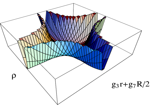
Figure 3: The potential

Given this understanding of the system’s motion, exciting the twisted sector further should result in the oscillations being large enough to effect a branch change when the system reaches the hub of the cross shaped potential . This corresponds to the D3-brane dissolving onto the D7 stack upon collision and does indeed occur as shown by the numerical results in figure 4. In this example the D3-brane is later re-emitted. The reason for this and the details of the late time behaviour shown in these plots will be discussed in detail later. For now we simply note that a small instanton transition has occurred (although the instanton has not monotonically smoothed out to some final size).

Figure 4: A sequence of two small instanton transitions: a D3-brane is captured but later emitted. As before time is plotted on a log scale.

Next we can ask what happens when we start with an initially dissolved D3-brane (i.e. with non-zero $\rho$) and allow it to evolve. If the D-branes are all initially coincident and stationary, then they will remain so for all time; again the relevant fields can be consistently truncated from the system by giving them these initial conditions. One then has a scalar field evolving in a quartic potential and one may ask if the system inflates. Alas, the answer is not to any appreciable degree. This is because the quartic potential has prefactors that go as inverse powers of the sizes of the compact spaces. The potential thus has two effects: it drives these moduli to large values and it drives the twisted states to small vevs. The former effect occurs so quickly due to the exponential nature of the relevant field dependence that very little inflation can occur because the potential for the twisted fields flattens out very quickly. This problem could perhaps be solved by employing some stabilisation mechanism to fix the relevant metric moduli fields. The potential would then still have various problems however as large initial field values would be required to obtain the requisite number of e-foldings, although such objections may be resolvable in various ways. These are problems which are familiar in traditional chaotic inflation [34].

Figure 5: Hubble damped oscillations of a dissolved D3-brane and the resulting (lack of) acceleration.

Finally if we begin with non-zero $\rho$ and also slightly excite the brane separation modulus the situation is very different. Indeed we find the reverse of the initially separated but excited D-branes; we would expect large enough excitations of the brane separation to cause a branch change when the system reaches the hub of the cross shaped potential. Such a branch change would correspond to the instanton being emitted as a D3-brane from the D7-brane stack. As the plots in figure 6 clearly show, the D3-brane can indeed be emitted in this manner.

Figure 6: Emission of a slightly excited dissolved D3-brane.

Multiple D7-branes

The previous discussion can be extended to consider multiple D7-brane stacks. Consider beginning with a single stack of 4 D7-branes beginning with a gauge group of $U(4)$. Keeping the previous truncation but with the division

$$C^{7}=\left(\begin{array}[]{cc}Re^{i\psi}\frac{1}{2}\mathbf{I}_{2}&\mathbf{0}\\ \mathbf{0}&R_{2}e^{i\psi_{2}}\frac{1}{2}\mathbf{I}_{2}\end{array}\right),$$ (29)

the four component twisted states in the ADHM truncation take the form

$$A_{\alpha} = (\rho(-i\theta_{3}+\theta_{4}),\,\rho(-i\theta_{1}-\theta_{2}),\,\rho_{2}(-i\varphi_{3}+\varphi_{4}),\,\rho_{2}(-i\varphi_{1}-\varphi_{2}))$$

$$B^{\alpha} = (\rho(i\theta_{1}+\theta_{2}),\,\rho(-i\theta_{3}+\theta_{4}),\,\rho_{2}(i\varphi_{1}+\varphi_{2}),\,\rho_{2}(-i\varphi_{3}+\varphi_{4})).$$ (30)

The system now describes two stacks of D7-branes whose positions in the transverse space are given by $R,\,R_{2}$. When $R\neq R_{2}$, the D7 gauge group is broken to $U(2)\times U(2)$, and the parameters $\rho$ and $\rho_{2}$ describe two orthogonal small instanton transitions with the D3-brane dissolving on either of the two D7-branes. With the definitions

$$Re\{S\} = e^{\phi}+\frac{1}{2}(R^{2}+R_{2}^{2})$$

$$Re\{T\} = e^{\beta}+\frac{1}{2}(\rho^{2}+\rho_{2}^{2})$$

$$Re\{T_{3}\} = e^{\beta_{3}}+\frac{1}{2}r^{2}$$ (31)

the action and equations of motion are extended in the obvious way.

There are two interesting types of behaviour that can be observed in this extended system. The first (and possibly less surprising) is that the D3-brane can be emitted from one D7-brane and captured by the second, and indeed this can happen a number of times before Hubble damping sets in. An example is shown in figure 7. In this case (as seen in the $R-R_{2}$ figure) the D7-branes are, in the region shown, essentially undergoing the free-field evolution of figure 1, and in fact the motion is just part of the typical ‘s-curve’. This is because the $g_{7}$ gauge coupling has deliberately been chosen to be quite small in order to decouple their motion from the D3-brane. The latter is evidently “stuck” on one of the D7 stacks for long periods while $\rho$ or $\rho_{2}$ are non-zero, before being transmitted between them on relatively short timescales when $\rho$ or $\rho_{2}$ pass through zero. The second type of behaviour is less obvious but actually more commonplace: if both $\rho$ and $\rho_{2}$ are slightly excited initially, then their subsequent oscillations cause the D7-branes to oscillate about each other, due to the time-averaged $\rho$ and $\rho_{2}$ oscillations giving an effective potential for the separation $R-R_{2}$. An example of this sort of behaviour is shown in figure 8 where the D7-brane displacement goes through zero where the gauge symmetry is enhanced to $U(4).$ Naturally at this point the D3-branes find it easiest to transfer between D7-branes. Note that the timescale for D7-brane attraction is exponentially longer than that for $\rho$ and $\rho_{2}$ oscillations, which in turn is exponentially longer than the timescale for D3 oscillations. The timescales for these oscillations are chiefly determined by the $g_{3},g_{7}$ couplings and the initial displacements. Whether the D7-branes recombine to give an enhanced $U(4)$ symmetry before the Hubble damping sets in depends on all these factors, but the generic behaviour is clearly that all the fields, including the D7 stacks, oscillate around the single symmetric point where $R=R_{2}$ and all the other fields are zero. (We consistently truncated various light states in the description of the physics here in order to maintain clarity, so the discussion of this point is somewhat qualitative.)

Figure 7: D3 “ping-pong”: a D3 being transferred back and forth between D7-brane stacks.

Figure 8: Two D7-branes being attracted by coupled excited small instantons. Note that here the D3-brane is stuck on the D7-brane stack with position $R$ for most of the evolution, but eventually begins to oscillate freely between them.

Chaotic behaviour and Lyapunov exponents

We have seen that small instanton transitions can indeed dynamically occur in phenomenological string settings, but we have found that the collision of a D3-brane with a D7 stack does not per se guarantee that such a transition will take place and even if it does the behaviour does not correspond to the smooth monotonic expansion of a dissolved D3-brane that might naively have been expected. Likewise the emission of a D3-brane from the D7 stack is not guaranteed when an instanton shrinks to zero size and, even if a small instanton transition does occur, it does not typically result in the newly created extended object escaping to infinity.

The final state of the system is in fact strongly dependent upon the initial conditions. In particular the degree of initial excitation of the twisted sector and D-brane separation moduli is the dominant factor in deciding what qualitative dynamical behaviour the system will exhibit. If both the instanton size and D-brane separation moduli are initially fairly excited, the system’s final state tends to be described by unpredictable chaotic oscillations about the small instanton transition point. The physical origin of this oscillatory behaviour is due to the potential being dominated by a term proportional to $\rho^{2}(g_{3}r+\frac{g_{7}}{2}R)^{2}$ in the vicinity of the transition point. Thus an expectation value for $\rho$ results in an effective mass term for the D-brane separation and vice versa. Small oscillations of $\rho$ , for example, then result in a time varying mass term for the D-brane separation modulus. The separation degree of freedom then oscillates in this time dependent potential well which in turn causes a contribution to the effective potential seen by the twisted sector, and so on.

The chaotic nature of the resulting oscillations should come as no surprise in a non-linear system such as this. Indeed the system with canonical kinetic terms in two fields $X$ and $Y$, with an $X^{2}Y^{2}$ potential is a well known partially chaotic system that has been studied in some depth [35, 37, 36]. This system (which we refer to as the ’$XY$ system’) is coincident with ours in the limit where the $\rho^{4}$ term in our potential is negligible and in the limit where the dynamics of the metric moduli and dilaton are associated with timescales much longer than those governing the oscillations we have been describing. The $XY$ system in fact exhibits chaotic behaviour for the vast majority of its possible initial conditions. Thus we expect that for a large class of initial conditions our system will also exhibit chaotic oscillatory behaviour with the oscillations tending to decay at late times due to Hubble damping.

That our system is truly chaotic can be confirmed by calculating the relevant Lyapunov exponents. If one of these exponents has a positive real part when the system appears to be unpredictable then the behaviour is truly chaotic in the sense that adjacent trajectories in phase space diverge exponentially. Plots of the real part of the maximal Lyapunov exponent $\Lambda_{max}$ can be found in the figures. It should be noted that the inverse Lyapunov exponents also contain information about timescales. For example, in figure 2 the Lyapunov exponent is non-zero but the behaviour appears to be quite predictable in the plot because the timescale $1/\Lambda_{max}\sim 10^{4}$ is comparable in size with the total time of the evolution shown. By contrast figure 4 is unpredictable because $1/\Lambda_{max}\sim 30$ is very short on the timescale of the plot. Note that the calculation of the Lyapunov exponents took into account all of the fields, including the compactification moduli and the dilaton, and so the effect of Hubble damping on the chaotic behaviour is already included in the plots. The behaviour is usually (but not always) tending to small Lyapunov exponents at large times.

An additional feature of the evolutions we can clearly see is that Hubble damping causes the “matter” fields $r,\rho,R$ to sample a surface in phase space that is shrinking as energy is Hubble damped away. This effect is not completely obvious as it depends on how fast the potential (which is dependent on for example $\beta$) is flattening out, but we found no counterexamples. One should also bear in mind though that, as is well known from previous studies [29, 30], the motion of the brane position moduli tends to freeze asymptotically (for sufficiently small excitations of the twisted fields) due to the cosmological evolution of $\alpha,\beta,\beta_{3}$, and it is not clear in any particular case which effect will dominate.

Of course in the chaotic regimes (i.e. where the inverse Lyapunov exponent is shorter than the timescales of interest) it is impossible to predict when the system will be in the Higgs or Coulomb branch (-like) phase, but at late times we see that the system tends to the point where the maximum number of light states occurs. This behaviour has a passing resemblance to the attraction to “extra species points” noted in ref.[38] although, since in that case the effect was quantum mechanical whereas here it is purely classical, it actually has more in common with the earlier results presented in refs.[39, 40, 41, 42]. We comment further on these similarities in the discussion.

5 Discussion

The behaviour we have described here is formally similar to other systems in string cosmology, particularly those where extra light states appear as a consequence of the evolution. A comparison can be drawn for example with the results of refs.[39, 40, 41, 42]. The system in those cases involved flop and conifold transitions in both string and $M$-theory compactifications. We would expect chaotic dynamics to be exhibited by these systems for appropriate ranges of initial conditions. Indeed indications of chaotic oscillations are evident in the plots of ref.[42].

As we noted in the previous section the behaviour is also qualitatively similar to that found in ref. [38]. In that work it was argued that systems which have a point where the number of light species is enhanced, a so-called “enhanced species point” (ESP), will experience damping due to quantum mechanical production of the light states every time they pass through these ESPs. In our case the ESP is the small instanton transition point, where the D3-brane is undissolved (i.e. $\rho=0$) but lying on top of the D7-brane. In fact this type of quantum mechanical effect will occur in our system as well. The states in question are precisely the open string ’twisted’ states stretching from D3 to D7-brane: on each pass through the ESP such states are produced and the energy required to stretch them puts a brake on the motion of the D3-brane with respect to the D7-brane [38, 43]. However at weak coupling and low velocities such effects are subdominant, with the evolution being essentially classical. What we can conclude from the present discussion is that even classically the D3/D7 system is driven to the ESP. A similar argument applies in systems with initially separated D7-branes. In that case the system is not only driven to the small instanton transition point, but the D7-branes are themselves attracted to each other and hence enhanced gauge symmetry as well. Along with this conclusion for the D3/D7 system, comes an important implication for model building in intersecting branes; since recombination transitions are T-dual (in a generic sense) to D3/D7 systems, it seems that such systems, if they have a period of unconstrained cosmological evolution, will naturally end up maximizing the number of light chiral states and gauge symmetries consistent with the topology of the initial configuration.

The fact that we obtain the chaotic behaviour described above for a very large range of initial conditions has significant implications for the cosmology of D-brane models. For example consider what the dynamics shown in figure 4 implies for the cosmology of the early Universe in a situation where the temperature in the Universe is negligible when compared to the energies involved in our numerical solutions. The $\rho$ and D-brane separation spend long periods of time being essentially unexcited followed by periods where they oscillate considerably. This corresponds to a series of moduli driven gauge symmetry changing phase transitions [44, 32] in which the gauge group is in turns enhanced and then reduced in rank. The mass scale of gauge symmetry breaking in the Higgs phase decreases with time and eventually goes to zero as the system settles down at the symmetric point. Such a sequence of phase transitions has not to our knowledge been considered in cosmology, but in our analysis we see that it is in fact quite typical; the usual picture in which the Universe undergoes sequential reduction of gauge symmetry in a series of phase transitions is not by any means universal in D-brane systems.

There are in addition many discussions of inflationary models involving D-branes. Refs.[45, 46, 47] specifically concerned D3/D7-brane systems and invoked various mechanisms for giving the slow-roll potential; for example in ref.[45], fluxes give a logarithmic potential in the Coulomb branch which causes inflation. (In a dual system the potential in question can be put down to the presence of non-zero brane angles corresponding to non-zero Fayet-Iliopoulos terms; the resulting model is known as “P-term” inflation [48].) The D3-brane rolls towards the D7-brane and dissolves on it, the dissolution playing the role of the “waterfall” stage of hybrid inflation. Our discussion is relevant to the dynamics of this type of phase transition. Indeed one interesting possibility is an explanation for the starting configuration. For the scenario to work one requires a sufficiently damped (i.e. with kinetic energy negligible compared to potential energy in order to satisfy the slow-roll conditions) D3-brane sitting out along the potential. The natural question to ask is how it got there. Here we have seen that it is quite natural for the D3-brane to have been emitted from a neighbouring D7-brane. Also in this context the production of multiple stages of inflation seems likely. Therefore it would be interesting to repeat the analysis for that case. The expectation is that once the flat directions are lifted (to generate inflation) the system will behave much as described in ref.[49]: chaotic behaviour will occur when the energy is higher than the barriers in the potential. There could be various interesting consequences such as for example enhanced production of defects such as cosmic strings. This is intimately related to the presence of chaos: inflation aims to solve the defect problem by exponentially suppressing variation in field values, but chaos makes the evolution exponentially sensitive to initial conditions.

6 Conclusion

In this paper we have described in microscopic detail the cosmological dynamics associated with small instanton (and brane recombination) transitions in type II string theory for the first time. We have seen that the naive picture of a D3-brane colliding with a D7 stack and becoming an instanton which monotonically increases in size with time is not in fact correct. Instead if such a phase transition does occur it tends to be chaotic with unpredictable oscillations about the point of transition. This results in various unusual types of behaviour. For example fairly generic initial conditions result in a sequence of symmetry breaking and restoring phase transitions, and hence a fluctuation of the low energy gauge group. At late times the system tends to points with enhanced numbers of light states, where the D3-branes are stuck on the D7-branes, as has been argued for in different contexts in the past. We also observe that at late times the D3-branes can sporadically jump between the different D7 stacks.

All of this behaviour could have significant implications for early Universe cosmology and for D-brane model building in general. A typical supersymmetric phenomenological construction consists of a number of separated D3 and D7-branes. Intuitively one imagines that, before all the moduli are (presumably) stabilised, the D-branes smoothly “glide about” in near BPS configurations; the present analysis shows that their behaviour is in fact more interesting and rather more complicated.

Acknowledgements

We thank D.Tong and V.V.Khoze for useful discussions. J. G. is supported by PPARC.

7 Appendix A: Equations of Motion

We present in this appendix the equations of motion which follow from the action in eq.(24) and the metric ansatz $ds^{2}=-dt^{2}+e^{2\alpha}d\vec{x}^{2}$. All fields and the metric function $\alpha$ are taken to be functions of $t$ only and derivatives with respect to this coordinate are denoted by a prime.

$$(12\alpha^{\prime}e^{3\alpha})^{\prime} = 3e^{3\alpha}\left[\frac{3}{16}g_{7}^{2}\rho^{4}e^{-2\beta-\beta_{3}}+\rho^{2}(g_{3}r+g_{7}\frac{R}{2})^{2}e^{-\phi-\beta-\beta_{3}}\right]$$

$$(-e^{3\alpha}\beta^{\prime})^{\prime} = e^{3\alpha}\left[\frac{1}{2}e^{-\beta}\rho^{\prime 2}-\frac{3}{16}g_{7}^{2}\rho^{4}e^{-2\beta-\beta_{3}}-\frac{1}{2}\rho^{2}(g_{3}r+g_{7}\frac{R}{2})^{2}e^{-\phi-\beta-\beta_{3}}\right]$$

$$(-e^{3\alpha}\frac{\phi^{\prime}}{2})^{\prime} = e^{3\alpha}\left[\frac{1}{2}e^{-\phi}R^{\prime 2}-\frac{1}{2}\rho^{2}(g_{3}r+g_{7}\frac{R}{2})^{2}e^{-\phi-\beta-\beta_{3}}\right]$$

$$(-e^{3\alpha}\frac{\beta_{3}^{\prime}}{2})^{\prime} = e^{3\alpha}\left[\frac{1}{2}e^{-\beta_{3}}r^{\prime 2}-\frac{3}{32}g_{7}^{2}\rho^{4}e^{-2\beta-\beta_{3}}-\frac{1}{2}\rho^{2}(g_{3}r+g_{7}\frac{R}{2})^{2}e^{-\phi-\beta-\beta_{3}}\right]$$

$$(-e^{3\alpha-\beta_{3}}r^{\prime})^{\prime} = e^{3\alpha}\left[g_{3}(g_{3}r+g_{7}\frac{R}{2})\rho^{2}e^{-\phi-\beta-\beta_{3}}\right]$$

$$(-e^{3\alpha-\phi}R^{\prime})^{\prime} = e^{3\alpha}\left[\frac{g_{7}}{2}(g_{3}r+g_{7}\frac{R}{2})\rho^{2}e^{-\phi-\beta-\beta_{3}}\right]$$

$$(-e^{3\alpha-\beta}\rho^{\prime})^{\prime} = e^{3\alpha}\left[\frac{3}{8}g_{7}^{2}\rho^{3}e^{-2\beta-\beta_{3}}+(g_{3}r+g_{7}\frac{R}{2})^{2}\rho e^{-\phi-\beta-\beta_{3}}\right].$$

In addition we obtain the following Hamiltonian constraint for the system:

$$6\alpha^{\prime 2}=\frac{1}{4}\phi^{\prime 2}+\frac{1}{2}e^{-\phi}R^{\prime 2}+\frac{1}{4}\beta_{3}^{\prime 2}+\frac{1}{2}\beta^{\prime 2}+\frac{1}{2}e^{-\beta}\rho^{\prime 2}+\frac{3}{32}g_{7}^{2}\rho^{4}e^{-2\beta-\beta_{3}}+(g_{3}r+g_{7}\frac{R}{2})^{2}\frac{1}{2}\rho^{2}e^{-\phi-\beta-\beta_{3}}\,.$$

It is these equations that are solved in the text, analytically for $\rho=0$ and numerically in other cases.

References

- [1] E. Witten, “Small Instantons in String Theory,” Nucl. Phys. B 460 (1996) 541 [arXiv:hep-th/9511030].
- [2] O. J. Ganor and A. Hanany, “Small Instantons and Tensionless Non-critical Strings,” Nucl. Phys. B 474 (1996) 122 [arXiv:hep-th/9602120]; E. Buchbinder, R. Donagi and B. A. Ovrut, JHEP 0206, 054 (2002) [arXiv:hep-th/0202084].
- [3] M. R. Douglas, “Branes within branes,” arXiv:hep-th/9512077; M. R. Douglas, “Gauge Fields and D-branes,” J. Geom. Phys. 28 (1998) 255 [arXiv:hep-th/9604198].
- [4] R. Blumenhagen, L. Goerlich, B. Kors and D. Lust, “Noncommutative compactifications of type I strings on tori with magnetic background flux,” JHEP 0010, 006 (2000) [arXiv:hep-th/0007024]; R. Blumenhagen, L. Goerlich, B. Kors and D. Lust, “Magnetic flux in toroidal type I compactifications,” Fortsch. Phys. 49, 591 (2001) [arXiv:hep-th/0010198]; M. Cvetic, G. Shiu and A. M. Uranga, “Three-family supersymmetric standard like models from intersecting brane worlds,” Phys. Rev. Lett. 87, 201801 (2001) [arXiv:hep-th/0107143].
- [5] for later references see R. Blumenhagen, M. Cvetic, P. Langacker and G. Shiu, “Toward realistic intersecting D-brane models,” arXiv:hep-th/0502005.
- [6] G. Aldazabal, L. E. Ibanez and F. Quevedo, “Standard-like models with broken supersymmetry from type I string vacua,” JHEP 0001, 031 (2000) [arXiv:hep-th/9909172]; G. Aldazabal, L. E. Ibanez and F. Quevedo, “A D-brane alternative to the MSSM,” JHEP 0002, 015 (2000) [arXiv:hep-ph/0001083]; G. Aldazabal, L. E. Ibanez, F. Quevedo and A. M. Uranga, “D-branes at singularities: A bottom-up approach to the string embedding of the standard model,” JHEP 0008, 002 (2000) [arXiv:hep-th/0005067]; D. Bailin, G. V. Kraniotis and A. Love, “Supersymmetric standard models on D-branes,” Phys. Lett. B 502, 209 (2001) [arXiv:hep-th/0011289]. D. Bailin and A. Love, “Non-minimal Higgs content in standard-like models from D-branes at a Z(N) singularity,” Phys. Lett. B 598, 83 (2004) [arXiv:hep-th/0406031];
- [7] G. Aldazabal, S. Franco, L. E. Ibanez, R. Rabadan and A. M. Uranga, “D = 4 chiral string compactifications from intersecting branes,” J. Math. Phys. 42 (2001) 3103 [arXiv:hep-th/0011073]; G. Aldazabal, S. Franco, L. E. Ibanez, R. Rabadan and A. M. Uranga, “Intersecting brane worlds,” JHEP 0102 (2001) 047 [arXiv:hep-ph/0011132]; M.Cvetic, G.Shiu and A.M.Uranga, “Chiral four-dimensional N = 1 supersymmetric type IIA orientifolds from intersecting D6-branes,” Nucl. Phys. B 615 (2001) 3 [arXiv:hep-th/0107166].
- [8] D. Berenstein, V. Jejjala and R. G. Leigh, “The standard model on a D-brane,” Phys. Rev. Lett. 88, 071602 (2002) [arXiv:hep-ph/0105042]; L. E. Ibanez, F. Marchesano and R. Rabadan, “Getting just the standard model at intersecting branes,” JHEP 0111, 002 (2001) [arXiv:hep-th/0105155]; R. Blumenhagen, B. Kors, D. Lust and T. Ott, “The standard model from stable intersecting brane world orbifolds,” Nucl. Phys. B 616, 3 (2001) [arXiv:hep-th/0107138]; D. Cremades, L. E. Ibanez and F. Marchesano, “Intersecting brane models of particle physics and the Higgs mechanism,” JHEP 0207, 022 (2002) [arXiv:hep-th/0203160]; D. Cremades, L. E. Ibanez and F. Marchesano, “Standard model at intersecting D5-branes: Lowering the string scale,” Nucl. Phys. B 643, 93 (2002) [arXiv:hep-th/0205074].
- [9] For a review see C. Angelantonj and A. Sagnotti, “Open strings,” Phys. Rept. 371, 1 (2002) [Erratum-ibid. 376, 339 (2003)] [arXiv:hep-th/0204089].
- [10] B. S. Acharya, “M theory, Joyce orbifolds and super Yang-Mills,” Adv. Theor. Math. Phys. 3 (1999) 227 [arXiv:hep-th/9812205].
- [11] B. S. Acharya, “On realising N = 1 super Yang-Mills in M theory,” arXiv:hep-th/0011089.
- [12] B. Acharya and E. Witten, “Chiral fermions from manifolds of G(2) holonomy,” arXiv:hep-th/0109152.
- [13] M. Atiyah and E. Witten, “M-theory dynamics on a manifold of G(2) holonomy,” Adv. Theor. Math. Phys. 6 (2003) 1 [arXiv:hep-th/0107177].
- [14] E. Witten, “Anomaly cancellation on G(2) manifolds,” arXiv:hep-th/0108165.
- [15] See J. Polchinski, “String theory. Vol. 2: Superstring theory and beyond.” (CUP 1998), and references therein.
- [16] See J. Erdmenger, Z. Guralnik, R. Helling and I. Kirsch, “A world-volume perspective on the recombination of intersecting branes,” JHEP 0404 (2004) 064 [arXiv:hep-th/0309043] for some related work.
- [17] For a review see the early sections of N. Dorey, T. J. Hollowood, V. V. Khoze and M. P. Mattis, “The calculus of many instantons,” Phys. Rept. 371 (2002) 231 [arXiv:hep-th/0206063].
- [18] P. J. Braam and P. van Baal, “Nahm’s Transformation For Instantons,” Commun. Math. Phys. 122 (1989) 267.
- [19] P. van Baal, “Instanton moduli for T(3) x R,” Nucl. Phys. Proc. Suppl. 49 (1996) 238 [arXiv:hep-th/9512223].
- [20] L. E. Ibanez, C. Munoz and S. Rigolin, “Aspects of type I string phenomenology,” Nucl. Phys. B 553 (1999) 43 [arXiv:hep-ph/9812397].
- [21] M. Grana, T. W.Grimm, H. Jockers and J. Louis, “Soft supersymmetry breaking in Calabi-Yau orientifolds with D-branes and fluxes,” Nucl. Phys. B 690 (2004) 21 [arXiv:hep-th/0312232].
- [22] D. Lust, P. Mayr, R. Richter and S. Stieberger, “Scattering of gauge, matter, and moduli fields from intersecting branes,” Nucl. Phys. B 696 (2004) 205 [arXiv:hep-th/0404134].
- [23] D. Lust, S. Reffert and S. Stieberger, “Flux-induced soft supersymmetry breaking in chiral type IIb orientifolds with D3/D7-branes,” Nucl. Phys. B 706 (2005) 3 [arXiv:hep-th/0406092].
- [24] H. Jockers and J. Louis, “The effective action of D7-branes in N = 1 Calabi-Yau orientifolds,” Nucl. Phys. B 705 (2005) 167 [arXiv:hep-th/0409098].
- [25] H. Jockers and J. Louis, “D-terms and F-terms from D7-brane fluxes,” arXiv:hep-th/0502059.
- [26] M. Mueller, “Rolling Radii And A Time Dependent Dilaton,” Nucl. Phys. B 337 (1990) 37.
- [27] M. Brandle, A. Lukas and B. A. Ovrut, “Heterotic M-theory cosmology in four and five dimensions,” Phys. Rev. D 63 (2001) 026003 [arXiv:hep-th/0003256].
- [28] E. J. Copeland, A. Lahiri and D. Wands, “Low-energy effective string cosmology,” Phys. Rev. D 50 (1994) 4868 [arXiv:hep-th/9406216].
- [29] J. E. Lidsey, D. Wands and E. J. Copeland, “Superstring cosmology,” Phys. Rept. 337 (2000) 343 [arXiv:hep-th/9909061].
- [30] E. J. Copeland, J. Gray and A. Lukas, “Moving five-branes in low-energy heterotic M-theory,” Phys. Rev. D 64 (2001) 126003 [arXiv:hep-th/0106285].
- [31] J. Gray, A. Lukas and G. I. Probert, “Gauge five brane dynamics and small instanton transitions in heterotic models,” Phys. Rev. D 69 (2004) 126003 [arXiv:hep-th/0312111].
- [32] J. Gray, “An explicit example of a moduli driven phase transition in heterotic models,” arXiv:hep-th/0406241.
- [33] M. Gasperini and G. Veneziano, “The pre-big bang scenario in string cosmology,” Phys. Rept. 373, 1 (2003) [arXiv:hep-th/0207130]; J. Khoury, B. A. Ovrut, P. J. Steinhardt and N. Turok, “The ekpyrotic universe: Colliding branes and the origin of the hot big bang,” Phys. Rev. D 64, 123522 (2001) [arXiv:hep-th/0103239].
- [34] A. D. Linde, “Chaotic Inflation,” Phys. Lett. B 129, 177 (1983).
- [35] W-H Steeb, C. M. Villet and A. Kunick, “Chaotic behaviour of a Hamiltonian with a quartic potential.” J. Phys. A: Math. Gen. (1985) 3269-3273.
- [36] P. Dahlqvist and G. Russberg, “Existence of Stable Orbits in the Potential.” Phys. Rev. Lett. 65 (1990) 2837-2838.
- [37] M. L. A. Nip, J. A. Tuszynski, M. Otwinowski and J. M. Dixon, “Search for regular orbits in the potential problem.” J. Phys. A: Math. Gen. 25 (1992) 5553-5562.
- [38] L. Kofman, A. Linde, X. Liu, A. Maloney, L. McAllister and E. Silverstein, “Beauty is attractive: Moduli trapping at enhanced symmetry points,” JHEP 0405 (2004) 030 [arXiv:hep-th/0403001].
- [39] M. Brandle and A. Lukas, “Flop transitions in M-theory cosmology,” Phys. Rev. D 68 (2003) 024030 [arXiv:hep-th/0212263].
- [40] L. Jarv, T. Mohaupt and F. Saueressig, “M-theory cosmologies from singular Calabi-Yau compactifications,” JCAP 0402 (2004) 012 [arXiv:hep-th/0310174].
- [41] T. Mohaupt and F. Saueressig, “Dynamical conifold transitions and moduli trapping in M-theory cosmology,” JCAP 0501 (2005) 006 [arXiv:hep-th/0410273].
- [42] A. Lukas, E. Palti and P. M. Saffin, “Type IIB conifold transitions in cosmology,” Phys. Rev. D 71 (2005) 066001 [arXiv:hep-th/0411033].
- [43] C. Bachas, “D-brane dynamics,” Phys. Lett. B 374, (1996) 37, [arXiv:hep-th/9511043]; M. R. Douglas, D. Kabat, P. Pouliot and S. H. Shenker, “D-branes and short distances in string theory,” Nucl. Phys. B 485, (1997) 85, [arXiv:hep-th/9608024]; E. Silverstein and D. Tong, “Scalar speed limits and cosmology: Acceleration from D-cceleration,” Phys. Rev. D 70, 103505 (2004) [arXiv:hep-th/0310221]; Consult C. P. Bachas, “Lectures on D-branes,” arXiv:hep-th/9806199;
- [44] M. Bastero-Gil, E. J. Copeland, J. Gray, A. Lukas and M. Plumacher, “Baryogenesis by brane-collision,” Phys. Rev. D 66 (2002) 066005 [arXiv:hep-th/0201040].
- [45] K. Dasgupta, C. Herdeiro, S. Hirano and R. Kallosh, “D3/D7 inflationary model and M-theory,” Phys. Rev. D 65, 126002 (2002) [arXiv:hep-th/0203019].
- [46] K. Dasgupta, J. P. Hsu, R. Kallosh, A. Linde and M. Zagermann, “D3/D7 brane inflation and semilocal strings,” JHEP 0408, 030 (2004) [arXiv:hep-th/0405247].
- [47] F. Koyama, Y. Tachikawa and T. Watari, “Supergravity analysis of hybrid inflation model from D3-D7 system,” Phys. Rev. D 69, 106001 (2004) [Erratum-ibid. D 70, 129907 (2004)] [arXiv:hep-th/0311191]; S. E. Shandera, “Slow roll in brane inflation,” arXiv:hep-th/0412077.
- [48] R. Kallosh and A. Linde, “P-term, D-term and F-term inflation,” JCAP 0310, 008 (2003) [arXiv:hep-th/0306058].
- [49] R. Easther and K. I. Maeda, “Chaotic dynamics and two-field inflation,” Class. Quant. Grav. 16, 1637 (1999) [arXiv:gr-qc/9711035].