Shift Symmetry and Inflation in Supergravity

Abstract

We consider models of inflation in supergravity with a shift symmetry. We focus on models with one moduli and one inflaton field. The presence of this symmetry guarantees the existence of a flat direction for the inflaton field. Mildly breaking the shift symmetry using a superpotential which depends not only on the moduli but also on the inflaton field allows one to lift the inflaton flat direction. Along the inflaton direction, the $\eta$-problem is alleviated. Combining the KKLT mechanism for moduli stabilization and a shift symmetry breaking superpotential of the chaotic inflation type, we find models reminiscent of “mutated hybrid inflation” where the inflationary trajectory is curved in the moduli–inflaton plane. We analyze the phenomenology of these models and stress their differences with both chaotic and hybrid inflation.

Keywords : Inflation, Supergravity, Superstring Theory, Cosmology

I Introduction

The recent observations of the Cosmic Microwave Background (CMB) fluctuations wmap give a strong hint in favor of an early period of inflation inflation in the history of the Universe. Inflation is an attractive scenario as it allows us to avoid the difficulties which plague the standard hot big bang theory, e.g. the flatness and the horizon problems. Moreover, when combined with quantum mechanics, inflation can also give rise to a satisfactory model for structure formation, see Refs. pert . As a matter of fact, inflation implies that the power spectrum of the cosmological perturbations should be (almost) scale invariant pert , a prediction which has been known for a long time to be in good agreement with the astrophysical data. In fact, the data are now so accurate that one can start probing the details of the inflationary scenario. For instance, the small deviation from scale invariance in the power spectrum predicted by inflation (for density perturbations and for gravitational waves) directly encodes the underlying high energy physics responsible for the phase of accelerated expansion slowroll implying that the model building issue for inflation is meaningful LR .

The above-mentioned observations and the endeavor to better understand space–like singularities like the big-bang have sparked a renewed interest in cosmological models based on string theory and/or supergravity cosmological . In this framework, alternatives to inflation have also been studied like, for instance, the pre big-bang scenario PBB or the ekpyrotic model ekp , but so far no scenario has been as successful as inflation. Hence, finding a satisfactory inflationary scenario from the most recent ideas in string theory is an important challenge stringinflation . In all these attempts, our universe is pictured as a moving brane embedded in a compactification space. The acceleration of the universe is caused by the motion of the brane Dvali . At the level of the four dimensional effective description obtained after compactification, the theory results in particular supergravity models. Then, in general, two main issues must be addressed in order to obtain a satisfactory scenario.

The first problem is to obtain a sufficiently flat potential. One of the crucial stumbling blocks of F–term inflation in supergravity is the presence of large ${\cal O}\left(H\right)$ corrections (where $H$ is the Hubble parameter during inflation) to the inflaton mass, which spoil the flatness of the inflaton potential. In order to lead to realistic models, the string–inspired scenarios for inflation must overcome this problem. Another highly conspicuous problem is the stabilization issue. In string inflation, the 10–dimensional type IIB theory is compactified on a Calabi-Yau manifold. Calabi-Yau compactifications lead to two types of moduli fields describing the Kähler and complex structure deformations. There is also another scalar degree of freedom originating from the 10–dimensional dilaton. Now all these moduli fields need to be stabilized in order to guarantee the flatness of the inflaton potential, i.e. no runaway behavior in the moduli directions.

Different solutions to the above-mentioned questions have been proposed. In particular, it has been noted recently that one can obtain flat enough potentials by requiring that a shift symmetry $\phi\to\phi+c$, where $c$ is a real constant, is a symmetry of the Kähler potential, later broken mildly. This is particularly natural within the low energy description of brane dynamics emerging from string theory Tye ; shift ; Hsu ; D3 ; koyama . On the other hand, for the stabilization question, the complex structure moduli and the dilaton can be generically stabilized when fluxes are turned on. This leaves only the Kähler moduli as flat directions. The Kähler moduli can be also stabilized once strong coupling effects, such as gaugino condensation, take place on a stack of $D7$ branes wrapped around a four-cycle in the Calabi-Yau variety. This leads to an ${\rm AdS}_{4}$ supergravity background. Now de Sitter space can be achieved by incorporating an anti $D3$ brane whose energy density makes the total energy density positive, this is the KKLT stabilization mechanism KKLT . It was then realized that the lifting of the vacuum energy can be performed in a supersymmetric way using Fayet–Iliopoulos terms Burgess2 . In supergravity, it has been recently argued that this mechanism is problematic as the Fayet–Iliopoulos terms of supergravity vanish in a supergravity vacuum nilles .

A first attempt to combine inflation with the KKLT mechanism was carried out in the KKLMMT paper, see Ref. KKLMMT . In this model, string inflation is obtained when a pair of $D3$-anti $D3$ branes is added to the configuration needed for the KKLT mechanism and described above. The anti $D3$ is naturally sitting on top of the other anti $D3$ branes, the distance between the $D3$ and anti $D3$ branes playing the role of the inflaton. The shift symmetry is explicitly broken by the non-perturbative superpotential leading to the stabilization of the Kähler moduli. The flat directions corresponding the free motion of a $D3$ brane in the Calabi-Yau space are then lifted in a strong manner. As a consequence, since the shift symmetry is absent, the corresponding inflationary model suffers from the $\eta$ problem. More precisely, it has been shown that the squared mass of the inflaton is $2H^{2}$ spoiling the flatness of the potential. This example is typical of the general flatness problem of supergravity potentials when no shift symmetry is present.

Subsequent papers have tried to overcome this problem by taking into account the shift symmetry while still relying on the KKLT mechanism for stabilizing the moduli fields. The first model Hsu to combine both aspects was based on an interesting type of configuration (different from the one envisaged in the KKLMMT paper) corresponding to $D7$ branes evolving in the background of a very heavy stack of $D3$ branes Hsu ; koyama ; D3 . In this case, one may consider the free motion of the $D7$ brane and the associated shift symmetry. The model realizes hybrid inflation in string inflation. The waterfall fields are represented by the charged open strings between the $D3$ and the $D7$ branes. When the distance between the branes is large enough, the configuration admits a flat direction which is lifted at one loop as in supersymmetric hybrid inflation hence giving a logarithmic slope to the potential in the inflaton direction. The presence of a flat direction is directly linked to the fact that the superpotential takes the form required to both preserve the shift symmetry and stabilize the Kähler moduli. For small distances between the branes, the waterfall fields condense and inflation ends.

Another possibility was studied in Refs. Tye . It consists in implementing the shift symmetry in the context of the original KKLMMT scenario, where inflation is obtained when a pair of $D3$-anti $D3$ branes is present. In fact, the shift symmetry is present initially in the Kähler potential. Imposing the shift symmetry invariance of the superpotential leads to a flat potential for the inflation. Inflation is then due to the small interaction potential between the $D3$ and the anti $D3$ brane. As in usual brane inflation this requires an adjustment of the brane–antibrane potential. In this context, it has been noticed that threshold corrections in string theory give rise to an explicitly shift symmetry breaking superpotential. As a consequence, the model suffers from the $\eta$-problem unless the stabilization of the complex structure moduli is fine-tuned. We will discuss this model (and compare it to what is achieved in the present article) where the non-perturbative superpotential responsible for the stabilization of the Kähler moduli is multiplicatively corrected by loop effects mac ; berg . Finally the shift symmetry is also instrumental in the race–track inflation model race .

Notice that combining the KKLT approach to stabilization and the shift symmetry in string theory requires the existence of isometries on Calabi–Yau threefolds as originally argued in Ref. shift for compactifications on $\mathbb{K}_{3}\times\mathbb{T}^{2}$. In the following, we will concentrate on supergravity issues only and use string motivations as a guideline only.

Combining the flatness of the F–term inflation potential in supergravity using the shift symmetry and the stabilization of moduli (in particular using the KKLT mechanism) is the aim of this paper. We will extract the main ingredients from the D3/D7 system in string theory and deal with its supergravity description exclusively. The two main new aspects of the model presented here are the following. Firstly, we will consider a case where the shift symmetry is initially present in both the Kähler and the superpotential before being mildly broken by an explicit inflaton dependence of the superpotential. In our case, the fact that the superpotential can depend on the inflaton field allows us to give a (small) slope to the potential already at the tree level without having to compute the quantum corrections. Notice that the shift symmetry breaking superpotential has coefficients constrained by the COsmic Background Explorer (COBE) normalization and must therefore be small. We also insist on obtaining the inflationary potential from a strict $N=1$ supergravity context. Secondly, we find that the end of inflation is due to the presence of the moduli field playing the role of a waterfall field. Contrary to the hybrid inflation case, the end of inflation is not triggered by extra fields representing the charged open strings between the branes. In fact, the name waterfall field is not very appropriate in our case since we will see that the effective inflationary model is reminiscent of mutated inflation and that inflation stops due to the violation of the slow-roll conditions and not by instability.

The outline of the paper is the following. In section II, we present the flatness problem in F–term supergravity inflation and discuss the realization of the shift symmetry as a Kähler transformation. The shift symmetry alleviates the flatness problem and leads to restrictions on the type of possible superpotentials. In section III, we give examples of chaotic inflation models with a shift symmetry broken by the superpotential. The model has problems such as runaway potentials. In Section IV, we then introduce what we call “mutated chaotic inflation” based on a chaotic inflation superpotential and for which the inflationary trajectories become curved. This model does not suffer from the $\eta$-problem and the moduli is stabilized. We give a thorough analysis of the inflationary parameter space. In particular, we find that the model is different from hybrid inflation. In section V, we combine the KKLT stabilization mechanism and a chaotic inflation superpotential. This gives another realization of mutated chaotic inflation. Then, we discuss various aspects of our results. Finally, in section VI we present our conclusions.

II Shift Symmetry in Supergravity

II.1 The $\eta$-problem

One of the stumbling blocks of F-term inflation in supergravity is the natural presence of ${\cal O}\left(H\right)$ corrections to the inflaton mass which would spoil the flatness of the potential (the so–called $\eta$-problem). Let us consider the Kähler potential for the inflaton of the form $K\left(\phi,\phi^{\dagger}\right)=\phi\phi^{\dagger}$ and its role in the scalar potential of supergravity

$$\exp\left[\kappa K\left(\phi,\phi^{\dagger}\right)\right]V_{\rm inf}\,,$$ (1)

where $V_{\rm inf}$ is the inflationary potential when neglecting the supergravity corrections and where $\kappa$ is defined by $\kappa\equiv 8\pi/m_{{}_{\mathrm{P}l}}^{2}$. Expanding the exponential leads to

$$\left[1+\kappa K\left(\phi,\phi^{\dagger}\right)+\cdots\right]V_{\rm inf}\,.$$ (2)

The first term leads to the inflation potential, while the second one leads to a term in $H^{2}\phi\phi^{\dagger}$ which spoils the flatness of the potential, i.e. the quantity

$$\frac{m_{\rm Pl}^{2}}{8\pi}\frac{1}{V}\frac{\partial^{2}V}{{\rm\partial}\phi^{2}}\,,$$ (3)

becomes of order one. However, one should also remark the following. The above parameter (the so-called $\eta$-parameter) is not the parameter which controls whether inflation is taking place or not. Indeed, strictly speaking, the condition $\ddot{a}>0$, where $a(t)$ is the Friedmann-Lemaître-Robertson-Walker scale factor, is equivalent to $\epsilon\equiv-\dot{H}/H^{2}<1$ or $m_{\rm Pl}^{2}/(16\pi V^{2})(\partial V/\partial\phi)^{2}<1$. When the $\eta$-parameter becomes of order one, we just have violation of the slow-roll conditions although, in principle, inflation could still proceed. Of course, one could argue, based on the well-known formula, $n_{{}_{\rm S}}-1\simeq 2\eta-6\epsilon$, that a parameter $\eta$ of order one would imply a scalar spectral index far from scale invariance, i.e. $|n_{{}_{\rm S}}-1|\gg 1$. Again, this conclusion is not rigorous because the previous formula is derived under the assumption that the slow-roll conditions are valid and, hence, not applicable when $\eta$ is large. In principle, one could imagine a situation where $\eta$ is large but where inflation proceeds and leads to an almost scale-invariant spectrum. Admittedly, this is probably not the most generic situation but this is possible in principle; for interesting recent remarks on the $\eta$ problem, see also Ref. kinney .

II.2 Shift symmetry

Let us now consider a typical ansatz, motivated by string inspired theories Hsu given by

$$K = -\frac{3}{\kappa}\ln\left[\kappa^{1/2}\left(\rho+\rho^{\dagger}\right)-\sigma\kappa{\cal K}\left(\phi,\phi^{\dagger}\right)\right]$$ (4)

$$+s{\cal G}\left(\phi,\phi^{\dagger}\right)\,,$$

$$W = W\left(\rho,\phi\right)\,,$$ (5)

where $\sigma=0,1$ and/or $s=0,1$ according to the situation we want to describe. In the above expression, the field $\rho$ is a moduli while $\phi$ represents the inflaton. When $\sigma=1$ and $s=0$, the Kähler potential describes the motion of a $D3$ brane within a Calabi-Yau manifold (we have only retained one of the possible six directions). In that case ${\cal K}\left(\phi,\phi^{\dagger}\right)$ is the Kähler potential on the Calabi-Yau manifold. For small arguments, one can expand ${\cal K}\left(\phi,\phi^{\dagger}\right)=\phi\phi^{\dagger}+\cdots$. Similarly when $\sigma=0$, ${\cal G}$ is also identified with the Kähler potential of the Calabi-Yau manifold and $\phi$ corresponds to the position of a $D7$ brane. These two cases will be exemplified later.

Let us come back to the issue of the shift symmetry $\phi\to\phi+c$ where $c$ is real which guarantees that the real part of the inflaton superfield is a flat direction. Following the above discussion, we focus on the Kähler potential

$$K=-\frac{3}{\kappa}\ln\left[\kappa^{1/2}(\rho+\rho^{\dagger})-\sigma\kappa\phi\phi^{\dagger}\right]+s\phi\phi^{\dagger}\,.$$ (6)

which follows from Eq. (4) in the small argument limit. Let us also remind that a Kähler transformation is a transformation which leaves the Lagrangian of a supergravity theory invariant. It is of the form

$$K(\rho,\phi) \to K(\rho,\phi)+\xi\left(\rho,\phi\right)+\xi^{\dagger}\left(\rho^{\dagger},\phi^{\dagger}\right)\,,$$ (7)

$$W(\rho,\phi) \to {\rm e}^{-\kappa\xi(\rho,\phi)}W(\rho,\phi)\,,$$ (8)

where $\xi$ is an arbitrary function. The shift symmetry, $\phi\to\phi+c$, can be viewed as a Kähler transformation provided the moduli field $\rho$ transforms in a specific way and the superpotential possesses a given form, namely

$$\rho \to \rho+\sigma c\kappa^{1/2}\phi+\sigma\kappa^{1/2}\frac{c^{2}}{2}\,,$$ (9)

$$W(\rho,\phi) = {\rm e}^{-s\kappa\phi^{2}/2}W\left(\rho-\sigma\kappa^{1/2}\frac{\phi^{2}}{2}\right)\,.$$ (10)

First of all, one can check that the quantities $\kappa^{1/2}\left(\rho+\rho^{\dagger}\right)-\sigma\kappa\phi\phi^{\dagger}$ and $\rho-\sigma\kappa^{1/2}\phi^{2}/2$ are invariant under the above transformation of the fields $\phi$ and $\rho$. Secondly, if the superpotential has the form given in Eq. (10), then the corresponding Kähler transformation is described by the function

$$\xi(\phi)=sc\phi+s\frac{c^{2}}{2}\,.$$ (11)

Therefore, if we want to implement the shift symmetry, one must restrict our considerations to models described by the Kähler potential given in Eq. (6) and superpotential given by Eq. (10).

This class of models can be simplified further (or transform to another form). Two ingredients are necessary. The first one is a Kähler transformation described by the function $\xi=-s\phi^{2}/2$ (this Kähler transformation has of course nothing to do with the other Kähler transformation considered before). In this case the Kähler potential and superpotential of the shift symmetry invariant model is equivalent to the one given by

$$K = -\frac{3}{\kappa}\ln\left[\kappa^{1/2}(\rho+\rho^{\dagger})-\sigma\kappa\phi\phi^{\dagger}\right]$$ (12)

$$-\frac{s}{2}\left(\phi-\phi^{\dagger}\right)^{2}\,,$$

$$W(\rho,\phi) = W\left(\rho-\sigma\kappa^{1/2}\frac{\phi^{2}}{2}\right)\,.$$ (13)

The second ingredient consists in changing variables in a holomorphic way (as required by supersymmetry) $\rho\to\rho-\sigma\kappa^{1/2}\phi^{2}/2$. In terms of the new variables, the Kähler potential becomes

$$K = -\frac{3}{\kappa}\ln\left[\kappa^{1/2}\left(\rho+\rho^{\dagger}\right)+\frac{\sigma}{2}\kappa\left(\phi-\phi^{\dagger}\right)^{2}\right]$$ (14)

$$-\frac{s}{2}\left(\phi-\phi^{\dagger}\right)^{2}\,,$$

$$W(\rho,\phi) = W(\rho)\,.$$ (15)

This representation guarantees that the inflaton field has a flat direction. This is the representation with ${\cal K}=-\sigma\left(\phi-\phi^{\dagger}\right)^{2}/2$ and ${\cal G}=-s\left(\phi-\phi^{\dagger}\right)^{2}/2$ in Eq. (4). The previous model does not immediately lead to inflation in the $\phi$ direction as the scalar potential is exactly flat along the real $\Re(\phi)$ direction due to the shift symmetry (but the potential could be lifted by quantum corrections). A large class of supergravity models with no $H^{2}$ corrections to the inflaton mass can be constructed by modifying the previous superpotential and including an explicit $\phi$ dependence which breaks the shift symmetry. Notice that the $H^{2}$ corrections will be absent as the Kähler potential is still shift symmetric. We now turn to the construction of such models.

III Inflation and Shift Symmetry

III.1 The scalar potential

Following the discussion of the previous section, we now generalize the class of models invariant under the shift symmetry and consider the Kähler potential given by (we remind that, in the present context, the field $\phi$ will be viewed as the inflaton while the field $\rho$ will represent a moduli)

$$K=-\frac{3}{\kappa}\ln\left[\kappa^{1/2}\left(\rho+\rho^{\dagger}\right)-\kappa{\cal K}\left(\phi-\phi^{\dagger}\right)\right]+{\cal G}\left(\phi-\phi^{\dagger}\right)\,$$ (16)

in such a way that the shift symmetry is explicitly present. In the above expression, ${\cal K}$ and ${\cal G}$ are arbitrary functions, the form of which is not specified at this stage. In order to calculate the corresponding potential, one must first evaluate the matrix $G_{A\bar{B}}$ defined by

$$G_{A\bar{B}}=\frac{\partial^{2}}{\partial\varphi^{A}\partial\left(\varphi^{B}\right)^{\dagger}}\left[\kappa K+\ln\left(\kappa^{3}\left|W\right|^{2}\right)\right]\,,$$ (17)

where $\varphi^{A}=\{\rho,\phi\}$ and where $W=W\left(\rho,\phi\right)$ is the superpotential which, as announced, explicitly depends on $\phi$. Explicitly, straightforward calculations lead to

$$G_{A\bar{B}}=\left\{\begin{matrix}\displaystyle 3\frac{\kappa}{\Delta^{2}}&\,\,\,\,\,&\displaystyle 3\frac{\kappa^{3/2}}{\Delta^{2}}\frac{\partial{\cal K}}{\partial\left(\phi-\phi^{\dagger}\right)}\cr\cr\displaystyle-3\frac{\kappa^{3/2}}{\Delta^{2}}\frac{\partial{\cal K}}{\partial\left(\phi-\phi^{\dagger}\right)}&\,\,\,\,\,&\displaystyle-3\frac{\kappa}{\Delta}\frac{\partial^{2}{\cal K}}{\partial\left(\phi-\phi^{\dagger}\right)^{2}}-3\frac{\kappa^{2}}{\Delta^{2}}\left[\frac{\partial{\cal K}}{\partial\left(\phi-\phi^{\dagger}\right)}\right]^{2}-\kappa\frac{\partial^{2}{\cal G}}{\partial\left(\phi-\phi^{\dagger}\right)^{2}}\end{matrix}\right\}\,,$$ (18)

where the quantity $\Delta$ is defined by $\Delta\equiv\kappa^{1/2}\left(\rho+\rho^{\dagger}\right)-\kappa{\cal K}\left(\phi-\phi^{\dagger}\right)$. These models are of the no-scale type with a cancellation of the $-3|W|^{2}$ term in the scalar potential $V={\rm e}^{G}\left(G^{A}G_{A}-3\right)/\kappa^{2}$ [we remind here that the function $G$ is given by $G\equiv\kappa K+\ln\left(\kappa^{3}|W|^{2}\right)$]. The potential reads

$${\rm e}^{-\kappa{\cal G}}V(\rho,\phi) = \frac{1}{3\Delta}\biggl{|}\frac{\partial W}{\partial\rho}\biggr{|}^{2}\times\left\{1+\frac{\kappa}{\Delta{\cal D}}\left[\frac{\partial{\cal K}}{\partial\left(\phi-\phi^{\dagger}\right)}\right]^{2}\right\}-\frac{1}{\Delta^{2}{\cal D}}\left|\frac{\partial W}{\partial\phi}\right|^{2}$$ (19)

$$-\frac{\kappa^{1/2}}{\Delta^{2}}\left(W\frac{\partial W^{\dagger}}{\partial\rho^{\dagger}}+W^{\dagger}\frac{\partial W}{\partial\rho}\right)\times\left[1-\frac{\kappa}{{\cal D}}\frac{\partial{\cal K}}{\partial\left(\phi-\phi^{\dagger}\right)}\frac{\partial{\cal G}}{\partial\left(\phi-\phi^{\dagger}\right)}\right]$$

$$+\frac{\kappa^{2}}{\Delta^{2}{\cal D}}\left[\frac{\partial{\cal G}}{\partial\left(\phi-\phi^{\dagger}\right)}\right]^{2}|W|^{2}-\frac{\kappa^{1/2}}{\Delta^{2}{\cal D}}\frac{\partial{\cal K}}{\partial\left(\phi-\phi^{\dagger}\right)}\left(\frac{\partial W}{\partial\rho}\frac{\partial W^{\dagger}}{\partial\phi^{\dagger}}-\frac{\partial W^{\dagger}}{\partial\rho^{\dagger}}\frac{\partial W}{\partial\phi}\right)$$

$$+\frac{\kappa}{\Delta^{2}{\cal D}}\frac{\partial{\cal G}}{\partial\left(\phi-\phi^{\dagger}\right)}\left(W^{\dagger}\frac{\partial W}{\partial\phi}-W\frac{\partial W^{\dagger}}{\partial\phi^{\dagger}}\right)\,,$$

where the coefficient ${\cal D}$ is defined by the following expression

$${\cal D}\equiv 3\frac{\partial^{2}{\cal K}}{\partial\left(\phi-\phi^{\dagger}\right)^{2}}+\Delta\frac{\partial^{2}{\cal G}}{\partial\left(\phi-\phi^{\dagger}\right)^{2}}\,.$$ (20)

Let us notice that, if the fields $\rho$ and $\phi$ are real and if the superpotential $W$ is also real when $\rho$ and $\phi$ are real, then the above expression can be simplified further since the last two terms cancel out. Moreover, if ${\cal G}=0$ and if the superpotential does not depend on the field $\phi$ but only on the moduli $\rho$ , then one recovers the expression (5.12) found in Ref. KKLMMT (which, therefore, appears to be a particular case of the most general formula established above), namely

$$V(\rho) = \frac{1}{3\Delta}\biggl{|}\frac{\partial W}{\partial\rho}\biggr{|}^{2}\times\left\{1+\frac{\kappa}{3\Delta}\left[\frac{\partial^{2}{\cal K}}{\partial\left(\phi-\phi^{\dagger}\right)^{2}}\right]^{-1}\times\left[\frac{\partial{\cal K}}{\partial\left(\phi-\phi^{\dagger}\right)}\right]^{2}\right\}-\frac{\kappa^{1/2}}{\Delta^{2}}\left(W\frac{\partial W^{\dagger}}{\partial\rho^{\dagger}}+W^{\dagger}\frac{\partial W}{\partial\rho}\right)\,.$$ (21)

In this paper, we will consider a different situation. The functions ${\cal K}$ and ${\cal G}$ can always be Taylor expanded according to

$${\cal K}=\sum_{n=0}^{\infty}\frac{a_{n}}{n!}\left(\phi-\phi^{\dagger}\right)^{n}\,,\quad{\cal G}=\sum_{n=0}^{\infty}\frac{b_{n}}{n!}\left(\phi-\phi^{\dagger}\right)^{n}\,.$$ (22)

We will assume that the functions ${\cal K}$ and ${\cal G}$ satisfy the properties

$${\cal K}|_{\phi=\phi^{\dagger}}={\cal G}|_{\phi=\phi^{\dagger}}=0\,,\quad\frac{\partial{\cal K}}{\partial\left(\phi-\phi^{\dagger}\right)}\biggl{|}_{\phi=\phi^{\dagger}}=\frac{\partial{\cal G}}{\partial\left(\phi-\phi^{\dagger}\right)}\biggl{|}_{\phi=\phi^{\dagger}}=0\,,$$ (23)

i.e. that $a_{0}=a_{1}=b_{0}=b_{1}=0$, the remaining coefficients being arbitrary. These simple assumptions are sufficient to render the matrix $G_{A\bar{B}}$ diagonal. Explicitly, the potential takes the form

$$V(\rho,\phi)=\frac{1}{3\Delta}\biggl{|}\frac{\partial W}{\partial\rho}\biggr{|}^{2}-\frac{1}{\Delta^{2}}\left[3\frac{\partial^{2}{\cal K}}{\partial\left(\phi-\phi^{\dagger}\right)^{2}}+\Delta\frac{\partial^{2}{\cal G}}{\partial\left(\phi-\phi^{\dagger}\right)^{2}}\right]^{-1}\left|\frac{\partial W}{\partial\phi}\right|^{2}-\frac{\kappa^{1/2}}{\Delta^{2}}\left(W\frac{\partial W^{\dagger}}{\partial\rho^{\dagger}}+W^{\dagger}\frac{\partial W}{\partial\rho}\right)\,.$$ (24)

In the following, we will mainly focus on the ansatz (14) for which the potential becomes

$$V(\rho,\phi)=\frac{1}{3\Delta}\biggl{|}\frac{\partial W}{\partial\rho}\biggr{|}^{2}+\frac{1}{\Delta^{2}}\left(3\sigma+s\Delta\right)^{-1}\left|\frac{\partial W}{\partial\phi}\right|^{2}-\frac{\kappa^{1/2}}{\Delta^{2}}\left(W\frac{\partial W^{\dagger}}{\partial\rho^{\dagger}}+W^{\dagger}\frac{\partial W}{\partial\rho}\right)\,.$$ (25)

This last equation is the main equation of this section. It gives the general form of the scalar potential in a theory where the shift symmetry is implemented in the Kähler potential and for a general superpotential which can depend both on the inflaton field $\phi$ but also on the moduli $\rho$. From the general form of the Kähler potential, we obtain

$$K_{\phi\phi^{\dagger}}=-\frac{3}{\Delta}\frac{\partial^{2}{\cal K}}{\partial\left(\phi-\phi^{\dagger}\right)^{2}}-\frac{\partial^{2}{\cal G}}{\partial\left(\phi-\phi^{\dagger}\right)^{2}}\,,\quad K_{\rho\rho^{\dagger}}=\frac{3}{\Delta^{2}}\,.$$ (26)

which will be used to normalize the fields. In the case of (14), this gives

$$K_{\phi\phi^{\dagger}}=\frac{3\sigma}{\Delta}+s\,,\quad K_{\rho\rho^{\dagger}}=\frac{3}{\Delta^{2}}\,.$$ (27)

Let us stress once more why the shift symmetry is so crucial to alleviate the $\eta$-problem. To do so, we will compare with the results obtained in Ref. KKLMMT . In this specific model the Kähler potential springs from ${\cal K}(\phi,\phi^{\dagger})=\phi\phi^{\dagger}$ and $\sigma=1$. As argued in section II, this combination is in fact explicitly shift symmetric (after using the transformations studied in that section). Now it is assumed that the non-perturbative superpotential depends only on the moduli $\rho$. Notice that this step is exactly where the shift symmetry is explicitly broken. Indeed the shift symmetry invariant combination is $\rho-\kappa^{1/2}\phi^{2}/2$. Now the scalar potential follows as before

$$V(\rho) = \frac{1}{3\Delta}\biggl{|}\frac{\partial W}{\partial\rho}\biggr{|}^{2}\left(1+\frac{\kappa}{3\Delta}\phi\phi^{\dagger}\right)-\frac{\kappa^{1/2}}{\Delta^{2}}\left(W\frac{\partial W^{\dagger}}{\partial\rho^{\dagger}}+W^{\dagger}\frac{\partial W}{\partial\rho}\right)\,,$$ (28)

where $\Delta\equiv\kappa^{1/2}(\rho+\rho^{\dagger})-\kappa\phi\phi^{\dagger}$. The potential is corrected by the presence of an anti D3-brane leading to a total potential

$$V(\rho) = \frac{1}{3\Delta}\biggl{|}\frac{\partial W}{\partial\rho}\biggr{|}^{2}\left(1+\frac{\kappa}{3\Delta}\phi\phi^{\dagger}\right)-\frac{\kappa^{1/2}}{\Delta^{2}}\left(W\frac{\partial W^{\dagger}}{\partial\rho^{\dagger}}+W^{\dagger}\frac{\partial W}{\partial\rho}\right)\ +\frac{E}{\Delta^{2}}\,,$$ (29)

for a given constant $E$. The extra potential is explicitly shift symmetric [again using the transformation on the fields discussed at the beginning of this article in section II, the denominator of the new term becomes $\kappa^{1/2}(\rho+\rho^{\dagger})+\kappa(\phi-\phi^{\dagger})^{2}/2$]. Now assume that $W(\rho)$ has been chosen in such a way that $\phi=0$ and $\rho=\rho_{0}$ is a minimum for a real $\rho_{0}$, the potential reads close to the minimum

$$V=V(\rho_{0})\left(1+\frac{2}{3}\kappa\Phi\Phi^{\dagger}\right)\,,$$ (30)

for the canonically normalized inflaton $\Phi=\phi\sqrt{3/2\rho}$. We can see that the inflaton potential is not flat and runs into the $\eta$-problem.

Our goal is now to find inflationary models where the moduli is stabilized. We will consider a class of models where the superpotential breaks the shift symmetry mildly and does not jeopardize the flatness of the potential. Some examples are given in the next section and some stringy motivations for such a form are also presented. We find that the potentials lead to inflation along the $\phi$ direction. Notice that there is no cosmological constant and that the potential is a function of the inflaton field which is polynomial when the superpotential has a polynomial dependence on the inflaton field.

III.2 Chaotic Inflation

As a warm up, let us now discuss a simple example of chaotic inflation as can be found in Ref. linde where a similar case is treated. Explicitly, one assumes

$${\cal K} = -\frac{1}{2}\left(\phi-\phi^{\dagger}\right)^{2}\,,\quad{\cal G}=+\frac{1}{2}\left(\phi-\phi^{\dagger}\right)^{2}\,,$$ (31)

$$W(\rho,\phi) = \frac{1}{\sqrt{2}}m\phi^{2}\,.$$ (32)

The factor $1/\sqrt{2}$ in the inflationary part of the superpotential is chosen for future convenience. Notice that the shift symmetry is preserved by the Kähler potential while the superpotential breaks the shift symmetry explicitly. Then, using Eqs. (24) and (25), straightforward calculations lead to

$$V(\rho,\phi)=\frac{1}{\Delta^{2}}\frac{1}{3-\Delta}\left|\frac{\partial W}{\partial\phi}\right|^{2}\,.$$ (33)

The moduli $\rho$ can be stabilized for $\Delta=\kappa^{1/2}(\rho+\rho^{\dagger})=2$ (since ${\cal K}=0$ for a real inflaton) and, therefore, one has $V(\phi,\rho)=|\partial W/\partial\phi|^{2}/4$. Notice the $1/4$ prefactor which comes from stabilizing the moduli and there is no $H^{2}$ contribution to the mass of the inflaton due to the partial shift symmetry preserved by the Kähler potential. In this model, we obtain chaotic inflation depending explicitly on the shift symmetry breaking superpotential. In particular for a quadratic superpotential, we obtain that

$$V(\phi)=\frac{1}{2}m^{2}\phi^{2}\,,$$ (34)

which is nothing but the usual chaotic inflation potential and where one can check from Eq. (26) that the real field $\phi$ is correctly normalized since $K_{\phi\phi^{\dagger}}=1/2$. However, it happens that the present model is not the one favored in string theory as ${\cal G}$ has the wrong sign. In the following section we examine cases where the Kähler potential has a structure dictated by string theory.

III.3 Runaway potential

In this subsection, we illustrate the stabilization problem on a simple example. As mentioned above, we now consider a model where the function ${\cal G}$ possesses an overall minus sign, i.e. where the Kähler potential has a form which can be justified in string theory. The superpotential is chosen to be the same as in the previous subsection. In this case, we show below that the moduli can no longer be stabilized. Therefore, when the Kähler potential is chosen according to the string-motivated considerations, it is necessary to consider more complicated forms for the superpotential (depending explicitly on the moduli). This will be done in the following section. Here we choose

$${\cal K}=0\,,\quad{\cal G}=-\frac{1}{2}\left(\phi-\phi^{\dagger}\right)^{2}\,,\quad W(\rho,\phi)=2\sqrt{2}m\phi^{2}\,,$$ (35)

where, again, the factor $2\sqrt{2}$ in front of the inflationary superpotential has been chosen for future convenience. This leads to the following scalar potential

$$V(\rho,\phi)=\frac{8}{\Delta^{3}}m^{2}\phi^{2}\,.$$ (36)

Redefine the fields in order to have properly normalized fields using $K_{\phi\phi^{\dagger}}=1$ and $K_{\rho\rho^{\dagger}}=3/\Delta^{2}$ as given by Eq. (26), we find that the normalized field $\bar{\phi}$ and $\bar{\rho}$ (assuming that $\rho=\rho^{\dagger}$) are given by $\bar{\phi}=\sqrt{2}\phi$ and $\kappa^{1/2}\bar{\rho}=\sqrt{3/2}\ln\left(\kappa^{1/2}\rho\right)$. The potential for the redefined fields finally reads

$$V(\bar{\rho},\bar{\phi})=\frac{1}{2}m^{2}\bar{\phi}^{2}\exp\left(-\sqrt{6}\kappa^{1/2}\bar{\rho}\right)\,.$$ (37)

This potential is represented in Fig. 1. Notice that $\rho$ (or $\bar{\rho}$) is not stabilized and is given by a runaway potential. This is the usual problem for moduli fields. In the following section, we give examples of potentials leading to inflation and a stabilization of the moduli. At this point, a last remark is in order. We will see that the KKLT procedure consists in adding a term $1/\rho^{2}$ and/or $1/\rho^{3}$ to the potential. It is clear here that this mechanism would not be enough to stabilize the moduli.

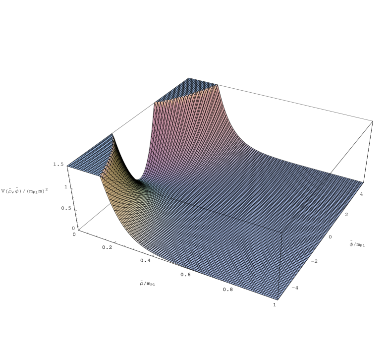
Figure 1: Potential $V(\bar{\rho},\bar{\phi})$ given by Eq. (37) represented in terms of the normalized field $\bar{\phi}$ and $\bar{\rho}$. The potential possesses a minimum in the $\bar{\phi}$ direction but, as is obvious from the figure, not in the $\bar{\rho}$ direction. Hence, the moduli is not stabilized in this model.

IV Mutated chaotic inflation

IV.1 Giving a mass to the inflaton

In this section, we discuss a successful model of inflation combining moduli stabilization and chaotic inflation. To motivate the introduction of a mass term for the inflaton field, let us consider the D3/D7 system in string theory D3 ; Hsu ; koyama . This system can be modeled at low energy using three fields, the inflaton $\phi$ measuring the inter–brane distance and two charged fields $\phi^{\pm}$ representing the open strings between the two types of branes. The fields interact according to the superpotential

$$W\left(\phi,\phi^{+},\phi^{-}\right)=\sqrt{2}g\left(\phi^{+}\phi\phi^{-}-\zeta^{2}\phi\right)\,,$$ (38)

where $g$ is the $U(1)$ gauge coupling and $\zeta$ is a constant term which is turned on when the compactification looks like a resolution of an orbifold singularity $\mathbb{C}^{2}/\mathbb{Z}_{2}$ locally. The term $\zeta^{2}$ is stabilized at the same time as the complex structure moduli. This is not the case of the Fayet–Iliopoulos term which depends on the Kähler moduli. To simplify we consider the case where there is no Fayet-Iliopoulos term.

Let us also give the Kähler function of the model. As before, for the inflaton field $\phi$, we focus on the case where the function ${\cal K}$ vanishes and where ${\cal G}=-1/2\left(\phi-\phi^{\dagger}\right)^{2}$. On the other hand, the Kähler functions for the charged fields are standard and, therefore, the total Kähler function is given by

$$K\left(\phi,\phi^{+},\phi^{-}\right)=-\frac{1}{2}\left(\phi-\phi^{\dagger}\right)^{2}+\phi^{+}\left(\phi^{+}\right)^{\dagger}+\phi^{-}\left(\phi^{-}\right)^{\dagger}\,.$$ (39)

As we discussed in the introduction, stabilizing moduli can be achieved by considering non-perturbative superpotentials springing from gaugino condensation. In this case, the superpotential contains a part which explicitly depends on the moduli and reads

$$W(\rho)=W_{0}-A\exp\left(-\beta\kappa^{1/2}\rho\right)\,,$$ (40)

where $W_{0}$, $A$ are free constants of dimension three and $\beta$ is dimensionless. The superpotential $W(\rho)$ has already been studied in Refs. KKLT and Tye . In string theory, the constant term springs from the stabilization of both the complex structure moduli and the dilaton. The exponential term is of non-perturbative origin. We take the total superpotential of the system to be the sum of the two previous expression, namely

$$W\left(\phi,\phi^{+},\phi^{-},\rho\right)=W\left(\phi,\phi^{+},\phi^{-}\right)+W(\rho)\,.$$ (41)

It is known from string considerations that the coupling constant $g$ and/or $\zeta$ can not depend on the moduli $\rho$ D3 . Therefore, this superpotential is the simplest way of coupling the moduli to inflation.

Finally, the total Kähler potential is also the sum of the Kähler potentials in the inflaton and moduli sector. It can be expressed as

$$K\left(\phi,\phi^{+},\phi^{-},\rho\right)=K\left(\phi,\phi^{+},\phi^{-}\right)-\frac{3}{\kappa}\ln\left[\kappa^{1/2}\left(\rho+\rho^{\dagger}\right)\right]\,.$$ (42)

Having specified what the Kähler and super potentials of the model are, one can now determine the corresponding scalar potential. It reads

$$V = \frac{{\rm e}^{\kappa\left(|\phi^{+}|^{2}+|\phi^{-}|^{2}\right)}}{\kappa^{3/2}\left(\rho+\rho^{\dagger}\right)^{3}}\biggl{\{}\left|\sqrt{2}g\phi\phi^{-}+\kappa\left(\phi^{+}\right)^{\dagger}W\right|^{2}+\left|\sqrt{2}g\phi\phi^{+}+\kappa\left(\phi^{-}\right)^{\dagger}W\right|^{2}+2g^{2}\left|\phi^{+}\phi^{-}-\zeta^{2}\right|^{2}$$ (43)

$$-2\kappa^{3/2}\beta A\left(\rho+\rho^{\dagger}\right)\Re\left[{\rm e}^{-\beta\kappa^{1/2}\rho^{\dagger}}W\left(\phi,\phi^{+},\phi^{-}\right)\right]\biggr{\}}+{\rm e}^{\kappa\left(|\phi^{+}|^{2}+|\phi^{-}|^{2}\right)}\tilde{\cal V}(\rho)+\frac{g^{2}}{2}\left(\left|\phi^{+}\right|^{2}-\left|\phi^{-}\right|^{2}\right)^{2}\,,$$

where $y\equiv\beta\kappa^{1/2}\rho$ and where $W$ in the previous formula denotes the total superpotential defined by Eq. (41). The function $\tilde{\cal V}(\rho)$ is defined by

$$\tilde{\cal V}(\rho)\equiv\frac{\kappa A\beta^{2}}{2y}{\rm e}^{-y}\left[\frac{A\beta}{3}{\rm e}^{-y}-\frac{\beta}{y}\left(W_{0}-A{\rm e}^{-y}\right)\right]\,.$$ (44)

The true vacuum of the above potential is obtained for $\phi^{+}=\phi^{-}=\zeta$, $\phi=-\kappa W(\rho_{{\rm min},\tilde{\cal V}})/(\sqrt{2}g)$, $\rho=\rho_{{\rm min},\tilde{\cal V}}$ being the minimum of the function $\tilde{\cal V}$. This leads to an AdS vacuum with unbroken supersymmetry KKLT .

For large $\phi$ compared to $\zeta$, the potential has a flat inflationary valley where $\phi^{\pm}=0$ and the slope of the potential can be lifted by radiative corrections. When $\phi$ becomes small compared to $\zeta$, the field $\phi^{\pm}$ run towards the true minimum $\phi^{+}=\phi^{-}=\zeta$ and $\phi=-\kappa W/(\sqrt{2}g)$. This realizes a hybrid inflation scenario in string theory.

Now, let us consider the situation where $\phi$ is small enough and the charged fields are stuck at the minimum. In this regime, the field $\phi$ can be expanded according to

$$\phi\simeq-\frac{\kappa W\left(\rho\right)}{\sqrt{2}g}+\delta\chi\,.$$ (45)

Then the field $\delta\chi$ becomes massive with a potential

$$V=\tilde{\cal V}(\rho)+\frac{4g^{2}\zeta^{2}}{\kappa^{3/2}(\rho+\rho^{\dagger})^{3}}\left|\delta\chi\right|^{2}\,.$$ (46)

We now notice that this potential can be also obtained using the much simpler superpotential

$$W(\rho,\phi)=W(\rho)+g\zeta(\delta\chi)^{2}\,,$$ (47)

in the global supersymmetry limit where the Planck mass is taken to be very large compared to the inflation scale. This provides a motivation to use the above superpotential in a regime where supergravity corrections are taken into account and where one can be far from the true minimum. We show in the next subsection that the potential becomes very interesting and leads to “mutated chaotic inflation”.

IV.2 The model

Following the considerations presented before, we assume that the inflaton is a massive field like in chaotic inflation and discuss its coupling to the moduli stabilization sector. Since our model is a string inspired, we take ${\cal K}=0$ and ${\cal G}=-1/2\left(\phi-\phi^{\dagger}\right)^{2}$ for the Kähler potential. For the superpotential, we use the calculation of the previous subsection section and assume that

$$W(\rho,\phi) = W(\rho)+W_{\rm inf}(\phi)$$ (48)

$$= W_{0}-A\exp\left(-\beta\kappa^{1/2}\rho\right)+\frac{\alpha}{2}m\phi^{2}\,,$$

where the mass $m$ can be related to $\zeta$, namely $m=2g\zeta/\alpha$. Then, we use the general formula established before, see Eqs. (24) and (25), and we obtain

$$V\left(\rho,\phi\right)=\tilde{{\cal V}}(\rho)+\tilde{{\cal U}}(\rho)\phi^{2}\,,$$ (49)

where the function $\tilde{\cal V}$ has already been defined above in Eq. (44) and $\tilde{\cal U}$ given by

$$\tilde{{\cal U}}(\rho)=\frac{\alpha m\beta^{3}}{4y^{2}}\left(\frac{\alpha m}{2y}-\kappa A{\rm e}^{-y}\right)\,,$$ (50)

and where we remind that $y\equiv\beta\kappa^{1/2}\rho$. Let us notice that, if $\kappa\rightarrow 0$, then $\tilde{\cal U}\sim 1/\rho^{3}$ in accordance with Eq. (46). The function $\tilde{\cal U}(\rho)$, from the point of view of the field $\phi$, plays the role of an effective squared mass. The function $\tilde{\cal V}(\rho)$ is not multiplied by a function of the field $\phi$ and, therefore, can be viewed as an “offset”. In order for the above potential to be relevant, it is necessary for the effective squared mass to be positive at the extremum of $\tilde{\cal U}$ where the moduli is stabilized.

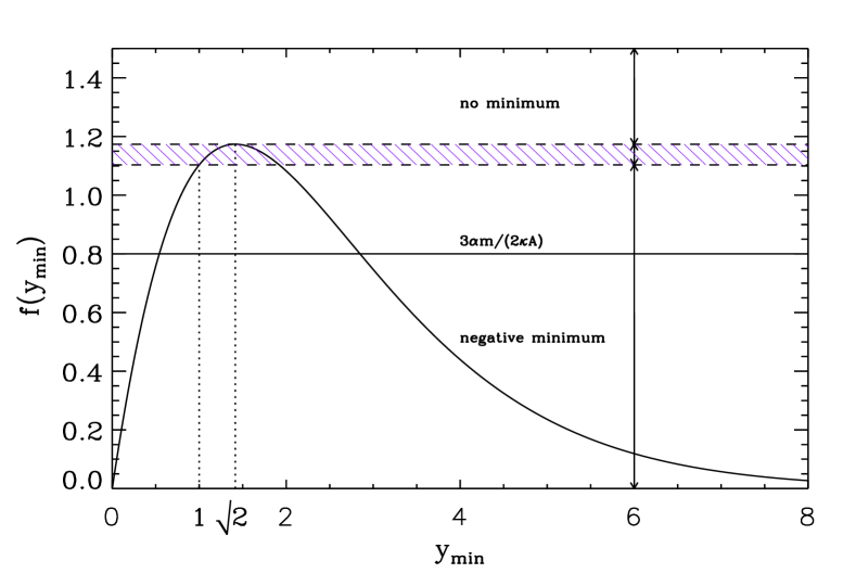
Figure 2: The function $f\left(y_{{\rm min},\tilde{\cal U}}\right)$ defined in Eq. (54). The maximum of this function is located at $y_{{\rm min},\tilde{\cal U}}=\sqrt{2}$ and is equal to $1.17387$. The intersection of $f\left(y_{{\rm min},\tilde{\cal U}}\right)$ with the horizontal line (solid line) $3\alpha m/(2\kappa A)$ determines the value(s) of $\rho$ corresponding to the extrema of the function $\tilde{\cal U}$. According to the values of the parameter $m$ and $A$, the line moves up or downwards while the function $f\left(y_{{\rm min},\tilde{\cal U}}\right)$ remains the same. As explained in the text, if the line is above the maximum of $f(y_{{\rm min},\tilde{\cal U}})$ then there are no extrema. If the line is below the maximum, there are always two extrema. The first intersection between $f\left(y_{{\rm min},\tilde{\cal U}}\right)$ and the horizontal line [in the increasing part of the function $f\left(y_{{\rm min},\tilde{\cal U}}\right)$] corresponds to a minimum while the second intersection corresponds to a maximum. However, if the line is below the value $3/{\rm e}\simeq 1.10364$, the corresponding value of $\tilde{\cal U}$ is negative. The effective squared mass $\tilde{\cal U}$ is positive at the minimum if the horizontal line is in the dashed area which, therefore, represents the allowed region.

Let us also give the potential in terms of the normalized fields $\bar{\rho}$ and $\bar{\phi}$. These fields are given by the formulas in the text before Eq. (37) since the Kähler potential in the present section is the same as in the subsection of Eq. (37). Below, for convenience, we reproduce the relation between canonical and non-canonical fields

$$\phi=\frac{\bar{\phi}}{\sqrt{2}}\,,\quad y=\beta\exp\left(\sqrt{\frac{2}{3}}\kappa^{1/2}\bar{\rho}\right)\,.$$ (51)

Therefore, the potential reads

$$V\left(\bar{\rho},\bar{\phi}\right) = \frac{\kappa A\beta}{2}{\rm e}^{-\sqrt{2/3}\kappa^{1/2}\bar{\rho}}\exp\left(-\beta{\rm e}^{\sqrt{2/3}\kappa^{1/2}\bar{\rho}}\right)\biggl{\{}\frac{A\beta}{3}\exp\left(-\beta{\rm e}^{\sqrt{2/3}\kappa^{1/2}\bar{\rho}}\right)$$ (52)

$$-{\rm e}^{-\sqrt{2/3}\kappa^{1/2}\bar{\rho}}\left[W_{0}-A\exp\left(-\beta{\rm e}^{\sqrt{2/3}\kappa^{1/2}\bar{\rho}}\right)\right]\biggr{\}}$$

$$+\frac{\alpha m\beta}{8}{\rm e}^{-2\sqrt{2/3}\kappa^{1/2}\bar{\rho}}\left[\frac{\alpha m}{2\beta}{\rm e}^{-\sqrt{2/3}\kappa^{1/2}\bar{\rho}}-\kappa A\exp\left(-\beta{\rm e}^{\sqrt{2/3}\kappa^{1/2}\bar{\rho}}\right)\right]\bar{\phi}^{2}\,.$$

Notice that, since the link between $(\rho,\phi)$, on one hand, and $(\bar{\rho},\bar{\phi})$, on the other hand, is monotonic, the above change of variables does not modify the properties of the minima. In particular, in order to study how these properties depend on the free parameters, it is sufficient to work in terms of the non-canonically normalized fields which is simpler.

IV.3 The squared mass function $\tilde{\cal U}(\rho)$

We now analyze whether the moduli can be stabilized to a value corresponding to a positive potential. For this purpose, we study the effective squared mass function $\tilde{\cal U}$ and requires that this function has a positive minimum. We will see that the valley where the moduli is stabilized is not exactly given by the minimum of the function $\tilde{\cal U}$ because, for small values of $\phi$, the offset function $\tilde{\cal V}$ also plays a role. In fact, strictly speaking, the minimum of $\tilde{\cal U}$ is the valley of stability for $\phi/m_{{}_{\mathrm{P}l}}\rightarrow+\infty$ only. However, we emphasize that it is mandatory that the true minimum of $\tilde{\cal U}$ be positive since this term is multiplied by $\phi^{2}$. Otherwise the inflaton field becomes tachyonic. It is easy to calculate the derivative of the effective mass $\tilde{\cal U}$. This gives

$$\frac{{\rm d}\tilde{\cal U}}{{\rm d}y}=\frac{\alpha m\beta^{3}}{4y^{4}}\left(-\frac{3}{2}\alpha m+2\kappa Ay{\rm e}^{-y}+\kappa Ay^{2}{\rm e}^{-y}\right)\,.$$ (53)

It vanishes at $y=y_{{\rm min},\tilde{\cal U}}$ where $y_{{\rm min},\tilde{\cal U}}$ satisfies the following equation

$$f\left(y_{{\rm min},\tilde{\cal U}}\right)=y_{{\rm min},\tilde{\cal U}}\left(y_{{\rm min},\tilde{\cal U}}+2\right){\rm e}^{-y_{{\rm min},\tilde{\cal U}}}=\frac{3\alpha m}{2\kappa A}\,.$$ (54)

From this expression, one gets a constraint on the parameters $m$ and $A$, coming from the fact that $3\alpha m/(2\kappa A)$ must be smaller than the maximum value of the function $y_{{\rm min},\tilde{\cal U}}(y_{{\rm min},\tilde{\cal U}}+2){\rm e}^{-y_{{\rm min},\tilde{\cal U}}}$, otherwise the above equation has no solution, see Fig. 2. This function vanishes at the origin, increases and reaches a maximum at $y_{{\rm min},\tilde{\cal U}}=\sqrt{2}$ and then exponentially decreases towards zero. Therefore, the function $\tilde{\cal U}$ possesses an extremum if and only if $0<3\alpha m/(2\kappa A)<\sqrt{2}\left(2+\sqrt{2}\right){\rm e}^{-\sqrt{2}}\simeq 1.17387$. The value of $\tilde{\cal U}$ at the extremum can be easily derived and one obtains

$$\tilde{\cal U}\left(y=y_{{\rm min},\tilde{\cal U}}\right)=\frac{\alpha^{2}m^{2}\beta^{3}}{8y_{{\rm min},\tilde{\cal U}}^{3}}\frac{y_{{\rm min},\tilde{\cal U}}-1}{y_{{\rm min},\tilde{\cal U}}+2}\,.$$ (55)

Therefore, the extremum corresponds to a positive potential if $y_{{\rm min},\tilde{\cal U}}>1$ but, at this level, this does not require new constraints on $m$ and $A$.

Figure 3: Left panel: function $\tilde{\cal U}(\rho)$ for three different values of the ratio $\kappa A/(\alpha m)$. The dashed line corresponds to a situation where there is no minimum, i.e. the line $3\alpha m/(2\kappa A)$ is above the function $f\left(y_{{\rm min},\tilde{\cal U}}\right)$, see Fig. 2. The dotted line represents the case where there is a positive minimum, i.e. the line $3\alpha m/(2\kappa A)$ is within the dashed area in Fig. 2. Finally, the solid line corresponds to a function $\tilde{\cal U}$ with a negative minimum. Right panel: function $\tilde{\cal V}(\rho)$ for three different values of the ratio $W_{0}/A$. One can check on the figure that, if $W_{0}/A<1$ then there is a negative minimum and $\lim_{y\rightarrow 0}\tilde{\cal V}=+\infty$ while, if $W_{0}/A>1$ there is no minimum but $\lim_{y\rightarrow 0}\tilde{\cal V}=-\infty$.

Now, let us check whether this is a maximum or a minimum. For this purpose, one calculate the second derivative of $\tilde{\cal U}$ at the extremum. One obtains

$$\frac{{\rm d}^{2}\tilde{\cal U}}{{\rm d}y^{2}}\biggl{|}_{y=y_{{\rm min},\tilde{\cal U}}}=-\frac{3\alpha^{2}m^{2}\beta^{3}}{8}\frac{y_{{\rm min},\tilde{\cal U}}^{2}-2}{y_{{\rm min},\tilde{\cal U}}^{5}\left(y_{{\rm min},\tilde{\cal U}}+2\right)}\,.$$ (56)

This is positive if $y_{{\rm min},\tilde{\cal U}}<\sqrt{2}$. Therefore, we have a positive minimum if the parameters $m$ and $A$ are such that $1<y_{{\rm min},\tilde{\cal U}}<\sqrt{2}$ which in turn implies that one must have $3/{\rm e}\simeq 1.10364<3\alpha m/(2\kappa A)<\sqrt{2}\left(2+\sqrt{2}\right){\rm e}^{-\sqrt{2}}\simeq 1.17387$ or

$$1.27782<\frac{\kappa A}{\alpha m}<1.35914\,.$$ (57)

This interval is represented in Fig. 2 by the dashed region. It is quite clear from the above considerations that the ratio $m/(\kappa A)$ has to be adjusted precisely. However, this does not mean $m$ and/or $\kappa A$ must be tuned very accurately. As a matter of fact, they can a priori change over a large range of values, provided of course that their ratio satisfies the constraint derived above. The function $\tilde{\cal U}$ for various values of $m/(\kappa A)$ is represented in Fig. 3.

IV.4 The offset function $\tilde{\cal V}(\rho)$

Let us now study the effective offset function $\tilde{\cal V}(\rho)$ in more details. Firstly, let us evaluate

$$\frac{{\rm d}\tilde{\cal V}}{{\rm d}y}=-\frac{\kappa A^{2}\beta^{3}}{3y^{3}}{\rm e}^{-2y}\left[y^{2}+\frac{7}{2}y+3-\frac{3W_{0}}{2A}{\rm e}^{y}(y+2)\right]\,,$$ (58)

and, therefore, there is a minimum if the following equation is satisfied

$$y_{{\rm min},\tilde{\cal V}}^{2}+\frac{7}{2}y_{{\rm min},\tilde{\cal V}}+3=\frac{3W_{0}}{2A}{\rm e}^{y_{{\rm min},\tilde{\cal V}}}\left(y_{{\rm min},\tilde{\cal V}}+2\right)\,.$$ (59)

The existence of a solution to the above equation is controlled by the ratio $W_{0}/A$. If $W_{0}/A>1$, then there is no solution because the parabola in Eq. (59) cannot intersect the function $3W_{0}/(2A){\rm e}^{y_{{\rm min},\tilde{\cal V}}}\left(y_{{\rm min},\tilde{\cal V}}+2\right)$ (notice that for $W_{0}/A=1$ the two functions are equal at $y_{{\rm min},\tilde{\cal V}}=0$). Moreover, in this situation, we have $\lim_{y\rightarrow 0}\tilde{\cal V}=-\infty$ and, therefore, the function $\tilde{\cal V}$ cannot be positive everywhere. On the other hand, if $W_{0}/A<1$, then $\lim_{y\rightarrow 0}\tilde{\cal V}=+\infty$ and, in addition, Eq. (59) admits a solution, hence $\tilde{\cal V}$ possesses an extremum. Since we also have

$$\frac{{\rm d}^{2}\tilde{\cal V}}{{\rm d}y^{2}}\biggl{|}_{y=y_{{\rm min},\tilde{\cal V}}}=\frac{3\kappa W_{0}^{2}\beta^{3}\left(y_{{\rm min},\tilde{\cal V}}+2\right)}{8y_{{\rm min},\tilde{\cal V}}^{3}\left(y_{{\rm min},\tilde{\cal V}}^{2}+7y_{{\rm min},\tilde{\cal V}}/2+3\right)^{2}}$$ (60)

$$\times \left(2y_{{\rm min},\tilde{\cal V}}^{3}+9y_{{\rm min},\tilde{\cal V}}^{2}+12y_{{\rm min},\tilde{\cal V}}+4\right)>0\,,$$

the function $\tilde{\cal V}$ possesses an extremum which is a minimum. However, the value of this function at this minimum is given by

$$\tilde{\cal V}\left(y=y_{{\rm min},\tilde{\cal V}}\right)=-\frac{\kappa AW_{0}\beta^{3}}{4y_{{\rm min},\tilde{\cal V}}}$$ (61)

$$\times \frac{y_{{\rm min},\tilde{\cal V}}+2}{y_{{\rm min},\tilde{\cal V}}^{2}+7y_{{\rm min},\tilde{\cal V}}/2+3}{\rm e}^{-y_{{\rm min},\tilde{\cal V}}}<0\,.$$

As a consequence, the function $\tilde{\cal V}$ cannot be positive everywhere since it is negative at its extremum. However, this is not automatically a problem, as it would have been for the function $\tilde{\cal U}$, since the offset function can always be “renormalized” by adding a positive cosmological constant, namely $-\tilde{\cal V}\left(y=y_{{\rm min},\tilde{\cal V}}\right)$. We conclude from the above analysis that the function $\tilde{\cal V}$, regardless of the values of the free parameters $A$ and $W_{0}$, is necessarily negative somewhere. The regime of interest is given by $W_{0}/A<1$ since in this case $\tilde{\cal V}$ possesses a minimum which can be “renormalized” by adding a constant. The function $\tilde{\cal V}(\rho)$ is represented in Fig. 3 for various values of the ratio $W_{0}/A$.

Another remark is in order in this subsection. In the following, we will study another mechanism of stabilization (i.e. the KKLT mechanism) which consists in adding a term $\propto 1/\rho^{3}$ to the offset function. In this case one will show that one can always find a positive minimum regardless of $W_{0}/A$. Therefore, with this other mechanism, the above discussion of the shape of the offset function is modified and the condition $W_{0}/A<1$ can be relaxed.

Let us now discuss another class of models. In our models, inflation is only driven by the $F$ –terms originating from non–shift symmetric superpotentials. This is enough to lift the inflaton flat direction and leads to an inflation potential with no ${\cal O}(H)$ corrections to the inflaton mass. Of course we need to introduce a superpotential of chaotic inflation with a fine–tuning of the inflaton mass scale (see below where we apply the COBE normalization). This is the usual flatness problem in inflation model building. It has been argued in Ref. mac that such a fine–tuning is also present in string compactification where threshold corrections are taken into account leading to a superpotential of the form

$$W(\rho,\phi)=W(\rho)\left(1+\delta\kappa\phi^{2}\right)\,,$$ (62)

where $\delta$ has to be small to guarantee a small enough mass of the inflaton. This requires a tuning of the complex structure moduli. For this model the scalar potential becomes

$$V\left(\rho,\phi\right)=\tilde{\cal V}(\rho)\left(1+\delta\kappa\phi^{2}\right)^{2}+\frac{4\kappa^{2}\delta^{2}}{3\Delta^{2}}\left|W(\rho)\right|^{2}\phi^{2}\,,$$ (63)

where the Kähler potential corresponds to ${\cal G}=0$ and ${\cal K}=-(\phi-\phi^{\dagger})^{2}/2$ and where $\tilde{\cal V}$ is the same function as studied above. For large $\phi$ the potential reduces to

$$V\left(\rho,\phi\right)\simeq\tilde{\cal V}(\rho)\delta^{2}\kappa^{4}\phi^{4}\,.$$ (64)

Now, when $\rho$ is at the minimum of ${\tilde{\cal V}}$, the coupling constant of the $\phi^{4}$ term becomes negative implying that this potential is not suitable to obtain inflation. This exemplifies how difficult it is to find a satisfactory model of inflation in supergravity.

IV.5 Renormalizing the offset function by a constant

Having studied the functions $\tilde{\cal V}$ and $\tilde{\cal U}$ in some details, let us now turn to the properties of the full potential when shifted by a positive cosmological constant. It is represented in Fig. 4.

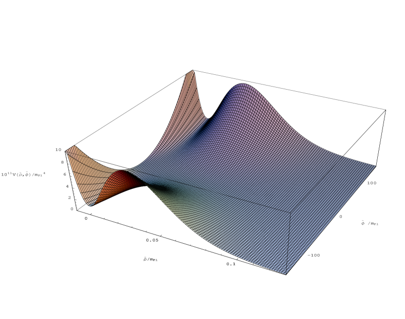
Figure 4: Potential $V(\bar{\rho},\bar{\phi})$ [what is actually plotted is $10^{11}V(\bar{\rho},\bar{\phi})/m_{{}_{\mathrm{P}l}}^{4}$] for the following choice of parameters: $\alpha=\sqrt{2}$, $\beta=1$, $m=10^{-6}m_{{}_{\mathrm{P}l}}$, $\kappa A/(\alpha m)=1.35135$ and $W_{0}/A=0.41111$. This gives an absolute minimum of the potential located at $\bar{\phi}=0$, $\bar{\rho}_{\rm min,\tilde{\cal V}}\simeq 0.1181\times m_{{}_{\mathrm{P}l}}$. These parameters satisfy the constraints derived in the text. The moduli is stabilized at the value $y=y_{\rm min,\tilde{\cal U}}\simeq 1.016$ or $\bar{\rho}_{\rm min,\tilde{\cal U}}\simeq 0.0040\times m_{{}_{\mathrm{P}l}}$ (for $\bar{\phi}\gg m_{{}_{\mathrm{P}l}}$) as can be checked in the figure where the inflationary valley is clearly seen.

The derivatives of the potential in the two directions $\bar{\rho}$ and $\bar{\phi}$ are given by

$$\frac{\partial V}{\partial\bar{\phi}} = \frac{{\rm d}\phi}{{\rm d}\bar{\phi}}\frac{\partial V}{\partial\phi}=\frac{1}{\sqrt{2}}\times 2\tilde{\cal U}\phi\,,$$ (65)

$$\frac{\partial V}{\partial\bar{\rho}} = \frac{{\rm d}y}{{\rm d}\bar{\rho}}\frac{\partial V}{\partial y}=\sqrt{\frac{2}{3}}\kappa^{1/2}y\left(\frac{{\rm d}\tilde{\cal V}}{{\rm d}y}+\frac{{\rm d}\tilde{\cal U}}{{\rm d}y}\phi^{2}\right)\,.$$ (66)

From these expressions, we deduce that the potential possesses an absolute minimum located at

$$\bar{\phi}=0\,,\quad\bar{\rho}={\bar{\rho}}_{\rm min,\tilde{\cal V}}\,.$$ (67)

At this minimum, the potential vanishes exactly.

From the expressions of the derivatives of the potential, Eqs. (65) and (66), one deduces that there also exists a valley of stability. This valley is also clearly seen in Fig. 4 and is of course of utmost importance for us. It is given by the following trajectory in the $(\rho,\phi)$ plane

$$\kappa\phi^{2}_{\rm valley}\left(y\right)=\frac{4}{3}\left(\frac{\kappa A}{\alpha m}\right)^{2}y{\rm e}^{-2y}\left[y^{2}+\frac{7}{2}y+3-\frac{3}{2}\frac{W_{0}}{A}{\rm e}^{y}\left(y+2\right)\right]\times\left[-\frac{3}{2}+2\left(\frac{\kappa A}{\alpha m}\right)y{\rm e}^{-y}+\left(\frac{\kappa A}{\alpha m}\right)y^{2}{\rm e}^{-y}\right]^{-1}\,.$$ (68)

In terms of canonically normalized fields, the same trajectory reads

$$\kappa\bar{\phi}^{2}_{\rm valley}\left(\bar{\rho}\right) = \frac{8}{3}\left(\frac{\kappa A}{\alpha m}\right)^{2}\beta{\rm e}^{\sqrt{\frac{2}{3}}\kappa^{1/2}\bar{\rho}}\exp\left(-2\beta{\rm e}^{\sqrt{\frac{2}{3}}\kappa^{1/2}\bar{\rho}}\right)\biggl{[}\beta^{2}{\rm e}^{2\sqrt{\frac{2}{3}}\kappa^{1/2}\bar{\rho}}+\frac{7}{2}\beta{\rm e}^{\sqrt{\frac{2}{3}}\kappa^{1/2}\bar{\rho}}+3$$ (69)

$$-\frac{3}{2}\frac{W_{0}}{A}\exp\left(\beta{\rm e}^{\sqrt{\frac{2}{3}}\kappa^{1/2}\bar{\rho}}\right)\left(\beta{\rm e}^{\sqrt{\frac{2}{3}}\kappa^{1/2}\bar{\rho}}+2\right)\biggr{]}\times\biggl{[}-\frac{3}{2}+2\left(\frac{\kappa A}{\alpha m}\right)\beta{\rm e}^{\sqrt{\frac{2}{3}}\kappa^{1/2}\bar{\rho}}\exp\left(-\beta{\rm e}^{\sqrt{\frac{2}{3}}\kappa^{1/2}\bar{\rho}}\right)$$

$$+\left(\frac{\kappa A}{\alpha m}\right)\beta^{2}{\rm e}^{2\sqrt{\frac{2}{3}}\kappa^{1/2}\bar{\rho}}\exp\left(-\beta{\rm e}^{\sqrt{\frac{2}{3}}\kappa^{1/2}\bar{\rho}}\right)\biggr{]}^{-1}\,.$$

This trajectory is represented in Fig. 5.

Figure 5: Trajectory of the valley of stability in the plan $(\bar{\rho},\bar{\phi})$ (the valley is seen from above). For large values of $\bar{\phi}$, $\bar{\phi}\gg m_{{}_{\mathrm{P}l}}$, the valley coincides with the minimum of the function $\tilde{\cal U}$, i.e. is just given by the equation $\bar{\rho}=\bar{\rho}_{\rm min,\tilde{\cal U}}$. For smaller values of the inflaton, the trajectory bends and quickly joins the absolute minimum of the potential, namely $y=y_{\rm min,\tilde{\cal V}}$, $\phi=0$. The parameters used here are: $\alpha=\sqrt{2}$, $\beta=1$, $m=10^{-6}m_{{}_{\mathrm{P}l}}$, $\kappa A/(\alpha m)=1.35135$ and $W_{0}/A=0.41111$. This gives $y=y_{\rm min,\tilde{\cal U}}\simeq 1.016$ or $\bar{\rho}_{\rm min,\tilde{\cal U}}\simeq 0.0040\times m_{{}_{\mathrm{P}l}}$ and the global minimum of the potential is located at $\bar{\phi}=0$, $\bar{\rho}_{\rm min,\tilde{\cal V}}\simeq 0.1181\times m_{{}_{\mathrm{P}l}}$.

For large values of the inflaton, $\bar{\phi}/m_{{}_{\mathrm{P}l}}\gg 1$, the offset function is negligible and the potential is almost given by $V\simeq\tilde{\cal U}\phi^{2}$. As a consequence, the valley of stability reduces to the simple equation $\bar{\rho}=\bar{\rho}_{\rm min,\tilde{\cal U}}$ as can be directly checked in Fig. 5: in this regime (but in this regime only), as it is the case for hybrid inflation, the waterfall field is frozen. For small values of $\bar{\phi}/m_{{}_{\mathrm{P}l}}$, the offset function becomes important, the trajectory bends and, as expected, joins the global minimum of the potential .

Let us now discuss how inflation proceeds in this model. Clearly, the potential plotted in Fig. 4 is reminiscent of hybrid inflation where $\bar{\phi}$ is the inflaton and where the moduli $\bar{\rho}$ plays the role of the waterfall field hybrid . In hybrid inflation, inflation proceeds along the valley either in the vacuum dominated regime, in which case the potential is almost a constant, or in the inflaton dominated regime, in which case $V\sim\phi^{2}$. There is also a version, well-motivated from the particle physics point of view, where the flat valley is lifted by quantum corrections LR . In this case the potential along the valley is computed by means of the well-known Coleman-Weinberg formula. In our case, we have already noticed that, for $\bar{\phi}\gg m_{{}_{\mathrm{P}l}}$, the potential in the valley takes the form $V\sim\tilde{\cal U}\bar{\phi}^{2}$. Therefore, our case belongs to the inflaton dominated regime case.

The next question is to study how inflation ends. Typically, in hybrid inflation, inflation stops by instability. At some point along the inflationary valley, the effective squared mass in the direction perpendicular to the valley becomes negative and, as a consequence, the field can no longer be kept on tracks and quickly rolls down towards its minimum where reheating proceeds. We will show that this is not the case here. In our case, inflation stops while still in the valley due to a violation of the slow-roll conditions. The crucial ingredient here is that the valley is not a straight line but corresponds to a non-trivial path in the configuration space of the two fields. This aspect is reminiscent of mutated inflation mutated (other interesting inflationary models where the trajectory is not trivial can be found in Refs. shifted ). In fact, the analogy can even been pushed further. Indeed, in the case of mutated inflation, the potential has typically the following form LR

$$V\left(\psi,\phi\right)=V_{0}\left(1-\frac{\psi}{M}\right)+\frac{\lambda}{4}\phi^{2}\psi^{2}+\cdots\,,$$ (70)

where $V_{0}$, $M$ and $\lambda$ are constants. In the above expression, $\phi$ is the inflaton and the second field $\psi$ plays the role of our moduli $\rho$. One of the main feature of mutated inflation is that an effective potential for the inflaton can be produced even if the original potential contains no term that depends only on $\phi$ as can be seen explicitly in the previous formula. In the configuration space, the trajectory reads $\psi\phi^{2}=2V_{0}/(\lambda M)$ and after having inserted this expression into Eq. (70) one gets

$$V\left(\phi\right)=V_{0}\left(1-\frac{V_{0}}{\lambda^{2}M^{2}\phi^{2}}\right)\,,$$ (71)

which is suitable for inflation. In the same manner, our potential given in Eq. (49) does not contain any piece depending on the inflaton field only. However, inserting the trajectory $\rho(\phi)$ in $V\left(\rho,\phi\right)$ would lead to a potential $V(\phi)$ as above. The difficulty in our case is that Eq. (68) gives rather $\phi(\rho)$ and that the expression is too complicated to be invertible. But, clearly, at the level of principles this is very similar. Therefore, the model presented here combines aspects from chaotic and mutated inflation hence the name “mutated chaotic inflation” given at the beginning of this section.

IV.6 Phenomenological constraints

We now discuss the constraint on the parameter characterizing the inflaton sector, i.e. the mass $m$ (since the parameters $A$ and $W_{0}$ have already been discussed before). In order to simplify the discussion, we will assume that the initial conditions are such that the fields are, at the beginning of the evolution, in the valley of stability and more particularly in the straight line part of the valley (we will come back to the questions of the initial conditions later on and will discuss this assumption in some detail) where $V\sim\tilde{\cal U}\left(\bar{\rho}_{\rm min,\tilde{\cal U}}\right)\bar{\phi}^{2}/2$. Since the quantum fluctuations of the inflaton field $\bar{\phi}$ are at the origin of the CMB anisotropy observed today, the COBE and Wilkinson Microwave Anisotropy Probe (WMAP) normalizations fix the coupling constant of the inflaton potential, namely the mass function $\tilde{\cal U}\left(\bar{\rho}_{\rm min,\tilde{\cal U}}\right)$ in the present context. Concretely, for small $\ell$, the multipole moments are given by

$$C_{\ell}=\frac{2H^{2}}{25\epsilon m_{{}_{\mathrm{P}l}}^{2}}\frac{1}{\ell(\ell+1)}\,,$$ (72)

where $\epsilon$ is the first slow-roll parameter to be discussed below. What has been actually measured by the COBE and WMAP satellites is $Q^{2}_{\rm rms-PS}/T^{2}=5C_{2}/(4\pi)\simeq\left(18\times 10^{-6}/2.7\right)^{2}\simeq 36\times 10^{-12}$. The quantity $H$ is the Hubble parameter during inflation and is related to the potential by the slow-roll equation $H^{2}\simeq\kappa V/3$ evaluated at Hubble radius crossing. Putting everything together, we find that the inflaton mass is given by

$$\left[\frac{\tilde{\cal U}\left(\bar{\rho}_{\rm min,\tilde{\cal U}}\right)}{m_{{}_{\mathrm{P}l}}}\right]^{2}\simeq 45\pi\left(N_{*}+\frac{1}{2}\right)^{-2}\frac{Q^{2}_{\rm rms-PS}}{T^{2}}\,,$$ (73)

where $N_{*}\simeq 60$ (i.e. the number of e-folds between the time at which the modes of astrophysical interest today left the Hubble radius during inflation and the end of inflation, see Ref. number ), that is to say

$$\sqrt{\tilde{\cal U}\left(\bar{\rho}_{\rm min,\tilde{\cal U}}\right)}\simeq 1.3\times 10^{-6}\times m_{{}_{\mathrm{P}l}}\,.$$ (74)

At this point, it is important to recall that the mass function has been defined by the expression

$$\tilde{\cal U}\left(\bar{\rho}_{\rm min,\tilde{\cal U}}\right)=\frac{(\alpha m)^{2}\beta^{3}}{4y_{\rm min,\tilde{\cal U}}}\left(\frac{1}{2y_{\rm min,\tilde{\cal U}}}-\frac{\kappa A}{\alpha m}{\rm e}^{-y_{\rm min,\tilde{\cal U}}}\right)\,.$$ (75)

In this expression, all the factors but $m$ are of order one, see the previous discussion about the constraints on the parameters $A$ and $W_{0}$. Therefore, this implies that $m\simeq{\cal O}\left(10^{-6}\right)$ and this is the value that will be used in the following.

In order to compute the inflationary observables (as the spectral indices for instance), it is convenient to use the slow-roll approximation. The slow-roll approximation is controlled by two parameters (in fact, at leading order, there are three relevant slow-roll parameters but we will not need the third one) defined by slowroll

$$\epsilon \equiv -\frac{\dot{H}}{H^{2}}\,,\quad\delta=-\frac{\dot{\epsilon}}{2H\epsilon}+\epsilon\,.$$ (76)

The main advantage of these definitions is that they involve the background Hubble parameter $H$ only. Therefore, in some sense, they are independent from the matter content, in particular they do not require the knowledge of the number of scalar fields present in the underlying inflationary model. If we now assume that only one scalar field is present, then it is easy to obtain that

$$\epsilon \simeq \epsilon_{\bar{\phi}}\equiv\frac{m_{{}_{\mathrm{P}l}}^{2}}{16\pi}\left(\frac{V_{,{\bar{\phi}}}}{V}\right)^{2}\,,$$ (77)

$$\delta \simeq \delta_{\bar{\phi}}\equiv-\frac{m_{{}_{\mathrm{P}l}}^{2}}{16\pi}\left(\frac{V_{,\bar{\phi}}}{V}\right)^{2}+\frac{m_{{}_{\mathrm{P}l}}^{2}}{8\pi}\frac{V_{,\bar{\phi}\bar{\phi}}}{V}\,.$$ (78)

Two remarks are in order. Firstly, the condition $\epsilon<1$ is equivalent to $\ddot{a}>0$. Therefore, in order to have inflation, strictly speaking $\epsilon$ needs not to be small with respect to one, it only needs to be less than one. Secondly, the parameter $\delta$ is not positive definite contrary to the first slow-roll parameter.

In the case where two fields are present, they are different ways of generalizing the definition of the slow-roll parameters isopert . A first method consists in following the trajectory in configuration space. The trajectory is given by $\bar{\phi}=\bar{\phi}(N)$ and $\bar{\rho}=\bar{\rho}(N)$, where $N$ is the total number of e-folds counted from the beginning of inflation (not to be confused with $N_{*}$). As a consequence the vector tangent to this trajectory, ${\bf e}_{\parallel}=(e_{\bar{\phi}},e_{\bar{\rho}})$, can be expressed as

$$e_{\bar{\phi}} = \frac{\displaystyle\frac{{\rm d}\bar{\phi}}{{\rm d}N}}{\sqrt{\displaystyle\left(\frac{{\rm d}\bar{\phi}}{{\rm d}N}\right)^{2}+\left(\frac{{\rm d}\bar{\rho}}{{\rm d}N}\right)^{2}}}=\cos\theta\,,$$ (79)

$$e_{\bar{\rho}} = \frac{\displaystyle\frac{{\rm d}\bar{\rho}}{{\rm d}N}}{\sqrt{\displaystyle\left(\frac{{\rm d}\bar{\phi}}{{\rm d}N}\right)^{2}+\left(\frac{{\rm d}\bar{\rho}}{{\rm d}N}\right)^{2}}}=\sin\theta\,.$$ (80)

We can then define “directional slow-roll parameters” by replacing the first and second derivatives in Eqs. (77) by directional derivatives of the potential, namely

$$\epsilon_{\parallel} = \frac{m_{{}_{\mathrm{P}l}}^{2}}{16\pi V^{2}}\left(\cos\theta V_{,{\bar{\phi}}}+\sin\theta V_{,{\bar{\rho}}}\right)^{2}\,,$$ (81)

$$\delta_{\parallel} = -\epsilon_{\parallel}+\frac{m_{{}_{\mathrm{P}l}}^{2}}{8\pi V}(\cos^{2}\theta V_{,\bar{\phi}\bar{\phi}}+2\cos\theta\sin\theta V_{,\bar{\phi}\bar{\rho}}$$ (82)

$$+\sin^{2}\theta V_{,\bar{\rho}\bar{\rho}})\,.$$

However, it is clear that we no longer have the equivalence between $\epsilon_{\parallel}<1$ and $\ddot{a}>0$. For this reason, it is also interesting to keep the original definition of $\epsilon$ (only in terms of the “geometry”), i.e. $\epsilon=-\dot{H}/H^{2}$, and express it in terms of the derivatives of the potential. This leads to

$$\epsilon=\epsilon_{\bar{\phi}}+\epsilon_{\bar{\rho}}=\frac{m_{{}_{\mathrm{P}l}}^{2}}{16\pi}\left(\frac{V_{,{\bar{\phi}}}}{V}\right)^{2}+\frac{m_{{}_{\mathrm{P}l}}^{2}}{16\pi}\left(\frac{V_{,{\bar{\rho}}}}{V}\right)^{2}\,.$$ (83)

It is interesting to establish the link between the two types of slow-roll parameters. For this purpose, let us introduce the vector ${\bf e}_{\perp}\equiv(e_{\bar{\rho}},-e_{\bar{\phi}})$, which is perpendicular to ${\bf e}_{\parallel}$. Then, one can define a directional slow-roll parameter in the direction perpendicular to the trajectory by means of the expression

$$\epsilon_{\perp}=\frac{m_{{}_{\mathrm{P}l}}^{2}}{16\pi V^{2}}\left(\sin\theta V_{,{\bar{\phi}}}-\cos\theta V_{,{\bar{\rho}}}\right)^{2}\,.$$ (84)

From this expression, it is not difficult to show that

$$\epsilon_{\parallel}+\epsilon_{\perp}=\epsilon_{\bar{\phi}}+\epsilon_{\bar{\rho}}=\epsilon\,.$$ (85)

Obviously, if the inflationary valley is a straight line then one has $\epsilon\simeq\epsilon_{\parallel}\simeq\epsilon_{\bar{\phi}}$ and this is the case for the model under consideration in this article provided that $\bar{\phi}\gg m_{{}_{\mathrm{P}l}}$. In this situation, the model is equivalent to chaotic inflation and therefore the slow-roll parameters are given by

$$\epsilon=\frac{1}{2N_{*}+1},\quad\delta=0\,,$$ (86)

where $N_{*}\simeq 60$ (there is some freedom in the choice of this number, see Ref. number ) has already been defined before. In the situation where these parameters are small, namely $\epsilon\ll 1$ and $\delta\ll 1$, the equation of motion of the inflaton field can be easily integrated. One finds

$$\frac{\bar{\phi}}{m_{{}_{\mathrm{P}l}}}=\sqrt{\left(\frac{\bar{\phi}_{\rm ini}}{m_{{}_{\mathrm{P}l}}}\right)^{2}-\frac{N}{2\pi}}\,,$$ (87)

where $\bar{\phi}_{\rm ini}$ is the initial value of the field. Let us emphasize again that this is valid only if the scales of astrophysical interest leave the Hubble radius in the straight line part of the potential. If this happens in the curved part of the potential the above result is no longer valid.

Finally, let us introduce the squared mass in the direction perpendicular to the inflationary trajectory. This is nothing but the second order directional derivative of the potential along ${\bf e}_{\perp}$ given by

$$m_{\perp}^{2}\equiv(\cos^{2}\theta V_{,\bar{\phi}\bar{\phi}}-2\cos\theta\sin\theta V_{,\bar{\phi}\bar{\rho}}+\sin^{2}\theta V_{,\bar{\rho}\bar{\rho}})\,.$$ (88)

This quantity allows us to distinguish whether inflation ends by instability or not. If, as it is the case for hybrid inflation, an instability occurs, $m_{\perp}^{2}$ becomes negative.

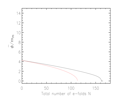
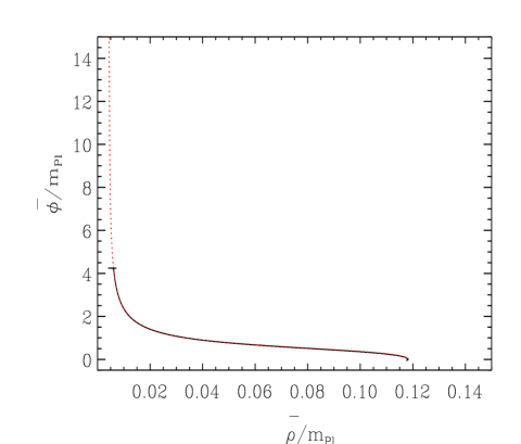
Figure 6: Evolution of the fields $\bar{\phi}$ and $\bar{\rho}$ together with the slow-roll parameters and the effective squared mass in the direction perpendicular to the inflationary trajectory. The parameters are $\alpha=\sqrt{2}$, $\beta=1$, $m=10^{-6}m_{{}_{\mathrm{P}l}}$, $\kappa A/(\alpha m)=1.35135$ and $W_{0}/A=0.41111$. This gives $y_{{\rm min},\tilde{\cal U}}\simeq 1.067$ or $\bar{\rho}_{{\rm min},\tilde{\cal U}}\simeq 0.004\times m_{{}_{\mathrm{P}l}}$. The absolute minimum of the potential is located at $\phi=0$, $y=y_{{\rm min},\tilde{\cal V}}\simeq 1.622$ or $\bar{\phi}=0$, $\bar{\rho}=\bar{\rho}_{{\rm min},\tilde{\cal V}}\simeq 0.118\times m_{{}_{\mathrm{P}l}}$. The initial conditions are $\phi_{\rm ini}=3\times m_{{}_{\mathrm{P}l}}$ or $\bar{\phi}_{\rm ini}\simeq 4.243\times m_{{}_{\mathrm{P}l}}$ and $y_{\rm ini}=y_{{\rm min},\tilde{\cal U}}\simeq 1.067$ or $\bar{\rho}_{\rm ini}=\bar{\rho}_{{\rm min},\tilde{\cal U}}\simeq 0.004\times m_{{}_{\mathrm{P}l}}$, i.e. at the bottom of the valley exactly. The interpretation of these plots is discussed in the text.

IV.7 Numerical results

To prove the above claims that inflation ends by violation of the slow-roll conditions and not by instability, it is necessary to determine the inflationary trajectory exactly. Clearly, the potential is too complicated to permit an analytical integration of the exact motion and, therefore, we will perform a numerical integration of the two Klein-Gordon equations and of the Friedmann equation. For convenience, as already mentioned, the total number of e-folds $N\equiv\ln\left(a/a_{\rm ini}\right)$ will be used as time variable. In this case, the Klein-Gordon equation reads (here for the inflaton field; this is of course also the case for the moduli)

$$\frac{{\rm d}^{2}}{{\rm d}N^{2}}\left(\frac{\bar{\phi}}{m_{{}_{\mathrm{P}l}}}\right)+\left(3+\frac{1}{H}\frac{{\rm d}H}{{\rm d}N}\right)\frac{{\rm d}}{{\rm d}N}\left(\frac{\bar{\phi}}{m_{{}_{\mathrm{P}l}}}\right)$$

$$+\left(\frac{m_{{}_{\mathrm{P}l}}}{H}\right)^{2}\frac{\partial\left(V/m_{{}_{\mathrm{P}l}}^{4}\right)}{\partial(\bar{\phi}/m_{{}_{\mathrm{P}l}})}=0\,,$$ (89)

where $H$ is the Hubble parameter during inflation.

The result of our numerical integration is displayed in Figs. 6 and 7. In Fig. 6, we have chosen the parameters such that $\alpha=\sqrt{2}$, $\beta=1$, $m=10^{-6}m_{{}_{\mathrm{P}l}}$ (in accordance with the COBE and WMAP normalizations, see the discussion above), $\kappa A/(\alpha m)=1.35135$ and $W_{0}/A=0.41111$. This means that the minimum of the inflationary valley is located at $y_{{\rm min},\tilde{\cal U}}\simeq 1.067$ or, in terms of the canonically normalized fields, at $\bar{\rho}_{{\rm min},\tilde{\cal U}}\simeq 0.004\times m_{{}_{\mathrm{P}l}}$. The absolute minimum of the potential is at $\phi=0$, $y=y_{{\rm min},\tilde{\cal V}}\simeq 1.622$ or, in terms of the canonically normalized fields, at $\bar{\phi}=0$, $\bar{\rho}=\bar{\rho}_{{\rm min},\tilde{\cal V}}\simeq 0.118\times m_{{}_{\mathrm{P}l}}$. The initial conditions have been chosen to be $\phi_{\rm ini}=3\times m_{{}_{\mathrm{P}l}}$ or $\bar{\phi}_{\rm ini}\simeq 4.243\times m_{{}_{\mathrm{P}l}}$ and $y_{\rm ini}=y_{{\rm min},\tilde{\cal U}}\simeq 1.067$ or $\bar{\rho}_{\rm ini}=\bar{\rho}_{{\rm min},\tilde{\cal U}}\simeq 0.004\times m_{{}_{\mathrm{P}l}}$. This means that the evolution starts at the bottom of the valley. The first plot (first line, on the left) shows the evolution of the field $\bar{\phi}$ versus the total number of e-folds (solid black line). The red dotted line represents the slow-roll approximation given by Eq. (87), valid in the case where there is only one field. At the beginning of the evolution, the field $\bar{\phi}$ closely follows the slow-roll equation Eq. (87). Clearly, this is because the valley is a straight line and, therefore, everything is as if there were only one field. Then, the valley bends and the black dotted curve separates from the red dotted line. Interestingly enough, this is not associated with a rapid evolution of the inflaton which is already an indication that, although the valley is now curved, the slow-roll conditions are probably not violated. Then, the field joins its minimum at $\bar{\phi}=0$ and there are small oscillations around that minimum (which are difficult to distinguish with the scales used in this particular plot). The second figure (first line, on the right) shows the evolution of the moduli $\bar{\rho}$ with the total number of e-folds. At the beginning, $\bar{\rho}$ is frozen at the bottom of the inflationary valley. When the valley bends, $\bar{\rho}$ also joins the absolute minimum. The third plot (second line, on the left) displays the trajectory $\bar{\phi}(\bar{\rho})$. The most striking feature of the plot is that the trajectory exactly follows the inflationary valley (shown as the red dotted curve). Of course, this is maybe not so surprising given the fact that, initially, the moduli field is at the bottom of the valley and that the initial velocities of both fields vanish. Nevertheless, in this case, Eq. (69) is an analytical expression of the non trivial inflationary trajectory. The next plots show the directional slow-roll parameters $\epsilon_{\parallel}$ (second line, on the right) and $\delta_{\parallel}$ (third line, one the right). One can explicitly check that these slow-roll parameters remain small even, and this is crucial here, when the trajectory bends. It is only at the very end, close to the absolute minimum of the potential, that the slow-roll conditions are violated. Therefore, we have proven that, contrary to the case of hybrid inflation, a variation of the waterfall field is not associated with a violation of the slow-roll conditions. In other words, the slow-roll conditions continue to hold even when the trajectory is curved, except, of course, when the absolute minimum is approached. The cusp present in the plot of the second slow-roll parameter $\delta_{\parallel}$ (around $N\simeq 130$) is due to the fact that $\delta_{\parallel}$ becomes negative (recall that, contrary to $\epsilon_{\parallel}$, $\delta_{\parallel}$ is not positive-definite). One also notices the presence of quite large oscillations at the very beginning of the evolution and at the very end. The oscillations at the very end are clearly the oscillations occurring when the absolute minimum is joined and when reheating proceeds. The oscillations at the beginning of the evolution are worth interpreting. They do not seem to be associated with some numerical problems since it can be checked that they remain even if the parameter controlling the accuracy of the code is modified. Our interpretation is the following. As discussed above, the initial value of $\bar{\rho}$ has been chosen such that it corresponds to the bottom of the valley in the regime $\bar{\phi}\gg m_{{}_{\mathrm{P}l}}$, in fact strictly speaking, in the limit $\bar{\phi}/m_{{}_{\mathrm{P}l}}\rightarrow+\infty$. On the other hand, the initial condition on the inflaton is $\bar{\phi}\simeq 4.2\times m_{{}_{\mathrm{P}l}}$ and, for this value of the field, the bottom of the valley is not exactly located at the value obtained before, in the limit $\bar{\phi}/m_{{}_{\mathrm{P}l}}\rightarrow+\infty$. The oscillations are nothing but a transient regime during which the moduli field is settling at the bottom of the valley.

As noticed before, the directional slow-roll parameter $\epsilon_{\parallel}$ does not control the end of inflation. However, we have checked that, during almost all the evolution, the difference between the parameter $\epsilon=-\dot{H}/H^{2}$ and $\epsilon_{\parallel}$ is small. As a consequence, we see that the total number of e-folds (during which we have slow-roll inflation) is $N_{{}_{\rm T}}\simeq 160$. This has to be compared with the single field expression for $N_{{}_{\rm T}}$,

$$N_{{}_{\rm T}}=2\pi\left(\frac{\bar{\phi}_{\rm ini}}{m_{{}_{\mathrm{P}l}}}\right)^{2}-\frac{1}{2}\,,$$ (90)

evaluated for the same initial conditions. In this case, this gives $N_{{}_{\rm T}}\simeq 113$. This means that, for the same initial conditions, the model under investigation in this article leads to a larger number of total e-folds, probably because the inflationary path is, in some sense, “longer”. Finally, the last plot (third line, on the right) represents $m_{\perp}^{2}$, see Eq. (88), versus the total number of e-folds. This figure is important because it proves that inflation does not end by instability, as it is the case for hybrid inflation. This is because $m_{\perp}^{2}$ always remains positive, although it is decreasing as the fields are rolling down the valley, meaning that this valley opens up as one is approaching the absolute minimum. Therefore, in chaotic mutated inflation, inflation stops by violation of the slow-roll conditions in the inflationary valley (and after this valley has bent), i.e. close to the absolute minimum of the potential.

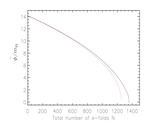
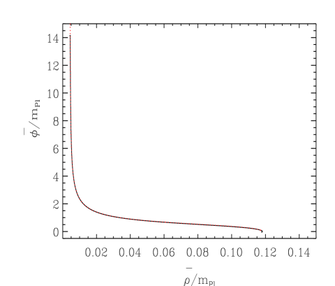
Figure 7: Same as in Fig. 6 but for different initial conditions. The parameters are $\alpha=\sqrt{2}$, $\beta=1$, $m=10^{-6}m_{{}_{\mathrm{P}l}}$, $\kappa A/(\alpha m)=1.35135$ and $W_{0}/A=0.41111$. This gives $y_{{\rm min},\tilde{\cal U}}\simeq 1.067$ or $\bar{\rho}_{{\rm min},\tilde{\cal U}}\simeq 0.004\times m_{{}_{\mathrm{P}l}}$. The absolute minimum of the potential is still located at $\phi=0$, $y=y_{{\rm min},\tilde{\cal V}}\simeq 1.622$ or $\bar{\phi}=0$, $\bar{\rho}=\bar{\rho}_{{\rm min},\tilde{\cal V}}\simeq 0.118\times m_{{}_{\mathrm{P}l}}$. The initial conditions are now $\phi_{\rm ini}=10\times m_{{}_{\mathrm{P}l}}$ or $\bar{\phi}_{\rm ini}\simeq 14.142\times m_{{}_{\mathrm{P}l}}$ and $y_{\rm ini}=y_{{\rm min},\tilde{\cal U}}\simeq 1.067$ or $\bar{\rho}_{\rm ini}=\bar{\rho}_{{\rm min},\tilde{\cal U}}\simeq 0.004\times m_{{}_{\mathrm{P}l}}$, i.e. still at the bottom of the valley exactly.

Our next step is to study whether the previous conclusions are robust and can be modified if we change either the initial conditions and/or the parameters of the model. In Fig. 7, we have considered another initial condition for the inflaton field, namely $\phi_{\rm ini}=10\times m_{{}_{\mathrm{P}l}}$ or $\bar{\phi}_{\rm ini}\simeq 14.142\times m_{{}_{\mathrm{P}l}}$, the other parameters being the same as in Fig. 6 [ i.e. $\alpha=\sqrt{2}$, $\beta=1$, $m=10^{-6}m_{{}_{\mathrm{P}l}}$, $\kappa A/(\alpha m)=1.35135$ and $W_{0}/A=0.41111$. The initial condition of the moduli waterfall field is $y_{\rm ini}=y_{{\rm min},\tilde{\cal U}}\simeq 1.067$ or $\bar{\rho}_{\rm ini}=\bar{\rho}_{{\rm min},\tilde{\cal U}}\simeq 0.004\times m_{{}_{\mathrm{P}l}}$, i.e. still at the bottom of the valley]. As can be seen all the remarks and conclusions obtained before remain valid for this case. Another remark is in order at this point. In the valley, since we have $V\sim\tilde{\cal U}\bar{\phi}^{2}$, the parameter $\delta_{\parallel}$ should vanish, see Eqs. (82) and (86). We see in Fig. 6 that, on the contrary, $\epsilon_{\parallel}$ and $\delta_{\parallel}$ are initially of the same order of magnitude, i.e. $10^{-3}$. The reason is that, initially, the two fields are not sufficiently “deep”in the valley. On the contrary, with the new initial condition $\bar{\phi}_{\rm ini}\simeq 14.142\times m_{{}_{\mathrm{P}l}}$, the fields are really in the straight part of the valley. As a consequence, one can check that the slow-roll parameter $\delta_{\parallel}$ ($\simeq 10^{-5}$) is now two orders of magnitude smaller than $\epsilon_{\parallel}$ ($\simeq 10^{-3}$), in full agreement with the arguments presented above. One can even check that the numerical values are consistent with the above interpretation. Indeed, as a time-dependent function, the slow-roll parameter $\epsilon$ is given by $\epsilon=m_{{}_{\mathrm{P}l}}^{2}/(4\pi\phi^{2})$. Therefore, initially one has $\epsilon=m_{{}_{\mathrm{P}l}}^{2}/(4\pi\phi_{\rm ini}^{2})\simeq 0.39\times 10^{-3}$ which is the value seen in Fig. 7 for small $N$.

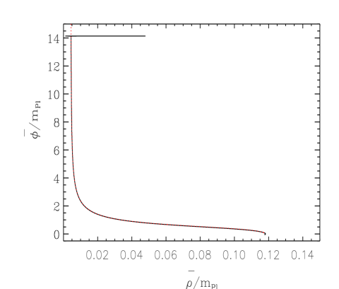
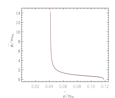
Figure 8: Left panel: inflationary trajectory in the case where the moduli does not start from the bottom of the valley. The parameters are $\alpha=\sqrt{2}$, $\beta=1$, $m=10^{-6}m_{{}_{\mathrm{P}l}}$, $\kappa A/(\alpha m)=1.35135$ and $W_{0}/A=0.41111$. The initial conditions are $\bar{\phi}_{\rm ini}=14.142\times m_{{}_{\mathrm{P}l}}$ and $\bar{\rho}_{\rm ini}=0.0479\times m_{{}_{\mathrm{P}l}}$. Right panel: inflationary trajectory for different values of the parameters characterizing the model. The parameters are $\alpha=\sqrt{2}$, $\beta=1$, $m=10^{-6}m_{{}_{\mathrm{P}l}}$, $\kappa A/(\alpha m)=1.30$ and $W_{0}/A=0.41111$, i.e. only the value of $A$ has been modified. As a consequence, the absolute minimum of the potential is still located at $\phi=0$, $y=y_{{\rm min},\tilde{\cal V}}\simeq 1.622$ or $\bar{\phi}=0$, $\bar{\rho}=\bar{\rho}_{{\rm min},\tilde{\cal V}}\simeq 0.118\times m_{{}_{\mathrm{P}l}}$ but the position of the valley is changed. It is now located at $\bar{\rho}=\bar{\rho}_{{\rm min},\tilde{\cal U}}\simeq 0.0415\times m_{{}_{\mathrm{P}l}}$. The initial conditions are $\phi_{\rm ini}=10\times m_{{}_{\mathrm{P}l}}$ or $\bar{\phi}_{\rm ini}\simeq 14.142\times m_{{}_{\mathrm{P}l}}$ and $y_{\rm ini}=y_{{\rm min},\tilde{\cal U}}\simeq 1.165$ or $\bar{\rho}_{\rm ini}=\bar{\rho}_{{\rm min},\tilde{\cal U}}\simeq 0.0415\times m_{{}_{\mathrm{P}l}}$, i.e. the field, in this case, still starts from the bottom of the valley exactly.

There exists another way of modifying the initial conditions. Instead of changing the initial value of the inflaton $\bar{\phi}$, we can also study what happens if the moduli field $\bar{\rho}$ is initially displaced from the bottom of the valley. This is especially relevant because it is known that hybrid inflation is very sensitive to the initial conditions and that only a very small fraction of possible initial conditions leads to successful inflation, see Refs. hybridini . In particular, it has been shown in these articles that the waterfall field must be precisely tuned at the bottom of the inflationary valley in order to obtain a satisfactory subsequent evolution. In Fig. 8 (left panel), we have used the same set of parameters as in the previous figures but the initial conditions are now $\bar{\phi}_{\rm ini}=14.142\times m_{{}_{\mathrm{P}l}}$ and $\bar{\rho}_{\rm ini}=0.0479\times m_{{}_{\mathrm{P}l}}$. The initial value of the moduli field is approximatively one order of magnitude larger than in Figs. 6 and 7. We see that successful inflation is still obtained. After very rapid oscillations, the moduli stabilizes at the bottom of the valley and then the evolution proceeds as before. Therefore, it seems that the present model is more stable to modifications of the initial conditions than standard hybrid inflation. Of course, what should really be done, as in Refs. hybridini , is a systematic scan of the space of initial conditions but this is beyond the scope of the present article.

Finally, we also need to study what happens if we change the parameters of the model, i.e. $A$ and $W_{0}$ (since $m$ is fixed by the CMB normalization). In Fig. 8 (right panel), the trajectory in the space $(\bar{\phi},\bar{\rho})$ is displayed for the following choice of parameters: $\alpha=\sqrt{2}$, $\beta=1$, $m=10^{-6}m_{{}_{\mathrm{P}l}}$, $\kappa A/(\alpha m)=1.30$ and $W_{0}/A=0.41111$. There is a new value for the parameter $A$ (and in fact a new value for $W_{0}$ but such that the ratio $W_{0}/A$ is left unchanged), of course still compatible with the constraints derived above. The position of the absolute minimum is unaffected because it only depends on $W_{0}/A$. On the other hand, the location of the valley (i.e. the location of the minimum of the mass function) is changed, since it depends on $\kappa A/(\alpha m)$ and is now located at $\bar{\rho}=\bar{\rho}_{{\rm min},\tilde{\cal U}}\simeq 0.0415\times m_{{}_{\mathrm{P}l}}$. We have chosen the initial conditions such that $\phi_{\rm ini}=10\times m_{{}_{\mathrm{P}l}}$ or $\bar{\phi}_{\rm ini}\simeq 14.142\times m_{{}_{\mathrm{P}l}}$ and such that the evolution starts from the (new) bottom of the valley exactly, namely $y_{\rm ini}=y_{{\rm min},\tilde{\cal U}}\simeq 1.165$ or $\bar{\rho}_{\rm ini}=\bar{\rho}_{{\rm min},\tilde{\cal U}}\simeq 0.0415\times m_{{}_{\mathrm{P}l}}$. We notice that the above conclusions remain unchanged: the fields follow the inflationary valley and join the absolute minimum of the potential as it was the case in the previous examples.

Our conclusion is that the main features of the mutated chaotic inflationary scenario seem to be robust either to modifications of the initial conditions or to changes of the parameters of the model, namely $A$ and/or $W_{0}$.

IV.8 Quantum stability

Let us finish this section by a discussion on the quantum stability of inflation along the valley where the inflaton rolls slowly. As can be seen in Fig. 4, the valley is bordered on each side by potential barriers. There is the infinite barrier at $\rho=0$ and a finite height barrier located at $y_{{\rm max},\tilde{\cal U}}$ defined as the second root of Eq. (54). Now this barrier separates the inflation valley and the vacuum at infinity with vanishing potential. There are two sources of instability of the valley. The first one is the tunneling of the moduli field through the barrier followed by the down roll towards $\rho=\infty$. The second one is stochastic evolution of the moduli field when its mass in the valley is much less than the Hubble rate. In our case, the mass of the moduli field is of the order of the Hubble rate implying that the moduli field is not light and does not fluctuate like a stochastic field with root mean square excursion $H/2\pi$. The only possibility for the moduli field to go through the barrier is tunneling. The tunneling time is approximated by the Coleman-De Luccia instanton coleman . In the thin-wall approximation where the height of the barrier is large, i.e. $\tilde{U}(y_{{\rm min},\tilde{\cal U}})/\tilde{U}(y_{{\rm max},\tilde{\cal U}})\ll 1$, and the width of the potential barrier is large in Planck units (see Fig. 3), the tunneling time is given by

$$t_{\rm Decay}\simeq t_{{}_{\rm Pl}}{\rm e}^{24m_{{}_{\mathrm{P}l}}^{4}\pi^{2}/V_{0}}\,,$$ (91)

where $V_{0}$ is the potential in the valley and $t_{{}_{\rm Pl}}$ the Planck time. Using $V_{0}\simeq 3m_{{}_{\mathrm{P}l}}^{2}H^{2}$ and $H\approx 10^{-6}m_{{}_{\mathrm{P}l}}$, one finds that the decay time is exponentially longer than the Planck time. For all practical purposes the valley is quantum stable. At the end of the evolution along the valley, the moduli becomes sensitive to the existence of the global minimum of the potential and rolls down the potential towards the global minimum.

V Mutated chaotic inflation and KKLT stabilization

In the previous section we have introduced a model of inflation with moduli stabilization and mutated chaotic inflation. Unfortunately, the vacuum energy at the end of inflation becomes negative. We have compensated this negative energy by introducing a constant and positive energy of unknown origin. Here, we will combine a string inspired stabilization mechanism (the KKLT stabilization mechanism) with mutated chaotic inflation. This is obtained by introducing an explicit moduli dependent potential which lifts the vacuum energy towards positive values.

V.1 Lifting AdS to dS

There are two equivalent ways of lifting the potential energy for the moduli. The first one comes from the D3/D7 system that we have already studied at the beginning of the previous section. Instead of studying the potential (43) in the vicinity of the minimum, which leads to Eq. (46), one can focus on the regime where the waterfall fields vanish $\phi^{\pm}=0$. Then, Eq. (43) leads to

$$V=\frac{2g^{2}\zeta^{4}}{\kappa^{3/2}\left(\rho+\rho^{\dagger}\right)^{3}}+\tilde{\cal V}(\rho)\,.$$ (92)

This is a KKLT potential with a correction term $\propto 1/\rho^{3}$, with a positive minimum provided $\zeta$ is chosen appropriately. However, we have already used the potential (43) to give a mass to the inflaton and, as discussed before, this was in another regime. Therefore, if we want to preserve this mechanism and stabilize the moduli by the KKLT method, the term $\propto 1/\rho^{3}$ must have another origin that we now discuss.

Assume that the model possesses a $U(1)$ gauge field with a Fayet–Iliopoulos term. The Kähler potential of the moduli is modified and becomes

$$K=-\frac{3}{\kappa}\ln\left[\kappa^{1/2}\left(\rho+\rho^{\dagger}\right)+\xi V\right]\,.$$ (93)

where $V$ is the vector superfield and $\xi$ is the Fayet–Iliopoulos term. This could be due to an anomalous symmetry cured by the Green-Schwarz mechanism. Moreover we assume that the gauge coupling function reads

$$f(\rho)=\frac{\kappa^{1/2}\rho}{\tilde{g}^{2}}\,,$$ (94)

where $\tilde{g}$ is a constant. Assuming that no field is charged under this $U(1)$ symmetry, the D-term associated to this gauge symmetry is

$$V_{{}_{\rm D}}=\frac{D}{\rho^{3}}\,,$$ (95)

where $D=\tilde{g}^{2}\xi^{2}/16$ Burgess2 . The total potential that we obtain is the potential of Eq. (43) plus $V_{{}_{\rm D}}$. Then, using our usual mechanism to give a mass to the inflaton and following the same step as before we find that the new potential reads

$$V\left(\rho,\phi\right)=\tilde{{\cal V}}(\rho)+\frac{D}{\rho^{3}}+\tilde{{\cal U}}(\rho)\phi^{2}\,.$$ (96)

We see that this only amounts to have a new offset function $\hat{{\cal V}}(\rho)\equiv\tilde{{\cal V}}(\rho)+D/\rho^{3}$. Hence, all the results obtained before on the mass function $\tilde{\cal U}$ are still valid.

V.2 KKLT stabilization and mutated chaotic inflation

Let us now discuss how the parameter $D$ can be fixed. We will not present a complete analysis of the parameter space as such an analysis is complicated. However, we will demonstrate that the KKLT mechanism also works in the case under consideration. The parameter $D$ must be chosen such that, at the absolute minimum of the potential, the potential exactly vanishes (or is equal to the value of the vacuum energy today. Since this one is tiny and since we only study the inflationary era, we will just assume that the minimum is zero). This means that we have to solve simultaneously the equations

$$y^{2}_{{\rm min},\hat{\cal V}}+\frac{7}{2}y_{{\rm min},\hat{\cal V}}+3=\frac{3W_{0}}{2A}{\rm e}^{y_{{\rm min},\hat{\cal V}}}\left(y_{{\rm min},\hat{\cal V}}+2\right)$$

$$-\frac{9D\kappa^{1/2}}{A^{2}}\frac{{\rm e}^{2y_{{\rm min},\hat{\cal V}}}}{y_{{\rm min},\hat{\cal V}}}\,,$$ (97)

$$\frac{{\rm e}^{-y_{{\rm min},\hat{\cal V}}}}{2y_{{\rm min},\hat{\cal V}}}\left[\frac{{\rm e}^{-y_{{\rm min},\hat{\cal V}}}}{3}-\frac{1}{y_{{\rm min},\hat{\cal V}}}\left(\frac{W_{0}}{A}-{\rm e}^{-y_{{\rm min},\hat{\cal V}}}\right)\right]$$

$$+\frac{\kappa^{1/2}D}{A^{2}y_{{\rm min},\hat{\cal V}}^{3}}=0\,.$$ (98)

The first condition is a condition on the derivative of the new offset function and is similar to Eq. (59) while the second equation is nothing but the condition that the potential is zero at the minimum. We see that the relevant new parameter is in fact the dimensionless quantity $\kappa^{1/2}D/A^{2}$.

Let us first consider the case where the parameters are $\alpha=\sqrt{2}$, $\beta=1$, $m=10^{-6}m_{{}_{\mathrm{P}l}}$, $W_{0}/A=0.4111$ and $\kappa A/(\alpha m)=1.35135$, i.e. the case envisaged before. Then, a solution to the two above equations can be found and reads: $\kappa^{1/2}D/A^{2}\simeq 0.027$ and $y_{{\rm min},\hat{\cal V}}\simeq 2.349$. The corresponding offset function is represented in Fig. 9 (solid line). One can check that there is indeed a minimum and that, at the minimum, the offset function vanishes. Let us now consider another case, namely $\alpha=\sqrt{2}$, $\beta=1$, $m=10^{-6}m_{{}_{\mathrm{P}l}}$, $W_{0}/A=1.2$ and $\kappa A/(\alpha m)=1.35135$, i.e. the value of the ratio $W_{0}/A$ is now different and, most importantly, greater than one. A solution can also be obtained and is: $\kappa^{1/2}D/A^{2}\simeq 0.145$ and $y_{{\rm min},\hat{\cal V}}\simeq 1.458$. The corresponding offset function is plotted in Fig. 9 (dotted line) and we check again that there is a vanishing minimum where the moduli can be stabilized. This case is in fact more interesting than the first one. Indeed, one sees that the ratio $W_{0}/A>1$ violates the bound established previously. Therefore, the KKLT mechanism allows us to find a vanishing minimum to the potential even if $W_{0}/A>1$. In other words, the constraint $W_{0}/A<1$ is relaxed.

Figure 9: Offset function obtained with the help of the KKLT stabilization mechanism. The solid line corresponds to the case $\alpha=\sqrt{2}$, $\beta=1$, $m=10^{-6}m_{{}_{\mathrm{P}l}}$, $W_{0}/A=0.4111$ and $\kappa A/(\alpha m)=1.35135$ and gives $\kappa^{1/2}D/A^{2}\simeq 0.027$ and $y_{{\rm min},\hat{\cal V}}\simeq 2.349$. The dotted line is obtained with the following set of parameters: $\alpha=\sqrt{2}$, $\beta=1$, $m=10^{-6}m_{{}_{\mathrm{P}l}}$, $W_{0}/A=1.2$ and $\kappa A/(\alpha m)=1.35135$, $\kappa^{1/2}D/A^{2}\simeq 0.145$ and the minimum is located at $y_{{\rm min},\hat{\cal V}}\simeq 1.458$.

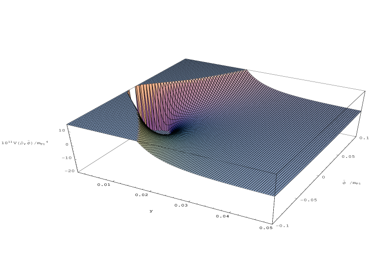
Figure 10: Potential without the KKLT term $D/\rho^{3}$ for the parameters: $\alpha=\sqrt{2}$, $\beta=1$, $m=10^{-6}m_{{}_{\mathrm{P}l}}$, $W_{0}/A=1.2$ and $\kappa A/(\alpha m)=1.35135$. Since $W_{0}/A>1$ the offset function has no minimum around $\bar{\phi}\simeq 0$, hence the “hole” that can be seen in this region. Let us also notice that the potential is plotted versus $y$ rather than versus $\bar{\rho}$ as it was the case in Fig. 4.

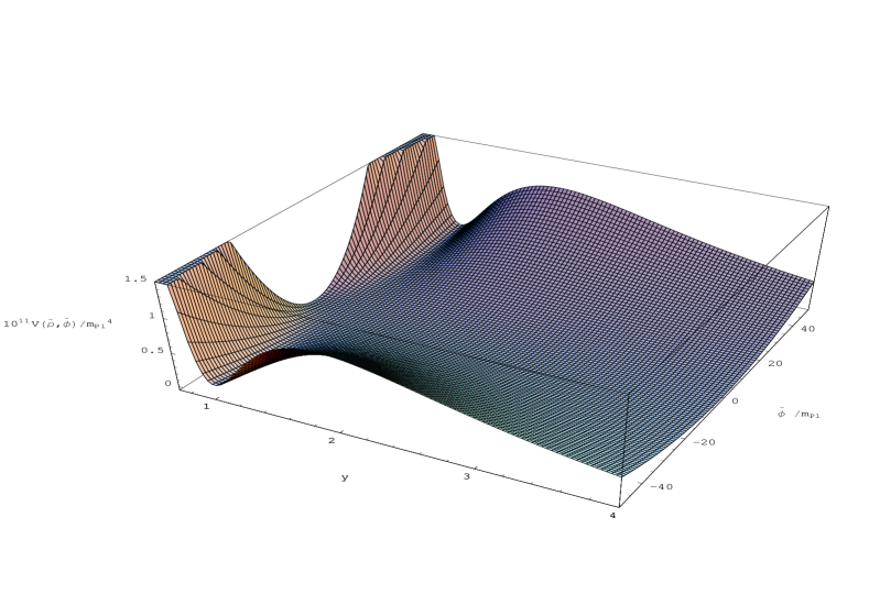
Figure 11: Potential with the KKLT term $D/\rho^{3}$ for the parameters: $\alpha=\sqrt{2}$, $\beta=1$, $m=10^{-6}m_{{}_{\mathrm{P}l}}$, $W_{0}/A=1.2$, $\kappa A/(\alpha m)=1.35135$ and $\kappa^{1/2}D/A^{2}\simeq 0.145$ (i.e. same set of parameters than in Fig. 10 but with a non–vanishing $D$). The fact that the moduli has been stabilized is obvious.

The above property is illustrated in Fig. 10 where we have plotted the potential $V(\bar{\rho},\bar{\phi})$ for the following set of parameters: $\alpha=\sqrt{2}$, $\beta=1$, $m=10^{-6}m_{{}_{\mathrm{P}l}}$, $W_{0}/A=1.2$, $\kappa A/(\alpha m)=1.35135$ and $\kappa^{1/2}D/A^{2}=0$. As already discussed above, the moduli cannot be stabilized in this case because $W_{0}/A>1$. The “hole” that can be seen in this figure represents the region of instability, i.e. the region where the offset function goes to $-\infty$. In Fig. 11, we have added the KKLT term $D/\rho^{3}$. The value of the parameters are $\alpha=\sqrt{2}$, $\beta=1$, $m=10^{-6}m_{{}_{\mathrm{P}l}}$, $W_{0}/A=1.2$, $\kappa A/(\alpha m)=1.35135$ and $\kappa^{1/2}D/A^{2}\simeq 0.145$, i.e. as for the dotted line in Fig. 9. The “hole” has now disappeared and the shape of the potential is very reminiscent to that of the potential studied in the previous subsection, see Fig. 4. In particular, it is clear that there is a new valley of stability.

It is now interesting to study the valley in more details. Since adding the term $D/\rho^{3}$ just amounts to modifying the form of the offset function, the analytical calculations which lead to the equation of the valley are very similar to those which resulted in Eq. (69). Straightforward manipulations yields

$$\kappa\phi^{2}_{\rm valley}\left(y\right) = \frac{4}{3}\left(\frac{\kappa A}{\alpha m}\right)^{2}y{\rm e}^{-2y}\left[y^{2}+\frac{7}{2}y+3-\frac{3}{2}\frac{W_{0}}{A}{\rm e}^{y}\left(y+2\right)+\frac{9\kappa^{1/2}D}{A^{2}}\frac{{\rm e}^{2y}}{y}\right]$$

$$\times\left[-\frac{3}{2}+2\left(\frac{\kappa A}{\alpha m}\right)y{\rm e}^{-y}+\left(\frac{\kappa A}{\alpha m}\right)y^{2}{\rm e}^{-y}\right]^{-1}\,.$$

As expected the only difference is the presence of the term proportional to $D$ at the numerator of the above equation. It is also interesting to give the trajectory expressed in terms of canonically normalized fields, i.e. the equivalent of Eq. (69). It can be expressed as

$$\kappa\bar{\phi}^{2}_{\rm valley}\left(\bar{\rho}\right) = \frac{8}{3}\left(\frac{\kappa A}{\alpha m}\right)^{2}\beta{\rm e}^{\sqrt{\frac{2}{3}}\kappa^{1/2}\bar{\rho}}\exp\left(-2\beta{\rm e}^{\sqrt{\frac{2}{3}}\kappa^{1/2}\bar{\rho}}\right)\biggl{[}\beta^{2}{\rm e}^{2\sqrt{\frac{2}{3}}\kappa^{1/2}\bar{\rho}}+\frac{7}{2}\beta{\rm e}^{\sqrt{\frac{2}{3}}\kappa^{1/2}\bar{\rho}}+3$$ (100)

$$- \frac{3}{2}\frac{W_{0}}{A}\exp\left(\beta{\rm e}^{\sqrt{\frac{2}{3}}\kappa^{1/2}\bar{\rho}}\right)\left(\beta{\rm e}^{\sqrt{\frac{2}{3}}\kappa^{1/2}\bar{\rho}}+2\right)+\frac{9\kappa^{1/2}D}{A^{2}\beta}{\rm e}^{-\sqrt{\frac{2}{3}}\kappa^{1/2}\bar{\rho}}\exp\left(2\beta{\rm e}^{\sqrt{\frac{2}{3}}\kappa^{1/2}\bar{\rho}}\right)\biggr{]}$$

$$\times \biggl{[}-\frac{3}{2}+2\left(\frac{\kappa A}{\alpha m}\right)\beta{\rm e}^{\sqrt{\frac{2}{3}}\kappa^{1/2}\bar{\rho}}\exp\left(-\beta{\rm e}^{\sqrt{\frac{2}{3}}\kappa^{1/2}\bar{\rho}}\right)+\left(\frac{\kappa A}{\alpha m}\right)\beta^{2}{\rm e}^{2\sqrt{\frac{2}{3}}\kappa^{1/2}\bar{\rho}}\exp\left(-\beta{\rm e}^{\sqrt{\frac{2}{3}}\kappa^{1/2}\bar{\rho}}\right)\biggr{]}^{-1}\,.$$

The valley is represented in Fig. 12 and compared to the valley obtained previously without the term $D/\rho^{3}$. As is clear form the figure, the two trajectories have the same features.

Figure 12: Trajectories of the valley of stability in the plan $(\bar{\rho},\bar{\phi})$ (the valley is seen from above). The solid line corresponds to the following parameters $\alpha=\sqrt{2}$, $\beta=1$, $m=10^{-6}m_{{}_{\mathrm{P}l}}$, $\kappa A/(\alpha m)=1.35135$ $W_{0}/A=0.41111$, $\kappa^{1/2}D/A^{2}=0$. There is no KKLT term in the potential and $W_{0}/A<1$. Therefore this is nothing but our “standard” case already displayed in Fig. 5. The dotted line represents the valley in the case where $\alpha=\sqrt{2}$, $\beta=1$, $m=10^{-6}m_{{}_{\mathrm{P}l}}$, $\kappa A/(\alpha m)=1.35135$ $W_{0}/A=1.2$, $\kappa^{1/2}D/A^{2}=0$, i.e. the KKLT term is still absent but the value of $W_{0}/A$ is now changed and is such that $W_{0}/A>1$. In this case the modulus is not stabilized and one sees the valley escaping to infinity. This case corresponds to Fig. 10. The fact that the valley goes to infinity is another manifestation of the “hole” that can be seen in Fig. 10. Finally, the dashed line represents the valley in the case where $\alpha=\sqrt{2}$, $\beta=1$, $m=10^{-6}m_{{}_{\mathrm{P}l}}$, $\kappa A/(\alpha m)=1.35135$ $W_{0}/A=1.2$ and $\kappa^{1/2}D/A^{2}=0.145$. This is the same case as before except that the KKLT is now present which allows us to have $W_{0}/A>1$. We see that the valley is now very similar to the one obtained before by simply adding a cosmological constant to the potential.

V.3 Numerical Results with KKLT stabilization

Our next step is to study the potential given by Eq. (96) numerically. The results are displayed in Fig. 13. This figure should be compared with Figs. 6 and 7 where the same quantities, i.e. $\bar{\phi}(N)$, $\bar{\rho}(N)$, $\bar{\phi}(\bar{\rho})$, $\epsilon_{\parallel}$, $\delta_{\parallel}$ and $m^{2}_{\perp}$, have also been displayed. The main conclusion that can be drawn from these plots is that the inflationary trajectory obtained in the case where the KKLT mechanism is responsible for the stabilization of the moduli is very similar to the trajectory obtained before (simply by adding a cosmological constant to renormalize the true vacuum). Therefore, all the properties that were discussed in the previous section are still valid in the present context.

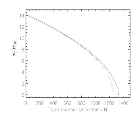
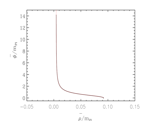
Figure 13: Same as Figs. 6 and 7 but with the KKLT mechanism taking into account. The parameters are $\alpha=\sqrt{2}$, $\beta=1$, $m=10^{-6}m_{{}_{\mathrm{P}l}}$, $\kappa A/(\alpha m)=1.35135$, $W_{0}/A=1.2$ and $\kappa^{1/2}D/A^{2}\simeq 0.145$. This gives $y_{{\rm min},\tilde{\cal U}}\simeq 1.067$ or $\bar{\rho}_{{\rm min},\tilde{\cal U}}\simeq 0.004\times m_{{}_{\mathrm{P}l}}$. The absolute minimum of the potential is located at $\phi=0$, $y=y_{{\rm min},\tilde{\cal V}}\simeq 1.457$ or $\bar{\phi}=0$, $\bar{\rho}=\bar{\rho}_{{\rm min},\tilde{\cal V}}\simeq 0.092\times m_{{}_{\mathrm{P}l}}$. The initial conditions are $\phi_{\rm ini}=10\times m_{{}_{\mathrm{P}l}}$ or $\bar{\phi}_{\rm ini}\simeq 14.142\times m_{{}_{\mathrm{P}l}}$ and $y_{\rm ini}=y_{{\rm min},\tilde{\cal U}}\simeq 1.067$ or $\bar{\rho}_{\rm ini}=\bar{\rho}_{{\rm min},\tilde{\cal U}}\simeq 0.004\times m_{{}_{\mathrm{P}l}}$, i.e. at the bottom of the valley exactly.

Let us now discuss in more details the inflationary scenario proposed in this article. Previously, we have studied the properties of the inflationary background only. However, it is clear that, if one wants to investigate all the consequences of the model, one must compare its predictions to the high accuracy cosmological data presently available in cosmology, in particular to the CMB data which are likely to carry an imprint from inflation. This requires the calculation of the cosmological perturbations and, in the present context, this is not a trivial task. The difficulty comes from the fact that we have more than one scalar field and hence the standard slow-roll single field result is not applicable here. In particular, we now have non-adiabatic perturbations. The non-adiabatic component is expected to be particularly important if the scales of astrophysical interest today left the Hubble radius in the “curved part” of the inflationary trajectory wr . This is the case, for instance, in Fig. 13 where $60$ e-folds before the end of inflation corresponds to a regime where the trajectory has already bent. To be more precise, it is quite easy to determine the spectral indices at Hubble crossing during inflation. They are simply given by the well-known equations wr

$$n_{{}_{\rm S}} = -4\epsilon_{\parallel}+2\delta_{\parallel}\,,$$ (101)

$$n_{{}_{\rm T}} = -2\epsilon_{\parallel}\,.$$ (102)

In these equations, $n_{{}_{\rm S}}$ is the spectral index of the adiabatic part of the density perturbations while $n_{{}_{\rm T}}$ is the tensor spectral index. One could have also given the spectral index of the isocurvature power spectrum but we do not need it here and it can be found in Ref. wr . We see that these formulae are a simple generalization of the one-field equations, $\epsilon_{\bar{\phi}}$ and $\delta_{\bar{\phi}}$ just being replaced by $\epsilon_{\parallel}$ and $\delta_{\parallel}$. We have computed $n_{{}_{\rm S}}$ and $n_{{}_{\rm T}}$ for some cases envisaged before, see Tab. 1.

	$\displaystyle\frac{W_{0}}{A}$	$\displaystyle\frac{\kappa A}{\alpha m}$	$\displaystyle\frac{\kappa^{1/2}D}{A^{2}}$	$\bar{\rho}_{{\rm min},\tilde{\cal U}}$	$\bar{\rho}_{{\rm min},\tilde{\cal V}}$	$\bar{\rho}_{\rm ini}$	$\bar{\phi}_{\rm ini}$	$N_{{}_{\rm T}}$	$n_{{}_{\rm S}}$	$n_{{}_{\rm T}}$
	$0.411$	$1.3513$	$0$	$0.004\times m_{{}_{\mathrm{P}l}}$	$0.118\times m_{{}_{\mathrm{P}l}}$	$0.004\times m_{{}_{\mathrm{P}l}}$	$14.142\times m_{{}_{\mathrm{P}l}}$	$1356$	$0.979$	$-0.012$
	$0.411$	$1.3513$	$0$	$0.004\times m_{{}_{\mathrm{P}l}}$	$0.118\times m_{{}_{\mathrm{P}l}}$	$0.004\times m_{{}_{\mathrm{P}l}}$	$4.242\times m_{{}_{\mathrm{P}l}}$	$161$	$0.979$	$-0.012$
	$1.2$	$1.3513$	$0.145$	$0.004\times m_{{}_{\mathrm{P}l}}$	$0.092\times m_{{}_{\mathrm{P}l}}$	$0.004\times m_{{}_{\mathrm{P}l}}$	$14.142\times m_{{}_{\mathrm{P}l}}$	$1331$	$0.974$	$-0.0139$
	$0.6$	$1.3513$	$0$	$0.004\times m_{{}_{\mathrm{P}l}}$	$0.008\times m_{{}_{\mathrm{P}l}}$	$0.004\times m_{{}_{\mathrm{P}l}}$	$14.142\times m_{{}_{\mathrm{P}l}}$	$1258$	$0.966$	$-0.0167$
	$0.411$	$1.330$	$0$	$0.017\times m_{{}_{\mathrm{P}l}}$	$0.118\times m_{{}_{\mathrm{P}l}}$	$0.017\times m_{{}_{\mathrm{P}l}}$	$14.142\times m_{{}_{\mathrm{P}l}}$	$1278$	$0.968$	$-0.0165$

Table 1: Spectral indices of the adiabatic scalar and tensor power spectra for different initial conditions and/or parameters $W_{0}/A$, $\kappa A/(\alpha m)$ and $\kappa^{1/2}D/A^{2}$. We also give the the minimums of the functions $\tilde{\cal V}$ and $\tilde{\cal U}$ as well as the initial conditions and the total number of e-folds predicted by the model.

These numbers must be compared with those obtained in the case of single field chaotic inflation (for a potential quadratic in the field),

$$n_{{}_{\rm S}}\simeq 0.967\,,\quad n_{{}_{\rm T}}\simeq-0.0165\,.$$ (103)

We see they are quite similar although not identical. In fact, the values of the spectral indices depend on the details of the inflationary trajectory. More precisely, what is important is how the trajectory is curved $N_{*}$ e-folds before the end of inflation. For instance, let us compare the cases corresponding to the two first columns in Tab. 1 to the cases corresponding to the two last columns. One can check that, for the two first cases, the inflationary trajectory is “more curved”, i.e. deviates from a straight line more strongly, than for the two last cases. As a consequence, the spectral indices obtained for the two first cases differ more from those obtained in the standard chaotic model than the spectral indices calculated in the two last cases do. Let us also remark that one could have expected a smaller difference in the case where the initial conditions are such that the fields start deep in the valley (i.e. , for instance, spectral indices closer to chaotic inflation in the case where $\bar{\phi}_{\rm ini}=14.142\times m_{{}_{\mathrm{P}l}}$ than for the case $\bar{\phi}_{\rm ini}=4.242\times m_{{}_{\mathrm{P}l}}$). However, what really matters is the value of the slow-roll parameters $N_{*}$ e-folds before the end of inflation and not at the beginning of inflation. Therefore, the previous reasoning does not work in our case, as confirmed by the numbers in Tab. 1. Finally, one notices that the differences observed are quite small and, although it seems easy to interpret them as we have just done above, we have not been able to find a simple criterion which would allow us to predict, from the values of the free parameters $W_{0}$, $A$ and $D$, how far from the fiducial model the spectral indices will be. It seems that this really depends on the fine structure of the valley near the Hubble scale exit.

As discussed in Ref. wr , the point is that the previous indices are not those that are observable. The reason is that the evolution of the perturbations after the Hubble radius exit during inflation is non trivial in presence of isocurvature perturbations. Technically, this is because the standard conserved quantity (on super-Hubble scales) $\zeta=-{\cal R}$ is sourced by the non-adiabatic pressure $\delta p_{\rm nad}$. The curvature and entropy perturbations evolve according to the equation

$$\begin{pmatrix}{\cal R}\cr{\cal S}\end{pmatrix}=\begin{pmatrix}1&T_{{\cal R}{\cal S}}\cr 0&T_{{\cal S}{\cal S}}\end{pmatrix}\begin{pmatrix}{\cal R}\cr{\cal S}\end{pmatrix}_{\rm exit}\,,$$ (104)

where the subscript “exit” means the corresponding quantities evaluated at the exit of the Hubble radius during inflation. They correspond to the quantities given in Tab. 1. Then, the next step consists in defining the correlation angle by wr

$$\cos\Delta\simeq\frac{T_{{\cal R}{\cal S}}}{\sqrt{1+T_{{\cal R}{\cal S}}^{2}}}\,,$$ (105)

which appears in the final expressions of the observable spectral indices (these expressions can be found in Ref. wr ). As shown in Ref. wr , the correlation angle is the only quantity needed in order to calculate the observable spectral indices from the directional slow-roll parameters introduced before. Unfortunately, this quantity is not easy to obtain. In the present context, this would require to numerically integrate the equations governing the evolution of the cosmological perturbations (and not only the equations governing the evolution of the background as done before). This is clearly beyond the scope of the present article. However, if $\Delta$ is not too far from $\pi/2$, then the estimates given in Tab. 1 are sufficient to demonstrate that the model seems to be presently compatible with the CMB data. We hope to address the question of determining the spectral indices exactly elsewhere. Let us finally notice that the value of the correlation angle has to be in agreement with the CMB constraints on the contribution originating from isocurvature perturbations obtained from the WMAP data, see for instance Ref. isowmap .

Another point worth discussing is the production of topological defects at the end of inflation. As was discussed recently in Ref. mairiJ , there exists quite tight constraints on the amount of cosmic string produced at the end of hybrid inflation. In the present context, this problem does not exist because the models studied here have only a single true vacuum. Hence, the production of topological defects at the end of inflation is simply not possible.

VI Conclusions

We now quickly summarize our main results. Firstly, we have emphasized the role that the shift symmetry plays in order to generate flat enough potentials in F–term inflation supergravity. Secondly, we have treated the issue of moduli stabilization and considered two different possibilities, namely a simple renormalization of the potential by a constant and the stringy motivated KKLT mechanism. Thirdly, we have combined the two above mentioned ingredients in order to construct inflationary models. We have shown that, quite generically, this gives rise to models that are reminiscent of mutated inflation where the inflationary path in the configuration space is non trivial. We have also demonstrated that, in these models, inflation ends by violation of the slow-roll conditions and not by instability as it is the case in standard hybrid inflation. Finally, we have pointed out that the calculations of cosmological perturbations may be non trivial due to the possible presence of non-adiabatic perturbations.

Acknowledgments

We wish to thank F. Quevedo for several interesting comments.

References

- (1) C. L. Bennet et al. , Astrophys. J. Suppl. 148, 1 (2003), astro-ph/0302207; G. Hinshaw et al. , Astrophys. J. Suppl. 148, 135 (2003), astro-ph/0302217; L. Verde et al. , Astrophys. J. Suppl. 148, 195 (2003), astro-ph/0302218; H. V. Peiris et al. Astrophys. J. Suppl. 148, 213 (2003), astro-ph/0302225; A. Kogut et al. , Astrophys. J. Suppl. 148, 161 (2003), astro-ph/0302213.
- (2) A. H. Guth, Phys. Rev. D 23, 347 (1981); A. D. Linde, Phys. Lett. B108, 389 (1982); A. Albrecht and P. J. Steinhardt, Phys. Rev. Lett. 48, 1220 (1982); A. Linde, Phys. Lett. B 129, 177 (1983).
- (3) V. Mukhanov and G. Chibisov, JETP Lett. 33, 532 (1981); Sov. Phys. JETP 56, 258 (1982); S. Hawking, Phys. Lett. 115B, 295 (1982); A. Starobinsky, Phys. Lett. 117B, 175 (1982); A. Guth and S.Y. Pi, Phys. Rev. Lett. 49, 1110 (1982); J. M. Bardeen, P. J. Steinhardt and M. S. Turner, Phys. Rev. D 28, 679 (1983).
- (4) V. F. Mukhanov, H. A. Feldman, and R. H. Brandenberger, Phys. Rep. 215, 203 (1992); J. E. Lidsey et al. , Rev. Mod. Phys. 69, 373 (1997), astro-ph/9508078; J. Martin and D. J. Schwarz, Phys. Rev. D57, 3302 (1998), gr-qc/9704049; J. Martin and D. J. Schwarz, Phys. Rev. D62, 103520 (2000), astro-ph/9912005; J. Martin, A. Riazuelo and D. J. Schwarz, Astrophys. J. 543, L99 (2000), astro-ph/0006392; D. J. Schwarz, C. A. Terrero-Escalante, and A. A. García, Phys. Lett. B 517, 243 (2001), astro-ph/0106020; S. M. Leach, A. R. Liddle, J. Martin and D. J. Schwarz, Phys. Rev. D66, 023515 (2002), astro-ph/0202094; J. Martin, Proceedings of the XXIV Brazilian National Meeting on Particles and Fields, Caxambu, Brazil, (2004), astro-ph/0312492; J. Martin, Lecture notes of the 40th Karpacz Winter School on Theoretical Physics, Poland, (2004), hep-th/0406011.
- (5) D. Lyth and A. Riotto, Phys. Rept. 314, 1 (1999), hep-ph/9807278.
- (6) N. Turok, M. Perry and P. J. Steinhardt, Phys. Rev. D70, 029901 (2005), hep-th/0408083; L. Cornalba and M. S. Costa, Fortsch. Phys. 52, 145 (2004), hep-th/0310099; B. Craps and B. A. Ovrut Phys. Rev. D69, 066001 (2004), hep-th/0308057; M. Berkooz and B. Pioline, JCAP 0311, 007 (2003), hep-th/0307280; L. Cornalba and M. S. Costa, Class. Quant. Grav. 20, 3969 (2003), hep-th/0302137; E. Dudas, J. Mourad and C. Timirgaziu, Nucl. Phys. B660, 3 (2003), hep-th/0209176; M. Fabinger and J. Mc Greevy, JHEP 0306, 042 (2003), hep-th/0206196; H. Liu, G. Moore and N. Seiberg, JHEP 0210, 031 (2002), hep-th/0206182; H. Liu, G. Moore and N. Seiberg, JHEP 0206, 045 (2002), hep-th/0204168; L. Cornalba and M. S. Costa, Phys. Rev. D66, 066001 (2002), hep-th/0203031; N. Ohta, Int. J. Mod. Phys. A20, 1 (2005), hep-th/0411230; U. H. Danielsson, hep-th/0409274.
- (7) M. Gasperini and G. Veneziano, Astropart. Phys. 1, 317 (1993); G. Veneziano, in The primordial Universe, Les Houches, session LXXI, edited by P. Binétruy et al., (EDP Science & Springer, Paris, 2000); M. Gasperini and G. Veneziano, Phys. Rep. 373, 1 (2003), hep-th/0207130.
- (8) J. Khoury, B. A. Ovrut, P. J. Steinhardt and N. Turok, Phys. Rev. D64, 123522 (2001), hep-th/0103239; J. Khoury, B. A. Ovrut, P. J. Steinhardt and N. Turok, hep-th/0105212; J. Khoury, B. A. Ovrut, N. Seiberg, P. J. Steinhardt and N. Turok, Phys. Rev. D65, 086007 (2002), hep-th/0108187; J. Khoury, B. A. Ovrut, P. J. Steinhardt and N. Turok, Phys. Rev. D66, 046005 (2002), hep-th/0109050; R. Durrer, hep-th/0112026; R. Kallosh, L. Kofman and A. Linde, Phys. Rev. D64, 123523 (2001), hep-th/0104073; R. Kallosh, L. Kofman, A. Linde and A. Tseytlin, Phys. Rev. D64, 123524 (2001), hep-th/0106241; D. H. Lyth, Phys. Lett. B 524, 1 (2002), hep-ph/0106153; R. H. Brandenberger and F. Finelli, JHEP 0111, 056 (2001), hep-th/0109004; J. Hwang, Phys. Rev. D65, 063514 (2002), astro-ph/0109045; D. H. Lyth, Phys. Lett. B 526, 173 (2002), hep-ph/0110007; J. Martin, P. Peter, N. Pinto-Neto and D. J. Schwarz, Phys. Rev. D65, 123513 (2002), hep-th/0112128; J. Martin and P. Peter, Phys. Rev. D68, 103517 (2003), hep-th/0307077. J. Martin and P. Peter, Phys. Rev. Lett. 92, 061301 (2004), astro-ph/0312488. J. Martin and P. Peter, Phys. Rev. D69, 107301 (2004), hep-th/0403173.
- (9) J. M. Cline, hep-th/0501179; C. P. Burgess, Pramana 63, 1269 (2004), hep-th/0408037; F. Quevedo, Class. Quant. Grav. 19, 5721 (2002), hep-th/0210292; C. P. Burgess, J. M. Cline, H. Stoica and F. Quevedo, JHEP 0409, 033 (2004), hep-th/0403119; C. P. Burgess, P. Martineau, F. Quevedo, G. Rajesh and R.-J. Zhang, JHEP 0203, 052 (2002), hep-th/0111025; C. P. Burgess, M. Majumdar, D. Nolte, F. Quevedo, G. Rajesh and R.-J. Zhang, JHEP 0107, 047 (2001), hep-th/0105204; N. Jones, H. Stoica and S. H. H. Tye, JHEP 0207, 051 (2002) hep-th/0203163, G. Shiu and S-H. H. Tye Phys. Lett. B513, 251 (2001), hep-th/0105307.
- (10) G. R. Dvali and S.-H. H. Tye, Phys. Lett. B450, 72 (1999), hep-ph/9812483.
- (11) H. Firouzjahi and S.-H. H. Tye. Phys. Lett. B584, 147 (2004), hep-th/0312020.
- (12) J. P. Hsu and R. Kallosh, JHEP 0404, 042 (2004), hep-th/0402047.
- (13) J. P. Hsu, R. Kallosh and S. Prokushkin, JCAP 0312, 009 (2003), hep-th/0311077.
- (14) K. Dasgupta, J. P. Hsu, R. Kallosh, A. Linde and M. Zagermann, JHEP 0408, 030 (2004), hep-th/0405247.
- (15) F. Koyama, Y. Tachikawa and T. Watari, Phys. Rev. D69 106001 (2004), hep-th/0311191.
- (16) S. Kachru, R. Kallosh, A. Linde and S. P. Trivedi, Phys. Rev. D68, 046005 (2003), hep-th/0301240.
- (17) C. P. Burgess, R. Kallosh and F. Quevedo, JHEP 0310, 056 (2003) hep-th/0309187.
- (18) K. Choi, A. Falkowski, H. P. Nilles and M. Olechowski, hep-th/0503216.
- (19) S. Kachru, R. Kallosh, A. Linde, J. Maldacena, L. Mc Allister and S. P. Trivedi, JCAP 0310, 013 (2003), hep-th/0308055.
- (20) L. Mc Allister hep-th/0502001.
- (21) M. Berg, M. Haack and B. Kors, Phys. Rev. D71, 026005 (2005), hep-th/0404087; M. Berg, M. Haack and B. Kors, contribution ot proceedings of “PASCOS’04”, hep-th/0409282.
- (22) J. J. Blanco–Pillado, C. P. Burgess, J. M. Cline, C. Escoda, M. Gomez–Reino, R. Kallosh, A. Linde and F. Quevedo, JHEP 0411 (2004) 063, hep-th/0406230.
- (23) W. H. Kinney, gr-qc/0503017.
- (24) A. Linde, Particle Physics and Inflationary Cosmology (Harwood Academic Publishers, Chur, Switzerland, 1990).
- (25) A. Linde, Phys. Lett. B259, 38 (1991); A. Linde, Phys. Rev. D49, 748 (1994), astro-ph/9307002; E. J. Copeland, A. R. Liddle, D. H. Lyth, E. D. Stewart and D. Wands, Phys. Rev. D49, 6410 (1994), astro-ph/9401011.
- (26) E. D. Stewart, Phys. Lett. B345, 414 (1995), astro-ph/9407040.
- (27) R. Jeannerot, S. Khalil, G. Lazarides and Q. Shafi, JHEP 0010, 012 (2000), hep-ph/0002151; R. Jeannerot, S. Khalil and G. Lazarides, JHEP 0207, 069 (2002), hep-ph/0207244.
- (28) S. Leach and A. R. Liddle, Phys. Rev. D68, 103503 (2003), astro-ph/0305263.
- (29) C. Gordon, D. Wands, B. A. Bassett and R. Maartens, Phys. Rev. D63, 023506 (2001), astro-ph/0009131; S. Groot Nibbelink and B. J. van Tent, Class. Quant. Grav. 19, 613 (2002), hep-ph/0107272; B. J. W. van Tent, Class. Quant. Grav. 21, 349 (2004), astro-ph/0307048.
- (30) G. Lazarides, C. Panagiotakopoulos and N. D. Vlachos, Phys. Rev. D54, 1369 (1996), hep-ph/9606297; G. Lazarides and N. D. Vlachos, Phys. Rev. D56, 4562 (1997), hep-ph/9707296; N. Tetradis, Phys. Rev. D57, 5997 (1998), astro-ph/9707214; L. E. Mendes and A. R. Liddle, Phys. Rev. D92, 103511 (2000), astro-ph/0006020.
- (31) S. Coleman and F. de Lucia, Phys. Rev. D21, 3305 (1980).
- (32) D. Wands, N. Bartolo, S. Matarrese and A. Riotto, Phys. Rev. D66, 043520 (2002), astro-ph/0205253.
- (33) K. Moodley, M. Bucher, J. Dunkley, P. G. Ferreira and C. Skordis, Phys. Rev. D70, 103520 (2004), astro-ph/0407304.
- (34) J. Rocher and M. Sakellariadou, hep-ph/0405133; J. Rocher and M. Sakellariadou, Phys. Rev. Lett. 94, 011303 (2005), hep-ph/0412143.