hep-th/0504164 April 2005(v1)

IITM/2005/PH/TH/2 June 2005(v2)

A quantum McKay correspondence for fractional $2p$-branes on LG orbifolds

Bobby Ezhuthachan

The Institute of Mathematical Sciences,
Chennai 600 113, India
Email: bobby@imsc.res.in

Suresh Govindarajan

Department of Physics, Indian Institute of Technology, Madras,
Chennai 600 036, India
Email: suresh@physics.iitm.ac.in
and

T. Jayaraman

Dept. of Mathematics,
Tata Institute of Fundamental Research,
Mumbai 400 005 India
Email: jayaram@theory.tifr.res.in

We study fractional $2p$-branes and their intersection numbers in non-compact orbifolds as well the continuation of these objects in Kähler moduli space to coherent sheaves in the corresponding smooth non-compact Calabi-Yau manifolds. We show that the restriction of these objects to compact Calabi-Yau hypersurfaces gives the new fractional branes in LG orbifolds constructed by Ashok et. al. in hep-th/0401135. We thus demonstrate the equivalence of the B-type branes corresponding to linear boundary conditions in LG orbifolds, originally constructed in hep-th/9907131, to a subset of those constructed in LG orbifolds using boundary fermions and matrix factorization of the world-sheet superpotential. The relationship between the coherent sheaves corresponding to the fractional two-branes leads to a generalization of the McKay correspondence that we call the quantum McKay correspondence due to a close parallel with the construction of branes on non-supersymmetric orbifolds. We also provide evidence that the boundary states associated to these branes in a conformal field theory description corresponds to a sub-class of the boundary states associated to the permutation branes in the Gepner model associated with the LG orbifold.

1 Introduction

During the past five years, our understanding of the spectrum of D-branes (both A and B-type) that appear in type II compactifications on Calabi-Yau(CY) manifolds has significantly improved. Some of the progress has been achieved by relating geometric constructions to non-geometric ones such as LG orbifolds and Gepner models. The first step in this context appeared in the [1] (see also [2] and [3] for a review). The method proposed for B-type D-branes was to analytically continue periods (identified with the central charge of D-branes) from non-geometric regions to geometric regions and then use this information to add geometric insight into the story. This method is rather tedious but it lead the way to a simpler picture for the large-volume analog of the Recknagel-Schomerus(RS) boundary states in the Gepner model[4]. From this emerged a connection with the McKay correspondence[7, 8, 9, 10, 11]. The RS boundary states turned out to be restriction of vector bundles or more generally coherent sheaves on the ambient (weighted) projective space to the CY hypersurface. However there are still several important aspects that are unclear and need to be clarified further. Among these is the question of an explicit description of B-type D-branes on Calabi-Yau manifolds that are not of this type.

A significant recent development in this direction has been the study of B-type D-branes at the Landau-Ginzburg(LG) point in the Kähler moduli space of a Calabi-Yau manifold. As one might, with hindsight, have expected from the simplicity of the LG theory, it is indeed possible to provide a fairly explicit description of B-type branes using boundary fermions and the technique of matrix factorization of polynomials[12]. This construction follows closely the conjecture of Kontsevich regarding the categorical description of B-type branes in the LG theory. In an interesting development it was shown in [13] that a new class of fractional branes can in fact be defined in the LG theory. The D-brane charges of these objects in terms of the charge basis at the large-volume point in Kähler moduli space have been computed.

Interestingly these fractional branes (in the LG description) include an object that corresponds at large volume to a single zero brane on the CY manifold. This is of particular interest since the Recknagel-Schomerus construction of boundary states in the Gepner model for CY manifolds appears to generically miss the D0-brane on the CY manifold. This D0-brane together with others that are related to it by the quantum symmetry at the LG point are of course only some examples of a large class of new branes that can be constructed using the technique of matrix factorization of the world-sheet superpotential of the LG Lagrangian.

This new approach to B-type branes in the LG theory is due to several authors [12, 13, 14, 15, 16]. For completeness we may mention another major development in this new approach has been the computation of the world-volume superpotential of such branes[17]. We also note that, from a purely mathematical point of view, there have been further developments in the categorical description of these B-type branes at the LG point and the derived equivalence of this category to the derived category of coherent sheaves on the same CY at large volume appears to have been established. This has been done in a series of papers by Orlov [18].

In this paper we will investigate the new fractional branes, referred to above, due to ref [13], by different methods without using the technique of matrix factorization and the introduction of boundary fermions. Our aim in particular, is to understand these states from a more transparently geometric point of view.

The key observation is that the new fractional branes essentially arise from considering Neumann type boundary conditions on the fields of the LG theory. In an earlier paper[2] it was observed that there were constraints on how Neumann boundary conditions could be imposed on the fields in the LG model in order to describe D-branes. There was a consistency condition involving the world-sheet superpotential. In the quintic we observed, for instance, that Neumann boundary conditions could be imposed only on linear combinations of LG fields and not on the individual fields themselves. This is very similar to the particular matrix factorization that ref. [13]) use in order to construct their new fractional branes.

Thus instead of the old fractional branes, which were fractional zero-branes, located at the singular point, we now consider fractional two-branes which are complex lines that pass through the fixed point. One may easily construct such objects in the orbifold theory without the world-sheet superpotential. The D-brane charges of these objects in the large volume basis can be computed by first determining the intersection of these fractional two-branes with the fractional zero-branes and with themselves. This can be easily done at the orbifold point. Subsequently, using these intersection numbers we can determine the large-volume charges of these fractional two-branes. It turns out that these fractional two-branes have a ‘fractional’ first Chern class. This fractional first Chern class ensures that when these objects are restricted to the CY hypersurface, one of them precisely becomes a zero-brane on the CY hypersurface. One may note that if we began with objects that have integer first Chern class on the ambient projective space then we would always obtain $d$ zero-branes on the CY hypersurface, where $d$ is the degree of the polynomial equation describing the CY.

Since the appearance of a ‘fractional’ first Chern class is somewhat surprising, we also show that these fractional two-branes have integer charges if we consider them as objects living in the ambient non-compact CY, which is a line bundle over a projective base, rather than on the projective space itself. In the Gauged Linear Sigma Model (GLSM) description, the true ambient space provided by the fields of the theory is in fact a non-compact CY. The CY itself comes from first restricting to the (weighted) projective space that is the base of the non-compact CY, and then restricting it to the appropriate hypersurface.

We also show that all the boundary states in the Ramond sector corresponding to the fractional two-branes can be described using the boundary conditions on the bulk world-sheet fermions. It was observed in [10] (see also [19]) that this in fact could be done for the fractional zero-branes themselves and in this paper we extend this observation to the new fractional branes.

For definiteness, we illustrate our method mainly in the case of the non-compact orbifold $\mathbb{C}^{3}/\mathbb{Z}_{3}$, the corresponding CY hypersurface being the elliptic curve given by a degree three equation in $\mathbb{P}^{2}$. The extension to the case of the quintic is straightforward. We note also that these fractional two-branes in non-compact orbifolds were earlier considered by Romelsberger[20] (for a discussion of the related boundary state construction see also [21]) and the appearance of a ‘fractional’ first Chern class was noted indirectly. This was explained there by the interplay of the relative homology of the ambient non-compact CY and the compact homology of the base projective space. Our description of the fractional two-branes in the ambient non-compact CY provides a clear toric description of the same phenomenon.

In this paper we also note a strong parallel between the relation of the fractional two-branes (and more generally fractional $2p$-branes) in the orbifold theory to the corresponding coherent sheaves at large volume and the notion of the quantum McKay correspondence due to Martinec and Moore [22]. While there is nothing quantum about the relation in our setting where space-time supersymmetry is not broken, nevertheless the fractional two-branes in $\mathbb{C}^{n}/\mathbb{Z}_{N}$ appear closely related to the fractional zero-branes of $\mathbb{C}^{n-1}/\mathbb{Z}_{N}$, the latter being the geometry associated with the non-supersymmetric B-type branes in the work of Martinec and Moore. In the full set of coherent sheaves that correspond to the quantum $\mathbb{Z}_{N}$ orbit of the fractional two-branes at large volume we are able to find the analogues of the so-called ‘Coulomb branes’ that they describe.

Finally we also identify the CFT description of states of the LG model that correspond to fractional two-brane and four-brane states in the ambient non-compact orbifold that are restricted to the CY hypersurface. This turns out to be a sub-class of the B-type permutation branes of the Gepner models that have been studied earlier[23].

The organization of the paper is as follows: In section 2, we discuss the background to the paper and explain the setting of the problem. In particular, we focus on linear boundary conditions in LG orbifolds. Using the GLSM, section 3 gives a heuristic derivation of the large volume analogs of D-branes for a specific set of boundary conditions in the LG orbifold for the Fermat quintic. We provide evidence that these are indeed the new fractional branes obtained in the first reference[13]. In section 4, we focus on fractional $2p$-branes in orbifolds of $\mathbb{C}^{n}/\mathbb{Z}_{N}$, in order to better understand the results of section 3. We work out a master formula, Eq. (4.14), for the intersection forms at the orbifold. These intersection forms are independently computed in the large volume as well. The case of $\mathbb{C}^{3}/\mathbb{Z}_{3}$ is worked out in some detail. Section 5 discusses how, for instance, fractional two-branes in a supersymmetric orbifold $\mathbb{C}^{n}/\mathbb{Z}_{N}$ are related to fractional zero-branes on a related non-supersymmetric orbifold $\mathbb{C}^{n-1}/\mathbb{Z}_{N}$. We argue for the existence of a quantum McKay correspondence which relates sheaves associated with fractional $2p$-branes on $\mathbb{C}^{n}/\mathbb{Z}_{N}$ to the sheaves associated with tautological bundles for $(2n\!-\!2p)$-branes on the same orbifold. Section 6 connects our results in the LG orbifold with boundary conformal field theory. We provide evidence that the fractional two-branes and a certain class of fractional four-branes on restriction to the compact Calabi-Yau hypersurface are given by a sub-class of the permutation branes constructed in the Gepner model[23]. We conclude in section 7 with a summary of our results and some comments on unresolved issues. The appendices have been used to collect several technical results.

While this work was being readied for publication, a paper [24] appeared and has substantial overlap with the results in section 6.

2 Background

2.1 Gepner models, LG orbifolds and the GLSM

Consider a Gepner model obtained by tensoring of $n$ $N=2$ minimal models of level $k_{i}$, $i=1,\ldots,n$. The total central charge of the model is

$$\hat{c}=\sum_{i=1}^{n}\frac{k_{i}}{k_{i}+2}=m$$

The related LG orbifold is obtained by considering $n$ chiral superfields(notation as in refs. [25, 26, 7]) $\Phi_{i}$ with a $\mathbb{Z}_{K}$ action ($K\equiv\textrm{lcm}(k_{1},\ldots,k_{n})$):

$$\mathbb{Z}_{K}:\quad\Phi_{i}\rightarrow\omega^{Q_{i}}\ \Phi_{i}\quad,$$

where $\omega=\exp(i2\pi/K)$ is a $K$-th root of unity and $Q_{i}\equiv K/(k_{i}+2)$. The model has a quasi-homogeneous superpotential given by

$$G(\Phi)=\sum_{i=1}^{n}\Phi^{k_{i}+2}\ .$$ (2.1)

We will be focusing mainly on the case when $n=m+2$ for which $K=\sum_{i}Q_{i}$.

The LG orbifold can be obtained as a ‘phase’ of a gauged linear sigma model (GLSM) by coupling the chiral fields to an abelian vector multiplet as well as another chiral multiplet $P$. The charges of the $n$ chiral multiplets under this $U(1)$ are $Q_{i}$ and the chiral multiplet $P$ has charge $-K$. The D-term constraint is

$$\sum_{i=1}^{n}Q_{i}|\phi_{i}|^{2}-K|p|^{2}=r\ ,$$ (2.2)

where $r$ is the Fayet-Iliopoulos(FI) parameter. The superpotential in the GLSM is taken to be

$$W(\Phi,P)=P\ G(\Phi)\ ,$$

where $G(\Phi)$ as defined in Eq. (2.1).

When $r\ll 0$, the $p$ field is non-zero in the ground state and the $U(1)$ is broken to $\mathbb{Z}_{K}$. Further, the fluctuations of the $p$ field are massive and can be integrated out to obtain the LG orbifold. When $r\gg 0$, not all the $\phi_{i}$ can vanish simultaneously and $p=0$ in the ground state. The $\phi_{i}$ become homogeneous coordinates on a weighted projective space $\mathbb{P}^{n-1}[Q_{i}]$ with weights $Q_{i}$. The equation of motion of the $p$ field imposes the restriction that the fields $\phi_{i}$ lie on the hypersurface $G=0$ in $\mathbb{P}^{n-1}[Q_{i}]$. In the absence of the superpotential, one obtains the total space of the line bundle ${\cal O}(-K)$ as the moduli space with the $\mathbb{P}^{n-1}[Q_{i}]$ being given by the condition $p=0$. i.e., the zero section of the line bundle.

2.2 Linear boundary conditions in LG orbifolds

Now consider the LG orbifold on a worldsheet with boundary preserving $B$-type supersymmetry. Such boundary conditions were studied in [2], where it was shown that linear boundary conditions are specified by a hermitian matrix $B$ which squares to identity, $B^{2}=1$ and is block diagonal (it mixes fields with identical charges). The boundary conditions then take the form

$${\big{(}P_{D}\big{)}_{i}}^{j}\ \phi_{j}=0 {\big{(}P_{D}\big{)}_{i}}^{j}\ \tau_{j}=0$$ ,

$${\big{(}P_{N}\big{)}_{i}}^{j}\ \xi_{j}=0 {\big{(}P_{N}\big{)}_{i}}^{j}\ \partial_{n}\phi_{j}=0$$ , (2.3)

where $\xi_{i}\equiv(\psi_{+i}+\psi_{-i})/\sqrt{2}$ and $\tau_{i}\equiv(\psi_{+i}-\psi_{-i})/\sqrt{2}$. The matrices $P_{N}\equiv(1+B)/2$ and $P_{D}\equiv(1-B)/2$ project onto the Neumann and Dirichlet directions respectively. The matrix $B$ which specifies the boundary conditions needs to satisfy an additional condition due to the presence of the superpotential in the LG model

$$\frac{\partial G}{\partial\phi_{i}}\ {\big{(}P_{N}\big{)}_{i}}^{j}=0\ .$$ (2.4)

In simple models involving a single chiral field, the only possible condition is the Dirichlet one. This carries over to the case of several chiral superfields when one imposes boundary conditions separately on each of the chiral superfields, i.e., the matrix $B$ is taken to be diagonal. For LG orbifolds associated with Gepner models, this implies that all the boundary states constructed by Recknagel and Schomerus in [4] must necessarily arise from Dirichlet conditions being imposed on all the chiral superfields. Further, when the superpotential is degenerate at $\phi_{i}=0$, the condition $G=0$ implies that the RS states arise from the boundary condition $\phi_{i}=0$ for all $i$.

2.3 Relating to D-branes at large volume

Based on the results for the $\mathbb{C}^{3}/\mathbb{Z}_{3}$ orbifold[6], it was conjectured in [7] that the fractional zero-branes on $\mathbb{C}^{n}/\Gamma$ (with $\Gamma$ a discrete abelian subgroup of $SU(n)$) correspond at large volume to (exceptional) coherent sheaves that provide a natural basis for bundles on the exceptional divisor of the (possibly partial) resolution of $\mathbb{C}^{n}/\Gamma$. A second conjecture in [7] was that the RS boundary states (to be precise, the $L_{i}=0$ RS states) were given by the restriction of the fractional zero-branes to the Calabi-Yau hypersurface. Substantial evidence for this was provided in refs. [8, 9, 10].

While the exceptional coherent sheaves obtained from fractional zero-branes do provide a basis for sheaves on the exceptional divisor of the resolution, this does not remain true on restriction to the Calabi-Yau threefold. For the case of the quintic, one finds that the bundles that are obtained by restriction span an index-25 sub-lattice of the lattice of RR charges of the quintic. In particular, the zero-brane and two-brane charges appear in multiples of 5 of the smallest possible value[7, 28]. This suggests that one must generalise the Recknagel-Schomerus construction to obtain new boundary states in the Gepner model or equivalently consider more general boundary conditions in the LG orbifold. As was explained in the previous subsection, the RS boundary states correspond to imposing Dirichlet boundary conditions on all the fields in the LG orbifold. It is thus natural to consider boundary conditions that impose Neumann boundary conditions on one or more linear combinations of fields as given in Eq. (2.3). For instance, for the LG orbifold for the superpotential given by the Fermat quintic, one such boundary condition is (see sec. 3.3.3 of [2])

$$(\phi_{1}+\phi_{2})=0 \phi_{i}=0\quad\textrm{for }i=3,4,5\ ,$$ ,

$$(\xi_{1}-\xi_{2}) = 0$$ (2.5)

It is easy to see that the above boundary conditions satisfy the constraint (2.4) or equivalently that $G=0$ on the boundary. Such branes will be referred to as fractional two-branes. We will see that restriction of one of the fractional two-branes to the quintic hypersurface leads to a zero-brane of minimal charge.

3 Fractional two-branes: the quintic in $\mathbb{P}^{4}$

In this section, we will provide a heuristic derivation of the identity, at large volume, of the D-branes associated with the boundary conditions given in Eq. (2.5). As with any heuristic derivation, we will not provide complete justification but only a motivation for some of the steps involved. Nevertheless, at the end of the derivation, we will have concrete candidates for the identity of the new D-branes. These new D-branes will be shown to have the same intersection numbers as those of the new fractional branes proposed in [13]. We will also provide further justification for the heuristic derivation in the section 4. This, we believe, provides geometric insight into the categorical construction of [13] in addition to identifying two apparently distinct approaches to D-branes on LG orbifolds. For purposes of illustration, we first consider the case of the original fractional zero-branes.

3.1 Fractional zero-branes from Euler sequences

As has already been mentioned, the original fractional branes (to be identified with the Recknagel-Schomerus states) are obtained by imposing Dirichlet boundary conditions on all fields in the LG orbifold. This leaves us with five independent fermionic multiplets on the boundary (the bulk chiral multiplet splits up into a fermionic multiplet and a chiral multiplet on the boundary) We will use the GLSM to interpolate between the LG orbifold and the nonlinear sigma model(NLSM).

The simplest way to obtain the LG orbifold from the GLSM is to consider the limit $e^{2}r\rightarrow-\infty$. In this limit, the fields in the vector multiplet behave as Lagrange multipliers. The $D$-field imposes the $D$-term constraints and the gauginos impose the constraint[26]:

$$\sum_{i}Q_{i}\phi_{i}\bar{\psi}_{\pm i}=0\ .$$

For the case of the LG model with boundary, when one imposes Dirichlet boundary conditions on all fields, this equation imposes a condition on the fermionic combination $\bar{\xi}_{i}$ that is not set to zero by the boundary conditions. Thus, the gaugino constraint on the boundary is now

$$\sum_{i}Q_{i}\phi_{i}\bar{\xi}_{i}=0$$ (3.1)

It is important to what follows that these fermions $\xi_{i}$ play the role of the boundary fermions that are used to construct coherent sheaves associated with B-type branes at large volume. The argument for this is based on two observations. First, the six-brane is one of the Recknagel-Schomerus states and hence arises from having Dirichlet boundary conditions on all the fields in the case of the LG orbifold. This implies that in analytically continuing (in Kähler moduli space) the D-branes from the LG orbifold to the large volume limit, all Dirichlet boundary conditions become Neumann boundary conditions (see also the discussion in [26]). Second, in the GLSM construction that realises B-type branes as coherent sheaves, the boundary condition at large volume relates the $\xi_{i}$ to the boundary fermions $\pi_{a}$ via the boundary condition[19]

$$\bar{\xi}_{i}=i\frac{\partial J^{a}}{\partial\phi_{i}}\pi_{a}$$ (3.2)

$J^{a}(\phi)$ ($a=1,\ldots,r$) are $r$ homogeneous polynomials of degree $d$. This boundary condition appears for the coherent sheaf given by the following exact sequence

$$0\rightarrow E\rightarrow{\cal O}^{\oplus r}\stackrel{{\scriptstyle J}}{{\rightarrow}}{\cal O}(d)\rightarrow 0$$

which corresponds to imposing the holomorphic constraint $J^{a}\pi_{a}=0$ on $r$ fermions, $\pi_{a}$ ($a=1,\ldots,r$). considered as sections of ${\cal O}^{\oplus r}$. Treating the gaugino constraint in Eq. (3.1) as a degree one holomorphic constraint, that is setting $J^{a}\equiv\phi^{a}$ we obtain the Euler sequence on $\mathbb{P}^{4}$

$$0\rightarrow\Omega(1)\rightarrow{\cal O}^{\oplus 5}\rightarrow{\cal O}(1)\rightarrow 0$$

with the boundary condition

$$\bar{\xi}_{i}=i\pi_{i}\ .$$

Thus, one can indeed bypass the introduction of boundary fermions by treating the $\bar{\xi}_{i}$ as boundary fermions and the gaugino constraint as a holomorphic constraint.

Of course, we have five boundary states associated with the LG orbifold. It turns out that the other four coherent sheaves are given by the following exact sequences that can be derived from the Euler sequence (given for $\mathbb{P}^{n}$ below though we only need the case of $n=4$ here) associated with $\Omega^{p}(p)\equiv\wedge^{p}\Omega\otimes{\cal O}(p)$

$$0\rightarrow\Omega^{p}(p)\rightarrow{\cal O}^{\oplus({}^{n+1}_{~{}p})}\rightarrow\Omega^{p-1}(p-1)\otimes{\cal O}(1)\rightarrow 0$$ (3.3)

Note the appearance of the binomial coefficients $({}^{n+1}_{~{}p})$ in the above sequences.

The boundary fermion construction naturally leads to the spinor bundle on $E$ rather than the coherent sheaf $E$. In the GLSM construction to obtain just the coherent sheaf we restrict to one-particle states in the corresponding boundary state. It was observed in [19] (see sec. 5.3) that when $E$ is the cotangent bundle, the spinor bundle decomposes at different fermion numbers to the different fractional branes. Thus, the monodromy about the LG point is realised by suitably changing the restriction on the fermion number of the states. Thus, the five fractional branes for the quintic are in one-to-one correspondence with the states: (the vacuum $|0\rangle$ satisfies $\bar{\xi}_{i}|0\rangle=0$)

$$|0\rangle\quad,\quad\xi_{i}|0\rangle\quad,\quad\xi_{i}\xi_{j}|0\rangle\quad,\quad\xi_{i}\xi_{j}\xi_{k}|0\rangle\quad,\quad\xi_{i}\xi_{j}\xi_{k}\xi_{l}|0\rangle$$

subject to the condition $\phi_{i}\bar{\xi}^{i}=0$ being imposed. (A related observation was made by Mayr in [10] where he referred to the fractional branes as providing a fermionic basis for branes).

We define (using the notation in [13])

$$\boxed{{\cal M}_{i}\equiv(-)^{i}\Omega_{\mathbb{P}^{4}}^{i}(i)\Big{|}_{\textrm{quintic}}\quad,\ i=0,1,2,3,4}$$ (3.4)

These branes ${\cal M}_{i}$ can be identified as the result of the analytic continuation to large-volume of the RS states in the Gepner model for the quintic. Under the quantum $\mathbb{Z}_{5}$ symmetry(generated by $g$), one has

$$g:\quad{\cal M}_{i}\rightarrow{\cal M}_{i+1\textrm{ mod }5}$$

A basic test of this identification is based on the idea that we expect the intersections of these branes (which is a topological quantity computed by the open-string Witten index) to be the same at the orbifold point and at large volume. At the orbifold point the intersections can be readily computed from CFT techniques. For coherent sheaves on a smooth CY we can compute the intersections using standard methods from differential geometry. The two must agree and they indeed do so for the $L_{i}\equiv 0$ states from among the RS states in the Gepner model and the ${\cal M}_{i}$ that we have just described above.

3.2 Fractional two-branes from generalised Euler sequences

We are now ready to discuss the case of fractional two-branes. As we have already seen, the Neumann boundary condition on the combination $(\phi_{1}-\phi_{2})$ is obtained from the supersymmetric variation of the boundary condition $\xi_{1}=\xi_{2}$. Thus, on the boundary, given these boundary conditions, we have effectively four independent fermionic multiplets. These fermionic multiplets are still subject to the condition (3.1) imposed by the gaugino. After eliminating $\bar{\xi}_{2}$ in favour of $\bar{\xi}_{1}$ using Eq. (2.5), Eq. (3.1) can be re-written as the following condition

$$\big{(}\phi_{1}+\phi_{2})\bar{\xi}_{1}+\sum_{i=3}^{5}\phi_{i}\bar{\xi}_{i}=0$$ (3.5)

Thus, this is equivalent to having four boundary fermions subject to the one condition above. Unlike the case of fractional zero-branes, we see that Eq. (3.5) is trivially satisfied when $\phi_{1}+\phi_{2}=\phi_{3}=\phi_{4}=\phi_{5}=0$. This is possible on $\mathbb{P}^{4}$, when $\phi_{1}-\phi_{2}\neq 0$. Note that these conditions specify a two-brane (denoted below by $P$) in the manifold which is the resolution of the $\mathbb{C}^{5}/\mathbb{Z}_{5}$ singularity. It is trivial to see that this two-brane restricts to a point on the quintic. Away from the two-brane $P$, Eq. (3.5) does reduce the number of fermions to three. This implies that the fermions are sections of the sheaf $F_{1}$ given by the following sequence

$$0\rightarrow F_{1}\rightarrow{\cal O}^{\oplus 4}\rightarrow{\cal O}(1)\rightarrow{\cal X}_{P}\rightarrow 0$$ (3.6)

The term involving ${\cal X}_{P}$ has been added to take care of the fact that (3.5) is trivially satisfied on $P$. The following comments are in order here:

1. ${\cal X}_{P}$, by definition, vanishes away from $P$. In particular, it vanishes on the $\mathbb{P}^{3}\in\mathbb{P}^{4}$ where $(\phi_{1}-\phi_{2})=0$.

2. Defining

   $$0\rightarrow F_{0}\rightarrow{\cal O}\rightarrow{\cal X}_{P}\otimes{\cal O}(-1)\rightarrow 0\ ,$$

   the sequence can be rewritten as

   $$0\rightarrow F_{1}\rightarrow{\cal O}^{\oplus 4}\rightarrow F_{0}\otimes{\cal O}(1)\rightarrow 0$$ (3.7)

3. $F_{0}$ restricts to ${\cal O}_{\mathbb{P}^{3}}$ on the $\mathbb{P}^{3}$ not containing $P$.

4. The above sequence when restricted to the $\mathbb{P}^{3}$ not containing $P$ becomes the Euler sequence. Thus $F_{1}|_{\mathbb{P}^{3}}=\Omega_{\mathbb{P}^{3}}^{1}(1)$.

5. Note that $F_{1}$ is however a sheaf on $\mathbb{P}^{4}$ even though the sequence which generates it is reminiscent of the Euler sequence for $\mathbb{P}^{3}$.

The above identification suggests that the remaining fractional branes can be given by exact sequences that on restriction to a $\mathbb{P}^{3}$ not containing $P$ give the generalised Euler sequences of $\mathbb{P}^{3}$. Explicitly, we can write

$$0\rightarrow F_{0}\rightarrow{\cal O}\rightarrow{\cal X}_{P}\otimes{\cal O}(-1)\rightarrow 0$$

$$0\rightarrow F_{1}\rightarrow{\cal O}^{\oplus 4}\rightarrow F_{0}\otimes{\cal O}(1)\rightarrow 0$$

$$0\rightarrow F_{2}\rightarrow{\cal O}^{\oplus 6}\rightarrow F_{1}\otimes{\cal O}(1)\rightarrow 0$$ (3.8)

$$0\rightarrow F_{3}\rightarrow{\cal O}^{\oplus 4}\rightarrow F_{2}\otimes{\cal O}(1)\rightarrow 0$$

$$0\rightarrow F_{4}\rightarrow{\cal O}\rightarrow F_{3}\otimes{\cal O}(1)\rightarrow 0$$

The last sequence which generates $F_{4}$ is rather interesting. One can argue that $F_{4}=-{\cal X}_{P}\otimes{\cal O}(3)$. That $F_{4}$ must at least have ${\cal X}_{P}$ as a factor is clear since the last sequence must restrict to zero on on the $\mathbb{P}^{3}\in\mathbb{P}^{4}$ not containing $P$. This is because there is no corresponding generalized Euler sequence that appears on $\mathbb{P}^{3}$. The factor of ${\cal O}(3)$ can be deduced from the general pattern that we observe in these sequences. We refer to $F_{4}$ as the Coulomb branch brane because of this vanishing property on restriction to the $\mathbb{P}^{3}$ not containing $P$. The remaining branes $(F_{0},\ldots,F_{3})$ will be called as the Higgs branch branes. As will be explained later, this parallels the missing branes that one needed to make a correspondence (called the quantum McKay correspondence) between D-branes on a non-supersymmetric orbifold and D-branes on the Hirzebruch-Jung resolution as considered by Martinec and Moore[22]. This relationship will be made more precise in a later section.

The main claim we wish to make is that the new fractional branes of [13] are to be identified with (a minus sign indicates an anti-brane)

$$\boxed{{\cal F}_{i}=(-)^{i}F_{i}\Big{|}_{\textrm{quintic}}\ ,\quad i=0,1,2,3,4}$$ (3.9)

provided we choose

$$\textrm{ch}\ \big{(}{\cal X}_{P}\big{)}\big{|}_{\textrm{quintic}}=J^{3}/5\ .$$ (3.10)

where $J$ generates the Kähler class on the quintic and is normalised such that $\langle J^{3}\rangle_{\textrm{quintic}}=5\langle J^{4}\rangle_{\mathbb{P}^{4}}=5$. As a first check, we have verified that the Chern classes of the ${\cal F}_{i}$ agree with those given by Ashok et. al. in [13]. (More details are provided in appendix A.) We also propose that under the quantum $\mathbb{Z}_{5}$ symmetry, one has

$$g:\quad{\cal F}_{i}\rightarrow{\cal F}_{i+1\textrm{ mod }5}$$

We will motivate here this unusual assignment of Chern character for the object ${\cal X}_{P}$ while a more detailed justification of the appearance of the $1/5$ factor will be provided in a later section. It is clear from a simple argument that sheaves in the ambient projective space (obtained from the fractional branes by blowing up the orbifold singularity) when restricted to the Calabi-Yau would fail to give objects that have the charge of a single zero-brane on the CY. A two-brane wrapping a $\mathbb{P}^{1}\in\mathbb{P}^{4}$ (which intersects the quintic on a point) will have Chern character $J^{3}+aJ^{4}$ for some $a$. On restricting this to the quintic, we obtain an object with Chern character $J^{3}$ which has the charge of $5$ zero-branes. Thus if we need to produce an object with the charge of a single zero-brane on the CY it appears that we must begin with a sheaf on $\mathbb{P}^{4}$ whose Chern character has leads off with a $J^{3}/5$ term. However more is clearly needed to justify this unusual choice.

Note that with this assignment of fractional Chern characters to the object ${\cal X}_{P}$ the maps in the exact sequences for the $F_{i}$ that we have given no longer have any obvious and rigorous mathematical meaning. This is in contrast to the case of the large-volume analogs of the fractional zero-branes that we discussed earlier where this a clear correspondence between physical constructions in the GLSM and rigourous mathematical constructions. Nevertheless we will continue to use these exact sequences for the $F_{i}$’s at least as a convenient device or a mnemonic to write down their Chern characters and hence their D-brane charges.

The five new fractional two branes for the quintic are in one-to-one correspondence with the states: (the vacuum $|0\rangle$ satisfies $\bar{\xi}_{i}|0\rangle=0$ and $i=1,3,4,5$ below)

$$F_{0}\sim|0\rangle\ ,\quad F_{1}\sim\xi_{i}|0\rangle\ ,\quad F_{2}\sim\xi_{i}\xi_{j}|0\rangle\ ,\quad F_{3}\sim\xi_{i}\xi_{j}\xi_{k}|0\rangle\ ,\quad F_{4}\sim\xi_{1}\xi_{3}\xi_{4}\xi_{5}|0\rangle$$

subject to the modified gaugino constraint in Eq. (3.5) being imposed on them.

We now proceed to consider the case of fractional two-branes on $\mathbb{C}^{n}/\mathbb{Z}_{N}$ as a somewhat simpler version of the quintic example that we just considered. While the orbifold aspects are carried in some generality, we will consider the large volume aspects in great detail for $\mathbb{C}^{3}/\mathbb{Z}_{3}$ postponing the discussion to a future publication.

4 Fractional $2p$-branes in $\mathbb{C}^{n}/\mathbb{Z}_{N}$

In this section, we will discuss the case of fractional $2p$-branes in $\mathbb{C}^{3}/\mathbb{Z}_{3}$. We will do so from two perspectives: (i) the boundary states at the orbifold point and (ii) sheaves on the resolved space using the GLSM. We will first compute at the orbifold end two sets of intersection numbers, the intersection numbers between fractional two-branes and the fractional zero-branes and also the intersection numbers between the fractional two-branes themselves. Even at the orbifold point, though the computations are well-known and we will use some of those results, we will emphasize some non-trivial features of the calculation that have not attracted due attention earlier. Fractional $2p$-branes on orbifolds have been considered, for instance in refs. [29, 30, 21, 31, 32, 20].

As we indicated earlier we expect that the intersection numbers that we obtain at the orbifold end will be reproduced by the sheaves that correspond to these objects when the Kähler modulus is continued to the large-volume region of the Kähler moduli space. We will see that identifying at the large-volume point the sheaves corresponding to the fractional two-branes is considerable more involved than in the case of the zero-branes. However, we will show that the objects that we identify at large volume reproduce precisely the intersection numbers that were computed by CFT methods at the orbifold point. However, we will include no discussion on their stability and thus will be focusing on the topological B-branes.

We choose the orbifold action given by

$$\phi_{i}\longrightarrow e^{2\pi\nu_{i}}\ \phi_{i}\ ,$$

which we will compactly write as $[\nu_{1},\nu_{2},\ldots,\nu_{n}]\equiv\frac{1}{N}[a_{1},a_{2},\ldots,a_{n}]$ for some integers $a_{i}$. Further, the type II GSO projection will require us to choose $\sum_{i}\nu_{i}=0$ mod $2$ (rather than mod $1$). In fact, we will require something a little bit more stringent in the sequel. The boundary states that we construct are similar in spirit to the ones constructed in ref. [33] (see in particular section 4.1 for the discussion on the GSO projection) for a single ${\cal N}=2$ chiral multiplet. We will however not get into the details of the GSO projection because we do not include the spacetime part. They can be included in a straightforward fashion.

4.1 Fractional zero-branes in $\mathbb{C}^{n}/\mathbb{Z}_{N}$

The case of fractional zero-branes has been discussed in great detail in the paper by Diaconescu and Gomis[29]. Since the orbifold action in the open-string sector is straightforward, the only difference between the case of Neumann boundary conditions and Dirichlet boundary conditions arises from the zero-mode sector. In the non-zero mode sector the open-string partition function is identical.

We first write down the partition function in the zero-brane case. In the open-string channel, the amplitude in the $m$-th twisted sector is given by [29] (the notation is as in [29] as well)

$${\cal A}^{(0)}_{m} = {\rm tr}\Big{(}g^{m}\ \frac{1+(-)^{F}}{2}\ e^{-2tH_{o}}\ \Big{)}$$

$$= V_{1}\int_{0}^{\infty}\frac{dt}{2t}(8\pi^{2}\alpha^{\prime}t)^{-1/2}\times\prod_{j=1}^{n}\Big{[}\frac{2\sin(\pi m\nu_{j})\eta(it)}{\theta_{1}(m\nu_{j},it)}\Big{]}$$

$$\times\frac{1}{2}\Big{[}\prod_{j=1}^{n}\Big{(}\frac{\theta_{3}(m\nu_{j},it)}{\eta(it)}\Big{)}\prod_{j=1}^{n}\Big{(}\frac{\theta_{4}(m\nu_{j},it)}{\eta(it)}\Big{)}\prod_{j=1}^{n}\Big{(}\frac{\theta_{2}(m\nu_{j},it)}{\eta(it)}\Big{)}\Big{]}$$

In the above expression, the second line is the contribution from the worldsheet bosons and the third line is the contribution from the worldsheet fermions. In the second line, $V_{1}(8\pi^{2}\alpha^{\prime}t)^{-1/2}$ is from the bosonic zero-modes and the other term is from the non-zero modes (see Eq. (B.6) of [21], for instance). Note that if either $m=0$ or some particular $\nu_{i}=0$, then we need to use the following identity:

$$\lim_{\nu\rightarrow 0}\Big{[}\frac{2\sin(\pi\nu)\eta(\tau)}{\theta_{1}(\nu,\tau)}\Big{]}=\frac{1}{\eta^{2}(\tau)}\ .$$

To go to the closed-string channel, we consider the modular transform of the above amplitude,i.e., $\tau=it\rightarrow-1/\tau\equiv 2il$.

$${\cal C}^{(0)}_{m} = V_{1}(8\pi^{2}\alpha^{\prime})^{-1/2}\int_{0}^{\infty}\frac{dl}{2l}\times l^{1/2}\ \Big{[}\frac{1}{2l\ \eta^{2}(2il)}\Big{]}^{r}\times\prod_{j=1}^{n-r}\Big{[}\frac{(-i)2\sin(\pi m\nu_{j})\eta(2il)}{\theta_{1}(-2ilm\nu_{j},2il)}\Big{]}$$

$$\times \frac{1}{2}\Big{[}\prod_{j=1}^{n}\Big{(}\frac{\theta_{3}(-2ilm\nu_{j},2il)}{\eta(2il)}\Big{)}\prod_{j=1}^{n}\Big{(}\frac{\theta_{4}(-2ilm\nu_{j},2il)}{\eta(2il)}\Big{)}\prod_{j=1}^{n}\Big{(}\frac{\theta_{2}(-2ilm\nu_{j},2il)}{\eta(2il)}\Big{)}\Big{]}$$

In the above expression, $r$ is the number of directions for which $m\nu_{i}=0$. Thus, when $m=0$, one has $r=n$ and when $m\neq 0$, then $r$ is the number of directions on which the orbifolding group has no action. One looks for a (GSO projected) state $|\!|B0,m\rangle\!\rangle$ in the $m$-th twisted sector for which

$${\cal C}^{(0)}_{m}=\int_{0}^{\infty}dl\ \langle\!\langle B0,m|\!|\ e^{-lH_{c}}\ |\!|B0,m\rangle\!\rangle$$ (4.3)

Since we will not need much detail, the dedicated reader may obtain the precise form of the $|\!|B0,m\rangle\!\rangle$ from Eqs. (4.14-4.23) of [29] except for a small difference. We remove the character (for the irrep I of $\mathbb{Z}_{N}$) $\chi_{I}(g^{m})$ (as given in Eq. 4.23 of [29]) since we wish to include as a part of the normalisation. It is useful to note that $|\!|B0,m=0\rangle\!\rangle$ is the boundary state for a zero-brane in flat-space. The consistent boundary states are labelled by the irreps of $\mathbb{Z}_{N}$ (satisfying Cardy’s consistency conditions) for the fractional zero branes are

$$\boxed{|B0:I\rangle=\sum_{m=0}^{N-1}\psi^{(0)~{}m}_{I}\ |\!|B0,m\rangle\!\rangle\quad I=0,1,\ldots,(N-1)}$$ (4.4)

where $\psi^{(0)~{}m}_{I}=\chi_{I}(g^{m})/\sqrt{N}=e^{2\pi iIm/N}/\sqrt{N}$ is the normalisation for the fractional zero-branes. The D0-brane charge comes from the RR charges in the untwisted sector and is $1/N$ the value in flat space – a $1/\sqrt{N}$ from the normalisation $\psi^{(0)~{}0}_{I}$ and another $1/\sqrt{N}$ from the “renormalisation” of the charge in the orbifolded space[21]. The RR charge from the m-th twisted sector is

$${Q^{(0)~{}m}_{I}}=\frac{\chi_{I}(g^{m})}{N}$$ (4.5)

4.2 Fractional $2p$-branes

We will now consider the case where one imposes Neumann boundary conditions on one of the fields on which the orbifold group has a non-trivial action. In computing the open-string amplitude, the bosonic non-zero contribution and the fermionic ones are unchanged. However, one has to treat the bosonic zero-modes separately due to the momentum zero mode. The contribution from the bosonic zero-modes to the open-string partition function with a $g^{m}$ insertion is given by (for a fractional two-brane):

$$\textrm{bosonic zero-mode contribution}=\left\{\begin{matrix}V_{3}(8\pi^{2}\alpha^{\prime}t)^{-3/2}&m=0\\[5.0pt] V_{1}(8\pi^{2}\alpha^{\prime}t)^{-1/2}(4\sin^{2}\pi m\nu)^{-1}&m\neq 0\end{matrix}\right.$$ (4.6)

The $m=0$ case is the same as the one with no orbifolding. The $m\neq 0$ sectors are similar to the zero-brane case that we just considered except for an additional factor of $(4\sin^{2}\pi m\nu)^{-1}$.

Putting all this together, one obtains the following changes in the expressions for ${\cal A}_{m}^{(2p)}$ (for fractional $2p$-branes, the index $a=1,\ldots,p$ runs over the Neumann directions) with respect to the zero-brane case given earlier, i.e., ${\cal A}_{m}$.

$$V_{1}(8\pi\alpha^{\prime}t)^{-1/2}\longrightarrow V_{2p+1}(8\pi\alpha^{\prime}t)^{-(2p+1)/2}\quad m=0$$

$$V_{1}\longrightarrow V_{1}\prod_{a=1}^{p}(4\sin^{2}\pi m\nu_{a})^{-1}\qquad\qquad m\neq 0$$

The annulus amplitude for the $2p$-brane in the untwisted ($m=0$) sector is thus

$${\cal A}^{(2p)}_{0} = {\rm tr}\Big{(}g^{m}\ \frac{1+(-)^{F}}{2}\ e^{-2tH_{o}}\ \Big{)}$$

$$= V_{2p+1}\int_{0}^{\infty}\frac{dt}{2t}(8\pi^{2}\alpha^{\prime}t)^{-(2p+1)/2}\times\prod_{j=1}^{n}\Big{[}\frac{2\sin(\pi m\nu_{j})\eta(it)}{\theta_{1}(m\nu_{j},it)}\Big{]}$$

$$\times\frac{1}{2}\Big{[}\prod_{j=1}^{n}\Big{(}\frac{\theta_{3}(m\nu_{j},it)}{\eta(it)}\Big{)}\prod_{j=1}^{n}\Big{(}\frac{\theta_{4}(m\nu_{j},it)}{\eta(it)}\Big{)}\prod_{j=1}^{n}\Big{(}\frac{\theta_{2}(m\nu_{j},it)}{\eta(it)}\Big{)}\Big{]}$$

and in the $m\neq 0$ sectors

$${\cal A}^{(2p)}_{m} = {\rm tr}\Big{(}g^{m}\ \frac{1+(-)^{F}}{2}\ e^{-2tH_{o}}\ \Big{)}$$

$$= V_{1}\prod_{a=1}^{p}(4\sin^{2}\pi m\nu_{a})^{-1}\int_{0}^{\infty}\frac{dt}{2t}(8\pi^{2}\alpha^{\prime}t)^{-1/2}\times\prod_{j=1}^{n}\Big{[}\frac{2\sin(\pi m\nu_{j})\eta(it)}{\theta_{1}(m\nu_{j},it)}\Big{]}$$

$$\times\frac{1}{2}\Big{[}\prod_{j=1}^{n}\Big{(}\frac{\theta_{3}(m\nu_{j},it)}{\eta(it)}\Big{)}\prod_{j=1}^{n}\Big{(}\frac{\theta_{4}(m\nu_{j},it)}{\eta(it)}\Big{)}\prod_{j=1}^{n}\Big{(}\frac{\theta_{2}(m\nu_{j},it)}{\eta(it)}\Big{)}\Big{]}$$

The boundary state is quite similar to the one for the fractional zero-branes as given in Eq. (4.4) with the following replacements:

$$|\!|B2p:m=0\rangle\!\rangle \equiv |B2p\rangle_{\textrm{flat space}}$$ (4.9)

$$|\!|B2p:m\neq 0\rangle\!\rangle \equiv \widetilde{|\!|B0,m\rangle\!\rangle}\ ,$$ (4.10)

where the tilde represents the operation which switches the signs on the non-zero modes in a manner suitable for a $2p$-brane. With this, we can write the boundary state for the fractional $2p$-branes:

$$\boxed{|B2p:I\rangle=\sum_{m=2p}^{N}\psi^{(0)~{}m}_{I}\ |\!|B2p,m\rangle\!\rangle\quad I=0,1,\ldots,(N-1)}$$ (4.11)

where

$$\psi^{(2p)~{}m}_{I}=\frac{\chi_{I}(g^{m})}{\sqrt{N}\ \prod_{a=1}^{p}(-2i\sin\pi m\nu_{a})}=\frac{e^{2\pi iIm/N}}{\sqrt{N}\prod_{a=1}^{p}(-2i\sin\pi m\nu_{a})}\ ,$$

where we have included a constant phase factor of $(-i)$ along with the $2\sin\pi m\nu_{a}$ since it makes all intersection numbers being real. The above normalisation implies that the $m$-th twisted sector part of the boundary state for a fractional two-brane will be the same as the fractional branes with a multiplicative factor of $(-2i\sin\pi m\nu)^{-1}$ (for every Neumann boundary condition) and thus the RR-charge in the $m$-th twisted sector of the two-brane is given by

$$Q^{(2p)~{}m}_{I}=\frac{\chi_{I}(g^{m})}{N}\prod_{a=1}^{p}\frac{1}{2\sin\pi m\nu_{a}}$$ (4.12)

where the index $a$ runs over the Neumann directions and $I=1,\ldots,N$ label the fractional $2p$-branes. Finally, the two-branes all carry $2p$-brane RR charge from the untwisted sector which is $1/N$ of the result in flat space.

4.3 Intersection numbers

From the appendix of [21], one can see that computation of the open-string Witten index is given by (Eq.. (4.54) in [21])

$${\cal I}^{p-p^{\prime}}_{IJ}=\sum_{m\neq 0}\big{(}\psi^{(p)~{}m}_{I}\big{)}^{*}\psi_{J}^{(p^{\prime})~{}m}\prod_{i=1}^{n}(-2i\sin\pi m\nu_{i})$$ (4.13)

where $\psi_{I}^{m}$ are the normalisations associated with the boundary condition $I$. For the fractional zero-branes, one has

$$\psi_{I}^{(0)~{}m}=\frac{1}{\sqrt{N}}\ \chi_{I}(g^{m})\ ,$$

where $\chi_{I}(g^{m})=\exp(2\pi imI)$ for $\mathbb{Z}_{n}$. Note that one drops out the spacetime contribution to this since it multiplies the above result by zero.

We can also work out the general formulae for the open-string Witten index for open-strings that connect fractional $2p$-branes to fractional $2p^{\prime}$-branes. This generalises the expression existent in the literature for the case of fractional zero-branes. A straightforward computation gives the following master formula for the $\mathbb{C}^{n}/\mathbb{Z}_{N}$ orbifold[21, 20]:

$$\boxed{{\cal I}^{2p.2p^{\prime}}_{I,J}=-\frac{(-i)^{n+p-p^{\prime}}}{N}\sum_{j=1}^{N}\!{}^{{}^{\prime}}e^{2\pi i(I-J)j/N}\times\frac{\prod_{k=1}^{n}(2\sin\pi j\nu_{k})}{\prod_{a=1}^{p}(2\sin\pi j\nu_{a})\prod_{b=1}^{p^{\prime}}(2\sin\pi j\nu_{b})}}$$ (4.14)

where the product in the denominator of the RHS runs over the $p$ ($p^{\prime}$) Neumann directions alone and the prime indicates that the sum does not include terms that have vanishing denominators – this happens when $j\nu_{a}$ become integers. One can see that when the intersection between fractional $2p$-branes and fractional $2(n-p)$ branes [obtained by exchanging Neumann and Dirichlet boundary conditions] is the identity matrix.

4.4 Intersection numbers – examples

4.4.1 $\mathbb{C}^{3}/\mathbb{Z}_{3}$

The $\mathbb{Z}_{3}$ action is taken to be $\frac{1}{3}[-2,-2,-2]$ with the Neumann boundary condition chosen on the first field when fractional two-branes are considered. There are three fractional zero and two-branes, which we will represent by $S_{I}^{0}$ and $S_{I}^{2}$ respectively. The quantum $\mathbb{Z}_{3}$ acts on these branes by shifting $I\rightarrow I+1\textrm{ mod }3$. We will write the intersection numbers in terms of the generator $g$ of the $\mathbb{Z}_{3}$.

The master formula, Eq. (4.14) gives on using $2\sin(\pi/3)=2\sin(2\pi/3)=\sqrt{3}$

$${\cal I}^{0,0} = -(1-g)^{3}$$

$${\cal I}^{0,2} = -g^{2}(1-g)^{2}$$ (4.15)

$${\cal I}^{2,2} = g(1-g)$$

Note that in the expression for the intersection form ${\cal I}^{0,2}$ between fractional zero and two-branes, the factor of $g^{2}$ can be gotten rid of by relabelling/shifting the $I$ labels, of say, the fractional two-branes by two. Note that such a shift does not affect ${\cal I}^{2,2}$. This has to be kept in mind while comparing with the intersection form for the coherent sheaves that we propose as candidates for the large-volume analogs of the fractional two-branes in the next subsection.

4.4.2 $\mathbb{C}^{5}/\mathbb{Z}_{5}$

The $\mathbb{Z}_{5}$ action is taken to be $\frac{1}{5}[-4,-4,-4,-4,-4]$. We will consider the cases of fractional zero, two and four branes. Again, we will use the notation $S_{I}^{(2p)}$ with $I=1,2,3,4,5\textrm{ mod }5$ and the quantum $\mathbb{Z}_{5}$ being generated by $g$ which takes $S_{I}^{(2p)}\rightarrow S_{I+1}^{(2p)}$. The various intersection matrices are given by:

$${\cal I}^{0,0} = -(1-g)^{5}$$

$${\cal I}^{0,2} = -g^{3}(1-g)^{4}$$

$${\cal I}^{0,4} = -g(1-g)^{3}$$ (4.16)

$${\cal I}^{2,2} = g(1-g)^{3}$$

$${\cal I}^{2,4} = g^{4}(1-g)^{2}$$

$${\cal I}^{4,4} = -g^{2}(1-g)$$

4.5 Coherent sheaves on the resolved space

4.5.1 The basic idea for fractional branes

We will now discuss in greater detail the nature of the coherent sheaves that arise from the continuation to large-volume of the fractional p-branes that we have been studying at the orbifold end. For specificity we will focus on the case of fractional 2-branes in the case of the blow-up of the orbifold $C^{3}/Z_{3}$. In this case the manifold at large volume is the total space of the line bundle ${\cal O}(-3)$ on $\mathbb{P}^{2}$.

We summarise in the table below how some simple examples of branes in this manifold can be represented by coherent sheaves, or equivalently the corresponding sequences. All these examples can be produced from the fractional zero-branes continued to large volume or by considering bound states of these objects.

Object	the associated sheaf	Chern ch.
A 4-brane wrapping $\mathbb{P}^{2}$	${\cal O}_{\mathbb{P}^{2}}$	$1$
A 2-brane wrapping a $\mathbb{P}^{1}\subset\mathbb{P}^{2}$	${\cal O}_{H}\equiv[{\cal O}_{\mathbb{P}^{2}}(-1)\rightarrow{\cal O}_{\mathbb{P}^{2}}]$	$J-\frac{J^{2}}{2}$
A point on $\mathbb{P}^{2}$ by	${\cal O}_{\rm pt}\equiv[{\cal O}_{\mathbb{P}^{2}}(-1)\rightarrow{\cal O}^{\oplus 2}_{\mathbb{P}^{2}}\rightarrow{\cal O}_{\mathbb{P}^{2}}(1)]$	$J^{2}$

where $J$ generates $H^{2}(\mathbb{P}^{2},\mathbb{Z})$ and $\langle J^{3}\rangle_{\mathbb{P}^{2}}=1$. Note that we can always twist the 2-brane by tensoring it with ${\cal O}_{\mathbb{P}^{2}}(n)$. This changes the $J^{2}$ part in the Chern character.

We shall now consider the basic two-cycles in this non-compact Calabi-Yau. $M\equiv{\cal O}_{\mathbb{P}^{2}}(-3)$, which is the crepant resolution of the $\mathbb{C}^{3}/\mathbb{Z}_{3}$ orbifold that we just considered:

• There is one compact two-cycle given by a $\mathbb{P}^{1}$ in $\mathbb{P}^{2}$.

• In addition, there are three non-compact two-cycles corresponding to the fibre over $\mathbb{P}^{2}$. These two-cycles intersect the boundary at infinity, which is a $S^{5}/\mathbb{Z}_{3}$, on a one-cycle $\gamma\in S^{5}/\mathbb{Z}_{3}$. ($\gamma$ is a element of $H_{1}(S^{5}/\mathbb{Z}_{3},\mathbb{Z})=\mathbb{Z}_{3}$.)

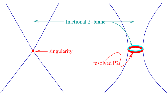
Figure 1: A schematic description of the fractional two-branes both before and after the singularity is resolved.

Consider a two-brane wrapping a non-compact two-cycle. What is the the representation for such branes? In particular, what is its D-brane charge as given by some appropriate Chern character?

In the case of non-compact manifolds the correct framework in which to discuss D-brane charges is compact cohomology or equivalently relative cohomology. For a non-compact manifold $M$ with boundary $N$, the two-brane charges take values in $H^{2}_{\textrm{compact}}(M,\mathbb{Z})\sim H^{2}(M,N,\mathbb{Z})$. A calculation (given in the appendix C.1) shows that this is $\mathbb{Z}$ and since $M$ has only one compact cycle, i.e., the $\mathbb{P}^{2}$, the basic two-brane is obtained by wrapping a $\mathbb{P}^{1}\in\mathbb{P}^{2}$. Hence, $J$ generates $H^{2}(M,N,\mathbb{Z})$. However objects that wrap the non-compact two-cycle of $M$ will have a charge in $H^{2}(M,\mathbb{Z})\sim\mathbb{Z}$. The two cohomologies are related by a long exact sequence, the relevant part of which for our case reduces to the following (see the appendix C.1 for details)

$$0\rightarrow H^{2}({\cal O}_{\mathbb{P}^{2}}(-3),S^{5}/\mathbb{Z}_{3};\mathbb{Z})\rightarrow H^{2}({\cal O}_{\mathbb{P}^{2}}(-3);\mathbb{Z})\stackrel{{\scriptstyle j}}{{\rightarrow}}H^{2}(S^{5}/\mathbb{Z}_{3};\mathbb{Z})\rightarrow 0$$

$$0\rightarrow\mathbb{Z}\stackrel{{\scriptstyle 3}}{{\rightarrow}}\mathbb{Z}\rightarrow\mathbb{Z}_{3}\rightarrow 0$$ (4.17)

Let $J^{\prime}$ generate $H^{2}({\cal O}_{\mathbb{P}^{2}}(-3);\mathbb{Z})$. The exact sequence above indicates that $[J]\sim 3[J^{\prime}]$. Thus if $[J]$ is the charge basis of the 2-brane in the compact cohomology, then a charge $+1$ 2-brane in the compact cohomology would correspond to a charge $+3$ 2-brane in the $[J^{\prime}]$ basis. A single 2-brane wrapping the non-compact two-cycle would have charge $+1$ in the $[J^{\prime}]$ basis or charge $1/3$ in the $[J]$ basis. Thus three two-branes wrapping a non-compact two-cycle of $M$ can give you an object which is equivalent to a two-brane in $\mathbb{P}^{2}$ as elements of $H^{2}({\cal O}_{\mathbb{P}^{2}}(-3),S^{5}/\mathbb{Z}_{3};\mathbb{Z})$. In many ways, this is like the fractional zero-branes – the fractional zero-branes were localised at the singularity and couldn’t be moved away from there unless three of them were taken to form a regular zero-brane.

Thus we have motivated the existence of objects with fractional two-brane charge measured in the charge basis associated with the compact cohomology. We can also perform an equivalent computation in the context of K-theory rather than cohomology, showing again the existence of fractional two-brane charges, but now obviously in the compact K-group associated with the $\mathbb{P}^{2}$. This computation not being essential at this point, is relegated to an appendixC.2.

We can now write down the form of the Chern character for such a fractional two-brane. Clearly its leading term must be of the for $J/3$, while the $J^{2}$ term may depend on whether we have twisted the object by a line bundle ${\cal O}(n)$. Thus the general form will be

$$\textrm{ch}({\cal X}_{m}) = \frac{1}{3}\textrm{ch}[{\cal O}_{\mathbb{P}^{2}}(m-1)\rightarrow{\cal O}_{\mathbb{P}^{2}}(m)]$$ (4.18)

$$= \frac{1}{3}\Big{(}J+\frac{(2m-1)}{2}J^{2}\Big{)}$$

where by construction, ${\cal X}_{m}$ carries $1/3$ the charge of a two-brane on $\mathbb{P}^{2}$ after including a twist which we indicate by the subscript $m$. Note that ${\cal X}_{m+1}={\cal X}_{m}\otimes{\cal O}_{\mathbb{P}^{2}}(1)$ and that $\textrm{ch}({\cal X}_{m+1})=\textrm{ch}({\cal X}_{m})+\frac{1}{3}\ \textrm{ch}({\cal O}_{\rm pt})$.

4.5.2 Fractional two-branes for $\mathbb{C}^{3}/\mathbb{Z}_{3}$

Let us consider the case of fractional two-branes in the $\mathbb{C}^{3}/\mathbb{Z}_{3}$ example. Let us impose Neumann boundary conditions on $(\phi_{1}-\phi_{2})$ and Dirichlet on $(\phi_{1}+\phi_{2})$ and $\phi_{3}$ . Away from the orbifold point, thus there are two fermions (after eliminating $\bar{\xi}_{2}$ in favour of $\bar{\xi}_{1}$): $\bar{\xi}_{1}$ and $\bar{\xi}_{3}$. The gaugino constraint is

$$(\phi_{1}+\phi_{2})\bar{\xi}_{1}+\phi_{3}\bar{\xi}_{3}=0\ .$$ (4.19)

Thus, when $(\phi_{1}+\phi_{2},\phi_{3})\neq(0,0)$, the constraint removes one fermion and when $(\phi_{1}+\phi_{2},\phi_{3})=(0,0)$ the constraint is trivially satisfied. (This is possible, when $\phi_{1}-\phi_{2}\neq 0$.) Repeating the arguments for $\mathbb{C}^{5}/\mathbb{Z}_{5}$, we get three fractional two-branes given by the sequences

$$0\rightarrow F_{0}\rightarrow{\cal O}_{\mathbb{P}^{2}}\rightarrow{\cal X}_{n-1}\otimes{\cal O}_{\mathbb{P}^{2}}(1)\rightarrow 0$$ (4.20)

$$0\rightarrow F_{1}\rightarrow{\cal O}_{\mathbb{P}^{2}}^{\oplus 2}\rightarrow F_{0}\otimes{\cal O}_{\mathbb{P}^{2}}(1)\rightarrow 0$$ (4.21)

$$0\rightarrow F_{2}\rightarrow{\cal O}_{\mathbb{P}^{2}}\rightarrow F_{1}\otimes{\cal O}_{\mathbb{P}^{2}}(1)\rightarrow 0$$ (4.22)

In the first line, we have included the fractional contribution by inserting ${\cal X}_{n-1}$ in the first line of the above equation to complete the sequence.

We then obtain the following identifications

$$\textrm{ch}(F_{0}) = \textrm{ch}\big{[}{\cal O}_{\mathbb{P}^{2}}\big{]}-\textrm{ch}({\cal X}_{n-1})$$ (4.23)

$$-\textrm{ch}(F_{1}) = \textrm{ch}\big{[}{\cal O}_{\mathbb{P}^{2}}(1)-{\cal O}_{\mathbb{P}^{2}}^{\oplus 2}\big{]}-\textrm{ch}({\cal X}_{n})$$ (4.24)

$$\textrm{ch}(F_{2}) = \textrm{ch}\big{[}{\cal O}_{\mathbb{P}^{2}}-{\cal O}_{\mathbb{P}^{2}}^{\oplus 2}(1)+{\cal O}_{\mathbb{P}^{2}}(2)\big{]}-\textrm{ch}({\cal X}_{n+1})$$ (4.25)

The objects in the square brackets are non-fractional objects and hence correspond to coherent sheaves on $\mathbb{P}^{2}$. Thus these terms must necessarily arise from the twisted sectors of the boundary state. The contribution of the untwisted sector is contained in the term containing the ${\cal X}$’s.

Now the Chern character add up as follows:

$$\textrm{ch}(F_{0}-F_{1}+F_{2})=\textrm{ch}\big{[}{\cal O}(2)-{\cal O}(1)\big{]}-J+\frac{(2n+1)}{2}J^{2}$$

where we have kept the two contributions separate. Note that the ${\cal X}$’s have summed up to give an object that has the Chern class of a two-brane on $\mathbb{P}^{2}$.

The Euler form associated with these fractional two-branes, $F_{i}$ have been computed in the appendix B and are generically fractional. However, the intersection form which is obtained by antisymmetrisation of the Euler form is integral[5]. The integrality of the intersection form implies that the charge quantisation condition is not violated. After restricting these sheaves to the Fermat cubic hypersurface in $\mathbb{P}^{2}$, the Euler form reduces to the same intersection matrix without any need for antisymmetrisation. Finally, up to trivial shifts, the intersection matrices also agree with the open-string Witten index computed at the orbifold end. This provides further evidence towards the identification of the $(-)^{I}F_{I}$ as the analytic continuation of the fractional two-branes $S^{(2)}_{I}$ that we constructed at the orbifold end.

A more precise mathematical statement is to write the $F_{i}$ as sheafs in the total space. Let $i$ be the inclusion of the $\mathbb{P}^{2}$ in the total space ${\cal O}_{\mathbb{P}^{2}}(-3)$ and $i_{*}[E]$ represent the push-forward of the bundle $E$ on $\mathbb{P}^{2}$ to the space ${\cal O}_{\mathbb{P}^{2}}(-3)$

$$F_{0} \sim i_{*}\big{[}{\cal O}_{\mathbb{P}^{2}}\big{]}-{\cal X}_{n-1}$$ (4.26)

$$F_{1} \sim i_{*}\big{[}{\cal O}_{\mathbb{P}^{2}}^{\oplus 2}\rightarrow{\cal O}_{\mathbb{P}^{2}}(1)\big{]}-{\cal X}_{n}$$ (4.27)

$$F_{2} \sim i_{*}\big{[}{\cal O}_{\mathbb{P}^{2}}\rightarrow{\cal O}_{\mathbb{P}^{2}}^{\oplus 2}(1)\rightarrow{\cal O}_{\mathbb{P}^{2}}(2)\big{]}-{\cal X}_{n+1}$$ (4.28)

Chern classes on the non-compact space can include terms associated with non-compact divisors. In particular, a term such as $D_{1}\cdot D_{2}$ can appear. Indeed, one has $\textrm{ch}({\cal X}_{n})=D_{1}\cdot D_{2}+\cdots$, where $D_{1}$(resp. $D_{2}$) is the divisor associated to $\phi_{1}=0$ (resp. $\phi_{2}=0$) and the ellipsis contains terms associated with the Chern class of a point. Note that there is nothing fractional about ${\cal X}_{n}$ here. The intersection numbers for the above sheafs can be computed directly in the non-compact space and it reproduces the expected results, without any intervening fractions in the computation. The details of this computation will be presented in [38].

5 The quantum McKay correspondence

It is useful to review some aspects of the McKay correspondence that are relevant for our considerations. Consider the orbifold $\mathbb{C}^{n}/\Gamma$ and its resolution $X$. For the most part, we will be interested in the cases when $\Gamma$ is abelian. It is a correspondence between fractional zero-branes on the orbifold $\mathbb{C}^{n}/\Gamma$, $S_{a}$ ($a$ runs over the irreps of $\Gamma$) and tautological bundles associated with $2n$-branes, $R^{a}$. The $R^{a}$ extend over all of $\mathbb{C}^{n}/\Gamma$ though we usually restrict them to the singularity (or the exceptional divisor(s) when the singularity is resolved). The $S_{a}$ furnish a basis for $K_{c}(X)$, the K-theory classes with compact support on the exceptional divisor(s).

5.1 Review of $\mathbb{C}^{2}/\mathbb{Z}_{n(k)}$

This subsection is based on [22]. Consider the following orbifold action on $\mathbb{C}^{2}$ (with coordinates $(\phi_{1},\phi_{2})$):

$$(\phi_{1},\phi_{2})\rightarrow(\omega\phi_{1},\omega^{k}\phi_{2})$$ (5.1)

where $\omega=\exp(2\pi i/n)$. The case when $k=(n-1)$ is a supersymmetric orbifold and the orbifold is uniquely resolved by blowing up $(n-1)$ $\mathbb{P}^{1}$’s whose intersection matrix is $-1$ times the $A_{n-1}$ Cartan matrix. For general non-supersymmetric $\mathbb{C}^{2}/\mathbb{Z}_{n(k)}$, there is a minimal resolution known as the Hirzebruch-Jung resolution. The resolution consists of $r$ $\mathbb{P}^{1}$’s, where $r$ is the number of terms in the continued fraction expansion of $n/k$:

$$\frac{n}{k}=a_{1}-\frac{1}{a_{2}-\frac{1}{a_{3}-\frac{1}{\cdots 1/a_{r}}}}\equiv[a_{1},a_{2},\ldots,a_{r}]$$ (5.2)

where $a_{\alpha}\geq 2$. There are other resolutions with more $\mathbb{P}^{1}$’s for which some of the $a_{\alpha}=1$. The supersymmetric case occurs when there all the $a_{\alpha}=2$. One can check that $n/(n-1)=[2^{n-1}]$, $3/1=[3]$ and $5/3=[2,3]$ are minimal. The intersection matrix of the $\mathbb{P}^{1}$’s is given by the generalised Cartan matrix

$$C=\begin{pmatrix}a_{1}&-1&0&\cdots&0\\ -1&a_{2}&-1&\cdots&0\\ 0&-1&a_{3}&\ddots&0\\ \vdots&\vdots&\ddots&\ddots&\vdots\\ 0&\cdots&\cdots&&a_{r}\end{pmatrix}$$ (5.3)

5.2 Fractional zero-branes on $\mathbb{C}^{2}/\mathbb{Z}_{n(k)}$

One can construct boundary states for zero-branes on the $\mathbb{C}^{2}/\mathbb{Z}_{n(k)}$ orbifold. Standard methods (analogous to our earlier discussion) lead to $n$ boundary states which we will call fractional zero-branes and label them $S^{\textrm{ns}}_{I}$, $I=1,2,\ldots,n$ where the superscript stands for non-supersymmetric even though there are situations where we have a supersymmetric orbifold. The zero-brane which can move off the orbifold singularity is given by $\sum_{I}S^{\textrm{ns}}_{I}$,

These provide a basis for equivariant K-theory of the orbifold:

$$K_{\mathbb{Z}_{n}}(\mathbb{C}^{2})=\mathbb{Z}\oplus\mathbb{Z}^{n-1}$$ (5.4)

where $\mathbb{Z}$ denotes the non-fractional zero-brane that can move off the singularity and $\mathbb{Z}^{n-1}$, the $(n-1)$ fractional branes that cannot move off the singularity.

5.3 The supersymmetric case: the McKay correspondence

Figure 2: The McKay correspondence for $\mathbb{C}^{n}/\mathbb{Z}_{N}$

The McKay correspondence arises when one considers a resolution $X$ of the orbifold singularity $\mathbb{C}^{2}/\mathbb{Z}_{n(n-1)}$ – for the supersymmetric case, we consider the unique crepant (Calabi-Yau) resolution and for the non-supersymmetric case, we mean the Hirzebruch-Jung resolution. One would like to know the precise objects, i.e., coherent sheaves that correspond to the continuation to large volume of the fractional zero-branes that we obtain at the orbifold point. We will focus on the cases where there is a description of the resolution via the GLSM or equivalently, that the resolved space admits a toric description.

The GLSM for the resolved orbifold will be given by considering $(2+r)$ chiral superfields and $r$ abelian vector multiplets[22], where $r$ is the number of terms in the continued fraction representation of the Hirzebruch-Jung resolution. The orbifold limit is a special point in the Kähler moduli space. Another point of interest is the large-volume point, which corresponds to the point in the moduli space where all the $\mathbb{P}^{1}$’s that appear in the resolution have been blown-up to large sizes. Let $D_{\alpha}$ ($\alpha=1,\ldots,r$) represent the divisors associated with the $r$ $\mathbb{P}^{1}$’s.

In the supersymmetric case which happens when $r=(n-1)$, $R^{I}_{\textrm{ns}}$ turn out to be simple. $(n-1)$ of them are given by the line-bundles ${\cal O}(D_{\alpha})$ and the last one is the trivial line-bundle ${\cal O}_{X}$. These line bundles are called the tautological bundles and provide a basis for $K(X)$, the Grothendieck group of coherent sheaves on $X$ (which is a non-compact CY two-fold).

The fractional zero-branes furnish a basis for the equivariant K-group for the orbifold, i.e., $K_{\mathbb{Z}_{n}}(\mathbb{C}^{2})$. In a similar fashion, it turns out that the the large-volume analogs of the fractional zero-branes $S_{I}^{\textrm{ns}}$ provide a basis for $K^{c}(X)$, the K-theory group with compact support. One expects the isomorphism

$$K_{\mathbb{Z}_{n}}(\mathbb{C}^{2})\sim K^{c}(X)\ .$$

Further, there exists an isomorphism between $K^{c}(X)$ and $K(X)$.

5.4 The non-supersymmetric case: the quantum McKay Correspondence

Martinec and Moore[22] considered the case of non-supersymmetric orbifolds and attempted to find the large-volume analogs of the $R^{I}_{\textrm{ns}}$ here. The natural candidates are the line-bundles ${\cal O}(D_{\alpha})$ and the last one is the trivial line-bundle ${\cal O}_{X}$. There are $(r+1)$ of them as in the supersymmetric case with the only problem being that $r+1<n$. So there are not enough line-bundles to complete the $n$ $R^{I}_{\textrm{ns}}$ at large-volume. The $r+1$ line-bundles are in one-to-one correspondence with the so-called special representations of $\mathbb{Z}_{n}$ in the mathematics literature[34].

We now review the resolution of this puzzle as given in [22]. We will propose another means of resolving this puzzle in the next subsection. The framework used in the GLSM that we discussed earlier where the Hirzebruch-Jung resolution appears in the Higgs branch of the GLSM. It is important to note that the Hirzebruch-Jung resolution is not a crepant one, since $c_{1}(X)<0$. In the quantum GLSM, the world-sheet FI parameters flow under the worldsheet renormalisation group[25]. The singularities are resolved in the IR.

The resolution proposed in [22] is that one must include branes from all quantum vacua. In the IR, the theory has two branches – the Higgs and the Coulomb branches. The missing branes were identified with branes that appeared in the Coulomb branch and were dubbed the Coulomb branch branes. In analogous fashion, the tautological bundles in the Hirzebruch-Jung resolution were called the Higgs branch branes. Further aspects were discussed in a subsequent paper[35] (see also [36, 37]).

5.5 A different interpretation

Figure 3: The proposed quantum McKay correspondence for $\mathbb{C}^{n}/\mathbb{Z}_{N}$

We now consider a different resolution to the puzzle discussed in the previous subsection. Our idea is to embed the non-supersymmetric $\mathbb{C}^{2}/\mathbb{Z}_{n(k)}$ orbifold into a supersymmetric orbifold in one higher dimension, i.e., $\mathbb{C}^{3}/\mathbb{Z}_{n(k)}$, where we have added a third coordinate, lets call it $\phi_{3}$ with the following $\mathbb{Z}_{n}$ action:

$$\phi_{3}\rightarrow\omega^{l}\ \phi_{3},\ \textrm{ where }(l+k+1)=0\textrm{ mod }2n\ .$$ (5.5)

Next, we consider following fractional two-branes on $\mathbb{C}^{3}/\mathbb{Z}_{n}$: Impose Neumann boundary conditions on $\phi_{3}$ and Dirichlet boundary conditions $\phi_{1}=\phi_{2}=0$ on $\phi_{1}$ and $\phi_{2}$. There will be $n$ such fractional two-branes and we will label them $S^{(2)}_{I}$.

Let $\widehat{X}$ be the crepant resolution of $\mathbb{C}^{3}/\mathbb{Z}_{n(k)}$. It is clear that the the projection $\pi:\widehat{X}\rightarrow X$ is obtained by setting $\phi_{3}=0$. As discussed in the previous section, there is a problem similar to the one seen with the non-supersymmetric – the labels $I$ corresponding to the special representations can be obtained using generalisations of the Euler sequences for the fractional zero-branes. In fact, one obtains the following when one restricts the $S^{(2)}_{I}$ to $X$:

$$S^{(2)}_{I}\big{|}_{X}=\left\{\begin{array}[]{ll}S^{\textrm{ns}}_{I}&\textrm{when $I$ corresponds to special representations}\\ 0&\textrm{otherwise}\end{array}\right.\ .$$ (5.6)

This is consistent with our observation in the $\mathbb{C}^{3}/\mathbb{Z}_{3}$ example where branes which disappeared on restriction are those with support on the complex line given by $\phi_{3}\neq 0$ and $\phi_{1}=\phi_{2}=0$. Thus, the field $\phi_{3}$ behaves like an order parameter with $\phi_{3}=0$ corresponding to the Higgs branch branes and $\phi_{3}\neq 0$ giving rise to the Coulomb branch branes of [22].

5.5.1 An example – $\mathbb{C}^{2}/\mathbb{Z}_{3(1)}$

We have already worked out the large volume continuation of the fractional two-branes on $\widehat{X}$. In appendix B, we have provided the Chern classes for these objects. We identified $S^{(2)}_{3}$ as the Coulomb branch brane. What are the candidates for the $R_{(2)}^{I}$’s? In $\widehat{X}$, the $\mathbb{P}^{1}\in\mathbb{P}^{2}$ given by $\phi_{3}=0$ is to be identified with the $\mathbb{P}^{1}$ that appears in the Hirzebruch-Jung resolution $X$ of $\mathbb{C}^{2}/\mathbb{Z}_{3(1)}$. The $R_{\textrm{ns}}^{I}$ corresponding to special representations are ${\cal O}_{X}(-1)$ and ${\cal O}_{X}$. They are “dual” to $S^{(2)}_{1}\big{|}_{X}$ and $S^{(2)}_{2}\big{|}_{X}$. The natural objects on $\widehat{X}$ are the push-forward of the $R$’s on $\mathbb{C}^{2}/\mathbb{Z}_{3(1)}$:

$$R_{(2)}^{1}\sim j_{*}\big{[}{\cal O}_{\widehat{X}}(-1)\big{]}\textrm{ and }R_{(2)}^{2}\sim j_{*}\big{[}{\cal O}_{\widehat{X}}\big{]}$$ (5.7)

where $j$ is the inclusion map from $X$ to $\widehat{X}$. The last object, $R^{(2)}_{3}$ is a little bit more trickier to explain. We do not present the details here – it will be presented in [38]. Its Chern character as well as the those of the above $R_{(2)}^{I}$ can be worked out in the total space using the duality with the $S^{(2)}_{I}$. An important point to emphasise here is that due to the non-compactness of these D-branes, it is better to work in the total space, which is the total space of the line bundle ${\cal O}_{\mathbb{P}^{2}}(-3)$ in our case. In fact, this happens to be true even for fractional zero-branes in cases with several divisors as has been considered in [40, 41].

6 Fractional two-branes and permutation branes

It is of interest to construct the boundary states in the Gepner model associated with linear boundary conditions that we considered in the LG orbifolds. This is what we shall pursue in this section.

6.1 A conjecture

Consider the holomorphic involution $\pi$ that permutes two fields :

$$\pi:\quad\phi_{1}\leftrightarrow\phi_{2}$$

The fixed point(s) of the action is $\phi_{1}+\phi_{2}=0,\phi_{3}=\phi_{4}=\phi_{5}=0$ (this is a two-brane which we called $P$ which restricts to a point on the quintic $Q$) as well as $\phi_{1}-\phi_{2}=0$(this is an eight-brane which restricts to a four-brane on the quintic). Thus, we see the appearance of the boundary conditions of Eq. (2.5) as one of the fixed point sets of the holomorphic involution. This suggests that the permutation branes of ref. [23], in particular, those corresponding to $\pi=(12)(3)(4)(5)$ may be the correct candidate for the boundary states in the Gepner model that correspond to the boundary conditions given in Eq. (3.5). This leads to the following conjecture:

Conjecture: The B-type permutation branes labelled

$$|0,0,0,0,M,\widetilde{M}\rangle_{\pi}\quad,\ \pi=(12)(3)(4)(5)$$

of ref.[23] are the CFT boundary states for the boundary conditions given in Eq. (2.5) associated with the fractional two-branes.

6.2 Checks of the conjecture

A first check: Recall, that we had obtained five fractional two-branes at large volume in section 3. But, we have $25$ boundary states since both $M$ and $\widetilde{M}$ each take $5$ values. How can this make sense? In this regard it is useful to recall that there is a $(\mathbb{Z}_{5})^{5}$ symmetry in the minimal models as well as their corresponding LG models which act as

$$g_{i}:\quad\phi_{i}\rightarrow\omega\ \phi_{i}\quad,\ g_{i}^{5}=1\ ,$$

where $\omega$ is a non-trivial fifth-root of unity. Focusing on the $(\mathbb{Z}_{5})^{2}$ which act on the fields $\phi_{1}$ and $\phi_{2}$, we see that the boundary condition $(\phi_{1}+\phi_{2})=0$ is invariant only under the simultaneous action $g_{1}g_{2}$ while $g_{1}$ or $g_{2}$ or the combination $g_{1}g_{2}^{-1}$ act as boundary condition changing operators. Thus, the 25 boundary states in the CFT (of [23]) correspond to the five sets of boundary conditions:

$$\phi_{1}+\omega^{a}\phi_{2}=0\quad,\ a=0,1,2,3,4.$$ (6.1)

Thus, the $\widetilde{M}$ index can be identified with $2a$.

A second check: Ref. [23] provides the intersection matrix between the permutation branes (though the normalisation of the boundary states was not fixed in that paper). The result which we quote here (after fixing the normalisation) is the following: the intersection form is independent of $\widetilde{M}$ and is given by $g(1-g)^{3}$. It is easy to see that the fractional two-branes that we propose at large volume also have the same intersection matrix (see appendix A). Since the intersection form does depends on only the Chern character (equivalently, RR charges) of the coherent sheaves, it will necessarily be independent of the $\widetilde{M}$ label. For instance, the D0-branes obtained from the boundary conditions, (6.1), are located at different points on the quintic. However, their charges are identical.

A third check: A last check is to compute the intersection matrix between the $(12)(3)(4)(5)$ permutation boundary states and the RS boundary states and show that it equals $-(1-g)^{4}$ as obtained in the appendix A by computing the intersection matrix between the RS vector bundles and coherent sheaves for the fractional two-branes. This is a little bit more subtle since it involves characters that are not present in the bulk/closed string partition function. This issue has been discussed in a recent paper, so we do not present any details but refer the reader to it for a more detailed discussion[24]. As is finally shown in there, the intersection matrix does take the form $-(1-g)^{4}$ as predicted by the conjecture.

6.3 Other permutation branes

It is natural to see if other permutation branes can be obtained by considering other linear boundary conditions involving more fields. One obvious candidate for the LG boundary conditions associated with the permutation brane $(12)(34)(5)$:

$$\phi_{1}+\phi_{2}=\phi_{3}+\phi_{4}=\phi_{5}=0\ .$$ (6.2)

This will be a fractional four-brane and the open-string Witten index computation in section 4 for fractional four-branes can be compared with the intersection matrices for the $(12)(34)(5)$ branes. The Coulomb branes have support on the hypersurface $S$ corresponding to the conditions given in Eq. (6.2). This intersects the $\mathbb{P}^{4}$ on a $\mathbb{P}^{1}$. The Coulomb branes will be given by ${\cal X}_{S}\otimes{\cal O}(-1)$ and ${\cal X}_{S}\otimes{\cal O}$, where ${\cal X}_{S}$ is the sheaf with support on the hypersurface $S$ (and Chern class $J^{2}/5$ reflecting the fractional charge) and $({\cal O},{\cal O}(1))$ are the tautological bundles on $\mathbb{P}^{1}$. Thus, their Chern classes will be

$$\frac{J^{2}}{5}-\frac{J^{3}}{5}\ ,\textrm{ and }\frac{J^{2}}{5}\ .$$

This is consistent with the Chern classes of the permutation branes labelled $V_{3}$ and $V_{4}$ in Eq. (6.13) of [24]. These restrict to a two-brane (of minimal charge) on the quintic. The Higgs branes will be related to Euler sequences on $\mathbb{P}^{2}$. The other branes given in the aforementioned reference also seem to fit this. So this also passes a similar set of checks. Thus, for the quintic, one is able to obtain objects which reproduce the full spectrum of charges – the fractional two-branes providing the zero-brane and the fractional four-brane providing the two-brane.

Another interesting boundary condition in the LG orbifold is the fractional four-brane given by

$$\phi_{1}+\phi_{2}+\phi_{3}=\phi_{4}=\phi_{5}=0\ .$$

This involves three fields and seems to be related to the permutation brane $(123)(4)(5)$. However, this runs into trouble in the first check correspond to . The permutation branes constructed in [23] do not have enough labels to account for the $125$ boundary states that one anticipates by considering the action of the symmetries on this boundary condition. In this regard, we wish to point out that for cyclic orbifolds[42, 43], $\mathbb{Z}_{\lambda}$ with $\lambda>2$, there is a fixed point resolution problem, related to the fact that the different primaries in the orbifold theory have the same character (see section 5 of [43]). This also suggests that the set of permutation branes given in [23] may not be minimal and their resolution will provide us with additional boundary states that may account for the $125$ boundary states that we predict. We hope to discuss this issue in a future publication.

7 Conclusion and Summary

We first summarise the main results of this paper.

• We have provided evidence that the new fractional branes obtained in [13] using the method of matrix factorisation and boundary fermions are the same as those given by the boundary conditions proposed in [2]. The methods used in this paper also lead to sequences for the new fractional branes which carry more information than Chern classes/RR charges. As a consequence, we show that fractional $2p$-branes constructed in the non-compact Calabi-Yau restrict to the compact Calabi-Yau hypersurface as well defined objects.

• We also provided evidence that a sub-class of the permutation branes proposed in [23] are related to the new fractional branes. This result has also been independently obtained by Brunner and Gaberdiel recently[24]. In particular, a detailed discussion of the permutation branes and the intersection matrices amongst them has been provided in their paper.

• By embedding non-supersymmetric orbifolds into supersymmetric orbifolds in one higher dimension, we propose a quantum McKay correspondence that relates fractional $2p$-branes on $\mathbb{C}^{n}/\mathbb{Z}_{N}$ to (the push-forward of) tautological bundles on $\mathbb{C}^{n-p}/\mathbb{Z}_{N}$ branes in supersymmetric orbifolds. We also provide an alternate explanation to the “missing” branes discussed in [22].

This paper has dealt with, in many ways, the easiest of the examples. Possible generalisations include the consideration of other examples involving weighted projective spaces – these typically involve many Kähler moduli and the sequences that we proposed in this paper for the new fractional branes will have a more complicated realisation. We plan to discuss this in [38].

Another class of boundary conditions that can appear in these examples are those that are not linear. For instance, consider the boundary condition $(\phi_{1}+\phi_{2}^{2})=0$ that is consistent with the $G=0$ condition. How does one construct the boundary states corresponding to such a boundary condition? An added complication is that they do not seem to be minimal submanifolds. What are their intersection forms? In fact, it has been argued in [24] that in more complicated examples, the addition of the analogue of the fractional two-branes and four-branes that we have considered do not give rise to all possible RR charge vectors. Thus, one may be forced to deal with such boundary conditions. However the Gepner model for such examples typically involve minimal models with even level $k$. Here, even the RS boundary states are not minimal in the Cardy sense. So the issue is somewhat clouded by the need to resolve the boundary states.

Coming back to the case of the quintic – while it is indeed satisfying to find objects in the Gepner model/LG orbifold which provide all RR charges that appear on the quintic, it cannot be the end of the story. The RS boundary states were related to spherical objects (spherical in the sense that these objects have only ${\rm Hom}(E,E)\equiv{\rm Ext}^{3}(E,E)\neq 0$) on the quintic even though they did not span the lattice of RR charges. One would like to know, if there exists a basis of, say, four spherical objects on the quintic that give rise to all possible charges via bound state formation. In the framework of boundary fermions and matrix factorisation the superpotentials on these branes have been computed and their relationship to obstruction theory has been discussed. It would be interesting to see if those computations agree with an extension of the superpotential computation carried out for the RS branes in the LG model in[44] to the case of the fractional two-branes and four-branes.

In this paper, we have shown a parallel between fractional $2p$-branes on supersymmetric orbifolds and fractional zero-branes on non-supersymmetric orbifolds of dimensional lower by one. The Coulomb branes in the non-supersymmetric orbifolds have been identified with the minima of the quantum superpotential of twisted chiral superfields. The Coulomb branes, as we refer to them, among the fractional two-branes in our construction are associated with a chiral superfield. It appears possible to make the connection between the two situations precise by applying the Hori-Vafa map[45], which relates chiral superfields to twisted chiral superfields. This issue as well as an explanation for the change of basis proposed in [35] will be discussed in [39].

Our reinterpretation of the quantum McKay correspondence will be useful for non-supersymmetric orbifolds in higher dimensions such as $\mathbb{C}^{3}/\mathbb{Z}_{n}$ [36, 37] where there is no analogue of the Hirzebruch-Jung resolution via partial fractions. There is also the problem of terminal singularities that can appear. At least in cases where the higher dimensional supersymmetric orbifold admits a crepant resolution, one will be able to use the embedding to study aspects of the non-supersymmetric orbifold such as the possible end-points of tachyon condensation.

Acknowledgments: We thank A. Adams, Shiraz Minwalla, Kapil Paranjape, K. Ray, T. Sarkar and T. Takayanagi for useful conversations. S.G. would like to thank Shiraz Minwalla and the Physics Department of Harvard University for hospitality where some of this work was done during summer 2004. T.J would like to thank the Dept. of Theoretical Physics, TIFR for hospitality where part of this work was done. B.E. would like to thank Dept. of Theoretical Physics, TIFR for hospitality during the summer of 2004. T.J. would like to thank N. Nitsure and V. Srinivas for several explanations and useful discussions that were important to understanding the mathematics relevant to this paper.

Appendix A Intersection matrices for the quintic

The Chern character of the RS branes on the Fermat quintic $Q\in\mathbb{P}^{4}$ are obtained from the generalised Euler sequences given in Eq. (3.3). One obtains

$$\textrm{ch}({\cal M}_{0}) = 1$$

$$\textrm{ch}({\cal M}_{1}) = -4+J+\frac{J^{2}}{2}+\frac{J^{3}}{6}$$

$$\textrm{ch}({\cal M}_{2}) = 6-3\,J-\frac{J^{2}}{2}+\frac{J^{3}}{2}$$

$$\textrm{ch}({\cal M}_{3}) = -4+3\,J-\frac{J^{2}}{2}-\frac{J^{3}}{2}$$

$$\textrm{ch}({\cal M}_{4}) = 1-J+\frac{J^{2}}{2}-\frac{J^{3}}{6}$$

In the above $J$ generates $H^{2}(Q,\mathbb{R})$ with the normalisation chosen to be $\langle J^{3}\rangle_{Q}=5\langle J^{4}\rangle_{\mathbb{P}^{4}}=5$. The Chern character for the new fractional branes are given in terms of the sequences that we proposed in Eqs. (3.8). The only additional input is our proposal that $\textrm{ch}({\cal X}_{P})=\frac{J^{3}}{5}$.

$$\textrm{ch}({\cal F}_{0}) = 1-\frac{J^{3}}{5}$$

$$\textrm{ch}({\cal F}_{1}) = -3+J+\frac{J^{2}}{2}-\frac{J^{3}}{30}$$

$$\textrm{ch}({\cal F}_{2}) = 3-2\,J+\frac{7\,J^{3}}{15}$$

$$\textrm{ch}({\cal F}_{3}) = -1+J-\frac{J^{2}}{2}-\frac{J^{3}}{30}$$

$$\textrm{ch}({\cal F}_{4}) = \frac{-J^{3}}{5}$$

The Euler form on the quintic is defined as

$$\chi(E,F)=\int_{Q}\textrm{ch}(E)^{*}\ \textrm{ch}(F)\ \textrm{Td}(Q)\ ,$$

A standard computation (easily done using symbolic manipulation programs) using the above formula leads to the following intersection matrices are:

$$\chi({\cal M}_{\mu},{\cal M}_{\nu})=\begin{pmatrix}0&5&-10&10&-5\\ -5&0&5&-10&10\\ 10&-5&0&5&-10\\ -10&10&-5&0&5\\ 5&-10&10&-5&0\end{pmatrix}\longleftrightarrow-(1-g)^{5}$$ (A.1)

$$\chi({\cal M}_{\mu},{\cal F}_{\nu})=\begin{pmatrix}-1&4&-6&4&-1\\ -1&-1&4&-6&4\\ 4&-1&-1&4&-6\\ -6&4&-1&-1&4\\ 4&-6&4&-1&-1\end{pmatrix}\longleftrightarrow-(1-g)^{4}$$ (A.2)

$$\chi({\cal F}_{\mu},{\cal F}_{\nu})=\begin{pmatrix}0&1&-3&3&-1\\ -1&0&1&-3&3\\ 3&-1&0&1&-3\\ -3&3&-1&0&1\\ 1&-3&3&-1&0\end{pmatrix}\longleftrightarrow g(1-g)^{3}$$ (A.3)

where we have rewritten the matrices in terms of the generator $g$ of the quantum $\mathbb{Z}_{5}$ symmetry. The last formula coincides with the intersection matrix computed between the $L=0$ permutation branes for $\pi=(12)345$ given in the appendix of [23].

Appendix B Intersection matrices for $\mathbb{C}^{3}/\mathbb{Z}_{3}$

In this appendix, we present the computation of various intersection matrices for the coherent sheaves given by the sequences written out for fractional zero and two-branes. We present the Chern classes after restriction to the $\mathbb{P}^{2}$. The Chern classes for the fractional zero-branes are given from the Euler sequences for $\mathbb{P}^{2}$

$$S^{(0)}_{1} = 1$$ (B.1)

$$S^{(0)}_{2} = -2+J+\frac{J^{2}}{2}$$ (B.2)

$$S^{(0)}_{3} = 1-J+\frac{J^{2}}{2}$$ (B.3)

The Chern classes for the fractional two-branes are

$$S^{(2)}_{1} = 1-\frac{J}{3}-\frac{(2m+3)J^{2}}{6}$$ (B.4)

$$S^{(2)}_{2} = -1+\frac{2\,J}{3}-\frac{(m+1)J^{2}}{3}$$ (B.5)

$$S^{(2)}_{3} = -\frac{J}{3}-\frac{(2m+1)J^{2}}{6}$$ (B.6)

The various Euler forms given below are obtained using the formula:

$$\chi(E,F)=\int_{\mathbb{P}^{2}}\textrm{ch}(E)^{*}\ \textrm{ch}(F)\ \textrm{Td}(\mathbb{P}^{2})\$$

$$\chi(S^{(0)},S^{(0)})=\begin{pmatrix}1&0&0\\ -3&1&0\\ 3&-3&1\end{pmatrix}$$ (B.7)

$$\chi(S^{(2)},S^{(0)})=\frac{1}{3}\begin{pmatrix}-m+3&2m+1&-m-1\\ -m-7&2m+6&-m-2\\ -m+1&2m-1&-m\end{pmatrix}$$ (B.8)

$$\chi(S^{(0)},S^{(2)})=\frac{1}{3}\begin{pmatrix}-m&-1-m&-m-2\\ 2m-2&2m+3&2m+5\\ -m+5&-m-5&-m-3\end{pmatrix}$$ (B.9)

$$\chi(S^{(2)},S^{(2)})=\frac{1}{9}\begin{pmatrix}-6m-1&-1&-3m-7\\ -10&6m+11&3m+8\\ -3m+2&3m-1&-1\end{pmatrix}$$ (B.10)

For bundles on a Calabi-Yau manifold these are antisymmetric. However, for bundles on divisors or more generally sheaves, the intersection form is obtained by explicitly antisymmetrising the above(as explained in [5]), i.e., let

$$I(E^{\prime},E)\equiv\chi(E^{\prime},E)-\chi(E,E^{\prime})$$

for any two sheaves $E$ and $E^{\prime}$. In our case, we then get

$${\cal I}^{0,0}\equiv I(S^{(0)},S^{(0)}) = -(1-g)^{3}$$

$${\cal I}^{0,2}\equiv I(S^{(0)},S^{(2)}) = -(1-g)^{2}$$ (B.11)

$${\cal I}^{2,2}\equiv I(S^{(2)},S^{(2)}) = g(1-g)$$

Note that the dependence on $m$ disappears in the intersection matrix and thus we cannot fix its value. However, this is to be expected since a change in $m$ is obtained by twisting by ${\cal O}(1)$, which is the monodromy at large volume. Since these sheaves are obtained via analytic continuation, the ambiguity in $m$ is related to the possibility of choosing paths from the orbifold point to large volume which differ by a path around the large-volume point. The fact that the above matrix has integer entries implies that the DSZ charge quantisation condition is satisfied. Thus it is correct to assume that the fractional two-branes do carry fractional two-brane RR charge and not integral as suggested in [31] (in particular see appendix A, Eq. (A31)) suggests.

Appendix C Cohomology and K-theory computations

C.1 Relevant cohomology groups for ${\cal O}_{\mathbb{P}^{2}}(-3)$

We consider a spacetime of the form $\mathbb{R}\times M$, where $\mathbb{R}$ represents the time direction and $M$ is non-compact. Let $N$ be the boundary of $M$. The D-brane charges take values in the relative cohomology $H^{*}(M,N;\mathbb{Z})$[46]. These can be computed by considering the long-exact sequence in cohomology:

$$\cdots\rightarrow H^{p}(M;\mathbb{Z})\stackrel{{\scriptstyle j}}{{\rightarrow}}H^{p}(N;\mathbb{Z})\rightarrow H^{p+1}(M,N;\mathbb{Z})\stackrel{{\scriptstyle i}}{{\rightarrow}}H^{p+1}(M;\mathbb{Z})\rightarrow\cdots$$ (C.1)

The map $j$ corresponds to restricting $p$-forms on $M$ to the boundary $N$. Let us choose $M$ to be $\mathbb{C}^{3}/\mathbb{Z}_{3}$ (or equivalently ${\cal O}_{\mathbb{P}^{2}}(-3)$). Then, one has $N=\partial M=S^{5}/\mathbb{Z}_{3}$. One has the following non-vanishing cohomologies for $N$ and $M$.

$$H^{4}(S^{5}/\mathbb{Z}_{3};\mathbb{Z}) = H^{2}(S^{5}/\mathbb{Z}_{3};\mathbb{Z})=\mathbb{Z}_{3}\quad,$$

$$H^{0}(S^{5}/\mathbb{Z}_{3};\mathbb{Z}) = H^{5}(S^{5}/\mathbb{Z}_{3};\mathbb{Z})=\mathbb{Z}\quad,\quad$$ (C.2)

$$H^{2p}({\cal O}_{\mathbb{P}^{2}}(-3);\mathbb{Z}) = H^{2p}(\mathbb{P}^{2};\mathbb{Z})=\mathbb{Z}\quad,\quad\textrm{for }p=0,1,2\quad,$$

Using the above data, we obtain the long-exact sequence breaks into four shorter sequences:

$$0\rightarrow H^{0}({\cal O}_{\mathbb{P}^{2}}(-3),S^{5}/\mathbb{Z}_{3};\mathbb{Z})\rightarrow\mathbb{Z}\stackrel{{\scriptstyle j}}{{\rightarrow}}\mathbb{Z}\rightarrow H^{1}({\cal O}_{\mathbb{P}^{2}}(-3),S^{5}/\mathbb{Z}_{3};\mathbb{Z})\rightarrow 0$$ (C.3)

$$0\rightarrow H^{2}({\cal O}_{\mathbb{P}^{2}}(-3),S^{5}/\mathbb{Z}_{3};\mathbb{Z})\rightarrow\mathbb{Z}\stackrel{{\scriptstyle j}}{{\rightarrow}}\mathbb{Z}_{3}\rightarrow H^{3}({\cal O}_{\mathbb{P}^{2}}(-3),S^{5}/\mathbb{Z}_{3};\mathbb{Z})\rightarrow 0$$ (C.4)

$$0\rightarrow H^{4}({\cal O}_{\mathbb{P}^{2}}(-3),S^{5}/\mathbb{Z}_{3};\mathbb{Z})\rightarrow\mathbb{Z}\stackrel{{\scriptstyle j}}{{\rightarrow}}\mathbb{Z}_{3}\rightarrow H^{5}({\cal O}_{\mathbb{P}^{2}}(-3),S^{5}/\mathbb{Z}_{3};\mathbb{Z})\rightarrow 0$$ (C.5)

$$0\rightarrow\mathbb{Z}\rightarrow H^{6}({\cal O}_{\mathbb{P}^{2}}(-3),S^{5}/\mathbb{Z}_{3};\mathbb{Z})\rightarrow 0$$ (C.6)

In the first equation above, the map $j$ corresponds to restricting (constant) functions on ${\cal O}_{\mathbb{P}^{2}}(-3)$ to the boundary $S^{5}/\mathbb{Z}_{3}$. Clearly, this is an isomorphism and hence we obtain $H^{0}({\cal O}_{\mathbb{P}^{2}}(-3),S^{5}/\mathbb{Z}_{3};\mathbb{Z})$ and $H^{1}({\cal O}_{\mathbb{P}^{2}}(-3),S^{5}/\mathbb{Z}_{3};\mathbb{Z})$ both vanish. The last equation implies that $H^{6}({\cal O}_{\mathbb{P}^{2}}(-3),S^{5}/\mathbb{Z}_{3};\mathbb{Z})=\mathbb{Z}$. It can be shown that all odd (relative) cohomologies vanish. Thus, the second and third equations above reduce to

$$0\rightarrow H^{2p}({\cal O}_{\mathbb{P}^{2}}(-3),S^{5}/\mathbb{Z}_{3};\mathbb{Z})\stackrel{{\scriptstyle a}}{{\rightarrow}}\mathbb{Z}\stackrel{{\scriptstyle j}}{{\rightarrow}}\mathbb{Z}_{3}\rightarrow 0\quad(\textrm{for }p=1,2)$$

This implies that both above relative cohomologies are $\mathbb{Z}$ with the first map $a$ representing multiplication by $3$. Thus, one has the following result:

$$\boxed{H^{2p}({\cal O}_{\mathbb{P}^{2}}(-3),S^{5}/\mathbb{Z}_{3};\mathbb{Z})=\mathbb{Z}\quad(\textrm{for }p=1,2,3)}$$ (C.7)

C.2 The K-theory computation

The K-theory computation in the relative case of a manifold with boundary that parallels the computation of C.1 may also be carried out. In the case at had we are interested in computing the relative K-groups of the total space of the bundle ${\cal O}(-3)$ on $\mathbb{P}^{2}$ with respect to the boundary $S^{5}/BZ_{3}$. The computation is done by examining, as is typical in such situations, a six-term exact sequence (a consequence of collapsing a long exact sequence of K-groups using Bott periodicity) and using the known results on the K-group of $\mathbb{P}^{2}$ to compute the relative K-groups of interest. A useful reference for the computations of this section is [47].

We will take as the manifold $M$, the disc bundle $D(E)$ related to the bundle $E$ defined by taking all vectors $v$ in $E$ such that their inner product (defined with respect to some appropriate Riemannian metric on $E$) $\langle v,v\rangle\leq 1$. The boundary of $D(E)$ will be sphere bundle $S(E)$ made of vectors $v$ in $E$ such that $\langle v,v\rangle=1$. By a standard argument, the relative K-groups $K(D(E),S(E))$ may be identified with the K-groups $K(E,E_{0})$ where $E_{0}$ is the complement of the zero-section of $E$.

To compute the K-groups $K(M,\partial M)$ for a compact manifold $M$ with boundary $\partial M$ we may use the following six-term exact sequence:

$$K^{0}(M)\rightarrow K^{0}(\partial M)\rightarrow K^{1}(M,\partial M)\rightarrow K^{1}(M)\rightarrow$$ (C.8)

$$\rightarrow K^{1}(\partial M)\rightarrow K^{0}(M,\partial M)\rightarrow K^{0}(M).$$

In our case $M=D(E)$, $\partial M=S(E)$. For the case of the disc bundle since it is a deformation retract of $E$ itself and the K-group of a bundle is isomorphic to the K-group of the base, we have $K(D(E))=K(\mathbb{P}^{2})$. To compute $K(S)$ we may compute it knowing the cohomology of $S(E)=S^{5}/\mathbb{Z}_{3}$. Though strictly speaking we should use the machinery of the Atiyah-Hirzebruch spectral sequence, it appears here to provide no surprises. We therefore get a $K^{0}(S(E))$ and $K^{1}(S(E))$ that is isomorphic to the cohomology.

We may now do the computation, using the data on the K-groups of $S(E)$ and $K(\mathbb{P}^{2})$ (in particular, $K^{1}(\mathbb{P}^{2})=0$, since all the odd cohomologies of $\mathbb{P}^{2}$ are zero) to obtain the following shorter exact sequence:

$$0\rightarrow K^{1}(S^{5}/\mathbb{Z}_{3})\rightarrow K^{0}({\cal O}(-3),S^{5}/\mathbb{Z}_{3})\rightarrow K^{0}(\mathbb{P}^{2})\rightarrow K^{0}(S^{5}/\mathbb{Z}_{3})\rightarrow 0.$$ (C.9)

Using the data

$$K^{0}(\mathbb{P}^{2})=\mathbb{Z}\oplus\mathbb{Z}\oplus\mathbb{Z};K^{0}(S^{5}/\mathbb{Z}_{3})=\mathbb{Z}\oplus\mathbb{Z}_{3}\oplus\mathbb{Z}_{3};K^{1}(S^{5}/\mathbb{Z}_{3})=\mathbb{Z}$$ (C.10)

we obtain the result

$$K^{0}(M,\partial M)=\mathbb{Z}\oplus\mathbb{Z}\oplus\mathbb{Z}$$ (C.11)

Note that one $Z$ is in the kernel of the map from $K^{0}(M,\partial M)$ to $K^{0}(P^{2})$. Two of the $Z$ factors in $K^{0}(M,\partial M)$ form part of the sequence of the type

$$0\rightarrow\mathbb{Z}\stackrel{{\scriptstyle n}}{{\rightarrow}}\mathbb{Z}\rightarrow\mathbb{Z}_{n}\rightarrow 0.$$ (C.12)

where $n=3$ in our case. What this shows is that if $[J^{\prime}]$ is the generator of $K^{0}(P^{2})$ and $[J]$ is the generator of $K^{0}(M,\partial M)$ then $[J]\sim 3[J^{\prime}]$. If we take the standard unit of 2-brane charges to be given by $[J]$, then a $1/3$ charge in the $[J]$ basis becomes an integer charge in the $[J^{\prime}]$ basis.

References

- [1] I. Brunner, M. R. Douglas, A. E. Lawrence and C. Romelsberger, “D-branes on the quintic,” JHEP 0008 (2000) 015 [arXiv:hep-th/9906200].
- [2] S. Govindarajan, T. Jayaraman and T. Sarkar, “Worldsheet approaches to D-branes on supersymmetric cycles,” Nucl. Phys. B 580, 519 (2000) [arXiv:hep-th/9907131].
-
[3]
M. R. Douglas,
“Lectures on D-branes on Calabi-Yau manifolds,”
Lectures at the 2001 ICTP Spring School on Superstrings and Related
Matters, online proceedings are
available at the URL
http://www.ictp.trieste.it/~pub_off/lectures/vol7.html - [4] A. Recknagel and V. Schomerus, “D-branes in Gepner models,” Nucl. Phys. B 531, 185 (1998) [arXiv:hep-th/9712186].
- [5] M. R. Douglas, B. Fiol and C. Römelsberger, “Stability and BPS branes,” hep-th/0002037.
- [6] M. R. Douglas, B. Fiol and C. Romelsberger, “The spectrum of BPS branes on a noncompact Calabi-Yau,” arXiv:hep-th/0003263.
- [7] D. E. Diaconescu and M. R. Douglas, “D-branes on stringy Calabi-Yau manifolds,” arXiv:hep-th/0006224.
- [8] S. Govindarajan and T. Jayaraman, “D-branes, exceptional sheaves and quivers on Calabi-Yau manifolds: From Mukai to McKay,” Nucl. Phys. B 600, 457 (2001) [arXiv:hep-th/0010196].
- [9] A. Tomasiello, “D-branes on Calabi-Yau manifolds and helices,” JHEP 0102, 008 (2001) [arXiv:hep-th/0010217].
- [10] P. Mayr, “Phases of supersymmetric D-branes on Kaehler manifolds and the McKay correspondence,” JHEP 0101 (2001) 018 [arXiv:hep-th/0010223].
- [11] W. Lerche, P. Mayr and J. Walcher, “A new kind of McKay correspondence from non-Abelian gauge theories,” arXiv:hep-th/0103114.
-
[12]
A. Kapustin and Y. Li,
“D-branes in Landau-Ginzburg models and algebraic geometry,”
JHEP 0312, 005 (2003)
[arXiv:hep-th/0210296].
“Topological correlators in Landau-Ginzburg models with boundaries,” Adv. Theor. Math. Phys. 7, 727 (2004) [arXiv:hep-th/0305136].
“D-branes in topological minimal models: The Landau-Ginzburg approach,” JHEP 0407, 045 (2004) [arXiv:hep-th/0306001]. - [13] S. K. Ashok, E. Dell’Aquila and D. E. Diaconescu, “Fractional branes in Landau-Ginzburg orbifolds,” arXiv:hep-th/0401135.
-
[14]
K. Hori and J. Walcher,
“F-term equations near Gepner points,”
JHEP 0501, 008 (2005)
[arXiv:hep-th/0404196].
“D-branes from matrix factorizations,” Comptes Rendus Physique 5, 1061 (2004) [arXiv:hep-th/0409204]. -
[15]
I. Brunner, M. Herbst, W. Lerche and B. Scheuner,
“Landau-Ginzburg realization of open string TFT,”
arXiv:hep-th/0305133.
I. Brunner, M. Herbst, W. Lerche and J. Walcher, “Matrix factorizations and mirror symmetry: The cubic curve,” arXiv:hep-th/0408243. - [16] J. Walcher, “Stability of Landau-Ginzburg branes,” arXiv:hep-th/0412274.
- [17] S. K. Ashok, E. Dell’Aquila, D. E. Diaconescu and B. Florea, “Obstructed D-branes in Landau-Ginzburg orbifolds,” arXiv:hep-th/0404167.
-
[18]
D. Orlov,
“Triangulated categories of singularities and D-branes in
Landau-Ginzburg models,”
arXiv:math.ag/0302304.
“Triangulated categories of singularities and equivalences between Landau-Ginzburg models,” arXiv:math.ag/0503630.
“Derived categories of coherent sheaves and triangulated categories of singularities,” arXiv:math.ag/0503632. - [19] S. Govindarajan and T. Jayaraman, “Boundary fermions, coherent sheaves and D-branes on Calabi-Yau manifolds,” Nucl. Phys. B 618, 50 (2001) [arXiv:hep-th/0104126].
- [20] C. Romelsberger, “(Fractional) intersection numbers, tadpoles and anomalies,” arXiv:hep-th/0111086.
- [21] M. Billo, B. Craps and F. Roose, “Orbifold boundary states from Cardy’s condition,” JHEP 0101 (2001) 038 [arXiv:hep-th/0011060].
- [22] E. J. Martinec and G. W. Moore, “On decay of K-theory,” arXiv:hep-th/0212059.
- [23] A. Recknagel, “Permutation branes,” JHEP 0304 (2003) 041 [arXiv:hep-th/0208119].
- [24] I. Brunner and M. R. Gaberdiel, “Matrix factorisations and permutation branes,” arXiv:hep-th/0503207.
- [25] E. Witten, “Phases of Theories in Two Dimensions,” Nucl. Phys. B403 (1993) 159 [arXiv:hep-th/9301042].
- [26] S. Govindarajan, T. Jayaraman and T. Sarkar, “On D-branes from gauged linear sigma models,” Nucl. Phys. B 593, 155 (2001) [arXiv:hep-th/0007075].
-
[27]
S. Govindarajan and T. Jayaraman,
“On the Landau-Ginzburg description of boundary CFTs and special Lagrangian
submanifolds,”
JHEP 0007 (2000) 016
[arXiv:hep-th/0003242].
K. Hori, A. Iqbal and C. Vafa, “D-branes and mirror symmetry,” arXiv:hep-th/0005247. - [28] I. Brunner and J. Distler, “Torsion D-branes in nongeometrical phases,” Adv. Theor. Math. Phys. 5 (2002) 265 [arXiv:hep-th/0102018].
- [29] D. E. Diaconescu and J. Gomis, “Fractional branes and boundary states in orbifold theories,” JHEP 0010 (2000) 001 [arXiv:hep-th/9906242].
- [30] M. R. Gaberdiel and B. J. Stefanski, “Dirichlet branes on orbifolds,” Nucl. Phys. B 578 (2000) 58 [arXiv:hep-th/9910109].
- [31] T. Takayanagi, “Holomorphic tachyons and fractional D-branes,” Nucl. Phys. B 603 (2001) 259 [arXiv:hep-th/0103021].
-
[32]
M. Bertolini, P. Di Vecchia, M. Frau, A. Lerda, R. Marotta and I.
Pesando,
”Fractional D-branes and their gauge duals”
JHEP 0102 (2001) 014
[arXiv:hep-th/0011077]
M. Bertolini, P. Di Vecchia, M. Frau, A. Lerda and R. Marotta, “N = 2 gauge theories on systems of fractional D3/D7 branes,” Nucl. Phys. B 621 (2002) 157 [arXiv:hep-th/0107057]. - [33] M. R. Gaberdiel and H. Klemm, “N = 2 superconformal boundary states for free bosons and fermions,” Nucl. Phys. B 693 (2004) 281 [arXiv:hep-th/0404062].
- [34] O. Riemenschneider, “Special representations and the two-dimensional McKay correspondence,” Hokkaido Math. Journal XXXII (2003) 317-333.
- [35] G. W. Moore and A. Parnachev, “Localized tachyons and the quantum McKay correspondence,” JHEP 0411 (2004) 086 [arXiv:hep-th/0403016].
- [36] T. Sarkar, “On localized tachyon condensation in and ,” Nucl. Phys. B 700 (2004) 490 [arXiv:hep-th/0407070].
-
[37]
D. R. Morrison, K. Narayan and M. R. Plesser,
“Localized tachyons in ,”
JHEP 0408, 047 (2004)
[arXiv:hep-th/0406039].
D. R. Morrison and K. Narayan, “On tachyons, gauged linear sigma models, and flip transitions,” JHEP 0502, 062 (2005) [arXiv:hep-th/0412337]. - [38] Bobby Ezhuthachan, Suresh Govindarajan and T. Jayaraman (to appear).
- [39] S. Govindarajan, T. Jayaraman and Tapobrata Sarkar (to appear).
- [40] X. De la Ossa, B. Florea and H. Skarke, “D-branes on noncompact Calabi-Yau manifolds: K-theory and monodromy,” Nucl. Phys. B 644 (2002) 170 [arXiv:hep-th/0104254].
- [41] S. Mukhopadhyay and K. Ray, “Fractional branes on a non-compact orbifold,” JHEP 0107, 007 (2001) [arXiv:hep-th/0102146].
-
[42]
A. Klemm and M. G. Schmidt,
“Orbifolds By Cyclic Permutations Of Tensor Product Conformal Field
Theories,”
Phys. Lett. B 245 (1990) 53.
J. Fuchs, A. Klemm and M. G. Schmidt, “Orbifolds by cyclic permutations in Gepner type superstrings and in the corresponding Calabi-Yau manifolds,” Annals Phys. 214 (1992) 221. - [43] L. Borisov, M. B. Halpern and C. Schweigert, “Systematic approach to cyclic orbifolds,” Int. J. Mod. Phys. A 13 (1998) 125 [arXiv:hep-th/9701061].
- [44] M. R. Douglas, S. Govindarajan, T. Jayaraman and A. Tomasiello, “D-branes on Calabi-Yau manifolds and superpotentials,” Commun. Math. Phys. 248, 85 (2004) [arXiv:hep-th/0203173].
- [45] K.. Hori and C. Vafa, “Mirror symmetry,” arXiv:hep-th/0002222.
- [46] G. W. Moore and E. Witten, “Self-duality, Ramond-Ramond fields, and K-theory,” JHEP 0005 (2000) 032 [arXiv:hep-th/9912279].
- [47] M. Karoubi, K-Theory: An Introduction, Springer-Verlag, 1978.