QMUL-PH-05-06

Large-small dualities between periodic

collapsing/expanding branes and brane funnels

C. Papageorgakis and S. Ramgoolam ^†

Abstract

We consider space and time dependent fuzzy spheres $S^{2p}$ arising in $D1-D(2p+1)$ intersections in IIB string theory and collapsing D(2p)-branes in IIA string theory. In the case of $S^{2}$, where the periodic space and time-dependent solutions can be described by Jacobi elliptic functions, there is a duality of the form $r$ to ${1\over r}$ which relates the space and time dependent solutions. This duality is related to complex multiplication properties of the Jacobi elliptic functions. For $S^{4}$ funnels, the description of the periodic space and time dependent solutions involves the Jacobi Inversion problem on a hyper-elliptic Riemann surface of genus $3$. Special symmetries of the Riemann surface allow the reduction of the problem to one involving a product of genus one surfaces. The symmetries also allow a generalisation of the $r$ to ${1\over r}$ duality. Some of these considerations extend to the case of the fuzzy $S^{6}$.

^†{c.papageorgakis , s.ramgoolam }@qmul.ac.uk

1 Introduction

Fuzzy spheres of two, four, six dimensions arise in a variety of related contexts. On the one hand they describe the cross-sections of fuzzy funnels appearing at the intersection of D1-branes with D3, D5 or D7-branes of Type IIB string theory [1, 2, 3]. In this context it is of interest to follow the spatial evolution of the size $r$ of the fuzzy sphere as a function of the co-ordinate $\sigma$ along the D-string. At the location of the higher dimensional brane, the cross-section of the funnel blows up. These equations for the funnel which arise either from the D-string or the $D(2p+1)$-brane worldvolume, can be generalised to allow for time dependence as well as spatial dependence. The purely time-dependent solutions are also relevant to the case of spherical bound states of $D0$ and $D2p$-branes of Type IIA string theory.

In the case of the fuzzy 2-sphere, there are purely spatial and purely time-dependent solutions described in terms of Jacobi elliptic functions. The spatial and time-profiles are closely related and the relation follows from an $r\rightarrow{1\over r}$ duality. It is natural to introduce a complex variable $u_{1}=\sigma-it$. For solutions described in terms of elliptic functions, the inversion symmetry is related to the property of complex multiplication $u_{1}\rightarrow iu_{1}$. The periodic spatial solutions describe a configuration of alternating branes and anti-branes. At the location of the brane or antibrane, the radius $r$ of the funnel blows up. This is a well-understood blow-up, expected from the geometry of a 1-brane forming a 3-brane. The periodic solutions in time describe collapse followed by expansion of 2-branes. The collapse point is a priori a much more mysterious point, where the size of the fuzzy sphere is sub-stringy. Nevertheless the $r\rightarrow{1\over r}$ duality following from the equations of the Born-Infeld action imply that the zeroes of the time evolution are directly related to the blow-up in the spatial profile.

In the case of the fuzzy 4-sphere, the functions defining the dynamics are naturally related to a genus $3$ hyper-elliptic curve. Using the conservation laws of the spatial or time evolution, the time elapsed or distance along the $1$-brane can be expressed in terms of an integral of a holomorphic differential on the genus $3$ hyper-elliptic curve. The upper limit of the integral is the radius $r$. Inverting the integral to express $r$ in terms of $u_{1}=\sigma-it$ is a problem which can be related to the Jacobi Inversion problem, with a constraint. Because of the symmetries of the genus $3$ curve, it can be mapped holomorphically to a genus $1$ and a genus $2$ curve. The genus $2$ curve can be further mapped to a pair of genus $1$ curves. The Jacobi inversion problem expressed in terms of the genus $2$ variables requires the introduction of a second complex variable $u_{2}$ and we find that there is a constraint which relates $u_{2}$ to $u_{1}$. As a result, an implicit solution to the constrained Jacobi inversion problem can be given in terms of ordinary (genus $1$) Jacobi elliptic functions. The solution is implicit in the sense that the constraint involved is transcendental and is given in terms of elliptic functions. We give several checks of this solution, including a series expansion and calculations of the time of collapse or distance to blow-ups. The symmetries which allow the reduction of the problem to one involving lower genus Riemann surfaces also provide dualities of the type $r\rightarrow{1\over r}$ which relate poles to zeroes.

In section 5 we extend some of these discussions to the fuzzy 6-sphere. The space and time dependence are related to integrals of a holomorphic differential on a genus $5$ Riemann surface. A simple transformation relates the problem to genus $3$. But we have not found a further reduction to genus one. The solution $r(t,\sigma)$ can still be related to a constrained Jacobi inversion problem, which can be solved in terms of genus $3$ Riemann theta functions. As far as large-small symmetries are concerned, the story is much the same as for $S^{4}$ in the limit of large ‘initial’ radius $r_{0}$. In the time-dependent problem by ‘initial’ radius we mean the point where the radial velocity is zero. In the spatial problem, it is the place where the ${dr\over d\sigma}=0$. For general $r_{0}$ there are still inversion symmetries of the type $(1+r^{4})\rightarrow(1+r^{4})^{-1}$, but they involve fourth roots when expressed in terms of $r$, so are not as useful.

Appendix A.1 gives a discussion of the BPS condition for the D1-D3 system in a Lorentz invariant form appropriate for space and time dependence. We discuss some boosts of solutions described in section 2, as well as the relation between the BPS equation, the Yang-Mills equation and the DBI equation. Appendix A.2 uses the Chern-Simons terms in the D1 and D3 action, to show that the solutions we have considered do indeed carry both $D1$ and $D3$ charge. Appendix B describes some Lagrangians related to the ones that appear in the $D1-D(2p+1)$ system, and which give rise to the equations of motion related to higher holomorphic differentials for the Riemann surfaces mentioned above. Appendix C describes the derivation of the Jacobi-$Cn$ solution for the fuzzy $S^{2}$ by steps using Weierstrass $\wp$ functions, since the discussion of section 5 on the fuzzy $S^{6}$ is expressed in terms of higher genus generalisations of the $\wp$ functions.

2 Space and Time-Dependent Fuzzy $S^{2}$

2.1 Non-abelian DBI description of non-static $D1\perp D3$ funnels

The static system consisting of a set of $N$ D-strings ending on an orthogonal D3 has been thoroughly studied [1, 2]. There exist two dual descriptions of the intersection at large-$N$, one from the D1 and one from the D3 worldvolume point of view. In the D1-picture it is described as a funnel of increasing radius as we approach the D3 brane, where the D-strings expand into a fuzzy-$S^{2}$. In the D3-picture the worldvolume solution includes a BPS magnetic monopole and the Higgs field is interpreted as a transverse spike. Although the D1 picture is valid far from the D3 and the D3 picture close to it, there is a significant region of overlap which validates the duality. Here we will enlarge this discussion by lifting the static condition.

We begin by considering the non-abelian DBI action of $N$ D-strings in a flat background and with the gauge fields set to zero

$$S_{DBI}^{D1}=-T_{1}\int d^{2}\sigma\;STr\sqrt{-det\left(\eta_{ab}+\lambda^{2}\partial_{a}\Phi^{i}Q_{ij}^{-1}\partial_{b}\Phi^{j}\right)\;det(Q^{ij})}\;,$$ (2.1)

where $a,b$ worldvolume indices, the $\Phi$’s are worldvolume scalars, $\lambda\equiv 2\pi\alpha^{\prime}=2\pi\ell_{s}^{2}$ and

$$Q^{ij}=\delta^{ij}+i\lambda[\Phi^{i},\Phi^{j}]\;.$$ (2.2)

The expansion of this to leading order in $\lambda$ yields the action

$$S_{DBI}^{D1}\simeq-T_{1}\int d^{2}\sigma\left(N+\frac{\lambda^{2}}{2}STr\left(\partial^{a}\Phi^{i}\partial_{a}\Phi^{i}+\frac{1}{2}[\Phi^{i},\Phi^{j}][\Phi^{j},\Phi^{i}]\right)+\ldots\right)$$ (2.3)

and the following equations of motion at lowest order, which are the Yang-Mills equations

$$\partial^{a}\partial_{a}\Phi^{i}=[\Phi^{j},[\Phi^{j},\Phi^{i}]]\;.$$ (2.4)

We will consider the space-time dependent ansatz

$$\Phi^{i}=\hat{R}(\sigma,\tau)\;\alpha^{i},\qquad i=1,2,3\;$$ (2.5)

where the $\alpha^{i}$’s are generators of the irreducible $N\times N$ matrix representation of the $SU(2)$ algebra

$$[\alpha^{i},\alpha^{j}]=2i\epsilon_{ijk}\alpha^{k}\;,$$ (2.6)

with quadratic Casimir $\sum_{i=1}^{3}(\alpha^{i})^{2}=c\mathbf{1}_{N\times N}=(N^{2}-1)\mathbf{1}_{N\times N}$. The resulting scalar field configuration describes a non-commutative fuzzy $S^{2}$ with physical radius

$$R^{2}_{ph}(\sigma,\tau)=\frac{\lambda^{2}}{N}Tr[\Phi^{i}(\sigma,\tau)\Phi^{i}(\sigma,\tau)]={\lambda^{2}c\over N}{\hat{R}}^{2}\;.$$ (2.7)

By replacing the ansatz (2.5) into (2.1) we get the non-linear action

$$S=-T_{1}\int d^{2}\sigma\;STr\sqrt{1+\lambda^{2}c\hat{R}^{\prime 2}-\lambda^{2}c\dot{\hat{R}}^{2}}\sqrt{1+4\lambda^{2}c\hat{R}^{4}}\;.$$ (2.8)

By varying this with respect to $\hat{R}$ we recover the full equations of motion. Ignoring corrections that come from the application of the symmetrised-trace prescription, which are subleading at large $N$ [4], these are given by

$$2\lambda^{2}c\dot{\hat{R}}\hat{R}^{\prime}\dot{\hat{R}}^{\prime}+\hat{R}^{\prime\prime}(1-\lambda^{2}c\dot{\hat{R}}^{2})-\ddot{\hat{R}}(1+\lambda^{2}c\hat{R}^{\prime 2})=8\hat{R}^{3}\left(\frac{1+\hat{R}^{\prime 2}\lambda^{2}c-\dot{\hat{R}}^{2}\lambda^{2}c}{1+4\lambda^{2}c\hat{R}^{4}}\right)\;.$$ (2.9)

We can convert the above formula to dimensionless variables by considering the re-scalings

$$r=\sqrt{2\lambda\sqrt{c}}\hat{R}\;,\qquad\tilde{\tau}=\sqrt{\frac{2}{\lambda\sqrt{c}}}\tau,\qquad\tilde{\sigma}=\sqrt{\frac{2}{\lambda\sqrt{c}}}\sigma\;,$$ (2.10)

which will then imply

$$r^{4}=4\lambda^{2}c\hat{R}^{4},\quad\left(\frac{\partial{r}}{\partial\tilde{\tau}}\right)^{2}=\lambda^{2}c\left(\frac{\partial{{\hat{R}}}}{\partial{\tau}}\right)^{2}\;,\quad\left(\frac{\partial{r}}{\partial\tilde{\sigma}}\right)^{2}=\lambda^{2}c\left(\frac{\partial{{\hat{R}}}}{\partial{\sigma}}\right)^{2}\>,$$ (2.11)

$$\frac{\partial^{2}r}{\partial\tilde{\tau}^{2}}=\frac{1}{4}\left(\frac{\partial^{2}\hat{R}}{\partial{\tau}^{2}}\right)(4\lambda^{2}c)^{3/4}\;,\quad\frac{\partial^{2}r}{\partial\tilde{\sigma}^{2}}=\frac{1}{4}\left(\frac{\partial^{2}\hat{R}}{\partial{\sigma}^{2}}\right)(4\lambda^{2}c)^{3/4}\;,\quad\frac{\partial^{2}r}{\partial\tilde{\sigma}\partial\tilde{\tau}}=\frac{1}{4}\left(\frac{\partial^{2}\hat{R}}{\partial{\sigma}\partial{\tau}}\right)(4\lambda^{2}c)^{3/4}\;.$$

The simplified DBI equations of motion can then be written in a Lorentz-invariant form

$$\partial_{\mu}\partial^{\mu}r+(\partial_{\mu}\partial^{\mu}r)\;(\partial_{\nu}r)\;(\partial^{\nu}r)-(\partial_{\mu}\partial^{\nu}r)\;(\partial_{\nu}r)\;(\partial^{\mu}r)=2\;r^{3}\left(\frac{1+(\partial_{\mu}r)\;(\partial^{\mu}r)}{1+r^{4}}\right)\;,$$ (2.12)

where $\mu$ and $\nu$ can take the values $\tilde{\sigma},\tilde{\tau}$. Further aspects of Lorentz invariance and boosted solutions are discussed in Appendix A.

One can also write down the re-scaled action and energy density of the configuration, by making use of the dimensionless variables with the dots and primes implying differentiation with respect to the re-scaled time and space respectively

$$\displaystyle\tilde{S}_{3} = -\int d^{2}\sigma\sqrt{(1+r^{\prime 2}-\dot{r}^{2})(1+r^{4})}$$

$$E = (1+r^{\prime 2})\frac{\sqrt{1+r^{4}}}{\sqrt{1+r^{\prime 2}-\dot{r}^{2}}}\;.$$ (2.13)

We will now switch to the dual picture. The abelian DBI action for a $D3$-brane with a general gauge field, a single transverse scalar in the $x^{9}$ direction, in a flat background is

$$S_{DBI}^{D3}=-T_{3}\int d^{4}\sigma\sqrt{-det(\eta_{ab}+\lambda^{2}\partial_{a}\Phi\partial_{b}\Phi+\lambda F_{ab})}\;.$$ (2.14)

The determinant, for a general gauge field, can be calculated and gives

$$S_{DBI}^{D3} = -T_{3}\int d^{4}\sigma\sqrt{1+\lambda^{2}|\vec{B}|^{2}+\lambda^{2}(\vec{\nabla}\Phi)^{2}+\lambda^{4}(\vec{B}\cdot\vec{\nabla}\Phi)^{2}-\lambda^{2}|\vec{E}|^{2}-\lambda^{2}\dot{\Phi}^{2}}$$ (2.15)

$$\overline{-\lambda^{4}|\vec{E}\times\vec{\nabla}\Phi|^{2}-\lambda^{4}\dot{\Phi}^{2}|\vec{B}|^{2}-\lambda^{4}(\vec{E}\cdot\vec{B})^{2}+2\lambda^{4}\dot{\Phi}\;\vec{\nabla}\Phi\cdot(\vec{B}\times\vec{E})}\;,$$

from which one can derive the spherically symmetric equations of motion, in the absence of electric fields and with a single, radial component for the magnetic field on the $D3$, $\vec{B}=\mp\frac{N}{2R_{D3}}\hat{R}_{D3}$

$$\lambda\Phi^{\prime\prime}(1-\lambda^{2}\dot{\Phi}^{2})-\lambda\ddot{\Phi}(1+\lambda^{2}\Phi^{\prime 2})+2\lambda^{3}\Phi^{\prime}\dot{\Phi}\dot{\Phi}^{\prime}=-8R_{D3}^{3}\lambda\Phi^{\prime}\frac{(1+\lambda^{2}\Phi^{\prime 2}-\lambda^{2}\dot{\Phi}^{2})}{(4R_{D3}^{4}+\lambda^{2}N^{2})}\;.$$ (2.16)

Note that for this configuration, the field $\Phi$ only depends on the D3 radial co-ordinate $R_{D3}$ and time $t$. Expression (2.16) then looks similar to (2.9) and we can show that it is indeed the same, when written in terms of $D1$ world-volume quantities. We consider total differentials of the fuzzy sphere physical radius $R_{ph}(\sigma,\tau)$

$$dR_{ph}=\frac{\partial R_{ph}}{\partial\sigma}\Big{|}_{\tau}d\sigma+\frac{\partial R_{ph}}{\partial\tau}\Big{|}_{\sigma}d\tau$$ (2.17)

and recover for constant $R_{ph}$ and $\tau$ respectively

$$\frac{\partial\sigma}{\partial\tau}\Big{|}_{R_{ph}}=-\frac{\dot{R}_{ph}}{R_{ph}^{\prime}}=\lambda\dot{\Phi}\;,\qquad\frac{\partial\sigma}{\partial R_{ph}}\Big{|}_{\tau}=\frac{1}{R_{ph}^{\prime}}=\lambda\Phi^{\prime}\;,$$ (2.18)

where we are making use of the identifications $R_{ph}=R_{D3},\tau=t$ and $\sigma=\lambda\Phi$. Then the second order derivatives of $\sigma$ are;

$$\frac{\partial}{\partial R_{ph}}\Big{|}_{\tau}\frac{\partial\sigma}{\partial\tau}\Big{|}_{R_{ph}}=\lambda\dot{\Phi}^{\prime}\;,\qquad\frac{\partial}{\partial\tau}\Big{|}_{R_{ph}}\frac{\partial\sigma}{\partial\tau}\Big{|}_{R_{ph}}=\lambda\ddot{\Phi}\qquad\textrm{and}\qquad\frac{\partial}{\partial R_{ph}}\Big{|}_{\tau}\frac{\partial\sigma}{\partial R_{ph}}\Big{|}_{\tau}=\lambda\Phi^{\prime\prime}\;.$$ (2.19)

The D1-brane solution $R_{ph}(\sigma,t)$ can be inverted to give $\sigma(R_{ph},t)$. By employing the following relations

$$\frac{\partial f\left(\sigma(R_{ph},t),t\right)}{\partial t}\Big{|}_{R_{ph}}=\frac{\partial f}{\partial t}\Big{|}_{\sigma}+\frac{\partial f}{\partial\sigma}\Big{|}_{t}\frac{\partial\sigma}{\partial t}\Big{|}_{R_{ph}}\quad\textrm{and}\quad\frac{\partial f\left(\sigma(R_{ph},t),t\right)}{\partial R_{ph}}\Big{|}_{t}=\frac{\partial f}{\partial\sigma}\Big{|}_{t}\frac{\partial\sigma}{\partial R_{ph}}\Big{|}_{t}\;,$$ (2.20)

we have

$$\displaystyle\lambda\Phi^{\prime\prime}=-\frac{R_{ph}^{\prime\prime}}{R_{ph}^{\prime 3}}\;, \quad\lambda\ddot{\Phi}=-\frac{1}{R_{ph}^{\prime 2}}\left(R_{ph}^{\prime}\ddot{R}_{ph}-2\dot{R}_{ph}\dot{R}_{ph}^{\prime}+\dot{R}_{ph}^{2}\frac{R_{ph}^{\prime\prime}}{R_{ph}^{\prime}}\right)$$

and $$\quad\lambda\dot{\Phi}^{\prime}=-\frac{1}{R_{ph}^{\prime 2}}\left(\dot{R}_{ph}^{\prime}-\dot{R}_{ph}\frac{R_{ph}^{\prime\prime}}{R_{ph}^{\prime}}\right)\;.$$ (2.21)

By replacing these into (2.16), one recovers the exact non-linear equations of motion (2.9) in terms of the physical radius $R_{ph}$. This guarantees that any space-time dependent solutions of (2.9) will have a corresponding dual solution on the $D3$ side.

2.2 Arrays of branes in space and Collapse/Re-expansion in time dependence

We now restrict to purely time dependent solutions of equation (2.12). The resulting $DBI$ equations of motion are identical to those coming from a Lagrangian which describes a set of $N$ D0’s, expanded into a fuzzy $S^{2}$. This configuration also has an equivalent dual DBI description is in terms of a spherical D2-brane with $N$-units of magnetic flux [4]. To simplify the notation, the re-scaled variables $\tilde{\tau},\tilde{\sigma}$ of (2.10) will be called $t,\sigma$. Then the conserved energy density (2.1) (or energy in the D0-D2 context) at large $N$ is

$$E={\sqrt{1+r^{4}}\over\sqrt{1-{\dot{r}}^{2}}}\;.$$ (2.22)

If $r_{0}$ is the initial radius of the collapsing configuration where $\dot{r}=0$, $E=\sqrt{1+r_{0}^{4}}$ and we get

$$\dot{r}^{2}={{r_{0}^{4}-r^{4}}\over{1+r_{0}^{4}}}\;.$$ (2.23)

This allows us to write

$$\int_{0}^{t}dt=\int_{r_{0}}^{r}{\sqrt{1+r_{0}^{4}}\over\sqrt{r^{4}-r_{0}^{4}}}\;,$$ (2.24)

which can be inverted to give

$$r(t)=\pm r_{0}Cn\left(\tilde{t},\frac{1}{\sqrt{2}}\right)\;,$$ (2.25)

where $\tilde{t}=\frac{\sqrt{2}r_{0}t}{\sqrt{r_{0}^{4}+1}}$. Such solutions were first described in [5] and more recently in [4, 6, 7, 8].

The function $r(t)$ describes a D2-brane of radius starting at $r=r_{0}$, at $t=0$. It decreases to zero, then goes negative down to a minimum $-r_{0}$ and then increases back through zero to the initial position. The cycle is then repeated (see Figure 1). The region of negative $r$ is somewhat mysterious, but we believe the correct interpretation follows if, elaborating on (2.7), we define the physical radius as

$$R_{ph}=+{\lambda\over\sqrt{N}}\sqrt{Tr(\Phi_{i}^{2})}={\sqrt{\lambda}c^{1\over 4}r\over N\sqrt{2}}$$ (2.26)

in the region of positive $r$ and as

$$R_{ph}=-{\lambda\over\sqrt{N}}\sqrt{Tr(\Phi_{i}^{2})}=-{\sqrt{\lambda}c^{1\over 4}r\over N\sqrt{2}}$$ (2.27)

in the region of negative $r$. This guarantees that $R_{ph}$ remains positive. The change in sign at $0$ should not be viewed as a discontinuity that invalidates the use of the derivative expansion in the Dirac-Born-Infeld action, since the quantity that appears in the action is $r$ (or $\hat{R}$) rather than $R_{ph}$. Continuity of the time derivative $\partial_{t}r$ at $r=0$ also guarantees that the $D3$-brane (or $D2$-brane) charge is continuous. This interpretation is compatible with the one in [1], where different signs of the ${\hat{R}}$ were interpreted as corresponding to either a brane or an anti-brane emerging at the blow-up of the $S^{2}$ funnel.

Instead of dropping space dependence we can restrict ourselves to a static problem by making our ansatz time independent. There is a conserved pressure $T^{\sigma\sigma}$

$$\frac{\partial T^{\sigma\sigma}}{\partial\sigma}=0\;.$$ (2.28)

By plugging-in the correct expression we recover

$$\frac{\partial}{\partial\sigma}\sqrt{\frac{1+r^{4}}{1+r^{\prime 2}}}=0\;,$$ (2.29)

which can be combined with the initial condition $r^{\prime}=0$ at $r_{0}$ to give

$$r^{\prime 2}=\left(\frac{1+r^{4}}{1+r_{0}^{4}}\right)\;.$$ (2.30)

The purely space-dependent and the purely time-dependent equations are related by Wick rotation $t\rightarrow i\sigma$. To apply this to the solution (2.25) we can use the identity

$$Cn\left(ix,\frac{1}{\sqrt{2}}\right)={1\over Cn(x,\frac{1}{\sqrt{2}})}\;,$$ (2.31)

which is an example of a complex multiplication formula [9]. Therefore, the first order equation for the static configuration has solutions in terms of the Jacobi elliptic functions

$$r(\sigma)=\pm r_{0}\frac{1}{Cn\left(\tilde{\sigma},\frac{1}{\sqrt{2}}\right)}\;,$$ (2.32)

where $\tilde{\sigma}=\frac{\sqrt{2}r_{0}\sigma}{\sqrt{r_{0}^{4}+1}}$ and it can be verified that these also satisfy the full DBI equations of motion. This solution is not BPS and does not satisfy the YM. The relations between the DBI, YM and BPS equations are discussed in Appendix A.

The $r(\sigma)$ plot reveals that it represents an infinite, periodic, alternating brane-anti-brane array, with $D1$-funnels extending between them. The values of $\sigma$ where $r$ blows up, i.e. the poles of the $Cn$-function, correspond to locations of D3-branes and anti-D3-branes. This follows because the derivative ${\partial r\over\partial\sigma}$ changes sign between successive poles. This derivative appears in the computation of the D3-charge from the Chern-Simons terms in the D1-worldvolume. Alternatively, we can pick an oriented set of axes on one brane and transport it along the funnel to the neighbouring brane to find that the orientation has changed. On the left and right of a blow-up point the sign of the derivative is the same which is consistent with the fact that the charge of a brane measured from either the left or right should give the same answer.

This type of solution captures the known results of F and D-strings stretching between D3 and anti-D3’s [10, 11] by restricting to a half-period of the elliptic function in the space evolution. It is also possible to recover the BPS configurations of [2] which were obtained by considering the minimum energy condition of the static funnel, where $\dot{r}=0$

$$\partial_{\sigma}\Phi^{i}=\pm\frac{i}{2}\epsilon^{ijk}[\Phi^{j},\Phi^{k}]\;.$$ (2.33)

This is equivalent to the Nahm equation [12] and is also the BPS condition. In dimensionless variables it translates to $r^{\prime 2}=r^{4}$ and has a solution in terms of $r=\pm 1/(\sigma-\sigma_{\infty})$, with $\sigma_{\infty}$ denoting the point in space where the funnel blows-up. We will restrict the general solution to a quarter-period and consider the expansion around the first blow-up which occurs at $Cn(K(\frac{1}{\sqrt{2}}),\frac{1}{\sqrt{2}})$, i.e. close to the D3-brane. We get

$$\displaystyle r=\frac{r_{0}}{Cn\left(\frac{\sqrt{2}r_{0}\sigma}{\sqrt{1+r_{0}^{4}}}\right)} \simeq-\frac{r_{0}}{\frac{1}{\sqrt{2}}\left(\frac{\sqrt{2}r_{0}\sigma}{\sqrt{1+r_{0}^{4}}}-K(\frac{1}{\sqrt{2}})\right)}$$ (2.34)

$$=-\frac{\sqrt{1+r_{0}^{4}}}{\sigma-\frac{\sqrt{1+r_{0}^{4}}K(\frac{1}{\sqrt{2}})}{\sqrt{2}r_{0}}}\;.$$ (2.35)

This is of the form $r=-{\sqrt{1+r_{0}^{4}}\over{\sigma-\sigma_{\infty}}}$ which goes to $r=-{1\over{\sigma-\sigma_{\infty}}}$ as $r_{0}\rightarrow 0$.

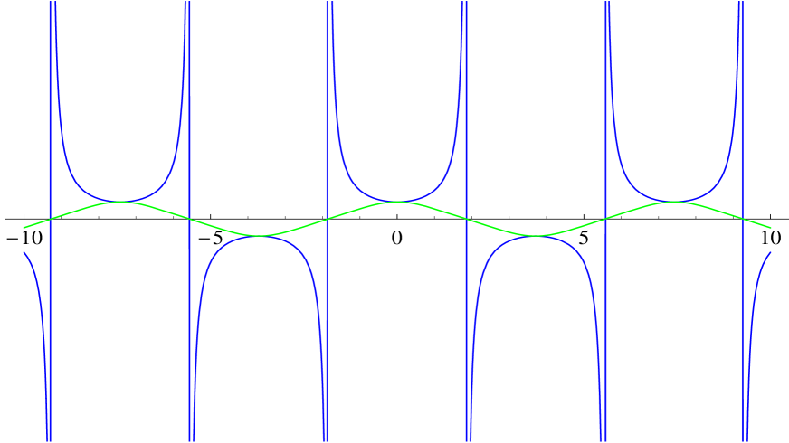
Figure 1: Analytic plot of the Jacobi elliptic function solution for the static fuzzy-$S^{2}$ funnel array and the collapsing 2-sphere for $r_{0}=1$.

2.3 An $r\rightarrow 1/r$ duality between the Euclidean and Lorentzian DBI equations

Defining $s={dr\over dt}$ the equation (2.23) can be written as

$$s^{2}={r_{0}^{4}-r^{4}\over 1+r_{0}^{4}}$$ (2.36)

Viewing $s$ and $r$ as two complex variables constrained by one equation, this defines a genus one Riemann surface. The quantity ${dr\over s}$ which gives the infinitesimal time elapsed is an interesting geometrical quantity related to the Riemann surface, i.e. the holomorphic differential.

The curve (2.36) has a number of automorphisms of interest. One checks that $R={r_{0}^{2}\over r}$, $\tilde{s}={isr_{0}^{2}\over r^{2}}$ leaves the equation of the curve invariant. This automorphism of the curve leads directly to the complex multiplication identity (2.31) which relates the spatial and time-dependent solutions. Another, not unrelated, automorphism acts as $R\rightarrow{1\over r}$, $R_{0}\rightarrow{1\over r_{0}}$, $\tilde{s}={is\over r^{2}}$. The relation between $\tilde{s}$ and $s$ is equivalent to a Wick rotation of the time variable. The transformation $r\rightarrow{1\over r}$ can also be taken to act on the second order equation since it does not involve $r_{0}$ (which does not appear in the second order equation). The spatial BPS solution to the second order equation can be acted upon by this transformation. The outcome is a time-dependent solution describing a brane collapsing at the speed of light $r=\pm(t-t_{\infty})$. This solution can be derived as a $r_{0}\rightarrow\infty$ limit of the general time-dependent elliptic solution, in much the same way as the BPS solution was derived as an $r_{0}\rightarrow 0$ limit of the spatial elliptic solutions.

The action of the $r\rightarrow{1\over r}$ transformation on the second order equations can be seen explicitly. In the case of pure time dependence, the equation of motion in dimensionless variables is

$$\ddot{r}=-2r^{3}\left({1-\dot{r}^{2}\over{1+r^{4}}}\right)\;,$$ (2.37)

while in the case of pure spatial dependence

$${r^{\prime\prime}}=2r^{3}\left({1+{r^{\prime}}^{2}\over 1+r^{4}}\right)\;.$$ (2.38)

A substitution $r=1/R$ can be used to transform (2.37) using

$$\displaystyle\dot{r} = -{1\over R^{2}}\dot{R}$$

$$\ddot{r} = -{1\over R^{2}}\ddot{R}+{2\over R^{3}}{\dot{R}}^{2}\;,$$

to get

$$-{\ddot{R}\over R^{2}}+{2\over R^{3}}(\dot{R})^{2}=-{2\over R^{3}}{1-{{\dot{R}}^{2}\over R^{4}}\over{1+1/R^{4}}}\;,$$ (2.39)

which can be simplified to

$$\ddot{R}=2R^{3}\left({1+\dot{R}^{2}\over 1+R^{4}}\right)\;.$$ (2.40)

So the effect of transforming $r\rightarrow{1\over r}$ and renaming $t\rightarrow\sigma$ is the same as the substitution $t\rightarrow i\sigma$. This explains the relation between (2.25) and (2.32) which was previously obtained using the complex multiplication property (2.31) of Jacobi-$Cn$ functions.

3 Space and Time dependent fuzzy $S^{4}$

3.1 Equivalence of the action for the $D1\perp D5$ intersection

We will extend the consideration of space and time dependent solutions to DBI for the case of the $D1\perp D5$ intersection, which involves a fuzzy $S^{4}$, generalising the purely spatial discussion of [2]. The equations are also relevant to the time-dependence of fuzzy spherical $D0$-$D4$ systems which have been studied in the Yang-Mills limit in [13]. On the $D1$ side, we will have five transverse scalar fields, satisfying the ansatz

$$\Phi^{i}(\sigma,\tau)=\pm\hat{R}(\sigma,\tau)G^{i},\qquad i=1,\ldots 5\;,$$ (3.1)

where the $G^{i}$’s are given by the action of $SO(5)$ gamma matrices on the totally symmetric $n$-fold tensor product of the basic spinor, the dimension of which is related to $n$ by

$$N=\frac{(n+1)(n+2)(n+3)}{6}\;.$$ (3.2)

The radial profile and the fuzzy-$S^{4}$ physical radius are again related by

$$R_{ph}(\sigma,\tau)=\sqrt{c}\lambda\hat{R}(\sigma,\tau)\;,$$ (3.3)

where $c$ is the ‘Casimir’ $G^{i}G^{i}=c\mathbf{1}_{N}=n(n+4)\mathbf{1}_{N\times N}$. By plugging the ansatz (3.1) into the action and by considering the large-$N$ behaviour of the configuration, one gets in dimensionless variables defined just as for the $S^{2}$ case in (2.10),

$$S_{1}=-N\;T_{1}\int d^{2}\sigma\sqrt{1+r^{\prime 2}-\dot{r}^{2}}\left(1+r^{4}\right)\;.$$ (3.4)

As in the $D1\perp D3$ case, we can write the equations of motion for this configuration in a Lorentz-invariant way. The result is the same as before with the exception of the pre-factor on the right-hand-side

$$\partial_{\mu}\partial^{\mu}r+(\partial_{\mu}\partial^{\mu}r)\;(\partial_{\nu}r)\;(\partial^{\nu}r)-(\partial_{\mu}\partial^{\nu}r)\;(\partial_{\nu}r)\;(\partial^{\mu}r)=4\;r^{3}\left(\frac{1+(\partial_{\mu}r)\;(\partial^{\mu}r)}{1+r^{4}}\right)\;,$$ (3.5)

where again $\mu$ and $\nu$ can take the values $\sigma,\tau$.

Let us now look at the $D5$ side: The world-volume action for $n$ $D5$-branes, with one transverse scalar excited, is as usual

$$S_{5}=-T_{5}\int d^{6}\sigma Str\sqrt{-det(G_{ab}+\lambda^{2}\partial_{a}\Phi\partial_{b}\Phi+\lambda F_{ab}})\;.$$ (3.6)

Introducing spherical co-ordinates with radius $R_{D5}$ and angles $\alpha^{i}$ ($i=1,\ldots,4$), we will have $ds^{2}=-dt^{2}+dR_{D5}^{2}+R_{D5}^{2}g_{ij}d\alpha^{i}d\alpha^{j}$, where $g_{ij}$ is the metric of a unit four-sphere, the volume of which is given by $\int d^{4}\alpha\sqrt{g}=8\pi^{2}/3$. We take the construction of [2] with homogeneous instantons and, keeping the same gauge field, we generalise $\Phi(R_{D5})$ to $\Phi(R_{D5},t)$. We will not review this here but just state that by using the above, we can reduce the previous expression to

$$S_{5}=-T_{5}\int d^{6}\sigma\sqrt{g}\sqrt{1+\lambda^{2}\Phi^{\prime 2}-\lambda^{2}\dot{\Phi}^{2}}\left(nR_{D5}^{4}+\frac{3}{2}N\lambda^{2}\right)\;,$$ (3.7)

Then by implementing once again the relations (2.18) we recover

$$S_{5}=-T_{5}\int d^{4}\alpha\wedge dt\wedge dR_{ph}\;\sqrt{g}\sqrt{1+\frac{1}{R_{ph}^{\prime 2}}-\frac{\dot{R}_{ph}^{2}}{R_{ph}^{\prime 2}}}\left(nR_{ph}^{4}+\frac{3}{2}N\lambda^{2}\right)\;.$$ (3.8)

This can be easily manipulated to yield the following result

$$S_{5}=-T_{1}N\int d\tau\wedge d\sigma\sqrt{1+R_{ph}^{\prime 2}-\dot{R}_{ph}^{2}}\left(1+\frac{2n}{3N\lambda^{2}}R_{ph}^{4}\right)\;.$$ (3.9)

Using $\frac{2n}{3N}\sim\frac{4}{c}$, which holds for large-$N$ and by once again employing dimensionless variables, this becomes

$$S_{5}=-T_{1}N\int d\tau\wedge d\sigma\sqrt{1+r^{\prime 2}-\dot{r}^{2}}\left(1+r^{4}\right)\;,$$ (3.10)

which agrees with (3.4) and can be further simplified to the re-scaled action

$$\tilde{S}_{5}=-\int d^{2}\sigma\sqrt{1+r^{\prime 2}-\dot{r}^{2}}(1+r^{4})\;.$$ (3.11)

Thus, every space-time dependent solution described by the DBI equations of motion from the D1 worldvolume will have an equivalent description on the D5 worldvolume.

3.2 Solutions for the space-dependent fuzzy spheres: Funnels

Assuming $\dot{r}=0$, the action (3.11) becomes

$$\tilde{S}_{5}=-\int d^{2}\sigma\sqrt{1+{r^{\prime}}^{2}}~{}~{}(1+r^{4})\;.$$ (3.12)

There exists a conserved pressure $T^{\sigma\sigma}=P$ given by

$$P={1+r^{4}\over\sqrt{1+{r^{\prime}}^{2}}}\;,$$ (3.13)

which can be solved to give ${r^{\prime}}$

$$\displaystyle\left({dr\over d\sigma}\right)^{2} = {{1\over P^{2}}-1}+{(1+r^{4})^{2}\over P^{2}}$$

$$= {(2r^{4}+r^{8})-(2r_{0}^{4}+r_{0}^{8})\over(1+r_{0}^{4})^{2}}\;.$$

Defining ${dr\over d\sigma}=s$ this can be expressed as

$$s^{2}={(r^{4}-r_{0}^{4})(r^{4}-r_{1}^{4})\over(1+r_{0}^{4})^{2}}$$ (3.14)

The roots in the equation above correspond to $(1+r^{4})=(1+r_{0}^{4})$ and $(1+r^{4})=-(1+r_{0}^{4})$. The second possibility gives $r_{1}^{4}=-2-r_{0}^{4}$. By differentiating the pressure, a second order differential equation can be derived

$$\displaystyle{d^{2}r\over d\sigma^{2}} = {4r^{3}(1+{r^{\prime}}^{2})\over(1+r^{4})}$$ (3.15)

$$= {4r^{3}(1+r^{4})\over P^{2}}\;.$$

An integral formula can be written for the distance along the $D1$-brane using (3.2)

$$\int_{0}^{\sigma}d\sigma=\int_{r_{0}}^{r}dr{(1+r_{0}^{4})\over\sqrt{(2r^{4}+r^{8})-(2r_{0}^{4}+r_{0}^{8})}}\;,$$ (3.16)

where we have taken the zero of $\sigma$ to be at the place $r=r_{0}$ where ${r^{\prime}}=0$. We deduce from the integral that there is a finite value of $\sigma$, denoted as $\Sigma$, where $r$ has increased to infinity. This is similar to part of the spatial solution of the $D1$-$D3$ system described by the $Cn$ function (see Figure 1). We can show that the full periodic structure analogous to that of the spatial $D1$-$D3$ system follows in the $D1$-$D5$ system, by using symmetries of the equations and the requirement that the derivative ${dr\over d\sigma}$ is continuous. Note that (3.2) is symmetric under the operations

$$I_{\sigma}:r(\sigma)\rightarrow r(-\sigma)$$

$$I_{r}:r(\sigma)\rightarrow-r(\sigma)$$

$$T_{\Sigma}:r(\sigma)\rightarrow r(\sigma-\Sigma)\>.$$ (3.17)

The branch with $r$ increasing from $r_{0}$ to $\infty$, as $\sigma$ changes from $0$ to $\Sigma$, can be acted on by $T_{2\Sigma}I_{\sigma}I_{r}$ to yield a branch where $r$ increases from $-\infty$ to $-r_{0}$ over $\Sigma\leq\sigma\leq 2\Sigma$. Acting with $T_{2\Sigma}I_{r}$ gives a branch where $r$ decreases from $-r_{0}$ to $-\infty$ over $2\Sigma\leq\sigma\leq 3\Sigma$. Finally a transformation of the original branch by $T_{4\Sigma}I_{\sigma}$ gives $r$ decreasing from $\infty$ to $r_{0}$ over $3\Sigma\leq\sigma\leq 4\Sigma$. These four branches patch together without discontinuity in $r$ or ${dr\over d\sigma}$ and can further be translated by integer multiples of $4\Sigma$, to give a picture qualitatively similar to the $D1$-$D3$ case, but now describing $D1$ funnels between alternating $D5$ and anti-$D5$. The profile has the properties

$$\displaystyle r(\sigma+2\Sigma) = -r(\sigma)$$

$$r(\sigma+4m\Sigma) = r(\sigma)$$

$${1\over{r(~{}(2m+1)\Sigma~{})}} = 0\;,$$ (3.18)

where $m$ is an arbitrary integer. This picture, including the poles and periodicity, will be recovered with an improved quantitative description of $r$ as a function of complex arguments in section 4 (see Figure 2).

3.3 Solutions for the time-dependent fuzzy spheres: Collapsing spheres

In the time-dependent case, there is a conserved energy

$$E={(1+r^{4})\over\sqrt{(1-\dot{r}^{2})}}\;.$$ (3.19)

implying

$$(1+r_{0}^{4})^{2}={(1+r^{4})^{2}\over(1-\dot{r}^{2})}\;.$$ (3.20)

This can be solved for the velocity

$$\displaystyle\left({dr\over dt}\right)^{2} = {1-{1\over E^{2}}}-{1\over E^{2}}(2r^{4}+r^{8})$$

$$= {(2r_{0}^{4}+r_{0}^{8})-(2r^{4}+r^{8})\over(1+r_{0}^{4})^{2}}\;.$$

Writing $s={dr\over dt}$

$$\displaystyle s^{2} = {(1+r_{0}^{4})^{2}-(1+r^{4})^{2}\over(1+r_{0}^{4})^{2}}$$ (3.21)

$$= {-(r^{4}-r_{0}^{4})(r^{4}-r_{1}^{4})\over(1+r_{0}^{4})^{2}}\;.$$ (3.22)

A trivial redefinition $s\rightarrow is$ relates the equation (3.22) to (3.14). The time evolved can be written in terms of the radial distance

$$\int_{0}^{t}dt=\int_{r_{0}}^{r}dr{(1+r_{0}^{4})\over\sqrt{(2r_{0}^{4}+r_{0}^{8})-(2r^{4}+r^{8})}}\;.$$ (3.23)

Differentiating (3.3) gives a second order equation

$$\displaystyle\ddot{r} = {-4r^{3}(1+r^{4})\over E^{2}}$$ (3.24)

$$= {-4r^{3}(1+r^{4})\over(1+r_{0}^{4})^{2}}\;.$$

We can see from (3.23) that the time taken to start from $r=r_{0}$ and reach $r=0$ is finite. We will call this finite time interval the time of collapse $T$. As in the spatial problem there are symmetries of the equation

$$I_{t}:r(t)\rightarrow r(-t)$$

$$I_{r}:r(t)\rightarrow-r(t)$$

$$T_{T}:r(t)\rightarrow r(t-T)\;.$$ (3.25)

Following the same steps as in the spatial case, we can act successively with $I_{2\Sigma}I_{t}I_{r}$ , $I_{2\Sigma}I_{r}$, $I_{3\Sigma}I_{t}$ and then with integer multiples of $4T$ to produce a periodic solution defined for positive and negative time. As discussed before and in analogy to the $D1$-$D3$ scenario, this can be interpreted in terms of collapsing-expanding $D4$-branes. The radius as a function of $t$ has the properties

$$\displaystyle r(t+4mT) = r(t)$$

$$r(T)=r(~{}(2m+1)T~{}) = 0$$

$$r(t+2mT) = -r(t)\;,$$ (3.26)

where $m$ is an arbitrary integer. We will see in the following that it will be useful to define a complex variable $u_{1}$ whose real part is related to $\sigma$ and whose imaginary part is related to $t$ as $u_{1}=\sigma-it$. Unlike the case of the fuzzy two-sphere, we are not dealing simply with a variable $u$ living on a torus. Rather it will become necessary to introduce a second complex variable $u_{2}$ such that the pair $(u_{1},u_{2})$ lives on the Jacobian of a genus two-curve. It will also be natural to impose a constraint which amounts to looking at sub-varieties of the Jacobian. At the end of this it will, nevertheless, be possible to recover the sequence of zeroes and poles in (3.3) and (3.2).

3.4 Geometry and Automorphisms of Hyper-elliptic curve for the fuzzy $S^{4}$

The equation (3.22) defines a Riemann surface of genus $3$. The integrals of interest (3.16) and (3.23), are integrals of a holomorphic differential along certain cycles of the Riemann surface. It is useful to recall the Riemann-Hurwitz formula

$$(2g-2)=n(2G-2)+B\;,$$ (3.27)

which gives the genus $g$ of the covering surface in terms of the genus $G$ of the target and the number of branch points $B$. Since the RHS of (3.22) is a polynomial of degree $8$ there are $8$ points where $s=0$, i.e. $8$ branch points. Here $G=0$ since the $r$ co-ordinate can be viewed as living on the sphere, $n=2$ and $B=8$. So the integrals are defined on a genus $g=3$ curve, which we will call $\Sigma_{3}$.

After dividing out by $r_{0}^{8}$ on both sides of (3.22) and rescaling $s={r_{0}^{4}{\tilde{s}}\over 1+r_{0}^{4}}$, $r^{4}=r_{0}^{4}{\tilde{r}}^{4}$, $r_{1}^{4}=r_{0}^{4}{\tilde{r}}_{1}^{4}$ we have

$$\tilde{s}^{2}=({\tilde{r}}^{4}-1)({\tilde{r}}^{4}-{\tilde{r}_{1}}^{4})\;.$$ (3.28)

There are three independent holomorphic differentials on this curve $\omega_{1}={d{\tilde{r}}\over{\tilde{s}}},\omega_{2}={{\tilde{r}}d{\tilde{r}}\over{\tilde{s}}},\omega_{3}={{\tilde{r}}^{2}d{\tilde{r}}\over{\tilde{s}}}$ (see for example [14, 15]). The infinitesimal time elapsed is $dt={dr\over s}={(1+r_{0}^{4})\over r_{0}^{3}}{d\tilde{r}\over\tilde{s}}$. It will be important in calculating the integrals (3.23)(3.16), to understand the automorphisms of the Riemann surface $\Sigma_{3}$. In the limit of large $r_{0}$, ${{\tilde{r}}_{1}}^{4}$ approaches $-1$ and there is an automorphism

$${\tilde{r}}\rightarrow{1\over{\tilde{r}}}$$

$${\tilde{s}}\rightarrow{i{\tilde{s}}\over{\tilde{r}}^{4}}\;,$$

which leaves the equation of the curve unchanged. It transforms the holomorphic differentials as follows

$$\omega_{1} \rightarrow i\omega_{3}$$

$$\omega_{2} \rightarrow i\omega_{2}$$

$$\omega_{3} \rightarrow i\omega_{1}\;.$$

For any finite $r_{0}$ there is a $Z_{2}$ automorphism, ${{\tilde{r}}}\rightarrow-{{\tilde{r}}}$. Quotienting by this can be achieved by changing variables ${{\tilde{r}}}^{2}=x$. The first and third holomorphic differentials $\omega_{1}$ and $\omega_{3}$ transform as follows

$${d{{\tilde{r}}}\over\sqrt{({\tilde{r}}^{4}-1)({\tilde{r}}^{4}-{\tilde{r}_{1}}^{4})}}={dx\over\sqrt{4x(x^{2}-1)(x^{2}-{\tilde{r}_{1}}^{4})}}$$

$${{\tilde{r}}^{2}d{{\tilde{r}}}\over\sqrt{({\tilde{r}}^{4}-1)({\tilde{r}}^{4}-{\tilde{r}_{1}}^{4})}}={xdx\over\sqrt{4x(x^{2}-1)(x^{2}-{\tilde{r}_{1}}^{4})}}\;.$$ (3.29)

We can view this in terms of a map from a genus three curve $({\tilde{r}},{\tilde{s}})$ to a genus two curve $(x,y)$

$$\displaystyle x = {\tilde{r}}^{2}$$

$$y = 2{\tilde{r}}{\tilde{s}}\;,$$ (3.30)

which implies

$$y^{2}=4{\tilde{r}}^{2}({\tilde{r}}^{4}-1)({\tilde{r}}^{4}-{{\tilde{r}_{1}}}^{4})=4x(x^{2}-1)(x^{2}-{{\tilde{r}_{1}}}^{4})\;.$$ (3.31)

This genus $2$ curve $(x,y)$ will be called $\Sigma_{2}$. The holomorphic differentials are related by ${d{\tilde{r}}\over{\tilde{s}}}={dx\over y}$ and ${{\tilde{r}}^{2}d{\tilde{r}}\over{\tilde{s}}}={xdx\over y}$. The map (3.30) has branching number $B=0$, in agreement with (3.27). Even though ${\partial x\over\partial{\tilde{r}}}=0$ at ${\tilde{r}}=0$, this is not a branch point, since $x$ is not a good local co-ordinate for the curve $(x,y)$ at $x=0$. Rather, a good local co-ordinate is $y$ which is linearly related to ${\tilde{r}}$ and this means that there is no branch point.

The second holomorphic differential transforms as

$${{\tilde{r}}d{\tilde{r}}\over\sqrt{({\tilde{r}}^{4}-1)({\tilde{r}}^{4}-r_{1}^{4})}}={dx\over 2\sqrt{(x^{2}-1)(x^{2}-{\tilde{r}_{1}}^{4})}}\;.$$ (3.32)

This can be viewed in terms of a map

$$\displaystyle\tilde{x} = {\tilde{r}}^{2}$$

$$\tilde{y} = {\tilde{s}}$$ (3.33)

to a target torus $(\tilde{x},\tilde{y})$, obeying

$${\tilde{y}}^{2}=({\tilde{x}}^{2}-1)({\tilde{x}}^{2}-{\tilde{r}_{1}}^{4})\;.$$ (3.34)

This map has $B=4$, again in agreement with (3.27). There are two branch points at $({\tilde{r}},{\tilde{s}})=(0,\pm{{\tilde{r}_{1}}}^{2})$ corresponding to $(\tilde{x},\tilde{y})=(0,\pm{{\tilde{r}_{1}}}^{2})$. Similarly we have two branch points at ${\tilde{r}}=\infty$. The region near ${\tilde{r}}=\infty$ is best studied by defining variables $\hat{r}={{\tilde{r}}}^{-1}$ and $\hat{s}={{\tilde{s}}{{\tilde{r}}}^{-4}}$ which re-express (3.28) as $\hat{s}^{2}=(1-\hat{r}^{4})(1-\hat{r}^{4}{{\tilde{r}_{1}}}^{4})$. Similarly we define $\hat{x}={\tilde{x}}^{-1},\hat{y}=\tilde{y}{\tilde{x}}^{-2}$ which re-expresses (3.34) as $\hat{y}^{2}=(1-\hat{x}^{2})(1-\hat{x}^{2}{\tilde{r}_{1}}^{4})$. Two branch points corresponding to ${\tilde{r}}=\infty$ are at $(\hat{x},\hat{y})=(0,\pm 1)$.

The genus two curve $\Sigma_{2}$ itself can be related to genus one curves. We first rewrite the $(x,y)$ equation (3.31) as

$$\displaystyle y^{2}=4x(x-1)(x+1)(x-iR_{1}^{2})(x+iR_{1}^{2})\;,$$ (3.35)

with $R_{1}^{2}=-i{\tilde{r}}_{1}^{2}$ and real. This is of the special form [16, 17]

$$y^{2}=x(x-1)(x-\alpha)(x-\beta)(x-\alpha\beta)\;,$$ (3.36)

with $\alpha=-1$ and $\beta=iR_{1}^{2}$. Such curves have an automorphism $T_{1}$

$$T_{1}(x)\equiv X={\alpha\beta\over x}={-iR_{1}^{2}\over x}$$

$$T_{1}(y)\equiv Y={(\alpha\beta)^{3\over 2}y\over x^{3}}={e^{i\pi\over 4}R_{1}^{3}y\over x^{3}}\;,$$ (3.37)

which transforms the holomorphic differentials

$$\displaystyle T_{1}\left({dx\over y}\right) ={iXdX\over Y\sqrt{\beta}}$$

$$T_{1}\left({xdx\over y}\right) ={-i\sqrt{\beta}dX\over Y}\;.$$ (3.38)

The genus two curve (3.35) can be put in the form (3.36) in yet another way, by choosing $\alpha=-1$, $\beta=-iR_{1}^{2}$. This gives another automorphism $T_{2}$ which acts as

$$\displaystyle T_{2}(x)={iR_{1}^{2}\over x}$$

$$T_{2}(y)={e^{3i\pi\over 4}yR_{1}^{3}\over x^{3}}\;.$$ (3.39)

With either choice of $(\alpha,\beta)$ one is led to look for variables which are invariant under the automorphism and as a result one describes the genus $2$ curve as a covering of two genus one curves $(\xi_{\pm},\eta_{\pm})$ [16, 17]

$$\eta_{\pm}^{2}=\xi_{\pm}(1-\xi_{\pm})(1-k_{\pm}^{2}\xi_{\pm})\quad\textrm{with}\quad k_{\pm}^{2}=-\frac{(\sqrt{\alpha}\mp\sqrt{\beta})^{2}}{(1-\alpha)(1-\beta)}\;.$$ (3.40)

The maps are given by

$$\displaystyle\xi_{\pm} = \frac{(1-\alpha)(1-\beta)x}{(x-\alpha)(x-\beta)}$$

$$\eta_{\pm} = -\sqrt{(1-\alpha)(1-\beta)}{x\mp\sqrt{\alpha\beta}\over(x-\alpha)^{2}(x-\beta)^{2}}y\;.$$ (3.41)

This gives an isomorphism of the Jacobian of the genus 2 curve in terms of a product of the Jacobians of the genus $1$ curves $\Sigma_{\pm}$. For the case $\alpha=-1$ we have $K(k_{+})=K^{\prime}(k_{-})$. Since the complex structure is $\tau=i{K^{\prime}(k)\over K(k)}$, this means that the complex structures of $\Sigma_{+}$ and $\Sigma_{-}$ are related by the $SL(2,\mathbb{Z})$ transformation $\tau\rightarrow-{1\over\tau}$. Hence $\Sigma_{\pm}$ have isomorphic complex structures.

As an aside we describe the full group of automorphisms of $\Sigma_{2}$. It includes $\sigma$, the hyperelliptic involution, $\sigma(x)=x,\sigma(y)=-y$ ; $T_{3}$, which acts as $T_{3}(x)=-x,T_{3}(y)=-iy$, and $T_{4}$, which acts as $T_{4}(x)=-x,T_{4}(y)=iy$. Relations in this group of automorphisms are

$$\displaystyle T_{1}T_{2} = T_{3}$$

$$T_{2}T_{1} = T_{4}$$

$$T_{3}T_{4}=T_{4}T_{3} = 1$$

$$T_{3}^{2} = \sigma$$

$$T_{3}\sigma = T_{4}\;.$$ (3.42)

In the limit $r_{0}\rightarrow\infty$, $R_{1}=1$ and the equation for the curve simplifies

$$y^{2}=x(x^{4}-1)\;.$$ (3.43)

As a result, the automorphism group is larger than at finite $r_{0}$. The automorphism group is generated by $U_{1}$ and $U_{2}$ which act as follows

$$\displaystyle U_{1}(x) = {1\over x}$$

$$U_{1}(y) = {e^{i\pi\over 2}y\over x^{3}}$$

$$U_{2}(x) = e^{i\pi\over 2}x$$

$$U_{2}(y) = e^{i\pi\over 4}y\;.$$ (3.44)

If we write $U_{1}(x)=X,U_{1}(y)=Y$, we have the following action on the holomorphic differentials

$$\displaystyle{dx\over y} = -i{XdX\over y}$$

$${xdx\over y} = -i{dX\over Y}\;.$$ (3.45)

The action of $U_{2}$ on the holomorphic differentials is just

$$\displaystyle{dx\over y} \rightarrow{e^{-i\pi\over 4}dx\over y}$$

$${xdx\over y} \rightarrow{e^{-3i\pi\over 4}xdx\over y}\;.$$ (3.46)

The automorphism group includes, as usual, the hyperelliptic involution acting as $\sigma(x)=x,\sigma(y)=-y$. There is also an element $U_{3}$ acting as $U_{3}(x)=-x,U_{3}(y)=iy$. There are relations $U_{1}^{2}=\sigma,U_{2}^{2}=U_{3}$. In the large $r_{0}$ limit, $R_{1}\rightarrow 1$, the formulae for $T_{1},T_{2}$ from (3.37),(3.39) simplify and they can be written in terms of $U_{1},U_{2}$. Indeed we find that

$$\displaystyle T_{1} = \sigma U_{2}U_{1}$$

$$T_{2} = \sigma U_{2}^{-1}U_{1}\;.$$

3.5 Evaluation of integrals

The time integral (3.23) can be done in terms of Appell functions. The indefinite integral is

$${(1+r_{0}^{4})r\over\sqrt{(2r_{0}^{4}+r_{0}^{8})}}F_{1}\left({1\over 4};{1\over 2},{1\over 2};{5\over 4};{r^{4}\over r_{0}^{4}},-{r^{4}\over{2+r_{0}^{4}}}\right)\;.$$ (3.47)

A quick way to get this is by using the Integrator [18] but we outline a derivation. Expanding the integrand of (3.23)

$$\int dr(r_{0}^{4}-r^{4})^{-{1\over 2}}(r_{0}^{4}+2+r^{4})^{-{1\over 2}}$$

$$=r_{0}^{-2}(2+r_{0}^{4})^{-\frac{1}{2}}\int dr\sum_{k,l=0}^{\infty}{\Gamma({1\over 2})\over\Gamma({1\over 2}-k)\Gamma(k+1)}{\Gamma({1\over 2})\over\Gamma({1\over 2}-l)\Gamma(l+1)}(-1)^{k}\left({r\over r_{0}}\right)^{4k}\left({r^{4}\over 2+r_{0}^{4}}\right)^{l}$$

$$=r_{0}^{-2}(2+r_{0}^{4})^{-{1\over 2}}\;r\sum_{k,l=0}^{\infty}{1\over k!l!}{\Gamma({1\over 2})\over\Gamma({1\over 2}-k)}{\Gamma({1\over 2})\over\Gamma({1\over 2}-l)}{1\over 4k+4l+1}(-1)^{k}\left({r\over r_{0}}\right)^{4k}\left({r^{4}\over 2+r_{0}^{4}}\right)^{l}\;.$$

Now use the following facts about $\Gamma$ functions

$${\Gamma({1\over 2})\over\Gamma({1\over 2}-k)}=(-1)^{k}{\Gamma({1\over 2}+k)\over\Gamma({1\over 2})}$$

$${\Gamma({1\over 2})\over\Gamma({1\over 2}-l)}=(-1)^{l}{\Gamma({1\over 2}+l)\over\Gamma({1\over 2})}$$

$${1\over 4(k+l+{1\over 4})}={\Gamma({5\over 4})\over\Gamma({1\over 4})}{\Gamma({1\over 4}+k+l)\over\Gamma({5\over 4}+k+l)}\;,$$

to recognise the series expansion of the Appell function [19]

$$F_{1}(a;b_{1},b_{2};c;z_{1},z_{2})=\sum_{k=0}^{\infty}\sum_{l=0}^{\infty}{(a)_{k+l}(b_{1})_{k}(b_{2})_{l}z_{1}^{k}z_{2}^{l}\over(c)_{k+l}k!l!}\;,$$ (3.48)

with arguments as given in (3.47) and where we have also made use of the Pochhammer symbols $(a)_{n}=\frac{\Gamma(a+n)}{\Gamma(a)}$.

Using (3.47), the time taken to collapse from the initial radius $r_{0}$ to a smaller radius $r$ is

$$t={(1+r_{0}^{4})r_{0}\over\sqrt{(2r_{0}^{4}+r_{0}^{8})}}F_{1}\left({1\over 4};{1\over 2},{1\over 2};{5\over 4};1,-{r_{0}^{4}\over{2+r_{0}^{4}}}\right)-{(1+r_{0}^{4})r\over\sqrt{(2r_{0}^{4}+r_{0}^{8})}}F_{1}\left({1\over 4};{1\over 2},{1\over 2};{5\over 4};{r^{4}\over r_{0}^{4}},-{r^{4}\over{2+r_{0}^{4}}}\right)\;.$$ (3.49)

For the special values $r=r_{0}$, $z_{1}=1$, $F_{1}$ of (3.47) simplifies to

$${(1+r_{0}^{4})\over r_{0}\sqrt{(2+r_{0}^{4})}}~{}~{}{}_{2}F_{1}\left({1\over 4},{1\over 2};{5\over 4};1\right)~{}~{}{}_{2}F_{1}\left({1\over 4},{1\over 2};{3\over 4};-{r_{0}^{4}\over 2+r_{0}^{4}}\right)\;.$$ (3.50)

For $r=0$, $F_{1}=1$ and the indefinite integral (3.47) evaluates to zero. Hence the time of collapse is given by (3.50) which can be simplified to

$$T={(1+r_{0}^{4})\over r_{0}\sqrt{(2+r_{0}^{4})}}{\Gamma({5\over 4})\Gamma({1\over 2})\over{\Gamma({3\over 4})}}{}_{2}F_{1}\left({1\over 4},{1\over 2};{3\over 4};{-r_{0}^{4}\over 2+r_{0}^{4}}\right)\;.$$ (3.51)

For large $r_{0}$ the last argument of the hypergeometric function simplifies to $-1$ and we get

$$T=r_{0}{\Gamma({5\over 4})\Gamma({1\over 2})\over\Gamma({3\over 4})}{2^{-1/4}\Gamma({3\over 4})\over{\Gamma({5\over 8})\Gamma({5\over 8})}}=r_{0}\sqrt{\pi}{\Gamma({9\over 8})\over\Gamma({5\over 8})}\sim 1.1636...~{}~{}r_{0}\;.$$ (3.52)

It is also of interest to compute the interval in $\sigma$ along the D-string from the minimum size of the funnel cross-section to the place where the funnel blows up. The indefinite integral (3.16) gives by direct evaluation, just as above

$$\frac{i\;(1+r_{0}^{4})}{r_{0}^{2}}\frac{r}{\sqrt{2+r_{0}^{4}}}F_{1}\left(\frac{1}{4},\frac{1}{2},\frac{1}{2},\frac{5}{4};\frac{r^{4}}{r_{0}^{4}},-\frac{r^{4}}{2+r_{0}^{4}}\right)\;.$$ (3.53)

The distance to blow-up is given by the difference of the last expression evaluated at infinity and at $r_{0}$. We do not have an exact formula for the large $r$ asymptotics of the Appell function at finite $r_{0}$. We will thus be forced to take the large $r_{0}$ limit immediately. This will reduce (3.53) to

$$i\;r_{0}\;r\;{}_{2}F_{1}\left(\frac{1}{8},\frac{1}{2},\frac{9}{8};\frac{r^{8}}{r_{0}^{8}}\right)$$ (3.54)

and the distance to blow-up will be

$$\frac{i\;r_{0}\;\Gamma(\frac{3}{8})\Gamma(\frac{9}{8})}{\sqrt{\pi}(-1)^{1/8}}-\frac{i\;r_{0}\;\sqrt{\pi}\Gamma(\frac{9}{8})}{\Gamma(\frac{5}{8})}\;.$$ (3.55)

The final result is

$$\Sigma=r_{0}(\sqrt{2}-1)\sqrt{\pi}\frac{\Gamma(\frac{9}{8})}{\Gamma(\frac{5}{8})}\sim 0.4819..r_{0}\;.$$ (3.56)

Hence the full period $4\Sigma$ is $1.9276..r_{0}$. The time of collapse is $1.1636...r_{0}$. The space and time periods are no longer the same as was the case for fuzzy $S^{2}$, since there is a relative factor of $(\sqrt{2}-1)$.

4 Reduction of the $g=3$ curve and inversion of the hyper-elliptic integral for the fuzzy-$S^{4}$

Whereas we have formulae for the time elapsed $t$ in terms of $r$ (3.49) or the D1-co-ordinate $\sigma$ as a function of $r$ by using (3.53), it is desirable to have the inverse formulae expressing $r$ as a function of $\sigma$ and $t$. It will turn out that, as in the case of the fuzzy $S^{2}$, it will be useful to define a complex variable $u_{1}=\sigma-it$. Whereas the $u$ variable in the case of fuzzy $S^{2}$ lives on a genus one curve, here the story will involve higher genus curves and will require the introduction of a second complex variable $u_{2}$.

Let us revisit the $\sigma$-integral in the case of the fuzzy-$S^{4}$. The integral we want to perform is

$$\sigma=\int_{r_{0}}^{r}\frac{(1+r_{0}^{4})dr}{\sqrt{(r^{4}-r_{0}^{4})(r^{4}-r_{1}^{4})}}$$

with $r_{1}^{4}=-(2+r_{0}^{4})$. If we make the re-scaling $\tilde{r}=\frac{r}{r_{0}}$ and $\tilde{r}_{1}=-\frac{2+r_{0}^{4}}{r_{0}^{4}}$ we get

$$\frac{\sigma r_{0}^{3}}{(1+r_{0}^{4})}=\int_{1}^{\tilde{r}}\frac{d\tilde{r}}{\sqrt{(\tilde{r}^{4}-1)(\tilde{r}^{4}-\tilde{r}_{1}^{4})}}\;.$$ (4.1)

The RHS is the integral over the holomorphic differential on $\Sigma_{3}$ of section $3.4$. Using the reduction to $\Sigma_{2}$ by making a change of variables $\tilde{r}^{2}=x$, we arrive at

$$\frac{2r_{0}^{3}\;\sigma}{(1+r_{0}^{4})}=\int_{1}^{x}\frac{dx}{\sqrt{x(x^{2}-1)(x^{2}-\tilde{r}_{1}^{4})}}\;.$$ (4.2)

Similar steps for the time-dependent fuzzy-sphere give

$$-i\frac{2r_{0}^{3}\;t}{(1+r_{0}^{4})}=\int_{1}^{x}\frac{dx}{\sqrt{x(x^{2}-1)(x^{2}-{\tilde{r}}_{1}^{4})}}\;.$$ (4.3)

At this point it is useful to introduce a complex variable $u_{1}=\sigma-it$. The inversion of the integrals (4.2), (4.3) is related to the Jacobi inversion problem

$$\displaystyle\int_{x_{0}}^{x_{1}}\frac{dx}{y}+\int_{x_{0}}^{x_{2}}\frac{dx}{y} = u_{1}$$

$$\int_{x_{0}}^{x_{1}}\frac{xdx}{y}+\int_{x_{0}}^{x_{2}}\frac{xdx}{y} = u_{2}\;,$$ (4.4)

where $x_{0}$ is any fixed point on the Riemann surface $\Sigma_{2}$. We will set $x_{0}=1$. By further fixing $x_{2}=1$ we recover the integral of interest in the first line

$$\displaystyle\int_{1}^{x_{1}}\frac{dx}{y} = u_{1}$$

$$\int_{1}^{x_{1}}\frac{xdx}{y} = u_{2}\;,$$ (4.5)

This is a constrained Jacobi inversion problem which is related to a sub-variety of the Jacobian of $\Sigma_{2}$, denoted as $J(\Sigma_{2})$. A naive attempt to consider the inversion of the first equation of (4) in isolation runs into difficulties with infinitesimal periods as explained on page 238 of [15].

By switching to the variables $\xi_{\pm},\eta_{\pm}$ defined in (3.41), the system (4) can be reduced to the sum of simple elliptic integrals

$$\displaystyle\int_{\xi_{0}}^{\xi_{1}}\frac{d\xi_{+}}{\eta_{+}}+\int_{\xi_{0}}^{\xi_{2}}\frac{d\xi_{+}}{\eta_{+}} = u_{+}$$

$$\int_{\xi_{0}}^{\xi_{1}}\frac{d\xi_{-}}{\eta_{-}}+\int_{\xi_{0}}^{\xi_{2}}\frac{d\xi_{-}}{\eta_{-}} = u_{-}\;,$$ (4.6)

where $\xi_{1}=\xi_{\pm}(x_{1})$ and $\xi_{2}=\xi_{\pm}(x_{2})$. We have used

$$\frac{d\xi_{\pm}}{\eta_{\pm}}=\sqrt{(1-\alpha)(1-\beta)}(x\pm\sqrt{\alpha\beta})\frac{dx}{y}\quad\textrm{and}\quad u_{\pm}=\sqrt{(1-\alpha)(1-\beta)}(u_{2}\pm\sqrt{\alpha\beta}\;u_{1})\;.$$ (4.7)

The first of the two integrals can be brought into the form

$$\int_{1}^{\sqrt{\xi_{1}}}\frac{2dz}{\sqrt{(1-z^{2})(1-k_{+}^{2}z^{2})}}+\int_{1}^{\sqrt{\xi_{2}}}\frac{2dz}{\sqrt{(1-z^{2})(1-k_{+}^{2}z^{2})}}=u_{+}\;,$$ (4.8)

by the substitution $\xi=z^{2}$ and then split to give

$$\displaystyle 2\int_{0}^{\sqrt{\xi_{1}}}\frac{dz}{\sqrt{(1-z^{2})(1-k_{+}^{2}z^{2})}} + 2\int_{0}^{\sqrt{\xi_{2}}}\frac{dz}{\sqrt{(1-z^{2})(1-k_{+}^{2}z^{2})}}$$ (4.9)

$$- 4\int_{0}^{1}\frac{dz}{\sqrt{(1-z^{2})(1-k_{+}^{2}z^{2})}}=u_{+}\;,$$

which are just

$$2Sn^{-1}(\sqrt{\xi_{1}},k_{+})+2Sn^{-1}(\sqrt{\xi_{2}},k_{+})-4K(k_{+})=u_{+}\;.$$ (4.10)

Then by using the addition formulae for $Sn^{-1}$ functions [22], we arrive at

$$Sn^{-1}\left(\frac{\sqrt{\xi_{1}}\sqrt{(1-\xi_{2})(1-k_{+}^{2}\xi_{2})}+\sqrt{\xi_{2}}\sqrt{(1-\xi_{1})(1-k_{+}^{2}\xi_{1})}}{1-k_{+}^{2}\xi_{1}\xi_{2}},k_{+}\right)=\frac{u_{+}}{2}+2K(k_{+})\;.$$ (4.11)

Thus by setting $x_{2}=1$ we get $\xi_{2}=1$ and

$$\frac{1-\xi_{1}}{1-k_{+}^{2}\xi_{1}}=Sn^{2}\left(\frac{u_{+}}{2}+2K(k_{+}),k_{+}\right)\;.$$ (4.12)

After using the fact that $Sn$ is anti-periodic in $2K(k)$ and implementing half-argument formulae, we end up with

$$\frac{1+Cn(u_{+},k_{+})}{1+Dn(u_{+},k_{+})}=\xi_{1}\;.$$ (4.13)

Starting from the second integral of (4) the same steps lead to

$$\frac{1+Cn(u_{-},k_{-})}{1+Dn(u_{-},k_{-})}=\xi_{1}\;.$$ (4.14)

These expressions hold the answer to the Jacobi inversion problem, although we still need to decouple $u_{1}$ and $u_{2}$ in the $u_{\pm}$’s.

4.1 Series expansion of $u_{2}$ as a function of $u_{1}$

The equations (4.13) and (4.14) imply that $u_{+}$ and $u_{-}$ are constrained by

$$\xi_{1}=\frac{1+Cn(u_{+},k_{+})}{1+Dn(u_{+},k_{+})}=\frac{1+Cn(u_{-},k_{-})}{1+Dn(u_{-},k_{-})}\;.$$ (4.15)

This can be used to solve for $u_{2}(u_{1})$ (or $u_{1}(u_{2})$). We do not have an explicit general solution to this transcendental constraint but we can solve it in a series around the initial radius $x=1$. This corresponds to small times, i.e. corresponds to doing perturbation theory for $u_{1}$ around zero and similarly for $u_{2}$, as can be seen from the integrals (4). We find

$$\displaystyle u_{2} = u_{1}+\frac{1}{6}(1+R_{1}^{4})u_{1}^{3}+\frac{1}{120}(1+R_{1}^{4})(7+3R_{1}^{4})u_{1}^{5}$$ (4.16)

$$+\frac{1}{2520}(1+R_{1}^{4})(65+66R_{1}^{4}+9R_{1}^{8})u_{1}^{7}+\mathcal{O}(u_{1}^{9})\;.$$

As a consistency check, we can invert the two integrals independently and see whether the expansion (4.16) agrees with the results.

In more detail we have

$$\int_{1}^{x_{1}}\frac{dx}{\sqrt{x(x^{2}-1)(x^{2}+R_{1}^{4})}}=u_{1}\;,$$

which can be expanded and inverted to give

$$\displaystyle x_{1} = \frac{1}{2}(1+R_{1}^{4})u_{1}^{2}+\frac{1}{24}(1+R_{1}^{4})(7+3R_{1}^{4})u_{1}^{4}+\frac{1}{360}(1+R_{1}^{4})(65+66R_{1}^{4}+9R_{1}^{8})u_{1}^{6}$$ (4.17)

$$+\frac{1}{4320}(1+R_{1}^{4})(4645+7479R_{1}^{4}+3087R_{1}^{8}+189R_{1}^{12})u_{1}^{8}+\mathcal{O}(u_{1}^{10})\;.$$

The same can be done for

$$\int_{1}^{x_{1}}\frac{xdx}{\sqrt{x(x^{2}-1)(x^{2}+R_{1}^{4})}}=u_{2}\;,$$

giving

$$\displaystyle x_{1} = \frac{1}{2}(1+R_{1}^{4})u_{2}^{2}-\frac{1}{24}(1+R_{1}^{4})(R_{1}^{4}-3)u_{2}^{4}+\frac{1}{360}(1+R_{1}^{4})(9+6R_{1}^{4}+5R_{1}^{8})u_{2}^{6}$$ (4.18)

$$+\frac{1}{4320}(1+R_{1}^{4})(189+63R_{1}^{4}-297R_{1}^{8}-235R_{1}^{12})u_{2}^{8}+\mathcal{O}(u_{2}^{10})\;.$$

The expressions (4.17) and (4.18) can be combined to give the desired expansion of $u_{2}(u_{1})$. We find perfect agreement between this and (4.16).

4.2 Evaluation of the time of collapse and the distance to blow-up

We can use the previous discussion to give a new calculation of the time of collapse and the distance to blow-up, which can be shown to satisfy some non-trivial checks against the formulae in section 3. Consider (4.15) at the limits $x_{1}=1$ and $x_{1}=0$, where $\xi_{1}=1$ and $\xi_{1}=0$. These lead to the two equations

$$Cn(u_{\pm},k_{\pm})=0\quad\textrm{and}\quad Cn(u_{\pm},k_{\pm})=-1\;,$$ (4.19)

which give

$$u_{\pm}^{x_{1}=1}=2(2m_{\pm}+1)K(k_{\pm})+4in_{\pm}K^{\prime}(k_{\pm})\qquad\textrm{and}\qquad u_{\pm}^{x_{1}=0}=0\;.$$ (4.20)

We should recall that for our case of $\alpha=-1$, it turns out that $k_{+}$ is the complementary modulus of $k_{-}$, i.e. $k_{+}^{2}+k_{-}^{2}=1$, which in turn means that

$$K^{\prime}(k_{\pm})=K(k_{\mp})\;,$$ (4.21)

which is very useful in simplifying (4.20). From (4.7) we can write

$$u_{1}=\frac{u_{+}-u_{-}}{2\sqrt{(1-\alpha)(1-\beta)}\sqrt{\alpha\beta}}\;.$$ (4.22)

Then by collecting like terms, the time of collapse or the distance to blow-up, will be extracted from imaginary or real values of $u_{1}$

$$\displaystyle u_{1} = u_{1}^{x_{1}=1}-u_{1}^{x_{1}=0}$$ (4.23)

$$= \frac{(2m_{+}-2in_{-}+1)K(k_{+})-(2m_{-}-2in_{+}+1)K(k_{-})}{\sqrt{-2(1-\beta)\beta}}\;.$$

In order to compare this with something that we already know, we will consider the large-$r_{0}$ limit, where $\beta=i$ and $k_{\pm}^{2}=\frac{1\mp\sqrt{2}}{2}$. For these values we find that

$$K(k_{-})=(\sqrt{2}-i)K(k_{+})\;.$$ (4.24)

Note that we should be careful here and observe a subtlety: By taking $r_{0}\rightarrow\infty$, we make $k_{-}$ exactly real and larger than 1, while at very large values of $r_{0}$, $k_{-}$ has a small but non-zero positive imaginary part. It will be useful to recall the properties of the complete elliptic integral of the first kind $K(k_{-})$, with $k_{-}$ real. This function has a branch cut extending from $1$ to $\infty$. This means that the value above and below the cut will differ by a jump. This statement translates to [19]

$$\displaystyle\lim_{\epsilon\to 0^{+}}K(k_{-}-i\epsilon) = K(k_{-})$$

$$\lim_{\epsilon\to 0^{+}}K(k_{-}+i\epsilon) = K(k_{-})+2iK^{\prime}(k_{-})\;.$$ (4.25)

Note that we are using the conventions for $K(k_{\pm})$ of [22][23] which differ from those of [19] by a $k\rightarrow k^{2}$. We can numerically verify that what we have corresponds to the second case and we will thus amend the above equation (4.24) to

$$K(k_{-})=(2i+\sqrt{2}-i)K(k_{+})\;.$$ (4.26)

We are now ready to proceed. After some minor algebra and with the use of the $\tan{\frac{3\pi}{8}}=1+\sqrt{2}$, we reach

$$u_{1}=-2^{-3/4}\cos{\frac{3\pi}{8}}(A+iB)K(k_{+})\;,$$ (4.27)

where $A=A_{1}+\sqrt{2}A_{2}$ and $B=B_{1}+\sqrt{2}B_{2}$ with

$$\displaystyle A_{1}=2m_{+}+2n_{-}+2m_{-}-6n_{+}+2\;, A_{2}=2n_{-}-2n_{+}$$

$$B_{1}=2m_{+}-2n_{-}-6m_{-}-2n_{+}-2\;, B_{2}=2m_{+}-2m_{-}\;.$$ (4.28)

Now recall from (4.2) that since $t$ is real and for the large-$r_{0}$ limit $t=-r_{0}u_{1}/2i$, we need $u_{1}$ to be purely imaginary in order to reproduce the results that we already have. This can be simply done by setting $A=0$ which is satisfied by

$$\displaystyle n_{+} = n_{-}$$

$$m_{+}+m_{-} = 2n_{+}-1$$ (4.29)

and has a first simple solution if we choose $m_{-}=-1$ and $m_{+}=n_{+}=n_{-}=0$.

Then (4.27) becomes

$$u_{1}=-i\;2^{-3/4}\cos{\frac{3\pi}{8}}(4+2\sqrt{2})K(k_{+})$$ (4.30)

and with the relation $u_{1}=\sigma-it$ the time of collapse for large-$r_{0}$ follows

$$\displaystyle T = \frac{r_{0}}{2}K\left(\sqrt{\frac{1-\sqrt{2}}{2}}\right)\cos{\frac{3\pi}{8}}2^{-3/4}(4+2\sqrt{2})$$ (4.31)

$$\simeq 2.3272..\frac{r_{0}}{2}=1.1636..r_{0}\;,$$

exactly what we got previously from the evaluation of the integral in terms of Appell functions. When the conditions (4.2) for the vanishing of $A$ are satisfied, the expressions for $B_{1}$ and $B_{2}$ simplify to

$$\displaystyle B_{1}=-4(2m_{-}+1)\hskip 14.45377ptB_{2}=-2(2m_{-}+2n_{+}+1)\;.$$ (4.32)

Setting $n_{+}=0$ we have $B_{1}$ and $B_{2}$ both proportional to $(2m_{-}+1)$. This means that the first collapse to zero is repeated after every interval of twice the initial collapse time. This behaviour was anticipated using continuity and the symmetries (3.3).

Similarly, we can set $B=0$ and recover a real expression which will correspond to the distance that it takes for the funnel which has a minimum cross-section of $r_{0}$ to grow to infinity. We first use the large $r_{0}$ limit. The reality conditions are

$$\displaystyle m_{+} = m_{-}$$

$$n_{+}+n_{-} = -(2m_{-}+1)$$ (4.33)

and a simple solution is the one with $m_{-}=m_{+}=n_{+}=0$ and $n_{-}=-1$. Then

$$\displaystyle\Sigma = r_{0}K\left(\sqrt{\frac{1-\sqrt{2}}{2}}\right)\cos{\frac{3\pi}{8}}2^{-3/4}\sqrt{2}$$ (4.34)

$$\simeq 0.9639..\frac{r_{0}}{2}=0.4819..r_{0}\;,$$

again in agreement with the previous results. Generally when the conditions for the vanishing of the imaginary part are satisfied, expressions for $A_{1}$ and $A_{2}$ simplify

$$\displaystyle A_{1}=-8n_{+}\hskip 14.45377ptA_{2}=-2(2m_{+}+2n_{+}+1)$$

Setting $n_{+}=0$ gives a sequence of poles at distances proportional to $2m_{+}+1$. This was anticipated from symmetry and continuity using (3.17) in section 3 and is shown in Figure 2. Note that the pattern of zeroes along the time-axis is the same as for the fuzzy $S^{2}$. The pattern of poles along the space axis is also the same as for the fuzzy $S^{2}$. The difference is that the time from maximum radius to zero in the time evolution is not identical to the distance from minimum radius to infinite radius as in the case of fuzzy $S^{2}$. There is, nevertheless, a simple ratio of $(\sqrt{2}-1)$ at the large $r_{0}$ limit.

It is also important to stress that we can use the above solutions to study the time of collapse for finite $r_{0}$ and then compare with what one gets from (3.51). We have checked numerically, for many values of $r_{0}$ between zero and $\infty$, that the time given in (3.51) agrees to six decimal digits with the expression

$$T={(1+r_{0}^{4})\over 2r_{0}^{3}}{(K(k_{+})+K(k_{-}))\over\sqrt{-2\beta(1-\beta)}}\;,$$ (4.35)

which reduces to (4.30) at large $r_{0}$. Similarly for the distance to blow-up we have

$$\Sigma={(1+r_{0}^{4})\over 2r_{0}^{3}}{(2i+1)K(k_{+})-K(k_{-})\over\sqrt{-2\beta(1-\beta)}}\;.$$ (4.36)

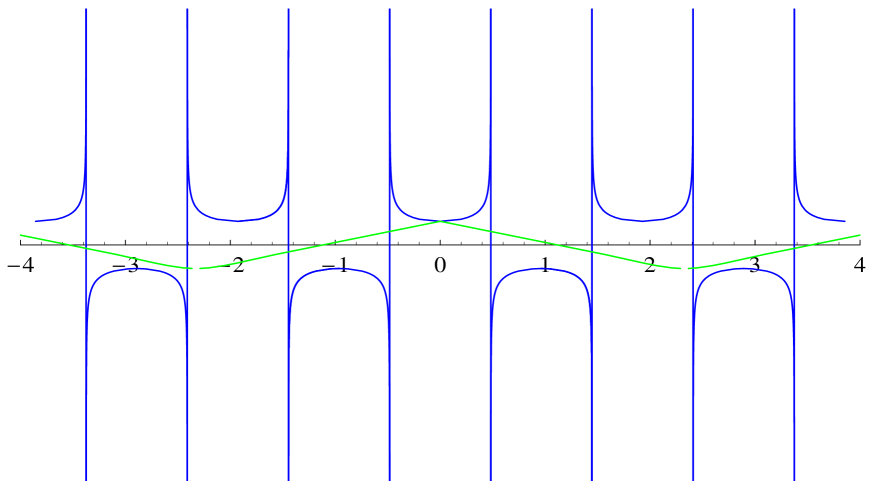
Figure 2: Numerical plot of the Jacobi elliptic function solution for the static $S^{4}$-fuzzy funnel array and the collapsing $S^{4}$-sphere at large $r_{0}$.

We believe the same numerical agreement to hold for finite $r_{0}$. However, since the asymptotics of (3.53) for large $r$ at finite $r_{0}$ were not well available with our mathematical software, we cannot confirm this.

So far we have considered the time of collapse where $r=0$ ( or the distance to blow-up in the spatial case ), but we can also consider $t$ as a function of $r$ for any finite $r$ in terms of the Appell function (3.47). The inverse expression of $r$ in terms of $t$, and more generally the complex variable $u_{1}=\sigma-it$, is contained in (4.12) and the constraint (4.15).

4.3 Solution of the problem in terms of the $u_{2}$ variable and large-small duality

We have seen that inverting the integrals (3.23) and (3.16) requires the definition of a complex variable $u_{1}=\sigma_{1}-it_{1}$ whose real and imaginary parts are related to the space and time variables. In addition we have to introduce the second holomorphic differential, so that there are $2$ complex variables $u_{1},u_{2}$. These variables are defined in terms of integrals and thus are subject to identifications by the period lattice $\cal L$ of integrals around the $a$ and $b$-cycles of the genus $2$ Riemann surface, $\Sigma_{2}$. They live on ${\mathbb{C}}^{2}/{\cal L}$, the Jacobian of $\Sigma_{2}$. Introduction of a second point $x_{2}$ on the Riemann surface relates our problem to the standard Jacobi inversion problem. The constraint $x_{2}=1$ restricts to a subvariety of the Jacobian. So far the constraint (4.15) has been viewed as determining $u_{2}$ in terms of $u_{1}$. This allowed us to describe $x_{1}$ as a function of $u_{1}$ in the neighbourhood of $x_{1}=1$ and also to get new formulae for the time of collapse/distance to blow-up which have been checked numerically against evaluation of the integrals using Appell functions. However, it is also of interest to consider using the constraint to solve $u_{1}$ in terms of $u_{2}$ and hence describe $x_{1}$ as a function of $u_{2}$. The reason for this is that the automorphisms of the Riemann surface allow us to relate the large $r$ (equivalently large $x_{1}$) behaviour of the spatial problem described in terms of the $u_{1}$ variable, to the small $r$ (equivalently small $x_{1}$) behaviour of the time dependent problem described in terms of the $u_{2}$ variable and vice versa. The relation is simpler in the large $r_{0}$ limit, hence we describe this first and then we return to the case of finite $r_{0}$.

The use of the $u_{2}$ variable is natural if we introduce another Lagrangian of the type (B.1), with $\alpha=2$. The original Lagrangian of interest with $\alpha=0$ and the $\alpha=2$ Lagrangian are coupled in the Jacobi Inversion problem (4) as well as the constrained version of the Jacobi Inversion problem (4) obtained by setting $x_{2}=1$. Just as $u_{1}$ is the complexified variable for the first Lagrangian, $u_{2}$ is the complexified space-time variable for the second Lagrangian. It will be convenient, for the following discussion, to define the relation between the second set of space-time variables $t_{2},\sigma_{2}$ and the complex variable $u_{2}$ as $u_{2}=-\sigma_{2}+it_{2}$.

We have also seen that the automorphism $U_{1}$ of section 3.4 maps $du_{1}$ to $-idu_{2}$ as in (3.45), hence takes the time dependent problem for the first kind of Lagrangian to the static one for the second mapping zeroes of a given periodicity to poles of the same periodicity. We will check this by investigating what happens to $u_{2}$ when we follow the collapse of $x_{1}$ down to zero along imaginary $u_{2}$, or the blow-up of $x_{1}$ to infinity along real $u_{2}$. It is clear from the integrals in (4) (and the series expansion (4.16)) that when $x_{1}$ decreases from 1 to 0, both $u_{1}$ and $u_{2}$ are imaginary and when $x_{1}$ increases from 1 to infinity, both are real.

Solving for $u_{2}$, the second of the equations (4.7) will give

$$u_{2}=\frac{u_{+}+u_{-}}{2\sqrt{(1-\alpha)(1-\beta)}}$$ (4.37)

and by following the steps leading to (4.27) and (4.2) we arrive at

$$u_{2}=-2^{-3/4}\cos{\frac{\pi}{8}}(A^{\prime}+iB^{\prime})K(k_{+})\;.$$ (4.38)

Here we used $tan{\frac{\pi}{8}}=\sqrt{2}-1$. The $A^{\prime}$s and $B^{\prime}$s are given by

$$\displaystyle A^{\prime}_{1}=2m_{+}+2n_{-}+2m_{-}-6n_{+}+2\;, A^{\prime}_{2}=2n_{+}-2n_{-}$$

$$B^{\prime}_{1}=2+6m_{-}+2n_{-}-2m_{+}+2n_{+}\;, B^{\prime}_{2}=2m_{+}-2m_{-}\;.$$ (4.39)

Notice by comparing (4.2) and (4.3), that $A_{1}^{\prime}=A_{1},B_{1}^{\prime}=-B_{1}$ and $A_{2}^{\prime}=-A_{2},B_{2}^{\prime}=B_{2}$. By choosing $m_{-}=-1$, $m_{+}=n_{-}=n_{+}=0$ we get

$$\displaystyle u_{2} = 2i(2-\sqrt{2})\cos{\frac{\pi}{8}}2^{-3/4}K\left(k_{+}\right)$$ (4.40)

$$\simeq i\;0.9639..\;,$$

which is exactly the same as in (4.34) in agreement with what we expect from the automorphism. Similarly for the real case

$$\displaystyle u_{2} = -2\sqrt{2}\cos{\frac{\pi}{8}}2^{-3/4}K\left(k_{+}\right)$$ (4.41)

$$\simeq -2.3271..\;.$$

With the definition $u_{2}=-\sigma_{2}+it_{2}$ we see that we are getting the expected positive time of collapse in terms of the alternative time-variable and the expected positive distance to blow-up with the alternative spatial variable. The matching of the $A^{\prime}$ and $B^{\prime}$ with $A$ and $B$ guarantees that $x_{1}$, expressed as a function of $u_{2}$, will have zeroes along the imaginary axis at odd integer multiples of a basic time of collapse and poles along the real axis at odd integer multiples of a basic distance to blow-up. The time of collapse for $u_{2}$ is the same as the distance to blow-up for $u_{1}$ and the distance to blow-up for $u_{2}$ is the same as the time of collapse for $u_{1}$. This gives a precise map between the behaviour at zero and the behaviour at infinity of the radius of the fuzzy sphere, generalising the relations that were found for the case of the fuzzy $2$-sphere. This relation is expected from the automorphism $U_{1}$ for large $r_{0}$ described in section 3, which maps $u_{1}$ to $-iu_{2}$ (3.45). This precise large-small relation for space and time-dependent fuzzy spheres is physically interesting. The physics of the large $r$ limit is very well understood because it corresponds to the D-strings blowing up into a D5-brane. The physics of the small $r$ limit appears mysterious because it involves sub-stringy distances. We have shown that the two regions are closely related through the underlying Riemann surface which unifies the space and time aspects of the problem.

4.3.1 Large-small duality at finite $r_{0}$

We saw in the discussion above that the spatial problem of the fuzzy $S^{4}$ evolving from a minimum size at $r_{0}$ to infinity can be related to the time-dependent problem of the fuzzy sphere collapsing from $r_{0}$ to zero. This large-small relation involves a map between the $u_{1}$ description and the $u_{2}$ description of the problem and uses a simplification which is valid at large $r_{0}$. There continues to be a large-small duality at finite $r_{0}$, but it is slightly more involved than the one at large $r_{0}$. The difference is due to the nature of the automorphisms of the Riemann surface at finite $r_{0}$ and in the large $r_{0}$ limit, which were described in detail in section 3.4. Indeed, the discussion above used the automorphism $U_{1}$ in a crucial way.

To describe the duality at finite $r_{0}$, it is useful to think of a problem similar to the one we considered above, by choosing a different basepoint in (4), i.e. $x_{0}=-iR_{1}^{2}$

$$\displaystyle\int_{-iR_{1}^{2}}^{\tilde{x}_{1}}\frac{dx}{y} = \tilde{u}_{1}$$

$$\int_{-iR_{1}^{2}}^{\tilde{x}_{1}}\frac{xdx}{y} = \tilde{u}_{2}\;.$$ (4.42)

The upper limit is chosen, in the first instance, to vary along the negative imaginary axis up to zero. A second problem is to consider $\tilde{x}_{1}$ extending along the negative imaginary axis down to infinity.

Applying the automorphism $T_{1}$ of (3.37) to the first line of (4) we have

$$\displaystyle u_{1}(x_{1}) = \int_{1}^{x_{1}}{dx\over y}$$

$$= {e^{i\pi\over 4}\over R_{1}}\int_{-iR_{1}^{2}}^{\tilde{x}_{1}=-{iR_{1}^{2}\over x}}{XdX\over Y}$$

$$= {e^{i\pi\over 4}\over R_{1}}\tilde{u}_{2}\left(\tilde{x}_{1}=-{iR_{1}^{2}\over x}\right)\;.$$

Similarly we have

$$u_{2}(x_{1})=R_{1}e^{\frac{i\pi}{4}}\tilde{u}_{1}\left(\tilde{x}_{1}=-{iR_{1}^{2}\over x}\right)\;.$$ (4.43)

As we saw earlier in this section, the solution to (4) can be described in terms of either the $u_{1}$ or the $u_{2}$ variable. Likewise the inversion of (4.3.1) can be expressed in terms of either $\tilde{u}_{1}$ or $\tilde{u}_{2}$. The action of the automorphism $T_{1}$ described above implies that the solution of the spatial problem (4) where $x_{1}$ evolves from $1$ to infinity along the real axis, when given in terms of the real part of the $u_{1}$ variable, maps to the evolution of $\tilde{x}_{1}$ from $-iR_{1}^{2}$ along the imaginary axis to zero, as described by the $\tilde{u}_{2}$ variable. Similarly the time-dependent problem of $x_{1}$ evolving from $1$ to zero when described in terms of the imaginary part of the $u_{1}$ variable, maps to the evolution of $\tilde{x}_{1}$ along the imaginary axis from $-iR_{1}^{2}$ to infinity, as described by the $\tilde{u}_{2}$ variable. This shows that there continues to be a large-small duality at finite $r_{0}$, but it relates the original problem with real $x$ to a problem with imaginary $x$.

5 Space and Time dependent Fuzzy-$S^{6}$

Here we will briefly talk about the nature of the solution in the case of the $D1\perp D7$ intersection, discussed by [3], which involves the fuzzy-$S^{6}$. Starting from the D-string theory point of view, we will now have seven transverse scalar fields, given by the ansatz

$$\Phi^{i}(\sigma,\tau)=\pm\hat{R}(\sigma,\tau)G^{i},\qquad i=1,\ldots 7\;,$$ (5.1)

where the $G^{i}$’s are given by the action of the $SO(7)$ $\Gamma^{i}$’s on the symmetric and traceless $n$-fold tensor product of the basic spinor $V$, the dimension of which is related to $n$ by [24]

$$N=\frac{(n+1)(n+2)(n+3)^{2}(n+4)(n+5)}{360}\;.$$ (5.2)

Again, the radial profile and the fuzzy-$S^{6}$ physical radius are related by

$$R_{ph}(\sigma,\tau)=\sqrt{c}\lambda\hat{R}(\sigma,\tau)\;,$$ (5.3)

with $c$ the quadratic Casimir $G^{i}G^{i}=c\mathbf{1}_{N}=n(n+6)\mathbf{1}_{N\times N}$. The time-dependent generalisation for the leading $1/N$ action of [3] can be written in dimensionless variables, which are once more defined as in (2.10),

$$S_{1}=-N\;T_{1}\int d^{2}\sigma\sqrt{1+r^{\prime 2}-\dot{r}^{2}}\left(1+r^{4}\right)^{3/2}\;.$$ (5.4)

In a manner identical to the discussion in section 3, the equations of motion can be given in a Lorentz-invariant expression

$$\partial_{\mu}\partial^{\mu}r+(\partial_{\mu}\partial^{\mu}r)\;(\partial_{\nu}r)\;(\partial^{\nu}r)-(\partial_{\mu}\partial^{\nu}r)\;(\partial_{\nu}r)\;(\partial^{\mu}r)=6\;r^{3}\left(\frac{1+(\partial_{\mu}r)\;(\partial^{\mu}r)}{1+r^{4}}\right)\;.$$ (5.5)

At this point it is natural to propose that the form of the action and the equations of motion will generalise in a nice way for any fuzzy-$S^{2k}$ sphere

$$S_{1}=-T_{1}\int d\sigma^{2}STr\sqrt{\left(1+r^{\prime 2}-\dot{r}^{2}\right)\left(1+r^{4}\right)^{k}}\;,$$ (5.6)

with the large-$N$ equations of motion

$$\partial_{\mu}\partial^{\mu}r+(\partial_{\mu}\partial^{\mu}r)\;(\partial_{\nu}r)\;(\partial^{\nu}r)-(\partial_{\mu}\partial^{\nu}r)\;(\partial_{\nu}r)\;(\partial^{\mu}r)=2k\;r^{3}\left(\frac{1+(\partial_{\mu}r)\;(\partial^{\mu}r)}{1+r^{4}}\right)\;.$$ (5.7)

As we saw in the previous cases, there will be a curve related to the blow-up of the funnel, derived by the conservation of pressure if we restrict to static configurations and also to the corresponding collapse of a $D6$-brane by conservation of energy if we completely drop the space variable. We find that the curve determining the solutions is

$$s^{2}=(r^{4}-r_{0}^{4})(r^{4}-r_{1}^{4})(r^{4}-r_{2}^{4})\;,$$ (5.8)

which is of genus 5 and where a factor of $(1+r_{0}^{4})$ has been absorbed in the definition of $s$. The roots are given by

$$\displaystyle(1+r_{0}^{4}) = u_{0}^{4}$$

$$(1+r_{1}^{4}) = u_{0}^{4}\eta$$

$$(1+r_{2}^{4}) = u_{0}^{4}\eta^{2}\;,$$ (5.9)

with $\eta=\exp{2i\pi\over 3}$.

• Automorphism at large $r_{0}$ :
  At large $r_{0}$, we have $r_{1}^{4}=r_{0}^{4}\eta$ and $r_{2}^{4}=r_{0}^{4}\eta^{2}$. Then there exists an automorphism

  $$\displaystyle R = {r_{0}^{2}\over r}$$

  $$S^{2} = -{s^{2}r_{0}^{12}\over r^{12}}\;.$$

  It is convenient to define ${\tilde{r}}={r\over r_{0}}$, and ${\tilde{s}}^{2}=s^{2}r_{0}^{12}$. In these variables

  $$\displaystyle{\tilde{r}}\rightarrow{1\over{\tilde{r}}}$$

  $$\tilde{s}\rightarrow{i\tilde{s}\over{\tilde{r}}^{6}}$$

  and the action on the holomorphic differentials is

  $$\displaystyle\omega_{1} \rightarrow i\omega_{5}$$

  $$\omega_{2} \rightarrow i\omega_{4}$$

  $$\omega_{3} \rightarrow i\omega_{3}$$

  $$\omega_{4} \rightarrow i\omega_{2}$$

  $$\omega_{5} \rightarrow i\omega_{1}\;.$$

• Automorphism at $r_{0}=0$ :
  Now we have

  $$s^{2}=r^{4}(r^{4}-r_{1}^{4})(r^{4}-r_{2}^{4})$$ (5.10)

  and there is an automorphism

  $$\displaystyle R = {r_{1}r_{2}\over r}$$

  $$S^{2} = {s^{2}(r_{1}r_{2})^{8}\over r^{16}}\;.$$

  In this limit $r_{1}^{4}=(\eta-1)$ and $r_{2}^{4}=(\eta^{2}-1)$, so in the formulae above we can write $r_{1}^{4}r_{2}^{4}=3$.

• Symmetry at finite $r_{0}$ :
  It is useful to write the curve in terms of a variable $u$ defined by $u^{4}=(1+r^{4})$ and to write $u_{0}^{4}=1+r_{0}^{4}$. Then we have

  $$s^{2}=(u^{4}-u_{0}^{4})(u^{4}-u_{0}^{4}\eta)(u^{4}-u_{0}^{4}\eta^{2})\;.$$ (5.11)

  A symmetry is $v={u_{0}^{2}\over u}$, ${\tilde{s}}^{2}=-{s^{2}u_{0}^{12}\over u^{12}}$. Expressing the symmetry in the $r,s$ variables, we have $R,S$ obeying the same equation (5.8) with

  $$\displaystyle(1+R^{4}) = {(1+r_{0}^{4})^{2}\over(1+r^{4})}$$

  $$S^{2} = -{s^{2}(1+r_{0}^{4})^{3}\over(1+r^{4})^{3}}\;.$$

  This reduces to the $R={r_{0}^{2}\over r}$ for $r>>1$, $R>>1$, $r_{0}>>1$. Unfortunately $R$ is not a rational function of $r$, but an algebraic function of $r$ involving fourth roots, hence it is not a holomorphic or meromorphic function. Hence it is not possible to use this symmetry to map the holomorphic differentials of the genus $5$ curve to those on genus $1$ curves. We can still make the change of variables $x=r^{2}$ to get a reduction down to genus $3$, but we have not been able to reduce this any further.

Since we cannot reduce the curve down to a product of genus one curves, we cannot relate the problem of inverting the hyper-elliptic integral to elliptic functions. We can nevertheless relate it to the Jacobi inversion problem at genus $3$. We consider variables $u_{1},u_{2},u_{3}$ defined as

$$\displaystyle\int_{1}^{x_{1}}\omega_{1}+\int_{1}^{x_{2}}\omega_{1}+\int_{1}^{x_{3}}\omega_{1} \equiv u_{1}$$

$$\int_{1}^{x_{1}}\omega_{2}+\int_{1}^{x_{2}}\omega_{2}+\int_{1}^{x_{3}}\omega_{2} \equiv u_{2}$$

$$\int_{1}^{x_{1}}\omega_{3}+\int_{1}^{x_{2}}\omega_{3}+\int_{1}^{x_{3}}\omega_{3} \equiv u_{3}\;.$$

The variables $u_{1},u_{2},u_{3}$ live on the Jacobian of the genus three curve, which is a complex torus of the form ${\mathbb{C}}^{3}/{\cal L}$. The integrands appearing above live naturally on a Riemann surface which is a cover of the complex plane, branched at 8 points. The lattice $\cal L$ arises from doing the integrals around the $a$ and $b$-cycles of the Riemann surface. The equations (5) can be inverted to express

$$\displaystyle x_{1} = x_{1}(u_{1},u_{2},u_{3})$$

$$x_{2} = x_{2}(u_{1},u_{2},u_{3})$$

$$x_{3} = x_{3}(u_{1},u_{2},u_{3})\;,$$

where $x_{i}(u_{1},u_{2},u_{3})$ can be given in terms of genus three theta functions, or equivalently in terms of hyper-elliptic Kleinian functions [25]. The system (5) simplifies if we set $x_{2}=x_{3}=1$. These simplified equations define a sub-variety of the Jacobian which is isomorphic to the genus $3$ Riemann surface we started with [20]. The constraints $x_{2}=x_{3}=1$ can be used to solve, at least locally near $x_{1}=1$, for $u_{2},u_{3}$ in terms of $u_{1}$. Then we can write $x_{1}(u_{1},u_{2},u_{3})$ as $x_{1}(u_{1})$. This program was carried out explicitly in section 3, where the higher genus theta functions degenerated into expressions in terms of ordinary elliptic functions thanks to the reduction of the genus three curve we started with, to a product of genus one curves. For completeness, we give a short review of the solution to the Jacobi Inversion problem in terms of higher genus $\vartheta$ functions and the related Kleinian $\sigma$-function.

5.1 Jacobi inversion problem and $\vartheta$ functions

The general Jacobi inversion problem can be formulated as follows [15, 16, 25]. For any hyper-elliptic curve $\Sigma$ of genus $g$, realised as a 2-sheeted cover over a Riemann sphere

$$y^{2}=\sum_{i=0}^{2g+2}\lambda_{i}x^{i}=\prod_{i=1}^{g+1}(x-a_{i})\prod_{i=1}^{g+1}(x-c_{i})\;,$$ (5.12)

with $a$’s and $c$’s being the branch points, between which we stretch the cuts, the system of integral equations

$$\displaystyle\int_{a_{1}}^{x_{1}}\omega_{1}+\ldots+\int_{a_{g}}^{x_{g}}\omega_{1} \equiv u_{1}$$

$$\vdots \vdots$$

$$\int_{a_{1}}^{x_{1}}\omega_{g}+\ldots+\int_{a_{g}}^{x_{g}}\omega_{g} \equiv u_{g}\;,$$

describes the invertible Abel map, $\mathit{U}:\Sigma^{g}/S_{g}\longrightarrow\textrm{Jac}(\Sigma)$, taking $g$ symmetric points from the Riemann surface to the Jacobian of $\Sigma$. The latter is just $\mathbb{C}^{g}/\mathcal{L}$, where $\mathcal{L}=2\zeta\oplus 2\zeta^{\prime}$ is the lattice that is generated by the non-degenerate periods of the holomorphic differentials, or differentials of the first kind, defined on the surface

$$2\zeta=\oint_{A_{k}}\omega_{l}\quad\textrm{and}\quad 2\zeta^{\prime}={\oint_{B_{k}}\omega_{l}}\;,$$ (5.13)

with

$$\omega_{i}=\frac{x^{i-1}dx}{y}\;,\qquad i=1,\ldots,g\;.$$ (5.14)

The period matrix is the $g\times g$ matrix given by $\tau=\zeta^{-1}\zeta^{\prime}$ and belongs to the Siegel upper halfspace of degree $g$, having positive imaginary part and being symmetric. There is also a set of canonical meromorphic differentials, or differentials of the second kind, naturally defined on the Riemann surface

$$\xi_{j}=\sum_{k=j}^{2g+1-j}(k+1-j)\lambda_{k+1-j}\frac{x^{k}dx}{4y}\;,\qquad j=1,\ldots,g\;,$$ (5.15)

the periods of which are

$$2\eta=-\oint_{A_{k}}\xi_{l}\quad\textrm{and}\quad 2\eta^{\prime}=-\oint_{B_{k}}\xi_{l}\;.$$ (5.16)

Now consider $\textbf{\emph{m}},\textbf{\emph{m}}^{\prime}\in\mathbb{Z}^{g}$ two arbitrary vectors and define the periods

$$\Omega(\textbf{\emph{m}},{\textbf{\emph{m}}}^{{}^{\prime}})=2\zeta\textbf{\emph{m}}+2\zeta^{\prime}\textbf{\emph{m}}^{\prime}\quad\textrm{and}\quad E(\textbf{\emph{m}},{\textbf{\emph{m}}}^{\prime})=2\eta\textbf{\emph{m}}+2\eta^{\prime}\textbf{\emph{m}}^{\prime}\;.$$ (5.17)

We can define the fundamental Kleinian $\sigma$-function in terms of higher genus Riemann $\vartheta$-functions

$$\sigma(\textbf{\emph{u}})=Ce^{\emph{{u}}^{T}\kappa\emph{{u}}}\vartheta((2\omega^{-1})\emph{{u}}-\textbf{K}_{a}|\tau)\;,$$ (5.18)

where $C$ is a constant, $\kappa=(2\zeta)^{-1}\eta$ and $\textbf{K}_{a}$ is the vector of Riemann constants with base point $a$, given by the Riemann vanishing theorem

$$\textbf{K}_{a}=\sum_{k=1}^{g}\int_{a}^{a_{i}}d\textbf{v}\;,$$ (5.19)

with $d\textbf{v}=(2\zeta^{-1})(\textbf{\emph{$\omega_{1}$}},\ldots,\textbf{\emph{$\omega_{g}$}})^{T}$ being the set of normalised canonical holomorphic differentials. Furthermore, the genus-g Riemann $\vartheta$-function with half-integer characteristics $[\varepsilon]=\left[\begin{array}[]{c}\varepsilon^{\prime}\\ \varepsilon\\ \end{array}\right]=\left[\begin{array}[]{ccc}\varepsilon_{1}^{\prime}&\ldots&\varepsilon_{g}^{\prime}\\ \varepsilon_{1}&\ldots&\varepsilon_{g}\end{array}\right]\in\mathbb{C}^{2g}$ is defined as

$$\vartheta[\varepsilon](\textbf{\emph{v}}|\tau)=\sum_{\textbf{\emph{m}}\in\mathbb{Z}^{g}}\exp\;\pi i\left\{(\textbf{\emph{m}}+\varepsilon^{\prime})^{T}\tau\;(\textbf{\emph{m}}+\varepsilon^{\prime})+2(\textbf{\emph{v}}+\varepsilon)^{T}(\textbf{\emph{m}}+\varepsilon^{\prime})\right\}\;.$$ (5.20)

The general pre-image of the Abel map can be given in a simple algebraic form as the roots of a polynomial in $x$, given by

$$\mathbf{P}(x;\textbf{\emph{u}})=x^{g}-x^{g-1}\wp_{g,g}(\textbf{\emph{u}})-x^{g-2}\wp_{g,g-1}(\textbf{\emph{u}})-\ldots-\wp_{g,1}(\textbf{\emph{u}})\;.$$ (5.21)

Here $\textbf{\emph{u}}=(u_{1},\ldots,u_{g})^{T}$ and the $\wp$’s are higher genus versions of the standard Weierstrass elliptic $\wp$-functions, which are defined as the logarithmic derivatives of the fundamental hyper-elliptic $\sigma$-functions

$$\wp_{ij}(\textbf{\emph{u}})=-\frac{\partial^{2}\ln\sigma(\textbf{\emph{u}})}{\partial u_{i}\partial u_{j}}\;,\quad\wp_{ijk}(\textbf{\emph{u}})=-\frac{\partial^{3}\ln\sigma(\textbf{\emph{u}})}{\partial u_{i}\partial u_{j}\partial u_{k}}\;,\ldots\;,\quad i,j,k,\ldots\;=1,\ldots,g$$ (5.22)

and have the nice periodicity properties

$$\wp_{ij}(\textbf{\emph{u}}+\Omega({\textbf{\emph{m}},\emph{{m}}}^{\prime}))=\wp_{ij}(\textbf{\emph{u}})\;,\quad i,j=1,\ldots,g\;.$$ (5.23)

We can make use of all this technology and give at least an implicit solution for the $S^{6}$ at the stage where we have been able to reduce the problem from one of genus-5, to one of genus-3. By equating the general polynomial with roots $x_{1},x_{2},x_{3}$ to the polynomial with $\wp$-coefficients, we get

$$\displaystyle x_{1}+x_{2}+x_{3}=\wp_{33}(u_{1},u_{2},u_{3})$$

$$x_{1}x_{2}x_{3}=\wp_{23}(u_{1},u_{2},u_{3})$$

$$x_{1}x_{2}+x_{2}x_{3}+x_{3}x_{1}=-\wp_{13}(u_{1},u_{2},u_{3})\;.$$ (5.24)

As we have already mentioned, we can fix two of the three points to be $x_{2}=x_{3}=1$, to get

$$\displaystyle x_{1}+2=\wp_{33}(u_{1},u_{2},u_{3})$$

$$x_{1}=\wp_{23}(u_{1},u_{2},u_{3})$$

$$2x_{1}+2=-\wp_{13}(u_{1},u_{2},u_{3})\;.$$ (5.25)

This implies two transcendental constraints which can be used to get a solution for $x_{1}$, in terms of the $\wp$’s as functions of $u_{1}$.

6 Summary and Outlook

The space and time dependence of fuzzy spheres $S^{2}$, $S^{4}$ and $S^{6}$ are governed by equations which follow from the DBI action of D-branes. These fuzzy spheres can arise as bound states of D0 with D2, D4 or D6 on the one hand, or as cross-sections of fuzzy funnels formed by D1 expanding into D3, D5 or D7 on the other. The purely time-dependent process has the simplest realisation as the collapsing-expanding $D0-D2p$-brane, although it also arises as a time dependent process for the $D1-D(2p+1)$ equations with no variation along the spatial $D1$-direction. The first order equations of motion are closely related to some Riemann surfaces and the infinitesimal time elapsed or the infinitesimal distance along the D1, are given by a holomorphic differential on these surfaces. We have given descriptions of the solutions in terms of elliptic functions or their higher genus generalisations. We showed that the space and time processes exhibit some very interesting large-small dualities closely related to the geometry of the Riemann surfaces.

In the case of $S^{2}$, the Riemann surface has genus one and the duality is related to properties of Jacobi elliptic functions known as “complex multiplication formulae” [9]. The genus $1$ Riemann surface that arises here has automorphisms, holomorphic maps to itself, which are responsible for these properties. We observed that the large-small duality is also directly related to a transformation property of the second order differential equations.

In the case of $S^{4}$ we derived formulae for the distance $\sigma(r)$ along the D1-brane as a function of the radius of the funnel’s fuzzy sphere cross-section and the time elapsed $t(r)$ as a function of the radius. These formulae were expressed in terms of special functions such as Appell and hypergeometric functions. It was useful to combine space and time into a complex variable $u_{1}=\sigma-it$ which was related to a genus three Riemann surface, having a number of automorphisms. These automorphisms were used to eventually relate the problem to a product of two genus one Riemann surfaces. After introducing a second complex variable $u_{2}$, the problem of inverting the integrals to get a formula for the radius as a function of the complexified space-time variable $u_{1}$ was related to a classical problem in Riemann surfaces, the Jacobi Inversion problem. This can be solved, in general, using higher genus theta functions. The relation to a product of genus one surfaces in the case at hand, means that the inversion problem can be expressed in terms of the standard elliptic integrals. This allowed us to give a solution of the inversion problem in terms of standard Jacobi elliptic functions. The solution involves a constraint in terms of elliptic functions, which can be used to solve $u_{2}$ in terms $u_{1}$, or vice versa. This approach yields a new construction of $r(u_{1})$ as a series around $r=r_{0}$, which agrees with a direct series inversion of the Appell function. It also gives new formulae for the time of collapse and distance to blow-up in terms of sums of complete elliptic integrals, which were checked numerically to agree with the formulae in terms of hypergeometric functions.

The automorphism which allows a reduction of the problem to one involving genus one surfaces also relates the large $r$ behaviour of the spatial (time-dependent) solutions to the small $r$ behaviour of the time-dependent (spatial) problem. The introduction of the extra variable $u_{2}$, required to make a connection to the Jacobi inversion problem, also enters the description of this large-small duality.

Our discussion in the $S^{6}$ case was less complete, but a lot of the structure uncovered above continues to apply. The integrals giving $t(r)$ or $\sigma(r)$ are integrals of a holomorphic differential on a genus $5$ Riemann surface. A simple $R=r^{2}$ transformation maps it to a holomorphic differential on a genus $3$ curve. The inversion problem of expressing $r$ in terms of $u_{1}=\sigma-it$ can be related to the Jacobi inversion problem and a solution in terms of higher genus theta functions is outlined. We did not find any automorphisms of the genus $3$ Riemann surface which would relate the problem to one involving holomorphic differentials on a genus $1$ curve. There do continue to exist symmetry transformations of the curve but they are no longer holomorphic in terms of the $(r,s)$ variables.

It will be interesting to consider the full CFT description of these funnels. Some steps towards the full CFT description of these systems has been made [26]. There should be a boundary state describing the spatial configuration of a D1-branes forming a funnel which blows up into a D3-brane. One could start with the CFT of the multiple D1-branes and consider a boundary perturbation describing the funnel which opens into a D3. Alternatively we could start with a CFT for the D3 and introduce boundary perturbations corresponding to the magnetic field strength and the transverse scalar excited on the brane, which describe the D1-spike. In either case the boundary perturbation will involve the elliptic functions which appeared in section $2$. Similarly the boundary perturbation for the fuzzy $S^{4}$ case would involve elliptic functions associated with a pair of genus $1$ Riemann surfaces, of the type described in section 4. One such boundary state corresponds to the purely time-dependent solution and another to the purely space-dependent solution. If the large-small duality of the DBI action continues to hold in the CFT context, this would give a remarkable relation between the zero radius limit of time-dependent brane collapse and the well-understood blow-up of a D1-brane funnel into a higher dimensional brane. Analytic continuations from Minkowski to Euclidean space in the context of boundary states have proved useful in studies of the rolling tachyon [27]. We expect similar applications of the analytic structures described here.

A complementary way to approach these dualities is to consider the supergravity description. The time dependent system of a collapsing D0-D2-brane, for example, should correspond to a time-dependent supergravity background, when the backreaction of spacetime to the stress tensor of the D0-D2 system is taken into account. A Wick rotation of this background can convert the time-like co-ordinate $t$ to a space-like co-ordinate. Similarly the spatial funnel of a D1-D3 system has a supergravity description with an $S^{2}$ having a size that depends on the distance along the direction of the D-string. The Wick rotated D2-background should be related by a large-small duality to the D1-D3 system. This is a sort of generalisation of $S^{1}$ T-duality to $S^{2}$. Similarly, the $D0-D4$ system is related to the $D1\perp D5$. The Jacobi Inversion problem which underlies our solutions has already arisen in the context of general relativity [28]. It will be interesting to see if this type of GR application of the Jacobi Inversion also arises in the spacetime solutions corresponding to our brane configurations. Another perspective on the geometry of these configurations , including the boosted ones in the Appendix A.1, and on the relations to $S$-branes, should be provided by considering the induced metric on the brane as for example in [29].

Generalisation of this discussion to funnels of $\mathbb{CP}^{2}$ and other cross-sections, as well as to funnels made of dyonic strings will be interesting. The study of finite $n$ corrections as in [4] is another interesting avenue.

Studying fluctuations around the solutions considered is likely to involve equations where the elliptic functions and their higher genus generalisations appear as potentials in Dirac or Klein-Gordon type equations for the fluctuations. Schrödinger equations with such potentials are well studied in the literature of integrable models [30]. It will be interesting to see if such integrable models have a role in the analysis of fluctuations.

Finally, the genus $3$ curve for the $S^{4}$ was very special. It is a related by the $R=r^{2}$ map to a product of genus $1$ and a genus $2$ curve. The resulting genus $2$ curve itself has a Jacobian which is related to $K3$ Kummer surfaces and factorises into a product of genus one curves [16]. Special $K3$’s and complex multiplication also appear in the attractor mechanism [31, 32]. Whether the appearances of special $K3$’s in these two very different ways in string theory are related is an intriguing question.

Acknowledgements: We thank Robert de Mello Koch, Jose Figueroa-O’Farrill, Pei Ming Ho, Simon McNamara, Bill Spence, Radu Tatar, Steve Thomas, Nick Toumbas, Gabriele Travaglini and John Ward for discussions. The work of SR is supported by a PPARC Advanced Fellowship. CP would like to acknowledge a QMUL Research Studentship. This work was in part supported by the EC Marie Curie Research Training Network MRTN-CT-2004-512194.

Appendix A Further aspects of space-time dependence of $S^{2}$ funnel

A.1 Lorentz Invariance of the BPS condition

We will study the supersymmetry of the space and time-dependent system considered in section 2, in order to obtain a Lorentz invariant BPS condition. The vanishing of the variation of the gaugino on the world-volume of the intersection will require that [1]

$$\delta\chi=\Gamma^{\mu\nu}F_{\mu\nu}\;\epsilon=0\;,$$ (A.1)

where $\mu,\nu$ spacetime indices, with

$$F_{ab}=0\qquad F_{ai}=D_{a}\Phi_{i}\qquad F_{ij}=i[\Phi^{i},\Phi^{j}]\qquad\textrm{and}\qquad a=\sigma,\tau\quad,\quad i=1,2,3\;.$$ (A.2)

Here the spinor $\epsilon$ already satisfies the D-string projection $\Gamma^{\tau\sigma}\epsilon=\epsilon$ and multiply indexed $\Gamma$’s denote their normalised, fully antisymmetric product, e.g. $\Gamma^{\mu\nu}=\frac{1}{2}[\Gamma^{\mu},\Gamma^{\nu}]$. Then

$$\left(i\Gamma^{jk}[\Phi^{j},\Phi^{k}]+2\Gamma^{ai}D_{a}\Phi^{i}\right)\epsilon=0\;.$$ (A.3)

We will consider the conjugate spinor

$$\overline{\delta\chi}=\delta\chi^{{\dagger}}\;\Gamma^{0}$$ (A.4)

and construct the invariant quantity

$$\delta\chi^{\dagger}\;\Gamma^{0}\;\delta\chi=0\;,$$ (A.5)

where our conventions for the $\Gamma$-matrices are

$$(\Gamma^{0})^{2}=-1\>,\quad(\Gamma^{i})^{2}=1\quad\textrm{and}\quad(\Gamma^{\mu})^{\dagger}=\Gamma^{0}\Gamma^{\mu}\Gamma^{0}\;,\quad(\Gamma^{\mu\nu})^{\dagger}=\Gamma^{0}\Gamma^{\mu\nu}\Gamma^{0}\;.$$ (A.6)

Then (A.5) becomes

$$\epsilon^{\dagger}\left(-i\;(\Gamma^{\ell m})^{\dagger}[\Phi^{\ell},\Phi^{m}]+2(\Gamma^{bi})^{\dagger}D_{b}\Phi^{i}\right)\;\Gamma^{0}\left(i\;\Gamma^{jk}[\Phi^{j},\Phi^{k}]+2\Gamma^{ai}D_{a}\Phi^{i}\right)\epsilon=0\;.$$ (A.7)

This will give three kinds of terms: Quadratic terms in derivatives, a quadratic term in commutators of $\Phi^{i}$ and cross-terms. The first of these will be

$$4(D_{a}\Phi^{i})(D_{b}\Phi^{j})\;\epsilon^{\dagger}(\Gamma^{0}\Gamma^{bj}\Gamma^{0})(\Gamma^{0}\Gamma^{ai})\epsilon\;.$$ (A.8)

By making use of the ansatz $\Phi^{i}=\hat{R}(\sigma,\tau)\alpha^{i}$ and by taking a trace over the gauge indices this becomes

$$4(\partial_{a}\hat{R})(\partial_{b}\hat{R})\;Tr\;(\alpha^{i}\alpha^{j})\;\epsilon^{\dagger}\left(\Gamma^{0}\frac{1}{2}\{\Gamma^{b},\Gamma^{a}\}\Gamma^{j}\Gamma^{i}+\Gamma^{0}\frac{1}{2}[\Gamma^{b},\Gamma^{a}]\Gamma^{j}\Gamma^{i}\right)\epsilon$$ (A.9)

Since $\{\Gamma^{\mu},\Gamma^{\nu}\}=2g^{\mu\nu}$, $Tr\;\alpha^{i}\alpha^{j}=\hat{c}\;\delta^{ij}$ for a constant $\hat{c}$ and the expression is symmetric in $a,b$ we get

$$12\;\hat{c}\;(\partial_{a}\hat{R})(\partial^{a}\hat{R})\left(\epsilon^{\dagger}\Gamma^{0}\epsilon\right)\;.$$ (A.10)

The product of commutators will be

$$-[\Phi^{\ell},\Phi^{m}][\Phi^{j},\Phi^{k}]\;\epsilon^{\dagger}\Gamma^{0}\Gamma^{\ell m}\Gamma^{jk}\epsilon\;,$$ (A.11)

which with the trace and the use of the ansatz becomes

$$4\hat{c}\hat{R}^{4}\;\varepsilon^{\ell mp}\varepsilon^{jkq}\delta^{pq}\;\epsilon^{\dagger}\Gamma^{0}\Gamma^{\ell m}\Gamma^{jk}\epsilon\;.$$ (A.12)

Since we are looking for a supersymmetry condition for the intersection, we want the spinor $\epsilon$ to satisfy $\Gamma^{\tau ijk}\epsilon=\varepsilon^{ijk}\epsilon$ appropriate for the $D3$-brane. Using this fact we can re-write the above as

$$-4\hat{c}\hat{R}^{4}\;(\delta^{\ell j}\delta^{mk}-\delta^{\ell k}\delta^{mj})\;\varepsilon^{\ell mn}\varepsilon^{jkn}\;\epsilon^{\dagger}\Gamma^{0}\epsilon$$ (A.13)

and end up with

$$-12\;\hat{c}(4\hat{R}^{4})\;\left(\epsilon^{\dagger}\Gamma^{0}\;\epsilon\right)\;.$$ (A.14)

Finally, the cross-terms

$$2i\left(\epsilon^{\dagger}\Gamma^{0}\Gamma^{jk}\Gamma^{ai}[\Phi^{j},\Phi^{k}](D_{a}\Phi^{i})\epsilon-\epsilon^{\dagger}\Gamma^{0}\Gamma^{ai}\Gamma^{jk}(D_{a}\Phi^{i})[\Phi^{j},\Phi^{k}]\epsilon\right)$$ (A.15)

will vanish by following the same steps, since $Tr\;\alpha^{i}\alpha^{j}\alpha^{k}\sim\varepsilon^{ijk}$ and the $\Gamma$-matrix commutator is $[\Gamma^{i},\Gamma^{jk}]=(\delta^{ij}\Gamma^{k}-\delta^{ik}\Gamma^{j})$. Collecting (A.10) and (A.14) we have

$$\epsilon^{\dagger}\;\Gamma^{0}\epsilon\left((\partial^{a}\hat{R})(\partial_{a}\hat{R})-4\;\hat{R}^{4}\right)=0\;.$$

which implies

$$(\partial^{a}\hat{R})(\partial_{a}\hat{R})-4\;\hat{R}^{4}=0$$ (A.16)

By employing dimensionless variables, the supersymmetry-preserving condition is simply

$$(\partial_{\mu}r)\;(\partial^{\mu}r)=r^{4},\qquad\mu=\sigma,\tau\;.$$ (A.17)

Thus, every configuration that satisfies (A.17) qualifies as a BPS state and therefore will be semi-classically stable. The special case ${\hat{R}}^{\prime}=2(\hat{R})^{2}$ was used in [1] and is related to Nahm’s equations.

We will briefly look at some solutions of this first-order equation. It is not hard to see that the simplest ones can be put into the form

$$\hat{R}(\sigma,\tau)=\pm\frac{1}{2}\frac{1}{\gamma(\sigma-\sigma_{\infty}+\beta t)}\;,$$ (A.18)

where $\sigma_{\infty}$ a constant, $\gamma=\frac{1}{\sqrt{1-\beta^{2}}}$ and $\beta$ another constant, which can be thought of as the ratio of the velocity of the system over the speed of light $c=1$. Then the solution at hand is nothing but a boost of the static funnel

$$\hat{R}=\pm\frac{1}{2(\sigma-\sigma_{\infty})}\;.$$ (A.19)

Moreover (A.18) will satisfy the full non-linear (2.9) and is therefore a proper solution of our space and time-dependent system. In this case we can see explicitly how this solution should also satisfy the YM equations of motion. By starting with the BPS-like relation (A.17), one gets by differentiation and algebraic manipulation

$$\partial_{\mu}\partial^{\nu}r\;(\partial_{\nu}r)(\partial^{\mu}r)=2r^{3}(\partial_{\mu}r)(\partial^{\mu}r)\;,$$ (A.20)

which if substituted in (2.12) and again with (A.17), will yield exactly $\partial_{\mu}\partial^{\mu}r=2r^{3}$, which are the YM equations. Relations between the BPS condition, the DBI and YM equations were discussed in [34]. Therefore the class of space and time-dependent supersymmetric solutions to DBI simultaneously satisfy the BPS and the YM equations. Interestingly there exist solutions to one of YM or BPS which do not solve the DBI. For example, $r_{YM}=\frac{1}{\sqrt{2(\sigma^{2}-\tau^{2})}}$ solves the YM equations but not the BPS or DBI and $r_{BPS}=\frac{1}{\sqrt{\sigma^{2}-\tau^{2}}}$ is just a solution to BPS.

The fact that we have recovered, in the context of space and time dependent transverse scalars, a boosted static solution is something that we should have expected: The expression for the Born-Infeld action is, of course, Lorentz invariant. This guarantees that its extrema, and solutions to the equations of motion, although transforming accordingly under boosts, should still be valid solutions at the new points $x^{\prime}=\Lambda^{-1}x$. The lowest energy configuration of the system is naturally the BPS one and a boost provides a generalisation that is still stable and time-dependent. A natural consequence of this is the boosted brane array, which is indeed a solution of the space and time dependent DBI equations of motion

$$r(\sigma,\tau)=\pm r_{0}\frac{1}{Cn\left(\frac{\sqrt{2}r_{0}\gamma(\sigma-\beta\tau)}{\sqrt{r_{0}^{4}+1}},\frac{1}{\sqrt{2}}\right)}$$ (A.21)

and the boosted collapsing brane

$$r(\sigma,\tau)=\pm r_{0}Cn\left(\frac{\sqrt{2}r_{0}\gamma(\tau-\beta\sigma)}{\sqrt{r_{0}^{4}+1}},\frac{1}{\sqrt{2}}\right)\;.$$ (A.22)

A.2 Chern-Simons terms and D-brane charges for D1-D3 system

We found in section 2.1 that the equations of motion for a space and time-dependent ‘funnel’ configuration have a solution both in the D1 and the D3 picture. The Chern-Simons part of the non-abelian DBI in a flat background, is not relevant in the search for the equations of motion. However, it would be a nice check to see whether the charge calculation also agrees when time dependence of the scalars is introduced, as happens for the static case. We will be assuming spherical symmetry of the solutions in what follows.

We expect to recover a coupling to a higher dimensional brane through the non-commutative, transverse scalars and the dielectric effect. This is indeed the case and one gets for the $D3$-charge of the $D1$ configuration for any time-dependent solution, at large-$N$

$$S_{cs}^{D1}=\frac{2\mu_{1}}{\lambda}\int d\tau\wedge d\sigma\;R_{ph}^{2}\left(C^{(4)}_{\sigma 123}\dot{R}_{ph}-C^{(4)}_{\tau 123}R^{\prime}_{ph}\right)\;.$$ (A.23)

The Chern-Simons part of the low energy effective D3-brane action reads

$$S_{CS}=\mu_{3}\int\;Str\;P[C^{(4)}]+\mu_{3}\int\;Str\;P[C^{(2)}]\wedge F+\mu_{3}\int\;Str\;P[C^{(0)}]\wedge F\wedge F\;.$$ (A.24)

By considering a spherical co-ordinate embedding in the static gauge, the calculation of the D3 charge will give

$$S_{CS}^{D3}=4\pi\mu_{3}\int dt\wedge dR_{D3}\;R_{D3}^{2}\left[C^{(4)}_{t123}+C^{(4)}_{9123}\lambda\dot{\Phi}\right]\;,$$ (A.25)

where $R_{D3},t$ are world-volume indices and $1,2,3$ are space-time indices.

Following [2] we will make the following identifications

• The physical radius of the fuzzy $S^{2}$ on the $D1$ side should correspond to the co-ordinate $R_{D3}$ on the world-volume of the D3

  $$R_{ph}\longleftrightarrow R_{D3}\;.$$ (A.26)

• The $\sigma$ co-ordinate on the world-volume of the $D1$ should be analogous to the transverse scalar $\Phi$ on the $D3$

  $$\sigma\longleftrightarrow\lambda\Phi\;.$$ (A.27)

• We finally assume

  $$\tau\longleftrightarrow t\;.$$ (A.28)

By thinking about the physical radius of the fuzzy sphere as a function of $\sigma$ and $t$, using the relationships (2.18) and also the fact $(2\pi\sqrt{\alpha^{\prime}})^{p^{\prime}-p}\mu^{p^{\prime}}=\mu^{p}$, we are able to write (A.25) in terms of $D1$ world-volume quantities. Everything works out nicely and one gets

$$S_{CS}^{D1}=S_{CS}^{D3}\;.$$ (A.29)

Furthermore we can make use of (A.18) to get:

$$\Phi(R_{D3},t)=\pm\left(\frac{N}{2\gamma R_{D3}}-\frac{\beta t}{\lambda}\right)$$ (A.30)

as the boosted solution on the $D3$. This can be re-written as

$$\lambda\Phi(R_{D3},t)=\gamma(\lambda\Phi_{0}(R_{D3})+\beta t^{\prime})\;,$$ (A.31)

where $t^{\prime}$ is related to $t$ by a Lorentz transformation $t^{\prime}=\gamma(t-\beta\lambda\Phi)$ and can be viewed as the time co-ordinate for an observer on the worldvolume of the boosted $D3$.

Appendix B Lagrangians for holomorphic differentials

We have seen that the space or time-dependence of the radius of the fuzzy $S^{4}$ described by the Lagrangian (3.4) is given by integrating the holomorphic differential ${dr\over s}$ on the curve $(r,s)$ given by (3.22). There are more general holomorphic differentials on the same Riemann surface, which enter on equal footing in the geometry of the Riemann surface. For the hyperelliptic curves of the type we considered, they are of the form ${r^{\alpha}dr\over s}\equiv dt_{\alpha}$, where $\alpha$ can take values from $1$ to the genus of the curve. It is natural to ask if there are Lagrangians such that the time elapsed or distance are given by the more general holomorphic differentials. This is indeed possible and the Lagrangian densities are

$$L_{\alpha}=-\sqrt{1-r^{2\alpha}({\dot{r}}^{2}+{{r^{\prime}}}^{2})}(1+r^{4})\;.$$ (B.1)

The automorphisms we discussed in section 4, can be used to relate the time evolution of interest which appears as the imaginary part of $u_{1}$, to the space evolution for $\alpha=2$. The variable $u_{2}$ discussed in section 4.2 and 4.3 are related to the $\alpha=2$ holomorphic differential of the genus three curve and hence to the $\alpha=2$ Lagrangian above.

It is also interesting to explore how the second order equations following from $L_{\alpha}$ transform under inversion of $r$. Dropping the space dependence, the equation of motion following from (B.1) is

$$\ddot{r}=-{4r^{3-2\alpha}\over{1+r^{4}}}+{{\dot{r}}^{2}\over r(1+r^{4})}\bigl{(}~{}(4-\alpha)r^{4}-\alpha~{}\bigr{)}\;.$$ (B.2)

Under a transformation $R={1\over r},\tau=t$, we get

$$\ddot{R}={4R^{3+2\alpha}\over 1+R^{4}}+{{\dot{R}}^{2}\over R(1+R^{4})}\bigl{(}~{}(\alpha+2)R^{4}+(\alpha-2)~{}\bigr{)}\;.$$ (B.3)

If we ignore, for the moment, the first term on the RHS, we see that the $\alpha=0$ equation in (B.2) maps to the $\alpha=2$ term. If we neglect the velocity dependent term on the RHS, the $\alpha=0$ maps back to $\alpha=0$.

Further consider the transformation $R={1\over r},{d\tau\over dt}=-{1\over R^{2}}$, to get

$$\ddot{R}={4R^{7+2\alpha}\over 1+R^{4}}+{{\dot{R}}^{2}\over R(1+R^{4})}\bigl{(}~{}(\alpha+4)R^{4}+\alpha~{}\bigr{)}\;.$$ (B.4)

If we keep only the velocity dependent term on the RHS, we find that the case $\alpha=0$ from (B.2) maps to the case $\alpha=0$ of (B.4).

While these transformations include relations between the $\alpha=0$ and $\alpha=2$ Lagrangians, they require neglecting some terms in the equation of motion so they would hold in special regimes where these are valid. The transformations involving $r_{0}$, which we described in section 4, give a more direct relation between the functions solving equations from $L_{0}$ and $L_{2}$. It will be interesting to find physical brane systems which directly lead to $L_{\alpha}$ for $\alpha\neq 0$.

Appendix C Evaluation of the solution of the collapsing $D2$ configuration using Weierstrass $\wp$-functions

Here is a warm-up which makes use of the technology employed for the solution of the Jacobi inversion problem, in terms of Weierstrass $\wp$-functions. We use this to recover the familiar result from the 2-sphere collapse.

The integral related to the time of collapse from an initial radius $r_{0}$ and in dimensionless variables is given by the expression

$$\int_{r_{0}}^{{r^{\prime}}}\frac{\sqrt{1+r_{0}^{4}}}{\sqrt{r_{0}^{4}-r^{4}}}dr=-t\;.$$ (C.1)

After a re-scaling $\tilde{r}=\frac{r}{r_{0}}$ we have

$$\int_{1}^{\tilde{r}^{\prime}}\frac{\sqrt{1+r_{0}^{4}}}{r_{0}\sqrt{1-\tilde{r}^{4}}}d\tilde{r}=-t$$ (C.2)

and

$$\int_{1}^{\tilde{r}^{\prime}}\frac{d\tilde{r}}{\sqrt{\tilde{r}^{4}-1}}=-i\frac{r_{0}t}{\sqrt{1+r_{0}^{4}}}=u_{1}\;.$$ (C.3)

Next we will perform the substitution $\tilde{r}^{2}=x$ ending up with

$$u_{1}=\int_{1}^{x^{\prime}}\frac{dx}{\sqrt{4x(x^{2}-1)}}.$$ (C.4)

This is a definite integral over the holomorphic differential of the elliptic curve

$$y^{2}=4x^{3}-4x\;,$$ (C.5)

with branch points at $x={0,\pm 1}$ and infinity.

It is easy to see that the former integral can be decomposed into the following two

$$u_{1}=\int_{1}^{\infty}\frac{dx}{\sqrt{4x(x^{2}-1)}}-\int_{x^{\prime}}^{\infty}\frac{dx}{\sqrt{4x(x^{2}-1)}}\;,$$ (C.6)

which are exactly the real half-period $\Omega$ of the surface and the inverse of the Weierstrass elliptic function $\wp^{-1}(x^{\prime},g_{2},g_{3})$ with invariants $g_{2}=4,g_{3}=0$. Both the real and the imaginary half-period $(\Omega,\Omega^{\prime})$ can be calculated by contour integration after we have defined a homology basis on the surface. In this case take the $a$-cycle to be the loop surrounding the points $(1,\infty)$ (or equivalently, by deformation, the points $(-1,0)$) and the $b$-cycle the loop around $(0,1)$ and across the two sheets. The results are

$$\Omega=\int_{0}^{1}\frac{ds}{\sqrt{4s(1-s^{2})}}\qquad\textrm{and}\qquad\Omega^{\prime}=i\int_{0}^{1}\frac{ds}{\sqrt{4s(1-s^{2})}}\;,$$ (C.7)

with $s$ a real, positive integration parameter. The modulus of the torus is then simply given by $\tau=\frac{\Omega^{\prime}}{\Omega}=i$. There exists an alternative definition for this, namely $\tau=i\frac{K(k)}{K(k^{\prime})}$, where $K(k)$ is the complete elliptic integral of the first kind and $k,k^{\prime}$ the elliptic modulus and the complementary modulus respectively, with $k^{2}+k^{\prime 2}=1$. This implies $K(k)=K(k^{\prime})$ and $k=k^{\prime}=1/\sqrt{2}$ for the functions and integrals defined on this surface with this particular choice of cycles and cuts.

From the definition of $\wp(u)$ one can derive several relations between the latter and the Jacobi elliptic functions [22]. Take a general curve

$$\wp^{-1}(w)\equiv v=\int_{w}^{\infty}\frac{dz}{\sqrt{4z^{3}-g_{2}z-g_{3}}}=\int_{w}^{\infty}\frac{dz}{\sqrt{4(z-e_{1})(z-e_{2})(z-e_{3})}}$$ (C.8)

and by setting

$$\gamma^{2}=e_{1}-e_{3}\;,\quad k^{2}=\frac{e_{2}-e_{3}}{e_{1}-e_{3}}\quad\textrm{and}\quad z=e_{3}+\frac{\gamma^{2}}{s^{2}}\;,\quad\textrm{for}\quad e_{1}>e_{2}>e_{3}\;,$$ (C.9)

the integral becomes

$$v=\frac{1}{\gamma}\int_{0}^{W}\frac{ds}{\sqrt{(1-s^{2})(1-k^{2}s^{2})}}\;.$$ (C.10)

This is simply the definition for the Jacobi elliptic integral of the first kind and is invertible with $Sn^{-1}(W)=\gamma v$. If we use this fact and (C.9) we get

$$\wp(v)=e_{3}+\frac{\gamma^{2}}{Sn^{2}(\gamma v,k)}$$ (C.11)

and for the example at hand, $e_{1}=1,e_{2}=0,e_{3}=-1$ and the relationship becomes

$$\wp(v)=-1+\frac{2}{Sn^{2}(\sqrt{2}v,\frac{1}{\sqrt{2}})}\;.$$ (C.12)

Returning to (C.6) we have

$$u_{1}=\Omega-\wp^{-1}(x^{\prime};4,0)$$ (C.13)

and

$$\displaystyle x^{\prime} = \wp(u_{1}-\Omega;4,0)$$ (C.14)

$$= 1+\frac{2}{\wp(u_{1};4,0)-1}\;,$$

where we have made use of the identity

$$\wp(v\pm\Omega)=e_{1}+\frac{(e_{1}-e_{2})(e_{1}-e_{3})}{\wp(v)-e_{1}}\;,$$ (C.15)

Now from (C.12) and by using the following properties of elliptic functions

$$Cn(v,k)={1\over Cn(iv,k^{\prime})}\qquad\textrm{and}\qquad Sn^{2}(v,k)+Cn^{2}(v,k)=1\;.$$ (C.16)

we obtain

$$\displaystyle x^{\prime} = Cn^{2}\left(\sqrt{2}iu_{1},\frac{1}{\sqrt{2}}\right)\;.$$

Converting back to the original quantities $x^{\prime}=\tilde{r}^{\prime 2}=r^{\prime 2}/r_{0}^{2}$ and by substituting $u_{1}=-ir_{0}t/\sqrt{1+r_{0}^{4}}$, we recover the desired result

$$r^{\prime}=r_{0}\;Cn\left(\frac{r_{0}\sqrt{2}t}{\sqrt{1+r_{0}^{4}}},\frac{1}{\sqrt{2}}\right)\;.$$ (C.17)

References

- [1] N. R. Constable, R. C. Myers and O. Tafjord, “The noncommutative bion core,” Phys. Rev. D 61 (2000) 106009 [arXiv:hep-th/9911136].
- [2] N. R. Constable, R. C. Myers and O. Tafjord, “Non-Abelian brane intersections”, JHEP 0106 (2001) 023 [arXiv:hep-th/0102080].
- [3] P. Cook, R. de Mello Koch and J. Murugan, “Non-Abelian BIonic brane intersections,” Phys. Rev. D 68 (2003) 126007 [arXiv:hep-th/0306250].
- [4] S. Ramgoolam, B. Spence and S. Thomas, “Resolving brane collapse with 1/N corrections in non-Abelian DBI”, Nucl. Phys. B 703, 236 (2004) [arXiv:hep-th/0405256].
- [5] P. Collins and R. Tucker, “Classical and Quantum mechanics of free relativistic membranes”, Nucl. Phys. B112 (1976) 150.
- [6] D. Kabat and W. I. Taylor, “Spherical membranes in matrix theory,” Adv. Theor. Math. Phys. 2 (1998) 181 [arXiv:hep-th/9711078].
- [7] Y. F. Chen and J. X. Lu, “Generating a dynamical M2 brane from super-gravitons in a pp-wave background,” arXiv:hep-th/0406045.
- [8] Y. F. Chen and J. X. Lu, “Dynamical brane creation and annihilation via a background flux,” arXiv:hep-th/0405265.
- [9] K. Chandrasekharan, “Elliptic Functions”, Springer-Verlag, 1985.
- [10] C. G. Callan and J. M. Maldacena, “Brane dynamics from the Born-Infeld action,” Nucl. Phys. B 513 (1998) 198 [arXiv:hep-th/9708147].
- [11] G. W. Gibbons, “Born-Infeld particles and Dirichlet p-branes,” Nucl. Phys. B 514 (1998) 603 [arXiv:hep-th/9709027].
- [12] W. Nahm, “A Simple Formalism For The BPS Monopole,” Phys. Lett. B 90 (1980) 413.
- [13] J. Castelino, S. M. Lee and W. I. Taylor, “Longitudinal 5-branes as 4-spheres in matrix theory,” Nucl. Phys. B 526 (1998) 334 [arXiv:hep-th/9712105].
- [14] C.H. Clemens, “A scrapbook of complex curve theory,” Plenum Press 1980.
- [15] H. F. Baker,“Abel’s Theorem and the allied theory including the theory of Theta-functions”, Cambridge University Press, Cambridge, 1897.
-
[16]
E. D. Belokolos and V. Z. Enolskii,
“Reduction of Abelian functions and Algebraically Integrable Systems I”,
Journal of Mathematical Sciences, Vol. 106, No. 6, (2001).
E. D. Belokolos and V. Z. Enolskii, “Reduction of Abelian functions and Algebraically Integrable Systems II”, Journal of Mathematical Sciences, Vol. 108, No. 3, (2002). - [17] V. Z. Enolskii and M. Salerno, “Lax Representation for two particle dynamics splitting on two tori”, 1996, Journal of Physics A Mathematical General, 29, L425 [arXiv:solv-int/9603004].
- [18] “The Integrator”, http://integrals.wolfram.com .
- [19] “The Wolfram Functions Site”, http://functions.wolfram.com .
- [20] R. C. Gunning, “Lectures on Riemann Surfaces”, Princeton University Press, 1972.
- [21] P. Griffiths and J. Harris, “Principles of algebraic geometry”, Wiley Classics Lib., Wiley, New York, 1994.
- [22] P. F. Byrd and M. D. Friedman. “Handbook of Elliptic Integrals for Engineers and Scientists”, Springer-Verlag, Second Edition, 1971.
- [23] I.S. Gradhstein and I.M. Rhyzik, “Table of Integrals, Series, and Products,” Academic Press 2000.
- [24] S. Ramgoolam, “On spherical harmonics for fuzzy spheres in diverse dimensions,” Nucl. Phys. B 610 (2001) 461 [arXiv:hep-th/0105006].
- [25] V. M. Buchstaber, V. Z. Enolskii and D. V. Leykin “Hyperelliptic Kleinian Functions and Applications”, Amer. Math. Soc. Trnasl, 1997, [arXiv:solv-int/9603005].
- [26] L. Thorlacius, “Born-Infeld string as a boundary conformal field theory,” Phys. Rev. Lett. 80 (1998) 1588 [arXiv:hep-th/9710181].
- [27] A. Sen, “Tachyon dynamics in open string theory,” arXiv:hep-th/0410103.
- [28] R. Meinel and G. Neugebauer, “Solutions of Einstein’s field equations related to Jacobi’s inversion problem,” Phys. Lett. A 210 (1996) 160 [arXiv:gr-qc/0302062].
- [29] J. E. Wang, “Spacelike and time dependent branes from DBI,” JHEP 0210 (2002) 037 [arXiv:hep-th/0207089].
- [30] B. A. Dubrovin, “Theta functions and non-linear equations”, Russian Math. Surveys, 36:2, (1981), 11-92.
- [31] G. W. Moore, “Les Houches lectures on strings and arithmetic,” arXiv:hep-th/0401049.
- [32] M. Lynker, V. Periwal and R. Schimmrigk, “Black hole attractor varieties and complex multiplication,” arXiv:math.ag/0306135.
- [33] P. M. Sutcliffe, “BPS monopoles”, Int. J. Mod. Phys. A 12 (1997) 4663 [arXiv:hep-th/9707009].
- [34] D. Brecher, “BPS states of the non-Abelian Born-Infeld action,” Phys. Lett. B 442 (1998) 117 [arXiv:hep-th/9804180].