UUITP-06/05

hep-th/0504147

A mini-course on topological strings

Marcel Vonk

Department of Theoretical Physics

Uppsala University

Box 803

SE-751 08 Uppsala

Sweden

marcel.vonk@teorfys.uu.se

Abstract

These are the lecture notes for a short course in topological string theory that I gave at Uppsala University in the fall of 2004. The notes are aimed at PhD students who have studied quantum field theory and general relativity, and who have some general knowledge of ordinary string theory. The main purpose of the course is to cover the basics: after a review of the necessary mathematical tools, a thorough discussion of the construction of the $A$- and $B$-model topological strings from twisted $N=(2,2)$ supersymmetric field theories is given. The notes end with a brief discussion on some selected applications.

April 2005

1 Introduction

1.1 Motivation

When asked about the use of topological field theory and topological string theory, different string theorists may give very different answers. Some will point at the many interesting mathematical results that these theories have led to. Others will tell you that topological string theory is a very useful toy model to understand more about properties of ordinary string theory in a simplified setting. And finally, there will be those pointing at the many and often unexpected ways in which topological string theory can be applied to derive results in ordinary string theories and other related fields.

Which opinion one prefers is of course a matter of taste, but it is a fact that all three of these reasons for studying topological strings have been a motivation for people to learn more about the subject in the past fifteen years or so. This has of course also resulted in a lot of research, and as an inevitable consequence the subject has become quite large. For those that have been following the field for fifteen years, this is not so much of a problem, but new graduate students and other interested physicists and mathematicians can easily lose track in the vast amount of literature.

When a subject reaches this stage in its development, automatically the first reviews and textbooks start to appear. This has also happened for topological field theory and topological string theory; below, I will list a number of good references. So what does the current text have to add to this? Hopefully: the basics. Many of the texts to be mentioned below are excellent introductions for the more advanced string theorists, but topological string theory could (and should) be accessible to a much larger audience, including beginning graduate students who may not even have seen that much of ordinary string theory yet.

The aim of this mini-course is to allow those people to discover the subject in roughly the same way as it was discovered historically in the first few years of its development. The results obtained in this period are often the starting point of more advanced texts, so hopefully this review will give the reader a solid basis for studying the many later developments in the field.

1.2 Background assumed

Of course, no introduction can be completely self-contained, so let me say a few words about the background knowledge the reader is assumed to have. These notes are written with a mathematically interested physicist reader in mind, which probably means that the physically interested mathematician reader will find too much dwelling upon mathematical minutiae and too many vague statements about physical constructions for his liking. On the other hand, even though a lot of the mathematical background is reviewed in some detail in the next section, a reader having no familiarity whatsoever with these subjects will have a hard time keeping track of the story. In particular, some background in differential geometry and topology can be quite useful. A reader knowing at least two or three out of four of the concepts “differential form”, “cohomology class”, “vector bundle” and “connection” is probably at exactly the right level for this course. Readers knowing less will simply have to put in some more work; readers knowing much more might be looking at the wrong text, but are of course still invited to read along. (And for those in this category: comments are very welcome!) I also assume some background in linear algebra; in particular, the reader should be familiar with the concept of the dual of a vector space. Finally, I assume the reader knows what a projective space (such as $\mathbb{C}P^{1}$) is. If necessary, explanations of such concepts can be found in the references that I mention in the section “Literature” below.

As a physics background, this text requires at least some familiarity with quantum field theory, both in the operator and in the path integral formalism – and some intuition about how the two are related. Not many advanced technical results will be used; the reader should just have a feeling for what a quantum field theory is. Furthermore, one needs some familiarity with fermion fields and the rules of integration and differentiation of anti-commuting (Grassmann) variables. Some knowledge of supersymmetry is also highly recommended. From general relativity, the reader should know the concepts of a metric and the Riemann and Ricci tensors. Apart from the last section, the text does not really require any knowledge about string theory, though of course some familiarity with this subject will make the purpose of it all a lot more transparent. In particular, in chapter 6, it is very useful to know some conformal field theory, and to be familiar with how scattering diagrams in string theory at arbitrary loop order should (in principle) be calculated.

The last section of these notes, section 7, deals with the applications of topological string theory. Of course, if one does not know the subjects that the theory is applied to, one will not be very impressed by its applications. Therefore, to appreciate this section, the reader needs a bit more knowledge of the current state of affairs in string theory. This section falls outside the main aim of the lectures outlined above; it is intended as an a posteriori rationale for it all, and as an appetizer for the reader to start reading the more advanced introductions and research papers on the subject.

1.3 Overview

In section 2, I start by reviewing the necessary mathematical background. After a short introduction about topology, serving as a motivation for the whole subject, I discuss the important technical concepts that will be needed throughout the text: homology and cohomology, vector bundles and connections. This section is only intended to cover the basics, so the more mathematically inclined reader may safely skip it. More advanced mathematical concepts, in particular the ones related to Calabi-Yau manifolds and their moduli spaces, will be discussed later in the text.

Section 3 gives a general introduction to topological field theories – starting from a general “physicist’s definition” and the example of Chern-Simons theory, and then defining the special class of two-dimensional cohomological field theories that we will be studying for the rest of the course.

The aim is then to construct actual examples of these cohomological field theories, but for this some mathematical background about Calabi-Yau threefolds and their moduli spaces is needed, which is introduced in section 4. Section 5 then discusses twisted $N=(2,2)$ supersymmetric two-dimensional field theories and the two ways to “twist” these theories, leading to two very important classes of cohomological field theories.

In section 6, the theories obtained in the previous section are coupled to gravity – a procedure which has a scary ring to it, but which in the topological case turns out to be quite an easy step – in order to construct topological string theories. The operators of these theories are discussed, and the important fact that their results are nearly holomorphic in their coupling constants (the so-called holomorphic anomaly equation) is explained.

After having worked his way through this part of the text, the reader has a knowledge which roughly corresponds to the state of the art in 1993. Ten years in string theory is a long time, so this can hardly be called an up-to-date knowledge, but it should certainly serve as a solid background. However, at least a bird’s-eye perspective on what followed should be given, and this is the aim of section 7. Several applications are mentioned here, but almost unavoidably, even more are not mentioned at all. Still, the choice was simple: I have just mentioned those applications of which I had some understanding, either because I have worked on them or because I have tried to and failed. With my apologies, both to the reader and to all of those physicists whose interesting work is not mentioned, I strongly encourage the reader not to take this section too seriously, but to see it as an invitation to start reading some of the texts I will mention below.

Of course, even apart from the applications, I had to omit many subjects in keeping the size of these notes within reasonable limits. In my opinion, the four most notable parts of the basic theory that would have deserved a more thorough treatment are Landau-Ginzburg models, open topological strings, topological gravity and the calculation of numerical topological invariants of Calabi-Yau spaces. The reader is strongly encouraged to study the literature mentioned below to learn more about these intriguing subjects.

1.4 Literature

When mentioning important topological field theory and string theory results in these lectures, I will try to include a reference to their original derivation. In the current section I will only mention some general texts on the subject which can be useful for further or parallel study.

Physicist readers wishing to brush up their mathematical background knowledge or look up certain mathematical results I mention can have a look in one of the many “topology/geometry for physicists” books. One example which contains all the background needed for this course is the book by M. Nakahara [32].

Unfortunately, there is no such thing as a crash course in string theory, but the necessary background can of course be found in the classic two-volume monographs by M. Green, J. Schwarz and E. Witten [21] and by J. Polchinski [36]. A good review about $N=(2,2)$ supersymmetry in two dimensions can be found in chapter 12 of the book by K. Hori et. al [24]. A very good introduction to conformal field theory is given in the lecture notes [37] by B. Schellekens. A more detailed and extensive treatment of this subject can also be found in the famous book [10] by P. Di Francesco, P. Mathieu and D. Sénéchal.

My story will roughly follow the development of the basics of topological string theory as they were laid out in a series of beautiful papers by E. Witten [41] - [47], and more or less completed in a seminal paper by M. Bershadsky, S. Cecotti, H. Ooguri and C. Vafa [4]. The papers by Witten are very readable, and I recommend all serious students to read them to find many of the details that I had to leave out here. Of the ones mentioned, [45] and [46] give a nice general overview. The paper by Bershadsky et al., though more technical, is also a classic, and many of the open questions in it still serve as a motivation for research in topological string theory. Together, these papers should serve as a more thorough substitute for the material covered below.

Many reviews about topological field theories exist; the ones I used in preparing this course are by S. Cordes, G. Moore and S. Ramgoolam [8], R. Dijkgraaf [11] and J. Labastida and C. Lozano [26]. Of course, reviews about topological string theory usually also contain a discussion of topological field theory. The first one of these, as far as I am aware, and still a very useful reference, is the review by R. Dijkgraaf, E. Verlinde and H. Verlinde [17], written in 1990. From the same period, there are also the papers by E. Witten mentioned above. The reader interested in more recent applications of topological string theories may consult the two recent reviews by M. Mariño [29] and by A. Neitzke and C. Vafa [33]. The first is a very readable review about the relations between topological string theories and matrix models which I will briefly touch upon in section 7.4; the second gives a good overview of the developments in the field after 1993, and may serve as a good starting point for the reader who has finished reading my notes and is hungry for more. Finally, a book about topological strings and several of its applications by M. Mariño [30] will appear in the course of this year.

For those who still want to dig deeper, there is the 900-page book [24] by K. Hori, S. Katz, A. Klemm, R. Pandharipande, R. Thomas, C. Vafa, R. Vakil and E. Zaslow, which discusses topological string theory from the point of view of mirror symmetry. This book is a must for anyone who wants to have a complete knowledge of the field. In these notes, I have tried to limit the number of references by only including those that I thought would be useful for the reader in understanding the main story line. A much more complete overview of the literature can also be found in the book by Hori et al.

1.5 Acknowledgements

These notes are based on a series of five two-hour blackboard lectures (with a break, don’t worry) for the PhD students at Uppsala University, and on a condensed three times forty-five minute powerpoint version during the 19th Nordic Network Meeting in Uppsala. I want to thank both audiences for many useful comments and questions, and the organizers of the Nordic Network Meeting for the opportunity to speak at this conference. Furthermore, Niklas Johansson proof-read the entire manuscript, and Arthur Greenspoon edited the final version of these notes. I am very grateful to both of them for many useful comments.

2 Mathematical background

In this section, I review some mathematical concepts which will be important in the rest of these notes. The material will be very basic; the more advanced mathematical topics will be explained in the later sections when they are needed for the first time. Readers with a background in differential geometry and topology may therefore safely skip to section 3 and return to this section for reference and notation if necessary.

2.1 Topological spaces

The notion of “continuity” is a very important concept, both in physics and mathematics. Let us recall when a function $f:\mathbb{R}\to\mathbb{R}$ is continuous. Intuitively speaking, $f$ is continuous near a point $x$ in its domain if its value does not jump there. That is, if we just take $\delta x$ to be small enough, the two function values $f(x)$ and $f(x+\delta x)$ should approach each other arbitrarily closely. In more rigorous terms, this leads to the following definition:

A function $f:\mathbb{R}\to\mathbb{R}$ is continuous at $x\in\mathbb{R}$ if for all $\epsilon>0$, there exists a $\delta>0$ such that for all $y\in\mathbb{R}$ with $|y-x|<\delta$, we have that $|f(y)-f(x)|<\epsilon$. The whole function is called continuous if it is continuous at every point $x$.

For the reader who has never before seen this definition in its full glory, it might take some time to absorb it. However, it then becomes quite clear that this is nothing but a very precise way of formulating the above intuitive idea. Still, there is something strange about this definition. Note that it depends crucially on the notion of distance: both in $|y-x|$ and in $|f(y)-f(x)|$, the distance between two points in $\mathbb{R}$ appears. In fact, the whole reason for using $|y-x|$ in the definition, instead of the perhaps more intuitive $x+\delta x$, is that in this form the definition can easily be generalized to maps between spaces where addition and subtraction are not defined – simply by replacing $|y-x|$ and $|f(y)-f(x)|$ by some other notions of distance on the domain and image of the map $f$.

But do we really need a notion of distance to understand continuity? Our intuition seems to indicate otherwise: a continuous map is a map where one does not have to “tear apart” the domain to obtain the image, and this seems to be a notion which is not intimately related to the notion of a distance. Can we cook up another definition of continuity where the notion of distance is not used? We can! Recall that an open subset of $\mathbb{R}$ is a collection of intervals $(a,b)$, with $a<b$, where the end points $a$ and $b$ are not included, and that a closed subset consists of intervals $[a,b]$, with $a\leq b$, where the end points are included. Of course, not every subset of $\mathbb{R}$ is of one of those types; consider for example the “half-open” interval $[a,b)$. Now consider the function $f:\mathbb{R}\to\mathbb{R}$ which is drawn in figure 1.

Figure 1: A discontinuous function, with three open intervals $A,B$, and $C$ and their inverse images. Note that the inverse image $f^{-1}(B)$ is not an open interval: the end point marked by the dot is included in the interval.

Note that the two open sets $A$ and $C$ in the image of $f$ also have open inverse images $f^{-1}(A)$ and $f^{-1}(C)$. On the other hand, as a consequence of the discontinuity of $f$, the open set $B$ has an inverse image $f^{-1}(B)$ which is not an open set! With a little thought, one can convince oneself that this is in fact a general property, and thus we arrive at the following definition of continuity:

A function $f:\mathbb{R}\to\mathbb{R}$ is continuous if all open sets $S\subset\mathbb{R}$ have an inverse image $f^{-1}(S)$ which is also an open set.

It is a nice exercise to try and prove that the above two definitions are indeed equivalent. That is, assuming that a certain function $f$ satisfies the first definition, prove that it satisfies the second definition, and conversely.

The moral of the story above is that it is possible to construct a mathematical theory of continuous mappings without the need for a notion of distance on the spaces involved. This mathematical theory is what is called topology, and it forms the underpinning of everything we will have to say in these notes. In topology, the world is made of a very flexible kind of rubber: what matters is not the exact shape or size of objects, but only whether they can continuously be deformed into one another or not. Topologically, there is no difference between a garden hose and the ring around your finger, or between a football and a closed suitcase. The first two objects are topologically different from the last two, though.

Mathematicians like to have their definitions wide and applicable. This especially holds for the definition of what is called a “topological space”. As we saw above, all that we need for a definition of continuity is the notion of a set and its open subsets. Therefore, the mathematical definition of a topological space is that it can be any set $X$ equipped with a suitable collection of subsets which by definition are called its “open sets”. Here, “suitable” means that the collection of open subsets has to satisfy certain axioms, such as the rule that the union of any two open subsets is again in the collection of open subsets, etc.

This definition is much too broad for our purposes, and anyway, we will not be taking a mathematically rigorous, axiomatic approach towards topological string theory. In these notes, the topological spaces that we will encounter will always be real or complex manifolds or orbifolds – that is, spaces which locally look like $\mathbb{R}^{n}$, $\mathbb{R}^{n}/\Gamma$, $\mathbb{C}^{m}$ or $\mathbb{C}^{m}/\Gamma$, with $\Gamma$ some finite group such as $\mathbb{Z}_{k}$. For such spaces, the everyday intuition of continuity of maps will suffice.

2.2 Manifolds

It might be useful to very briefly remind the reader of the definition of a manifold. An $n$-dimensional real manifold is a topological space which locally looks like $\mathbb{R}^{n}$. That is, one can cover the space with open subsets $U_{(a)}$ called (local) charts, or in the physics literature “patches”, and map these patches to open subsets of $\mathbb{R}^{n}$ by continuous and invertible maps $\phi_{(a)}:U_{(a)}\to\mathbb{R}^{n}$. Prescribing such a map can be viewed as defining coordinates on the patch $U_{(a)}$. We will also denote these coordinates by $x^{i}_{(a)}$, with $1\leq i\leq n$. On overlaps $U_{(a)}\cap U_{(b)}$, one can go from coordinates $x_{(a)}$ to $x_{(b)}$ by

$$x_{(b)}=\phi_{(b)}\phi^{-1}_{(a)}(x_{(a)}).$$ (2.1)

This is illustrated in figure 2. We denote the “transition functions” $\phi_{(b)}\phi^{-1}_{(a)}$ by $\phi_{(ba)}$. Clearly, $\phi_{(ab)}=\phi_{(ba)}^{-1}$.

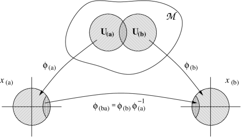
Figure 2: The manifold $\mathcal{M}$ is covered by patches $U_{(a)}$, parameterized by coordinates $x_{(a)}\in\mathbb{R}^{n}$. To go from one coordinate to another, one uses the transition functions $\phi_{(ba)}$.

Conversely, one can construct a manifold by giving a parametrization $x_{(a)}$ for a set of local charts $U_{(a)}$, and giving the transition functions $\phi_{(ba)}$ between the charts. However, these transition functions cannot be arbitrary functions. The reason is that in regions where three charts overlap, say $U_{(a)},U_{(b)}$ and $U_{(c)}$, one should be able to go from coordinates $x_{(a)}$ to coordinates $x_{(b)}$, then from $x_{(b)}$ to $x_{(c)}$, and finally from $x_{(c)}$ to $x_{(a)}$ again. Since in each step we are simply switching to different coordinates for the same point $P$ on the manifold, in the end we should be back at the same coordinates as the ones we started with. That is, one should have

$$\phi_{(ac)}\phi_{(cb)}\phi_{(ba)}=1$$ (2.2)

on triple overlaps $U_{(a)}\cap U_{(b)}\cap U_{(c)}$. This condition on the transition functions is called the cocycle condition, and it can be shown that this is the only condition one needs to put on the transition functions to obtain a well-defined manifold. (In particular, there are no extra conditions on overlaps of four or more patches, since all of these follow from (2.2).)

Of course, the above construction only guarantees that the transition functions we find are continuous and invertible. In practice, we would like to be able to differentiate functions on our manifold as often as we like, and hence one should require the transition functions to be $C^{\infty}$ (that is, infinitely many times differentiable) as well. The manifolds that allow such transition functions are called $C^{\infty}$-manifolds; we will always assume this property when we speak of a manifold.

All of this is straightforwardly generalized to complex manifolds: here, the coordinate functions $\phi_{(a)}$ should map $U_{(a)}$ to $\mathbb{C}^{m}$, and the transition functions must be holomorphic – that is, on an overlap $U_{(a)}\cap U_{(b)}$ the coordinates $z_{(b)}$ should be analytic functions of $z_{(a)}$, and hence be independent of $\overline{z}_{(a)}$. This condition ensures that holomorphic objects – that is, globally defined objects such as functions which only depend on $z$ but not on $\overline{z}$ – can be well-defined over the whole manifold.

2.3 Topological invariants

The main mathematical question that topology addresses is: when are two spaces topologically equivalent? That is: given a topological space $A$ and a topological space $B$, is there a continuous and invertible map $f:A\to B$? If such a map exists, it is called a homeomorphism, and the two spaces $A$ and $B$ are called homeomorphic. In the case that these maps are differentiable, as we will usually assume, we speak of diffeomorphisms.

In general, it is incredibly hard to decide whether or not two spaces are homeomorphic. This statement may come as a surprise, but anyone who has ever tried to put up the lights on a Christmas tree knows that topological issues can be highly nontrivial. Restricting to the topology of $d$-dimensional, compact (that is, closed and bounded) and connected manifolds, the only cases in which we have a complete understanding of topology are $d=0,1$ and $2$. The only compact and connected $0$-dimensional manifold is a point. A $1$-dimensional compact and connected manifold can either be a line element or a circle, and it is intuitively clear (and can quite easily be proven) that these two spaces are topologically different. In two dimensions, there is already an infinite number of different topologies: a two-dimensional, compact and connected surface can have an arbitrary number of handles and boundaries, and can either be orientable or non-orientable (see figure 3). Again, it is intuitively quite clear that two surfaces are not homeomorphic if they differ in one of these respects. On the other hand, it can be proven that any two surfaces for which these data are the same can be continuously mapped to one another, and hence this gives a complete classification of the possible topologies of such surfaces.

Figure 3: (a) The sphere is an orientable manifold without handles or boundaries. (b) An orientable manifold with one boundary and one handle. (c) The Möbius strip: an unorientable manifold with one boundary and no handles.

A quantity such as the number of boundaries of a surface is called a topological invariant. A topological invariant is a number, or more generally any type of structure, which one can associate to a topological space, and which does not change under continuous mappings. Topological invariants can be used to distinguish between topological spaces: if two surfaces have a different number of boundaries, they can certainly not be topologically equivalent. On the other hand, the knowledge of a topological invariant is in general not enough to decide whether two spaces are homeomorphic: a torus and a sphere have the same number of boundaries (zero), but are clearly not homeomorphic. Only when one has some complete set of topological invariants, such as the number of handles, boundaries and crosscaps (see footnote) in the two-dimensional case, is it possible to determine whether or not two topological spaces are homeomorphic.

In more than two dimensions, many topological invariants are known, but for no dimension larger than two has a complete set of topological invariants been found. In fact, in four or more dimensions such a set would consist of an uncountably infinite number of invariants! (I assume here that such an invariant is itself in a countable set, such as the set of all integers.) A general classification of topologies is therefore very hard to obtain, but even without such a general classification, each new invariant that can be constructed gives us a lot of interesting new information. For this reason, the construction of topological invariants is one of the most important issues in topology. The nature of these topological invariants can be quite diverse: in the case of two dimensions, we saw two topological invariants that were positive numbers (the numbers of handles and boundaries), and one that was an element of the set $\{0,1,2\}$: the number of necessary crosscaps. But topological invariants can also be polynomials, groups, or elements of a given group, for example.

As we will see in these notes, topological field and string theories can be used to construct certain topological invariants. Conversely, topologically invariant structures play an important role in the construction of topological field and string theories. The main examples of this last statement are homology and cohomology: two topological invariants which assign a group to a certain manifold. In the next section, we will briefly review these structures.

2.4 Homology and cohomology

2.4.1 Differential forms

Let us begin by recalling the notion of a $p$-form. A $p$-form is the mathematical equivalent of an antisymmetric tensor field living on a manifold $\mathcal{M}$. Consider a patch of $\mathcal{M}$ parameterized by $n$ real coordinates $x^{i}$. A $p$-form can now be written as

$$B(x)\equiv B_{i_{1}\ldots i_{p}}(x)\,dx^{i_{1}}\wedge dx^{i_{2}}\wedge\cdots\wedge dx^{i_{p}}.$$ (2.3)

Here, the $dx^{i}$ are so-called cotangent vectors at the point $x$. (For the definition of the $\wedge$-product, see below.) Formally, a cotangent vector is a linear map from the tangent vector space at $x$ to the real numbers. The cotangent vector $dx^{i}$ is the specific linear map that maps the unit tangent vector in the $x^{i}$-direction to 1, and all tangent vectors in the other coordinate directions to 0. From this, we see that a general linear map from the tangent vector space at $x$ to $\mathbb{R}$ can be written as

$$A(x)=A_{i}(x)\,dx^{i}.$$ (2.4)

In other words, the space of all one-forms is precisely the space of all cotangent vector fields! Note that at every point $x$, the possible values of a one-form make up an $n$-dimensional vector space with coordinates $A_{i}(x)$. As we will see in the next section, when we glue together all of these vector spaces for different $x$, we get what is called a vector bundle – in this particular case the “cotangent bundle”.

The $dx^{i}$-notation of course suggests a relation to integrals. This can be made precise as follows. Suppose we have a one-dimensional closed curve $\gamma$ inside $\mathcal{M}$. Let us show that a one-form $A(x)$ on $\mathcal{M}$ can then naturally be integrated along $\gamma$. Parameterize $\gamma$ by a parameter $t$, so that its coordinates are given by $x^{i}(t)$. At time $t$, the velocity $dx(t)/dt$ is a tangent vector to $\mathcal{M}$ at $x(t)$. One can insert this tangent vector into the linear map $A(x)$ to get a real number. By definition, inserting the vector $dx(t)/dt$ into the linear map $dx^{i}$ simply gives the component $dx^{i}(t)/dt$. Doing this for every $t$, we can then integrate over $t$:

$$\int\left(A_{i}(x(t))\frac{dx^{i}}{dt}\right)dt$$ (2.5)

It is clear that this expression is independent of the parametrization in terms of $t$. Moreover, from the way that tangent vectors transform, one can deduce how the linear maps $dx^{i}$ should transform, and from this how the coefficients $A_{i}(x)$ should transform. Doing this, one sees that the above expression is also invariant under changes of coordinates on $\mathcal{M}$. Therefore, a one-form can unambiguously be integrated over a curve in $\mathcal{M}$. We write such an integral as

$$\int_{\gamma}A_{i}(x)\,dx^{i}$$ (2.6)

or even shorter, as

$$\int_{\gamma}A$$ (2.7)

Of course, when $\mathcal{M}$ is itself one-dimensional, (2.5) gives precisely the ordinary integration of a function $A(x)$ over $x$, so the notation (2.6) is indeed natural.

Similarly, one would like to define a two-form as something which can naturally be integrated over a two-dimensional surface in $\mathcal{M}$. At a specific point $x$, the tangent plane to such a surface is spanned by a pair of tangent vectors, $(v^{1},v^{2})$. So to generalize the construction of a one-form, we should give a bilinear map from such a pair to $\mathbb{R}$. The most general form of such a map is

$$B_{ij}(x)\,dx^{i}\otimes dx^{j},$$ (2.8)

where the tensor product of two cotangent vectors acts on a pair of vectors as follows:

$$dx^{i}\otimes dx^{j}\,(v^{1},v^{2})=dx^{i}(v^{1})\,dx^{j}(v^{2}).$$ (2.9)

On the right hand side of this equation, one multiplies two ordinary numbers obtained by letting the linear map $dx^{i}$ act on $v^{1}$, and $dx^{j}$ on $v^{2}$.

The bilinear map (2.8) is slightly too general to give a good integration procedure, though. The reason is that we would like the integral to change sign if we change the orientation of integration, just like in the one-dimensional case. In two dimensions, changing the orientation simply means exchanging $v^{1}$ and $v^{2}$, so we want our bilinear map to be antisymmetric under this exchange. This is achieved by defining a two-form to be

$$B = B_{ij}(x)\,\left(dx^{i}\otimes dx^{j}-dx^{j}\otimes dx^{i}\right)$$ (2.10)

$$\equiv B_{ij}(x)\,dx^{i}\wedge dx^{j}$$

We now see why a two-form corresponds to an antisymmetric tensor field: the symmetric part of $B_{ij}$ would give a vanishing contribution to $B$. Now, parameterizing a surface $\Sigma$ in $\mathcal{M}$ with two coordinates $t_{1}$ and $t_{2}$, and reasoning exactly like we did in the case of a one-form, one can show that the integration of a two-form over such a surface is indeed well-defined, and independent of the parametrization of both $\Sigma$ and $\mathcal{M}$.

For $p$-forms of higher degree $p$, the construction goes in exactly the same way, where now the $\wedge$-product is a totally antisymmetric tensor product of $p$ cotangent vectors. In fact, one can use the wedge product to multiply an arbitrary $p$-form with an arbitrary $q$-form in the same way:

$$B^{(1)}\wedge B^{(2)}=B^{(1)}_{[i_{1}\ldots i_{p}}\,B^{(2)}_{i_{p+1}\ldots i_{p+q}]}\,dx^{i_{1}}\wedge\cdots\wedge dx^{i_{p+q}},$$ (2.11)

where the square brackets denote total antisymmetrization in the indices. (Of course, we do not strictly need this antisymmetrization in the formula, since the wedge product of the $dx^{i}$ is already antisymmetric.) Note that because of the antisymmetry, the maximal degree that a nonzero form can have is the dimension $n$ of $\mathcal{M}$.

2.4.2 De Rham cohomology

There is a natural notion of taking derivatives of $p$-forms. Since taking an $x^{i}$-derivative of an antisymmetric tensor adds an extra lower index, it is natural to construct a derivative that maps $p$-forms to $(p+1)$-forms. This derivative $d$ is called the exterior derivative, and it is defined as:

$$dB\equiv\frac{\partial B_{i_{1}\ldots i_{p}}}{\partial x^{j}}\,dx^{j}\wedge dx^{i_{1}}\wedge\cdots\wedge dx^{i_{p}}.$$ (2.12)

Because of the antisymmetry properties of the wedge product, we have that

$$d^{2}=0.$$ (2.13)

This simple formula leads to the important notion of cohomology. Let us try to solve the equation $dB=0$ for a $p$-form $B$. A trivial solution is $B=0$. From the above formula, we can actually easily find a much larger class of trivial solutions: $B=dA$ for a $(p-1)$-form $A$. More generally, if $B$ is any solution to $dB=0$, then so is $B+dA$. We want to consider these two solutions as equivalent:

$$B\sim B+B^{\prime}\qquad\mbox{if}\qquad B^{\prime}\in\mbox{Im}~{}d,$$ (2.14)

where $\mbox{Im}~{}d$ is the image of $d$, that is, the collection of all $p$-forms of the form $dA$. (To be precise, the image of $d$ of course contains $q$-forms for any $0<q\leq n$, so we should restrict this image to the $p$-forms for the $p$ we are interested in.) The set of all $p$-forms which satisfy $dB=0$ is called the kernel of $d$, denoted $\mbox{Ker~{}}d$, so we are interested in $\mbox{Ker~{}}d$ up to the equivalence classes defined by adding elements of $\mbox{Im}~{}d$. (Again, strictly speaking, $\mbox{Ker~{}}d$ consists of $q$-forms for several values of $q$, so we should restrict it to the $p$-forms for our particular choice of $p$.) This set of equivalence classes is called $H^{p}(\mathcal{M})$, the $p$-th cohomology group of $\mathcal{M}$:

$$H^{p}(\mathcal{M})=\frac{\mbox{Ker~{}}d}{\mbox{Im}~{}d}.$$ (2.15)

Clearly, $\mbox{Ker~{}}d$ is a group under addition: if two forms $B^{(1)}$ and $B^{(2)}$ satisfy $dB^{(1)}=dB^{(2)}=0$, then so does $B^{(1)}+B^{(2)}$. Moreover, if we change $B^{(i)}$ by adding some $dA^{(i)}$, the result of the addition will still be in the same cohomology class, since it differs from $B^{(1)}+B^{(2)}$ by $d(A^{(1)}+A^{(2)})$. Therefore, we can view this addition really as an addition of cohomology classes: $H^{p}(\mathcal{M})$ is itself an additive group. Also note that if $B^{(3)}$ and $B^{(4)}$ are in the same cohomology class (that is, their difference is of the form $dA^{(3)}$), then so are $cB^{(3)}$ and $cB^{(4)}$ for any constant factor $c$. In other words, we can multiply a cohomology class by a constant to obtain another cohomology class: cohomology classes actually form a vector space.

Now, we come to the reason why cohomology groups are so interesting for us. One important mathematical result is that for compact manifolds, the vector spaces $H^{p}(\mathcal{M})$ are in fact finite-dimensional. Their dimensions are called the Betti numbers $b^{p}$. Since there are no $p$-forms for $p>n$, we immediately see that $H^{p}(\mathcal{M})=0$ and hence $b^{p}=0$ for $p>n$, so this gives us a set of $n+1$ numbers which are possibly nonzero. Just like for integrals of $p$-forms, one can show that the exterior derivative of a $p$-form is independent of the coordinates we use, and hence of the notion of a distance on the manifold. As a result, the whole construction of the cohomology groups does not depend on such a notion: the cohomology groups are topological invariants! Since any two vector spaces of the same dimension are isomorphic, the only nontrivial information contained in $H^{p}(\mathcal{M})$ is really its dimension $b^{p}$, so one can just as well consider the set of Betti numbers $b^{p}$ to be a set of $n+1$ topological invariants.

Note that so far, the whole construction only depended on the following properties:

• $d^{2}=0$

• $d$ acts linearly on a graded vector space. That is, it maps objects of a certain degree $p$ to objects of degree $p+1$.

• The objects on which $d$ acts, and the way in which it acts, are independent of the choice of coordinates on $\mathcal{M}$. (Of course, the construction should also be independent of any other structure on $\mathcal{M}$, and in particular it should not involve a choice of metric.)

Therefore, for any other operator with these properties, we can create a similar structure and derive topological invariants from it. Many constructions of this type are known in mathematics and in physics, and they all go by the name of cohomology. The particular type of cohomology we introduced above is called “de Rham cohomology”. Of course, the requirement that $d$ maps objects of degree $p$ to objects of degree $p+1$ can just as well replaced by the requirement that it maps them to objects of degree $p-1$.

In general cohomology theories, objects of the form $dA$ are called “exact”, and objects for which $dB=0$ are called “closed”. We will use this terminology throughout these notes.

2.4.3 Homology

Another operator of the kind introduced above is the boundary operator $\delta$, which maps compact submanifolds of $\mathcal{M}$ to their boundary. Here, $\delta S=0$ means that a submanifold $S$ of $\mathcal{M}$ has no boundary, and $S=\delta U$ means that $S$ is itself the boundary of some submanifold $U$. It is intuitively clear, and not very hard to prove, that $\delta^{2}=0$: the boundary of a compact submanifold does not have a boundary itself. That the objects on which $\delta$ acts are independent of its coordinates is also clear. So is the grading of the objects: the degree $p$ is simply the dimension of the submanifold $S$. (Note that here we have an example of an operator that maps objects of degree $p$ to objects of degree $p-1$ instead of $p+1$.) What is less clear is that the collection of submanifolds actually forms a vector space, but one can of course always define this vector space to consist of formal linear combinations of submanifolds, and this is precisely how one proceeds. The $p$-dimensional elements of this vector space are called “$p$-chains”. One should think of $-S$ as $S$ with its orientation reversed, and of the sum of two disjoint sets, $S^{(1)}+S^{(2)}$, as their union. The equivalence classes constructed from $\delta$ are called homology classes. For example, in figure 4, $S^{(1)}$ and $S^{(2)}$ both satisfy $\delta S=0$, so they are elements of $\mbox{Ker~{}}\delta$. Moreover, it is clear that neither of them separately can be viewed as the boundary of another submanifold, so they are not in the trivial homology class $\mbox{Im}~{}\delta$. However, the boundary of $U$ is $S^{(1)}-S^{(2)}$. (The minus sign in front of $S^{(2)}$ is a result of the fact that $S^{(2)}$ itself actually has the wrong orientation to be considered a boundary of $U$.) This can be written as

$$S^{(1)}-S^{(2)}=\delta U,$$ (2.16)

or equivalently

$$S^{(1)}=S^{(2)}+\delta U,$$ (2.17)

showing that $S^{(1)}$ and $S^{(2)}$ are in the same homology class.

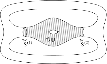
Figure 4: The 1-dimensional submanifolds $S^{(1)}$ and $S^{(2)}$ represent the same homology class, since their difference is the boundary of $U$.

The cohomology groups for the $\delta$-operator are called homology groups, and denoted by $H_{p}(\mathcal{M})$, with a lower index. (Of course historically, as can be seen from the terminology, homology came first and cohomology was related to it in the way we will discuss below. However, since the cohomology groups have a more natural additive structure, it is the name “cohomology” which is actually used for generalizations.) The $p$-chains $S$ that satisfy $\delta S=0$ are called $p$-cycles. Again, the $H_{p}(\mathcal{M})$ only exist for $0\leq p\leq n$.

There is an interesting relation between cohomology and homology groups. Note that we can construct a bilinear map from $H^{p}(\mathcal{M})\times H_{p}(\mathcal{M})\to\mathbb{R}$ by

$$\left([B],[S]\right)\mapsto\int_{S}B,$$ (2.18)

where $[B]$ denotes the cohomology class of a $p$-form $B$, and $[\Sigma]$ the homology class of a $p$-cycle $\Sigma$. Using Stokes’ theorem, it is easily seen that the result does not depend on the representatives for either $B$ or $S$:

$$\int_{S+\delta U}B+dA = \int_{S}B+\int_{S}dA+\int_{\delta U}B+dA$$ (2.19)

$$= \int_{S}B+\int_{\delta S}A+\int_{U}d(B+dA)$$

$$= \int_{S}B,$$

where we used that by the definition of (co)homology classes, $\delta S=0$ and $dB=0$. As a result, the above map is indeed well-defined on homology and cohomology classes. A very important theorem by de Rham says that this map is nondegenerate. This means that if we take some $[B]$ and we know the result of (2.18) for all $[S]$, this uniquely determines $[B]$, and similarly if we start by picking an $[S]$. This in particular means that the vector space $H^{p}(\mathcal{M})$ is the dual vector space of $H_{p}(\mathcal{M})$, and hence that the Betti number $b^{p}$ is also the dimension of $H_{p}(\mathcal{M})$.

2.4.4 The Hodge star and harmonic forms

Another important operator on $p$-forms is the Hodge star operator. It is defined as

$$*B={\epsilon^{i^{1}\ldots i^{p}}}_{j_{1}\ldots j_{n-p}}\,B_{i^{1}\ldots i^{p}}\,dx^{j_{1}}\wedge\cdots\wedge dx^{j_{n-p}}.$$ (2.20)

Note that the definition of this operator does use a metric on $\mathcal{M}$: it is used to lower indices of the $\epsilon$-tensor. It is therefore important to realize that constructions involving this operator do not automatically lead to topologically invariant results – though as we will see, in certain cases they do.

Since the Hodge star maps $p$-forms to $(n-p)$-forms, the wedge product of a $p$-form $B$ with the Hodge dual of another $p$-form $C$ can naturally be integrated over the whole manifold $\mathcal{M}$. In fact, it can be shown that

$$(B,C)\equiv\int_{\mathcal{M}}B\wedge*C$$ (2.21)

defines a nondegenerate and (on Euclidean manifolds) positive definite inner product on the space $\Omega^{p}(\mathcal{M})$ of $p$-forms for some fixed $p$. This can also be viewed as an inner product on the space $\Omega^{*}(\mathcal{M})$ of all forms if one defines the inner product of a $p$-form and a $q$-form for $p\neq q$ to vanish – that is, one takes the $\Omega^{p}(\mathcal{M})$ for different $p$ to be orthogonal to each other. We can then also define the adjoint operator of the exterior derivative with respect to this inner product. By definition, the adjoint operator $d^{*}$ is the operator which satisfies

$$(B,dC)=(d^{*}B,C).$$ (2.22)

That this uniquely defines the way in which the $d^{*}$-operator acts can be seen as follows. If we fix $B$ and require the above relation for all $C$, this relation tells us what $(d^{*}B,C)$ is for every $C$. Since the inner product is nondegenerate, this uniquely fixes $d^{*}B$ itself. By comparing the degrees in the above formulas, one sees that if $B$ is a $p$-form, $d^{*}B$ will be a $(p-1)$-form, so $d^{*}$ acts in the “opposite direction” compared to $d$.

It turns out that there is also a more direct expression for the adjoint operator acting on $p$-forms: it can be written as

$$d^{*}=(-1)^{pn+p+1}*d*,$$ (2.23)

Note that, also from this expression, it is clear that $d^{*}$ lowers the degree of a form by 1.

Now, let us make the simple observation that for a fixed $B$,

$$0 = (B,ddC)$$ (2.24)

$$= (d^{*}d^{*}B,C)$$

for any $C$. Using once again the fact that the inner product is nondegenerate, this means that $(d^{*})^{2}B=0$. Since $B$ was arbitrary, this means that

$$(d^{*})^{2}=0.$$ (2.25)

Does this mean that using the $d^{*}$-cohomology, we can define another set of topological invariants? At first sight, this is not clear, since we did not define $d^{*}$ in a metric-independent way. We will now argue that in fact the $d^{*}$-cohomology is a topological invariant, but that it gives exactly the same information as the $d$-cohomology.

Note that the operators $dd^{*}$ and $d^{*}d$ map $p$-forms to $p$-forms. One can show by writing out the definitions, including the omitted factors of $p!$, that

$$dd^{*}+d^{*}d=\Delta,$$ (2.26)

where $\Delta$ is the Laplacian acting on the components $B_{i_{1}\ldots i_{p}}$. We can now look for solutions to the equations $dB=d^{*}B=0$. An important theorem by Hodge states that each $d$-cohomology class contains exactly one such form $B_{h}$, which by the previous remark is a harmonic form: $\Delta B_{h}=0$. In other words, the $d$-cohomology classes are in one-to-one correspondence to the harmonic forms on $\mathcal{M}$. However, the Hodge theorem is symmetric, in the sense that it also predicts a unique harmonic form in each $d^{*}$-cohomology class. Therefore, both $H^{p}_{d}(\mathcal{M})$ and $H^{p}_{d^{*}}(\mathcal{M})$ can be identified with the vector space of harmonic $p$-forms, and hence we find the promised result that the two are equivalent.

2.4.5 Dolbeault cohomology

So far, we have been discussing real manifolds. However, there is an interesting generalization of all of this to complex manifolds, which is called “Dolbeault cohomology”. On complex $m$-dimensional manifolds, we have local coordinates $z^{i}$ and $\overline{z}^{i}$. One can now study $(p,q)$-forms, which are forms containing $p$ factors of $dz^{i}$ and $q$ factors of $d\overline{z}^{j}$:

$$B=B_{i_{1}\ldots i_{p},j_{1}\ldots j_{q}}(z,\overline{z})\,dz^{i_{1}}\wedge\cdots\wedge dz^{i_{p}}\wedge d\overline{z}^{j_{1}}\wedge\cdots\wedge d\overline{z}^{j_{q}}.$$ (2.27)

Moreover, one can introduce two exterior derivative operators $\partial$ and $\overline{\partial}$, where $\partial$ is defined by

$$\partial B\equiv\frac{\partial B_{i_{1}\ldots i_{p},j_{1}\ldots j_{q}}}{\partial z^{k}}\,dz^{k}\wedge dz^{i_{1}}\wedge\cdots\wedge dz^{i_{p}}\wedge d\overline{z}^{j_{1}}\wedge\cdots\wedge d\overline{z}^{j_{q}},$$ (2.28)

and $\overline{\partial}$ is defined similarly by differentiating with respect to $\overline{z}^{k}$ and adding a factor of $d\overline{z}^{k}$. Again, both of these operators square to zero. We can now construct two cohomologies – one for each of these operators – but as we will see, in the cases that we are interested in, the information contained in them is the same. Conventionally, one uses the cohomology defined by the $\overline{\partial}$-operator.

For complex manifolds, Hodge’s theorem also holds: each cohomology class $H^{p,q}(\mathcal{M})$ contains a unique harmonic form. Here, a harmonic form $B_{h}$ is a form for which the “Laplacian”

$$\Delta_{\overline{\partial}}=\overline{\partial}\overline{\partial}^{*}+\overline{\partial}^{*}\overline{\partial}$$ (2.29)

has a zero eigenvalue: $\Delta_{\overline{\partial}}B_{h}=0$. In general, this operator does not equal the ordinary Laplacian, but one can prove that in the case where $\mathcal{M}$ is a Kähler manifold,

$$\Delta=2\Delta_{\overline{\partial}}=2\Delta_{\partial}.$$ (2.30)

In other words, on a Kähler manifold the notion of a harmonic form is the same, independently of which exterior derivative one uses. As a first consequence, we find that the vector spaces $H^{p,q}_{\partial}(\mathcal{M})$ and $H^{p,q}_{\overline{\partial}}(\mathcal{M})$ both equal the vector space of harmonic $(p,q)$-forms, so the two cohomologies are indeed equal. Moreover, every $(p,q)$-form is of course a $(p+q)$-form in the de Rham cohomology, and by the above result we see that a harmonic $(p,q)$-form can also be viewed as a de Rham harmonic $(p+q)$-form. Conversely, any de Rham $p$-form can be written as a sum of Dolbeault forms:

$$B_{p}=B_{p,0}+B_{p-1,1}+\ldots+B_{0,p}.$$ (2.31)

Acting on this with the Laplacian, one sees that for a harmonic $p$-form,

$$0=\Delta B_{p}=\Delta_{\overline{\partial}}B_{p}=\Delta_{\overline{\partial}}B_{p,0}+\Delta_{\overline{\partial}}B_{p-1,1}+\ldots+\Delta_{\overline{\partial}}B_{0,p}.$$ (2.32)

Since $\Delta_{\overline{\partial}}$ does not change the degree of a form, $\Delta_{\overline{\partial}}B_{p_{1},p_{2}}$ is also a $(p_{1},p_{2})$-form. Therefore, the right hand side can only vanish if each term vanishes separately, so all the terms on the right hand side of (2.31) must be harmonic forms. Summarizing, we have shown that the vector space of harmonic de Rham $p$-forms is a direct sum of the vector spaces of harmonic Dolbeault $(p_{1},p_{2})$-forms with $p_{1}+p_{2}=p$. Since the harmonic forms represent the cohomology classes in a one-to-one way, we find the important result that for Kähler manifolds,

$$H^{p}(\mathcal{M})=H^{p,0}(\mathcal{M})\oplus H^{p-1,1}(\mathcal{M})\oplus\cdots\oplus H^{0,p}(\mathcal{M}).$$ (2.33)

That is, the Dolbeault cohomology can be viewed as a refinement of the de Rham cohomology. In particular, we have

$$b^{p}=h^{p,0}+h^{p-1,1}+\ldots+h^{0,p},$$ (2.34)

where $h^{p,q}=\dim H^{p,q}(\mathcal{M})$ are the so-called Hodge numbers of $\mathcal{M}$.

2.4.6 Relations between Hodge numbers and Poincaré duality

The Hodge numbers of a Kähler manifold give us several topological invariants, but not all of them are independent. In particular, the following two relations hold:

$$h^{p,q} = h^{q,p}$$

$$h^{p,q} = h^{m-p,m-q}.$$ (2.35)

The first relation immediately follows if we realize that $B\mapsto\overline{B}$ maps $\partial$-harmonic $(p,q)$-forms to $\overline{\partial}$-harmonic $(q,p)$-forms, and hence can be viewed as an invertible map between the two respective cohomologies. As we have seen, the $\partial$-cohomology and the $\overline{\partial}$-cohomology coincide on a Kähler manifold, so the first of the above two equations follows.

The second relation can be proven using the map

$$(A,B)\mapsto\int_{\mathcal{M}}A\wedge B$$ (2.36)

from $H^{p,q}\times H^{m-p,m-q}$ to $\mathbb{C}$. It can be shown that this map is nondegenerate, and hence that $H^{p,q}$ and $H^{m-p,m-q}$ can be viewed as dual vector spaces. (Compare the discussion at the end of section 2.4.3.) In particular, it follows that these vector spaces have the same dimension, which is the statement in the second line of (2.35).

Note that the last argument of course also holds for de Rham cohomology, in which case we find the relation $b^{p}=b^{n-p}$ between the Betti numbers. We also know that $H^{n-p}(\mathcal{M})$ is dual to $H_{n-p}(\mathcal{M})$, so combining these statements we find an identification between the vector spaces $H^{p}(\mathcal{M})$ and $H_{n-p}(\mathcal{M})$. This identification between $p$-form cohomology classes and $(n-p)$-cycle homology classes is known as Poincaré duality. Intuitively, it can be thought of as follows. Take a certain $(n-p)$-cycle $\Sigma$ representing a homology class in $H_{n-p}$. One can now try to define a “delta function” $\delta(\Sigma)$ which is localized on this cycle. Locally, $\Sigma$ can be parameterized by setting $p$ coordinates equal to zero, so $\delta(\Sigma)$ is a “$p$-dimensional delta function” – that is, it is an object which is naturally integrated over $p$-dimensional submanifolds: a $p$-form. This intuition can be made precise, and one can indeed view the cohomology class of the resulting “delta-function” $p$-form as the Poincaré dual to $\Sigma$.

Going back to the relations (2.35), we see that the Hodge numbers of a Kähler manifold can be nicely written in a so-called Hodge-diamond:

$$\begin{array}[]{ccccccc}&&&h^{0,0}\\ &&h^{1,0}&&h^{0,1}\\ &\mbox{\reflectbox{$\ddots$}}&&&&\ddots\\ h^{m,0}&&&\cdots&&&h^{0,m}\\ &\ddots&&&&\mbox{\reflectbox{$\ddots$}}\\ &&h^{m,m-1}&&h^{m-1,m}\\ &&&h^{m,m}\end{array}$$ (2.37)

The integers in this diamond are symmetric under the reflection in its horizontal and vertical axes.

2.5 Vector bundles

2.5.1 Definition

Vector bundles are the mathematical objects that describe vector fields in physics. A vector bundle $E$ over a manifold $\mathcal{M}$, denoted $E\to\mathcal{M}$, is a manifold which can be projected onto $\mathcal{M}$:

$$\pi:E\to\mathcal{M}$$ (2.38)

in such a way that the fiber $\pi^{-1}(x)$ at every point $x$ of $\mathcal{M}$ has the structure of a (fixed) vector space $W$. Locally – that is, on small enough patches $U_{(a)}$ for $\mathcal{M}$ – the vector bundle must look like $U_{(a)}\times W$, but this is not necessarily globally the case: the vector bundle does not need to be topologically equivalent to $\mathcal{M}\times W$. For example, a cylinder can be viewed as a vector bundle over the circle $S^{1}$, where the fiber $W$ is simply a line $\mathbb{R}$. This is a trivial vector bundle: the cylinder can be written as $S^{1}\times\mathbb{R}$. An example of a nontrivial vector bundle is the “infinite Möbius strip”, which can be obtained by taking the trivial vector bundle over an interval, e. g. $[0,1]\times\mathbb{R}$, and gluing $(0,y)$ to $(1,-y)$. This is again a vector bundle over the circle $S^{1}$, where this circle can be viewed as the set of points $(x,0)$, with $(0,0)$ and $(1,0)$ identified. The projection $\pi$ maps the fiber, consisting of the points $(x_{0},y)$ at fixed $x_{0}$, to the point $(x_{0},0)$ on the circle.

A section of a vector bundle is what a physicist would call a “field configuration”: it is a map from $\mathcal{M}$ to $E$ such that every point of $\mathcal{M}$ is mapped to a point in the fiber $W$ living at that point. See figure 5 for a graphical representation of these ideas.

Figure 5: A simple example of a vector bundle $E$: the cylinder. The circle $\mathcal{M}=S^{1}$ is the base space (the other two circles are only drawn to visualize the geometry), and the fibers $W$ are lines. $S$ is a section of this vector bundle.

Just as for manifolds, the easiest way to construct a vector bundle is to do it patch by patch. That is, one considers a set of charts $\{U_{(a)}\}$ covering $\mathcal{M}$, and constructs the so-called local trivializations

$$U_{(a)}\times W.$$ (2.39)

Now, one glues together the $U_{(a)}$ using the transition functions $\phi_{(ba)}$ of the manifold, but of course one also needs to glue the vectors $V_{(a)}(x_{(a)})$ in the fibers $W$ on the patch $U_{(a)}$ to the vectors $V_{(b)}(x_{(b)})$ of the fibers $W$ on the patch $U_{(b)}$. This is done by choosing an extra set of transition functions $\Lambda_{(ba)}$:

$$V_{(b)}(x_{(b)})=\Lambda_{(ba)}(x_{(a)})\,V_{(a)}(x_{(a)}).$$ (2.40)

Of course, on triple overlaps, these transition functions also have to satisfy the cocycle condition:

$$\Lambda_{(ac)}\Lambda_{(cb)}\Lambda_{(ba)}=1.$$ (2.41)

Again, this single condition on the transition functions turns out to be enough to make sure that one constructs a well-defined vector bundle.

If $W$ is an $k$-dimensional vector space, the transition functions $\Lambda_{(ba)}(x)$ are elements of $GL(k,\mathbb{R})$. However, one can of course study classes of vector bundles where the transition functions take values in a subgroup $G\subset GL(k,\mathbb{R})$. For example, if $W$ is equipped with an inner product (that is, if one has a natural notion of the length of a vector) then it is natural to consider only length-preserving transition functions, so one would take $G=O(k)$. In such a case, $G$ is called the structure group of the manifold.

2.5.2 Examples

In this section, we want to mention several examples of vector bundles which will be important to us in what follows.

The principal bundle

Our first example is in fact not a vector bundle, since its fiber is not a vector space, but a group. (A topological space of this more general kind is called a fiber bundle.).

Suppose we have a vector bundle $E$ over a manifold $\mathcal{M}$ with patches $U_{(a)}$ and fiber transition functions $\Lambda_{(ba)}$. Since $\Lambda_{(ba)}(x)$ is an element of the structure group $G$, we can construct a new fiber bundle with the group $G$ as a fiber, by taking local trivializations $U_{(a)}\times G$, and gluing them together with the same transition functions $\Lambda_{(ba)}$:

$$g_{(b)}(x_{(b)})=\Lambda_{(ba)}(x_{(a)})\,g_{(a)}(x_{(a)}).$$ (2.42)

The fiber bundle constructed in this way is called the principal bundle associated to $E$, and we will denote it by $\tilde{E}$. Note that if we know how the structure group acts on the fiber $W$, we can also go in the opposite direction and reconstruct $E$ from $\tilde{E}$. More generally, by choosing a different representation of $G$ – that is, a different vector space $W^{\prime}$ on which $G$ naturally acts – we can construct another vector bundle $E^{\prime}$ from $\tilde{E}$ by taking the action of the new transition functions $\Lambda^{\prime}_{(ba)}$ to be the action of $\Lambda_{(ba)}$ in the representation $W^{\prime}$. This is the reason for the name “principal bundle”: from it, we can construct a vector bundle for each representation of $G$. We will see examples of this below when we discuss tangent bundles and spin bundles.

The tangent bundle

The tangent bundle to a manifold is the vector bundle whose fiber at a point $x$ is the tangent space at $x$. Suppose we have two overlapping patches, $U_{(a)}$ and $U_{(b)}$. The coordinates are related by a transition function:

$$x^{i}_{(b)}=\phi^{i}_{(ba)}(x_{(a)}).$$ (2.43)

Using standard mathematical terminology, let us denote the unit tangent vector at $x$ in the $x^{i}_{(a)}$-direction by $\partial/\partial x^{i}_{(a)}$. A general tangent vector on the patch $U_{(a)}$ can now be expressed as

$$v=v^{i}_{(a)}(x)\,\frac{\partial}{\partial x^{i}_{(a)}}.$$ (2.44)

The reason for this notation is that one can identify the tangent vector $v$ with a directional derivative in the direction $v$, or from a more physical point of view, that tangent vectors transform in the same way as directional derivatives. However, from our point of view, the notation will be purely symbolic: we will not think of the $\partial/\partial x^{i}_{(a)}$ as actually acting as derivatives on anything.

The transformation rule for the components of a vector under a change of coordinates from $x_{(a)}$ to $x_{(b)}$ is well known:

$$v^{i}_{(b)}(x_{(b)})=\frac{\partial\phi^{i}_{(ba)}}{\partial x^{j}_{(a)}}\,v^{j}_{(a)}(x_{(a)}).$$ (2.45)

That is, the transition functions of the fibers are given by

$$\left(\Lambda_{(ba)}\right)^{i}_{~{}j}=\frac{\partial\phi^{i}_{(ba)}}{\partial x^{j}_{(a)}}=\frac{\partial x^{i}_{(b)}}{\partial x^{j}_{(a)}}.$$ (2.46)

At every point $x$, this defines an element $\Lambda_{(ba)}$ of $GL(n,\mathbb{R})$. Moreover, if we require the coordinate transition functions $\phi_{(ba)}$ to be length-preserving, $\Lambda_{(ba)}$ is actually an element of $O(n)$, and if our base manifold $\mathcal{M}$ is orientable and we require that $\phi_{(ba)}$ preserves orientation, $\Lambda_{(ba)}$ is an element of $SO(n)$. We will always be considering this last situation in what follows.

As we explained before, we can construct the principal bundle $\tilde{E}$ associated to the tangent bundle by replacing the fibers $\mathbb{R}^{n}$ by the structure group $G=SO(n)$, and gluing the fibers with the same transition functions (2.46). This bundle is also called the frame bundle. Now, let us assume we have a different representation $W^{\prime}$ of $SO(n)$. For example, instead of vectors $v^{i}$, the elements of $W^{\prime}$ may be tensors with two indices, $T^{ij}$, so $W^{\prime}$ has dimension $n^{2}$. From the way that tensors transform under coordinate transformations, we see that the new transition functions of the bundle $E^{\prime}$ will be

$$\left(\Lambda^{\prime}_{(ba)}\right)^{ij}_{~{}~{}kl}=\left(\Lambda_{(ba)}\right)^{i}_{~{}k}\left(\Lambda_{(ba)}\right)^{j}_{~{}l}.$$ (2.47)

Similarly, from the frame bundle $\tilde{E}$ we can define vector bundles for tensor fields with an arbitrary number of upper and lower indices. In particular, since $p$-forms have $p$ lower indices and are antisymmetric in these indices, we can view a $p$-form as a section of a vector bundle with $\binom{n}{p}$-dimensional fibers.

Since an $m$-dimensional complex manifold can be viewed as a $2m$-dimensional real manifold, it has a $2m$-dimensional tangent bundle. The most natural way to write the elements of this tangent bundle in terms of coordinates is of course

$$v=v^{i}_{(a)}(z,\overline{z})\,\frac{\partial}{\partial z^{i}_{(a)}}+v^{\overline{\imath}}_{(a)}(z,\overline{z})\,\frac{\partial}{\partial\overline{z}^{i}_{(a)}}.$$ (2.48)

Here, $v^{i}_{(a)}$ and $v^{\overline{\imath}}_{(a)}$ are complex conjugates. However, since we are working with complex coordinates, it is now natural to also study the complexified tangent bundle, where we allow the coordinates $v^{i}_{(a)}$ and $v^{\overline{\imath}}_{(a)}$ to be arbitrary, unrelated complex numbers. Note that this construction effectively doubles the dimension: a complex manifold with $m$ complex dimensions has a complexified tangent bundle with $2m$ complex-dimensional fibers. Also, note that in this construction we have not changed the transition functions: these still take values in $SO(2m,\mathbb{R})$. The only difference is that the elements of $SO(2m,\mathbb{R})$ now act on complex 2$m$-dimensional vectors.

A particular phenomenon appears in the case of a complex manifold of complex dimension 1. The structure group is then $SO(2)=U(1)$. The irreducible representations of $U(1)$ are one-dimensional, and therefore the vector representation in this case is not irreducible. This can easily be seen by writing an arbitrary vector as in (2.48), where the index $i$ now only takes a single value: clearly, the first term in (2.48) has charge 1 under $U(1)$, and the second term has charge $-1$. (Of course, this statement is true in any dimension, but it is only in two dimensions that the $U(1)$ is the full structure group of the tangent bundle.) Since the split-up into holomorphic and anti-holomorphic coordinates is globally defined, the whole two-dimensional complexified tangent bundle can be split up into the sum of two one-dimensional subbundles with complex conjugate transition functions. We denote these two bundles by $T^{+}\mathcal{M}$ and $T^{-}\mathcal{M}$.

Spin bundles

Since we now know how to construct vector bundles corresponding to arbitrary representations of $SO(n)$, a natural question is: what about spinor representations? Strictly speaking of course, spinors do not transform in a representation of $SO(n)$, but in a representation of $Spin(n)$, which is a double cover of the group $SO(n)$. The best known example of this is the case of $Spin(3)=SU(2)$ which is a double cover of $SO(3)$. Therefore, we would like to construct a principal bundle with fibers $Spin(3)$ from the tangent bundle. However, the transition functions $\Lambda_{(ba)}(x)$ are elements of $SO(n)$, and not of $Spin(n)$. More precisely, there are two elements in $Spin(n)$ corresponding to each single element in $SO(n)$, and these two elements differ by a sign. Therefore, to “lift” the transition functions $\Lambda_{(ba)}$ of the tangent (or frame) bundle $T\mathcal{M}$ to transition functions $\tilde{\Lambda}_{(ba)}$ for a spin bundle, we need to make a choice of sign for each pair $(ba)$. This leads to a large arbitrariness in the construction, but of course many of these arbitrary choices may lead to topologically equivalent bundles. What is more important, however, is that some choices of signs are simply not allowed. The reason is that to result in a well-defined vector bundle, the transition functions $\tilde{\Lambda}_{(ba)}$ have to satisfy the cocycle condition:

$$\tilde{\Lambda}_{(ac)}\tilde{\Lambda}_{(cb)}\tilde{\Lambda}_{(ba)}=1.$$ (2.49)

By choosing arbitrary signs, we might get $-1$ on the left hand side of this equation for some triple overlaps of patches, so this gives a certain number of conditions on the signs we choose. It may even happen that no choice of signs is consistent with the requirement (2.49), so it will be impossible to define a spin bundle! An example of a manifold where this happens is the two-dimensional complex projective space $\mathbb{C}P^{2}$. The manifolds on which it is possible to define a spin bundle are called “spin manifolds”. In general, such a manifold can allow several inequivalent choices of signs for $\tilde{\Lambda}_{(ba)}$, and these different choices are called spin structures. As an example, on a compact, orientable Riemann surface, for each homology one-cycle we have a free choice of sign, and so there are $2^{b^{1}}$ spin structures, and hence the same number of different spin bundles over the manifold.

It is possible to construct topological invariants on a manifold $\mathcal{M}$ which determine if a spin structure exists (the so-called Stiefel-Whitney classes), but we will not go into this. From now on, we will simply assume that a spin structure exists on our manifolds. In particular, as we mentioned, for two-dimensional orientable manifolds this is no restriction at all.

Another important property of the two-dimensional case is that, since the tangent bundle splits into two bundles $T^{+}\mathcal{M}$ and $T^{-}\mathcal{M}$, one can also split the spin bundle (for a given choice of spin structure) into two bundles with complex conjugate transition functions. These bundles are denoted $S^{+}(\mathcal{M})$ and $S^{-}(\mathcal{M})$. As it is usually assumed that a spin structure on $\mathcal{M}$ is chosen once and for all, the dependence on a choice of spin structure is not reflected in this notation.

Lie algebra valued one-forms

Finally, we want to construct a bundle which will be very important when we study connections in the next section. It is a bundle of Lie algebra-valued one-forms. Recall that an element of the Lie algebra $\mathfrak{g}$ of a group $G$ is a tangent vector to the group near the identity element. That is, if we have a curve $g(t)$ inside the group manifold such that $g(0)=e$, where $e$ is the identity element of the group, then the “velocity” at $t=0$,

$$\left.\frac{dg}{dt}\right|_{t=0},$$ (2.50)

is an element of the Lie algebra. More generally, at arbitrary “time” $t$ one can construct a Lie algebra element by “translating back to the origin”: both

$$g^{-1}\frac{dg}{dt}\qquad\mbox{and}\qquad\frac{dg}{dt}g^{-1}$$ (2.51)

are elements of the Lie algebra for any time $t$. Note that there are two inequivalent ways of translating back to the origin; it turns out that, for our purposes, the second one is the right one. For notational reasons, we “partially integrate” this expression by subtracting $0=d(gg^{-1})/dt$, and write it as

$$-g\frac{dg^{-1}}{dt}.$$ (2.52)

We could of course have removed the minus sign by a different choice of convention, but this will also turn out to be notationally convenient in what follows.

Now assume we have a vector bundle $E$ with structure group $G$ and principal bundle $\tilde{E}$. Consider a section $g(x)$ of the principal bundle – that is, a group-valued “function” on the base manifold $\mathcal{M}$. On a certain patch $U_{(a)}$, we can now construct a Lie algebra valued one-form by considering

$$-g_{(a)}\,dg^{-1}_{(a)}=-g_{(a)}\frac{dg^{-1}_{(a)}}{dx^{i}}\,dx^{i}.$$ (2.53)

This is a one-form on $\mathcal{M}$, and by comparing with (2.52), it is clear that its coefficients are elements of the Lie algebra $\mathfrak{g}$. Of course, there are many Lie algebra valued one-forms that cannot be constructed in this way, but the reason we constructed these particular ones is that we can read off from them what the transition functions for objects of this type are. To see this, suppose we now have a neighboring patch $U_{(b)}$. We know from (2.42) how $g_{(b)}$ is constructed out of $g_{(a)}$. Inserting this in the above expression, we find that

$$-g_{(b)}\,dg^{-1}_{(b)} = -\Lambda_{(ba)}g_{(a)}\,d\left(g^{-1}_{(a)}\Lambda^{-1}_{(ba)}\right)$$ (2.54)

$$= -\Lambda_{(ba)}g_{(a)}\,dg^{-1}_{(a)}\Lambda^{-1}_{(ba)}-\Lambda_{(ba)}d\Lambda^{-1}_{(ba)}.$$

That is, the particular Lie algebra valued one-forms we have constructed naturally live in a fiber bundle with transition functions

$$A_{(b)}=\Lambda_{(ba)}A_{(a)}\Lambda^{-1}_{(ba)}-\Lambda_{(ba)}d\Lambda^{-1}_{(ba)}.$$ (2.55)

Note that strictly speaking, this is not a vector bundle: even though $A(x)$ can be viewed as an element of a vector space, the transition functions are not linear in $A(x)$. Also note that many other bundles of Lie algebra valued $p$-forms can be constructed. In particular, one might take transition functions of the form

$$B_{(b)}=\Lambda_{(ba)}B_{(a)}\Lambda^{-1}_{(ba)}$$ (2.56)

to construct a bundle of $p$-forms for arbitrary $p$. Since these transition functions are linear in $B$, contrary to the example above, this bundle is a vector bundle.

2.5.3 Connections

An important extra structure one can put on a vector bundle is that of a connection. A connection tells us how to parallel transport a vector at a point $x\in\mathcal{M}$ to a vector at a point $x^{\prime}\in\mathcal{M}$ along a curve $\gamma$. Note that, a priori, there is no well-defined way to compare the fibers at two different points of $\mathcal{M}$, so one indeed needs some extra structure to make this parallel transport well-defined.

Of course, to parallel transport vectors along curves, it is enough if we can define parallel transport under an infinitesimal displacement: given a vector $V$ at $x$, we would like to define its parallel transported version $\hat{V}$ after an infinitesimal displacement by $\epsilon v$, where $v$ is a tangent vector to $\mathcal{M}$. By the definition of the cotangent vector $dx^{i}$, the new coordinates will then be $\hat{x}^{i}=x^{i}+\epsilon dx^{i}(v)$. We could of course write $dx^{i}(v)$ as $v^{i}$, but it will be useful to keep the one-form notation explicit. The infinitesimal change in the vector will be linear in the displacement and in $V$, so it will be of the form

$$\hat{V}^{I}(\hat{x})=V^{I}(x)+\epsilon A^{I}_{Ji}(x)V^{J}(x)dx^{i}(v).$$ (2.57)

If we take $A^{I}_{Ji}(x)dx^{i}$ to be a one-form, this expression is independent of our choice of coordinates for $\mathcal{M}$. However, we would like it to be independent of the choice of coordinates on the fiber $W$ as well. To achieve this, let us act on the above equation with a position-dependent group element $g^{I}_{J}(x)$. To linear order in $\epsilon$, the left hand side then becomes

LHS $$\to g^{I}_{J}(\hat{x})\,\hat{V}^{J}(\hat{x})$$ (2.58)

$$= g^{I}_{J}(x)\hat{V}^{J}(\hat{x})+\epsilon\frac{dg^{I}_{J}}{dx^{i}}(x)\,dx^{i}(v)\hat{V}^{J}(\hat{x})$$

$$= g^{I}_{J}(x)\hat{V}^{J}(\hat{x})+\epsilon\,dg^{I}_{J}(v)\,V^{J}(x)$$

where in the last line we inserted (2.57) and the definition of $dg$. Acting on the right hand side of (2.57) with $g^{I}_{J}(x)$ gives

RHS $$\to g^{I}_{J}(x)V^{J}(x)+\epsilon\tilde{A}^{I}_{Ji}(x)g^{J}_{~{}K}(x)V^{K}(x)\,dx^{i}(v),$$ (2.59)

where we denoted the transformed version of $A$ by $\tilde{A}$. Equating the last two results, and multiplying by $g^{-1}(x)$, we find that

$$\hat{V}(\hat{x})=V(x)+\epsilon\left(g^{-1}\tilde{A}(v)\,g-g^{-1}dg(v)\right)V(x),$$ (2.60)

where we left out the $I$-indices and wrote $\tilde{A}$ as a one-form to keep the formula readable. When comparing this to (2.57), we see that $A$ should transform as

$$\tilde{A}=gAg^{-1}-gdg^{-1}.$$ (2.61)

Note that this is precisely the transformation (2.55)! That is, for the parallel transport to be independent of the coordinates on $W$, we need $A$ to be a section of the bundle of Lie algebra valued one-forms defined by that equation. Of course, all of this was carried out with $V$ in a specific representation of $G$, but by starting from the defining representation of the structure group $G$, we can use the same connection to define parallel transport on vector bundles for any representation.

From its index structure and the way it transforms, $A^{I}_{Ji}$ looks very similar to a non-abelian gauge field. Let us show that this is exactly what it is. Suppose we have a vector field $V(x)$ on $\mathcal{M}$, and we want to define its derivative in the direction $v$ in a coordinate independent way. We would like to write down

$$\partial_{v}V(x)=\lim_{\epsilon\to 0}\frac{V(\hat{x})-V(x)}{\epsilon},$$ (2.62)

but here we are subtracting two vectors at different points in the numerator – an operation which is clearly dependent on our choice of coordinates. Therefore, the right thing to do is to first parallel transport $V(x)$ to $\hat{V}(\hat{x})$ and then subtract the two vectors. That is,

$$D_{v}V(x) = \lim_{\epsilon\to 0}\frac{V(\hat{x})-\hat{V}(\hat{x})}{\epsilon}$$ (2.63)

$$= \lim_{\epsilon\to 0}\frac{V(\hat{x})-V(x)-\epsilon A_{i}V(x)dx^{i}(v)}{\epsilon}$$

$$= \left(\partial_{i}V(x)-A_{i}V(x)\right)\,v^{i},$$

which is precisely the definition of a covariant derivative in terms of a gauge field $A$.

2.5.4 Chern classes

Inspired by the identification of a connection with a gauge field, let us consider the analogue of the non-abelian field strength:

$$F=dA-A\wedge A,$$ (2.64)

where $A\wedge A$ is a shorthand for $A^{I}_{Ji}A^{J}_{Kj}\,dx^{i}\wedge dx^{j}$. (Note that $A\wedge A\neq 0$, contrary to what the notation might suggest!) A short calculation shows that on the overlap of two patches of $\mathcal{M}$ (or equivalently, under a gauge transformation), this quantity transforms as

$$F_{(b)}=\Lambda_{(ba)}F_{(a)}\Lambda_{(ba)}^{-1}.$$ (2.65)

This is exactly the transformation (2.56), and we see that $F$ can be viewed as a section of a true vector bundle of Lie algebra valued two-forms! In particular, we can take its trace and obtain a genuine two-form:

$$c_{1}=\frac{i}{2\pi}\mbox{Tr}(F),$$ (2.66)

where the prefactor is convention. It is easily seen that this two-form is closed:

$$d(\mbox{Tr}(F))=\mbox{Tr}(dF)=-\mbox{Tr}(d(A\wedge A))=-\mbox{Tr}(dA\wedge A-A\wedge dA)=0.$$ (2.67)

Therefore, we can take its cohomology class, for which we would like to argue that it is a topological invariant. It is clear that this construction is independent of the choice of coordinates on $\mathcal{M}$. Moreover, it is independent of gauge transformations of the form (2.61). However, on a general vector bundle there may of course be connections which cannot be reached in this way from a given connection. Changing to such a connection is called a “large gauge transformation”, and from what we have said it is not clear a priori that the Chern classes do not depend on this choice of “equivalence class” of connections. However, with some work we can also prove this fact. The invariant $[c_{1}]$ is called the first Chern class. In fact, it might be better to call it a “relative topological invariant”: given a base manifold $\mathcal{M}$ of fixed topology, we can topologically distinguish vector bundles over it by calculating the above cohomology class.

Of course, by taking the trace of $F$, we loose a lot of information. There turns out to be a lot more topological information in $F$, and it can be extracted by considering the expression

$$c(F)=\det\left(1+\frac{iF}{2\pi}\right),$$ (2.68)

where $1$ is the identity matrix of the same size as the elements of the Lie algebra of $G$. Again, it can be checked that this expression is invariant under a change of coordinates for $\mathcal{M}$ and under a change of connection. Since the matrix components inside the determinant consist of the zero-form 1 and the two-form $F$, expanding the determinant will lead to an expression consisting of forms of all even degrees. One writes this as

$$c(F)=c_{0}(F)+c_{1}(F)+c_{2}(F)+\ldots$$ (2.69)

The sum terminates either at the highest degree encountered in expanding the determinant, or at the highest allowed even form on $\mathcal{M}$. Note that $c_{0}(F)=1$, and $[c_{1}(F)]$ is exactly the first Chern class we defined above. The cohomology class of $c_{n}$ is called the $n$th Chern class.

As an almost trivial example, let us consider the case of a product bundle $\mathcal{M}\times W$. As we have mentioned in the previous section, in this case there is a global section $g(x)$ of the principal bundle $\tilde{E}$, and we can use this to construct a connection $A=-gdg^{-1}$. Now we find that

$$F = -dgdg^{-1}-gdg^{-1}gdg^{-1}$$ (2.70)

$$= -dgdg^{-1}+dgdg^{-1}$$

$$= 0,$$

where in the second line we did a “partial integration” in the second term. Therefore, for a trivial bundle with this connection, $c_{0}=1$ and $c_{n}=0$ for all $n>0$.

3 Topological field theories – generalities

3.1 General definition

There exists a mathematically rigorous, axiomatic definition of topological field theories due to M. Atiyah. Instead of giving this definition, we will define topological field theory in a more physical, but as a result somewhat less rigorous way. The reader interested in the mathematical details is referred to [3].

The output of a quantum field theory is given by its observables: correlation functions of products of operators,

$$\langle\mathcal{O}_{1}(x_{1})\cdots\mathcal{O}_{n}(x_{n})\rangle_{b}.$$ (3.1)

Here, the $\mathcal{O}_{i}(x)$ are physical operators of the theory. What one calls “physical” is of course part of the definition of the theory, but it is important to realize that in general not all combinations of fields are viewed as physical operators. For example, in a gauge theory, we usually require the observables to arise from gauge-invariant operators. That is, $\mbox{Tr}~{}F$ would be one of the $\mathcal{O}_{i}$, but $\mbox{Tr}~{}A$ or $A$ itself would not.

The subscript $b$ in the above formula serves as a reminder that the correlation function is usually calculated in a certain background. That is, the definition of the theory may involve a choice of a manifold $\mathcal{M}$ on which the theory lives, it may involve choosing a metric on $\mathcal{M}$, it may involve choosing certain coupling constants, and so on.

The definition of a topological field theory is now as follows. Suppose that we have a quantum field theory where the background choices involve a choice of manifold $\mathcal{M}$ and a choice of metric $h$ on $\mathcal{M}$. Then the theory is called a topological field theory if the observables (3.1) do not depend on the choice of metric $h$. Let us stress that it is part of the definition that $h$ is a background field – in particular, we do not integrate over $h$ in the path integral. One may of course wonder what happens if, once we have a topological field theory, we do make the metric $h$ dynamical and integrate over it. This is exactly what we will do once we start considering topological string theories.

Note that the word “topological” in the definition may be somewhat of a misnomer. The reason is that the above definition does not strictly imply that the observables depend only on the topology of $\mathcal{M}$ – there may be other background choices hidden in $b$ on which they depend as well. For example, in the case of a complex manifold $\mathcal{M}$, correlation functions will in general not only depend on the topology of $\mathcal{M}$ and its metric, but also on our specific way of combining the $2d$ real coordinates on $\mathcal{M}$ into $d$ complex ones. This choice, called a complex structure, is part of the background of the quantum field theory, and correlation functions in a topological field theory will in general still depend on it.

If our quantum field theory has general coordinate invariance, as we will usually assume to be the case, then the above definition has an interesting consequence. The reason is that in such a case we can do an arbitrary general coordinate transformation, changing both the coordinates on $\mathcal{M}$ and its metric, under which the correlation functions should be invariant. Then, using the topological invariance, we can transform back the metric to its old value. The combined effect is that we have only changed the $x_{i}$ in (3.1). That is, in a generally coordinate invariant topological field theory, the observables do not depend on the insertion points of the operators.

3.2 Chern-Simons theory

The easiest way to construct a topological field theory is to construct a theory where both the action (or rather the “quantum measure” $e^{iS}$) and the fields do not include the metric at all. Such topological field theories are called “Schwarz-type” topological field theories. This may sound like a trivial solution to the problem, but nevertheless it can lead to quite interesting results! To see this, let us consider an example: Chern-Simons theory on a three-dimensional manifold $\mathcal{M}$.

Chern-Simons theory is a gauge theory – that is, in the language developed in the previous chapter, it is constructed from a vector bundle $E$ over the base space $\mathcal{M}$, with a structure group (gauge group) $G$ and a connection (gauge field) $A$. The Lagrangean of Chern-Simons theory is then given by

$$L=\mbox{Tr}\left(A\wedge dA-\frac{2}{3}A\wedge A\wedge A\right).$$ (3.2)

It is a straightforward exercise to check how this Lagrangean changes under the gauge transformation (2.61), and one finds

$$\tilde{L} \equiv \mbox{Tr}\left(\tilde{A}\wedge d\tilde{A}-\frac{2}{3}\tilde{A}\wedge\tilde{A}\wedge\tilde{A}\right)$$

$$= \mbox{Tr}\left(A\wedge dA-\frac{2}{3}A\wedge A\wedge A\right)-d\,\mbox{Tr}(gA\wedge dg^{-1})+\frac{1}{3}\mbox{Tr}(gdg^{-1}\wedge dg\wedge dg^{-1}).$$

The second term is a total derivative, so if $\mathcal{M}$ does not have a boundary, the action, being the integral of $L$ over $\mathcal{M}$, does not get a contribution from this term. The last term is not a total derivative, but its integral turns out to be a topological invariant of the map $g(x)$, which is quantized as

$$\frac{1}{24\pi^{2}}\int_{\mathcal{M}}\mbox{Tr}(gdg^{-1}\wedge dg\wedge dg^{-1})=m\in\mathbb{Z}.$$ (3.4)

From this, we see that if we define the action as

$$S=\frac{k}{4\pi}\int_{\mathcal{M}}L,$$ (3.5)

with $k$ an integer, the action changes by $2\pi km$ under gauge transformations, and the quantum measure $e^{iS}$ is invariant.

So from this discussion we seem to arrive at the conclusion that the partition function

$$Z=\int DA\,e^{iS[A]}$$ (3.6)

for a line bundle of a fixed topology $E$ is a topological invariant of $\mathcal{M}$, as are the correlation functions of gauge-invariant operators such as $\mbox{Tr}~{}F$. However, there is one more detail we have to worry about: there may be an anomaly in the quantum theory. That is, it may not be possible to define the path integral measure $DA$ in a gauge-invariant way.

One way to see what problems can arise is to note that to actually calculate the path integral, one has to pick a gauge condition on $A$. That is, we have to pick one representative of $A$ in each equivalence class under gauge transformations. To make such a choice will in general require a choice of metric. For example, from electromagnetism (where $E$ is a one-dimensional complex line bundle and $G=U(1)$) we know that a useful gauge is the Feynman gauge, in which the equation of motion for $A$ becomes

$$\Delta A=0.$$ (3.7)

As we have seen before, the Laplacian $\Delta$ is an operator which, through the Hodge star, depends on the metric, and hence the results we find will a priori be metric dependent. To show that the results are truly metric independent, one needs to show that the quantum results do not depend on our arbitrary choice of gauge.

We will not go into the details of this, but simply state that one can show that Chern-Simons theory on a compact three-manifold is anomaly-free, so our naive argument above was correct, and one can indeed calculate topological invariants of $\mathcal{M}$ in this way.

Let us briefly discuss the kind of topological invariants that Chern-Simons theory can lead to. Recall that one can construct a Lie group element $g$ from a Lie algebra element $\mathcal{A}$ as follows:

$$g=e^{\mathcal{A}}.$$ (3.8)

Now suppose we have a path $\gamma(t)$ inside $\mathcal{M}$. Suppose that we chop up $\gamma$ into very small line elements given by tangent vectors

$$\frac{d\gamma}{dt}\delta t$$ (3.9)

Then we can insert this tangent vector into the connection one-form $A$, and obtain a Lie algebra element. As we have seen, it is precisely this Lie algebra element which transports vectors in $E$ along this small distance: we have to multiply these vectors by $1+\mathcal{A}$. Of course, this is a linear approximation to the finite transformation $e^{\mathcal{A}}$. So if we transport a vector along the entire closed curve $\gamma$, it will return multiplied by a group element

$$g=\lim_{\delta t\to 0}\left[\exp\left(A\left(\frac{d\gamma}{dt}(0)\right)\delta t\right)\exp\left(A\left(\frac{d\gamma}{dt}(\delta t)\right)\delta t\right)\exp\left(A\left(\frac{d\gamma}{dt}(2\delta t)\right)\delta t\right)\cdots\right].$$ (3.10)

Now it is tempting to add all the exponents and write their sum in the limit as an integral, but this is not quite allowed since the different group elements may not commute, so $e^{X}e^{Y}\neq e^{X+Y}$. Therefore, one uses the following notation for this type of expression:

$$g=P\exp\int_{\gamma}A$$ (3.11)

where $P$ stands for path ordering. The element $g$ is called the holonomy of $A$ around the closed curve $\gamma$. An interesting gauge and metric independent object turns out to be the trace of this group element. This trace is called the Wilson loop $W_{\gamma}(A)$:

$$W_{\gamma}(A)=\mbox{Tr}~{}P\exp\int_{\gamma}A.$$ (3.12)

The topological invariants we are interested in are now the correlation functions of such Wilson loops in Chern-Simons theory. Since these correlation functions are independent of the parametrization of $\mathcal{M}$, we can equivalently say that they will be independent of the precise location of the loop $\gamma$; we have in fact constructed a topological invariant of the embedding of $\gamma$ inside $\mathcal{M}$! This embedding takes the shape of a knot, so the invariants we have constructed are knot invariants. One can show that the invariants are actually polynomials in the variable $y=\exp{2\pi i/(k+2)}$, where $k$ is the integer “coupling constant” of the Chern-Simons theory.

The above construction is due to E. Witten, and was carried out in [40] in 1988. Before Witten’s work, several polynomial invariants of knots were known, one of the simplest ones being the so-called Jones polynomial. It can be shown that many of these polynomials arise as special cases of the above construction, where one takes a certain structure group $G$, $SU(2)$ for the Jones polynomial, and a certain vector bundle (representation) $E$, the fundamental representation for the Jones polynomial. That is, using this “trivial” topological field theory, Witten was able to reproduce a large number of the known knot invariants in a unified framework, and construct a huge number of new invariants as well!

3.3 Cohomological field theories

Of course, even though the above example leads to quite interesting topological invariants, the construction itself is somewhat trivial: given the absence of anomalies that we mentioned, the independence of the metric is completely manifest throughout the procedure. There exists a different way of constructing topological field theories in which the definition of the theory does use a metric, but one can still show that the partition function and the physical correlation functions of the theory are metric-independent. The theories constructed in this way are called topological theories of “Witten-type”, or cohomological field theories.

Cohomological field theories are field theories that possess a very special type of symmetry. Recall that from Noether’s theorem a global symmetry of a theory leads to a conserved charge $S$, and that after quantizing the theory, the symmetry is generated by the corresponding operator:

$$\delta_{\epsilon}\mathcal{O}_{i}=i\epsilon[S,\mathcal{O}_{i}]\qquad\mbox{or}\qquad\delta_{\epsilon}\mathcal{O}_{i}=i\epsilon\{S,\mathcal{O}_{i}\},$$ (3.13)

depending on whether $S$ and $\mathcal{O}_{i}$ are fermionic or bosonic. Furthermore, the symmetry-invariant states $|j\rangle$ satisfy

$$S\,|j\rangle=0.$$ (3.14)

In particular, if the symmetry is not spontaneously broken, the vacuum of such a theory will be symmetric:

$$S\,|0\rangle=0,$$ (3.15)

and expectation values of operators will be unchanged after a symmetry transformation:

$$\langle 0|\mathcal{O}_{i}+\delta\mathcal{O}_{i}|0\rangle = \langle 0|\mathcal{O}_{i}|0\rangle+i\epsilon\langle 0|S\mathcal{O}_{i}\pm\mathcal{O}_{i}S|0\rangle$$ (3.16)

$$= \langle 0|\mathcal{O}_{i}|0\rangle,$$

since $S$ annihilates the vacuum. Note that, to linear order in $\epsilon$, the second term in the first line (with $|0\rangle$ replaced by an arbitrary state $|\psi\rangle$) can also be obtained if instead of on the operators, we let the symmetry operator $S$ act on the state as

$$|\psi\rangle\to|\psi\rangle+i\epsilon S|\psi\rangle.$$ (3.17)

In case $S$ is the Hamiltonian, this is the infinitesimal version of the well-known transition between the Schrödinger and Heisenberg pictures. Note that the equations (3.14) and (3.17) already contain some flavor of cohomology. Cohomological field theories are theories where this analogy can be made exact.

With this in mind, the first property of a cohomological field theory will not come as a surprise: it should contain a fermionic symmetry operator $Q$ which squares to zero,

$$Q^{2}=0.$$ (3.18)

This may seem like a strange requirement for a field theory, but symmetries of this type occur for example when we have a gauge symmetry and fix it by using the Faddeev-Popov procedure; the resulting theory will then have a global symmetry called BRST-symmetry, which satisfies precisely this constraint. Another example is found in supersymmetry, where one also encounters symmetry operators that square to zero, as we will see in detail later on.

The second property a cohomological field theory should have is really a definition: we define the physical operators in this theory to be the operators that are closed under the action of this $Q$-operator:

$$\{Q,\mathcal{O}_{i}\}=0.$$ (3.19)

Again, this may seem to be a strange requirement for a physical theory, but again it naturally appears in BRST quantization, and for example in conformal field theories, where we have a one-to-one correspondence between operators and states. In such theories, the symmetry requirement (3.14) on the states translates into the requirement (3.19) on the operators.

Thirdly, we want to have a theory in which the $Q$-symmetry is not spontaneously broken, so the vacuum is symmetric. Note that this implies the equivalence

$$\mathcal{O}_{i}\sim\mathcal{O}_{i}+\{Q,\Lambda\}.$$ (3.20)

The reason for this is that the expectation value of an operator product involving a $Q$-exact operator $\{Q,\Lambda\}$ takes the form

$$\langle 0|\mathcal{O}_{i_{1}}\cdots\mathcal{O}_{i_{j}}\{Q,\Lambda\}\mathcal{O}_{i_{j+1}}\cdots\mathcal{O}_{i_{n}}|0\rangle=\langle 0|\mathcal{O}_{i_{1}}\cdots\mathcal{O}_{i_{j}}(Q\Lambda-\Lambda Q)\mathcal{O}_{i_{j+1}}\cdots\mathcal{O}_{i_{n}}|0\rangle,$$ (3.21)

and each term vanishes separately, e. g.

$$\langle 0|\mathcal{O}_{i_{1}}\cdots\mathcal{O}_{i_{j}}Q\Lambda\mathcal{O}_{i_{j+1}}\cdots\mathcal{O}_{i_{n}}|0\rangle = \pm\langle 0|\mathcal{O}_{i_{1}}\cdots Q\mathcal{O}_{i_{j}}\Lambda\mathcal{O}_{i_{j+1}}\cdots\mathcal{O}_{i_{n}}|0\rangle$$ (3.22)

$$= \pm\langle 0|Q\mathcal{O}_{i_{1}}\cdots\mathcal{O}_{i_{j}}\Lambda\mathcal{O}_{i_{j+1}}\cdots\mathcal{O}_{i_{n}}|0\rangle$$

$$= 0,$$

where we made repeated use of (3.19). Together, (3.19) and (3.20) mean that our physical operators are $Q$-cohomology classes.

The fourth and final requirement for a cohomological field theory is that the energy-momentum tensor is $Q$-exact:

$$T_{\alpha\beta}\equiv\frac{\delta S}{\delta h^{\alpha\beta}}=\{Q,G_{\alpha\beta}\}$$ (3.23)

for some operator $G_{\alpha\beta}$. The physical interpretation of this is the following. The integrals of the components $T_{0\alpha}$ over a space-like hypersurface are conserved quantities. For example, the integral of $T_{00}$ gives the Hamiltonian:

$$H=\int_{space}T_{00}.$$ (3.24)

Similarly, $T_{0a}$ for $a\neq 0$ give the momentum charges. Certainly, the Hamiltonian $H$ should commute with all symmetry operators of the theory, and one usually takes the other space-time symmetries to commute with the internal symmetries as well. Of course, the choice of the first lower index 0 here is related to a choice of Lorentz frame, so in general the integrals of all $T_{\alpha\beta}$ will commute with the internal symmetries. In a local theory, it is then natural to assume that also the densities commute with $Q$. However, (3.23) is an even stronger requirement: the energy-momentum densities should not only commute with $Q$ (that is, be $Q$-closed), but they have to do so in a trivial way (they should be $Q$-commutators, that is, $Q$-exact) for the theory to be cohomological.

This fourth requirement is the crucial one in showing the topological invariance of the theory. Let us consider the functional $h^{\alpha\beta}$-derivative of an observable:

$$\frac{\delta}{\delta h^{\alpha\beta}}\langle\mathcal{O}_{i_{1}}\cdots\mathcal{O}_{i_{n}}\rangle = \frac{\delta}{\delta h^{\alpha\beta}}\left(\int D\phi\,\mathcal{O}_{i_{1}}\cdots\mathcal{O}_{i_{n}}e^{iS[\phi]}\right)$$ (3.25)

$$= i\int D\phi\,\mathcal{O}_{i_{1}}\cdots\mathcal{O}_{i_{n}}\frac{\delta S}{\delta h^{\alpha\beta}}e^{iS[\phi]}$$

$$= i\langle\mathcal{O}_{i_{1}}\cdots\mathcal{O}_{i_{n}}\{Q,G_{\alpha\beta}\}\rangle$$

$$= 0,$$

where in the last line we used the same argument as in (3.22). One might be worried about the operator ordering in going from the operator formalism to the path integral formalism and back. We should really have inserted a time ordering operator on the right hand side in the first step above. However, the result then shows us that we can arbitrarily change the metric – and hence the time ordering of the operators, so with hindsight we may actually think of the operators as being arbitrarily ordered. Finally, we have of course assumed that our operators do not depend explicitly on the metric.

A very practical way to ensure (3.23) is to use a Lagrangean which itself is $Q$-exact:

$$L=\{Q,V\}$$ (3.26)

for some operator $V$. This choice has an extra virtue, which we can see if we explicitly include Planck’s constant in our description: the quantum measure then reads

$$\exp\frac{i}{\hbar}\left\{Q,\int_{\mathcal{M}}V\right\}.$$ (3.27)

Then, we can use exactly the same argument as before to show that

$$\frac{d}{d\hbar}\langle\mathcal{O}_{i_{1}}\cdots\mathcal{O}_{i_{n}}\rangle=0.$$ (3.28)

That is, the correlators we are interested in are independent of $\hbar$, and we can therefore calculate them exactly in the classical limit! This observation of course makes life a lot easier, and it will be of crucial importance to us.

3.3.1 Descent equations

An important property of cohomological field theories is that, given a scalar physical operator on $\mathcal{M}$ – where by “scalar” we mean an operator that does not transform under coordinate transformations of $\mathcal{M}$, so in particular it has no $\alpha$-indices – we can construct further operators which behave like $p$-forms on $\mathcal{M}$. The basic observation is that we can integrate (3.23) over a spatial hypersurface to obtain a similar relation for the momentum operators:

$$P_{\alpha}=\{Q,G_{\alpha}\}$$ (3.29)

where $G_{\alpha}$ is a fermionic operator. Now consider the operator

$$\mathcal{O}^{(1)}_{\alpha}=i\{G_{\alpha},\mathcal{O}^{(0)}\},$$ (3.30)

where $\mathcal{O}^{(0)}(x)$ is a scalar physical operator: $\{Q,\mathcal{O}^{(0)}(x)\}=0$. Let us calculate

$$\frac{d}{dx^{\alpha}}\mathcal{O}^{(0)} = i[P_{\alpha},\mathcal{O}^{(0)}]$$ (3.31)

$$= i[\{Q,G_{\alpha}\},\mathcal{O}^{(0)}]$$

$$= \pm i\{\{G_{\alpha},\mathcal{O}^{(0)}\},Q\}-i\{\{\mathcal{O}^{(0)},Q\},G_{\alpha}\}$$

$$= \{Q,\mathcal{O}^{(1)}_{\alpha}\}.$$

In going from the second to the third line, we have used the Jacobi identity. The first sign in the third line depends on whether $\mathcal{O}^{(0)}$ is bosonic or fermionic, but there is no sign ambiguity in the last line. By defining the one-form operator

$$\mathcal{O}^{(1)}=\mathcal{O}^{(1)}_{\alpha}dx^{\alpha}$$ (3.32)

we can write this result as

$$d\mathcal{O}^{(0)}=\{Q,\mathcal{O}^{(1)}\}.$$ (3.33)

Then, we can integrate this equation over a closed curve $\gamma\subset\mathcal{M}$ to find

$$\{Q,\int_{\gamma}\mathcal{O}^{(1)}\}=0.$$ (3.34)

That is, by constructing a $\int_{\gamma}\mathcal{O}^{(1)}$ for each $\mathcal{O}^{(0)}$, we have found a whole class of new, non-local, physical operators!

The above procedure can now be repeated in exactly the same way starting from $\mathcal{O}^{(1)}$, and doing this we find a whole tower of $p$-form operators:

$$\{Q,\mathcal{O}^{(0)}\} = 0$$

$$\{Q,\mathcal{O}^{(1)}\} = d\mathcal{O}^{(0)}$$

$$\{Q,\mathcal{O}^{(2)}\} = d\mathcal{O}^{(1)}$$

$$\cdots$$

$$\{Q,\mathcal{O}^{(n)}\} = d\mathcal{O}^{(n-1)}$$

$$0 = d\mathcal{O}^{(n)}.$$ (3.35)

The last equation is of course trivial, since there are no $(n+1)$-forms on an $n$-dimensional manifold.

Following the same reasoning, the integral of $\mathcal{O}^{(p)}$ over a $p$-dimensional submanifold of $\mathcal{M}$ is now a physical operator. This gives us a large class of new physical operators, starting from the scalar ones. Note that these operators, being integrated over a submanifold, are inherently nonlocal. Nevertheless, they can have a very physical interpretation. Particularly important examples of this are the “top-form” operators $\mathcal{O}^{(n)}$ that can be integrated over the whole manifold, leading to

$$\left\{Q,\int_{\mathcal{M}}\mathcal{O}^{(n)}\right\}=0.$$ (3.36)

This implies that we can add terms $t^{a}\mathcal{O}_{a}^{(n)}$, with $t^{a}$ arbitrary coupling constants, to our Lagrangean without spoiling the fact that the theory is cohomological. These deformations of the theory will be important to us later.

3.3.2 Two-dimensional cohomological field theories

Since string theories are two-dimensional field theories, we will in particular be interested in cohomological field theories in two dimensions. These theories have some extra properties which will be important in our discussion. Let us begin by reminding the reader of the relation between states in the operator formalism of quantum field theories, and boundary conditions in the path integral formalism. In its simplest form, this relation looks like

$$\int_{BC1}^{BC2}D\phi\cdots e^{iS[\phi]}=\langle BC1|\,T(\cdots)\,|BC2\rangle.$$ (3.37)

Here, we included a time-ordering operator for completeness, but as we have stated before, for the theories we are interested in this ordering is irrelevant. The notation $|BCi\rangle$ indicates the state corresponding to the incoming or outgoing boundary condition. For example, if on the path integral side we prescribe all fields at a certain initial time, $\phi(t\nolinebreak=\nolinebreak t_{1})=f(t_{1})$ , on the operator side this corresponds to the incoming state satisfying

$$\phi(t_{1})|BC1\rangle=f(t_{1})|BC1\rangle.$$ (3.38)

where on the left hand side we have an operator acting, but on the right hand side there is a simple scalar multiplication. More generally, in the operator formalism we can have linear combinations of states of the type (3.38). Therefore, we should allow for linear combinations on the left hand side of (3.37) as well. In other words, in the path integral formalism a state is an operator which adds a number (a weight) to each possible boundary condition on the fields. From this point of view, the states in (3.38) are like “delta-functionals”: they assign weight 1 to the boundary condition $\phi(t_{1})=f(t_{1})$, and weight 0 to all other boundary conditions.

Figure 6: (a) A state which assigns to each boundary condition BC on the circle the value $\langle\cdots\rangle_{BC}$ of a certain path integral, possibly with operator insertions, over a hemisphere which has the circle as a boundary . (b) An operator defines an “asymptotic” state by inserting it on an infinitely stretched hemisphere.

Now, let us specialize to two-dimensional field theories. Here, the boundary of a compact manifold is a set of circles. Let us for simplicity assume that the “incoming” boundary consists of a single circle. We can now define a state in the above sense by doing a path integral over a second surface with the topology of a hemisphere, as shown in figure 6a. This path integral gives a number for every boundary condition of the fields on the circle, and this is exactly what a state in the path-integral formalism should do. In particular, one can use this procedure to define a state corresponding to every operator $\mathcal{O}_{a}$ by inserting $\mathcal{O}_{a}$ on the hemisphere and then stretching this hemisphere to infinite size, as indicated in figure 6b. An expectation value in the operator formalism, such as

$$\langle\mathcal{O}_{a}|\mathcal{O}_{b}(x_{2})\mathcal{O}_{c}(x_{3})|\mathcal{O}_{d}\rangle_{cyl},$$ (3.39)

on a cylinder of finite length, can then schematically be drawn as in figure 7. Here, instead of first doing the path integrals over the semi-infinite hemispheres and inserting the result in the path integral over the cylinder, one can of course just as well integrate over the whole surface at once. Of course, one could give another definition of the state related to an operator which does not involve the infinite stretching, but in general field theories, the reason for doing things in this way is that it is exactly the kind of thing one does when one defines asymptotic states and an S-matrix. However, note that in topological field theories, there is simply no need to do the stretching, since the path integral only depends on the topology of the surface, and hence not on the size of the hemisphere.

Figure 7: A graphical representation of the correlation function (3.39).

Until further notice, we will assume that all states that we are interested in are of the above form, which in particular means that we will integrate only over Riemann surfaces without boundary. Moreover, we assume these surfaces to be orientable. An important property of topological field theories in two dimensions is now that its correlation functions factorize in the following way:

$$\langle\mathcal{O}_{1}\cdots\mathcal{O}_{n}\rangle_{\Sigma}=\sum_{a,b}\langle\mathcal{O}_{1}\cdots\mathcal{O}_{i}\mathcal{O}_{a}\rangle_{\Sigma_{1}}\eta^{ab}\langle\mathcal{O}_{b}\mathcal{O}_{i+1}\cdots\mathcal{O}_{n}\rangle_{\Sigma_{2}},$$ (3.40)

where the genus of $\Sigma$ is the sum of the genera of $\Sigma_{1}$ and $\Sigma_{2}$. This statement is explained in figure 8. By using the topological invariance, we can deform a Riemann surface $\Sigma$ with a set of operator insertions in such a way that it develops a long tube. From general quantum field theory, we know that if we stretch this tube long enough, only the asymptotic states – that is, the states in the physical part of the Hilbert space – will propagate. But as we have just argued, instead of inserting these asymptotic states, we may just as well insert the corresponding operators at a finite distance. However, to conclude that this leads to (3.40), we have to show that this definition of “physical states” – being the ones that need to be inserted as asymptotic states – agrees with our previous definition in terms of $Q$-cohomology. Let us argue that it does by first writing the factorization as

$$\langle\mathcal{O}_{1}\cdots\mathcal{O}_{n}\rangle_{\Sigma}=\sum_{A,B}\langle\mathcal{O}_{1}\cdots\mathcal{O}_{i}|\mathcal{O}_{A}\rangle_{\Sigma_{1}}\eta^{AB}\langle\mathcal{O}_{B}|\mathcal{O}_{i+1}\cdots\mathcal{O}_{n}\rangle_{\Sigma_{2}}.$$ (3.41)

where the $\mathcal{O}_{A}$ with capital index now correspond to a complete basis of asymptotic states in the Hilbert space. The reader may be more used to this type of expressions in the case where $\eta_{AB}=\delta_{AB}$, but since we have not shown that with our definitions $\langle\mathcal{O}_{A}|\mathcal{O}_{B}\rangle=\delta_{AB}$, we have to work with this more general form of the identity operator, where $\eta$ is a metric that we will determine in a moment.

Now, we can write the Hilbert space as a direct sum, $\mathcal{H}=\mathcal{H}_{0}\oplus\mathcal{H}_{1}$, where $\mathcal{H}_{0}$ consists of states $|\psi\rangle$ for which $Q|\psi\rangle=0$ and $\mathcal{H}_{1}$ is its orthogonal complement. Since

$$Q\left(\mathcal{O}_{1}\ldots\mathcal{O}_{i}|0\rangle\right)=0,$$ (3.42)

the states in $\mathcal{H}_{1}$ are in particular orthogonal to states of the form $\mathcal{O}_{1}\ldots\mathcal{O}_{i}|0\rangle$, and hence the states in $\mathcal{H}_{1}$ do not contribute to the sum in (3.41). Moreover, changing $\mathcal{O}_{A}$ to $\mathcal{O}_{A}+\{Q,\Lambda\}$ does not change the result in (3.41), so we only need to sum over a basis of $\mathcal{H}_{0}/\mbox{Im}(\{Q,\cdot\})$, which is exactly the space $\mathcal{H}_{phys}$ of “topologically physical” states! (In fact, we also have to multiply by the number of states in $\mbox{Im}(\{Q,\cdot\})$ as well of course, but we can absorb this factor in the definition of $\eta^{ab}$.)

Figure 8: A correlation function on a Riemann surface factorizes into correlation functions on two Riemann surfaces of lower genus.

Finally, let us determine the metric $\eta^{ab}$. We can easily deduce its form by factorizing the two-point function

$$C_{ab}=\langle\mathcal{O}_{a}\mathcal{O}_{b}\rangle$$ (3.43)

in the above way, resulting in

$$C_{ab}=C_{ac}\eta^{cd}C_{db}.$$ (3.44)

In other words, we find that the metric $\eta^{ab}$ is simply the matrix inverse of the two-point function $C_{ab}$, which for this reason we will write as $\eta_{ab}$ from now on.

Figure 9: A correlation function on a Riemann surface factorizes into correlation functions on a Riemann surface of lower genus by stretching an internal tube to infinite length.

One can apply a similar procedure to “cut open” internal loops in a Riemann surface $\Sigma$. This is illustrated in figure 9, from which we see that

$$\langle\mathcal{O}_{1}\cdots\mathcal{O}_{n}\rangle_{\Sigma}=(-1)^{F_{a}}\eta^{ab}\sum_{a,b}\langle\mathcal{O}_{a}\mathcal{O}_{b}\mathcal{O}_{1}\cdots\mathcal{O}_{n}\rangle_{\Sigma^{\prime}},$$ (3.45)

where the genus of $\Sigma^{\prime}$ is one less than the genus of $\Sigma$. The factor $(-1)^{F_{a}}$ multiplies the expression on the right hand side by $-1$ if the inserted operator $\mathcal{O}_{a}$ (and hence also $\mathcal{O}_{b}$) is fermionic. Proving that it needs to be included is not straightforward, but one can think of it as the “stringy version” of the well-known statement from quantum field theory that fermion loops add an extra minus sign to a Feynman diagram.

The reader should convince himself that together, the equations (3.40) and (3.45) imply that we can reduce all $n$-point correlation functions to products of three-point functions on the sphere. We denote these important quantities by

$$c_{abc}\equiv\langle\mathcal{O}_{a}\mathcal{O}_{b}\mathcal{O}_{c}\rangle_{0},$$ (3.46)

where the label 0 denotes the genus of the sphere. By using (3.40) to separate two insertion points on a sphere, we see that

$$\langle\cdots\mathcal{O}_{a}\mathcal{O}_{b}\cdots\rangle_{\Sigma} = \sum_{c,d}\langle\cdots\mathcal{O}_{c}\cdots\rangle_{\Sigma}\,\eta^{cd}c_{abd}$$ (3.47)

$$= \sum_{c}\langle\cdots\mathcal{O}_{c}\cdots\rangle_{\Sigma}\,{c_{ab}}^{c},$$

where we raised an index of $c_{abc}$ with the metric $\eta$. We can view the above result as the definition of an operator algebra with structure constants ${c_{ab}}^{c}$:

$$\mathcal{O}_{a}\mathcal{O}_{b}=\sum_{c}{c_{ab}}^{c}\mathcal{O}_{c}.$$ (3.48)

From the metric $\eta_{ab}$ and the structure constants ${c_{ab}}^{c}$, we can now calculate any correlation function in the cohomological field theory.

As a final remark, note that when we turn on deformations $t^{a}\mathcal{O}_{a}^{(2)}$ in the Lagrangean, $\eta_{ab}$ and $c_{abc}$ will become $t$-dependent. On can calculate the $t^{d}$-derivative of $c_{abc}$, for example, as

$$\frac{dc_{abc}}{dt^{d}}=\langle\mathcal{O}_{a}\mathcal{O}_{b}\mathcal{O}_{c}\int\mathcal{O}_{d}^{(2)}\rangle,$$ (3.49)

as is clear from writing this expression in the path integral language. After we have introduced topological string theory, we will further study this $t$-dependence of the three-point functions. An important point will be that once we introduce integrated operators in our correlation functions, we can no longer naively perform the simple genus-reducing operations of figure 8 and 9, since the operator $\mathcal{O}^{(2)}$ has to be integrated over the infinite tube as well, and moreover it may have contact terms when its position equals that of one of the other $\mathcal{O}$.

4 Calabi-Yau manifolds and their moduli spaces

In this section we will introduce Calabi-Yau manifolds and their moduli spaces. Later, we will see that Calabi-Yau spaces are the most natural target spaces for topological strings to propagate in. The dependence of the topological string results on the moduli of the Calabi-Yau will be crucial in our story.

4.1 Calabi-Yau manifolds

Let us begin with a bit of notation. The tangent bundle of a complex $m$-dimensional manifold has basis vectors $\partial/\partial z^{i}$ and $\partial/\partial\overline{z}^{i}$ for $i=1,\ldots,m$. A general element of the tangent vector space at a certain point can be written as

$$v^{i}\frac{\partial}{\partial z^{i}}+\overline{v}^{i}\frac{\partial}{\partial\overline{z}^{i}}.$$ (4.1)

Recall that a complex $m$-dimensional manifold is automatically a real $2m$-dimensional manifold. This means that if we write $z=x+iy$, the prefactors of $\partial/\partial x^{i}$ and $\partial/\partial y^{i}$ must be real. From this, it follows that $v^{i}$ and $\overline{v}^{i}$ are complex conjugates. Let us write this out in detail:

$$\frac{\partial}{\partial x^{i}} = \frac{\partial}{\partial z^{i}}+\frac{\partial}{\partial\overline{z}^{i}}$$

$$\frac{\partial}{\partial y^{i}} = i\frac{\partial}{\partial z^{i}}-i\frac{\partial}{\partial\overline{z}^{i}},$$ (4.2)

so a vector

$$a^{i}\frac{\partial}{\partial x^{i}}+b^{i}\frac{\partial}{\partial y^{i}},$$ (4.3)

with $a^{i}$ and $b^{i}$ real, can be written in terms of complex coordinates as

$$(a^{i}+ib^{i})\frac{\partial}{\partial z^{i}}+(a^{i}-ib^{i})\frac{\partial}{\partial z^{i}},$$ (4.4)

where indeed the coefficients are complex conjugates. An important operator on the tangent bundle is now the operator induced by multiplication of the complex coordinates $z$ by $i$:

$$z^{\prime}=iz,\qquad\overline{z}^{\prime}=-i\overline{z}$$ (4.5)

This operator is called the complex structure operator, since its eigenvectors are the holomorphic and the anti-holomorphic coordinates. Note that it can also be written as

$$x^{\prime}=-y\qquad y^{\prime}=x$$ (4.6)

This map extends to the tangent vector spaces in a natural way:

$$a^{\prime}=-b\qquad b^{\prime}=a$$ (4.7)

which can be written as an action on the complex components $v$:

$$(v^{\prime})^{j}=iv^{j}\qquad(\overline{v}^{\prime})^{j}=-i\overline{v}^{j}.$$ (4.8)

We write this as a linear map $J$: $v^{\prime}=Jv$, so $J$ has diagonal components $\pm i$.

Now, as discussed in section 2.5.2, we can go to the complexified tangent space, where we allow the coefficients $a$ and $b$ to be complex. As a result the $v^{i}$ and $\overline{v}^{i}$ are independent complex numbers. Of course, the notation $v^{i},\overline{v}^{i}$ is then somewhat confusing, so we change it to

$$v^{i}\frac{\partial}{\partial z^{i}}+v^{\overline{\imath}}\frac{\partial}{\partial\overline{z}^{i}}.$$ (4.9)

Here, one should think of $\overline{\imath}$ as $i+m$, and of $\overline{z}^{i}$ as $z^{i+m}$. (Sometimes the notation $\overline{z}^{\overline{\imath}}$ is also used, but this feels a bit like “double counting”.) As in (4.9), if we do not explicitly state otherwise, the summation convention will always imply a sum over $m$ indices, either $i$ or $\overline{\imath}$, but not both. Of course, the complex structure $J$ also straightforwardly extends to a linear operator on the complexified tangent space. However, note that here the operator no longer has the simple interpretation of “multiplying complex conjugate components by $\pm i$”.

Usually, a metric $g$ on the real tangent space of $\mathcal{M}$ is taken to be real itself, meaning that $g(v,w)\in\mathbb{R}$ for any (real) tangent vectors $v$ and $w$. It is a straightforward exercise to check that in complex coordinates, this implies that

$$g_{\overline{\imath}\overline{\jmath}} = (g_{ij})^{*}$$

$$g_{\overline{\imath}j} = (g_{i\overline{\jmath}})^{*}.$$ (4.10)

If we have a metric on the complexified tangent space with these same properties, this is also called a “real metric”. Moreover, we can now consider metrics that are compatible with the complex structure, meaning that

$$g(v,w)=g(Jv,Jw).$$ (4.11)

Writing out the definitions, one finds that such a metric satisfies

$$g_{ij}=g_{\overline{\imath}\overline{\jmath}}=0.$$ (4.12)

A real metric of this type is called Hermitean.

A local Kähler metric is now a Hermitean metric on a certain patch which we can write as a second derivative of some function:

$$g_{i\overline{\jmath}}=\frac{\partial K(z,\overline{z})}{\partial z^{i}\partial\overline{z}^{j}}.$$ (4.13)

Since the patch has the topology of an $m$-dimensional ball, the famous Poincaré lemma states that this condition is equivalent to the “integrability condition”

$$\frac{\partial g_{i\overline{\jmath}}}{\partial z^{k}}=\frac{\partial g_{k\overline{\jmath}}}{\partial z^{i}},$$ (4.14)

and the similar condition for the anti-holomorphic derivatives. Note that we can write this in form notation as

$$d\omega=0,$$ (4.15)

where

$$\omega\equiv 2i\partial\overline{\partial}K,\qquad\mbox{i.\ e.}\qquad\omega_{i\overline{\jmath}}=-\omega_{\overline{\imath}j}=ig_{i\overline{\jmath}},$$ (4.16)

and the other components of $\omega$ vanish. The conventional factor of $i$ is inserted in this definition to guarantee that for a real metric $g$, the two-form $\omega$ is also real. (Again, this means that $\omega(v,w)\in\mathbb{R}$ for real vectors.) Note that, in this way, $\omega$ can also be globally defined in terms of the metric, so we define a (global) Kähler manifold to be a complex manifold with a Hermitean metric satisfying (4.15). As we have shown, locally this means that one can write such a metric in terms of a function $K$, the Kähler potential. The globally defined two-form $\omega$ is called the Kähler form, and its cohomology class the Kähler class.

From the metric $g$, we can now calculate the Riemann and Ricci tensors. It turns out that for a Kähler metric, many components of these tensors vanish identically. In particular, for the Ricci tensor the components $R_{ij}$ and $R_{\overline{\imath}\overline{\jmath}}$ vanish. A Calabi-Yau manifold is now defined to be a Ricci-flat Kähler manifold, i. e. one for which also

$$R_{i\overline{\jmath}}=0.$$ (4.17)

One reason this condition is interesting is of course that Ricci-flat manifolds are solutions to the vacuum Einstein equations. (However, this does of course not require the Kähler condition, or even the Hermitean one.) A second reason is that in string theory compactifications, both for technical and for phenomenological reasons, we are interested in preserving some supersymmetry after the compactification. If we denote the supersymmetry generator by $Q$, then a supersymmetry transformation is performed by acting on the fields with $\epsilon_{(10)}Q$, where $\epsilon_{(10)}$ is some ten-dimensional spinor. To get four-dimensional supersymmetry, we want to write $\epsilon_{(10)}=\epsilon_{(4)}\otimes\epsilon_{(6)}$, but to properly compactify the theory we have to be able to pull $\epsilon_{(6)}$ through all the covariant derivatives – i. e. it must be covariantly constant. Therefore, supersymmetry is only preserved after compactification if the internal manifold $\mathcal{M}$ admits a covariantly constant spinor. One can now show that this condition is equivalent to the conditions that $\mathcal{M}$ be complex, Kähler and Ricci-flat.

It turns out to be extremely hard to construct six-dimensional compact complex manifolds with Ricci-flat Kähler metrics; in fact, not a single nontrivial example is known! However, a very useful fact is that the Ricci-flatness implies that the first Chern class of the tangent bundle (also simply referred to as the first Chern class of the manifold itself, $c_{1}(\mathcal{M})$) vanishes. One can now ask the converse question: given a Kähler manifold with vanishing first Chern class, is it Ricci-flat? The answer is “no”, since infinitesimal changes of the metric do not change the first Chern class, but they can change the Ricci-flatness without destroying the Kähler condition. A better question to ask is therefore: given a Kähler manifold with vanishing first Chern class, can we deform the Kähler metric in such a way that one obtains a Ricci-flat metric? In 1957, E. Calabi showed in [5] that if this is possible, then the solution is unique: for a given Kähler class there is at most one Ricci-flat metric such that its Kähler form is in this class. In 1978, S.-T. Yau proved in [49] that such a metric indeed always exists. Therefore, given a complex manifold with vanishing first Chern class, there is precisely one Ricci-flat Kähler metric in each Kähler class. In general, this existence and uniqueness is enough to derive global physical results; we can get very far without actually being able to construct such a metric. For this reason, Kähler manifolds with vanishing first Chern class (but not necessarily the Calabi-Yau metric) are also usually called “Calabi-Yau manifolds”.

4.2 Moduli spaces

The most important consequence of Yau’s theorem is the following. We know from the above remarks that given a certain topological space and a complex structure and a Kähler class on it, we have a unique Calabi-Yau metric. Therefore, the space of all Calabi-Yau manifolds of a given topology is exactly the space of all possible Kähler classes and complex structures on $\mathcal{M}$. This space is called the moduli space of the Calabi-Yau. In this section, we will study this moduli space in some detail. (The reader interested in more details should consult the lecture notes [22] by B. Greene.) A global description of the moduli space is very hard to give, so we will content ourselves with giving a local description. That is, given a certain “background” complex structure and Kähler class, we will discuss how each of these can be deformed.

4.2.1 The Kähler moduli

The “Kähler part” of the moduli space is the easiest one to describe, and we can even describe it globally. We have seen that the Kähler form is a $(1,1)$-form, so given a complex structure on $\mathcal{M}$, we can choose a Kähler class by choosing a cohomology class of degree $(1,1)$ – that is, an element of $H^{1,1}(\mathcal{M})$. Two different cohomology classes of $(1,1)$-forms will lead to two inequivalent Calabi-Yau manifolds (simply because any Kähler metric gives rise to a unique Kähler class), but not all classes of $(1,1)$-forms can appear as a Kähler class. For example, we want to choose this cohomology class in such a way that all $p$-cycles of the manifold have positive volume. For this, it turns out to be sufficient to require that

$$\int_{S_{(2p)}}\omega\wedge\cdots\wedge\omega>0,$$ (4.18)

for all $2p$-cycles $S_{(2p)}$, where of course we inserted $p$ factors of the Kähler form $\omega$. This leads to a finite number of inequalities on the cohomology class, which results in the fact that the allowed Kähler classes form a cone. (A cone is defined to be a submanifold of a vector space which contains the origin, and for which any positive linear combination of its elements is again an element of the cone.) One can argue that these positivity conditions are actually the only ones one needs to impose, and that, given a complex structure, all cohomology classes in this so-called Kähler cone lead to a well-defined Calabi-Yau manifold.

For local investigations, however, the inequalities defining the Kähler cone do not bother us much: locally any allowed Kähler metric (assuming it is not at the boundary of the cone) can be deformed by adding an arbitrary $(1,1)$-form – that is, given a complex structure, locally the Kähler moduli space of a Calabi-Yau is

$$M_{K}\sim H^{1,1}(\mathcal{M}),$$ (4.19)

where we stressed in the notation that this is only a local description. More precisely, the tangent space – which can be viewed as the space of infinitesimal deformations – to the Kähler part of the moduli space at a non-boundary point is isomorphic to $H^{1,1}(\mathcal{M})$.

4.2.2 The complex structure moduli

Conversely, suppose we now fix a Kähler class, and we want to know what the allowed complex structures are. In contrast to the Kähler cone, globally it is very hard to describe this space. However, locally this is much easier. Choosing a complex structure is equivalent to splitting up the coordinates of $\mathcal{M}$ into three holomorphic coordinates $z^{i}$ and their complex conjugates $\overline{z}^{i}$. This information can be neatly encoded by prescribing a nowhere vanishing holomorphic three-form $\Omega^{(3,0)}$, which on a certain coordinate patch can be written as

$$\Omega(z)=f(z)\,dz^{1}\wedge dz^{2}\wedge dz^{3},$$ (4.20)

with $f$ purely holomorphic. Note that such a form is harmonic: $\partial\Omega=\overline{\partial}\Omega=0$. It therefore represents a cohomology class in $H^{3,0}(\mathcal{M})$. An important result about Calabi-Yau manifolds is now that such a $(3,0)$-form can always be found, and that its cohomology class is unique up to multiplication by a constant – that is, $h^{3,0}=1$. So given a complex structure on $\mathcal{M}$, we have a unique one-dimensional linear subspace of $H^{3}(\mathcal{M})$ that we can identify as $H^{3,0}(\mathcal{M})$. From the above formula, it is intuitively clear, and not very hard to prove, that the converse is also true: once we know which linear subspace of $H^{3}(\mathcal{M})$ is $H^{3,0}(\mathcal{M})$, we can reconstruct the complex structure from this.

This of course immediately raises the same question as in the Kähler moduli case: which linear subspaces of $H^{3}(\mathcal{M})$ lead to a well-defined complex structure? We need to answer this question to have a workable description of our complex structure moduli space. The equivalent question for Kähler classes resulted in a number of inequalities and a nice and simple global description in terms of a cone, but here such a description is not straightforward. Therefore, let us again study the question locally: let us assume that a certain “background” holomorphic $(3,0)$-form $\Omega$ is given. In what directions can we now slightly change $\Omega$? We know that locally, $\Omega$ can be written as $f(z)\,dz^{1}\wedge dz^{2}\wedge dz^{3}$, and changing the complex structure infinitesimally (say with some small parameter $\epsilon$) changes the coordinates to

$$z^{i}\to{a^{i}}_{j}z^{j}+{b^{i}}_{\overline{\jmath}}\overline{z}^{j},$$ (4.21)

where the coefficients can be Taylor expanded in $\epsilon$ as

$${a^{i}}_{j} = \delta^{i}_{j}+\epsilon\,{\alpha^{i}}_{j}+O(\epsilon^{2})$$

$${b^{i}}_{\overline{\jmath}} = \epsilon\,{\beta^{i}}_{\overline{\jmath}}+O(\epsilon^{2}).$$ (4.22)

Note that for this result, we do not need to give an exact definition of $\epsilon$; the only input is the correct limit as $\epsilon\to 0$, so any infinitesimal parameter will suffice. Inserting the above result in the expression for $\Omega$, we see that to order $\epsilon$, the change of $\Omega$ is a $(3,0)$-form plus a $(2,1)$-form; all other forms only appear with higher powers of $\epsilon$.

Of course, the deformed $\Omega$ will in general no longer be a closed, holomorphic form; we would have to pick a very specific transformation of the coordinates for that. However, what the argument above shows us is that in the new complex structure, the old $(3,0)$-form is now a $(3,0)+(2,1)$-form, or by symmetry, that any $(3,0)$-form in the new complex structure will be a $(3,0)+(2,1)$-form in the old complex structure. In other words, to first order the cohomology class of $\Omega$ only changes by a $(3,0)$-cohomology class plus a $(2,1)$-cohomology class if we change the complex structure. Since $H^{3,0}$ is one-dimensional and scalings do not influence the complex structure, the only changes in the complex structure can to first order in $\epsilon$ correspond to the addition of cohomology classes of degree $(2,1)$ to the cohomology class of $\Omega$.

A more detailed investigation that we will not carry out here shows that in fact all of these additions correspond in a one-to-one manner to changes in the complex structure, and hence we find the result that the tangent space of infinitesimal deformations of the complex structure is isomorphic to $H^{2,1}(\mathcal{M})$:

$$M_{C}\sim H^{2,1}(\mathcal{M}),$$ (4.23)

In particular, this implies that the moduli space of complex structures of $\mathcal{M}$ is of dimension $h^{2,1}$.

Let us now define a local set of variables on this moduli space. To this end, it is useful to have a basis of the homology group $H_{3}(\mathcal{M})$. Note that this group has dimension $2h^{2,1}+2$, since $h^{3,0}=1$, we saw in section 2.4.6 that $h^{p,q}=h^{q,p}=h^{3-p,3-q}$, and we know that $H^{3}(\mathcal{M})$ and $H_{3}(\mathcal{M})$ have the same dimension. It is well-known (and can be proven by putting the symplectic form $\int A\wedge B$ on $H^{3}(\mathcal{M}_{6})$ in the canonical form and using Poincaré duality) that similarly to the middle homology group on Riemann surfaces, one can always choose a so-called canonical basis for this group, i. e. a set of $2h^{2,1}+2$ three-cycles $A^{I},B_{J}$ ($I,J=0,\ldots,h^{2,1}$) such that the intersection numbers of these cycles are

$$A^{I}\cap A^{J} = 0$$

$$A^{I}\cap B_{J} = \delta^{I}_{J}$$

$$B_{I}\cap B_{J} = 0.$$ (4.24)

We will not give a precise definition of these intersection numbers (in fact, the easiest definition is in terms of the Poincaré dual cohomology classes), but one should think of $A\cap B$ as counting intersection points with signs depending on the orientation of the two cycles. It can be shown that such intersection numbers are invariant under deformations of the two cycles involved: under deformations, extra intersections may appear, but they will always come in pairs with signs that cancel. Moreover, the dependence on the orientation implies that $A\cap B=-B\cap A$.

As we have seen in section 2.4.3, a three-form cohomology class is completely specified by its integrals over a certain basis of three-cycles. Hence, we can define $2h^{2,1}+2$ coordinates for the cohomology class of $\Omega$ as

$$x^{I} = \int_{A^{I}}\Omega$$

$$F_{I} = \int_{B_{I}}\Omega.$$ (4.25)

Defining a dual basis $\alpha_{I},\beta^{J}$ of $H^{3}(\mathcal{M}_{6})$ (where $\int_{A^{I}}\alpha_{J}=\delta^{I}_{J}$, etc.) we see that we can also write this as

$$\Omega=x^{I}\alpha_{I}+F_{I}\beta^{I}.$$ (4.26)

Of course, the $2h^{2,1}+2$ coordinates $(x^{I},F_{I})$ form a highly redundant set if we only want to describe the moduli space of complex structures, since we know that it has dimension $h^{2,1}$. In fact, it can be shown that if $\Omega$ defines a complex structure, one can always choose a canonical basis of three-cycles for which the $F_{I}$ can be determined in terms of the $x^{I}$. To see how exactly the $F_{I}$ depend on $x^{I}$, we make use of the fact explained above that the first order change of $\Omega$ with respect to $x^{I}$ (and hence its derivative with respect to this coordinate) can be at most a $(2,1)$-form. From this we see that the wedge product of $\Omega$ with its $x^{I}$-derivative is zero, and hence that

$$0 = \int_{\mathcal{M}}\Omega\wedge\frac{\partial\Omega}{\partial x^{I}}$$ (4.27)

$$= \int_{\mathcal{M}}(x^{J}\alpha_{J}+F_{J}\beta^{J})\wedge(\alpha_{I}+\partial_{I}F_{K}\beta^{K}).$$

To evaluate this integral, we use the so-called Riemann bilinear relation (which can be proven using Poincaré duality):

$$\int_{\mathcal{M}}\Lambda\wedge\Psi=\sum_{I}\left(\int_{A^{I}}\Lambda\int_{B_{I}}\Psi-\int_{B_{I}}\Lambda\int_{A^{I}}\Psi\right),$$ (4.28)

where $\Lambda$ and $\Psi$ are arbitrary three-forms, which gives us that

$$0=F_{I}-x^{J}\partial_{I}F_{J}.$$ (4.29)

By pulling $x^{J}$ through the derivative, this leads us to the result that

$$F_{I}=\frac{1}{2}\partial_{I}(x^{J}F_{J}).$$ (4.30)

First of all, this shows us that the $F_{I}(x)$ can be written as partial derivatives of a function $F(x)$; secondly, from the resulting equation $2F=x^{I}F_{I}$ for this function we see that it is homogeneous of degree two in the $x^{I}$. This in its turn implies that rescaling all $x^{I}$ leads to the same rescaling of $F_{I}$ and hence of the whole $\Omega$, so multiplying all $x^{I}$ by an overall factor does not change the complex structure. In the language of projective spaces, the $h^{2,1}+1$ coordinates $x^{I}$ are homogeneous coordinates on the space of complex structures. The function $F$ is called the prepotential of the Calabi-Yau manifold.

5 Twisting supersymmetric field theories

5.1 $N=(2,2)$ supersymmetry in two dimensions

The discussion so far has been very general, but the abstract concept of a cohomological field theory is of course not very useful until we manage to construct concrete examples. There is a large class of such examples which can be obtained by “twisting” $N=(2,2)$ supersymmetric field theories in two dimensions. Before explaining the twisting procedure, we review some details of $N=(2,2)$ supersymmetric theories on $\mathbb{C}$. We will see that the structure of such theories is already very similar to that of cohomological theories. In section 5.2, we will generalize this structure by replacing $\mathbb{C}$ by an arbitrary curved Riemann surface, and see how the procedure of twisting and the resulting truly cohomological field theories naturally arise.

5.1.1 Superspace

Supersymmetry generators usually transform as spin $\frac{1}{2}$ fermions under the Lorentz group. An $N=1$ supersymmetric theory has one such spinor of supercharges, an $N=2$ theory has two, and so on. However, as we have seen in section 2.5, in two dimensions the Lorentz group is simply $SO(2)=U(1)$, and the spin $\frac{1}{2}$ representation is reducible since each “fundamental” spinor can be split up into two components which transform with opposite charge under this $U(1)$. For this reason, one uses the notation $N=(p,q)$ when there are $p$ irreducible spinor supercharges with positive $U(1)$-charge and $q$ with negative $U(1)$-charge. The theories we will be interested in will have two “fundamental” spinors as their supercharges – that is, they will have $N=(2,2)$ supersymmetry.

The easiest way to describe $N=(2,2)$ supersymmetric theories in two dimensions is to use so-called superspace. This is a space which is obtained by adding four fermionic coordinates $\theta^{\pm},\overline{\theta}^{\pm}$ to the original coordinates $z,\overline{z}$ of $\mathbb{C}$. Under complex conjugation, $\theta^{+}$ is mapped to $\overline{\theta}^{-}$ and $\theta^{-}$ to $\overline{\theta}^{+}$. The reason for this seemingly strange notation is that we want the $\pm$-indices to reflect the transformation properties of the coordinates under the Lorentz group: if $z\mapsto e^{i\alpha z}$, then

$$\theta^{\pm}\mapsto e^{\pm i\alpha/2}\,\theta^{\pm},\qquad\overline{\theta}^{\pm}\mapsto e^{\pm i\alpha/2}\,\overline{\theta}^{\pm}$$ (5.1)

Note the factor of $1/2$ in the transformations, denoting the fermionic nature of the variables. We will often use a similar notation for $z$-derivatives, denoting $\partial_{z}$ by $\partial_{+}$ and $\partial_{\overline{z}}$ by $\partial_{-}$. (An even more precise notation would have been something like $\partial_{++}$ and $\partial_{--}$, indicating that the charge of these operators is twice the charge of the fermionic ones, but we will refrain from doing this.)

A superfield is now a “function” on this enlarged space of coordinates. By this, we mean the following: in a way similar to how one Taylor expands an ordinary function in powers of $z$ and $\overline{z}$, one can write down a finite “fermionic Taylor expansion” (finite, since the non-commuting variables square to zero) for a superfield $\Phi$ as

$$\Phi(z,\overline{z},\theta^{\pm},\overline{\theta}^{\pm})=\phi(z,\overline{z})+\psi_{+}(z,\overline{z})\,\theta^{+}+\psi_{-}(z,\overline{z})\,\theta^{-}+\ldots$$ (5.2)

which includes a total of $2^{4}=16$ ordinary fields. In this expression, the prefactors $\phi,\psi_{+},\psi_{-}$, etc., can themselves be ordinary functions or Grassmann-valued “functions” on $\mathbb{C}$. Usually, one considers superfields of fixed statistics, so if $\phi$ is an ordinary function then $\psi_{\pm}$ are Grassmann-valued functions, and conversely.

Just as on ordinary space one considers the Poincaré group, consisting of translations and rotations (we will be working in the Euclidean setting), we are now interested in the linear coordinate transformations which result in a symmetry of superspace. By “resulting in a symmetry”, we mean that such a coordinate transformation should leave the measure of integration,

$$dz\,d\overline{z}\,d\theta^{+}d\theta^{-}d\overline{\theta}^{+}d\overline{\theta}^{-},$$ (5.3)

invariant. As a consequence, integrals of the type

$$S_{D}=\int d^{2}zd^{4}\theta\,K(\Phi^{i},\overline{\Phi}^{i}).$$ (5.4)

are then automatically invariant under such transformations if $K$ is a scalar function of a set of fields $\Phi^{i}$. Terms in the action of this form (where usually one requires $K$ to be a real function of its complex arguments) are called $D$-terms.

Which symmetries acting linearly on the coordinates can we find? To begin with, the ordinary Poincaré group is also a symmetry group of superspace. Let us write out the generators of this group as they would act on scalar superfields. We write $z=x^{1}+ix^{0}$ and think of $ix^{0}$ as Euclidean time, so the Hamiltonian and momentum operators are

$$H = -i\frac{d}{d(ix^{0})}=-i(\partial_{+}-\partial_{-})$$

$$P = -i\frac{d}{dx^{1}}=-i(\partial_{+}+\partial_{-}).$$ (5.5)

Moreover, there is the single $U(1)$ “Lorentz” rotation generator which, as we mentioned before, also naturally acts on the fermionic coordinates, and which can be written as

$$M = 2z\partial_{+}-2\overline{z}\partial_{-}+\theta^{+}\frac{d}{d\theta^{+}}-\theta^{-}\frac{d}{d\theta^{-}}+\overline{\theta}^{+}\frac{d}{d\overline{\theta}^{+}}-\overline{\theta}^{-}\frac{d}{d\overline{\theta}^{-}},$$ (5.6)

where we normalized $M$ such that $e^{2\pi iM}$ rotates the Grassmann variables once and the ordinary complex variables twice. The operators satisfy the familiar algebra:

$${[}M,H] = -2P$$

$${[}M,P] = -2H.$$ (5.7)

Here, and in everything that follows, commutators which are not mentioned are vanishing.

Next, there are several fermionic operators which do not change the measure. First, there are bosonic shifts in the fermionic coordinates: $\theta\to\theta+c$, which we can apply to each type of $\theta$ separately. These shifts are generated by four operators of the form $\partial/\partial\theta$. Similarly, there are fermionic shifts in the bosonic coordinates: $z\to z+c\theta$ for each type of $\theta$. Since this maps $dz\to dz+cd\theta$, it also does not change the measure (5.3). These shifts are generated by eight operators of the form $\theta\partial_{\pm}$; we will only be interested in the four that have $U(1)$-charges $\pm\frac{1}{2}$. It turns out to be useful to group these four with the previous four operators into four complex combinations and their conjugates:

$$\mathcal{Q}_{\pm} = {\phantom{-}}\frac{\partial}{\partial\theta^{\pm}}+i\overline{\theta}^{\pm}\partial_{\pm}$$

$$\overline{\mathcal{Q}}_{\pm} = -\frac{\partial}{\partial\overline{\theta}^{\pm}}-i\theta^{\pm}\partial_{\pm}$$

$$D_{\pm} = {\phantom{-}}\frac{\partial}{\partial\theta^{\pm}}-i\overline{\theta}^{\pm}\partial_{\pm}$$

$$\overline{D}_{\pm} = -\frac{\partial}{\partial\overline{\theta}^{\pm}}+i\theta^{\pm}\partial_{\pm}.$$ (5.8)

Note that it is natural to view $-\partial/\partial\overline{\theta}^{-}$ as the complex conjugate of $\partial/\partial\theta^{+}$, since when acting on the real and Grassmann-even quantity $\theta^{+}\overline{\theta}^{-}$ (we use a convention where complex conjugation also reverses the order of Grassmann quantities) these operators give complex conjugate results. With this conjugation property in mind, one can view $\overline{\mathcal{Q}}_{-}$ as the complex conjugate of $\mathcal{Q}_{+}$, etc. There are four nonzero anti-commutators between these operators:

$$\{\mathcal{Q}_{\pm},\overline{\mathcal{Q}}_{\pm}\} = -2i\partial_{\pm}={\phantom{-}}P\pm H$$

$$\{D_{\pm},\overline{D}_{\pm}\} = {\phantom{-}}2i\partial_{\pm}=-P\mp H.$$ (5.9)

Moreover, these operators have nonzero commutators with $M$:

$${[}M,\mathcal{Q}_{\pm}] = \mp\mathcal{Q}_{\pm}$$

$${[}M,\overline{\mathcal{Q}}_{\pm}] = \mp\overline{\mathcal{Q}}_{\pm}$$

$${[}M,D_{\pm}] = \mp D_{\pm}$$

$${[}M,\overline{D}_{\pm}] = \mp\overline{D}_{\pm}.$$ (5.10)

These commutators are as expected: our notation is such that an object with a lower $+$-index transforms with the opposite charge from an object with an upper $+$-index, so we can multiply these into a scalar.

So far, the construction has been completely symmetric in $D$ and $\mathcal{Q}$, so it might seem strange to give these sets of operators such different names. A related remark is that the $D$-terms we have constructed so far still satisfy something which we could call $N=(4,4)$–supersymmetry, meaning that these terms are still invariant under all of the transformations associated to the $\mathcal{Q}$’s and $D$’s. However, now let us introduce some constrained fields. The constraints will be of the following form. We define a chiral superfield to be a superfield $\Phi$ satisfying the two conditions

$$\overline{D}_{\pm}\Phi=0.$$ (5.11)

Each of these conditions can be viewed as a relation between the components of the superfield $\Phi$, and hence one expects this to reduce the number of degrees of freedom of a superfield from sixteen to four. For example, $\overline{D}_{+}$ acting on $\phi(z)$ gives a single term, $i\theta^{+}\partial_{+}\phi$. There is another term at this order in the $\theta$-expansion of $\overline{D}_{+}\Phi$, coming from the $-\partial/\partial\overline{\theta}^{+}$ operator acting on the prefactor of $\theta^{+}\overline{\theta}^{+}$, which we will denote by $\Phi_{+\overline{+}}$. We define all of our fermionic derivatives to be left derivatives, so this operator gives us $+\Phi_{+\overline{+}}$. One can easily check that these are the only terms at this order in the $\theta$-expansion, so we find the relation that

$$\Phi_{+\overline{+}}=-i\partial_{+}\phi.$$ (5.12)

Continuing like this, one finds a whole set of relations between the component fields. In the end, one finds that the four components $\phi(z),\psi_{\pm}(z)$ and $F(z)$ (the latter being the prefactor of $\theta^{+}\theta^{-}$) can be arbitrary functions; there are five components which depend on these,

$$\Phi_{+\overline{+}} = -i\partial_{+}\phi$$

$$\Phi_{-\overline{-}} = -i\partial_{-}\phi$$

$$\Phi_{+-\overline{+}} = {\phantom{-}}i\partial_{+}\psi_{-}$$

$$\Phi_{+-\overline{-}} = -i\partial_{-}\psi_{+}$$

$$\Phi_{+-\overline{+}\overline{-}} = {\phantom{-i}}\partial_{+}\partial_{-}\phi$$ (5.13)

and all other components have to vanish identically. These conditions can formally be written as

$$\Phi=\phi(z^{\prime},\overline{z}^{\prime})+\psi_{+}(z^{\prime},\overline{z}^{\prime})\theta^{+}+\psi_{-}(z^{\prime},\overline{z}^{\prime})\theta^{-}+F(z^{\prime},\overline{z}^{\prime})\theta^{+}\theta^{-},$$ (5.14)

where

$$z^{\prime} = z-i\theta^{+}\overline{\theta}^{+}$$

$$\overline{z}^{\prime} = \overline{z}-i\theta^{-}\overline{\theta}^{-},$$ (5.15)

and the formal change of variables should be viewed as defined by a Taylor series in the fermionic variables $\theta$.

In a similar way, one defines anti-chiral superfields satisfying $D_{\pm}\Phi=0$, and two types of “mixed chiral superfields” (also called “twisted chiral”, but we don’t use this terminology because we will use the word “twisting” with a different meaning) which satisfy one barred and one unbarred condition.

An important observation is now that since the $\mathcal{Q}$- and the $D$-operators anti-commute, a $\mathcal{Q}$-transformed chiral superfield is still chiral:

$$\overline{D}_{\pm}(\delta_{\epsilon^{+}}\Phi)=\overline{D}_{\pm}(\epsilon^{+}\mathcal{Q}_{+}\Phi)=\epsilon^{+}\mathcal{Q}_{+}\overline{D}_{\pm}\Phi=0,$$ (5.16)

and similarly for all other $\mathcal{Q}$-operators. As a result, we can exponentiate the infinitesimal supersymmetry transformations to get finite ones, and the resulting fields will still be chiral. In other words, we can view the action of the generators $\mathcal{Q}$ on a chiral superfield $\Phi$ as an action on its four “fundamental” component fields $\phi,\psi_{\pm}$ and $F$, and the other twelve component fields will automatically transform in the correct way if we express them in terms of the fundamental components using (5.13). We therefore reach the conclusion that we can start with a $D$-term as in (5.4) involving $n$ chiral superfields, write it out in terms of $4n$ ordinary fields, and thus construct an action which is invariant under an $N=(2,2)$ supersymmetry generated by the $\mathcal{Q}$-operators, under which the $4n$ fields transform into each other.

It is instructive to write out part of such a $D$-term in terms of component fields. In particular, let us focus on the terms which contain only the fields $\phi^{i}(z)$ and their complex conjugates. (We will write out the full component expression for a $D$-term in the next subsection.) Since the ordinary action is obtained by integrating $K(\Phi^{i},\overline{\Phi}^{i})$ over the Grassmann coordinates, the only terms which appear are the ones multiplying $\theta^{+}\theta^{-}\overline{\theta}^{+}\overline{\theta}^{-}$ in the expansion of $K$. The fields $\phi^{i}$ themselves appear only without factors of $\theta$, but we have seen in (5.13) that their derivatives do appear with factors of $\theta$. Let us first consider terms which only depend on $\phi^{i}$ but not on $\overline{\phi}^{i}$. We get a factor of $\theta^{+}\theta^{-}\overline{\theta}^{+}\overline{\theta}^{-}$ in the expansion term linear in $\Phi_{+-\overline{+}\overline{-}}$ and one in the term bilinear in $\Phi_{+\overline{+}}$ and $\Phi_{-\overline{-}}$; these terms give

$$\frac{dK}{d\phi^{i}}\partial_{+}\partial_{-}\phi^{i}+\frac{d^{2}K}{d\phi^{i}d\phi^{j}}\partial_{+}\phi^{i}\partial_{-}\phi^{j}=-\frac{d^{2}K}{d\phi^{i}d\overline{\phi}^{j}}\partial_{+}\overline{\phi}^{j}\partial_{-}\phi^{i},$$ (5.17)

where in the last expression we subtracted a total $z$-derivative of $\frac{dK}{d\phi^{i}}\partial_{-}\phi^{i}$, so the equality is only true under the integral sign of the action, assuming that the fields decay rapidly enough at infinity. From the $\overline{\phi}$-dependent terms, one finds this same term with the $+$ and $-$ indices interchanged. Finally, from the mixed $\phi,\overline{\phi}$ terms in the expansion, we find exactly the same terms again. Therefore, the total $(\phi,\overline{\phi})$-dependent part of the action is

$$S_{\phi} = -\int d^{2}z\,g_{i\overline{\jmath}}\,\eta^{\alpha\beta}\partial_{\alpha}\phi^{i}\partial_{\beta}\overline{\phi}^{j},$$ (5.18)

where we introduced the “worldsheet” metric

$$\eta^{+-}=\eta^{-+}=2,\qquad\eta^{++}=\eta^{--}=0,$$ (5.19)

and the “space-time” metric

$$g_{i\overline{\jmath}}(\phi,\overline{\phi})=\frac{d^{2}K}{d\phi^{i}d\overline{\phi}^{j}}.$$ (5.20)

Note that (5.18) is precisely the action for a bosonic string with a gauge-fixed worldsheet metric $\eta_{\alpha\beta}$ on a space-time manifold with metric $g_{i\overline{\jmath}}$. If we add all other terms in the expansion of $K$, we therefore find an $N=(2,2)$ supersymmetric string action! Moreover, from (5.20) we see that the target space is in fact a Kähler manifold with Kähler potential $K$.

Before continuing, we should make some remarks here to prevent confusion. The reader who studied some string theory from, for example, the book by M. Green, J. Schwarz and E. Witten [21] might be worried about the large number of supersymmetries that we have here. It is known that as a result of the so-called conformal anomaly, a string theory with $N=1$ worldsheet supersymmetry must have ten target space dimensions, whereas for $N=2$ we need to consider the rather unphysical case of a four-dimensional target space with an even number of timelike directions. Therefore, should we not expect to run into trouble once we take the conformal anomaly into account? The answer is “no”, as we will see explicitly in what follows. The reason for this is that the analysis leading to the number of space-time dimensions counts local supersymmetries (that is, supersymmetries whose parameter $\epsilon$ may depend on $z$ and $\overline{z}$), whereas in our story we will only need global supersymmetries. Of course, one may still be surprised by the fact that here one finds some “extra” global supersymmetries that do not correspond to the well-known local ones. The reason for this is that we are studying particularly symmetric target spaces – Kähler manifolds. The extra symmetry that these spaces have gives rise to the extra supersymmetries. Or, vice versa, we have seen that by requiring $N=(2,2)$ global supersymmetry, the target space automatically will be a Kähler manifold.

Finally, let us mention that using the chiral superfields, one can construct more supersymmetry invariant functionals as follows:

$$S_{F}=\int d^{2}zd^{2}\theta\,W(\Phi^{i})\Big{|}_{\overline{\theta}^{\pm}=0},$$ (5.21)

where $W$ is a holomorphic function of the $\Phi^{i}$ – that is, it does not depend on $\overline{\Phi}^{i}$. Note that since we set $\overline{\theta}^{\pm}=0$, we only integrate over this slice of superspace, with coordinates $\theta^{\pm}$. This action is clearly $\mathcal{Q}^{\pm}$-invariant, since these operators consist of a total $\theta$- plus a total $z$-derivative. To show invariance under $\overline{\mathcal{Q}}_{\pm}$ we need a slightly different argument, since $\partial/\partial\overline{\theta}^{\pm}$ does not remove a coordinate over which we subsequently integrate. However, note that $\overline{\mathcal{Q}}_{\pm}=\overline{D}_{\pm}-2i\theta^{\pm}\partial_{\pm}$, so we find that

$$\epsilon\int d^{2}zd^{2}\theta\,\overline{Q}_{\pm}W(\Phi_{i}) = \epsilon\int d^{2}zd^{2}\theta(\overline{D}_{\pm}-2i\theta^{\pm}\partial_{\pm})W(\Phi_{i})$$ (5.22)

$$= 0$$

since the first term vanishes by the chirality of the fields, and the second term vanishes if the fields fall off fast enough at infinity. Terms constructed in this way are called $F$-terms. They will not play an important role in these notes, but they are crucial in applications of topological string theory to mirror symmetry, for example.

5.1.2 R-symmetry

We have not finished our list of linear symmetry operators on superspace yet. Note that the $U(1)$ Lorentz symmetry acts on the variables $z,\overline{z},\theta^{\pm}$ and $\overline{\theta}^{\pm}$ simultaneously. However, one can construct many more $U(1)$-groups which act only on a subset of these variables and leave the measure invariant. Of these operators, we are only interested in the ones which at worst multiply the $D$-operators by a constant, since we want the rotated chiral fields to remain chiral. There are two independent rotations which satisfy this:

$$R_{V}(\alpha): (\theta^{+},\overline{\theta}^{+})\to(e^{-i\alpha}\theta^{+},e^{i\alpha}\overline{\theta}^{+}),\qquad(\theta^{-},\overline{\theta}^{-})\to(e^{-i\alpha}\theta^{-},e^{i\alpha}\overline{\theta}^{-})$$

$$R_{A}(\alpha): (\theta^{+},\overline{\theta}^{+})\to(e^{-i\alpha}\theta^{+},e^{i\alpha}\overline{\theta}^{+}),\qquad(\theta^{-},\overline{\theta}^{-})\to(e^{i\alpha}\theta^{-},e^{-i\alpha}\overline{\theta}^{-}).$$ (5.23)

Here, the $V$ stands for “vector” and $A$ stands for “axial”, in (not too perfect) analogy with the way spinors in four dimensions transform under axial and vector symmetries. The corresponding $U(1)$-groups are called the vector and axial R-symmetry groups. The symmetries are generated by the following operators:

$$F_{V} = -\theta^{+}\frac{d}{d\theta^{+}}-\theta^{-}\frac{d}{d\theta^{-}}+\overline{\theta}^{+}\frac{d}{d\overline{\theta}^{+}}+\overline{\theta}^{-}\frac{d}{d\overline{\theta}^{-}}$$

$$F_{A} = -\theta^{+}\frac{d}{d\theta^{+}}+\theta^{-}\frac{d}{d\theta^{-}}+\overline{\theta}^{+}\frac{d}{d\overline{\theta}^{+}}-\overline{\theta}^{-}\frac{d}{d\overline{\theta}^{-}}.$$ (5.24)

The nonzero commutators with the operators we have already constructed are easily found to be

$${[}F_{V},\mathcal{Q}_{\pm}] = {\phantom{-}}\mathcal{Q}_{\pm}$$

$${[}F_{V},\overline{\mathcal{Q}}_{\pm}] = -\overline{\mathcal{Q}}_{\pm}$$

$${[}F_{A},\mathcal{Q}_{\pm}] = \pm\mathcal{Q}_{\pm}$$

$${[}F_{A},\overline{\mathcal{Q}}_{\pm}] = \mp\overline{\mathcal{Q}}_{\pm}.$$ (5.25)

Note that we use the standard “passive” notation for coordinate transformations; for example, for an invariant field under the vector rotation, the above notation really means that

$$\Phi_{new}(z,e^{-i\alpha}\,\theta^{\pm},e^{i\alpha}\,\overline{\theta}^{\pm})=\Phi_{old}(z,\theta^{\pm},\overline{\theta}^{\pm}),$$ (5.26)

so we can also view this transformation as an “active” transformation on the component fields, e. g.

$$\psi_{+,new}=e^{i\alpha}\psi_{+,old}$$ (5.27)

Of course, a superfield may also have charges $(q_{V},q_{A})$ under these operators, in which case it transforms as

$$\Phi_{new}(z,e^{-i\alpha}\,\theta^{\pm},e^{i\alpha}\,\overline{\theta}^{\pm})=e^{i\alpha q_{V}}\Phi_{old}(z,\theta^{\pm},\overline{\theta}^{\pm}),$$ (5.28)

leading for example to

$$\psi_{+,new}=e^{i\alpha(1+q_{V})}\psi_{+,old},$$ (5.29)

and similarly for the axial operator.

By construction, if we set all field charges $(q_{A},q_{V})$ to zero, the $D$-terms we have constructed will be invariant under the two $R$-symmetry groups. Moreover, if the $D$-term is constructed from a real function $K$ (as it must be to identify $K$ with a Kähler potential), we can actually make any choice for the charges of $\Phi^{i}$, as long as we require that the complex conjugate fields $\overline{\Phi}^{i}$ have opposite charges.

Now, we have to ask ourselves an important question: are the symmetries $R_{V}$ and $R_{A}$ also symmetries of the quantum theory? To find this out, we have to figure out whether the path integral measure is invariant under these operations. This measure can be written as

$$\prod_{i}D\phi^{i}\,D\psi_{+}^{i}\,D\psi_{-}^{i}\,DF^{i}\times c.c.$$ (5.30)

Since the $\phi^{i}$ do not multiply any $\theta$ in the expansion of the superfield, they do not transform under the $R$-symmetries, so their measure is also invariant. (Or, if the fields have explicit $R$-charges, these will be cancelled by those of the complex conjugates.) Moreover, note from (5.13) that $F$ appears without any derivatives, and recall that it multiplies two $\theta$-variables, so it will appear at most quadratically in the action. This means we can easily integrate it out of our path integral and replace every appearance of $F$ with its value according to its equation of motion. Doing this, the somewhat tedious calculation of writing down the full $D$-term Lagrangean in terms of component fields actually results, after subtracting some total derivatives, in a rather simple expression:

$$L=-g_{i\overline{\jmath}}\partial^{\alpha}\phi^{i}\partial_{\alpha}{\overline{\phi}}^{j}-2ig_{i\overline{\jmath}}{\overline{\psi}}_{-}^{j}\Delta_{+}\psi^{i}_{-}-2ig_{i\overline{\jmath}}{\overline{\psi}}_{+}^{j}\Delta_{-}\psi^{i}_{+}-R_{i\overline{\jmath}k\overline{l}}\psi^{i}_{+}\psi^{k}_{-}{\overline{\psi}}_{+}^{j}{\overline{\psi}}_{-}^{l}$$ (5.31)

Here, we have inserted the expressions

$$R_{i\overline{\jmath}k\overline{l}} = g^{m\overline{n}}g_{m\overline{\jmath},\overline{l}}g_{\overline{n}i,k}-g_{i\overline{\jmath},k\overline{l}}$$

$$\Delta_{\pm}\psi^{i} = \partial_{\pm}\psi^{i}+\Gamma^{i}_{jk}\partial_{\pm}\phi^{j}\psi^{k}$$

$$\Gamma^{i}_{jk} = g^{i\overline{l}}g_{\overline{l}j,k}$$ (5.32)

for the Riemann tensor, (pullback) covariant derivatives and Christoffel symbols of a Kähler metric. The notation $g_{i\overline{\jmath},k}$ etc. is the standard general relativity notation for the derivative of $g_{i\overline{\jmath}}$ with respect to $\phi^{k}$.

Since the $\phi^{i}$ measure does not transform under $R$-symmetry and we have integrated out $F^{i}$, the crucial thing to check is whether the fermion measure is invariant under the $R$-symmetries. To see whether this is the case, let us begin by ignoring the four-fermion term in (5.31). Moreover, we will suppress the $i$-indices for notational convenience. The path integral for $\psi_{-}$ then has the form

$$\int D\psi_{-}D\overline{\psi}_{-}\exp\left(\overline{\psi}_{-},\Delta_{+}\psi_{-}\right)$$ (5.33)

where $\Delta_{+}$ is a linear operator, and we wrote the contraction of the indices and the integration over the complex plane as an inner product. The fields $\psi_{-}$ and $\overline{\psi}_{-}$ live in an infinite-dimensional vector space, so let us expand them in terms of a basis:

$$\psi_{-}=\sum_{a}\psi_{-}^{(a)}\qquad\overline{\psi}_{-}=\sum_{b}\overline{\psi}_{-}^{(b)}.$$ (5.34)

Two remarks are in order here. First of all, since $a$ and $b$ run over an infinite number of values, it does not really make sense to say that we have “the same number” of basis vectors in both spaces. In particular, we will see that it is useful not to require any relation between $\overline{\psi}_{-}^{(a)}$ and $\psi_{-}^{(a)}$. Secondly, the reader might have expected an expression of the form $\psi_{-}=\sum_{a}c_{a}\,\psi_{-}^{(a)}$, with $\psi_{-}^{(a)}$ a set of fixed basis vectors and $c_{a}$ a set of complex numbers. The reason we do not write an expression of this form is that it would imply integrating over the values of $c_{a}$, which is an ordinary integration. As we will see, it will be crucial that the path integral over $\psi_{-}$ consists of Grassmann integrations, so we will think of the $\psi_{-}^{(a)}$ as living in a one-dimensional subspace of the whole $\psi_{-}$ space, and we write the path integral measure as

$$\int\prod_{a}d\psi_{-}^{(a)}\prod_{b}d\overline{\psi}_{-}^{(b)}$$ (5.35)

Let us now for a moment pretend that $\psi_{-}$ and $\overline{\psi}_{-}$ are elements of a finite dimensional vector space. Following our remark above, we will not assume that these vector spaces are necessarily of the same dimension; let us for concreteness assume that the dimension of the $\psi_{-}$ space is larger than that of the $\overline{\psi}_{-}$ space. In general, we will then be able to find bases for the two spaces such that the exponent in (5.33) takes the form

$$\left(\overline{\psi}_{-},\Delta_{+}\psi_{-}\right)=\left(\overline{\psi}_{-}^{(1)}\cdots\overline{\psi}_{-}^{(n)}\right)\left(\begin{array}[]{ccc|c}\lambda_{1}&&0&\\ &\ddots&&\hskip 10.00002pt0\\ 0&&\lambda_{n}&\end{array}\right)\left(\begin{array}[]{c}\psi_{-}^{(1)}\\ \vdots\\ \psi_{-}^{(n)}\\ \hline\cr\psi_{-}^{(n+1)}\\ \vdots\\ \psi_{-}^{(n+k)}\end{array}\right).$$ (5.36)

An important role is now played by the so-called “zero modes”: the eigenvectors of the $\Delta_{+}$-operator with zero eigenvalues. As we can see in the above equation, there are at least $k$ of those, but there may of course be “accidental” zero modes when some of the $\lambda_{i}$ are zero. Note that by transposing the above equation, we can also write it as

$$(\psi_{-},\Delta^{\dagger}_{+}\overline{\psi}_{-})$$ (5.37)

which defines the adjoint operator $\Delta^{\dagger}_{+}$, which in this case is simply the transpose of $\Delta_{+}$. Note that the number of “accidental” zero modes above is precisely the number of zero modes of this adjoint operator.

If the inner product $(\cdot,\cdot)$ and the linear operator $\Delta_{+}$ depend on a set of background parameters, the eigenvalues $\lambda_{i}$ will vary continuously as a function of these parameters. At special values of the parameters, one or more of the $\lambda_{i}$ may become zero, and hence the number of zero modes of the $\Delta_{+}$-operator is not constant. On the other hand, from the reasoning above we see that the difference between this number and the number of $\Delta^{\dagger}_{+}$ zero modes is constant under deformations. We denote this number (which equals $k$ in (5.36)) by $k_{-}$, and write it as

$$k_{-}\equiv\dim\mbox{Ker~{}}\Delta_{+}-\dim\mbox{Ker~{}}\Delta^{\dagger}_{+}.$$ (5.38)

The number $k_{-}$ is called the index of the $\Delta_{+}$-operator.

Of course, the assumption that $\psi_{-}$ lives in a finite-dimensional space is not true in our problem. However, one can show that in general it is still true that $\Delta_{+}$ and $\Delta_{+}^{\dagger}$ have a finite-dimensional space of zero modes, and that the index $k_{-}$ defined as in (5.38) does not change under a change of parameters. Note that the parameters here are encoded in the metric $g_{i\overline{\jmath}}$ of the target space and in the map $\phi^{i}$, so what we are really saying is that $k_{-}$ is a topological invariant of the embedding of the worldsheet into the target space! There is a a very famous (and nontrivial) result called the “Atiyah-Singer index theorem” which gives an explicit formula for such an index invariant. In this simple case, it can be written as

$$k_{-}=\int_{\phi(\Sigma)}c_{1}(\mathcal{M})$$ (5.39)

where $\phi(\Sigma)$ is the image of the two-dimensional worldsheet inside the target space. So far, we have been assuming that $\Sigma=\mathbb{C}$ (which in fact is a problematic case since it is non-compact), but the formula is true for any worldsheet topology.

Just as in our finite-dimensional example, one can show that except in special cases, one of the two dimensions appearing in (5.38) will be zero. We will always assume that we are in this generic situation. Moreover, using complex conjugation one finds that for the $\psi_{+}$-part of the action,

$$k_{+}\equiv\dim\mbox{Ker~{}}\Delta_{-}-\dim\mbox{Ker~{}}\Delta^{\dagger}_{-}=-k_{-}.$$ (5.40)

For definiteness, let us assume furthermore that $k_{-}\geq 0$, and relabel this positive integer as $k$. That is, we will have $k$ zero modes $\psi_{-}^{(a)}$, $k$ zero modes $\overline{\psi}_{+}^{(a)}$, and no zero modes for $\overline{\psi}_{-}$ and $\psi_{+}$.

Why do the zero modes of the $\Delta$-operators interest us so much? To see this, let us rewrite (5.33) as

$$\prod_{a,b}\left(\int d\psi_{-}^{(a)}d\overline{\psi}_{-}^{(b)}\exp\left(\overline{\psi}_{-}^{(b)},\Delta_{+}\psi_{-}^{(a)}\right)\right)$$ (5.41)

If $\psi_{-}^{(a)}$ is a zero mode (or if $\overline{\psi}_{-}^{(b)}$ is, but we have chosen a situation where this does not happen), the exponent will simply be $1$, and the Grassmann integral will give a vanishing result. Therefore, we find that the path integral, defined in our naive way, is always zero if there are fermionic zero modes! One way to resolve this problem is to remove the integrations over the zero modes from the definition of the path integral by hand. This seems rather ugly, since which mode is a zero mode depends on the parameters of the problem. By the rules of Grassmann integration, removing the integral over a zero mode is equivalent to inserting an extra copy of the zero mode into the path integral. This of course has the same ugliness to it, but we can now remove this problem by inserting the whole $\psi_{-}(z)=\sum\psi_{-}^{(a)}(z)$ into the path integral. Of course, we have to insert $k$ copies of this field to make sure that there is a term which contains all of the zero modes exactly once. This procedure is known as the “absorption of zero modes”. Similarly, we have to insert $k$ copies of $\overline{\psi}_{+}(z)$ to cancel the zero modes of $\Delta_{-}^{\dagger}$. Putting everything together, we find that the naive path integral gives zero, but that the path integral with the zero modes absorbed,

$$\int D\psi_{+}D\psi_{-}D\overline{\psi}_{+}D\overline{\psi}_{-}\,\left\{g_{i_{1}\overline{\jmath}_{1}}\psi_{-}^{i_{1}}(z_{1})\overline{\psi}_{+}^{j_{1}}(z_{1})\dots g_{i_{k}\overline{\jmath}_{k}}\psi_{-}^{i_{k}}(z_{k})\overline{\psi}_{+}^{j_{k}}(z_{k})\right\}\,e^{-S}$$ (5.42)

is a nonvanishing quantity.

Now, we can readdress the issue of $R$-symmetry. By symmetry arguments, it seems natural that the naive path integral measure (5.35), when defined as an appropriate limit of ordinary Grassmann integrals, is $R$-symmetry invariant. However, we have seen that we need to remove some integrations from this path integral in an asymmetric way – or what is equivalent from an $R$-symmetry point of view, insert the above operators. From (5.23), we see that this product of operators is invariant under the $R_{V}$-symmetry (if we take all the explicit $R$-charges to vanish), since there is an equal number of $\psi_{-}$ and $\overline{\psi}_{+}$ insertions and these transform oppositely under the vector $R$-symmetry. On the other hand, the insertions transform in the same way under the axial $R$-symmetry, so the path integral is not invariant under this symmetry unless $k=0$. From (5.39), we see that there is one case in which this certainly is true for any worldsheet: if $c_{1}(\mathcal{M})=0$. This is precisely the case of a Calabi-Yau target space! Therefore, our long discussion can be summarized in two brief points:

• The $R_{V}$ vector $R$-symmetry is present in the quantum theory for any Kähler target space if we take the explicit $R$-charges of the fields to vanish.

• The $R_{A}$ axial $R$-symmetry is only present in the quantum theory for a Calabi-Yau target space.

These results will be crucial in our discussion of the twisting of these $N=(2,2)$ sigma-models.

As a final remark: in all of the above we have ignored the $\psi^{4}$-terms in the Lagrangean (5.31). In the limit where the target space is large compared to the generic size of the worldsheet (the “string length”), the Riemann curvature will be small and this term can therefore be viewed as a small perturbation. By the topological nature of our argument, we do not expect small perturbations to affect the integer number of zero mode insertions that is needed. Therefore, for a large enough target space, all of our discussion above will be true. The results might break down when the target space reaches a certain critical size at which the number of required insertions jumps, but one expects this to happen at a size of the order of the string scale. In all that follows, we will assume that our target spaces are “large enough” in the above sense.

5.2 Twisted $N=2$ theories

The $N=(2,2)$ supersymmetric theories we have constructed are already very similar to cohomological field theories. In particular, note from (5.9) that

$$\{\overline{\mathcal{Q}}_{+}+\mathcal{Q}_{-},\mathcal{Q}_{+}-\overline{\mathcal{Q}}_{-}\} = 2H$$

$$\{\overline{\mathcal{Q}}_{+}+\mathcal{Q}_{-},\mathcal{Q}_{+}+\overline{\mathcal{Q}}_{-}\} = 2P,$$

$$\{\overline{\mathcal{Q}}_{+}+\overline{\mathcal{Q}}_{-},\mathcal{Q}_{+}-\mathcal{Q}_{-}\} = 2H$$

$$\{\overline{\mathcal{Q}}_{+}+\overline{\mathcal{Q}}_{-},\mathcal{Q}_{+}+\mathcal{Q}_{-}\} = 2P,$$ (5.43)

so if we define

$$Q_{A} = \overline{\mathcal{Q}}_{+}+\mathcal{Q}_{-}$$

$$Q_{B} = \overline{\mathcal{Q}}_{+}+\overline{\mathcal{Q}}_{-}$$ (5.44)

then we find two operators which square to zero, and such that the Hamiltonian and the momentum are $Q_{A/B}$-exact. Of course, this does not prove yet that the whole energy-momentum tensor is $Q_{A/B}$-exact, but in all reasonable examples this actually turns out to be the case.

Does this mean we have already constructed our first examples of cohomological field theories? The answer is “no”, for the following reason. The supersymmetric field theories we have constructed so far have lived on flat worldsheets $\mathbb{C}$ or $T^{2}$. However, to claim that these theories are metric-independent, we should be able to define them for arbitrary worldsheet metrics. This is no problem insofar as writing down the Lagrangean is concerned: one simply replaces all worldsheet derivatives with their covariant versions. In other words, the vector bundles in which the fields live now obtain nontrivial connections. On the other hand, a much more serious problem is the definition of the supersymmetries corresponding to $\mathcal{Q}_{\pm}$. We would like to write down expressions of the form

$$\delta\Phi^{i}=\epsilon^{+}\mathcal{Q}_{+}\Phi^{i}.$$ (5.45)

To define a global symmetry, $\epsilon^{+}$ should be a “constant” spinor. Here, “constant” actually means covariantly constant, since only when the spinor is covariantly constant can we pull it outside covariant derivatives to prove the invariance of the action. But for a general worldsheet metric, there simply are no covariantly constant spinor fields! The reason is that the values of a covariantly constant field at two arbitrary points should be related by parallel transport. In particular, after parallel transport of such a spinor around a closed curve, it should come back to itself. But of course, if on a general surface we would parallel transport a spinor $\epsilon^{+}(z)$ around an arbitrary closed curve, it would come back to itself up to a rotation. The requirement that there exists a spinor at every point on the surface such that for any curve this rotation is the identity is a very special requirement on the metric. (This is exactly the same reasoning as the one which leads to the interest in Calabi-Yau manifolds in three complex dimensions. However, in the current situation we have nothing to choose: since we want to define a path integral over all possible metrics we would need a covariantly constant spinor for any metric, which is not possible.)

One should contrast this problem with the case of ordinary bosonic symmetries, where the infinitesimal parameter is simply a number. Such a number can be viewed to be an element of the trivial bundle $\Sigma\times\mathbb{C}$ over the worldsheet $\Sigma$, and it can therefore always be chosen to be constant. (In other words, a covariantly constant scalar is simply a constant one.) One can therefore solve the above problem by constructing a theory where the supercharge we are interested in lives in a trivial bundle. Note that the type of bundle in which an object lives is determined by its Lorentz charge (i. e. its spin): the scalar $\phi(z)$ takes values in the trivial bundle $\Sigma\times\mathbb{C}$, objects with a $+$ index such as $\psi_{+},\overline{\psi}_{+},\mathcal{Q}_{+}$ and $\epsilon_{+}$ take values in $S_{+}$, and objects with a $-$ index take values in $S_{-}$. Therefore, to construct a $\mathcal{Q}$-symmetric theory, we have to construct a theory in which there is a different Lorentz group under which some of the $\mathcal{Q}$-operators transform with spin zero.

The way to construct such a theory follows from the $N=(2,2)$ algebra itself: note that the operators $M,F_{A}$ and $F_{V}$ have exactly the same types of commutators with the other operators, and have vanishing commutators among themselves. Therefore, we could define a new operator

$$M_{A}=M-F_{V}\qquad\mbox{or}\qquad M_{B}=M-F_{A},$$ (5.46)

and simply declare this to be the Lorentz symmetry generator. That is, when we now go from the “flat” theory to the theory with arbitrary metric, we replace the ordinary derivatives with covariant derivatives with respect to the new Lorentz quantum numbers. Let us now look at the following commutators:

$${[}M_{A},\mathcal{Q}_{+}]=-2\mathcal{Q}_{+} [M_{B},\mathcal{Q}_{+}]=-2\mathcal{Q}_{+}$$

$${[}M_{A},\mathcal{Q}_{-}]={\phantom{-}}0{\phantom{\mathcal{Q}}{}_{\phantom{-}}} [M_{B},\mathcal{Q}_{-}]=2\mathcal{Q}_{-}$$

$${[}M_{A},\overline{\mathcal{Q}}_{+}]={\phantom{-}}0{\phantom{\mathcal{Q}}}_{\phantom{-}} [M_{B},\overline{\mathcal{Q}}_{+}]=0$$

$${[}M_{A},\overline{\mathcal{Q}}_{-}]={\phantom{-}}2\overline{\mathcal{Q}}_{-} [M_{B},\overline{\mathcal{Q}}_{-}]=0.$$ (5.47)

We see that for $M_{A}$, the operator $Q_{A}$ has become a scalar, and for $M_{B}$ this happens to the operator $Q_{B}$. Therefore, the corresponding symmetry operations can now be defined on an arbitrary curved worldsheet! This construction is called twisting, and we reach the conclusion that these twisted theories can truly be viewed as cohomological field theories. (What we have not shown yet is that the energy-momentum tensor of these theories is $Q$-exact, but we will do so when we discuss the $A$- and $B$-models in more detail below.)

Recall from the previous section that the vector $R$-symmetry is always a quantum symmetry, whereas the axial $R$-symmetry is broken unless $c_{1}(\mathcal{M})=0$. This means that the $A$-twisting can be performed for any Kähler target space, but the $B$-twisting can only be done if our target space is Calabi-Yau.

Thus, we have now constructed a large class of topological field theories. The next question is, of course: what kind of topological information about $\mathcal{M}$ do these theories compute? The answer to this question turns out to depend crucially on the type of twisting, and we will discuss it in sections 5.2.2 and 5.2.3. However, before doing so we have to say a few words about virtual dimensions.

5.2.1 Virtual dimensions

Loosely speaking, the virtual dimension (also called “formal dimension”) of a space is the dimension it should have by a naive counting of degrees of freedom and equations. The concept in particular applies to mathematical problems involving moduli spaces. We have seen that the dimension of the moduli space of a Calabi-Yau manifold can easily be calculated, but in general the dimensions of moduli spaces are much harder to calculate exactly. On the other hand, it is often quite easy to make an “educated guess” of what the dimension of a moduli space should be. However, this virtual dimension need not always be the actual dimension of the space! The virtual dimension may even turn out to be a negative number. Nevertheless, in sufficiently generic situations, the virtual and the actual dimensions of a space will coincide, and one can even give an interpretation to the negative dimensions. Since there are quite a few technical details involved in rigorously defining what the virtual dimension of a moduli space is, and how it is related to its actual dimension, we will refrain from doing this. Instead, we will discuss a “toy model” example of these concepts to get some intuition.

Our example is the following: suppose we have $n$-dimensional Euclidean space, $\mathbb{R}^{n}$, parameterized by coordinates $x^{1},\ldots,x^{n}$. Next, suppose we have a $p$-dimensional subspace $X_{1}^{p}$ and a $q$-dimensional subspace $X_{2}^{q}$. What is the dimension of the intersection of $X_{1}^{p}$ and $X_{2}^{q}$?

Figure 10: Intersections of a curve and a plane in $\mathbb{R}^{3}$. (a) A non-generic case with empty intersection. (b) The generic case with a $0$-dimensional intersection. (c) A non-generic case with a $1$-dimensional intersection.

Of course, the answer to this question cannot be given from this information alone. For example, in figure 10, we have drawn three examples where $n=3,p=2$ and $q=1$, and the intersections of $X_{1}^{p}$ and $X_{2}^{q}$ are the empty set (which does not really have a well-defined dimension) and a $0$- and a $1$-dimensional set respectively. However, note that the situations in figure 10a and 10c are “fine-tuned” by choosing the curve to be parallel to the plane. In the “generic” situation, of which 10b is an example, the dimension of the intersection will be $0$ – that is, the intersection consists of a number of points.

One can explain this result as follows. Locally, a $p$-dimensional subset of $\mathbb{R}^{n}$ can be viewed as the solution to $n-p$ equations

$$f^{a}(x^{i})=0,\qquad a=1,\ldots,n-p.$$ (5.48)

In other words, we can locally choose coordinates $f^{i}$ with $i=1,\ldots,n$, such that $X_{1}^{p}$ is the subset obtained by setting the first $n-p$ coordinates $f^{a}$ to zero. Similarly, $X_{2}^{q}$ is defined by $n-q$ equations $g^{b}=0$. Therefore, generically their intersection is defined by $2n-p-q$ equations, so we expect its dimension to be

$$n-(2n-p-q)=p+q-n.$$ (5.49)

This dimension, obtained by counting equations, is the virtual dimension of the intersection of $X_{1}^{p}$ and $X_{2}^{q}$. Note that we indeed find 0 in the example of figure 10. Of course in specific situations, several things may go wrong in this naive reasoning:

• The sets of equations $\{f^{a}\}$ and $\{g^{b}\}$ may not be independent. For example, if one of the $f^{a}$ equals one of the $g^{b}$, the dimension of the intersection will be higher than the predicted one. This is the situation in figure 10c.

• There may be incompatibilities between the sets $\{f^{a}\}$ and $\{g^{b}\}$. For example, if $f^{a}=g^{b}+c$ for some $a$ and $b$ and for some nonzero constant $c$, there will be no solution to the combined set of equations at all. This is the case in figure 10a. The incompatibilities may also be less severe, in which case there is still an intersection left, but the dimension is lower then the virtual one. (Example: two two-spheres in $\mathbb{R}^{3}$ touching at a single point.)

These are two ways in which our specific situation can be non-generic. However, there is another way in which (5.49) can fail which is much more interesting to us:

• The outcome $p+q-n$ may be negative! An example is the case of $n=3$ and $p=q=1$; two curves inside $\mathbb{R}^{3}$. In general, two such curves will not intersect, see figure 11a, so we can interpret a negative virtual dimension to mean that the generic intersection is the empty set. However, there is more information contained in the result $p+q-n=-1$ than just this fact. The $-1$ is in a sense the “missing number of dimensions”. For example, if we would now take a one-parameter family of curves $X^{p}_{1}[t]$, then for certain discrete values of $t$ we would find a finite number of intersection points. This is illustrated in figure 11b. In other words, by “adding one dimension to the moduli space”, we can get back to a situation where the intersection (in this case of $X^{p}_{1}[t]$ and $X^{q}_{2}$) is a zero-dimensional set of points.

Everything we said above will translate to our case of interest: the dimensions of moduli spaces. These moduli spaces usually have a virtual dimension which is easy to calculate. In non-generic cases this virtual dimension may be too high or too low, but in what follows we will mostly ignore these non-generic cases. (Even though, from a mathematical point of view, these are often the truly interesting ones!) More importantly, however, we will find negative virtual dimensions of moduli spaces, meaning that we will somehow have to extend the dimension of our moduli space to get nonzero answers.

Figure 11: (a) Two curves in $\mathbb{R}^{3}$ in general have an empty intersection. (b) If one of the curves is part of a one-parameter family of curves, then the intersection of this family with the second curve will generically be a $0$-dimensional set.

After this intermezzo, let us now study the contents of the A- and B-twisted $N=(2,2)$ sigma models.

5.2.2 The A-model

From equations (5.6) and (5.24), we can easily read off in which bundles over the worldsheet the fermion fields live after the $A$-twist:

$$\psi_{+}^{i}\equiv\psi^{i}_{z} \in \Omega^{1,0}\otimes\phi^{*}(T^{(1,0)}\mathcal{M})$$

$$\psi_{-}^{i}\equiv\chi^{i} \in \phi^{*}(T^{(1,0)}\mathcal{M})$$

$$\overline{\psi}_{+}^{i}\equiv\chi^{\overline{\imath}} \in \phi^{*}(T^{(0,1)}\mathcal{M})$$

$$\overline{\psi}_{-}^{i}\equiv\psi^{\overline{\imath}}_{\overline{z}} \in \Omega^{0,1}\otimes\phi^{*}(T^{(0,1)}\mathcal{M}),$$ (5.50)

where “$\in$” really means “is a section of”. For example, $\psi_{+}^{i}$ becomes a worldsheet $(1,0)$-form after the twisting, and its unchanged $i$-index denotes that it takes values in the holomorphic tangent bundle on $\mathcal{M}$ – or more precisely, as is denoted by the $\phi^{*}(\cdot)$-notation: it takes values in the pullback of this bundle to the worldsheet $\Sigma$, where we need to pull back using the map $\phi$ which embeds $\Sigma$ in $\mathcal{M}$. In the above list, we gave the fields new names which better represent their new transformation properties. In particular, note that $\psi_{-}^{i}$ and $\overline{\psi}^{i}_{+}$ naturally combine into a section of the pull-back of the full complexified tangent bundle to $\mathcal{M}$.

In terms of these new fields, the Lagrangean density (5.31) can be written as

$$L =-2t \Big{(}g_{i\overline{\jmath}}\partial_{z}\phi^{i}\partial_{\overline{z}}{\overline{\phi}}^{j}+g_{i\overline{\jmath}}\partial_{\overline{z}}\phi^{i}\partial_{z}{\overline{\phi}}^{j}$$ (5.51)

$$+ig_{i\overline{\jmath}}\psi_{z}^{i}\Delta_{\overline{z}}\chi^{\overline{\jmath}}+ig_{i\overline{\jmath}}\psi_{\overline{z}}^{\overline{\jmath}}\Delta_{z}\chi^{i}_{-}+\frac{1}{2}R_{i\overline{\jmath}k\overline{l}}\psi^{i}_{z}\psi^{\overline{\jmath}}_{\overline{z}}\chi^{k}\chi^{\overline{l}}\Big{)}$$

where we did a partial integration to write the worldsheet scalars $\chi$ to the right of the covariant derivatives and rewrote $\Delta_{+}=\Delta_{z},\Delta_{-}=\Delta_{\overline{z}}$. Moreover, we multiplied the expression by a coupling (or inverse Planck) constant $t$. Note that all terms in the above Lagrangean come with one $z$ and one $\overline{z}$-index. This implies that we can write the whole Lagrangean as $\eta^{\alpha\beta}L_{\alpha\beta}$, and using this form we can straightforwardly covariantize it to an action on any curved worldsheet with metric $h^{\alpha\beta}$. By our twisting procedure, we have achieved that this covariantized action is still invariant under transformations generated by $\epsilon Q_{A}$, where $\epsilon$ is now a constant spin zero (but anticommuting) parameter. For simplicity, in what follows we will keep working with the case of a flat worldsheet metric, but the generalization to curved worldsheets will always be conceptually (though not necessarily calculationally) straightforward.

First of all, we would like to see if we can write the Lagrangean in the form $\{Q_{A},V\}$ so that, using the arguments of section 3.3, we can immediately conclude that our theory is topological and independent of $t$. It turns out that this is almost possible: one can write

$$L^{\prime}=-it\{Q_{A},V\}$$ (5.52)

with

$$V=g_{i\overline{\jmath}}\left(\psi^{i}_{z}\partial_{\overline{z}}\overline{\phi}^{j}+\partial_{z}\phi^{i}\psi^{\overline{\jmath}}_{\overline{z}}\right).$$ (5.53)

It is a rather tedious exercise to write out (5.52), but doing so one finds an expression which quite closely resembles the Lagrangean $L$. In fact, by adding multiples of the $\psi^{i}_{z}$- and $\psi^{\overline{\imath}}_{\overline{z}}$-equations of motion, one can write $L^{\prime}$ in a form where all the terms involving fermions equal those in $L$. To be precise, one finds

$$L^{\prime}=L-2tg_{i\overline{\jmath}}\Big{(}\partial_{z}\phi^{i}\partial_{\overline{z}}{\overline{\phi}}^{j}-\partial_{\overline{z}}\phi^{i}\partial_{z}\overline{\phi}^{j}\Big{)}.$$ (5.54)

The difference between the two Lagrangeans has a simple geometric interpretation in terms of the pullback to the worldsheet of the target space Kähler form $\omega=2ig_{i\overline{\jmath}}dz^{i}\wedge d\overline{z}^{j}$:

$$S-S^{\prime} = 2t\int_{\Sigma}d^{2}zg_{i\overline{\jmath}}\Big{(}\partial_{z}\phi^{i}\partial_{\overline{z}}{\overline{\phi}}^{j}-\partial_{z}\phi^{i}\partial_{\overline{z}}{\overline{\phi}}^{j}\Big{)}$$ (5.55)

$$= t\int_{\Sigma}\phi^{*}(\omega)$$

$$= t\int_{\phi(\Sigma)}\omega$$

Now, it is crucial that $\omega$ is a closed form – that is, its integral only depends on the homology class of $\phi(\Sigma)$! This homology class is usually denoted by $\beta\in H_{2}(\mathcal{M})$, and the integral of the Kähler form over it is written as $\omega\cdot\beta$. Using this notation, we have that

$$S-S^{\prime}=t\omega\cdot\beta.$$ (5.56)

For a fixed homology class $\beta$ of $\phi(\Sigma)$, this term will simply contribute a prefactor $\exp(-t\omega\nolinebreak\cdot\nolinebreak\beta)$. This number does not depend on the metric $h^{\alpha\beta}$ on the worldsheet, and the rest of the quantum measure, $e^{-S^{\prime}}$, is $Q_{A}$-exact. This explicitly shows, using the arguments of section 3.3 for $Q$-exact actions, that our theory is topological with respect to the worldsheet metric. Similarly, since $dS^{\prime}/dt$ is $Q_{A}$-exact, we see that after extracting the simple $t$-dependent prefactor the rest of the path integral becomes $t$-independent, so we can calculate it exactly by taking the classical $t\to\infty$ limit!

Of course, this reasoning can be extended to the statement that the theory does not depend on any structure which appears only in $V$, but not in $S-S^{\prime}$. In particular, $S-S^{\prime}$ does not depend on the complex structure of $\mathcal{M}$, so our model is independent of a choice of complex structure. However, through $\omega$ it clearly depends on a choice of Kähler class on $\mathcal{M}$. We see that the theory is “half-topological” with respect to the target space manifold $\mathcal{M}$: it depends on “half” of the moduli of this Calabi-Yau manifold.

The reader might be worried about the fact that in deriving the crucial equation (5.54) we have used the equations of motion. Our goal is to calculate exact path integrals, which involve integrals over all field configurations, and not just those that satisfy the equations of motion. Therefore, we should really work off-shell and not invoke the equations of motion at all. The reason that our procedure is still valid is the following. Instead of using the $\psi$-equations of motion in the Lagrangean, we could equivalently define a new operator $\tilde{Q}_{A}$ whose action on the $\psi$-fields equals that of $Q_{A}$ up to a term proportional to the $\psi$-equations of motion, and whose action on the other fields equals that of $Q_{A}$. With such an operator, we can achieve $\{\tilde{Q}_{A},V\}=L^{\prime}$ without further use of the equations of motion. Of course, since we added multiples of the equations of motion, $\tilde{Q}_{A}^{2}=0$ only on-shell. Now however, one can reintroduce the auxiliary fields $F$ to find a theory where $\tilde{Q}_{A}^{2}=0$ off-shell as well. This therefore gives us a new topological theory, which is only marginally different from the previous one. In particular, changing the $Q_{A}$-action does not change the path integrals. However, what does change is the set of physical operators, which is now given by the $\tilde{Q}_{A}$-cohomology, and hence the set of correlation functions that are topologically invariant. In what follows, however, we will only be interested in correlation functions of operators that do not involve $\psi$, and since $Q_{A}$ and $\tilde{Q}_{A}$ only differ in their action on $\psi$, it is not hard to show that this class of physical correlation functions does not change at all, and we are allowed to work with the $Q_{A}$-theory instead.

Let us now discuss what topological information of the target space the $A$-model observables calculate. First of all, many of the observables one could write down are zero, by the same argument we have used before: one should write down correlators which are (quantum-) invariant under the $R_{V}$ and the $R_{A}$ symmetry. However, we cannot simply copy the results from the untwisted $N=(2,2)$-theory, since the fermions now live in different bundles, and may have different numbers of zero modes!

So, let us study the expectation value of a general local operator

$$\mathcal{O}_{B}=B_{i_{1}\cdots i_{p}\overline{\jmath}_{1}\cdots\overline{\jmath}_{q}}(\phi)\chi^{i_{1}}\cdots\chi^{i_{p}}\chi^{\overline{\jmath}_{1}}\cdots\chi^{\overline{\jmath}_{q}}.$$ (5.57)

The reason for not including factors of $\psi$ in this construction is that they carry $z$-indices, and we can only remove these in a covariant way by using the worldsheet metric, which of course we are not allowed to do if we want to obtain topological quantities. For the same reason, we cannot use derivatives of $\chi$ and $\phi$. Of course, one could take such quantities and integrate them to remove the $z$-indices, but this will no longer result in local operators. Therefore, the above construction gives all invariant local operators one can construct from our fields.

Note that using the identification

$$\chi^{i} \leftrightarrow d\phi^{i}$$

$$\chi^{\overline{\imath}} \leftrightarrow d\phi^{\overline{\imath}},$$ (5.58)

the above operator has all the transformation properties of a $(p,q)$-form on $\mathcal{M}$, and in fact that is what we will identify it with. Actually, writing out the necessary terms in $\{Q_{A},\Phi^{i}\}$ for a chiral superfield $\Phi^{i}$ (and doing the same calculation for $\overline{\Phi}^{j}$) one finds the component field transformations

$$\{Q_{A},\phi^{i}\} = -\chi^{i}$$

$$\{Q_{A},\overline{\phi}^{i}\} = -\chi^{\overline{\imath}}$$

$$\{Q_{A},\chi^{i}\} = 0$$

$$\{Q_{A},\chi^{\overline{\imath}}\} = 0.$$ (5.59)

These show that one can identify $Q_{A}$ with (minus) the de Rham cohomology operator:

$$\{Q_{A},\mathcal{O}_{B}\}=-\mathcal{O}_{dB}.$$ (5.60)

As discussed in section 3.3, the physical operators of a cohomological field theory are by definition given by its $Q$-cohomology classes. We therefore find an important result: the local physical operators in the $A$-model are in one-to-one correspondence with de Rham cohomology elements on $\mathcal{M}$!

Now, as in the untwisted case, one can show by using an index theorem that the differential operators in the action acting on the fermions have zero modes. Even though the $A$-model can be defined for any Kähler target space, the results take the simplest form if we choose a Calabi-Yau target, so let us restrict to this case. Then the number of $\Delta_{z}$-zero modes is given by the simple expression

$$k=m(1-g).$$ (5.61)

By complex conjugation, the number of $\Delta_{\overline{z}}$-zero modes is the same. Just as before, $k$ is really the difference between the number of $\Delta_{z}$ and $\Delta_{z}^{\dagger}$-zero modes. Again, we will assume that we are in the generic situation where only one of these two operators has zero modes, so if $k>0$ there will be $\chi^{i}$ and $\chi^{\overline{\imath}}$ zero modes, and if $k<0$ there will be $\psi^{i}_{z}$- and $\psi^{\overline{\imath}}_{\overline{z}}$-zero modes.

We see that to have a chance of getting nonzero results, we either have to take $g=1$, in which case the partition function itself is nonzero, or $g=0$, in which case the nonzero expectation values are the operators which have $m$ insertions of $\chi^{i}$ and $\chi^{\overline{\imath}}$ – i.e. those corresponding to degree $(m,m)$ “top-forms”. For $g>1$, we would have to absorb the $\psi^{\overline{\imath}}_{z}$ zero modes, but as we have seen this is not possible if we insist on using local and metric-independent operators only.

What do these correlation functions calculate? Recall that up to the factor of $\exp(-t\omega\cdot\beta)$, the expectation value can be calculated in the classical large $t$ limit. In this limit, $\phi$ has to satisfy the equations of motion following from $L^{\prime}$. In $L^{\prime}$, only $\partial_{\overline{z}}\phi^{i}$ and $\partial_{z}\phi^{\overline{\imath}}$ appear, and we find the equations of motion

$$\partial_{\overline{z}}\phi^{i}=\partial_{z}\phi^{\overline{\imath}}=0,$$ (5.62)

that is, $\phi$ should be a holomorphic map from $\Sigma$ to $\mathcal{M}$. In general, the space of such maps is finite-dimensional, and hence the path integral reduces to a finite-dimensional integral over this space! This space, which depends on the genus $g$ of the worldsheet $\Sigma$, on the target space $\mathcal{M}$, and on the homology class (also called the “degree”) $\beta$ of $\phi(\Sigma)$, is called “the moduli space of holomorphic instantons of degree $\beta$” and denoted by $M_{g}(\mathcal{M},\beta)$. Its virtual complex dimension can be calculated, and turns out to be $m(1-g)$. That this equals the number $k$ of zero modes we found before is not a coincidence: one can show that each $\chi^{i}$-zero mode in fact corresponds to a possible holomorphic deformation of the embedding of $\Sigma$ in $\mathcal{M}$. Intuitively, this may seem natural from our identification of $\chi^{i}$ with $dz^{i}$. One should also compare this result to the worldvolume theories on D-branes, where the massless scalar fields also correspond to the possible deformations of the embedding.

The $Q_{A}$-cohomology classes of the operators $\mathcal{O}_{B}$ in (5.57), for the moment without restriction on the degree of $B$, span a vector space which as we have shown is naturally isomorphic to the de Rham cohomology of $\mathcal{M}$. A useful basis to take for this vector space is $\{\mathcal{O}_{S}\}$, where the $S$ are the Poincaré dual cohomology classes to a set of cycles $\{\mathcal{S}\}$ which form a basis for the homology of $\mathcal{M}$. Recall from section 2.4.6 that for a cycle $\mathcal{S}_{(p)}$ of real dimension $p$, the Poincaré dual class $S^{(2m-p)}$ has degree $2m-p$, and satisfies

$$\int_{\mathcal{S}_{(p)}}A^{(p)}=\int_{\mathcal{M}}A^{(p)}\wedge S^{(2m-p)}$$ (5.63)

for all $p$-forms $A^{(p)}$. In particular, one can take a “delta function” representative of $S^{(2m-p)}$, which has support only on $\mathcal{S}$. By choosing a basis $\mathcal{S}^{i}_{(p)}$ for the $p$th homology of $\mathcal{M}$, one can in this way construct a basis $S_{i}^{(2m-p)}$ for the $(2m-p)$th cohomology of $\mathcal{M}$.

Let us study a general correlator

$$\langle\mathcal{O}_{S_{1}}(P_{1})\cdots\mathcal{O}_{S_{r}}(P_{r})\rangle,$$ (5.64)

where the $P_{i}$ are certain marked points on the worldsheet. As we have seen, for this expression to be nonzero, the sum of the degrees of the forms $S_{i}$ must be $2m(1-g)$. Moreover, if we take the delta-function representatives of $S_{i}$, the point $\phi(P_{i})$ must be on $\mathcal{S}^{i}$ to lead to a nonzero result. Note that if the dimension of $\mathcal{S}^{i}$ is $p$, this sets $2m-p$ constraints on the map $\phi$, which is exactly the degree of the form $S_{i}$. Since the sum of these degrees should be $2m(1-g)$ to give a nonzero result, there is a total of $2m(1-g)$ constraints on $\phi$. But $\phi$ itself lives in a space of real dimension $2m(1-g)$, so we are really integrating a “delta-function” over a zero-dimensional space – that is, we are counting a number of points!

Note that in this reasoning we have not fixed $g$. Therefore formally, our argument applies to any $g$. Of course in practice, we can only use it for $g=0,1$, since for higher genus the virtual dimension of the moduli space is negative – that is, generically there will be no complex maps from the curve $\Sigma$ of genus $g>1$ to an arbitrary manifold $\mathcal{M}$. As we have seen in the simple example in the previous section, the solution to this is to add extra parameters to our moduli space. This is exactly what topological string theory (as opposed to topological field theory) will do for us, and the cancellation for arbitrary $g$ above gives us some hope of finding nonzero correlators at any genus. We will see exactly how this comes about in the next chapter.

So, to summarize, the correlator (5.64) gives the result

$$\langle\mathcal{O}_{S_{1}}(P^{1})\cdots\mathcal{O}_{S_{r}}(P^{r})\rangle_{\beta}=e^{-t\omega\cdot\beta}\cdot\#M_{g,r}(\mathcal{M},\beta,\mathcal{S}^{i}),$$ (5.65)

where $M_{g,r}(\mathcal{M},\beta,\mathcal{S}^{i})$ is the moduli space of holomorphic maps of a Riemann surface $\Sigma$ of degree $g$ with $r$ labelled points $P_{i}$ on it, into a certain homology class $\beta\in H_{2}(\mathcal{M})$, in such a way that $\phi(P_{i})$ is mapped into $\mathcal{S}^{i}$. Of course in quantum field theory, we would sum this expression over all homology classes $\beta$ to obtain the full correlation function.

Note that if we really were to take the large $t$-limit also in the first factor of the above expression, then only the holomorphic maps for which $\omega\cdot\beta=0$ would contribute. These are the holomorphic maps for which the “Kähler volume” of the image vanishes, and one can show that this only happens for constant maps. Of course, the moduli space of such maps is simply $\mathcal{M}$ itself. Moreover, a constant map which intersects all of the $\mathcal{S}^{i}$ is simply an intersection point of all the $\mathcal{S}^{i}$, so the correlator then simply reduces to

$$\langle\mathcal{O}_{S_{1}}(P^{1})\cdots\mathcal{O}_{S_{r}}(P^{r})\rangle_{t\to\infty}=\#(\mathcal{S}^{1}\cap\cdots\cap\mathcal{S}^{r}).$$ (5.66)

One can think of (5.65) as “quantum intersection numbers” which generalize this.

A remark may be in place here. Note that in the path integral, we are integrating over a moduli space $M_{g,r}$. However, the operators $\mathcal{O}$ seem to correspond to differential forms on $\mathcal{M}$. How can these concepts be matched and how can they lead to topological invariants? The answer is that one can always “pull back” differential forms on the manifold to differential forms on moduli space using the distinguished points $P_{i}$. That is, every point $Y$ in moduli space stands for a map $\phi_{Y}$ from $\Sigma$ to $\mathcal{M}$. In particular, by choosing an $i\in\{1,\ldots,r\}$ we can define a map $ev_{i}$ (“evaluation in point $i$”) from $M_{g,r}$ into $\mathcal{M}$ by $ev_{i}:Y\mapsto\phi_{Y}(P_{i})$. Using these maps, one can now pull back a $p$-form $B$ on $\mathcal{M}$ to a $p$-form $ev_{i}^{*}(B)$ on $M_{g,r}$. In this way, all of the $\mathcal{O}_{S_{i}}$ can be pulled back to differential forms on the moduli space by using the appropriate evaluation map. It is a well-known and easy to prove result that the pull-backs of forms in the same cohomology class also end up in the same cohomology class, so it does not matter which representative inside a particular cohomology class we choose for this. We have seen that the degrees of these forms precisely add up to the (virtual) dimension of the moduli space, and therefore we can indeed naturally integrate the resulting form over the whole moduli space.

So far, we have fixed the positions of the points $P_{i}$. It may actually seem more natural to add these positions as extra moduli to our problem. In fact, as soon as we start considering topological string theory in the next section, we will want to integrate over worldsheet metrics, so the notion of a “fixed” point does not make sense anymore and we are forced to add the positions of $P_{i}$ as moduli. The appearance of these $r$ extra moduli means that we have to make the dimensions of the $\mathcal{S}^{i}$ smaller as well to end up with a simple counting problem. (Pictorially, this can be seen from the fact that now the points can move around on the surface, so we can for example make each $\mathcal{S}^{i}$ one dimension smaller since the point on the surface has one complex degree of freedom itself to “find” $\mathcal{S}^{i}$.) The famous invariants one obtains by this generalization are called Gromov-Witten invariants.

5.2.3 The B-model

We begin our study of the $B$-model in exactly the same way as for the $A$-model: by listing in which bundles the fermions live after the $B$-twist.

$$\psi_{+}^{i} \in \Omega^{1,0}\otimes\phi^{*}(T^{(1,0)}\mathcal{M})$$

$$\psi_{-}^{i} \in \Omega^{0,1}\otimes\phi^{*}(T^{(1,0)}\mathcal{M})$$

$$\overline{\psi}_{+}^{i} \in \phi^{*}(T^{(0,1)}\mathcal{M})$$

$$\overline{\psi}_{-}^{i} \in \phi^{*}(T^{(0,1)}\mathcal{M}).$$ (5.67)

The difference from the $A$-model seems minimal. Now the two worldsheet scalar fields have the same type of tangent space index – i.e. both of them are space-time $(0,1)$-forms, whereas in the $A$-model case we had one $(1,0)$-form and one $(0,1)$-form. Similarly, the worldsheet one-forms now both are space-time $(1,0)$-forms. We will see, however, that the consequences of these small differences turn out to be quite substantial. Again, it is convenient to relabel the fields in a way which makes their worldsheet spin more manifest. We define

$$\eta^{\overline{\imath}} = \overline{\psi}^{i}_{+}+\overline{\psi}^{i}_{-}$$

$$\theta_{i} = g_{i\overline{\jmath}}(\overline{\psi}^{j}_{+}-\overline{\psi}^{j}_{-})$$

$$\rho_{z}^{i} = \psi^{i}_{+}$$

$$\rho_{\overline{z}}^{i} = \psi^{i}_{-}.$$ (5.68)

Of course, we could just as well have defined $\theta^{\overline{\imath}}$ instead of $\theta_{i}$, but it turns out that the form introduced above leads to the simplest expressions, in particular for the $Q_{B}$-transformations. For example, one finds that $\{Q_{B},\theta_{i}\}=0$, whereas $\{Q_{B},\theta^{\overline{\imath}}\}=-2\Gamma^{\overline{\imath}}_{\overline{\jmath}\overline{k}}\eta^{\overline{\jmath}}\theta^{\overline{k}}$. The Lagrangean density in terms of the above fields can be written as

$$L =-t \Big{(}g_{i\overline{\jmath}}\eta^{\alpha\beta}\partial_{\alpha}\phi^{i}\partial_{\beta}\overline{\phi}^{j}+ig_{i\overline{\jmath}}\eta^{\overline{\jmath}}(\Delta_{\overline{z}}\rho^{i}_{z}+\Delta_{z}\rho^{i}_{\overline{z}})+i\theta_{i}(\Delta_{\overline{z}}\rho^{i}_{z}-\Delta_{z}\rho^{i}_{\overline{z}})$$ (5.69)

$$+\frac{1}{2}{R_{i\overline{\jmath}k}}^{l}\rho^{i}_{z}\rho^{k}_{\overline{z}}\eta^{\overline{\jmath}}\theta_{l}\Big{)},$$

where we again introduced a coupling constant $t$. Note that this formula can also be straightforwardly covariantized – compare our remarks in the $A$-model case.

Just like for the $A$-model, to facilitate our study of the topological nature of the model we would now like to find a Lagrangean $L^{\prime}$ which is as similar to $L$ as possible and which can be written as

$$L^{\prime}=-it\{Q_{B},V\}.$$ (5.70)

Here, however, we run into a problem that we did not have with the $A$-model. We can write down a similar expression to the one in (5.53):

$$V=g_{i\overline{\jmath}}\left(\rho_{z}^{i}\partial_{\overline{z}}\overline{\phi}^{j}+\rho_{\overline{z}}^{i}\partial_{z}\overline{\phi}^{j}\right),$$ (5.71)

for which we find

$$L-L^{\prime}=-t\left(i\theta_{i}(\Delta_{\overline{z}}\rho^{i}_{z}-\Delta_{z}\rho^{i}_{\overline{z}})+\frac{1}{2}{R_{i\overline{\jmath}k}}^{l}\rho^{i}_{z}\rho^{k}_{\overline{z}}\eta^{\overline{\jmath}}\theta_{l}\right).$$ (5.72)

In deriving this expression, we have not yet used the equations of motion. At first sight, it seems that we can now use the $\theta$-equation of motion to set this whole expression to zero. This, however, is not allowed, since we really need to work off-shell to calculate exact path integrals. In the $A$-model case, we could argue our way out of this problem by using the fact that the operators we wanted to work with did not involve the $\psi$-fields. Here, however, we will be interested in operators containing $\theta$, so we will have to live with the above expression as it is. (Some experimenting shows that other choices for $V$ do not help us either.)

Fortunately, things are not quite as bad as they seem. Since the right hand side of (5.72) is antisymmetric in the exchange of the $z$- and $\overline{z}$-indices, we can write it as a differential $(1,1)$-form. The integral of such a form over a two-dimensional manifold is independent of the metric, so the only metric dependence of $L$ is in the $\{Q_{B},V\}$ term, and we find by the standard argument that the theory is topological with respect to the worldsheet metric.

Moreover, note that the right-hand side of equation (5.72) is linear in $\theta$, and that $V$ does not contain $\theta$ at all. This means that we can remove the $t$-dependence of (5.72) by absorbing $t$ in a redefinition of $\theta$. As long as we will study correlation functions which are homogeneous in $\theta$ – and this will be the case of our interest – the path integral changes simply by an overall factor of $t$ to some power. This means that to calculate these correlation functions, we can again take the large $t$ limit and obtain exact results. Note the big difference from the $A$-model: there, we found a different $t$-dependent prefactor for each homology class in the target space, so the final summed results still have a quite nontrivial $t$-dependence. Here, the overall prefactor is “universal”, so even after summing over the different homologies of the image of the worldsheet, the correlation functions will still have a very simple power-law $t$-dependence.

Other results, however, are not so easily obtained. In particular, it is not easy to see on what target space structures the theory depends. A calculation of the relevant terms in $\{Q_{B},\Phi^{i}\}$ and $\{Q_{B},\overline{\Phi}^{i}\}$ shows that $\{Q_{B},\phi^{i}\}=0$ but $\{Q_{B},\overline{\phi}^{i}\}=-\eta^{\overline{\imath}}$. From this asymmetry it is clear that the theory depends on the choice of target space complex structure. What about the Kähler structure? Without doing the actual calculation, let us simply remark that one can show that the variation of the action with respect to the cohomology class of the Kähler form $\omega$ is $Q_{B}$-exact, so the theory does not depend on the Kähler moduli of the Calabi-Yau. One should compare this statement to the “mirror” result in the $A$-twisted case, where we found independence of the complex structure moduli but dependence on the Kähler ones.

Just like in the $A$-twisted case, let us now write down metric-independent local operators. They take the form

$$\mathcal{O}_{B}={B_{\overline{\imath}_{1}\cdots\overline{\imath}_{p}}}^{j_{1}\cdots j_{q}}(\phi,\overline{\phi})\eta^{\overline{\imath}_{1}}\cdots\eta^{\overline{\imath}_{p}}\theta_{j_{1}}\cdots\theta_{j_{q}}.$$ (5.73)

Our notation is again suggestive: we want to identify $\eta^{\overline{\imath}}$ with $d\phi^{\overline{\imath}}$ and $\theta_{i}$ with $\partial/\partial\phi^{i}$, so $\mathcal{O}_{B}$ corresponds to a $(0,p)$-form with values in the antisymmetrized product of $q$ holomorphic tangent spaces, which we denote as $\bigwedge^{q}T^{(1,0)}\mathcal{M}$. The reason for this identification, as well as for the specific linear combinations of fields that we used to define $\eta$ and $\theta$, is the form of the $Q_{B}$-transformations, most of which we have already mentioned before:

$$\{Q_{B},\phi^{i}\} = 0$$

$$\{Q_{B},\overline{\phi}^{i}\} = -\eta^{\overline{\imath}}$$

$$\{Q_{B},\theta_{i}\} = 0$$

$$\{Q_{B},\eta^{\overline{\imath}}\} = 0,$$ (5.74)

from which we find that

$$\{Q_{B},\mathcal{O}_{B}\}=-\mathcal{O}_{\overline{\partial}B}.$$ (5.75)

(Again, we have a clash of conventional notations here: of course the $B$-index on $Q_{B}$ is not related to the subscript $B$ on $\mathcal{O}_{B}$.) Thus, we see that $Q_{B}$ can be viewed as (minus) the Dolbeault exterior derivative $\overline{\partial}$ acting on differential forms with values in $\bigwedge^{q}T^{(1,0)}\mathcal{M}$, and the physical operators in the theory are in one-to-one correspondence to the $\overline{\partial}$-cohomology classes of such forms.

Using the appropriate index theorems, we find that the correlation functions are nonzero if and only if

$$p=q=m(1-g).$$ (5.76)

Again, this means that at genus $1$ the partition function is nonzero, and at genus $0$ we should study the expectation values of $(0,m)$-forms with values in $\bigwedge^{m}T^{(1,0)}\mathcal{M}$.

We have already encountered several big differences between the $A$- and $B$-models, but perhaps the most important one is the following. In the $A$-model case, only the term $g_{i\overline{\jmath}}\partial_{z}\phi^{i}\partial_{\overline{z}}\phi^{\overline{\jmath}}$ appeared in the Lagrangean $L^{\prime}$, which led to the conclusion that the path integral only got contributions from the holomorphic maps $\phi:\Sigma\to\mathcal{M}$. Here, $L^{\prime}$ also contains a term $g_{i\overline{\jmath}}\partial_{\overline{z}}\phi^{i}\partial_{z}\phi^{\overline{\jmath}}$, and as a result the equations of motion for $\phi$ and $\overline{\phi}$ are

$$\partial_{z}\phi^{i}=\partial_{\overline{z}}\phi^{i}=\partial_{z}\phi^{\overline{\imath}}=\partial_{\overline{z}}\phi^{\overline{\imath}}=0,$$ (5.77)

which only have the constant maps as their solutions. Since the “classical” $t\to\infty$ limit, as we have argued above, up to an overall power of $t$ actually gives the exact correlation functions for any $t$, we thus find that the “moduli space of curves” over which we have to integrate is the space of constant maps – which is simply the manifold $\mathcal{M}$ itself. The evaluation of correlation functions therefore seems to be simply given by integrating $(0,m)$-forms with values in $\bigwedge^{m}T^{(1,0)}\mathcal{M}$ over $\mathcal{M}$.

However, here we encounter a puzzle. The objects which we know can be invariantly integrated over $\mathcal{M}$ are $(m,m)$-forms. The question is therefore: how are the objects we have found related to $(m,m)$-forms? There seems to be only one topologically invariant way to achieve this, and this is by contracting the holomorphic indices of $B$ with the holomorphic indices of the $(m,0)$-form $\Omega$ on $\mathcal{M}$, and then multiplying the resulting $(0,m)$-form by this same $(m,0)$-form:

$${B_{\overline{\imath}_{1}\cdots\overline{\imath}_{m}}}^{j_{1}\cdots j_{m}}\mapsto{B_{\overline{\imath}_{1}\cdots\overline{\imath}_{m}}}^{j_{1}\cdots j_{m}}\Omega_{j_{1}\cdots j_{m}}\Omega_{k_{1}\cdots k_{m}}.$$ (5.78)

By carefully considering the definition of the path integral, one can indeed show (though the author admits he has never seen a proof he understood) that this is the procedure one needs to follow. (Note that we now even more explicitly see the dependence of the theory on the complex structure of $\mathcal{M}$.) We thus arrive at the result that the observables of the $B$-model are nothing but integrals of wedge products of forms over the target space $\mathcal{M}$! In this sense, the $B$-model is much simpler than the $A$-model, where we have to integrate over a moduli space, but on the other hand the results of the $A$-model at first sight seem mathematically much more interesting. Actually, in the next chapter we will briefly comment on how, using mirror symmetry, the virtues of the two different models can be combined.

6 Topological strings

The two-dimensional field theories we have constructed are already very similar to string theories. However, one ingredient from string theory is missing: in string theory, the worldsheet theory does not only involve a path integral over the maps $\phi^{i}$ to the target space and their fermionic partners, but also a path integral over the worldsheet metric $h_{\alpha\beta}$. So far, we have set this metric to a fixed background value.

We have also encountered a drawback of our construction. Even though the theories we have found can give us some interesting “semi-topological” information about the target spaces, one would like to be able to define general nonzero $n$-point functions at genus $g$ instead of just the partition function at genus one and the particular correlation functions we calculated at genus zero.

It turns out that these two remarks are intimately related. In this section we will go from topological field theory to topological string theory by introducing integrals over all metrics, and in doing so we will find interesting nonzero correlation functions at any genus.

6.1 Coupling to topological gravity

In coupling an ordinary field theory to gravity, one has to perform three steps.

• First of all, one rewrites the Lagrangean of the theory in a covariant way by replacing all the flat metrics by the dynamical ones, introducing covariant derivatives and multiplying the measure by a factor of $\sqrt{\det h}$.

• Secondly, one introduces an Einstein-Hilbert term as the “kinetic” term for the metric field, plus possibly extra terms and fields to preserve the symmetries of the original Lagrangean.

• Finally, one has to integrate the resulting theory over the space of all metrics.

In these notes, I will not discuss the first two steps in this procedure. As we have seen in our discussion of topological field theories, the precise form of the Lagrangean only plays a comparatively minor role in determining the properties of the theory, and we can derive many results without actually considering a Lagrangean. Therefore, let us just state that it is possible to carry out the analog of the first two steps mentioned above, and construct a Lagrangean with a “dynamical” metric which still possesses the topological $Q$-symmetry we have constructed. The reader who is interested in the details of this construction is referred to the paper [44] by E. Witten and to the lecture notes [17] by R. Dijkgraaf, E. Verlinde and H. Verlinde.

The third step, integrating over the space of all metrics, is the one we will be most interested in here. Naively, by the metric independence of our theories, integrating their partition functions over the space of all metrics, and then dividing the results by the volume of the topological “gauge group”, would be equivalent to multiplication by a factor of 1:

$$\frac{1}{G_{top}}\int Dh\,Z[h]\buildrel?\over{=}Z[h_{0}]$$ (6.1)

for any arbitrary background metric $h_{0}$. There are several reasons why this naive reasoning might go wrong:

• There may be metric configurations which cannot be reached from a given metric by continuous changes.

• There may be anomalies in the topological symmetry at the quantum level preventing the conclusion that all gauge fixed configurations are equivalent.

• The volume of $G_{top}$ is infinite, so even if we could rigorously define a path integral the above multiplication and division would not be mathematically well-defined.

For these reasons, we should really be more careful and precisely define what we mean by the “integral over the space of all metrics”. Let us note the important fact that just like in ordinary string theory (and even before twisting), the two-dimensional sigma models become conformal field theories when we include the metric in the Lagrangean. This means that we can borrow the technology from string theory to integrate over all conformally equivalent metrics. As is well known, and as we will discuss in more detail later, the conformal symmetry group is a huge group, and integrating over conformally equivalent metrics leaves only a finite-dimensional integral over a set of worldsheet moduli. Therefore, our strategy will be to use the analogy to ordinary string theory to first do this integral over all conformally equivalent metrics, and then perform the integral over the remaining finite-dimensional moduli space.

In integrating over conformally equivalent metrics, one usually has to worry about conformal anomalies. However, here a very important fact comes to our help. To understand this fact, it is useful to rewrite our twisting procedure in a somewhat different language.

Let us consider the energy-momentum tensor $T_{\alpha\beta}$, which is the conserved Noether current with respect to global translations on $\mathbb{C}$. From conformal field theory, it is known that $T_{z\overline{z}}=T_{\overline{z}z}=0$, and the fact that $T$ is a conserved current, $\partial_{\alpha}{T^{\alpha}}_{\beta}=0$, means that $T_{zz}\equiv T(z)$ and $T_{\overline{z}\overline{z}}\equiv\overline{T}(\overline{z})$ are (anti-)holomorphic in $z$. One can now expand $T(z)$ in Laurent modes,

$$T(z)=\sum L_{m}z^{-m-2}.$$ (6.2)

The $L_{m}$ are called the “Virasoro generators”, and it is a well-known result from conformal field theory that in the quantum theory their commutation relations are

$${[}L_{m},L_{n}]=(m-n)L_{m+n}+\frac{c}{12}m(m^{2}-1)\delta_{m+n}.$$ (6.3)

The number $c$ depends on the details of the theory under consideration, and it is called the central charge. When this central charge is nonzero, one runs into a technical problem. The reason for this is that the equation of motion for the metric field is simply

$$\frac{\delta S}{\delta h^{\alpha\beta}}=T_{\alpha\beta}=0.$$ (6.4)

In conformal field theory, one imposes this equation as a constraint in the quantum theory. That is, one requires that for physical states $|\psi\rangle$,

$$L_{m}|\psi\rangle=0\qquad\forall m\in\mathbb{Z}$$ (6.5)

However, this is clearly incompatible with the above commutation relation unless $c=0$. In string theory, this value for $c$ can be achieved by taking the target space of the theory to be ten-dimensional. If $c\neq 0$ the quantum theory is problematic to define, and we speak of a “conformal anomaly”.

Of course, the whole above story repeats itself for $\overline{T}(\overline{z})$ and its modes $\overline{L}_{m}$. At this point there is a crucial difference between open and closed strings. On an open string, left-moving and right-moving vibrations are related in such a way that they combine into standing waves. In our complex notation, “left-moving” translates into “$z$-dependent” (i.e. holomorphic), and “right-moving” into “$\overline{z}$-dependent” (i.e. anti-holomorphic). Thus, on an open string all holomorphic quantities are related to their anti-holomorphic counterparts. In particular, $T(z)$ and $\overline{T}(\overline{z})$, and their modes $L_{m}$ and $\overline{L}_{m}$, turn out to be complex conjugates. There is therefore only one independent algebra of Virasoro generators $L_{m}$.

On a closed string on the other hand, which is the situation we have been studying so far, left- and right-moving waves are completely independent. This means that all holomorphic and anti-holomorphic quantities, and in particular $T(z)$ and $\overline{T}(\overline{z})$, are independent. One therefore has two sets of Virasoro generators, $L_{m}$ and $\overline{L}_{m}$.

Let us now analyze the problem of central charge in the twisted theories. To twist the theory, we have used the $U(1)$ $R$-symmetries. Any global $U(1)$-symmetry of our theory has a conserved current $J_{\alpha}$. The fact that it is conserved again means that $J_{z}\equiv J(z)$ is holomorphic and $J_{\overline{z}}\equiv\overline{J}(\overline{z})$ is anti-holomorphic. Once again, on an open string $J$ and $\overline{J}$ will be related, but in the closed string theory we are studying they will be independent functions. In particular, this means that we can view a global $U(1)$-symmetry as really consisting of two independent, left- and right-moving, $U(1)$-symmetries, with generators $F_{L}$ and $F_{R}$.

Note from equation (5.24) that the sum of $R$-symmetries $F_{V}+F_{A}$ only acts on objects with a + index. That is, it acts purely on left-moving quantities. (Admittedly, the notation with the bars is somewhat confusing here: $z$, $\theta^{+}$ and $\overline{\theta}^{+}$ are the left-moving and hence “holomorphic” quantities.) Similarly, $F_{V}-F_{A}$ acts purely on right-moving quantities. From our discussion above, it is therefore natural to identify these two symmetries with the two components of a single global $U(1)$ symmetry:

$$F_{V}=\frac{1}{2}(F_{L}+F_{R})\qquad F_{A}=\frac{1}{2}(F_{L}-F_{R}).$$ (6.6)

A more detailed construction shows that this can indeed be done.

Let us expand the left-moving conserved $U(1)$-current into Laurent modes:

$$J(z)=\sum J_{m}z^{-m-1}.$$ (6.7)

The commutation relations of these modes with one another and with the Virasoro modes can be calculated, either by writing down all of the modes in terms of the fields of the theory, or by using more abstract knowledge from the theory of superconformal symmetry algebras. In either case, one finds

$${[}L_{m},L_{n}] = (m-n)L_{m+n}+\frac{c}{12}m(m^{2}-1)\delta_{m+n}$$

$${[}L_{m},J_{n}] = -nJ_{m+n}$$

$${[}J_{m},J_{n}] = \frac{c}{3}m\delta_{m+n}.$$ (6.8)

Note that the same central charge $c$ appears in the $J$- and in the $L$-commutators. This turns out to be crucial.

Following the standard Noether procedure, we can now construct a conserved charge by integrating the conserved current $J(z)$ over a space-like slice of the $z$-plane. In string theory, the physical time direction is the radial direction in the $z$-plane, so a spacelike slice is just a curve around the origin. The integral is therefore simply calculated using Cauchy’s theorem:

$$F_{L}=\oint_{z=0}J(z)dz=2\pi iJ_{0}.$$ (6.9)

In the quantum theory, it will be this operator that generates the $U(1)_{L}$-symmetry. Now recall that to twist the theory we want to introduce new Lorentz rotation generators,

$$M_{A} = M-F_{V}=M-\frac{1}{2}(F_{L}+F_{R})$$

$$M_{B} = M-F_{A}=M-\frac{1}{2}(F_{L}-F_{R}).$$ (6.10)

A well-known result from string theory is that the generator of Lorentz rotations is $M=2\pi i(L_{0}-\overline{L}_{0})$. Therefore, we find that the twisting procedure in this new language amounts to

$$A: L_{0,A}=L_{0}-\frac{1}{2}J_{0}\qquad\overline{L}_{0,A}=\overline{L}_{0}+\frac{1}{2}\overline{J}_{0}$$

$$B: L_{0,B}=L_{0}-\frac{1}{2}J_{0}\qquad\overline{L}_{0,B}=\overline{L}_{0}-\frac{1}{2}\overline{J}_{0}.$$ (6.11)

Let us now focus on the left-moving sector; we see that for both twistings the new Lorentz rotation generator is the difference of $L_{0}$ and $\frac{1}{2}J_{0}$. Of course, the new Lorentz generator should also correspond to a conserved two-tensor, and from (6.2) and (6.7) there is a very natural way to obtain such a current:

$$\tilde{T}(z)=T(z)+\frac{1}{2}\partial J(z),$$ (6.12)

which clearly satisfies $\overline{\partial}\tilde{T}=0$ and

$$\tilde{L}_{m}=L_{m}-\frac{1}{2}(m+1)J_{m},$$ (6.13)

so in particular we find that $\tilde{L}_{0}$ can serve as $L_{0,A}$ or $L_{0,B}$. Of course, we should apply the same procedure (with a minus sign in the $A$-model case) in the right-moving sector. Equations (6.12) and (6.13) tell us how to implement the twisting procedure not only on the conserved charges, but on the whole $N=2$ superconformal algebra – or at least on the part consisting of the $J$- and $L$-modes, but a further investigation shows that this is the only part that changes. We have motivated, but not rigorously derived (6.12); for a complete justification the reader is referred to the original papers by W. Lerche, C. Vafa and N. Warner [27] and by S. Cecotti and C. Vafa [7].

Now, we come to the crucial point. The algebra that the new modes $\tilde{L}_{m}$ satisfy can be straightforwardly calculated from (6.12) and (6.8), and we find

$${[}\tilde{L}_{m},\tilde{L}_{n}]=(m-n)\tilde{L}_{m+n}.$$ (6.14)

That is, there is no central charge left! This means that we do not have any restriction on the dimension of the theory, and topological strings will actually be well-defined in target spaces of any dimension.

From this result, we see that we can integrate our partition function over conformally equivalent metrics without having to worry about the conformal anomaly represented by the nonzero central charge. After having integrated over this large part of the space of all metrics, it turns out that there is a finite-dimensional integral left to do. In particular, it is known that one can always find a conformal transformation which in the neighborhood of a chosen point puts the metric in the form

$$h_{\alpha\beta}=\eta_{\alpha\beta},$$ (6.15)

with $\eta$ the usual flat metric with diagonal entries $\pm 1$. (Or $+1$ in the Euclidean setting.) On the other hand, when one considers the global situation, it turns out that one cannot always enforce this gauge condition everywhere. For example, if the worldsheet is a torus, there is a left-over complex parameter $\tau$ that cannot be gauged away. The easiest way to visualize this parameter is by drawing the resulting torus in the complex plane and rescaling it in such a way that one of its edges runs from $0$ to $1$; the other edge then runs from $0$ to $\tau$, see figure 12. It seems intuitively clear that a conformal transformation – which should leave all angles fixed – will never deform $\tau$, and even though intuition often fails when considering conformal mappings, in this case this can indeed be proven. Thus, $\tau$ is really a modular parameter which we need to integrate over. Another fairly intuitive result is that any locally flat torus can, after a rescaling, be drawn in this form, so $\tau$ indeed is the only modulus of the torus.

Figure 12: The modulus $\tau$ of a torus.

More generally, one can show that a Riemann surface of genus $g$ has

$$m_{g}=3(g-1)$$ (6.16)

complex modular parameters. As usual, this is the virtual dimension of the moduli space. If $g>1$, one can show that this virtual dimension equals the actual dimension. For $g=0$, the sphere, we have a negative virtual dimension $m_{g}=-3$, but the actual dimension is 0: there is always a flat metric on a surface which is topologically a sphere (just consider the sphere as a plane with a point added at infinity), and after having chosen this metric there are no remaining parameters such as $\tau$ in the torus case. For $g=1$, the virtual dimension is $m_{g}=0$, but as we have seen the actual dimension is 1.

We can explain these discrepancies using the fact that, after we have used the conformal invariance to fix the metric to be flat, the sphere and the torus have leftover symmetries. In the case of the sphere, it is well known in string theory that one can use these extra symmetries to fix the positions of three labelled points. In the case of the torus, after fixing the metric to be flat we still have rigid translations of the torus left, which we can use to fix the position of a single labelled point. To see how this leads to a difference between the virtual and the actual dimensions, let us for example consider tori with $n$ labelled points on them. Since the virtual dimension of the moduli space of tori without labelled points is 0, the virtual dimension of the moduli space of tori with $n$ labelled points is $n$. One may expect that at some point (and in fact, this happens already when $n=1$), one reaches a sufficiently generic situation where the virtual dimension really is the actual dimension. However, even in this case we can fix one of the positions using the remaining conformal (translational) symmetry, so the positions of the points only represent $n-1$ moduli. Hence, there must be an $n$th modulus of a different kind, which is exactly the shape parameter $\tau$ that we have encountered above. In the limiting case where $n=0$, this parameter survives, thus causing the difference between the virtual and the real dimension of the moduli space.

For the sphere, the reasoning is somewhat more formal: we analogously expect to have three “extra” moduli when $n=0$. In fact, three extra parameters are present, but they do not show up as moduli. They must be viewed as the three parameters which need to be added to the problem (see section 5.2.1) to find a zero-dimensional moduli space. (This counting of moduli is always a great source of confusion. It is helpful to realize that in the case of the sphere, two unrelated things happen at the same time: the virtual dimension is negative and the virtual dimension does not equal the actual dimension. If it were not for this last fact, we would have needed to add three parameters by hand to find a finite-dimensional moduli space. Now, however, the discrepancy between virtual and actual dimensions caused by the leftover symmetries of the flat sphere already gives us these parameters “for free”.)

Since the cases $g=0,1$ are thus somewhat special, let us begin by studying the theory on a Riemann surface with $g>1$. To arrive at the topological string correlation functions, after gauge fixing we have to integrate over the remaining moduli space of complex dimension $3(g-1)$. To do this, we need to fix a measure on this moduli space. That is, given a set of $6(g-1)$ tangent vectors to the moduli space, we want to produce a number which represents the size of the volume element spanned by these vectors, see figure 13. We should of course do this in a way which is invariant under coordinate redefinitions of both the moduli space and the worldsheet. Is there a “natural” way to do this?

Figure 13: A measure on the moduli space $M$ assigns a number to every set of three tangent vectors. This number is interpreted as the volume of the element spanned by these vectors.

To answer this question, let us first ask how we can describe the tangent vectors to the moduli space. In two dimensions, conformal transformations are equivalent to holomorphic transformations:

$$z\mapsto f(z).$$ (6.17)

It thus seems natural to assume that the moduli space we have left labels different complex structures on $\Sigma$, and indeed this can be shown to be the case. Therefore, a tangent vector to the moduli space is an infinitesimal change of complex structure, and these changes can be parameterized by holomorphic one-forms with anti-holomorphic vector indices:

$$dz\mapsto dz+\epsilon\mu^{z}_{\overline{z}}(z)d\overline{z}.$$ (6.18)

The dimension counting above tells us that there are $3(g-1)$ independent $(\mu_{i})^{z}_{\overline{z}}$, plus of course their $3(g-1)$ complex conjugates which change $d\overline{z}$. So the tangent space is spanned by these $\mu_{i}(z,\overline{z}),\overline{\mu}_{i}(z,\overline{z})$. How do we get a number out of a set of these objects? Since $\mu_{i}$ has a $z$ and a $\overline{z}$ index, it seems natural to integrate it over $\Sigma$. However, the $z$-index is an upper index, so we need to lower it first with some tensor with two $z$-indices. It turns out that a good choice is to use the $Q$-partner $G_{zz}$ of the energy-momentum tensor component $T_{zz}$, and thus to define the integration over moduli space as

$$\int_{M_{g}}\prod_{i=1}^{3g=3}\left(dm^{i}d\overline{m}^{i}\int_{\Sigma}G_{zz}(\mu_{i})^{z}_{\overline{z}}\int_{\Sigma}G_{\overline{z}\overline{z}}(\overline{\mu}_{i})^{\overline{z}}_{z}\right).$$ (6.19)

Note that by construction, this integral is also invariant under a change of basis of the moduli space. There are several reasons why using $G_{zz}$ is a natural choice. First of all, this choice is analogous to what one does in bosonic string theory. There, one integrates over the moduli space using exactly the same formula, but with $G$ replaced by the conformal ghost $b$. This ghost is the BRST-partner of the energy-momentum tensor in exactly the same way as $G$ is the $Q$-partner of $T$. Secondly, one can make the not unrelated observation that since

$$\{Q,G\}=T,$$ (6.20)

we can still use the standard arguments to show independence of the theory of the parameters in a Lagrangean of the form $L=\{Q,V\}$. The only difference is that now we also have to commute $Q$ through $G$ to make it act on the vacuum, but since $T_{\alpha\beta}$ itself is the derivative of the action with respect to the metric $h_{\alpha\beta}$, the terms we obtain in this way amount to integrating a total derivative over the moduli space. Therefore, apart from possible boundary terms these contributions vanish. We will work out this somewhat sketchy argument in more detail in section 6.3, where we will also see that the boundary terms actually play an important role. For now, let us note that this reasoning also gives us an argument for using $G_{zz}$ instead of $T_{zz}$ (which is more or less the only other reasonable option) in (6.19): if we had chosen $T_{zz}$ then all path integrals would have been over total derivatives on the moduli space, and apart from boundary contributions the whole theory would have become trivial.

If we consider the vector and axial charges of the full path integral measure, including the new path integral over the worldsheet metric $h$, we find a surprising result. Since the worldsheet metric does not transform under $R$-symmetry, naively one might expect that its measure does not either. However, this is clearly not correct since one should also take into account the explicit $G$-insertions in (6.19) that do transform under $R$-symmetry. From the $N=2$ superconformal algebra (or, more down-to-earth, from expressing the operators in terms of the fields), it follows that the product of $G$ and $\overline{G}$ has vector charge zero and axial charge $2$. Therefore, the total vector charge of the measure remains zero, and the axial charge gets an extra contribution of $6(g-1)$. Added to the fermion zero-mode contributions that we found in the previous chapter – see the discussion around equation (5.61) – we thus find a total axial $R$-charge of

$$6(g-1)-2m(g-1).$$ (6.21)

From this, we see that the case of complex target space dimension 3 is very special: here, the axial charge of the measure vanishes for any $g$, and hence the partition function is nonzero at every genus! If $m>3$ and $g>1$, the total axial charge of the measure is negative, and we have seen that we cannot cancel such a charge with local operators. Therefore, for these theories only the partition function at $g=1$ and a specific set of correlation functions at genus zero give nonzero results. Moreover, for $m=2$ and $m=1$, the results can be shown to be trivial by other arguments. Therefore, a Calabi-Yau threefold is by far the most interesting target space for a topological string theory. (This is thus the “critical dimension” we referred to earlier.) It is a very happy coincidence that this is exactly the dimension we are most interested in from the string theory perspective.

Finally, let us come back to the special cases of genus $0$ and $1$. At genus zero, the Riemann surface has a single point as its moduli space, so there are no extra integrals or $G$-insertions to worry about. Therefore, we can simply copy the topological field theory result saying that we have to introduce local operators with total degree $(m,m)$ in the theory. The only remnant of the fact that we are integrating over metrics is that we should also somehow fix the remaining three symmetries of the sphere. The most straightforward way to do this is of course to consider three-point functions with insertions on three labelled points. As a gauge choice, we can then for example require these points to be at the points $0$, $1$ and $\infty$ in the compactified complex plane. For example, in the $A$-model on a Calabi-Yau threefold, the three-point function of three operators corresponding to $(1,1)$-forms would thus give a nonzero result.

In the case of the torus, we have seen that there is one “unexpected” modular parameter over which we have to integrate. This means we have to insert one $G$- and one $\overline{G}$-operator in the measure, which spoils the absence of the axial anomaly we had for $g=1$ in the topological field theory case. However, we also must fix the one remaining translational symmetry, which we can do by inserting a local operator at a labelled point. Thus, we can restore the axial $R$-charge to its zero value by choosing this to be an operator of degree $(1,1)$.

Summarizing, we have found that in topological string theory on a target Calabi-Yau three-fold, we have a nonvanishing three-point function of total degree (3,3) at genus zero; a nonvanishing one-point function of degree (1,1) at genus one, and a nonvanishing partition (“zero-point”) function at all genera $g>1$.

6.2 Nonlocal operators

In one respect, what we have achieved is great progress: we can now for any genus define a nonzero partition function (or for low genus a correlation function) of the topological string theory. On the other hand, we would also like to define correlation functions of an arbitrary number of operators at these genera. As we have seen, the insertion of extra local operators in the correlation functions is not possible, since any such insertion will spoil our carefully constructed absence of $R$-symmetry anomalies. Therefore, we have to introduce nonlocal operators.

There is one class of nonlocal operators which immediately comes to mind. In section 3.3.1 we saw, using the descent equations, that for every local operator we can define a corresponding one-form and a two-form operator. If we check the axial and vector charges of these operators, we find that if we start with an operator of degree $(1,1)$, the two-form operator we end up with actually has vanishing axial and vector charges! This has two important consequences. First of all, we can add the integral of this operator to our action,

$$S[t]=S_{0}+t^{a}\int\mathcal{O}^{(2)}_{a},$$ (6.22)

without spoiling the axial and vector symmetry of the theory. Secondly, we can insert the integrated operator into correlation functions,

$$\langle\int\mathcal{O}^{(2)}_{1}\cdots\int\mathcal{O}^{(2)}_{n}\rangle$$ (6.23)

and still get a nonzero result by the vanishing of the axial and vector charges. Of course, these two statements are related: one obtains such correlators by differentiating $S[t]$ with respect to the appropriate $t$’s, and then setting all $t^{a}=0$.

A few remarks are in place here. First of all, recall that the integration over the insertion points of the operators can be viewed as part of the integration over the moduli space of Riemann surfaces, where now we label a certain number of points on the Riemann surface. From this point of view, the $g=0,1$ cases fit naturally into the same framework. We could unite the descendant fields into a worldsheet “superfield”,

$$\Phi_{a}=\mathcal{O}^{(0)}_{a}+\mathcal{O}^{(1)}_{a\alpha}\theta^{\alpha}+\mathcal{O}^{(2)}_{a\alpha\beta}\theta^{\alpha}\theta^{\beta}$$ (6.24)

where we formally replaced each $dz$ and $d\overline{z}$ by corresponding fermionic coordinates $\theta^{z}$ and $\theta^{\overline{z}}$. (These objects $\theta^{\alpha}$ should not be confused with the fermionic coordinates on $N=(2,2)$ superspace that we used before.) Now, one can write the above correlators as integrals over $n$ copies of this “superspace”:

$$\int\prod_{s=1}^{n}d^{2}z_{s}d^{2}\theta_{s}\,\langle\Phi_{a_{1}}(z_{1},\theta_{1})\cdots\Phi_{a_{n}}(z_{n},\theta_{n})\rangle$$ (6.25)

The integration prescription at genus $0$ and $1$ tells us to fix $3$ and $1$ points respectively, so we need to remove this number of superspace integrals. Then, integrating over the other superspace coordinates, the genus $0$ correlators indeed become

$$\langle\mathcal{O}^{(0)}_{a_{1}}\mathcal{O}^{(0)}_{a_{2}}\mathcal{O}^{(0)}_{a_{3}}\int\mathcal{O}^{(2)}_{a_{4}}\cdots\int\mathcal{O}^{(2)}_{a_{n}}\rangle$$ (6.26)

From this prescription we note that these expressions are symmetric in the exchange of all $a_{i}$ and $a_{j}$. In particular, this means that the genus zero three-point functions at arbitrary $t$,

$$c_{abc}[t]=\langle\mathcal{O}^{(0)}_{a}\mathcal{O}^{(0)}_{b}\mathcal{O}^{(0)}_{c}\rangle[t]$$ (6.27)

have symmetric derivatives:

$$\frac{\partial c_{abc}}{\partial t^{d}}=\frac{\partial c_{abd}}{\partial t^{c}},$$ (6.28)

and similarly with permuted indices. These equations can be viewed as integrability conditions, and using the Poincaré lemma we see that they imply that

$$c_{ijk}[t]=\frac{\partial Z_{0}[t]}{\partial t^{i}\partial t^{j}\partial t^{k}}.$$ (6.29)

for some function $Z_{0}[t]$. Following the general philosophy that $n$-point functions are $n$th derivatives of the $t$-dependent partition function, we see that $Z_{0}[t]$ can be naturally thought of as the partition function at genus zero. Similarly, the partition function at genus 1 can be defined by integrating up the one-point functions once.

The quantities we have calculated above should of course be semi-topological invariants, meaning that they only depend on “half” of the moduli (either the Kähler ones or the complex structure ones) of the target space. For example, in the $A$-model we find the Gromov-Witten invariants that we already mentioned at the end of section 5.2.2. In the $B$-model, it turns out that $F_{0}[t]=\ln Z_{0}[t]$ is actually a quantity we already knew: it is the prepotential of the Calabi-Yau manifold! A discussion of why this is the case can be found in the paper [4] by M. Bershadsky, S. Cecotti, H. Ooguri and C. Vafa. The higher genus partition functions can be thought of as “quantum corrections” to the prepotential.

Finally, there is a type of operator we have not discussed at all so far. Recall that in the topological string theory, the metric itself is now a dynamical field. Of course, we could not include the metric in our physical operators, since this would spoil the topological invariance. However, the metric is part of a $Q$-multiplet, and the highest field in this multiplet is a scalar field which is usually labelled $\varphi$. (It should not be confused with the fields $\phi^{i}$!) We can get more correlation functions by inserting operators $\varphi^{k}$ and the operators related to them by the descent equations into the correlation functions. These operators are called “gravitational descendants”. Even the case where the power is $k=0$ is nontrivial; it does not insert any operator, but it does label a certain point, and hence changes the moduli space one integrates over. This operator is called the “puncture operator”.

All of this seems to lead to an enormous amount of semi-topological target space invariants that can be calculated, but there are many recursion relations between the several correlators. This is similar to how we showed in section 3.3 that all correlators for the cohomological field theories follow from the two-and three-point functions on the sphere. Here, it turns out that the set of all correlators has a structure which is related to the theory of integrable hierarchies. Unfortunately, a discussion of this is outside the scope of both these lectures and the author’s current knowledge.

6.3 The holomorphic anomaly

We have now defined the partition function and correlation functions of topological string theory, but even though the expressions we obtained are much simpler than the path integrals for ordinary quantum field or string theories, it would still be very hard to explicitly calculate them. Fortunately, it turns out that the $t$-dependent partition and correlation functions are actually “nearly holomorphic” in $t$, and this is a great aid in exactly calculating these quantities.

Let us make this “near holomorphy” more precise. As we have seen, calculating correlation functions of primary operators in topological string theories amounts to taking $t$-derivatives of the corresponding perturbed partition function $Z[t]$ and consequently setting $t=0$. Recall that $Z[t]$ is defined through adding terms to the action of the form

$$t^{a}\int_{\Sigma}\mathcal{O}^{(2)}_{a},$$ (6.30)

Let us for definiteness consider the $B$-twisted model. We want to show that the above term is $\overline{Q}_{B}$-exact. For simplicity, we assume that $\mathcal{O}^{(2)}_{a}$ is a bosonic operator, but what we are about to say can by inserting a few signs straightforwardly be generalized to the fermionic case. From the descent equations we studied in chapter 3.3.1, we know that

$$(\mathcal{O}^{(2)}_{a})_{+-}=-\{G_{+},[G_{-},\mathcal{O}^{(0)}_{a}]\},$$ (6.31)

where $G_{+}$ is the charge corresponding to the current $G_{zz}$, and $G_{-}$ the one corresponding to $G_{\overline{z}\overline{z}}$. We can in fact express $G_{\pm}$ in terms of the $N=(2,2)$ supercharges $\mathcal{Q}$. Recall from equation (5.9) that

$$H = 2\pi i(L_{0}+\overline{L}_{0})\hskip 5.0pt=\hskip 5.0pt\frac{1}{2}\{\mathcal{Q}_{+},\overline{\mathcal{Q}}_{+}\}-\frac{1}{2}\{\mathcal{Q}_{-},\overline{\mathcal{Q}}_{-}\}$$

$$P = 2\pi i(L_{0}-\overline{L}_{0})\hskip 5.0pt=\hskip 5.0pt\frac{1}{2}\{\mathcal{Q}_{+},\overline{\mathcal{Q}}_{+}\}+\frac{1}{2}\{\mathcal{Q}_{-},\overline{\mathcal{Q}}_{-}\}.$$ (6.32)

Thus, we find that the left- and right-moving energy-momentum charges satisfy

$$T_{+} = 2\pi iL_{0}\hskip 5.0pt=\hskip 5.0pt\phantom{-}\frac{1}{2}\{\mathcal{Q}_{+},\overline{\mathcal{Q}}_{+}\}$$

$$T_{-} = 2\pi i\overline{L}_{0}\hskip 5.0pt=\hskip 5.0pt-\frac{1}{2}\{\mathcal{Q}_{-},\overline{\mathcal{Q}}_{-}\}.$$ (6.33)

To find $G$ in the $B$-model, we should write these charges as commutators with respect to $Q_{B}=\overline{\mathcal{Q}}_{+}+\overline{\mathcal{Q}}_{-}$, which using (5.9) is straightforward:

$$T_{+} = \phantom{-}\frac{1}{2}\{Q_{B},\mathcal{Q}_{+}\}$$

$$T_{-} = -\frac{1}{2}\{Q_{B},\mathcal{Q}_{-}\},$$ (6.34)

so we arrive at the conclusion that for the $B$-model,

$$G_{+} = \phantom{-}\frac{1}{2}\mathcal{Q}_{+}$$

$$G_{-} = -\frac{1}{2}\mathcal{Q}_{-}.$$ (6.35)

Now, we can rewrite (6.31) as

$$(\mathcal{O}^{(2)}_{a})_{+-} = -\{G_{+},[G_{-},\mathcal{O}^{(0)}_{a}]\}$$ (6.36)

$$= \frac{1}{4}\{\mathcal{Q}_{+},[\mathcal{Q}_{-},\mathcal{O}^{(0)}_{a}]\}$$

$$= \frac{1}{8}\{\overline{Q}_{B},[(\mathcal{Q}_{-}-\mathcal{Q}_{+}),\mathcal{O}^{(0)}_{a}]\},$$

which proves our claim that $\mathcal{O}_{a}^{(2)}$ is $\overline{Q}_{B}$-exact.

An $N=(2,2)$ sigma model with a real action does, apart from the term (6.30), also contain a term

$$t^{\overline{a}}\int_{\Sigma}\overline{\mathcal{O}}^{(2)}_{a},$$ (6.37)

where $t^{\overline{a}}$ is the complex conjugate of $t^{a}$. It is not immediately clear that $\overline{\mathcal{O}}^{(2)}_{a}$ is a physical operator: we have seen that physical operators in the $B$-model correspond to forms that are $\overline{\partial}$-closed, but the complex conjugate of such a form is $\partial$-closed. However, by taking the complex conjugate of (6.36), we see that

$$(\overline{\mathcal{O}}^{(2)}_{a})_{+-}=\frac{1}{8}\{Q_{B},[(\overline{\mathcal{Q}}_{-}-\overline{\mathcal{Q}}_{+}),\overline{\mathcal{O}}^{(0)}_{a}]\},$$ (6.38)

so not only is the operator $Q_{B}$-closed, it is even $Q_{B}$-exact! This means that we can add terms of the form (6.37) to the action, and taking $t^{\overline{a}}$-derivatives inserts $Q_{B}$-exact terms in the correlation functions. Naively, we would expect this to give a zero result, so all the physical quantities seem to be $\overline{t}$-independent, and thus holomorphic in $t$. We will see in a moment that this naive expectation turns out to be almost right, but not quite.

Before doing so, let us however comment briefly on the generalization of the above argument in the case of the $A$-model. It seems that a straightforward generalization of the argument fails, since $Q_{A}$ is its own complex conjugate, and the complex conjugate of the de Rham operator is also the same operator. However, note that the $N=(2,2)$-theory has a different kind of “conjugation symmetry”: we can exchange the two supersymmetries, or in other words, exchange $\theta^{+}$ with $\overline{\theta}^{+}$ and $\theta^{-}$ with $\overline{\theta}^{-}$. This exchanges $Q_{A}$ with an operator which we might denote as $Q_{\overline{A}}\equiv\mathcal{Q}_{+}+\overline{\mathcal{Q}}_{-}$. Using the above argument, we then find that the physical operators $\mathcal{O}^{(2)}_{a}$ are $Q_{\overline{A}}$-exact, and that their conjugates in the new sense are $Q_{A}$-exact. We can now add these conjugates to the action with parameters $t^{\overline{a}}$, and we again naively find independence of these parameters. In this case it is less natural to choose $t^{a}$ and $t^{\overline{a}}$ to be complex conjugates, but we are of course free to choose this particular “background point” and study how the theory behaves if we then vary $t^{a}$ and $t^{\overline{a}}$ independently.

Now, let us see how the naive argument showing independence of the theory of $t^{\overline{a}}$ fails. In fact, the argument above would certainly hold for topological field theories. However, in topological string theories, we have to worry about the insertions in the path integral of

$$G\cdot\mu_{i}\equiv\int d^{2}z\,G_{zz}\,(\mu_{i})^{z}_{\overline{z}},$$ (6.39)

and their complex conjugates, when commuting the $Q_{B}$ towards the vacuum and making sure it gives a zero answer. Indeed, the $Q_{B}$-commutator of the above factor is not zero, but it gives

$$\{Q_{B},G\cdot\mu_{i}\}=T\cdot\mu_{i}.$$ (6.40)

Now recall that

$$T_{\alpha\beta}=\frac{\partial S}{\partial h^{\alpha\beta}}.$$ (6.41)

We did not give a very precise definition of $\mu_{i}$ above, but we know that it parameterizes the change in the metric under an infinitesimal change of the coordinates $m_{i}$ on the moduli space. One can make this intuition precise, and then finds the following “chain rule”:

$$T\cdot\mu_{i}=\frac{\partial S}{\partial m^{i}}.$$ (6.42)

Inserting this in the partition function, we find that

$$\frac{\partial F_{g}}{\partial t^{\overline{a}}}=\int_{M_{g}}\prod_{i=1}^{3g-3}dm^{i}d\overline{m}^{i}\,\sum_{j,k}\frac{\partial^{2}}{\partial m^{j}\partial\overline{m}^{k}}\left\langle\left(\prod_{l\neq j}\int\mu_{l}\cdot G\right)\left(\prod_{l\neq k}\int\overline{\mu}_{l}\cdot\overline{G}\right)\int\overline{\mathcal{O}}_{a}^{(2)}\right\rangle,$$ (6.43)

where $F_{g}=\ln Z_{g}$ is the free energy at genus $g$, and the reason $F_{g}$ appears in the above equation instead of $Z_{g}$ is, as usual in quantum field theory, that the expectation values in the right hand side are normalized such that $\langle 1\rangle=1$, and so the left hand side should be normalized accordingly and equal $Z_{g}^{-1}\partial_{\overline{a}}Z_{g}=\partial_{\overline{a}}F_{g}$.

Thus, as we have claimed before, we are integrating a total derivative over the moduli space of genus $g$ surfaces. If the moduli space did not have a boundary, this would indeed give zero, but in fact the moduli space does have a boundary. It consists of the moduli which make the genus $g$ surface degenerate. This can happen in two ways: an internal cycle of the genus $g$ surface can be pinched, leaving a single surface of genus $g-1$, as in figure 14a, or the surface can split up into two surfaces of genus $g_{1}$ and $g_{2}=g-g_{1}$, as depicted in figure 14b. By carefully considering the boundary contributions to the integral for these two types of boundaries, it was shown in [4] by M. Bershadsky, S. Cecotti, H. Ooguri and C. Vafa that

$$\frac{\partial F_{g}}{\partial t^{\overline{a}}}=\frac{1}{2}c_{\overline{a}\overline{b}\overline{c}}e^{2K}G^{\overline{b}d}G^{\overline{c}e}\left(D_{d}D_{e}F_{g-1}+\sum_{r=1}^{g-1}D_{d}F_{r}D_{e}F_{g-r}\right),$$ (6.44)

where $G$ is a certain Kähler metric (the so-called “Zamolodchikov metric”) on the space parameterized by the coupling constants $t^{a},t^{\overline{a}}$; $K$ is its Kähler potential, and the $D_{a}$ are covariant derivatives on this space. The coefficients $c_{\overline{a}\overline{b}\overline{c}}$ are the three-point functions on the sphere of the operators $\overline{\mathcal{O}}_{a}^{(0)}$. We will not derive the above formula in detail, but the reader should notice that the contributions from the two types of boundary are quite clear.

Figure 14: At the boundary of the moduli space of genus $g$ surfaces, the surfaces degenerate because certain cycles are pinched. This either lowers the genus of the surface (a) or breaks the surface into two lower genus ones (b).

Using this formula, one can inductively determine the $t^{\overline{a}}$ dependence of the partition functions if the holomorphic $t^{a}$-dependence is known. Holomorphic functions on complex spaces (or more generally holomorphic sections of complex vector bundles) are quite rare: usually, there is only a finite-dimensional space of such functions. The same turns out to hold for our topological string partition functions: even though they are not quite holomorphic, their anti-holomorphic behavior is determined by the holomorphic dependence on the coordinates, and as a result there is a finite number of coefficients which determines them.

Thus, just from the above structure and without doing any path integrals, one can already determine the topological string partition functions up to a finite number of constants! This leads to a feasible program for completely determining the topological string partition function for a given target space and at given genus. From the holomorphic anomaly equation, one first has to find the general form of the partition function. Then, all one has left to do is to fix the unknown constants. Here, the fact that in the $A$-model the partition function simply counts a number of points comes to our help: by requiring that the $A$-model partition functions are integral, one can often fix the unknown constants and completely determine the $t$-dependent partition function. In practice, the procedure is still quite elaborate, so we will not describe any examples here, but several have been worked out in detail in the literature. Once again, the pioneering work for this can be found in the paper [4] by Bershadsky et al.

7 Applications

Now that we have a basic understanding of how to construct (closed) topological string theories and their physical correlation functions, the next question is of course: what can we do with them? In the past ten years or so, it has turned out that topological strings have an enormous amount of applications. Their structure is complicated enough to relate them to physically interesting theories, yet simple enough to be able to obtain exact results.

As mentioned in the introduction, the present chapter is definitely not meant as a complete overview of the applications of topological strings that have been found over the past decade. The goal of these notes has been to reach a level where the reader can delve into the recent literature himself, with enough technical background to have a good understanding of what is going on. However, it would be too much of a cliffhanger if we would not at least give an impression of the type of results that one is able to obtain using topological strings, so we will try to give some glimpses of this in this chapter. Recently, a set of lecture notes by A. Neitzke and C. Vafa appeared [33], giving a more detailed overview of the physical applications of topological strings.

7.1 $N=2$ F-terms

Ordinary (i.e. non-topological) string theories come in many flavors, with names such as “type 0”, “type I”, “type IIA/B”, and “heterotic”. Most of these theories are ten-dimensional, and can be viewed as special limits, compactifications or configurations of a universal eleven-dimensional theory called “M-theory”. The best place to look for physical applications of topological string theories is in the two type II string theories on space-times of the form

$$M_{4}\times CY_{6},$$ (7.1)

where $M_{4}$ is four-dimensional Minkowski space and $CY_{6}$ is a Calabi-Yau threefold. The reason is that these theories have two ten-dimensional supersymmetry generators, which give us good control over their structure, and that their worldsheet description consists of two conformal field theories, which we may schematically write as

$$CFT_{10}=CFT_{4}\otimes CFT_{6}.$$ (7.2)

Here the first factor contains the four “space-time” coordinates of Minkowski space, and the second one is the sigma model mapping the string worldsheet into the Calabi-Yau. The worldsheet theory of the string is in general a locally $N=1$ supersymmetric theory, but as we have seen, because of the special properties of the Calabi-Yau, the $CFT_{6}$ in addition has an $N=(2,2)$ global worldsheet supersymmetry which we can twist.

Since the twisting is a relatively mild change of the theory, one might expect that some information of the $CFT_{6}$ is contained in the resulting topological string theory. In fact, the main restriction in going to the topological theory lies in the restriction of the set of physical states and operators,

$$\{\mathcal{O}_{phys}\}_{top}\subset\{\mathcal{O}_{phys}\}_{CFT}.$$ (7.3)

Therefore, one would expect that quantities in the CFT which can be calculated using only the operators which are “physical” on the topological side have a good chance of being equal to their topological counterparts. As we will see, this heuristic argument turns out to be correct, and we can indeed use the topological string to calculate ordinary string quantities.

7.1.1 The low-energy theory

When a type II string theory is compactified on a Calabi-Yau manifold which is small compared to the distance scales (or inverse energy scales) that we are interested in, but large compared to the string length, it can be described very well by an ordinary four-dimensional field theory on $M_{4}$. It turns out that this theory is an $N=2$ supergravity theory, where the $N=2$ arises from the fact that the Calabi-Yau manifold has one covariantly constant spinor field, which can be used to construct a four-dimensional supersymmetry out of each ten-dimensional supersymmetry. Even though in the low energy limit the Calabi-Yau itself is no longer visible, many of its properties leave an imprint on the low-energy theory.

Most importantly, the choice of Calabi-Yau determines the field content of the low-energy theory. For example, the Calabi-Yau has certain moduli, which one can vary as a function of the position in $M_{4}$. As we have seen in section 4.2, the number of moduli is as follows:

$$h^{2,1}\mbox{~{}complex structure moduli~{}}X^{I}(x^{\mu})$$

$$h^{1,1}\mbox{~{}K\"{a}hler moduli~{}}Y^{\alpha}(x^{\mu}),$$ (7.4)

where in the notation we indicated that these moduli now become fields on the four-dimensional space. Since the four-dimensional theory is a supersymmetric theory, these fields should be part of supermultiplets appearing as the components of superfields, similarly to the $N=(2,2)$ case in two dimensions. Several types of multiplets are known in the four-dimensional $N=2$ case, the most familiar ones being the so-called “vector multiplet” and the “hypermultiplet”. By studying the compactification procedure for type IIB string theory, one finds that the moduli appear in the following types of multiplets:

$$X^{I}(x^{\mu}) \rightarrow$$ vector multiplets

$$Y^{\alpha}(x^{\mu}) \rightarrow$$ hypermultiplets (7.5)

For example, in type IIB string theory there is a ten-dimensional space-time four-form field with self-dual five-form field strength. After compactification, this ten-dimensional four-form leads to a set of four-dimensional one-forms by writing its components with three “internal” indices as

$$A_{aijk}=\sum_{n}A^{n}_{a}\omega^{n}_{ijk}$$ (7.6)

Here, $\omega^{n}$ form a basis of three-forms on the Calabi-Yau, and one can show (using the so-called Kaluza-Klein reduction) that the harmonic three-forms $\omega^{n}$ give rise to massless one-forms (i.e. gauge fields) $A^{m}_{a}$ in four dimensions. We have seen that on a Calabi-Yau, there are $2h^{2,1}+2$ of those harmonic three-forms. Therefore, we seem to obtain $2h^{2,1}+2$ four-dimensional gauge fields, but in fact these are pairwise related because of the self-duality conditions on the field strength of $A_{aijk}$. So we end up with

$$h^{2,1}+1$$ (7.7)

gauge fields in four dimensions. One can show that $h^{2,1}$ of these are part of the vector multiplets together with the $X^{I}$ – of course, the presence of a vector field in this multiplet is the reason for its name. The remaining “universal” vector field, which appears for any Calabi-Yau, is the so-called graviphoton field, which enters the supersymmetry multiplet of the metric. Continuing in this way, one can check that indeed all the low-energy fields fill out $N=2$ supergravity multiplets in the way we indicated.

The structure of supersymmetric field theory Lagrangeans is usually rather constrained. For example, as we saw in chapter 5, in two dimensions the $N=(2,2)$ Lagrangean could be built up from

• A Kähler potential $K(\Phi,\overline{\Phi})$,

• A holomorphic superpotential $W(\Phi)$.

Similarly, in four-dimensional $N=2$ supergravity, if one restricts to a maximum of two derivatives, one has the following building blocks:

• A Kähler potential $K(X^{I},\overline{X}^{I})$ for the vector multiplets,

• A Kähler potential $\chi(Y^{\alpha},\overline{Y}^{\alpha})$ for the hypermultiplets,

• A holomorphic superpotential $F_{0}(X^{I})$ for the vector multiplets,

• A holomorphic superpotential $W(Y^{\alpha})$ for the hypermultiplets.

As in the two-dimensional case, the Kähler potentials are called “D-terms”, and the holomorphic quantities are called “F-terms”. Of course, the corresponding anti-holomorphic quantities also appear. Let us focus on the superpotential $F_{0}$. Using the requirement of supersymmetry, one can show that it has the following two properties:

• It must be homogeneous of degree $2$ in $X^{I}$ to ensure the conservation of $U(1)$ R-symmetry,

• The action written out in components has an $Sp(2n,\mathbb{R})$ symmetry (where $n=h^{2,1}+1$) acting on $X^{I}$ and $F_{I}=\partial_{I}F_{0}$. After quantization of the theory, this symmetry is broken to an $Sp(2n,\mathbb{Z})$ symmetry.

Both of these properties are very familiar: they are exactly the properties satisfied by the Calabi-Yau prepotential $F_{0}$ defined by

$$X^{I} = \int_{A^{I}}\Omega$$

$$F_{I} = \int_{B_{I}}\Omega$$ (7.8)

This is not a coincidence: one can show that, indeed, $F_{0}$ is nothing but the prepotential of the Calabi-Yau manifold! This relation between the geometry of the complex structure moduli space of the Calabi-Yau manifold and the supergravity Lagrangean was worked out in detail in the paper [38] by A. Strominger.

Recall that the Calabi-Yau prepotential $F_{0}$ can also be calculated as the $B$-model genus 0 topological string free energy. Thus, we have found our first example of a quantity that appears in the “physical” theory which can be calculated using the topological theory!

7.1.2 Higher genus

Of course, in practice the above fact is not very useful: the prepotential can simply be calculated from geometrical data without the need to know about the topological string theory. However, encouraged by this result, one may ask whether the higher genus $B$-model partition functions also have some interpretation in terms of the $N=2$ low-energy supergravity theory. It was shown in [2] by I. Antoniadis, E. Gava, K. Narain and T. Taylor that indeed they have.

In string theory, scattering amplitudes between space-time particles can be calculated from correlation functions of related operators – the so-called “vertex operators” – on the string worldsheet. In their paper, Antoniadis et al. calculated the following correlation function in the compactified type IIB string theory:

$$A_{g}=\langle T^{2g-2}R^{2}\rangle_{g}.$$ (7.9)

Here, $T$ is the vertex operator for the field strength of the graviphoton that we mentioned before, and $R$ is the vertex operator for the “graviton field strength”, that is, the Riemann curvature. As we have seen, the vector fields in the supergravity theory are related to the complex structure moduli of the Calabi-Yau, and thus we may in particular expect the graviphoton field strength vertex operator to be a physical operator in the $B$-model. The same thing holds for the operator $R$, which is one of its superpartners. Hence, we may expect the above correlation function to be calculable using the topological string theory. Indeed, using a quite technical calculation, Antoniadis et al. show that it is given by

$$A_{g}=(g!)^{2}F_{g}.$$ (7.10)

Since this amplitude is nonzero it means that there is an interaction between $2g-2$ graviphotons and $2$ gravitons in the supergravity theory. One can show that the only possible terms in the $N=2$ supergravity action resulting in such interactions are

$$S_{eff}\sim\int d^{4}x\,gF_{g}(X)\left[R^{2}T^{2(g-1)}+2(g-1)(RT)^{2}T^{2(g-2)}\right],$$ (7.11)

where we denoted the four-dimensional fields by the same symbols as their two-dimensional vertex operators, and suppressed the contraction of their indices.

A much nicer expression is obtained when these terms are written in terms of the four-dimensional superfield $W$ containing both $T$ and $R$: they combine into

$$S_{eff}\sim\int d^{4}x\,d^{4}\theta\,W^{2g}F_{g}(X)$$ (7.12)

In other words, we can use the topological string theory to calculate these $F$-terms in the physical theory for all genera! Note in particular that the $g=0$ term is exactly the superpotential term we obtained before.

7.2 The NS 5-brane partition function

It turns out that the above story has the following interesting application, which was described by R. Dijkgraaf, E. Verlinde and the present author in [16]. Besides strings, string theories contain several other extended objects of diverse dimensions. One of these is the so-called Neveu-Schwarz (or NS) five-brane; an object with a (5+1)-dimensional worldvolume. Let us consider type IIA string theory compactified on a certain Calabi-Yau manifold, and let us wrap an NS 5-brane on this Calabi-Yau. By this we mean that all of the six worldvolume dimensions wrap the Calabi-Yau, so we really have a Euclidean version of the NS 5-brane, and from the four-dimensional space-time point of view this object is an instanton.

Suppose now that we have $n$ of these NS five-brane instantons close to each other. Just like for strings, we can try to describe the dynamics of these objects by a field theory living on their worldvolume. The worldvolume theory on such a set of five-branes turns out to be a rather mysterious theory called “little string theory”. (The “string” here is the boundary of a (2+1)-dimensional membrane which can be stretched between the different NS five-branes.) In a certain scaling limit this little string theory turns into a more ordinary gauge theory, where the only unusual fact is that the “gauge field” is a two-form field $B$ with a self-dual field strength.

One can now ask what the partition function of this two-form field theory is. One reason to be interested in this question is that this partition function encodes corrections, coming from these instantons, to the four-dimensional low-energy supergravity theory. It turns out that the semiclassical contribution to the partition function is quite straightforward to calculate. However, as usual, it is much harder to find quantum corrections to this result.

Fortunately, there is a trick which helps a great deal. It is a well-known fact from string theory that compactifying a type IIB string on a circle of radius $R$ leads to exactly the same theory as compactifying a type IIA string theory on a circle of radius $l_{s}^{2}/R$, where $l_{s}$ is the string length. This relation is called “T-duality”, and one can apply such a T-duality in one of the space-time directions perpendicular to the Calabi-Yau manifold. It turns out that the five-branes in the IIA theory have a completely different guise in the T-dual IIB theory. There, we don’t see any five-branes, but instead there is a nontrivial four-dimensional metric background. That is, one is left with an ordinary compactified IIB string theory on this background! One may now ask how the contributions of the five-branes appear in the low-energy theory on this side of the duality, and it turns out that they are exactly encoded in the terms (7.12). In other words, the quantum corrections to the NS five-brane partition function can be calculated using the B-model topological string!

An interesting remark to make is the following. As we saw in section 6.3, the topological string partition function satisfies a holomorphic anomaly equation. Surprisingly, one can also show that the semiclassical part of the partition function satisfies such an equation! To be precise, this part of the partition function satisfies the conjugate equation. The precise meaning of this observation is an intriguing open issue.

7.3 Geometric transitions

One of the most interesting results in string theory of the past few years is the discovery of the so-called “AdS/CFT-correspondence”. In this correspondence, ten-dimensional closed string theories are shown to be equivalent to theories of open strings which have their end points on lower-dimensional objects called D-branes. The first example of this behavior was discovered by J. Maldacena in [28]. It relates type IIB string theory on $AdS_{5}\times S^{5}$ to a theory of open strings ending on a set of (3+1)-dimensional D-branes. Here, $AdS_{5}$ stands for “five-dimensional anti-de Sitter space-time”, which is a maximally symmetric (4+1)-dimensional space-time with a negative cosmological constant. The worldvolume theory, describing the low-energy behavior of the open strings ending on the D3-branes, is a conformal field theory, which explains the name of the correspondence.

A geometric transition is the topological equivalent of an AdS/CFT-correspondence. In this case, a closed topological string theory is related to a theory of open topological strings, which can again be described by a related worldvolume theory. The simplest example, which is the only one we will discuss here, is the geometric transition between Chern-Simons theory on $S^{3}$ and the closed $A$-model topological string on the resolved conifold. It was discovered by R. Gopakumar and C. Vafa in [20].

7.3.1 Conifolds

The conifold is the simplest example of a non-compact Calabi-Yau threefold: it is the set of solutions to the equation

$$x_{1}x_{2}-x_{3}x_{4}=0$$ (7.13)

in $\mathbb{C}^{4}$. The resulting manifold is a cone, meaning in this case that any real multiple of a solution to this equation is again a solution. The point $(0,0,0,0)$ is the “tip” of this cone, and it is a singular point of the solution space. Note that by writing

$$x_{1} = \phantom{-}z_{1}+iz_{2}$$

$$x_{2} = \phantom{-}z_{1}-iz_{2}$$

$$x_{3} = \phantom{-}z_{3}+iz_{4}$$

$$x_{4} = -z_{3}+iz_{4},$$ (7.14)

where the $z_{i}$ are still complex numbers, one can also write the equation as

$$z_{1}^{2}+z_{2}^{2}+z_{3}^{2}+z_{4}^{2}=0.$$ (7.15)

Writing each $z_{i}$ as $a_{i}+ib_{i}$, with $a_{i}$ and $b_{i}$ real, we obtain the two equations

$$|a|^{2}-|b|^{2} = 0$$

$$a\cdot b = 0.$$ (7.16)

Here $a\cdot b=\sum_{i}a_{i}b_{i}$ and $|a|^{2}=a\cdot a$. Since the geometry is a cone, let us focus on a “slice” of this cone given by

$$|a|^{2}+|b|^{2}=2r^{2},$$ (7.17)

for some $r\in\mathbb{R}$. On this slice, the first equation in (7.16) becomes

$$|a|^{2}=r^{2},$$ (7.18)

which is the equation defining a three-sphere of radius $r$. The same holds for $b$, so both $a$ and $b$ lie on three-spheres. However, we also have to take the second equation in (7.16) into account. Let us suppose that we fix an $a$ satisfying (7.18). Then $b$ has to lie on a three-sphere, but also on the plane through the origin defined by $a\cdot b=0$. That is, $b$ lies on a two-sphere. This holds for every $a$, so the slice we are considering is a fibration of two-spheres over the three-sphere. With a little more work, one can show that this fibration is trivial, so the conifold is a cone over $S^{2}\times S^{3}$. This is depicted in figure 15b.

Figure 15: (a) The deformed conifold, (b) the ordinary conifold, (c) the resolved conifold. In each case, the square at the base represents the slice $S^{3}\times S^{2}$. In (b), the tip of the cone is a singularity; in (a) it is replaced by an $S^{3}$, and in (c) by an $S^{2}$.

Since the conifold is a singular geometry, we would like to find geometries which approximate it, but which are non-singular. There are two interesting ways in which this can be done. The simplest way is to replace the defining equation by

$$x_{1}x_{2}-x_{3}x_{4}=\mu^{2}.$$ (7.19)

From the two equations constraining $a$ and $b$, we now see that $|a|^{2}\geq\mu^{2}$. In other words, the parameter $r$ should be at least $\mu$. At $r=\mu$, the $a$-sphere still has finite radius $\mu$, but the $b$-sphere shrinks to zero size. In other words, we have deformed the geometry to the one depicted in figure 15a. This geometry is called the “deformed conifold”. Even though this is not clear from the picture, from the equation (7.19) one can straightforwardly show that it is nonsingular. One can also show that it is topologically equivalent to the cotangent bundle on the three-sphere,

$$T^{*}S^{3}.$$ (7.20)

Here, the $S^{3}$ on which the cotangent bundle is defined is exactly the $S^{3}$ at the “tip” of the deformed conifold.

The second way to change the conifold geometry arises from studying the two equations

$$x_{1}A+x_{3}B = 0$$

$$x_{4}A+x_{2}B = 0.$$ (7.21)

Here, we require $A$ and $B$ to be homogeneous complex coordinates on a $\mathbb{C}P^{1}$, i. e.

$$(A,B) \neq (0,0)$$

$$(A,B) \sim (\lambda A,\lambda B)$$ (7.22)

where $\lambda$ is any nonzero complex number. If one of the $x_{i}$ is nonzero, say $x_{1}$, one can solve for $A$ or $B$, e. g.

$$A=-\frac{x_{3}B}{x_{1}}$$ (7.23)

and insert this in the other equation to obtain

$$x_{1}x_{2}-x_{3}x_{4}=0$$ (7.24)

which is the conifold equation. However, if all $x_{i}$ are zero, any $A$ and $B$ solve the system of equations (7.21). In other words, we have constructed a geometry which away from the former singularity is completely the same as the conifold, but the singularity itself is replaced by a $\mathbb{C}P^{1}$, which topologically is the same as an $S^{2}$. From the defining equations one can again easily show that the resulting geometry is nonsingular, so we have now replaced our conifold geometry by the so-called “resolved conifold” which is depicted in figure 15c.

7.3.2 Topological D-branes

Since topological string theories are in many ways similar to an ordinary string theories, one natural question which arises is: are there also open topological strings which can end on D-branes? So far in these notes, we have restricted our attention to closed topological strings, whose worldsheets are closed Riemann surfaces. To answer the above question rigorously, we would have to study boundary conditions on worldsheets with boundaries which preserve the $Q$-symmetry. This subject would take us at least an extra lecture to explore, so we will limit ourselves here to mentioning the results.

In the $A$-model, one can only construct three-dimensional $D$-branes wrapping so-called “Lagrangean” submanifolds of $\mathcal{M}$. Here, “Lagrangean” simply means that the Kähler form $\omega$ vanishes on this submanifold. In the $B$-model, one can construct $D$-branes of any even dimension, as long as these branes wrap holomorphic submanifolds of $\mathcal{M}$.

Just like in ordinary string theory, when we consider open topological strings ending on a D-brane, there should be a field theory on the brane worldvolume describing the low-energy physics of the open strings. Moreover, since we are studying topological theories, one may expect such a theory to inherit the property that it only depends on a restricted amount of data of the manifolds involved. A key example is the case of the $A$-model on the deformed conifold,

$$\mathcal{M}=T^{*}S^{3},$$ (7.25)

where we wrap $N$ D-branes on the $S^{3}$ in the base. (One can show that this is indeed a Lagrangean submanifold.) In ordinary string theory, the worldvolume theory on $N$ D-branes has a $U(N)$ gauge symmetry, so putting the ingredients together we can make the guess that the worldvolume theory is a three-dimensional, topological field theory with $U(N)$ gauge symmetry. There is really only one candidate for such a theory: the Chern-Simons theory which we discussed in section 3.2. Recall that it consists of a single $U(N)$ gauge field, and has the action

$$S=\frac{k}{4\pi}\int_{S^{3}}\mbox{Tr}\left(A\wedge dA+\frac{2}{3}A\wedge A\wedge A\right).$$ (7.26)

In [47] (before the invention of D-branes!), E. Witten showed that this is indeed the theory one obtains. In fact, he showed even more: this theory actually describes the full topological string field theory on the D-branes, even without going to a low-energy limit.

Let us briefly outline the argument that gives this result. In his paper, Witten derived the open string field theory action for the open A-model topological string; it reads

$$S=\int\mbox{Tr}\left(\mathcal{A}*Q_{A}\mathcal{A}+\frac{2}{3}\mathcal{A}*\mathcal{A}*\mathcal{A}\right).$$ (7.27)

(We will not worry about the precise prefactor or its quantization here.) The form of this action is of course very similar to Chern-Simons theory, but its interpretation is completely different: $\mathcal{A}$ is a “string field” (a wave function on the space of all maps from an open string to the space-time manifold), $Q_{A}$ is the topological symmetry generator, which has a natural action on the string field, and $*$ is a certain noncommutative product. In a way analogous to what we discussed in chapter 5, Witten shows that the topological properties of the theory imply that only the constant maps contribute, so $\mathcal{A}$ becomes a field on $\mathcal{M}$ – and since open strings can only end on D-branes, it actually becomes a field on $S^{3}$. Moreover, recall that $Q_{A}$ can be interpreted as a de Rham differential. Using these observations and the precise definition of the star product one can indeed show that the string field theory action reduces to Chern-Simons theory on $S^{3}$.

7.3.3 General idea of open/closed dualities

It was pointed out by G. ’t Hooft in [23] that $U(N)$ gauge theories, when we expand their results in $1/N$, are very similar to closed string theories. Let us very briefly recall his argument. If we have a gauge theory with only adjoint fields (i.e. where all fields are matrices with two indices on which the gauge group acts), one can draw Feynman diagrams for its partition function using the double-line notation, where each index is drawn as an oriented line – see figure 16a. In figure 16b, we draw an example of such a diagram.

Figure 16: (a) The propagator for a component of a matrix-valued field is usually drawn as a double line, where each line is labelled by one of the two matrix indices and the two indices are distinguished by giving the lines an orientation. Using this notation, the three-point coupling following from matrix multiplication can be drawn as in the bottom of this figure. (b) A Feynman diagram appearing in the perturbative expansion of the partition sum. The indices and orientations are left out here, but one should sum over all four labels associated with the closed lines. (c) By drawing a dot at the end of each edge, one sees that in this case $2E=3V_{3}$.

In the example we have only drawn three-point vertices, but of course the theory may contain $p$-point vertices for $p>3$ as well. (We will not worry about renormalizability here.) Each of these vertices will come with its own coupling constant $\kappa_{p}$. Now, we want to think of diagrams such as figure 16b as open string worldsheets. In particular, this means that we want to think of two nearby three-point vertices and a single four-point vertex as the same, since they are the same thing up to a conformal transformation – see figure 17. Similarly, three connected three-point vertices should be the same as a five-point vertex, and so on. In terms of the coupling constants, this means that we have to require that

$$\kappa_{p}=g^{p-2}$$ (7.28)

for some “universal” coupling constant $g$. With this notation, a diagram has an overall factor

$$N^{F}g^{\sum(p-2)V_{p}},$$ (7.29)

where $V_{p}$ is the number of $p$-point vertices in the diagram, and $F$ the number of closed lines. The factor of $N^{F}$ arises because each closed line in the diagram represent an index which must be summed over, and these indices can take $N$ values. Note that we can draw the diagram of figure 16b on a sphere, and then color the interior of all of the closed lines, including the one which is on the outside of the diagram. This can be viewed as a triangulation of the sphere, with $V=\sum V_{p}$ vertices, $E$ edges and $F$ faces. The same thing can be done for any diagram that can be drawn in a plane. For non-planar diagrams – one where one edge crosses over another one, for example – we can do the same thing, but for this we need to draw the diagram on a Riemann surface of higher genus.

Figure 17: In open string theory, two three-point vertices are conformally the same thing as a single four-point vertex.

There is a very simple relation between the numbers $V_{p}$ and $E$ that always holds:

$$\sum pV_{p}=2E.$$ (7.30)

This relation can be easily verified by drawing a dot at the ends of each edge in a diagram, as in figure 16c. The two sides in the above equation then simply correspond to two different ways of counting the total number of dots – either by counting them edge by edge, or by counting them vertex by vertex. Using this formula, the overall prefactor of the diagram becomes

$$N^{F}g^{2E-2V} = N^{F-E+V}(g^{2}N)^{E-V}$$ (7.31)

$$= N^{2-2g}\lambda^{2g-2+F}.$$

In the last line, we used the famous formula due to Euler saying that the genus of a Riemann surface is related to the number of vertices, edges and faces of a triangulation of this surface, by

$$F-E+V=2-2g,$$ (7.32)

Moreover, we defined the so-called “’t Hooft coupling” $\lambda=g^{2}N$.

We thus find that the free energy (unfortunately also conventionally denoted by $F$), which is the sum of connected Feynman diagrams, has the structure

$$F = \sum_{g,F}C_{g,F}N^{2-2g}\lambda^{2g-2+F}$$ (7.33)

$$\equiv \sum_{g}N^{2-2g}F_{g}(\lambda),$$

where the last line defines the quantity $F_{g}(\lambda)$. For fixed $\lambda$, this expression looks exactly like the partition function of a closed string theory with string coupling constant $1/N$ – provided the resummation we have done leads to finite results, of course. In the large $N$ limit with $\lambda$ fixed, one may therefore conjecture that a gauge theory coming from an open string theory can equally well be described by a weakly coupled closed string theory. The $AdS/CFT$ correspondence is an example where this indeed turns out to be the case.

7.3.4 The transition

So, the natural question is: can a similar thing be done in the case of the Chern-Simons theory on $S^{3}$? We have seen that it is indeed related to an open topological string theory, so what would the corresponding closed string theory be? We can again get a hint from the $AdS/CFT$ correspondence. This correspondence can be derived by studying the backreaction of a set of D3-branes on the space-time geometry: one can then describe the same system either as a field theory on the D-branes, or as a closed string theory in the created background without the D-branes. In the A-model, the target space geometry is encoded by the Kähler form $\omega$. Since $T^{*}S^{3}$ has no nontrivial two-cycles, one has

$$\int_{S^{2}}\omega=0$$ (7.34)

for any two-dimensional submanifold. However, as soon as we introduce D-branes on the $S^{3}$, one can consider a two-sphere “surrounding” this three-sphere, and this can no longer be shrunk to a point because of the presence of the D-branes. Therefore, this cycle could have nonzero Kähler volumes (7.34), and in fact it turns out that it does. This is very similar to the case of ordinary D-branes, which create a flux through the $n$-spheres surrounding them. Here, one can argue that

$$\int_{S^{2}}\omega=Ng_{s}$$ (7.35)

for a two-sphere surrounding $N$ branes. Therefore, if we would want to describe the same physics in terms of a geometry without branes, we would have to find a geometry with a nontrivial two-cycle which satisfies (7.35). Far away from the location of the (former) branes, the geometry would however still have to be the same as the conifold geometry. The reader must have guessed the result by now: one expects that this closed string geometry is the resolved conifold geometry of figure 15c. In [20], R. Gopakumar and C. Vafa argued that this is indeed the case by comparing several quantities on both sides of this duality. They also gave a sketch of a proof of this duality, which was worked out in detail by H. Ooguri and C. Vafa in [35].

7.4 Topological strings and matrix models

Several relations between topological string theories and matrix models have been found. Here, we will mention the so-called Dijkgraaf-Vafa correspondence, and the relation between $c=1$ strings, matrix models and topological strings – both of which have been of much interest lately. Very recently, an excellent review by M. Mariño [29] on the first subject appeared, so we refer the reader to his lecture notes for more information.

7.4.1 Zero-dimensional matrix models

The simplest example of a matrix model is a “zero-dimensional quantum field theory” which has a partition function of the form

$$Z=\int DMe^{-\frac{1}{g^{2}}\mbox{\scriptsize Tr~{}}W(M)}$$ (7.36)

where $M$ is an $N\times N$ matrix, $W$ is a function of $M$ (usually a polynomial), and the integral is over a certain “ensemble” of matrices, such as the set of all Hermitean matrices. In the case of a polynomial $W$, this theory is a zero-dimensional example of a $U(N)$ gauge theory, since we have the symmetry

$$M\to UMU^{\dagger}$$ (7.37)

where $U$ is a unitary $N\times N$ matrix. Thus, the arguments we used in section 7.3.3 hold here as well, and one may expect this theory in the large $N$ limit to be described by a string theory. Since the above “gauge theory” is very simple, we expect that the resulting string theory will also be very simple. It turns out that for some matrix models this simple string theory actually is a topological string theory.

If $M$ is Hermitean, we can diagonalize it using a gauge transformation (7.37). Therefore, it would seem that after gauge fixing, one could write the matrix model as

$$Z\buildrel?\over{=}\int\prod_{i=1}^{N}d\lambda_{i}\,e^{-\frac{N}{\lambda}\sum_{i=1}^{N}W(\lambda_{i})}$$ (7.38)

where $\lambda_{i}$ for $i=1\cdots N$ are the matrix eigenvalues, and we wrote the expression in terms of the “large $N$” variables $N$ and the ’t Hooft coupling $\lambda=g^{2}N$. Again, we used conventional notations from the literature, but be aware that $\lambda$ and $\lambda_{i}$ are completely unrelated objects! The above formula turns out to be not quite true, since one has to include the Jacobian of the change of variables in the path integral measure. Doing this carefully, one finds

$$Z=\int\prod_{i=1}^{N}d\lambda_{i}\,\Delta^{2}(\vec{\lambda})\,e^{-\frac{N}{\lambda}\sum_{i=1}^{N}W(\lambda_{i})}$$ (7.39)

where $\Delta$ is the so-called Vandermonde determinant,

$$\Delta(\vec{\lambda})=\prod_{i<j}(\lambda_{i}-\lambda_{j}).$$ (7.40)

Note that in the large $N$ limit, the prefactor of the action grows, and therefore the semiclassical approximation should be quite good. By writing the Vandermonde determinant as $\exp(\ln\Delta)$ and considering it as an additional term in the action we see that the equation of motion for $\lambda_{i}$ is

$$W^{\prime}(\lambda_{i})-\frac{2\lambda}{N}\sum_{j\neq i}\frac{1}{\lambda_{i}-\lambda_{j}}=0.$$ (7.41)

If we only had the first term, all eigenvalues would sit at extrema of the potential. Due to the small second term, the eigenvalues will slightly repel (though with infinite strength if their distance becomes zero!), and will in the large $N$ limit fill out “cuts” around these extrema.

What is the closed topological string theory corresponding to this model? It can be constructed by looking at the noncompact Calabi-Yau manifold

$$y^{2}+u^{2}+v^{2}+(W^{\prime}(x))^{2}=0$$ (7.42)

inside $\mathbb{C}^{4}$. Note that near the extrema of $W(x)$, this manifold looks like the conifold we have considered before. (We are assuming that $W^{\prime}$ does not have double zeroes.) In particular, if $W$ is a polynomial of degree $n+1$, it has $n$ extrema, and there are $n$ conifold singularities at these extrema. Again, we can choose to get rid of these singularities by either resolving or deforming them. When we resolve them, they get replaced by $\mathbb{C}P^{1}$s, and we can study the $B$-model topological string theory on this resolved geometry. The reason for choosing the resolved geometry is that now we can wrap $N$ $B$-type D2-branes on the $\mathbb{C}P^{1}$s, $N^{i}$ on each one such that

$$\sum_{i=1}^{n}N^{i}=N.$$ (7.43)

Now, one can again write down the topological string field theory on this target space, this time for the $B$-model, and see what it results in. One might expect the theory to reduce to a two-dimensional theory now, but in fact it was shown by R. Dijkgraaf and C. Vafa in [13] that the theory reduces even further, and that the string field can be reduced to an ordinary matrix. That is, the “string field theory” for this model is nothing but a matrix model! Dijkgraaf and Vafa show that it is precisely the matrix model we have constructed before, expanded around the extremum where $N_{i}$ eigenvalues sit at the $i$th minimum. On the other hand, we can perform a geometric transition at each point, which replaces the $\mathbb{C}P^{1}$s with branes by $S^{3}$s, and the open topological string theory by a closed one. Thus, we find that this closed topological string theory should be holographically dual to the matrix model we discussed. One can in fact view the deformed singularities as a direct analogue of the “cut” on which the matrix model eigenvalues sit.

7.4.2 Matrix quantum mechanics

Besides the matrix integrals we mentioned above, the next simplest example of a matrix model is a matrix quantum mechanics, with a path integral of the form

$$Z=\int DM(t)e^{-\frac{1}{g^{2}}\mbox{\scriptsize Tr}(\frac{1}{2}\dot{M}^{2}-W(M))}$$ (7.44)

where now $M(t)$ is a time-dependent matrix. Surprisingly enough, by diagonalizing the matrices as in the previous example, such matrix models can sometimes still be solved exactly, and again they turn out to be holographically dual to simple string theories. To be precise, one finds that the dual string theories are strings with a two-dimensional target space! These two-dimensional strings, called $c=1$ strings, are not quite the ordinary strings that we are used to – for example, the string coupling in these theories is position-dependent. This difference turns out to be crucial, since it ensures that, even though the theory is not ten-dimensional, there is no conformal anomaly. A good review on the relation between matrix quantum mechanics and two-dimensional strings is the 1991 paper by I. Klebanov [25]. The recent interest in the subject started with the work of J. McGreevy and H. Verlinde [31], T. Takayanagi and N. Toumbas [39] and M. Douglas, I. Klebanov, D. Kutasov, J. Maldacena, E. Martinec and N. Seiberg [18], where it was shown how to generalize the old results to the case of supersymmetric strings, and how to give them a holographic interpretation.

Here we are not really interested in two-dimensional strings, since however simple they may be, they are not topological. There is however an exception to this, as was shown in [19] by D. Ghoshal and C. Vafa. The two-dimensional target space has one space- and one time-direction, which is usually taken to be Euclidean, and one may compactify this Euclidean time-direction on a circle. One then finds that the theory has T-duality-like properties, and in particular there is a self-dual radius. Ghoshal and Vafa showed that at this radius, the $c=1$ string is in fact equivalent to a topological string! However, this topological string is not just some twisted version of the $c=1$ string. This should not come as a surprise: first of all the $c=1$ string has no supersymmetry, and thus no $R$-symmetry, so there is nothing to twist with, and secondly we saw that only topological strings with a six-dimensional target space give really interesting physics. In fact, what Ghoshal and Vafa showed was that the $c=1$ string at self-dual radius was equivalent to the topological $B$-model string on our by now familiar deformed conifold! Unfortunately, their precise arguments are somewhat beyond the scope of these lectures.

As for the matrix quantum mechanics, we can of course apply the same procedure there, and compactify its time direction on a circle with the self-dual radius. Thus, we find that there are actually two different matrix models describing topological strings on the conifold: the ordinary matrix integral that we discussed in the previous subsection, and the matrix quantum mechanics that we discussed here. Both of these descriptions have led to interesting further applications, as we will see in the next two sections.

7.5 $N=1$ F-terms

The relations between topological strings and matrix models are very interesting from a mathematical point of view, but as physicists we would also like to know whether we can extract any physical information from these correspondences. For the models of section 7.4.1, the answer to this question was given in a beautiful series of papers by R. Dijkgraaf and C. Vafa [13, 14, 15]: one can actually use the correspondence to compute $F$-terms in $N=1$ supersymmetric gauge theories!

That the theories constructed above are related to $N=1$ theories can be seen as follows. We can “geometrically engineer” such theories by taking the $N=2$ theory we obtained after compactifying type II string theories on a Calabi-Yau, and then breaking half of the supersymmetry. A well-known way to break half of the supersymmetries in string theory is by including properly aligned D-branes. In particular, if we use D5-branes in type IIB theory which wrap Minkowski space and the non-trivial two-cycles in the geometry, the full theory will be $N=1$ supersymmetric, and the internal theory will exactly be the untwisted version of the open topological string theories appearing in the Dijkgraaf-Vafa correspondence.

So what does the topological string theory compute for us? To find this out, we go through the geometric transition and replace the branes in the topological theory by fluxes through three-cycles. How do we see these fluxes in the four-dimensional theory? For a similar case, we know the answer: the flux of the holomorphic three-form $\Omega$ through the A-cycles is given by the values of the four-dimensional scalar fields $X^{I}$. It turns out that the other fluxes similarly turn on background values for the superpartners of $X^{I}$. In particular, in the case we are interested in, the $N^{I}$ units of flux coming from the $N^{I}$ D-branes wrapped around the $I$th $\mathbb{C}P^{1}$ in the dual theory are encoded in four dimensions as a background value for a $\theta^{2}$ component in the superfield corresponding to $X^{I}$. Recall from section 7.1 that in the $N=2$ theory we had the term

$$\int d^{4}xd^{4}\theta F_{0}(X^{I}).$$ (7.45)

Now that we have broken supersymmetry down to $N=1$, it is no longer natural to write the fields in terms of $N=2$ superfields. Instead, we should write them in terms of $N=1$ superfields which have only two $\theta$-components. In terms of the action, this is very easy to do: one simply integrates over two of the four $\theta$-components. One can choose these components to be exactly the ones that appear with the superpartner mentioned above, and thus we find that we can rewrite the above term in “$N=1$ language” as

$$\int d^{4}xd^{2}\theta N^{I}\frac{\partial F_{0}}{\partial X^{I}}.$$ (7.46)

If we would only have fluxes through the $A$-cycles, this would be the full answer, but there may of course be fluxes through the $B$-cycles as well. In the noncompact geometries we study, these cycles are noncompact as well, and as a result the fluxes $\tau_{I}$ through them are not quantized. Since the $\tau_{I}$ are fluxes through the “conjugate” cycles, one may expect that they appear in the low-energy theory multiplying the “conjugate” variables as well – that is,

$$W_{flux}(X^{I})=N^{I}\frac{\partial F_{0}}{\partial X^{I}}+\tau_{I}X^{I}.$$ (7.47)

One can indeed show that this equation is correct. Now, we would like to translate this back to the theory before the geometric transition. As we explained above, here the effective four-dimensional theory is an $N=1$ gauge theory. It is known for such theories that, for physical calculations, the “microscopic” definition of the theory is not the most useful one. Instead, one should use the theory of renormalization to obtain an “effective” field theory in terms of different fields. This field theory can then be used to describe the physics at the energy scales we are really interested in. Going through this whole procedure would put us on a very long side track, so let us just mention the most important results one finds. The effective theory contains so-called “glueball fields” $S^{I}$, where $I$ labels the different gauge groups of the theory. In the effective action, there is a potential for this glueball field of the form

$$W_{eff}(S^{I})=N^{I}\frac{\partial F}{\partial S^{I}}+\tau_{I}S^{I},$$ (7.48)

where now $N^{I}$ is the rank of the corresponding gauge group, $\tau_{I}$ is the complexified coupling constant of this gauge group, and $F$ is the prepotential of the microscopic theory. It seems very natural to identify the different quantities in (7.47) with the ones in (7.48). For the label $I$, for example, we can immediately see that this identification is correct. In (7.48), $I$ labels the different gauge groups. These gauge groups arise from the stacks of branes we wrapped around the $\mathbb{C}P^{1}$s in the microscopic theory. But each of these $\mathbb{C}P^{1}$s becomes an $S^{3}$ $A$-cycle after the geometric transition. In the closed topological string, the number of $A$-cycles is precisely the number of variables $X^{I}$, so we see that the label $I$ in (7.47) indeed is the same label. Moreover, the rank $N^{I}$ of the gauge groups in (7.48) equals the number of $D$-branes wrapping the $I$th $\mathbb{C}P^{1}$ in the microscopic theory, which after the geometric transition is the amount of flux through the $A^{I}$-cycle – which is precisely $N^{I}$ in (7.47)! Showing that the $\tau_{I}$ in the two equations are the same is more difficult, but can also be done. The conjecture by Dijkgraaf and Vafa (which has been proved since then) is now obtained by putting all of the pieces together: they claim that the planar matrix model free energy equals the genus zero topological string free energy and can be used to calculate the effective glueball superpotential in the corresponding $N=1$ gauge theory according to (7.48). They also predict similar relations between the higher genus topological string free energies and terms in the effective $N=1$ action. A general proof of these relations has not been given yet, but a lot of evidence for their correctness has been found.

One important check on the above proposal is that it should reproduce the so-called Veneziano-Yankielowicz term in the glueball superpotential. This is a universal term of the form

$$W\sim NS\log S$$ (7.49)

that appears in any glueball superpotential. From the geometric point of view, one can indeed show that if

$$\int_{A}\Omega=S$$ (7.50)

is the flux through some compact $A$-cycle, then

$$\int_{B}\Omega\sim\frac{1}{2\pi i}S\log S$$ (7.51)

is one term in the flux through the dual noncompact $B$-cycle. One reason for this is that if we change $S$ by a phase factor $e^{2\pi i}$, the $B$-cycle should at most change by an integer number of $A$-cycles, so that its intersection properties are not spoiled. As we know, the above term should be identified with $\partial F/\partial S$, and inserting this in (7.48), we indeed see the Veneziano-Yankielowicz term appearing in the superpotential. Exactly the same term can be found directly from the matrix model as well.

7.6 Topological strings and black holes

There have been applications of topological string theories to black holes in both 4 and 5 dimensions. The 5-dimensional relation comes from compactifying M-theory on a Calabi-Yau manifold; we will not discuss it here, but focus on the more recent 4-dimensional case which arises when we compactify type II string theories on a Calabi-Yau.

Up till now, the four-dimensional space in our compactifications has been a flat Minkowski space. However, one can just as well choose a different four-dimensional space, and one very interesting possibility is to study a four-dimensional black hole background. That is, we take our ten-dimensional space-time to be of the form

$$BH_{4}\times CY_{6}.$$ (7.52)

Because of the supersymmetry of the problem, the four-dimensional black hole turns out to be extremal, meaning that its mass is given by a specific function of its charges, and that any other (non-supersymmetric) four-dimensional black hole with the same charges would have a larger mass. A physically very interesting quantity to calculate for such an extremal black hole is its entropy as a function of its charges.

As we have seen, there are $2h^{2,1}+2$ four-dimensional gauge fields, where half of these fields are the magnetic duals of the other half, and the black hole can have a charge for each of these fields. We denote the electric and magnetic charges by

$$(P^{I},Q_{I}).$$ (7.53)

Just like in the Minkowski case, the four-dimensional effective theory is an $N=2$ supergravity theory. An important fact about $N=2$ black holes is that they exhibit a so-called “attractor mechanism” which determines the values of the scalar fields $X^{I}$ at the horizon in terms of the charges. That is, even though we can of course choose the $X^{I}(x^{\mu})$ (which are the position-dependent moduli of the Calabi-Yau) freely at infinity, the $N=2$ supergravity equations of motion will “attract” them to certain specific values at the black hole horizon. To be precise, one finds the following relation:

$$P^{I} = \int_{A^{I}}\mbox{Re~{}}\Omega=\mbox{Re~{}}X^{I}$$

$$Q_{I} = \int_{B_{I}}\mbox{Re~{}}\Omega=\mbox{Re~{}}F_{I}.$$ (7.54)

A well-known result by J. Bekenstein and S. Hawking states that the entropy of a black hole is proportional to the area of its horizon. This area is a function of the black hole mass, or in the extremal case, of its charges. With the above equations, we can in turn express these charges in terms of the moduli at the horizon, and finally, these moduli are given by the periods of the holomorphic three-form $\Omega$. Putting all of these steps together, one finds a simple formula for the entropy in terms of the three-form,

$$S_{BH}=\frac{i\pi}{4}\int_{\mathcal{M}}\Omega\wedge\overline{\Omega}.$$ (7.55)

The holomorphic three-form is one of the key ingredients of the $B$-model topological string. The immediate question raised by this formula is thus: can we calculate the entropy using topological string theory? The answer is positive, and turns out to be relatively simple: using the Riemann bilinear identity on finds that the above quantity is the Legendre transform of the Calabi-Yau prepotential $F_{0}$! In other words, one can express the entropy of the black hole in terms of the genus zero free energy of the $B$-model topological string.

What about higher genera? It turns out that one step in the derivation of (7.55) is not quite precise: the Bekenstein-Hawking relation between the black hole entropy and its mass has quantum corrections. These corrections were incorporated in the paper [34] by H. Ooguri, A. Strominger and C. Vafa. There, it was shown that they can be exactly expressed in terms of the higher loop topological string amplitudes! The simplest way to write the result is in terms of the black hole partition function (from which one can easily calculate its entropy): for this partition function Ooguri, Strominger and Vafa reached the conclusion that

$$Z_{BH}=|Z_{top}|^{2}.$$ (7.56)

Thus, the $N=2$ black hole partition function is simply the absolute value squared of the $B$-model partition function on the Calabi-Yau at the horizon!

7.6.1 Black holes and matrix models

Since topological strings describe black holes, and topological strings are often equivalent to matrix models, it is natural to ask if black holes can also be described directly by matrix models. In [9], U. Danielsson, M. Olsson and the present author have shown that this is indeed the case. In fact, here one finds a nice physical application of the matrix quantum mechanics models that we introduced in section 7.4.2.

In particular, in [9] the matrix quantum mechanics corresponding to the type 0A string theory in two dimensions is studied. This theory is a close cousin of the $c=1$ string theory, but it has some additional fields, and the corresponding matrix model has the non-polynomial potential $W(x)=-x^{2}+1/x^{2}$. In general, it is known that a matrix model with a Hamiltonian $H(p,x)$ is related to a topological string on a noncompact manifold of the form

$$uv+H(p,x)=0,$$ (7.57)

as was shown by M. Aganagic, R. Dijkgraaf, A. Klemm, M. Marino and C. Vafa in [1]. Actually, it turns out that because of the nonpolynomial potential, the above expression is not quite correct, but it is not hard to correct it. In [9] this was worked out in detail, and it was found that the partition function of this corrected topological string theory indeed equals that of the matrix model, and that both theories reproduce the entropy of the black hole that was conjectured by Ooguri, Strominger and Vafa:

$$Z_{BH}=|Z_{top}|^{2}=Z_{MM}.$$ (7.58)

An interesting consequence is that, as we mentioned in section 7.4.2, the matrix model which describes the black hole has a certain radius in the (Euclidean) time-like direction; this can be interpreted as the fact that it has a certain temperature. On the other hand, the black hole is extremal, which means that it does not radiate and hence does not have a temperature. For this reason, thermodynamic quantities of one theory cannot be directly compared to thermodynamic quantities of the other theory, even though the partition functions are the same. For example, by careful consideration of the thermodynamics in both theories, it turns out that the crucial relation between the matrix model free energy and the black hole entropy is

$$S_{BH}=-\frac{F_{MM}}{T_{MM}}.$$ (7.59)

7.7 Topological M-theory?

As we have seen in this chapter, just like in ordinary string theory, there are many relations between apparently different topological string theories. There is mirror symmetry, relating the $A$-model on one manifold to the $B$-model on another; there are geometric transitions relating the same types of theories on different manifolds, and there are holographic relations between topological string theories and field theories. There is even a conjectured $S$-duality, relating the topological $A$- and $B$-models on the same manifold, that we have not discussed above.

In ordinary string theory, the main reason for the presence of all these dualities is the existence of M-theory: the eleven-dimensional theory of which all lower-dimensional theories can be derived. A good microscopic definition of M-theory has not been found yet, but there is an overwhelming amount of evidence for its existence.

Thus, it has been conjectured by many people that there is also such a thing as “topological M-theory” – a possibly seven-dimensional topological theory that encodes all of the lower-dimensional topological theories and their relations. Very recently, using mathematical ideas of N. Hitchin, a microscopic definition of such a theory was proposed by R. Dijkgraaf, S. Gukov, A. Neitzke and C. Vafa in [12]. It is still too early to tell whether this theory will indeed give a unified description of the different topological string and field theories. Perhaps this will be a good subject for a future set of lecture notes.

References

- [1] M. Aganagic, R. Dijkgraaf, A. Klemm, M. Mariño and C. Vafa, “Topological strings and integrable hierarchies,” arXiv:hep-th/0312085.
- [2] I. Antoniadis, E. Gava, K. S. Narain and T. R. Taylor, “Topological amplitudes in string theory,” Nucl. Phys. B 413, 162 (1994) [arXiv:hep-th/9307158].
- [3] M. F. Atiyah, “Topological quantum field theory,” Publ. Math. IHES 68 (1988) 175-186.
- [4] M. Bershadsky, S. Cecotti, H. Ooguri and C. Vafa, “Kodaira-Spencer theory of gravity and exact results for quantum string amplitudes,” Commun. Math. Phys. 165, 311 (1994) [arXiv:hep-th/9309140].
- [5] E. Calabi, “On Kähler manifolds with vanishing canonical class,” in Algebraic geometry and topology: a symposium in honor of S. Lefschetz, eds. R. H. Fox, D. C. Spencer and A. W. Tucker, Princeton University Press, 1957.
- [6] P. Candelas, G. T. Horowitz, A. Strominger and E. Witten, “Vacuum configurations for superstrings,” Nucl. Phys. B 258, 46 (1985).
- [7] S. Cecotti and C. Vafa, “Topological – antitopological fusion,” Nucl. Phys. B 367, 359 (1991).
- [8] S. Cordes, G. W. Moore and S. Ramgoolam, “Lectures on 2-d Yang-Mills theory, equivariant cohomology and topological field theories,” Nucl. Phys. Proc. Suppl. 41, 184 (1995) [arXiv:hep-th/9411210].
- [9] U. H. Danielsson, M. E. Olsson and M. Vonk, “Matrix models, 4D black holes and topological strings on non-compact Calabi-Yau manifolds,” JHEP 0411, 007 (2004) [arXiv:hep-th/0410141].
- [10] P. Di Francesco, P. Mathieu and D. Sénéchal, “Conformal field theory,” Springer-Verlag, New York, 1997, ISBN 0-387-94785-X.
- [11] R. Dijkgraaf, “Intersection theory, integrable hierarchies and topological field theory,” arXiv:hep-th/9201003.
- [12] R. Dijkgraaf, S. Gukov, A. Neitzke and C. Vafa, “Topological M-theory as unification of form theories of gravity,” arXiv:hep-th/0411073.
- [13] R. Dijkgraaf and C. Vafa, “Matrix models, topological strings, and supersymmetric gauge theories,” Nucl. Phys. B 644, 3 (2002) [arXiv:hep-th/0206255].
- [14] R. Dijkgraaf and C. Vafa, “On geometry and matrix models,” Nucl. Phys. B 644, 21 (2002) [arXiv:hep-th/0207106].
- [15] R. Dijkgraaf and C. Vafa, “A perturbative window into non-perturbative physics,” arXiv:hep-th/0208048.
- [16] R. Dijkgraaf, E. Verlinde and M. Vonk, “On the partition sum of the NS five-brane,” arXiv:hep-th/0205281.
- [17] R. Dijkgraaf, H. Verlinde and E. Verlinde, “Notes On Topological String Theory And 2-D Quantum Gravity,” in “ String Theory and Quantum Gravity,” Proceedings of the Trieste Spring School 1990, eds. M. Green et al., World-Scientific, 1991, 91-156.
- [18] M. R. Douglas, I. R. Klebanov, D. Kutasov, J. Maldacena, E. Martinec and N. Seiberg, “A new hat for the c = 1 matrix model,” arXiv:hep-th/0307195.
- [19] D. Ghoshal and C. Vafa, “C = 1 string as the topological theory of the conifold,” Nucl. Phys. B 453, 121 (1995) [arXiv:hep-th/9506122].
- [20] R. Gopakumar and C. Vafa, “On the gauge theory/geometry correspondence,” Adv. Theor. Math. Phys. 3, 1415 (1999) [arXiv:hep-th/9811131].
- [21] M. B. Green, J. H. Schwarz and E. Witten, “Superstring Theory,” 2 vols., Cambridge University Press, Cambridge, 1987, ISBN 0-521-35752-7, 0-521-35753-5.
- [22] B. R. Greene, “String theory on Calabi-Yau manifolds,” in Fields, strings and duality – TASI 96, eds. C. Efthimiou and B. Greene, World Scientific Publishers, Signapore 1997, 543-726 [arXiv:hep-th/9702155].
- [23] G. ’t Hooft, “A Planar Diagram Theory For Strong Interactions,” Nucl. Phys. B 72, 461 (1974).
- [24] K. Hori, S. Katz, A. Klemm, R. Pandharipande, R. Thomas, C. Vafa, R. Vakil and E. Zaslow, “Mirror symmetry.’ Clay Mathematics Monographs 1, American Mathematical Society, Providence, Clay Mathematics Institute, Cambridge, 2003, ISBN 0-8218-2955-6.
- [25] I. R. Klebanov, “String theory in two-dimensions,” arXiv:hep-th/9108019.
- [26] J. M. F. Labastida and C. Lozano, “Lectures on topological quantum field theory,” arXiv:hep-th/9709192.
- [27] W. Lerche, C. Vafa and N. P. Warner, “Chiral Rings In N=2 Superconformal Theories,” Nucl. Phys. B 324, 427 (1989).
- [28] J. M. Maldacena, “The large N limit of superconformal field theories and supergravity,” Adv. Theor. Math. Phys. 2, 231 (1998) [Int. J. Theor. Phys. 38, 1113 (1999)] [arXiv:hep-th/9711200].
- [29] M. Mariño, “Les Houches lectures on matrix models and topological strings,” arXiv:hep-th/0410165.
- [30] M. Marino, “Chern-Simons theory, matrix models and topological strings,” Oxford University Press, to appear in 2005.
- [31] J. McGreevy and H. Verlinde, “Strings from tachyons: The c = 1 matrix reloaded,” JHEP 0312, 054 (2003) [arXiv:hep-th/0304224].
- [32] M. Nakahara, “Geometry, Topology And Physics,” Institute of Physics Publishing, London, 1990, ISBN 0-85274-095-6.
- [33] A. Neitzke and C. Vafa, “Topological strings and their physical applications,” arXiv:hep-th/0410178.
- [34] H. Ooguri, A. Strominger and C. Vafa, “Black hole attractors and the topological string,” Phys. Rev. D 70, 106007 (2004) [arXiv:hep-th/0405146].
- [35] H. Ooguri and C. Vafa, “Worldsheet derivation of a large N duality,” Nucl. Phys. B 641, 3 (2002) [arXiv:hep-th/0205297].
- [36] J. Polchinski, “String theory,” 2 vols., Cambridge University Press, Cambridge, 1998, ISBN 0-521-63303-6, 0-521-63304-4.
- [37] A. N. Schellekens, “Introduction to conformal field theory,” Fortsch. Phys. 44, 605 (1996). A corrected and slightly extended version can be found at http://www.nikhef.nl/t58/lectures.html
- [38] A. Strominger, “Special Geometry,” Commun. Math. Phys. 133, 163 (1990).
- [39] T. Takayanagi and N. Toumbas, “A matrix model dual of type 0B string theory in two dimensions,” JHEP 0307, 064 (2003) [arXiv:hep-th/0307083].
- [40] E. Witten, “Quantum Field Theory And The Jones Polynomial,” Commun. Math. Phys. 121, 351 (1989).
- [41] E. Witten, “Topological Gravity,” Phys. Lett. B 206, 601 (1988).
- [42] E. Witten, “Topological Sigma Models,” Commun. Math. Phys. 118, 411 (1988).
- [43] E. Witten, “Topological Quantum Field Theory,” Commun. Math. Phys. 117, 353 (1988).
- [44] E. Witten, “On The Structure Of The Topological Phase Of Two-Dimensional Gravity,” Nucl. Phys. B 340, 281 (1990).
- [45] E. Witten, “Introduction To Cohomological Field Theories,” Int. J. Mod. Phys. A 6, 2775 (1991).
- [46] E. Witten, “Mirror manifolds and topological field theory,” in Essays on mirror manifolds, ed. S.-T. Yau, International Press 1992, 120-158 [arXiv:hep-th/9112056].
- [47] E. Witten, “Chern-Simons gauge theory as a string theory,” Prog. Math. 133, 637 (1995) [arXiv:hep-th/9207094].
- [48] E. Witten, “Quantum background independence in string theory,” arXiv:hep-th/9306122.
- [49] S.-T. Yau, “On the Ricci curvature of a compact Kähler manifold and the complex Monge-Ampère equation, I,” Comm. Pure Appl. Math. 31, 339-411 (1978).