Spacetime structure of static solutions in Gauss-Bonnet gravity: charged case
Abstract
We have studied spacetime structures of static solutions in the -dimensional Einstein-Gauss-Bonnet-Maxwell- system. Especially we focus on effects of the Maxwell charge. We assume that the Gauss-Bonnet coefficient is non-negative and in order to define the relevant vacuum state. Solutions have the -dimensional Euclidean sub-manifold whose curvature is , or . In Gauss-Bonnet gravity, solutions are classified into plus and minus branches. In the plus branch all solutions have the same asymptotic structure as those in general relativity with a negative cosmological constant. The charge affects a central region of the spacetime. A branch singularity appears at the finite radius for any mass parameter. There the Kretschmann invariant behaves as , which is much milder than divergent behavior of the central singularity in general relativity . In the and cases plus-branch solutions have no horizon. In the case, the radius of a horizon is restricted as () in the plus (minus) branch. Some charged black hole solutions have no inner horizon in Gauss-Bonnet gravity. There are topological black hole solutions with zero and negative mass in the plus branch regardless of the sign of the cosmological constant. Although there is a maximum mass for black hole solutions in the plus branch for in the neutral case, no such maximum exists in the charged case. The solutions in the plus branch with and have an “inner” black hole, and inner and the “outer” black hole horizons. In the case, only a positive mass solution is allowed, otherwise the metric function takes a complex value. Considering the evolution of black holes, we briefly discuss a classical discontinuous transition from one black hole spacetime to another.
pacs:
04.50.+h, 04.65.+e, 04.70.-sI Introduction
Recently a large number of studies in the field of black hole physics have focused on the question of higher dimensions. One of the reasons for this is the fascinating new picture of our Universe called the braneworld universe large ; Randall ; DGP . Because the fundamental scale could be about TeV in this senario, these models suggest that creation of tiny black holes in the upcoming linear hadron collider will be possible Bhformation . This would be strong evidence of extra-dimensions.
Underlying the braneworld model is an underlying fundamental theory, superstring/M-theory Lukas , which is the most promising candidate to produce a quantum theory of gravity. Although superstring/M-theory has been highly elaborated, it is not enough to understand black hole physics in the string context. Hence at present to take string effects perturbatively into classical gravity is one approach to the study of quantum gravity effects. With the restriction that the tension of a string be large as compared to the energy scale of other variables, i.e., in the -expansion, where is inverse string tension, the Gauss-Bonnet terms appear as the first curvature correction term to general relativity Gross . These are ghost-free combinations Zwie and have quasi-linear properties GB_brane_linear .
Against this background we studied spacetime structures of static solutions in the -dimensional Einstein-Gauss-Bonnet- system systematically TM . The black hole solutions in Gauss-Bonnet gravity were first discovered by Boulware and Deser GB_BH and Wheeler Wheeler_1 , independently. Since then many types of black solutions have been intensively studied Torii ; TM . These solutions have a good many characteristic properties which cannot be seen for black hole solutions in general relativity. Let us briefly review the characteristic properties of the uncharged solutions in Gauss-Bonnet gravity. We assume that the Gauss-Bonnet coefficient , which corresponds to , is non-negative, and a cosmological constant is either positive, zero, or negative. The general solutions are classified into plus and minus branches. For the negative mass parameter, a new type of singularity called a branch singularity appears at the non-zero finite radius . The divergent behavior around the singularity in Gauss-Bonnet gravity is milder than that around the central singularity in general relativity. A black hole solution with zero or negative mass exists in the plus branch even for a zero or positive cosmological constant. There is also an extreme black hole solution with positive mass, in spite of the lack of an electromagnetic charge.
In this paper we extend the previous investigations by including the Maxwell charge. In general relativity, the Maxwell charge affects the structure of the singularity, the number of horizons, and thermodynamical properties. In general relativity, if we add the charge to a Schwarzschild black hole, an inner horizon appears, and the singularity becomes timelike so that the spacetime represents the Reissner-Nordström (RN) black hole. Since the singularity is timelike, a test observer can see it. This example seems to counter the cosmic censorship hypothesis (CCH), proposed by Penrose penrose1969 ; penrose1979 . The CCH asserts that the singularities formed in generic gravitational collapse of physical matter should be covered by the event horizon and remain invisible. There are two versions of the CCH. One of them is the weak cosmic censorship hypothesis, which asserts that observers at infinity should not see singularities. The other is the strong one, which asserts that any observers should not see them, i.e., the spacetime is globally hyperbolic. Nevertheless, the RN solution should not be considered as a counterexample to the strong version of the CCH. Penrose demonstrated that perturbations originating outside the black hole would be blue-shifted infinitely at the inner horizon and that the inner horizon suffers from blue-sheet instability penrose1968 . After a large number of analyses, it has been clarified that this type of inner horizon is unstable against the perturbations and transforms into a null, weak scalar curvature singularity pi1990 ; brady1999 . The general proof of the CCH is, however, far from complete, and many counterexample candidates have been proposed in the framework of general relativity Harada . Then the following question arises: Can the string corrections support a system sufficiently for the CCH to hold? Furthermore, the charge may play an important roll in the braneworld and adS/CFT correspondence adS/CFT . In fact, in the braneworld model in general relativity, a cosmological constant may be self-tuned to solve the cosmological constant problem in charged bulk spacetime Caki . From these points of view, investigations of the charged solution are important.
In Sec. II, we introduce our model and show solutions which are generalizations of the originals of Boulware and Deser’s. In Sec. III, we review the charged solutions in general relativity for comparison. In Sec. IV, the general properties of the solutions in the Einstein-Gauss-Bonnet-Maxwell- system with , whose meaning is given in the text, are investigated. In Sec. V, we show - diagrams and study the number of horizons in each solution. The global structures of all solutions are summarized in tables. Sec. VI is devoted to the analysis of the special case where . In Sec. VII, we present conclusions and discuss related issues. Throughout this paper we use units such that . As for notation and conversion we follow Ref. Gravitation . The Greek indices run , .
II Model and solutions
We start with the following -dimensional () action
| (1) |
where and are the -dimensional Ricci scalar and the cosmological constant, respectively. , where is the -dimensional gravitational constant. The Gauss-Bonnet Lagrangean is the combination of the Ricci scalar, the Ricci tensor , and the Riemann tensor as
| (2) |
In the four-dimensional case, the Gauss-Bonnet terms do not appear in the equation of motion but contribute merely as surface terms. is the coupling constant of the Gauss-Bonnet terms. This type of action is derived from superstring theory in the low-energy limit Gross . In that case is regarded as the inverse string tension and positive definite. For the stability of Minkowski spacetime, we consider only the case with in this paper. We consider the Maxwell gauge field as a matter field, whose action is
| (3) |
where is the Maxwell coupling constant.
The gravitational equation of the action (1) is
| (4) |
where
| (5) | |||||
| (6) | |||||
The energy-momentum tensor of the Maxwell field is
| (7) |
The Maxwell equation is obtained as
| (8) |
We assume static spacetime and adopt the following line element:
| (9) |
where is the metric of the -dimensional Einstein space.
The and components of the Einstein equation provide , where a prime denotes the derivative with respect to . By rescaling the time coordinate, we can always set
| (10) |
without loss of generality.
The Maxwell equation is written by using the electric field defined by as
| (11) |
Here we do not consider the magnetic field. This equation is integrated to give
| (12) |
where the integration constant is the electric charge.
The equation of the metric function is then written as
| (13) |
where and . Note that a negative (positive) gives a positive (negative) . is the curvature of the -dimensional Einstein space and takes (positive curvature), (flat), or (negative curvature). The general solution of Eq. (II) is obtained as
| (14) |
where
| (15) | |||||
| (16) |
The integration constant is proportional to the mass of a black hole for the black hole spacetime. Although we will also consider solutions which do not represent black holes, we call the mass of the solution. is the volume of the unit -dimensional Einstein space. There are two families of solutions which correspond to the sign in front of the square root in Eq. (14). We call the family which has a minus (plus) sign the minus- (plus-) branch solution. By introducing new variables as , , , and , the curvature radius is scaled out when the cosmological constant is non-zero. In the case the variables are scaled as , , and .
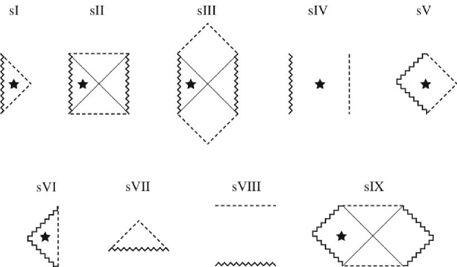
The global structure of the spacetime is characterized by properties of the singularities, horizons, and infinities. A horizon is a null hypersurface defined by such that with finite curvatures, where is a constant horizon radius. In this paper, we call a horizon on which a black hole horizon Penrose . If there is a horizon inside of a black hole horizon, and if it satisfies , we call it an inner horizon. If a horizon satisfies , and if it is the outermost horizon, we call it a cosmological horizon. We call a horizon on which a degenerate horizon. Among them, if the first non-zero derivative coefficient is positive, i.e., and for any , , we call it a degenerate black hole horizon. A solution with the degenerate horizon is called extreme. The solutions in this paper are classified into two types by horizon existence. The first is a black hole solution which has a black hole horizon. A solution which does not have a black hole horizon but has a locally naked singularity is a globally naked solution.
Since there are many parameters in our solution, such as , (or ), , , , and branches, the analysis should be performed systematically. In this paper we employ - diagrams, which are explained in Ref. TM .
III Static solutions in the Einstein-Maxwell- system
In Gauss-Bonnet gravity, two branches of the static solution appear. The minus-branch solution reduces to the solution in the Einstein-Maxwell- system in the limit of . The metric function becomes
| (17) |
On the other hand, diverges for the plus-branch solution in this limit, and there is no counterpart in the Einstein-Maxwell- system. Before proceeding to the case with the Gauss-Bonnet terms, we first summarize the spacetime structure of the static solutions described by Eqs. (9), (10), and (17) in the Einstein-Maxwell- system for comparison. Being interested in the charged solution, we assume throughout this paper.
There is a singularity at the center (). The Kretschmann invariant behaves
| (18) | |||||
around the center. The metric function is positive around the center by Eq. (17), and the tortoise coordinate defined by
| (19) |
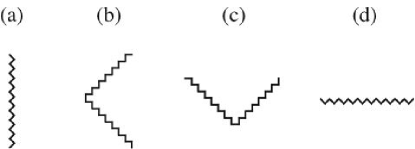
is finite at the center. Hence the singularity is always timelike (Fig. 1(a)).
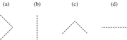
The structure of the infinity depends on the dominant term of Eq. (17) for . When there is a non-zero cosmological constant, the dominant term is . When (), the spacetime asymptotically approaches the de Sitter (dS) (anti-de Sitter (adS)) spacetime, whose region is expressed by the conformal diagram Fig. 2(d) (Fig. 2(b)). The second leading term is the curvature term . If and , the spacetime is asymptotically flat, whose region is expressed by the conformal diagram Fig. 2(a). If and , the conformal diagram of the infinity is Fig. 2(c). When , the term is dominant. For (), the infinity is expressed by Fig. 2(c) (Fig. 2(a)). When , the term is dominant, and the infinity is expressed by Fig. 2(a).
The horizon plays an important role in determining the spacetime structure. The existence of the horizon is clearly visualized on the - diagram, especially in the case where there are many parameters. By Eq. (17), the - relation in the Einstein-Maxwell- system is
| (20) |
We consider here that the values of , , and are fixed so that this relation becomes a curve on the - diagram.
From the degeneracy condition of the horizon , where is the radius of the degenerate horizon, we can show that the - curve on the diagram becomes vertical at this point. However, all the horizons at the vertical point are not necessarily degenerate. As is shown in Ref. TM , if
| (21) |
where , the horizon at the vertical point can be nondegenerate. Although this condition (21) is satisfied only if limit in general relativity, we will find below that there is no such solution. Hence the horizon at any vertical point in the Einstein-Maxwell- system is a degenerate horizon.
The mass and the charge of the extreme solution are
| (22) | |||||
| (23) |
respectively. By Eq. (23), there are extreme solutions only in the case where and/or . On the - diagram the extreme solution is expressed by the point where two horizons coincide. When is satisfied at the finite radius , the three horizons degenerate, and we call the horizon a doubly degenerate horizon.
We will examine a number of horizons of the solutions. The - diagrams are shown in Fig. 3, and the global structures are summarized in Table 1 and 2.
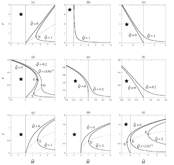
III.1 case
In the case, the solution is the -dimensional RN solution note_1 . The - diagram is shown in Fig. 3(a). For , where , the solution has no horizon and represents the spacetime with a globally naked singularity. For the solution is the -dimensional extreme RN black hole solution. The term of the square root in Eq. (24) vanishes, and a degenerate horizon locates at . For , the solution has black hole and inner horizons, which have radii with the plus and the minus signs in Eq. (24), respectively, and represents the RN black hole spacetime.
In the case, the - diagram is shown in Fig. 3(b). For the solution has no horizon and represents the spacetime with a globally naked singularity. For the solution has a cosmological horizon and represents the spacetime with a globally naked singularity.
In the case, the - diagram is shown in Fig. 3(c). The solution has a cosmological horizon for any value of and represents the spacetime with a globally naked singularity.
III.2 case
In the case, the solution is the -dimensional RN-dS solution and has three horizons at most. The - diagram is shown in Fig. 3(d).
When the charge of the solution is not as large as , there are two vertical points in the - diagram. Here is the charge of the solution with a doubly degenerate horizon
| (26) | |||
| (27) |
These vertical point E’s in Fig. 3(d) correspond to two degenerate horizons with radii and () calculated by solving Eq. (23) with respect to , respectively. The former is realized by the degeneracy of the black hole and the inner horizons, while the latter is realized by the degeneracy of the black hole and the cosmological horizons. We denote the mass of these solutions by and (), respectively. For , the solution has a cosmological horizon and represents the spacetime with a globally naked singularity. For , the solution has a degenerate black hole horizon and a cosmological horizon and represents the extreme RN-dS black hole spacetime. For , the solution has inner, black hole, and cosmological horizons. The spacetime is the RN-dS black hole spacetime. For , the solution has inner and degenerate horizons. For , the solution has a cosmological horizon and represents the spacetime with a globally naked singularity.
When , there is a solution with a doubly degenerate horizon whose mass parameter is
| (28) |
The doubly degenerate horizon locates at . This solution represents the spacetime with a globally naked singularity. The ratio of the charge to the mass is
| (29) |
The ratio takes the largest value for . For , the solution has a cosmological horizon and represents the spacetime with a globally naked singularity.
When , any solution has a cosmological horizon and represents the spacetime with a globally naked singularity.
III.3 case
The system with a negative cosmological constant have been intensively studied in the adS/CFT and braneworld contexts. Furthermore there are topological black hole solutions Brown ; Cai3 .
In the case, the solution is the RN-adS solution. The - diagram is shown in Fig. 3(g). The - diagram in the case is shown in Fig. 3(h). We can see that they have similar structures. There is one vertical point in the - diagrams. It corresponds to the degenerate horizon, whose solution has the mass and the charge calculated by Eqs. (22) and (23). The mass of both extreme solutions is positive. For , the solution has no horizon and represents the spacetime with a globally naked singularity. For , the solution has an degenerate black hole horizon and represents the extreme black hole spacetime. For , the solutions have inner and black hole horizons. The solution with represents the -dimensional RN-adS black hole spacetime.
In the case, the - diagram is shown in Fig. 3(i). The solutions are classified into three types. For , the solution has no horizons and represents the spacetime with a globally naked singularity. For , the solution has a degenerate black hole horizon and represents the extreme black hole spacetime. For , the solution has inner and black hole horizons and represents the black hole spacetime. Due to the first term in the r.h.s. of Eq. (20), a black hole solution with zero or negative mass can exist. As is seen from Fig. 3(i), the black hole solution with the lightest mass for a fixed charge is the extreme solution. When the charge is small, the extreme black hole solution has negative mass. When , where
| (30) |
the extreme black hole solution has zero mass, and its horizon radius is
| (31) |
For the charge , all the black hole solutions have positive mass.
IV General properties of solutions in the Einstein-Gauss-Bonnet-Maxwell- system
We proceed to the cases with Gauss-Bonnet terms. First, let us discuss the general properties of the static solutions in this system.
For the well-defined theory with the relevant vacuum state (), where the metric function is
| (32) |
we assume
| (33) |
For , any value of satisfies this condition while, in the negative cosmological constant case. In this and the next sections, we study the case. The special case of will be investigated in Sec. VI.
From Eq. (32), the square of the effective curvature radius is defined by
| (34) |
The sign of coincides with in the minus branch, while is always positive in the plus branch. Hence the spacetime approaches the adS spacetime asymptotically for in the plus branch for , even when the pure cosmological constant is positive. In Sec. III, we showed the structures of the infinity of the solutions, which depend on the value of , in general relativity. By replacing in the discussion in general relativity by the structures of the infinity in the Einstein-Gauss-Bonnet-Maxwell- system are obtained.
In general relativity there is a central singularity for any charged solution. In Gauss-Bonnet gravity the inside of the square root of Eq. (14) vanishes at the finite radius , and the other type of singularity, called the branch singularity, appears there. The - relation becomes
| (35) |
This relation is independent of . In the neutral case , the branch singularity appears only for the solution with negative mass TM , while all the solutions have branch singularity in the charged case. Around the branch singularity the Kretschmann invariant behaves as
| (36) |
From the condition (33), decreases monotonically as increases and asymptotically approaches zero in the limit of . It is noted that the divergent behavior of the branch singularity is milder than that of the central singularity in general relativity (see Eqs. (18) and (36)).
The metric function behaves around the branch singularity as
Hence when or , the singularity is timelike (Fig. 1(a)). When , the singularities are timelike and spacelike (Fig. 1(d)) for and , respectively. In the special case of and , the singularities are spacelike and timelike for the minus and plus branches, respectively.
On the horizon the metric function vanishes: , and we find
| (38) |
where the signs in the l.h.s. represents the minus/plus branches. Hence
| (39) | |||
| (40) |
By these condition it is concluded that there is no horizon for in the plus branch. When , the horizon radius is restricted as () in the plus (minus) branch.
The - relation is
| (41) |
For this relation is same as that in general relativity (20). For the solution with has a branch singularity at where
| (42) |
This implies that the sequence of solutions is divided by the branch singularity into the plus and the minus branches in the case. It is seen that the - curve in the - diagram terminates at the - curve just at the point we call the branch point (Point B in Figs. 4 and 5). For the mass parameter with , the horizon radius is always larger than . While is always negative in the neutral case, can be zero in the charged case by tuning the charge as
| (43) |
For (), is negative (positive).
As we will see in the next section, in the - diagram of the - curve there are some vertical points. In Gauss-Bonnet gravity,
| (44) |
is finite, so that the horizons at the vertical points are degenerate except for , where the condition (21) is satisfied. However, the - curve is tangent to the - curve at the branch point, and the - curve monotonically decreases. Thus the - curve cannot be vertical at the branch point. As a result the horizons at all the vertical points are degenerate (for this analysis, see Ref. TM .)
In the extreme cases, the relations between the mass, the charge, and the horizon radius are written as
| (45) |
| (46) |
In five dimensions the last term in Eq. (46) vanishes, and the charge of the extreme solution has the same expression as that in general relativity. This implies that degenerate horizons appear at the same radius as those appearing in general relativity if we choose the same cahrge value. However, the mass of the extreme solution is different from that in general relativity. Eq. (46) is rewritten as
| (47) | |||||
The function is defined in the range . If is negative semi-definite, there is no extreme solution. If is a monotonically increasing function from zero to infinity, there is a certain mass where the solution becomes extreme for any value of . We denote the mass of the extreme solution in the plus (minus) branch as (). When more than one extreme solution exists in the same branch, we denote their mass as , , (, , ).
If is not a monotonic function, there are extremal points, which correspond to the solutions with a doubly degenerate horizon. We should take care not to confuse these extremal points of the function with the extremal solution with degenerate horizons.
Although there may be a horizon with more degeneracy in general, in the present system up to doubly degenerate horizon can appear. Hence examining the extremal points of , we find the condition and location of the doubly degenerate horizon such that . As the charge is varied, the number of the roots in Eq. (47) changes at the extremal points of the function . When , the doubly degenerate horizon appears at
| (48) |
Since the l.h.s. of this equation is positive, must be and . Furthermore since , the doubly degenerate horizon exists only in the plus branch. Then the mass and the charge of the solution is given by Eqs. (45) and (47) as
| (49) | |||
| (50) |
When , the doubly degenerate horizon appears at
| (51) |
and the mass and the charge of the solution become
| (52) | |||
where
| (54) |
Note that the sign does not correspond to the signs of the solution branches but is determined to make the r.h.s. of Eq. (51) positive. If both signs give negative , there are two sets of parameters which give the solutions with a doubly degenerate horizon. When is single valued (namely, there is only one value of the charge which gives a doubly degenerate horizon), two extreme solutions exist for , while no extreme solution exists for .
V - diagram and spacetime structure
In the previous section, we discussed properties of the singularity, the infinity, and the horizons of the solutions in the Einstein-Gauss-Bonnet-Maxwell- system. In this section we focus on the number of horizons and show the spacetime structures by taking into account the above properties. To clarify our considerations, the - diagrams are shown in Figs. 4 () and 5 (). The spacetime structures of the solutions are summarized in Tables 2-4.
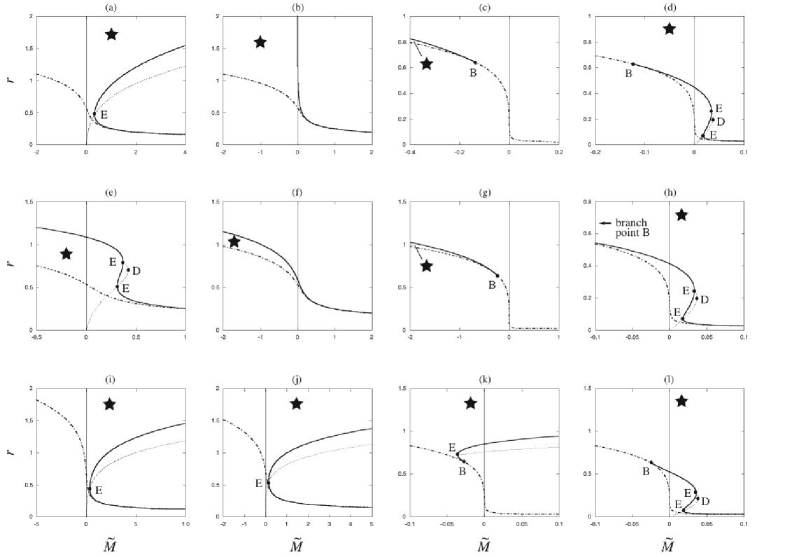
V.1
V.1.1 case
The solution in the plus branch does not have a horizon and represents the spacetime with a globally naked singularity.
The - diagrams of the minus-branch solutions are shown in Figs. 4(a) () and 5(a) (). Since the function monotonically increases from zero to infinity, there is an extreme solution for any . The extreme solution has the positive mass . For , the solution has no horizon and represents the spacetime with a globally naked singularity. For , the solution has a degenerate horizon and represents the extreme black hole spacetime. In the five-dimensional case, the mass and the horizon radius of the extreme black hole are and , respectively. For , the solution has inner and black hole horizons and represents the black hole spacetime.
V.1.2 case
The solution in the plus branch does not have a horizon and represents the spacetime with a globally naked singularity.
The - diagrams of the minus-branch solutions are shown in Figs. 4(b) () and 5(b) (). The - relation becomes , and the horizon radius diverges in the limit. For , the solution has no horizon and represents the spacetime with a globally naked singularity. For , the solution has a cosmological horizon and represents the spacetime with a globally naked singularity.
V.1.3 case
In the case, solutions in the plus branch can have horizons. Since the function has a positive maximum in the case, there is a solution with a doubly degenerate horizon when , which is given by Eqs. (48) and (50). This solution belongs to the plus branch since . When , Eq. (47) has two roots, i.e., two types of degenerate horizons exist. Since the function becomes positive for the range in this case, these extreme solutions also belong to the plus branch. The mass of these extreme solutions is denoted as and , where , respectively. On the other hand, the function is negative semi-definite in , and there is no extreme solution.
Let us first consider the solutions in the minus branch. The - diagrams of the minus-branch solutions are shown in Figs. 4(c) () and 5(c) (). The diagrams in and higher-dimensional cases are qualitatively the same. For , the solution has a cosmological horizon and represents the spacetime with a globally naked singularity. For , the solution has no horizon, and represents the spacetime with a globally naked singularity. Here is positive (negative) when (), where is given by Eq. (43) as
| (55) |
In the case, the - diagram of the plus branch solutions is shown in Fig. 4(d). The configuration of the - curve changes qualitatively depending on the value of the charge. First we assume . Then there are two extreme solutions. For , the solution has no horizon and represents the spacetime with a globally naked singularity. For , the solution has a black hole horizon and represents the black hole spacetime. Since by Eqs. (50) and (55), is negative. So, the solution with represents the negative mass black hole. For , the solution has a degenerate and a black hole horizon and represents the black hole spacetime. For , the solution has three horizons. Although the RN-dS black hole solution in general relativity also has three horizons, the global structure of the present solution differs from it. By our definition the outermost and the innermost horizons of the three horizons are the black hole horizon, i.e., there are two black hole horizons, and the horizon between them is the inner horizon. For an observer locating in the untrapped region between the “inner” black hole horizon, i.e., the innermost horizon, and the inner horizon, the inner horizon would be seen as if it were the cosmological horizon. For , the solution has a black hole and a degenerate black hole horizon and represents the extreme black hole spacetime. For , the solution has a black hole horizon and represents the black hole spacetime.
When , there is a solution with a doubly degenerate horizon. For , the solution has no horizon and represents the spacetime with a globally naked singularity. For , the solution has a black hole horizon and represents the black hole spacetime. The solution with represents the negative mass black hole. For , where is given by Eqs. (48) and (49), the solution has a doubly degenerate horizon. In general relativity, there is a solution with a doubly degenerate horizon as a special case of the RN-dS solution, as shown in Sec. III.2. That is not a black hole solution; while the present solution in Gauss-Bonnet gravity represents the black hole spacetime with a doubly degenerate horizon. The ratio of the charge to the mass becomes
| (56) |
For , the solution has a black hole horizon and represents the black hole spacetime.
When , no extreme solution exists. For , the solution has no horizon and represents the spacetime with a globally naked singularity. For , the solution has a black hole horizon and represents the black hole spacetime. If , the solution with represents the negative mass black hole.
In the case, the - diagram of the plus branch solutions is shown in Fig. 5(d). The qualitative behavior of the solutions in the minus branch is similar to that in the case, while that in the plus branch is a little different. Since the function is negative semi-definite in the case, there in no extreme solution. Hence, in the plus branch, for , the solution has no horizon and represents the spacetime with a globally naked singularity. For , the solution has a black hole horizon and represents the black hole spacetime. If , the solution with represents the negative mass black hole.
V.2
V.2.1 case
The solution in the plus branch has no horizon and represents the spacetime with a globally naked singularity. On the other hand all the solutions in the minus branch have horizons. The number of horizons depends on the charge and the mass.
The - diagrams of the minus-branch solutions are shown in Figs. 4(e) () and 5(e) (). Since the function has the positive maximum, there is a solution with a doubly degenerate horizon, whose mass and charge are given by Eqs. (IV) and (IV), respectively. When , two types of extreme solutions exist whose mass is and . For , the solution has a cosmological horizon and represents the spacetime with a globally naked singularity. For , the solution has a degenerate black hole horizon and a cosmological horizon and represents the extreme black hole spacetime. For , the solution has three horizons, which are inner, black hole and comsological horizons. The solution represents the black hole spacetime. For , the solution has an inner horizon and a degenerate horizon and represents the spacetime with a globally naked singularity. For , the solution has a cosmological horizon and represents the spacetime with a globally naked singularity.
When , there is a solution with a doubly degenerate horizon. For , the solution has a cosmological horizon and represents the spacetime with a globally naked singularity. For , the solution has a doubly degenerate horizon and represents the spacetime with a globally naked singularity.
When , no extreme solution exists. All the solutions have a cosmological horizon only and represent the spacetime with a globally naked singularity.
V.2.2 case
Since there is no horizon for the solution in the plus branch, all the solutions represent the spacetime with a globally naked singularity.
V.2.3 case
The - diagrams are shown in Figs. 4(g) (, minus branch), 4(h) (, plus branch), 5(g) (, minus branch), and 5(h) (, plus branch). The properties of the - relations are the same as those in the and case qualitatively. In the minus branch, however, the structure of the infinity is different (See the conformal diagrams).
In the case of the plus branch with and , is always less than for and , as is seen in Sec. V.1. This is also true in the present case. By the - relation (35), is a monotonically decreasing function of , and the horizon radius of the plus-branch solution is restricted as . By these facts the mass of the solution which has a horizon should be greater than . As a result, is obtained. This also holds in the case.
Although it is difficult to show analytically, we can show by comparing Eq. (IV) with Eq. (43) in the , , and limits. This supports the argument that this relation should hold for any and . Actually the numerical calculation shows . This implies that the negative mass black hole solution always exists for .
V.3
V.3.1 case
The solution in the plus branch has no horizon and represents the spacetime with a globally naked singularity.
The - diagrams of the minus-branch solutions are shown in Figs. 4(i) () and 5(i) (). Since the function monotonically increases from zero to infinity, there is an extreme solution for any . The extreme solution has the positive mass in the case and in the case. For , the solution has no horizon and represents the spacetime with a globally naked singularity. For , the solution has a degenerate black hole horizon and represents the extreme black hole spacetime. For , the solution has an inner and a black hole horizon and represents the black hole spacetime.
V.3.2 case
The solution in the plus branch has no horizon and represents the spacetime with a globally naked singularity.
V.3.3 case
In the function has two extrema. However, becomes negative for the minus sign in Eq. (54), and eventually there is one extreme solution with a doubly degenerate horizon. The value of the charge of the extreme solution is determined by Eq. (IV), where the plus sign is chosen in Eq. (54). When , Eq. (47) has three roots, and there are three extreme solutions. One of them has a degenerate horizon whose radius is large than and belongs to the minus branch. The other belong to the plus branch. When , the degenerate horizons in the plus branch coincide and become a doubly degenerate horizon. There is an extreme solution in each branch. When , there is one extreme solution only in the minus branch. In the case, there is only one extreme solution for fixed by Eq. (47). The radius of the degenerate horizon is , and the extreme solution belongs to the minus branch.
First let us consider the minus branch. The - diagrams are shown in Figs. 4(k) () and 5(k) (). For any value of , there is an extreme solution with . For , the solution has no horizon and represents the spacetime with a globally naked singularity. For , the solution has a degenerate horizon and represents the extreme black hole spacetime. For , the solution has an inner and a black hole horizon and represents the black hole spacetime. For , the solution has a black hole horizon and represents the black hole spacetime.
We plot the - curve on the - diagrams. For a small charge value, the extreme black hole solution has negative mass (the dot E in Figs. 4(k) and 5(k)). As the charge becomes large, the mass of the extreme black hole solution increases and becomes zero. We denote the charge of the zero mass extreme solution . Then when , the mass of the extreme black hole solution is negative, and the solution with represents the black hole spacetime with the negative mass. When , the extreme solution represents the zero mass black hole spacetime. When , all the black hole solutions have the positive mass.
We have seen that several extreme solutions appear in Gauss-Bonnet gravity. However, all of them do not have zero mass except for the one in the case of , in the plus branch. Let us examine this situation and derive the explicit form of . By the condition (we assume ), Eq. (45) gives
| (57) |
For ,
| (58) |
which implies that only the case can have a positive real root. However, then the is estimated by Eq. (46) as
| (59) |
which gives a contradiction so that is not defined in the case.
For , the roots of Eq. (57) are
| (60) |
The value inside of the square root is guaranteed to be positive definite by the condition (33). For there is no positive root. Substituting Eq. (60) into the Eq. (46),
| (61) |
When the r.h.s is negative definite. Hence only in the case can be defined. Moreover for , Eq. (61) gives a condition
| (62) |
which implies that the extreme solution with zero mass appears only in the minus branch. Substituting Eq. (60) into this condition in the case, one easily finds , which contradicts the condition (33). In the case, taking the lower (minus sign) solution of Eq. (60), one finds a similar contradiction. As a result, only in the and case can we define in the minus branch by taking the upper solution of Eq. (60). Its value is
| (63) |
where
| (64) |
Next let us move onto the plus branch. The - diagrams of the plus-branch solutions are shown in Figs. 4(l) () and 5(l) (). The configuration of the - diagrams are qualitatively the same as those in the , case, respectively.
In the and case, holds for any case. In the case, however, can be larger than . This can be seen easily as follows. In the limit,
| (65) | |||
| (66) |
So in this limit, . On the other hand, in the limit, and . Hence . Therefore there is a certain value of where the and are equal. also vanishes in the limit. Hence for a small , there are two extreme solutions in the plus branch for small . Simultaneously the negative mass black hole solution exists. As the charge becomes large, extreme solutions disappear while the negative mass black hole solution remains. In the large limit, however, the negative mass black hole solutions disappear, although the extreme solutions exist. These behaviors in the space of the solutions are interesting in the context of our discussion of the evolution of the black hole.
VI Einstein-Gauss-Bonnet-Maxwell- system: case
The system with is a special case, where the vacuum states of the plus and the minus branches coincide. Since we have assumed that is positive, the cosmological constant is negative by definition. The metric function becomes
| (67) |
When the radius is large the spacetime approaches adS spacetime for with the effective curvature radius for .
In the charged case, a branch singularity locates at
| (68) |
Hence the mass must be positive in this special case. There is no negative mass black hole solution. Furthermore the is independent of the Gauss-Bonnet coefficient . The Kretschmann invariant behaves as
| (69) |
around the branch singularity. Since behaves
| (70) |
near the branch singularity, the branch singularities are timelike (Fig. 1(a)) for the solutions with . For the solutions with , the singularity is timelike for and spacelike (Fig. 1(d)) for . In the special case of , the singularity is spacelike in the minus branch and timelike in the plus branch.
Since the radius of a horizon is restricted to () for the plus (minus) branch, there are no horizons for solutions with in the plus branch. The - relation (41) becomes
| (71) |
As in the case, a vertical point of the - curve corresponds to a degenerate horizon. From the condition , the relations between the mass, the charge, and the radius of the degenerate horizon of the extreme solution are
| (72) |
| (73) |
There is one extreme solution for any value of when since the r.h.s. of Eq. (73) monotonically increases. When and , there is also one extreme solution for any value of . Since the radius of the degenerate horizon is restricted to by Eq. (73) for the and case, the extreme solution belongs to the minus branch.
When and , the number of extreme solutions depends on . There is always one extreme solution with in the minus branch. For , where is obtained by substituting into Eq. (IV), there is an extreme solution with a doubly degenerate horizon in the plus branch. and are also obtained from Eqs. (51), (IV), and (54). For there are two (no) extreme solutions with and , where , respectively, in the plus branch.
By the above analysis, we can draw the - diagram. The solution in the plus branch has no horizon in the cases and represents the spacetime with a globally naked singularity. The - diagrams of the minus-branch solution in the cases are shown in Figs. 6(a) and 6(b), respectively. The solution only exists for the positive mass parameter. Besides this fact, the properties are the same as those in the case (see Figs. 4(i) and 4(j)). There is an extreme solution for any . For , the solution has no horizon and represents the spacetime with a globally naked singularity. For , the solution has a degenerate black hole horizon and represents the extreme black hole spacetime. For , the solution has an inner and a black hole horizon and represents the black hole spacetime.
In the case, the - diagram of the minus-branch solution is shown in Fig. 6(c). There is an extreme solution for any . For , the solution has no horizon and represents the spacetime with a globally naked singularity. For , the solution has a degenerate black hole horizon and represents the extreme black hole spacetime. For , the solution has inner and black hole horizons and represents the black hole spacetime. For , the solution has a black hole horizon and represents the black hole spacetime.
VII Conclusions and discussion
We have studied spacetime structures of the static solutions in the -dimensional Einstein-Gauss-Bonnet-Maxwell- system, where the cosmological constant is either positive, zero, or negative. We assume that the Gauss-Bonnet coefficient is non-negative. This assumption is consistent with the notion that the action is derived from superstring/M-theory in the low-energy limit. The solutions have the -dimensional Euclidean sub-manifold whose curvature is , or . We assume in order to define the relevant vacuum state. The structures of the center, horizons, infinity, and the singular point depend on the parameters of the system and the branches complicatedly so that a variety of global structures for the solution is found. In our analysis, the - diagram provides an easily understood visual clatification.
In Gauss-Bonnet gravity, the solutions are classified into plus and minus branches. In the limit, the solution in the minus branch recovers the one in general relativity, while there is no solution in the plus branch. The structure of the infinity is not determined by the cosmological constant alone but also by the effective curvature radius . In the minus branch the ordinary correspondence between the signs of the cosmological constant and the asymptotic structures is obtained. In the plus branch, however, the sign of is always positive independent of the cosmological constant, so that all the solutions have the same asymptotic structure as those in general relativity with a negative cosmological constant.
In general relativity, when one adds a charge to the Schwarzschild black hole, the inner horizon appears, and the singularity changes from spacelike to timelike. Also in Gauss-Bonnet gravity, the charge affects greatly the central region of the spacetime. In the charged solutions a singularity appears at the finite radius , which is called a branch singularity. Although in the neutral case the branch singularity appears only for the negative mass parameter, in the charged case it appears for any mass parameter. It becomes timelike or spacelike depending on the parameters. Furthermore, the Kretschmann invariant behaves as around the branch singularity. This is much milder than divergent behavior of the central singularity in general relativity . This may imply that the string effects make the singular behavior milder.
There are three types of horizon: inner, black hole, and cosmological horizons. In the cases the plus-branch solutions do not have any horizon. In the case, the radius of the horizon is restricted as () in the plus (minus) branch. The point with on the - relation is the branch point whose mass is . In the neutral case is always negative, so that there is a black hole solution with negative mass. However, in the charged case becomes zero when , and for .
Among the solutions in our analysis, the black hole solutions would be the most important. Although the - relations in the cases have qualitatively similar configurations to those in general relativity, the solution in the case is quite different. The charged black hole solution in general relativity always has an inner horizon, and the singularity is timelike. For the and cases in Gauss-Bonnet gravity, the singularity of the black hole solution is timelike, too. Most of the black hole solutions with , however, have no inner horizon so that the branch singularity of these solutions becomes spacelike. When , there are black hole solutions with zero and negative mass in the plus branch for regardless of the sign of the cosmological constant. Although there is maximum mass for the black hole solutions in the plus branch for in the neutral case, no such maximum exists in the charged case, and any positive mass solution is black hole for . A solution has three horizons at most. In general relativity, the RN-dS black hole solution has three horizons which are the inner, the black hole, and the cosmological horizons. In Gauss-Bonnet gravity, the solutions in the plus branch with and have three horizons for each cosmological constant when and . The horizons of these solutions are the “inner” black hole, the inner, and the “outer” black hole horizons. We add the words “inner” and “outer” to distinguish each black hole horizon.
We investigate the system with the special parameter separately where the vacuum states in the plus and minus branches coincide. In this case only is the positive mass solution allowed; otherwise the metric function takes a complex value.
Considering the Gauss-Bonnet effects on the CCH, we find firstly that the divergent behavior around the singularity becomes milder than that in general relativity. It is, however, difficult to eliminate the singularity completely. Secondly, most of the black hole solutions in the case have no inner horizon, and the singularity is spacelike. However, all the black hole solutions in and cases still have the timelike singularity. Furthermore since the structure of the infinity of the black hole solution with is adS-like, the spacetime is not globally hyperbolic. As a result, the Gauss-Bonnet terms do not work quite well from the cosmic censorship spirit.
Let us consider the evolution of the black hole solutions. In the RN-dS black hole spacetime in general relativity, the spacetime seems to evolve to the one with globally naked singularity by throwing some mass into the black hole such that the mass of the black hole becomes larger than that of the extreme black hole solution . However, it will not happen as discussed in Ref. Nakao . In Gauss-Bonnet gravity, the situation is quite different. In the non-extreme neutral black hole spacetime in the plus branch with , there are inner and black hole horizons without a cosmological horizon TM . When one put the mass into the black hole, the radius of black hole decreases note . If more matter is added, the black hole may evolve to the extreme black hole with finite processes and then to the spacetime with a globally naked singularity. This is a classical transition from the black hole spacetime to the one with a globally naked singularity. Next let us consider the charged case where the black hole spacetime has the “inner” black hole, and the inner and the “outer” black hole horizons. This solution exists in the plus branch for . Adding the mass to the black hole, the black hole approaches the extreme solution, and then it transits to the black hole spacetime with a smaller horizon whose mass is . This is a classical transition from one black hole spacetime to another black hole spacetime. On the other hand, another process, i.e., the Hawking evaporation process, may occur in our black hole spacetime. The black hole in this plus-branch solution may evaporate and lose its mass. Then, what happens when the mass of the black hole becomes , where the horizon inside of the “outer” black hole horizon degenerates? To obtain the precise scenario of the evolutions of black hole spacetime through classical and quantum processes, we need detailed analysis.
There are some applications and extensions of the present investigation. We find that the static solutions in Gauss-Bonnet gravity have much variety and interesting properties. One of the most important issues is stability of the solutions. There are some studies which support the dynamical stability of the exterior spacetime of the black hole solutions in Gauss-Bonnet gravity Neupane ; Dotti ; Konoplya . However, they do not cover all the cases, and there remain some uncleared analyses. The problem of the stability of the inner horizons has also been raised. This is interesting from the CCH point of view mass-inf ; kink . We find several solutions with degenerate horizons. They correspond to the solutions with product metric such as the Nariai and the Bertotti-Robinson solutions. All the solutions of this type in the Einstein-Maxwell- system have been recently classified in Ref. Lemos . It would be interesting to extend the analysis to Gauss-Bonnet gravity. Another application is to the braneworld. The solution with a negative cosmological constant and/or in the plus branch has the adS-like structure of the infinity. These solutions can be applied to the bulk spacetime of the braneworld and are currently under investigation.
Acknowledgements
We would like to thank Kei-ichi Maeda and Umpei Miyamoto for their discussion. This work was partially supported by a Grant for The 21st Century COE Program (Holistic Research and Education Center for Physics Self-Organization Systems) at Waseda University.
References
- (1) N. Arkani-Hamed, S. Dimopoulos, and G. Dvali, Phys. Lett. B 429, 263 (1998); I. Antoniadis, N. Arkani-Hamed, S. Dimopoulos, and G. Dvali, Phys. Lett. B 436, 257 (1998).
- (2) L. Randall and R. Sundrum, Phys. Rev. Lett. 83, 3370 (1999); 83, 4690 (1999).
- (3) G. Dvali, G. Gabadadze, and M. Porrati, Phys. Lett. B 485, 208 (2000); G. Dvali and G. Gabadadze, Phys. Rev. D 63, 065007 (2001); G. Dvali, G. Gabadadze, and M. Shifman, Phys. Rev. D 67, 044020 (2003).
- (4) S. Dimopoulos and G. Landsberg, Phys. Rev. Lett. 87, 161602 (2001); A. Chamblin and G.C. Nayak, Phys. Rev. D 66, 091901 (2002); S. B. Giddings and S. Thomas, Phys. Rev. D 65, 056010 (2002).
- (5) P. Hořava and E. Witten, Nucl. Phys. B475, 94 (1996); A. Lukas, B. A. Ovrut, K.S. Stelle, and D. Waldram, Phys. Rev. D 59, 086001 (1999); A. Lukas, B. A. Ovrut, and D. Waldram, Phys. Rev. D 60, 086001 (1999).
- (6) D. J. Gross and E. Witten, Nucl. Phys. B277, 1 (1986); D. J. Gross and J. H. Sloan, Nucl. Phys. B291, 41 (1987); R. R. Metsaev and A. A. Tseytlin, Phys. Lett. B 191, 354 (1987); R. C. Meyers, Phys. Rev. D 36, 392 (1987); C. G. Callan, R. C. Myers, and M. J. Perry, Nucl. Phys. B311, 673 (1988); R. R. Metsaev and A. A. Tseytlin, Nucl. Phys. B293, 385 (1987).
- (7) B. Zwieback, Phys. Lett. B 156, 315 (1985); B. Zumino, Phys. Rep. 137, 109 (1986).
- (8) Y. Choquet-Bruhat, C. R. Acad. Sci. I 306, 445 (1988); Y. Choquet-Bruhat, J. Math. Phys. 29, 1891 (1988).
- (9) T. Torii and H. Maeda, hep-th/0504127.
- (10) D. G. Boulware and S. Deser, Phys. Rev. Lett. 55, 2656 (1985).
- (11) J. T. Wheeler, Nucl. Phys. B268, 737 (1986).
- (12) See, for example, T. Torii, H. Yajima, and K. Maeda, Phys. Rev. D 55, 739 (1997) and references therein.
- (13) R. Penrose, Riv. Nuovo Cim. 1, 252 (1969).
- (14) R. Penrose, in General Relativity, an Einstein Centenary Survey, edited by S. W. Hawking and W. Israel (Cambridge University Press, Cambridge, England, 1979), p. 581.
- (15) R. Penrose, in Battelle Rencontres, edited by C. de Witt and J. A. Wheeler (W.A. Benjamin, New York, 1968), p. 222.
- (16) E. Poisson and W. Israel, Phys. Rev. D 41, 1796 (1990).
- (17) P. R. Brady, Prog. Theor. Phys. Suppl. 136, 29 (1999).
- (18) T. Harada, Pramana 63(4) (2004) 741.
- (19) J. M. Maldacena, Adv. Theor. Math. Phys. 2, 231 (1998); E. Witten, Adv. Theor. Math. Phys. 2, 253 (1998); S. Gubser, I. Klebanov, and A. Polyakov, Phys. Lett. B 428, 105 (1998); O. Aharony, S. Gubser, J. Maldacena, H. Ooguri, and Y. Oz, Phys. Rep. 323, 183 (2000).
- (20) C. Csáki, J. Erlich, and C. Grojean, Nucl Phys B604, 312 (2001).
- (21) C. W. Misner, K. S. Thorne, and J. A. Wheeler, Gravitation, (Freeman, 1973).
- (22) S. W. Hawking and G. F. R. Ellis, The large scale structure of space-time (Cambridge University Press, Cambridge, England, 1973).
- (23) In the higher-dimensional cases, the -dimensional Einstein space is not necessarily sphere or its quotient space even for positive curvature. Hence the solution represents not only the (at least locally) RN spacetime but also many others. However, we refer to all such cases together as “RN spacetimes”. In the following sections we will also follow this usage.
- (24) J. D. Brown, J. Creighton, and R. B. Mann, Phys. Rev. Lett. 50, 6394 (1984).
- (25) See references in R. -G. Cai and K. -S. Soh, Phys. Rev. D 59, 044013 (1999).
- (26) T. Chiba, K. Maeda, K. Nakao, and T. Tsukamoto Phys. Rev. D 57, 6119 (1998).
- (27) Since entropy of the black hole increases, the decrease of the area of the black hole horizons does not contradict the second law of black hole thermodynamics.
- (28) I. P. Neupane, Phys. Rev. D 69, 084011 (2004).
- (29) G. Dotti and R. J. Gleiser, Class. Quantum Grav. 22, L1 (2005).
- (30) T. Konoplya, Phys. Rev. D 71, 024038 (2005).
- (31) R. Penrose, in Battelle Rencontres, edited by C. de Witt and J. A. Wheeler (W.A. Benjamin, New York, 1968), p.222; E. Poisson and W. Israel, Phys. Rev. D 41, 1796 (1990); P. R. Brady, Prog. Theor. Phys. Suppl. 136, 29 (1999).
- (32) See also the references in H. Maeda, T. Torii, and T. Harada, Phys. Rev. D 71, 064015 (2005).
- (33) V. Cardoso, Ó. J. C. Dias, and J. P. S. Lemos, Phys. Rev. D 70, 024002 (2004).
| type | type | type | ||||
| 1 | sI | see Table 2 | sIV | |||
| dbI | dbII | |||||
| bVII | bIV | |||||
| 0 | sI | any | sII | sIV | ||
| sIII | dbII | |||||
| bIV | ||||||
| -1 | any | sIII | any | sII | sIV | |
| dbII | ||||||
| bIV | ||||||
| type | type | type | |||
|---|---|---|---|---|---|
| sII | sII | any | sII | ||
| dbIII | dsIII | ||||
| bVIII | sII | ||||
| dsII | |||||
| sII | |||||
| , ( branch) | , ( branch) | , ( branch) | branch | |||||
| type | type | type | type | |||||
| 1 | sI | see Table 2 | sIV | any | sIV | |||
| dbI | dbII | |||||||
| bVII | bIV | |||||||
| 0 | sI | any | sII | sIV | any | sIV | ||
| sIII | dbII | |||||||
| bIV | ||||||||
| -1 | sIII | sII | sIV | see Table 4 | ||||
| sVII | sVIII | dbII | ||||||
| bIV | ||||||||
| bIII | ||||||||
| type | type | type | type | ||||
|---|---|---|---|---|---|---|---|
| sIV | sIV | sIV | sIV | ||||
| bIII | bIII | bIII | bIII | ||||
| dbV | dbIV | ||||||
| bVI | bIII | ||||||
| dbVII | |||||||
| bIII | |||||||
| branch | branch | |||
| type | type | |||
| 1, 0 | sIV | sIV | ||
| dbII | ||||
| bIV | ||||
| -1 | sIV | see Table 4 | ||
| dbII | (The range is | |||
| bIV | changed to .) | |||
| bIII | ||||