Cosmic acceleration from M theory on twisted spaces

Ishwaree P. Neupane ishwaree.neupane@canterbury.ac.nz    David L. Wiltshire david.wiltshire@canterbury.ac.nz Department of Physics and Astronomy, University of Canterbury, Private Bag 4800, Christchurch, New Zealand
Abstract

In a recent paper [I. P. Neupane and D. L. Wiltshire, Phys. Lett. B 619, 201 (2005).] we have found a new class of accelerating cosmologies arising from a time–dependent compactification of classical supergravity on product spaces that include one or more geometric twists along with non-trivial curved internal spaces. With such effects, a scalar potential can have a local minimum with positive vacuum energy. The existence of such a minimum generically predicts a period of accelerated expansion in the four-dimensional Einstein-conformal frame. Here we extend our knowledge of these cosmological solutions by presenting new examples and discuss the properties of the solutions in a more general setting. We also relate the known (asymptotic) solutions for multi-scalar fields with exponential potentials to the accelerating solutions arising from simple (or twisted) product spaces for internal manifolds.

pacs:
98.80.Cq, 11.25.Mj, 11.25.Yb; 98.80.Jk   [Report: hep-th/0504135]

I Introduction

The possibility that fundamental scalar fields which are uniform in space play a preeminent role on cosmological scales has been confirmed by a decade of observations. Most recently the WMAP measurements of fine details of the power spectrum of cosmic microwave background anisotropies wmap have lent strong support to the idea that the universe underwent an early inflationary expansion at high energy scales. The WMAP data, along with the independent observations of the dimming of type Ia supernovae in distant galaxies Riessetal99 are also usually interpreted as an indication that the universe is undergoing accelerated expansion at the present epoch, albeit at a vastly lower rate.

As in the case of the much earlier period of early universe inflation, the most natural explanation for the repulsive force responsible for accelerating cosmologies would be a fundamental vacuum energy, possibly in the form of one or more dynamical homogeneous isotropic scalar fields. The nature of this dark energy, which constitutes of order 70% of the matter–energy content of the Universe at the present epoch, constitutes a mystery whose explanation is possibly the greatest challenge faced by the current generation of cosmologists.

In the $\Lambda$CDM model, the dark energy at the present epoch is attributed purely to a constant vacuum energy (or cosmological constant), or equivalently a homogeneous isotropic fluid whose pressure, $p$, and energy density, $\rho$, are related by $\rho=-p=\Lambda$. This is only the simplest (and perhaps most common) explanation. From a field theoretic viewpoint it would be perhaps more natural to attribute the dark energy to one or more dynamical scalar fields early_quintessence ; qreview . Many such quintessence models have been studied, with scalar potentials which range from completely ad hoc ones to those with various theoretical motivations. Such motivations are often more than not phenomenological. For example, ultra light pseudo Nambu–Goldstone bosons can give realistic cosmologies pngb , even if one does not specify exactly what fundamental theory such scalars belong to.

Fundamental scalar fields are of course abundant in higher–dimensional theories of gravity. The typical scalar potentials that one obtains by dimensional reduction, namely exponential potentials have been widely studied halliwell but generally without regard to the restrictions on the sign of the potential and magnitude of the coupling constants that arise from compactifications or the higher–dimensional geometry. In the case of multiple scalar fields, for example, attention has been focused on simplified potentials in which each scalar appears only once  Ed99a ; Lidsey:1992ak ; Barreiro:1999zs ; Heard:2002dr ; Guo:2003rs .

A number of models with a fundamental higher–dimensional origin, which accommodate a 4–dimensional universe with accelerating expansion have been studied over the past two decades acc_uni1 ; Litterio ; acc_uni2 , usually in relation to inflationary epochs in the very early universe. A general feature of these models was the presence of additional degrees of freedom, such as fluxes or a cosmological term. Until relatively recently it was not believed that one could obtain accelerating universes in the Einstein frame in four dimensions by compactification of pure Einstein gravity in higher dimensions Levin . In fact, the result was elevated to the status of a no–go theorem nogo1 .

Townsend and Wohlfarth TW circumvented the no–go theorem by relaxing its conditions to obtain time-dependent (cosmological) compactifications of pure Einstein gravity in arbitrary dimensions, with negatively curved internal space, which are made compact by topological identifications. Their exact solutions exhibit a transient epoch of acceleration between decelerating epochs at early and late times, albeit with the number of e-folds of order unity. Applied to late–time cosmologies, this could mean that our present cosmic acceleration is not eternal but switches off in a natural way.

Transient acceleration was subsequently shown to be a generic feature of many supergravity compactifications CMChen:2002 ; OhtaPRL03 ; MNR03a ; Emparan03a ; CHNW03b ; CHNOW03b ; Roy:2003nd ; Wohlfarth:2003kw ; Townsend03b ; IPN03c ; IPN03d , some models including higher–dimensional fluxes appropriate to particular supergravity models, and others with more complicated internal product spaces with negatively curved factors. The generic nature of transient acceleration is understood also for some simple potentials arising from group manifold reductions Bergshoeff:2003vb , and a compactification of M–theory on a singular Calabi-Yau space Jarv:2003qy . All these solutions typically exhibit a short period of accelerated expansion. Other approaches to accelerating cosmologies involve Maeda:2004hu a compactification of string/M theory with higher order curvature corrections, such as $(\mbox{Weyl})^{4}$ terms in type II string theory, see also a review Ohta:2004wk . In this rather complicated scenario, the analysis is often restricted to asymptotic solutions of the evolution equations, which involve a fine-tuning of the string coupling or the Planck scale in the higher dimensions (10 or 11). It is not immediately clear if any asymptotic solutions would be available within the full string theories.

In a recent paper IshDavid05 we have found a new class of supergravity cosmologies arising from time–dependent compactifications of pure Einstein gravity, whose existence is somewhat counter to the intuition of Ref. TW . In particular, we have exhibited exact solutions which circumvent the no–go theorem nogo1 , while retaining Ricci–flat internal spaces. This is possible through the introduction of one or more geometric twists in the compact space. The observation that acceleration is possible even for Ricci-flat cosmological compactifications is not new, which only required the introduction of external fluxes or form-fields OhtaPRL03 ; Emparan03a ; IPN03d . Our approach in IshDavid05 was different in the regard that acceleration is possible even if all available eternal fluxes are turned-off: in a sense, the effect of form-fields is replaced by a non-trivial “twist” in the internal geometry. Here we considerably extend our knowledge of these solutions by presenting new examples, and discuss their properties in a more general setting.

The rest of the paper is organized as follow. In Sec. II, we review the product space compactification and further discuss solutions to the vacuum Einstein equations where the internal product space involves one or more geometric twists, or alternatively some non-trivial curved internal spaces. We examine these cosmological solutions broadly into three categories: (i) a geometric twist alone; (ii) a non-trivial curvature alone, and (iii) a combination of both. In the last case, (iii), we will adopt a different gauge to solve the equations fully.

In Sec. III, we discuss the cosmology on product spaces by using the effective four-dimensional scalars which parameterize the radii of the internal spaces and show that when the internal space includes one or more twists along with non-flat extra dimensions, then a scalar potential arising from a cosmological compactification possesses a local (de Sitter) minimum, whose existence generically predicts a period of accelerated expansion in the four-dimensional Einstein conformal frame. In Sec. IV, we discuss the properties of the effective potential in a more general setting, which relate our solutions to the solutions given in literature in the context of canonical 4d gravity coupled with multiple scalars in an exponential form. In Sec. V, we will present more new examples where the physical 3-space expands faster than the internal space.

II Product space compactification: Basic Equations

The interest in time-dependent supergravity (or S-branes CMChen:2002 ) solutions arises mainly from the relation of this system to string/M–theory and from a ‘no-go’ theorem nogo1 which applies if one does not consider cosmological solution. In fact, the physical three space dimensions as ordinarily perceived are intrinsically time dependent, and if the fundamental description of nature would involve 6 or 7 (hidden) extra dimensions of space, as is required for string/M theory to work, then it is reasonable to assume that the internal space is also time dependent. We therefore consider model cosmologies described by a general metric ansatz in the following form:

$\displaystyle{\rm d}s_{4+n}^{2}=e^{-2\Phi}{\rm d}s_{4}^{2}+\sum_{i}r_{i}^{2}\,e^{2\phi_{i}}{\rm d}\Sigma^{2}_{m_{i},\epsilon_{i}},$ (1)

where the parameters $r_{i}$ define appropriate curvature radii, and ${\rm d}s_{4}^{2}$ is the metric of the physical large dimensions in the form

$${\rm d}s_{4}^{2}=-{a(u)}^{2\delta}{{\rm d}u}^{2}+{a(u)}^{2}{\rm d}\Omega^{2}_{k,3},$$ (2)

so that $\phi=\phi(u)$. Here $\delta$ is a constant, the choice of which fixes the nature of the time coordinate, $u$, and ${\rm d}\Sigma^{2}_{m_{i},\epsilon_{i}}$ are the metrics associated with $m_{i}$-dimensional Einstein spaces; the values of $\epsilon_{i}=0,\,+1,\,-1$ correspond to the flat, spherical, or hyperbolic spaces, respectively.

For the metric (1), the Einstein-Hilbert action is

$\displaystyle I$ $\displaystyle=$ $\displaystyle\frac{1}{16\pi G_{4+n}}\int d^{4+n}x\sqrt{-g}R$ (3)
$\displaystyle=$ $\displaystyle\frac{1}{16\pi G_{4+n}}\int d^{n}x\sqrt{g_{n}}\int d^{4}x\sqrt{-g_{4}}{\rm e}^{-4\Phi}{\rm e}^{\sum_{i}m_{i}\phi_{i}}\left[\frac{R_{4}}{{\rm e}^{-2\Phi}}+\sum_{i}\frac{R_{m_{i}}}{{\rm e}^{2\phi_{i}}}+\cdots\right].$

where $\sum_{i}m_{i}\equiv n$. The dots denote, apart from the obvious kinetic terms for the volume moduli $\phi_{i}$, the other possible contributions to the 4d effective potential in the presence of fluxes and/or geometric twists in the extra dimensions. When the size of the internal space changes, as in the present case, since $\phi_{i}\equiv\phi_{i}(u(t))$, the effective Newton constant becomes time dependent, in general. This is however not preferable for a model of our universe. To remedy this problem, one must choose a Einstein conformal frame in four dimensions by setting CHNW03b

$$\Phi=\frac{1}{2}\sum_{i}m_{i}\phi_{i}.$$ (4)

The Newton’s constant in four dimensions is then time–independent. With (4), the $(4+n)$ dimensional action simplifies into the sum of the 4d Einstein-Hilbert action plus an action for the scalar fields $\phi_{i}$, which determine the size of extra dimensions.

In the product space compactification case, as studied in detail in CHNW03b ; CHNOW03b , we have $m_{i}\geq 2$. However, in this paper we focus primarily in the case where some of the internal (product) spaces involve one or more geometric twists, so that $m_{i}=1$ for some $i$’s. For a mathematical simplicity we work in the gauge $\delta=3$, in (2). The $tt$- and $xx$-components of the field equations are

$\displaystyle 2K-\Phi^{\prime\prime}+3\left(\frac{a^{\prime\prime}}{a}-3\frac{{a^{\prime}}^{2}}{a^{2}}\right)=0$ (5)
$\displaystyle\Phi^{\prime\prime}+\left(\frac{a^{\prime}}{a}\right)^{2}-\frac{a^{\prime\prime}}{a}-{2k}\,{a^{4}}=0,$ (6)

where prime denotes a derivative with respect to $u$, $k$ is the spatial curvature and

$$K=\sum_{i=1}\frac{m_{i}(m_{i}+2)}{4}{\phi_{i}^{\prime}}^{2}+\sum_{i>j=1}\frac{m_{i}m_{j}}{2}{\phi_{i}}^{\prime}{\phi_{j}}^{\prime}\,.$$ (7)

In the case of compactification on symmetric spaces taken in direct products, the (scalar) field equations associated with the extra dimensions are

$$\phi_{i}^{\prime\prime}+(m_{i}-1)\sigma_{i}e^{-(m_{i}+2)\phi_{i}-\sum_{i\neq j}m_{j}\phi_{j}}a^{6}=0,$$ (8)

where $\sigma_{i}=\epsilon_{i}/r_{i}^{2}$. However, with the introduction of a geometric twist along the internal space, the field equations for $\phi_{i}$ will be modified.

To be more precise, let us consider a $(4+n)$ dimensional metric ansatz, with $n=p+2q+1$,

$${\rm d}s_{4+n}^{2}=e^{-2\Phi}{\rm d}s_{4}^{2}+r_{1}^{2}\,e^{2\phi_{1}}{\rm d}s^{2}({\cal M}^{p}_{\epsilon_{1}})+{\rm d}s_{2q+1}^{2},$$ (9)

where ${\cal M}^{p}$ is a $p$–dimensional space of constant curvature of sign $\epsilon_{1}=0,\pm 1$. The remaining $2q+1$ dimensions form a twisted product space

$${\cal M}^{2q+1}=\underbrace{{\cal M}^{2}\times{\cal M}^{2}\times\cdots\times{\cal M}^{2}}_{q~{}\text{times}}\ltimes S^{1},$$

whose metric may be given in the form

$${\rm d}s_{2q+1}^{2}=r_{2}^{2}{\rm e}^{2\phi_{2}}{\rm d}s^{2}\left({\cal M}_{\epsilon_{\lower 2.0pt\hbox{$\scriptstyle 2$}}}^{2q}\right)+r_{3}^{2}e^{2\phi_{3}}\left(dz+f\varpi_{\epsilon_{2}}\right)^{2},$$ (10)

with $f$ being the twist parameter. More specifically,

$$\vbox{\halign{&$\displaystyle#$\hfil\cr{\rm d}s^{2}({\cal M}^{2q}_{\lower 2.0pt\hbox{$\scriptstyle+1$}})&=\sum_{i=1}^{q}({\rm d}x_{i}^{2}+\sin^{2}x_{i}\,{\rm d}y_{i}^{2}),\quad\varpi_{\lower 2.0pt\hbox{$\scriptstyle+1$}}=\cos x_{i}\,dy_{i}\hfil,\cr{\rm d}s^{2}({\cal M}^{2q}_{\lower 2.0pt\hbox{$\scriptstyle 0$}})\hfil&=\sum_{i=1}^{q}({\rm d}x_{i}^{2}+{\rm d}y_{i}^{2}),\quad\varpi_{\lower 2.0pt\hbox{$\scriptstyle 0$}}=\frac{1}{2}(x_{i}dy_{i}-y_{i}dx_{i}),\cr{\rm d}s^{2}({\cal M}^{2q}_{\lower 2.0pt\hbox{$\scriptstyle-1$}})&=\sum_{i=1}^{q}({\rm d}x_{i}^{2}+\sinh^{2}x_{i}\,{\rm d}y_{i}^{2}),\quad\varpi_{\lower 2.0pt\hbox{$\scriptstyle-1$}}=\cosh x_{i}\,dy_{i}\cr}}.$$ (11)

In the gauge $\delta=3$, the field equations for the scalars, with arbitrary curvature $\epsilon_{i}$, may be given by

$\displaystyle\phi_{1}^{\prime\prime}+(p-1)\sigma_{1}{\rm e}^{-(p+2)\phi_{1}-2q\phi_{2}-\phi_{3}}a^{6}=0,$
$\displaystyle\phi_{2}^{\prime\prime}+\sigma_{2}{\rm e}^{-p\phi_{1}-2(q+1)\phi_{2}-\phi_{3}}a^{6}-2F^{2}{\rm e}^{-p\phi_{1}-2(q+2)\phi_{2}+\phi_{3}}a^{6}=0,$
$\displaystyle\phi_{3}^{\prime\prime}+{2q}F^{2}{\rm e}^{-p\phi_{1}-2(q+2)\phi_{2}+\phi_{3}}a^{6}=0,$ (12)

where $\sigma_{1}=\epsilon_{1}/r_{1}^{2}$, $\sigma_{2}=\epsilon_{2}/r_{2}^{2}$ and $F\equiv(f/2)(r_{\lower 2.0pt\hbox{$\scriptstyle 2$}}/r_{\lower 2.0pt\hbox{$\scriptstyle 3$}}^{2})$.

II.1 Compactification on symmetric spaces

Let us consider the case where $\sigma_{i}=0$ and $F^{2}=0$ (i.e. without a geometric twist). The scalar wave equations then reduce to $\phi_{i}^{\prime\prime}=0$. In this case one can easily solve the Eqs. (5),(6), with $k=0$. First consider a special case where $\phi_{1}=$const. The corresponding solution is

$$a=a_{0}{\rm e}^{c\,u},\quad\phi_{1}=\mbox{const},\quad\phi_{2}=\frac{2\sqrt{3}\,\ln{a}}{\sqrt{3\nu^{2}+{4}q(q+1+\nu)}}=\phi_{0}+\frac{\phi_{3}}{\nu},$$ (13)

where $a_{\lower 2.0pt\hbox{$\scriptstyle 0$}}$, $\phi_{0}$, $c$ and $\nu$ are constants. (Of course, the result does not depend on $p$ in this case).

For $q\gg 1$, the decompactification of some of the extra dimensions (and compactification of the other) can be a slow process. This can be seen also from the solution below, where all harmonic functions $\phi_{i}$ (or volume moduli) are time-dependent,

$$a=a_{\lower 2.0pt\hbox{$\scriptstyle 0$}}{\rm e}^{cu},\quad\phi_{3}=\mu\phi_{2},\quad\phi_{1}=\nu\phi_{2},\quad\phi_{2}=\pm\,\eta\ln{a},$$

up to a (different) shift in $\phi_{i}$, where

$$\eta\equiv\frac{2\sqrt{3}}{\sqrt{3\nu^{2}+4q(q+1+\nu)+p(p+2)\mu^{2}+p\mu(\nu+2q)}}.$$ (14)

The constants of integration $\mu,\nu,\eta$ may be chosen such that each internal space shrinks with time.

Let us briefly discuss some common features of the above solution by specializing it to a particular model with $p=4$ and $q=1$, so that

$$\Sigma_{7}=\mathbb{T}^{4}\times\mathbb{T}^{2}\times S^{1}.$$

As a particular case, let us take $\phi_{3}=-4(\phi_{1}+\phi_{2})=\phi_{0}=\text{const}$. The corresponding solution is then given by

$$a(u)=a_{0}\,e^{cu},\quad\phi_{1}=-\frac{\sqrt{3}}{2}\ln(a(u))=-(\phi_{2}+\phi_{0}/4).$$ (15)

In this example, the $2$-space $\mathbb{T}^{2}$ will grow with time, while the $4$-space $\mathbb{T}^{4}$ will shrink (or vice versa). Unfortunately, since the acceleration parameter is always negative, $\ddot{a}/a=-2c^{2}<0$ (an overdot denotes a derivative with respect to cosmic time $t$, which is defined by $t=\int a(u)^{3}{\rm d}u$), there is no acceleration in 4d Einstein conformal-frame. This all imply that there is no de Sitter (accelerating) solution in compactifications of a pure supergravity on maximally symmetric spaces of zero curvature TW . However, inclusion of a geometric twist along some of the internal (product) spaces, that is crucial to our construction below, circumvents those arguments.

II.2 The solution with a non-zero twist

Consider the case where $\sigma_{i}=0$ (or $\epsilon_{i}=0$) but $f>0$. The equations (II) then reduce to $\phi_{1}^{\prime\prime}=0$, $\phi_{3}^{\prime\prime}=-q\phi_{2}^{\prime\prime}$. We can then solve the equations (5) and (6) simultaneously. The explicit exact solution, with arbitrary values of $p$ and $q$, is given by

$\displaystyle a=a_{\lower 2.0pt\hbox{$\scriptstyle 0$}}\left(\cosh\chi(u-u_{\lower 2.0pt\hbox{$\scriptstyle 0$}})\right)^{b_{\lower 2.0pt\hbox{$\scriptstyle 0$}}}{\rm e}^{c_{\lower 2.0pt\hbox{$\scriptstyle 0$}}u},\quad\phi_{1}=\frac{2}{p}\ln\left(\frac{fr_{\lower 2.0pt\hbox{$\scriptstyle 3$}}a_{\lower 2.0pt\hbox{$\scriptstyle 0$}}^{3}}{\chi r_{\lower 2.0pt\hbox{$\scriptstyle 2$}}^{2}}\right)-c_{\lower 2.0pt\hbox{$\scriptstyle 1$}}u,$
$\displaystyle\phi_{2}=\frac{1}{2}\ln\cosh\chi(u-u_{\lower 2.0pt\hbox{$\scriptstyle 0$}})+d_{\lower 2.0pt\hbox{$\scriptstyle 0$}}u=-\frac{\phi_{3}}{q},$ (16)

where $b_{\lower 2.0pt\hbox{$\scriptstyle 0$}}\equiv q/4$,

$\displaystyle c_{\lower 2.0pt\hbox{$\scriptstyle 0$}}\equiv\frac{q(3qc+pc_{\lower 2.0pt\hbox{$\scriptstyle 1$}}+4c)}{8},\quad d_{\lower 2.0pt\hbox{$\scriptstyle 0$}}\equiv\frac{3qc+pc_{\lower 2.0pt\hbox{$\scriptstyle 1$}}}{4},\quad\chi\equiv\frac{1}{\sqrt{q}}\sqrt{8c_{\lower 2.0pt\hbox{$\scriptstyle 0$}}d_{\lower 2.0pt\hbox{$\scriptstyle 0$}}-p(p+2)c_{\lower 2.0pt\hbox{$\scriptstyle 1$}}^{2}-pqcc_{\lower 2.0pt\hbox{$\scriptstyle 1$}}}$ (17)

and $a_{0}$ and $c$ are integration constants. Note that not all constants of integration are shown: different (gauge) shifts may be taken in $\phi_{i}$; some of which can be absorbed into the $r_{i}$. The value of $u_{\lower 2.0pt\hbox{$\scriptstyle 0$}}$ is merely a gauge choice and so we set $u_{\lower 2.0pt\hbox{$\scriptstyle 0$}}=0$ henceforth. The solution (II.2) would be available even if $p=0$, in which case as there is no space ${\cal M}^{p}$, the expression for $\phi_{1}$ drops off.

The 4d cosmic time $t$ is defined by ${\rm d}t=\pm a(u)^{3}{\rm d}u$. The acceleration parameter is given by

$${a^{5}\ddot{a}}=b_{\lower 2.0pt\hbox{$\scriptstyle 0$}}\chi^{2}-2c_{\lower 2.0pt\hbox{$\scriptstyle 0$}}^{2}-4b_{\lower 2.0pt\hbox{$\scriptstyle 0$}}c_{\lower 2.0pt\hbox{$\scriptstyle 0$}}\chi\tanh\chi u-b_{\lower 2.0pt\hbox{$\scriptstyle 0$}}\chi^{2}(1+2b_{\lower 2.0pt\hbox{$\scriptstyle 0$}})\tanh^{2}\chi u,$$ (18)

where an overdot denotes differentiation w.r.t. cosmic time, $t$. It follows that solutions will exhibit a period of transient acceleration provided that

$$2c_{\lower 2.0pt\hbox{$\scriptstyle 0$}}^{2}-b_{\lower 2.0pt\hbox{$\scriptstyle 0$}}(1+2b_{\lower 2.0pt\hbox{$\scriptstyle 0$}})\chi^{2}>0.$$ (19)

Acceleration occurs on the internal $u_{-}<u<u_{+}$, where

$$\tanh\chi u_{\pm}=\frac{-2c_{\lower 2.0pt\hbox{$\scriptstyle 0$}}\pm\sqrt{\chi^{2}(1+2b_{\lower 2.0pt\hbox{$\scriptstyle 0$}})-2c_{\lower 2.0pt\hbox{$\scriptstyle 0$}}^{2}/b_{\lower 2.0pt\hbox{$\scriptstyle 0$}}}}{\chi(1+2b_{\lower 2.0pt\hbox{$\scriptstyle 0$}})}.$$ (20)

The number of e–folds during the (transient) period of acceleration, $N_{e}\equiv\ln\,a(u_{+})-\ln\,a(u_{-})$ is given by

$$N_{e}=\frac{b_{\lower 2.0pt\hbox{$\scriptstyle 0$}}}{2}\ln\left[\left(\frac{1+\tanh\chi u_{+}}{1+\tanh\chi u_{-}}\right)^{\kappa-1}\left(\frac{1-\tanh\chi u_{-}}{1-\tanh\chi u_{+}}\right)^{\kappa+1}\right].$$ (21)

where $\kappa\equiv c_{\lower 2.0pt\hbox{$\scriptstyle 0$}}/(\chi b_{\lower 2.0pt\hbox{$\scriptstyle 0$}})$. To the parameters given in (17), one has $\kappa\equiv((3q+4)c+p\,c_{\lower 2.0pt\hbox{$\scriptstyle 1$}})/{2\chi}$. The number of e–folds $N_{e}$ reaches a maximum when $c_{\lower 2.0pt\hbox{$\scriptstyle 1$}}=0$, or equivalently $\kappa=\sqrt{3q+4\over 3q}$, independently of $p$. This reflects the fact that the $c_{\lower 2.0pt\hbox{$\scriptstyle 1$}}=0$ solution is formally equivalent to the $p=0$ solution with no ${\cal M}^{p}$ torus and just the twisted $(2q+1)$–dimensional space as an internal space. One may show that the maximum number of e–folds is therefore given analytically by

$$(N_{e})_{\hbox{\sevenrm max}}=\frac{q}{8}\ln\left\{\left((q+2)\sqrt{3}+2-\sqrt{q(3q+4)}\over(q+2)\sqrt{3}-2-\sqrt{q(3q+4)}\right)^{\sqrt{3q+4\over 3q}-1}\left((q+2)\sqrt{3}+2+\sqrt{q(3q+4)}\over(q+2)\sqrt{3}-2+\sqrt{q(3q+4)}\right)^{\sqrt{3q+4\over 3q}+1}\right\}.$$ (22)

The number of e-folds increases only marginally when $q$ is increased.

Let us first briefly discuss some common features of the $f>0$ solution by setting $q=2$, so that

$$b_{\lower 2.0pt\hbox{$\scriptstyle 0$}}=1/2,\quad c_{\lower 2.0pt\hbox{$\scriptstyle 0$}}=(10c+pc_{\lower 2.0pt\hbox{$\scriptstyle 1$}})/{4}=d_{\lower 2.0pt\hbox{$\scriptstyle 0$}}+c,\quad\chi=\sqrt{15c^{2}+3pcc_{\lower 2.0pt\hbox{$\scriptstyle 1$}}-p(4+p)c_{1}^{2}/4}.$$ (23)

The solution will then exhibit a period of transient acceleration provided that $\alpha_{\lower 2.0pt\hbox{$\scriptstyle 2-$}}c<c_{\lower 2.0pt\hbox{$\scriptstyle 1$}}<\alpha_{\lower 2.0pt\hbox{$\scriptstyle 2+$}}c$, where

$$\alpha_{\lower 2.0pt\hbox{$\scriptstyle 2\pm$}}=\frac{2p\pm 4\sqrt{2p(2p+5)}}{p(3p+8)}.$$ (24)

This implies, e.g. when $p=2$, $-\frac{5}{7}c<c_{1}<c$. Acceleration occurs on the internal $|u_{-}|<u<|u_{+}|$ where

$$\tanh(\chi u_{\pm})=\frac{-\kappa\pm\sqrt{2-\kappa^{2}}}{2},$$ (25)

and $\kappa\equiv(10c+pc_{\lower 2.0pt\hbox{$\scriptstyle 1$}})/2\chi$. The volume moduli associated with ($\mathbb{T}^{2}\times\mathbb{T}^{2})\ltimes S^{1}$ are stabilized at late times when

$$c_{1}=\pm\frac{6c}{\sqrt{3p(p+2)}}.$$

For $p=2$, this yields $c_{1}=\pm\sqrt{\frac{3}{2}}c$, which lies outside the range that is required for acceleration. In the above example, the extra dimensions cannot be stabilized completely, if there is to exist a period of acceleration in the four-dimensional Einstein conformal frame.

II.3 Solutions with flat and hyperbolic extra dimensions

In this subsection we focus primarily on solutions that are obtained from compactifications on a product of hyperbolic and flat spaces. In fact, in the $F^{2}=0$ case, to have a positive potential we need to compactify a higher dimensional gravitational theory on spaces that include, at least, one negatively curved factor TW ; CHNOW03b . Here we can make the problem simpler by considering that (i) the $p$ dimensional space ${\cal M}^{p}$ is negatively curved while the $2q$-space ${\cal M}^{2q}={\cal M}^{2}\times\cdots\times{\cal M}^{2}$ is Ricci flat (${\cal M}^{2}=\mathbb{T}^{2}$) (case I) or (ii) ${\cal M}^{p}$ is Ricci flat and ${\cal M}^{2q}$ is negatively curved (${\cal M}^{2}=\mathbb{H}^{2}$) (case II).

In the first case, the solution is given by

$\displaystyle a(u)=\frac{{\rm e}^{c_{\lower 2.0pt\hbox{$\scriptstyle 0$}}u}}{\left(\sinh\chi{|u|}\right)^{b_{\lower 2.0pt\hbox{$\scriptstyle 0$}}}},\quad\phi_{1}=c_{\lower 2.0pt\hbox{$\scriptstyle 1$}}{u}-\frac{1}{(p-1)}\ln\sinh\chi{|u|},$ (26)
$\displaystyle\phi_{2}=c_{\lower 2.0pt\hbox{$\scriptstyle 2$}}{u},\quad\phi_{3}=c_{\lower 2.0pt\hbox{$\scriptstyle 3$}}{u}+2\ln\left(\frac{p-1}{\chi r_{\lower 2.0pt\hbox{$\scriptstyle 1$}}}\right),$

where $b_{\lower 2.0pt\hbox{$\scriptstyle 0$}}\equiv p/[2(p-1)]$ and

$\displaystyle c_{\lower 2.0pt\hbox{$\scriptstyle 0$}}\equiv\frac{p((p+2)c+2qc_{\lower 2.0pt\hbox{$\scriptstyle 2$}}+c_{\lower 2.0pt\hbox{$\scriptstyle 3$}})}{4(p-1)},\quad c_{\lower 2.0pt\hbox{$\scriptstyle 1$}}\equiv\frac{3cp+2qc_{\lower 2.0pt\hbox{$\scriptstyle 2$}}+c_{\lower 2.0pt\hbox{$\scriptstyle 3$}}}{2(p-1)},$
$\displaystyle\chi^{2}=\frac{1}{4p}\left[4qc_{\lower 2.0pt\hbox{$\scriptstyle 2$}}(3p-2)(c_{\lower 2.0pt\hbox{$\scriptstyle 3$}}+c_{\lower 2.0pt\hbox{$\scriptstyle 2$}}q)+8q(p-1)c_{\lower 2.0pt\hbox{$\scriptstyle 2$}}^{2}+(7p-6)c_{\lower 2.0pt\hbox{$\scriptstyle 3$}}^{2}+3p^{2}\left((p+2)c^{2}+4qcc_{\lower 2.0pt\hbox{$\scriptstyle 2$}}+2cc_{\lower 2.0pt\hbox{$\scriptstyle 3$}}\right)\right],$ (27)

with $c$ being an arbitrary constant.

In the second case, the explicit solution is

$\displaystyle a(u)=\frac{{\rm e}^{c_{\lower 2.0pt\hbox{$\scriptstyle 0$}}u}}{\left(\sinh\chi{|u|}\right)^{b_{\lower 2.0pt\hbox{$\scriptstyle 0$}}}},\quad\phi_{1}=c_{\lower 2.0pt\hbox{$\scriptstyle 1$}}{u},\quad\phi_{2}={c_{\lower 2.0pt\hbox{$\scriptstyle 2$}}}{u}-\frac{1}{2q-1}\ln\sinh\chi{|u|},$
$\displaystyle\phi_{3}=c_{\lower 2.0pt\hbox{$\scriptstyle 3$}}{u}+2\ln\left(\frac{\sqrt{2q-1}}{\chi r_{\lower 2.0pt\hbox{$\scriptstyle 2$}}}\right),$ (28)

where $b_{\lower 2.0pt\hbox{$\scriptstyle 0$}}\equiv q/(2q-1)$ and

$\displaystyle c_{\lower 2.0pt\hbox{$\scriptstyle 0$}}\equiv\frac{q(pc_{\lower 2.0pt\hbox{$\scriptstyle 1$}}+c_{\lower 2.0pt\hbox{$\scriptstyle 3$}}+2(q+1)c)}{2(2q-1)},\quad c_{\lower 2.0pt\hbox{$\scriptstyle 2$}}\equiv\frac{pc_{\lower 2.0pt\hbox{$\scriptstyle 1$}}+c_{\lower 2.0pt\hbox{$\scriptstyle 3$}}+6qc}{2(2q-1)},$
$\displaystyle\chi^{2}=\frac{1}{4q}\left(p\left[q(3p+4)-p-2\right]c_{\lower 2.0pt\hbox{$\scriptstyle 1$}}^{2}+12q^{2}(q+1)c^{2}+12q^{2}(pc_{\lower 2.0pt\hbox{$\scriptstyle 1$}}+c_{\lower 2.0pt\hbox{$\scriptstyle 3$}})c+2(3q-1)pc_{\lower 2.0pt\hbox{$\scriptstyle 1$}}c_{\lower 2.0pt\hbox{$\scriptstyle 3$}}+(7q-3)c_{\lower 2.0pt\hbox{$\scriptstyle 3$}}^{2}\right).$ (29)

The solutions given in Ref. CHNOW03b may be realized as some limiting cases of the solutions presented above, and fall in the category of accelerating cosmologies discussed, e.g. in TW ; CMChen:2002 . In the case that $\mathbb{H}^{p}$ is replaced by $S^{p}$ (or $\mathbb{H}^{2q}$ by $S^{2q}$), the function $\sinh$ would be replaced by $\cosh$. In this case it is suggestive to study the possible non-perturbative (instanton) effects, which may help to decrease the slope of the runway potential. We should however note that, in the case ${\cal M}^{p}\to\mathbb{H}^{p}/\Gamma$, there are no moduli other than the volume modulus, because only modulus of a compact hyperbolic Einstein space of dimensions $p\geq 3$ is its volume; for a discussion, see, e.g. Kaloper00 ; IPN03d and references therein.

Let us write the scale factor in a canonical form:

$$a(u)=\frac{{\rm e}^{c_{\lower 2.0pt\hbox{$\scriptstyle 0$}}u}}{\left(\sinh(\chi{|u|})\right)^{b_{\lower 2.0pt\hbox{$\scriptstyle 0$}}}}.$$ (30)

The expansion parameter is

$$\dot{a}=\pm\frac{1}{a^{2}}\left(c_{\lower 2.0pt\hbox{$\scriptstyle 0$}}-\chi b_{\lower 2.0pt\hbox{$\scriptstyle 0$}}\coth\chi{u}\right)\equiv\pm\frac{a^{\prime}}{a^{3}},$$ (31)

depending upon the choice of sign in ${t}\equiv\pm\int a^{3}(u){{\rm d}u}$, while the acceleration parameter is given by

$$\ddot{a}=\frac{1}{a^{5}}\bigg{(}-b_{\lower 2.0pt\hbox{$\scriptstyle 0$}}\chi^{2}-2c_{\lower 2.0pt\hbox{$\scriptstyle 0$}}^{2}+4b_{\lower 2.0pt\hbox{$\scriptstyle 0$}}c_{\lower 2.0pt\hbox{$\scriptstyle 0$}}\chi\coth\chi u+b_{\lower 2.0pt\hbox{$\scriptstyle 0$}}\chi^{2}(1-2b_{\lower 2.0pt\hbox{$\scriptstyle 0$}})\coth^{2}\chi u\bigg{)}.$$ (32)

The four-dimensional universe is expanding if $\dot{a}>0$. The universe is undergoing accelerated expansion if, in addition, $\ddot{a}>0$. It follows from (31) that $\dot{a}$ cannot change sign when $u<0$ (upper sign) or $u>0$ (lower sign), since $\chi b_{\lower 2.0pt\hbox{$\scriptstyle 0$}}>c_{\lower 2.0pt\hbox{$\scriptstyle 0$}}$. And the solution will exhibit a period of transient acceleration in 4d Einstein frame provided that $2c_{\lower 2.0pt\hbox{$\scriptstyle 0$}}^{2}+b_{\lower 2.0pt\hbox{$\scriptstyle 0$}}(1-2b_{\lower 2.0pt\hbox{$\scriptstyle 0$}})\chi^{2}>0$. Acceleration occurs on the interval $u_{+}<u<u_{-}$, where

$$\coth(\chi{u_{\pm}})=\frac{2c_{\lower 2.0pt\hbox{$\scriptstyle 0$}}\pm\sqrt{\chi^{2}(1-2b_{\lower 2.0pt\hbox{$\scriptstyle 0$}})+2c_{\lower 2.0pt\hbox{$\scriptstyle 0$}}^{2}/b_{\lower 2.0pt\hbox{$\scriptstyle 0$}}}}{(2b_{\lower 2.0pt\hbox{$\scriptstyle 0$}}-1)\chi}.$$ (33)

Refer to caption

Figure 1: The number of e–folds during acceleration epoch (case I) as a function of the parameter $\alpha\equiv c_{\lower 2.0pt\hbox{$\scriptstyle 2$}}/c$, $\beta\equiv c_{\lower 2.0pt\hbox{$\scriptstyle 3$}}/c$, for $p=17$, $q=2$, ($d=26$). $N_{e}$ is maximum around $(\alpha,\beta)=0$.

Refer to caption

Figure 2: The number of e–folds during acceleration epoch (case II) as a function of the parameter $\alpha\equiv c_{\lower 2.0pt\hbox{$\scriptstyle 1$}}/c$, $\beta\equiv c_{\lower 2.0pt\hbox{$\scriptstyle 3$}}/c$, for $p=2$, $q=2$, ($d=11$). $N_{e}$ is maximum around $(\alpha,\beta)=0$.

The number of e-folds is given analytically by

$$N_{e}=\ln\left\{\left(\frac{\coth\chi{u_{+}}+1}{\coth\chi{u_{-}}+1}\right)^{\kappa_{+}}\left(\frac{\coth\chi{u_{-}}-1}{\coth\chi{u_{+}}-1}\right)^{\kappa_{-}}\right\},$$ (34)

where

$$\kappa_{\pm}=\frac{1}{2}\left(\frac{c_{\lower 2.0pt\hbox{$\scriptstyle 0$}}}{\chi}\pm b_{\lower 2.0pt\hbox{$\scriptstyle 0$}}\right).$$ (35)

Intuitively, the (transient) acceleration occurs far from the cosmological singularity at $u=0$.

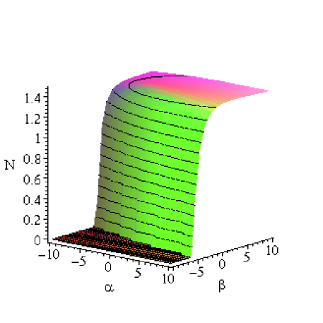
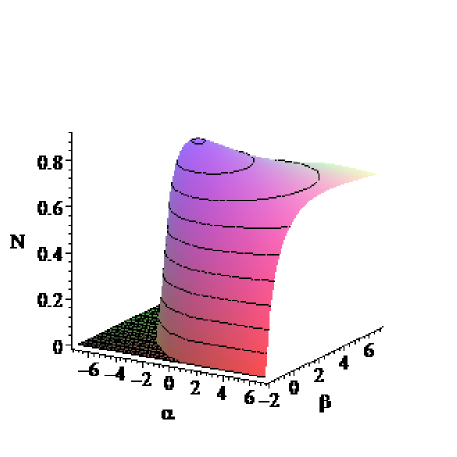
To the parameters given in (II.3) or (II.3), the number of e-folds is of order unity, see Figs. 1 and 2. However, this is not a disaster, since the universe would have been expanding prior to the period of transient acceleration, with the number of e–folds

$$\overline{N}_{e}=\int\frac{\dot{a}}{a}\,{{\rm d}t}=\int_{\tilde{u}}^{u_{-}}\frac{a^{\prime}}{a}{\rm d}u.$$ (36)

If $\Delta u=|u_{-}-\tilde{u}|\lesssim{10}^{-36}$, then it is not impossible that the total number of e-folds $\overline{N}_{e}+N_{e}>60$, as required to explain the flatness problem. In our model, it is possible that the scale factor of our universe remained much larger than the size of internal dimensions at the beginning of the accelerating epoch.

II.4 The field equations in $\delta=0$ gauge

Let us consider the case where, at least, one of the $\sigma_{i}$ is non-zero. We also demand that $f>0$. In this case we find it convenient to choose the gauge $\delta=0$ in the metric ansatz (2), so that $u$ becomes the (proper) cosmic time, $t$, and $\phi_{i}\equiv\phi_{i}(t)$. Then upon dimensional reduction from $(4+n)$ dimensions to four-dimensions, we get

$$I=\frac{1}{8\pi G_{4}}\int{d^{4}x}\sqrt{-g_{4}}\left(\frac{R_{4}}{2}+K-V\right),$$ (37)

where $G_{4}=G_{4+n}/\text{Vol}({\cal M}^{n})$. The kinetic term $K$ is given by (7), after replacing the time derivative ${}^{\prime}=\partial/\partial{u}$ by $\dot{}=\partial/\partial{t}$, along with the substitutions: $m_{1}=p$, $m_{2}=2q$ and $m_{3}=1$. While, the potential term is given by

$$V=\Lambda_{1}e^{-(p+2)\phi_{1}-2q\phi_{2}-\phi_{3}}+\Lambda_{2}e^{-p\phi_{1}-2(q+1)\phi_{2}-\phi_{3}}+q{F}^{2}e^{-p\phi_{1}-2(q+2)\phi_{2}+\phi_{3}}\equiv V_{1}+V_{2}+V_{F},$$ (38)

where $\Lambda_{1}=-\epsilon_{1}\frac{p(p-1)}{2r_{\lower 2.0pt\hbox{$\scriptstyle 1$}}^{2}}$, $\Lambda_{2}=-\epsilon_{2}\frac{q}{r_{\lower 2.0pt\hbox{$\scriptstyle 2$}}^{2}}$ and $F=(f/2)(r_{\lower 2.0pt\hbox{$\scriptstyle 3$}}/r_{\lower 2.0pt\hbox{$\scriptstyle 2$}}^{2})$. The analogue Einstein equations are

$\displaystyle\ddot{\Phi}+3\frac{\dot{a}}{a}\dot{\Phi}-2K-3\frac{\ddot{a}}{a}=0,$ (39)
$\displaystyle\ddot{\Phi}+3\frac{\dot{a}}{a}\dot{\Phi}-2\left(\frac{\dot{a}}{a}\right)^{2}-\frac{\ddot{a}}{a}-\frac{2k}{a^{2}}=0,$ (40)
$\displaystyle\ddot{\phi_{1}}+3\frac{\dot{a}}{a}\dot{\phi}_{1}-\frac{2}{p}V_{1}=0,$ (41)
$\displaystyle\ddot{\phi_{2}}+3\frac{\dot{a}}{a}\dot{\phi}_{2}-\frac{1}{q}V_{2}-\frac{2}{q}V_{F}=0,$ (42)
$\displaystyle\ddot{\phi_{3}}+3\frac{\dot{a}}{a}\dot{\phi}_{3}+2V_{F}=0,$ (43)

where $\Phi=p\phi_{1}/2+q\phi_{2}+\phi_{3}/2$. In terms of alternative canonically normalized scalars, which may be defined by

$\displaystyle\varphi_{1}=\sqrt{\frac{q}{2(q+1)}}\left(p\phi_{1}+2(q+1)\phi_{2}+\phi_{3}\right),$
$\displaystyle\varphi_{2}=\sqrt{\frac{p(p+2q+2)}{2(q+1)}}\left(\phi_{1}+\frac{1}{p+2q+2}\phi_{3}\right),$
$\displaystyle\varphi_{3}=-\sqrt{\frac{p+2q+3}{p+2q+2}}\phi_{3},$ (44)

the field equations take the following form

$$\ddot{\varphi_{i}}+3H\dot{\varphi_{i}}+\frac{dV}{d\varphi_{i}}=0,$$ (45)
$$\dot{H}+K-ka^{-2}=0,$$ (46)

along with the Friedmann (constraint) equation

$$H^{2}=\frac{1}{3}\left(K+V\right)-ka^{-2},$$ (47)

where $K=\frac{1}{2}\sum_{i}^{3}\dot{\varphi_{i}}^{2}$. The resulting scalar potential is

$$V=\Lambda_{1}{\rm e}^{-\beta_{1}\varphi_{1}-\beta_{2}\varphi_{2}}+\Lambda_{2}{\rm e}^{-2\varphi_{1}/\beta_{1}}+qF^{2}{\rm e}^{-\beta_{3}\varphi_{1}+\beta_{4}\varphi_{2}-\beta_{5}\varphi_{3}},$$ (48)

where

$\displaystyle\beta_{1}\equiv\sqrt{\frac{2q}{q+1}},\quad\beta_{2}\equiv\sqrt{\frac{2(p+2q+2)}{p(q+1)}},\quad\beta_{3}\equiv\frac{q+2}{q}\beta_{1},$
$\displaystyle\beta_{4}\equiv\frac{2}{q+1}\frac{1}{\beta_{2}},\quad\beta_{5}\equiv 2\sqrt{\frac{p+2q+3}{p+2q+2}}.$ (49)

Clearly the potential has a positive definite minimum with respect to a subset of the $\varphi_{i}$ directions. By comparing the $f=0$ and $f>0$ potentials, we see that a geometric twist has a more significant influence on shape of the potential. In general, a scalar potential as above, with cross coupling exponents, implies the existence of a local de Sitter region. Thus one may expect that accelerating cosmologies with a larger number of e-folds is possible in this case.

It is rather non-trivial to write the general solution of equations (45)-(47) with the potential (48), in terms of proper (cosmic) time $t$, but any such solutions should be the same as the one from $4+n$ dimensional field equations. Accepting that the effective potential is a useful tool in this investigation, in later Sections we present various explicit solutions that correspond to the above set of equations, but in terms of a new time coordinate, $\tau$.

II.5 M-theory phantom cosmology

Let us first briefly discuss a special case where the scalar potential $V(\varphi)=0$. With $\Lambda_{i}=0=F^{2}$, the solution for the scalars is

$$\dot{\phi_{i}}(t)=\sqrt{3}\frac{c_{i}\,a_{0}^{2}}{a(t)^{3}},$$ (50)

where a dot denotes differentiation with respect to cosmic time $t$. The factor of $\sqrt{3}$ is introduced just for a convenience. The corresponding kinetic term is

$$K=3C\frac{{a_{0}}^{4}}{a(t)^{6}},$$ (51)

where

$$C\equiv 6c_{1}^{2}+2c_{2}^{2}+\frac{3}{4}c_{3}^{2}+4c_{1}c_{2}+c_{2}c_{3}+2c_{1}c_{3}.$$ (52)

The effective potential, say $\tilde{V}$, can have a non-zero contribution if the intrinsic curvature of the physical 3-space is non-zero, $k\neq 0$, see e.g. CHNW03b . In the $k=-1$ case, the solution for the scale factor is implicitly given by

$$\int^{a(t)}\frac{x^{2}}{\sqrt{x^{4}+Ca_{0}^{4}}}dx=t+t_{1}.$$ (53)

where $t_{1}$ is an arbitrary constant. The $C=0$ solution is special, as it implies $a(t)=t+t_{2}$ and $\ddot{a}=0$. This solution critically differentiates between eternally accelerating expansion (if $C<0$) and decelerating expansion ($C>0$). In the case $K=V(\varphi)=0$, the cosmological trajectories can be the null geodesics in a Milne patch ($k=-1$) of 4d Minkowski spacetime, following Townsend:2004zp

The choice where all $c_{i}$ are zero except one corresponds to phantom cosmology, if the non-vanishing $c_{i}$ is imaginary. In this case, since $C<0$ (or $K<0$), the corresponding solution yields $\mbox{w}<-1$, where $\mbox{w}\equiv(K-\tilde{V})/(K+\tilde{V})$, and also that $\mbox{w}\to-1$ as $t\to\infty$ (for a discussion of phantom cosmology with a single scalar in exponential form, see, e.g. Refs. Sami:2003xv ; Nojiri0405 ). In our model, however, the choice $C<0$ is not physically motivated, because in this case some of the extra dimensions behave as time-like, rather than space-like.

III Multiple scalars and cosmology in four-dimensions

In this Section, we give a general discussion on solving scalar field equations with multiple exponential potentials in a flat FRW universe. First, we note that for the compactification of classical supergravities on product spaces, with or without certain ‘twists’ in the geometry twist, one can always bring the scalar potential into the form

$$V(\varphi)=\sum_{i=1}^{s}\Lambda_{i}\,{\rm e}^{-\frac{1}{M_{P}}\sum_{i\geq j\geq 1}^{i+j-1}\lambda_{i+j-1}\varphi_{j}},$$ (54)

where $\varphi_{i}$ are canonically normalized 4d scalars. The kinetic term is given by $K=\frac{1}{2}\sum_{i}^{s}\dot{\varphi}_{i}^{2}$. The corresponding equations of motion for the scalar fields are

$$\ddot{\varphi}_{i}+3H\dot{\varphi}_{i}+\frac{dV}{d\varphi_{i}}=0,$$ (55)

while the Friedmann equation is

$$H^{2}=\frac{\rho_{\varphi}}{3M_{P}^{2}}-\frac{k}{a^{2}},$$ (56)

where $a$ is the scale factor, $H\equiv\dot{a}/a$ is the Hubble parameter, which represents the universal rate of expansion, $\rho_{\varphi}\equiv K+V(\varphi)$ is the energy density of the scalar fields, $k$ is the spatial curvature.

The values of (dilaton) coupling constant $\lambda_{i}$ are model or compactification scheme dependent, e.g. in the case of two scalars arising from hyperbolic compactification of (4+m) dimensional supergravity CHNW03b , we find $\lambda_{1}={2}/{\lambda_{2}}=\pm\sqrt{2+4/m_{1}}$ and $\lambda_{3}=2\sqrt{(m_{1}+m_{2}+2)/[m_{2}(m_{1}+2)]}$. Further, $\Lambda_{i}=-\epsilon_{i}\frac{m_{i}(m_{i}-1)}{2}\,\left(\frac{M_{P}}{r_{i}}\right)^{2}$, so that $\epsilon_{i}=0,+1$ or $-1$, respectively, for flat, spherical or hyperbolic space.

III.1 The two scalar case

Consider the potential with $2$ scalars $\varphi_{1},\varphi_{2}$:

$\displaystyle V(\varphi)$ $\displaystyle=$ $\displaystyle{\Lambda_{1}}\,{\rm e}^{-{\lambda_{1}}\varphi_{1}}+{\Lambda_{2}}\,{\rm e}^{-{\lambda_{2}}\varphi_{1}-{\lambda_{3}}\varphi_{2}}$ (57)

(in units $M_{P}^{-1}=1$). The exact solution with the single scalar $\varphi_{1}$ has appeared in Townsend03b (Ref. IPN03d provides further generalizations, and Ref. Chimento98a ; jrusso04a contain solutions in different time coordinates). In the $\Lambda_{2}=0$ case, the field $\varphi_{2}$ acts merely as a non-interacting massless scalar. This case was studied in Chimento98a . Thus we focus here on solutions with more than one scalars, where in general $\Lambda_{i}\neq 0$. We present solutions with two and three scalars, but the method would be equally applicable to higher number of scalar fields.

In the two scalar case, the late time behavior of the scale factor and the scalars is characterized by

$$a(t)\propto\left\{\begin{array}[]{l}(t/t_{0})^{\gamma},~{}~{}~{}~{}~{}~{}~{}~{}\quad k=0,\\ \\ \sqrt{|k|}\,t,~{}~{}~{}~{}~{}~{}~{}~{}~{}\quad k\neq 0,\end{array}\right.$$ (58)
$$\varphi_{1}=\frac{1}{\lambda_{1}}\left(2\ln{t}-\ln\arrowvert{\varphi_{1}^{(0)}}\arrowvert\right),\quad\varphi_{2}=\frac{1}{\lambda_{1}}\left(2\mu\ln{t}+\frac{\lambda_{2}}{\lambda_{3}}\ln\arrowvert{\varphi_{1}^{(0)}}\arrowvert-\frac{\lambda_{1}}{\lambda_{3}}\ln\arrowvert{\varphi_{2}^{(0)}}\arrowvert\right),$$ (59)

where

$\displaystyle\gamma\equiv\frac{2(1+\mu^{2})}{\lambda_{1}^{2}},\quad\mu\equiv\frac{\lambda_{1}-\lambda_{2}}{\lambda_{3}},$ (60)
$\displaystyle\varphi_{1}^{(0)}=\frac{2(3p-1)}{\Lambda_{1}\lambda_{1}^{2}}\left(1-\frac{\lambda_{2}}{\lambda_{3}}\mu\right),\quad\varphi_{2}^{(0)}=\frac{(3p-1)}{\Lambda_{2}}\frac{2\mu}{\lambda_{1}\lambda_{3}}.$ (61)

The late time attractor solutions, with $\Lambda_{1}=0$, have appeared before in Ref. Ed99a . Since these asymptotic solutions may not be taken to far, below we present a more general class of solutions which are available before the attractors are reached.

III.2 Accelerating solutions

With any number of scalars, there would be a period of acceleration (where $\dot{a}>0,~{}\ddot{a}>0$) before approaching the attractor provided that $\gamma>1/3$. The universe inflates when one of the fields approaches its minimum, where the energy density is dominated by the potential energy of scalar fields. In particular, the solution around $\varphi_{1}=0$ and $\varphi_{2}=\frac{c_{\lower 2.0pt\hbox{$\scriptstyle 0$}}}{\lambda_{3}}$ ($c_{\lower 2.0pt\hbox{$\scriptstyle 0$}}$ is defined below) is given by

$$a(t)=\left\{\begin{array}[]{l}a_{0}\,{\rm e}^{H_{0}\,t},~{}~{}~{}~{}~{}~{}~{}~{}~{}~{}~{}~{}~{}~{}~{}~{}~{}~{}~{}\quad k=0,\\ \\ (\sqrt{k}/H_{0})\,\cosh{H_{0}\,t},~{}~{}~{}~{}~{}\quad k>0,\\ \\ (\sqrt{-k}/H_{0})\,\sinh{H_{0}\,t},~{}~{}~{}\quad k<0,\end{array}\right.$$ (62)

where the Hubble rate $H_{0}$ is characterized by the scale

$$H_{0}=\sqrt{\frac{\gamma^{2}}{\varphi_{1}^{(0)}}}.$$ (63)

In a flat universe the solution (62) is held only as an intermediate stage in the evolution unless $\gamma>1$. For $k\neq 0$, however, the period of acceleration depends on the initial value of $\varphi_{i}$, other than the couplings $\lambda_{i}$. The inflating $k=-1$ slice that approaches the geodesic $a(t)\sim{t}$ asymptotically can be eternally accelerating even if $\gamma<1$, as in the single scalar double exponential case Jarv04a ; IPN03d .

To find the exact solution, with $k=0$, one introduces a new logarithmic time variable $\tau$, which is defined by

$$\alpha=\ln(a(t)),\quad\tau=\int^{t}{\rm e}^{-\lambda_{1}\varphi_{1}(\bar{t})/2}{\rm d}\bar{t}.$$

For $k=0$, the field equations (55)-(56), with $i=1,2$, reduce to

$\displaystyle\alpha^{\prime}$ $\displaystyle=$ $\displaystyle\frac{1}{2\sqrt{3}}\sqrt{V_{0}}\left(\xi+\xi^{-1}\right),$ (64)
$\displaystyle\varphi_{1}^{\prime}$ $\displaystyle=$ $\displaystyle\frac{1}{\sqrt{2}}\sqrt{V_{0}}\sqrt{1+\mu^{2}}\left(\xi-\xi^{-1}\right),$ (65)
$\displaystyle\varphi_{2}$ $\displaystyle=$ $\displaystyle\mu\varphi_{1}+\lambda_{\lower 2.0pt\hbox{$\scriptstyle 3$}}^{-1}c_{\lower 2.0pt\hbox{$\scriptstyle 0$}},$ (66)

where a prime denotes differentiation w. r. to $\tau$,

$$V_{0}\equiv\Lambda_{\lower 2.0pt\hbox{$\scriptstyle 1$}}+\Lambda_{\lower 2.0pt\hbox{$\scriptstyle 2$}}{\rm e}^{-c_{\lower 2.0pt\hbox{$\scriptstyle 0$}}},\quad c_{\lower 2.0pt\hbox{$\scriptstyle 0$}}\equiv\ln|\frac{\Lambda_{\lower 2.0pt\hbox{$\scriptstyle 2$}}}{\Lambda_{\lower 2.0pt\hbox{$\scriptstyle 1$}}}\,\frac{\lambda_{3}^{2}-\lambda_{2}(\lambda_{1}-\lambda_{2})}{\lambda_{1}(\lambda_{1}-\lambda_{2})}|$$ (67)

and the variable $\xi$ satisfies the differential equation

$$\xi^{\prime}=\sqrt{V_{\lower 2.0pt\hbox{$\scriptstyle 0$}}}(4\gamma)^{-1/2}\left((\sqrt{3\gamma}+1)-(\sqrt{3\gamma}-1)\xi^{2}\right).$$ (68)

The $k=0$ hyperbola $3{\alpha^{\prime}}^{2}-(1+\mu^{2}){\varphi_{1}^{\prime}}^{2}/2=V_{0}$ separates the $k=+1$ and $k=-1$ trajectories. Though it is rather non-trivial to write the solutions explicitly when $k=\pm 1$, one may extract the common physical effects by studying the trajectories in a phase portrait, following Jarv04a ; halliwell .

Let us consider the $\alpha^{\prime}>0$ branch, which restricts the solution to expanding cosmologies. For $\gamma>1/3$, the explicit solution is

$$\xi=\sqrt{\frac{\sqrt{3\gamma}+1}{\sqrt{3\gamma}-1}}\tanh\sqrt{V_{0}}\sqrt{\frac{3\gamma-1}{4\gamma}}\tau,$$ (69)

up to a shift of $\tau$ about $\tau=0$. Hence

$\displaystyle a$ $\displaystyle=$ $\displaystyle a_{0}\left(\cosh\zeta\tau\right)^{\delta_{-}}\left(\sinh\zeta\tau\right)^{\delta_{+}},$ (70)
$\displaystyle\varphi_{1}$ $\displaystyle=$ $\displaystyle\frac{1}{\beta}\ln\left(\left(\cosh\zeta\tau\right)^{\delta_{-}}\left(\sinh\zeta\tau\right)^{-\delta_{+}}\right)+\varphi_{0},$ (71)

where $\beta\equiv\sqrt{(1+\mu^{2})/6}$,

$$\delta_{\pm}=\sqrt{\frac{\gamma}{3}}\frac{1}{\sqrt{3\gamma}\pm 1},\quad\zeta=\sqrt{V_{0}}\sqrt{\frac{3\gamma-1}{4\gamma}}$$ (72)

and $a_{0}$ and $\varphi_{0}$ are integration constants. To obtain the solution for $\gamma<1/3$, one replaces $\tanh{X}$ by $\tan{X}$ in (69). Since the scaling regime of exponential potentials does not depend upon its compactification or mass scales ($\Lambda_{i}$), $\varphi_{0}$ is actually a free parameter that can, for simplicity, be set to $M_{P}$ or even to zero.

The acceleration parameter is given by

$$\frac{\ddot{a}}{a}={2\zeta^{2}}\,{\rm e}^{-\sqrt{\frac{12}{\gamma}}\beta\varphi_{1}}\left[4\delta_{-}\delta_{+}-(\delta_{-}\tanh\zeta\tau)^{2}-(\delta_{+}\coth\zeta\tau)^{2}\right],$$ (73)

which decreases as $\tau$ increases. This actually implies that the $\tau\to\infty$ limit corresponds to $t\to\infty$, to the above solutions. It follows from (73) that, when $\gamma<1$, the solution will exhibit a period of transient acceleration. This occurs on the interval $\tau_{-}<\tau<\tau_{+}$, where

$$(\tanh\zeta\tau_{\pm})^{2}=\frac{(2\pm\sqrt{3})(\sqrt{3\gamma}-1)}{\sqrt{3\gamma}+1}.$$ (74)

For future use, we also note that the shift in $\varphi_{1}$ during the accelerated epoch is given by

$$\delta\varphi_{1}=\frac{1}{\beta}\left[\delta_{-}\ln\frac{\cosh\zeta\tau_{+}}{\cosh\zeta\tau_{-}}-\delta_{+}\ln\frac{\sinh\zeta\tau_{+}}{\sinh\zeta\tau_{-}}\right],$$ (75)

while $\delta\varphi_{2}=\mu\delta\varphi_{1}$. At late times, $\tau\to\infty$ (or $t\to\infty$), we find

$$\frac{\ddot{a}}{a}\propto\frac{\gamma(\gamma-1)}{(3\gamma-1)^{2}}.$$ (76)

An important difference between $\gamma>1$ and $\gamma=1$ solutions is that in the formal case the number of e-folds is arbitrary, while in the latter it is fixed, $N_{e}=11.68$. Thus, the $\gamma=1$ solution may be viewed as a transient only since it has got a natural entry and exit from inflation; the period of acceleration can be made arbitrary large but not the e-folds!

The number of e-folds $N_{e}$ during the accelerated epoch is given by

$$N_{e}=\int_{t_{i}}^{t_{f}}H{\rm d}t=\int_{\tau_{-}}^{\tau_{+}}\frac{a^{\prime}}{a}{\rm d}\tau=\int_{\tau_{-}}^{\tau_{+}}\zeta\left(\delta_{-}\tanh\zeta\tau+\delta_{+}\coth\zeta\tau\right),$$ (77)

where $t_{i}$ and $t_{f}$ are the starting and ending times of the accelerated expansion. The parameters $\delta_{\pm}$ and $\zeta$ are constants which were defined previously in (72).

For $\gamma<1$, the number of e-folds during an acceleration epoch is given analytically by

$$N_{e}=\frac{\gamma}{3\gamma-1}\ln\frac{(3-\sqrt{3})(1+\sqrt{\gamma})}{(3+\sqrt{3})(1-\sqrt{\gamma})}+\sqrt{\frac{\gamma}{3}}\frac{1}{\sqrt{3\gamma}-1}\ln\frac{\sqrt{3}+1}{\sqrt{3}-1}.$$ (78)

As some specific values, one has $N_{e}=2.62$ for $\gamma=0.99$; $N_{e}=1.5$ for $\gamma=0.9$; $N_{e}=1.16$ for $\gamma=0.8$. It is worth noting that the number of e-folds depends only upon the effective value of the acceleration parameter $\gamma$, but not on the number of scalar fields.

In the $\gamma\leq 1$ case, both the lower and the upper limits ($\tau_{-}$ and $\tau_{+}$) are fixed in terms of $\zeta$ and $\gamma$, while, in the $\gamma>1$ case, only the lower limit of integration (the on-set time of accelerated epoch) is fixed, which is given by

$$\tau_{-}=\frac{1}{\zeta}\tanh^{-1}\sqrt{\frac{(2-\sqrt{3})(\sqrt{3\gamma}-1)}{\sqrt{3\gamma}+1}}.$$ (79)

III.3 The three scalar case

It is straightforward to generalize the above results with higher number of scalar fields. Let us consider the potential with $3$ scalars $\varphi_{1},\varphi_{2},\varphi_{3}$, which is given by

$$V={\Lambda_{1}}\,{\rm e}^{-\lambda_{1}\varphi_{1}}+{\Lambda_{2}}{\rm e}^{-\lambda_{2}\varphi_{1}-\lambda_{3}\,\varphi_{2}}+{\Lambda_{3}}\,{\rm e}^{-\lambda_{4}\varphi_{1}-\lambda_{5}\varphi_{2}-\lambda_{6}\varphi_{3}}.$$ (80)

The solution to the equations (55) (56), with the potential (80), is given by (70)-(71) but now

$$\beta\equiv\frac{1}{\sqrt{6}}\sqrt{1+\mu^{2}+\nu^{2}},\quad V_{\lower 2.0pt\hbox{$\scriptstyle 0$}}\equiv\Lambda_{1}+\Lambda_{2}{\rm e}^{-c_{\lower 2.0pt\hbox{$\scriptstyle 0$}}}+\Lambda_{3}{\rm e}^{-d_{\lower 2.0pt\hbox{$\scriptstyle 0$}}},$$ (81)

where

$\displaystyle\nu\equiv\frac{\lambda_{3}(\lambda_{1}-\lambda_{4})-\lambda_{5}(\lambda_{1}-\lambda_{2})}{\lambda_{3}\lambda_{6}},\quad\gamma=\frac{2}{\lambda_{1}^{2}}\left(1+\mu^{2}+\nu^{2}\right),$
$\displaystyle c_{\lower 2.0pt\hbox{$\scriptstyle 0$}}\equiv d_{\lower 2.0pt\hbox{$\scriptstyle 0$}}-\ln\left|\frac{\Lambda_{3}}{\Lambda 2}\,\frac{\mu\lambda_{6}-\nu\lambda_{5}}{\nu\lambda_{3}}\right|,$
$\displaystyle d_{\lower 2.0pt\hbox{$\scriptstyle 0$}}\equiv\ln\left|\frac{\Lambda_{3}}{\Lambda_{1}}\frac{\lambda_{6}(\lambda_{3}-\mu\lambda_{2})+\nu(\lambda_{2}\lambda_{5}-\lambda_{3}\lambda_{4})}{\lambda_{1}\lambda_{3}}\right|,$ (82)

and

$$\varphi_{2}=\mu\varphi_{1}+\lambda_{3}^{-1}c_{\lower 2.0pt\hbox{$\scriptstyle 0$}},\quad\varphi_{3}=\nu\varphi_{1}+\lambda_{6}^{-1}d_{\lower 2.0pt\hbox{$\scriptstyle 0$}}.$$ (83)

As for the attractor solutions, one reads $\varphi_{1},~{}\varphi_{2}$ from (59), while $\varphi_{3}$ is given by

$$\varphi_{3}=\frac{2\nu}{\lambda_{1}}\ln{t}-\frac{1}{\lambda_{6}}\ln\arrowvert{\varphi_{3}^{(0)}}\arrowvert+\frac{\lambda_{5}}{\lambda_{3}\lambda_{6}}\ln\arrowvert{\varphi_{2}^{(0)}}\arrowvert+\frac{\lambda_{3}\lambda_{4}-\lambda_{2}\lambda_{5}}{\lambda_{1}\lambda_{3}\lambda_{6}}\ln\arrowvert{\varphi_{1}^{(0)}}\arrowvert.$$ (84)

The constants $\varphi_{i}^{(0)}$ are now given by

$\displaystyle\frac{\Lambda_{1}\varphi_{1}^{(0)}}{3\gamma-1}$ $\displaystyle=$ $\displaystyle\frac{2}{\lambda_{1}^{2}}\left(1-\frac{\lambda_{2}(\lambda_{5}^{2}+\lambda_{6}^{2})-\lambda_{1}\lambda_{3}\lambda_{5}}{\lambda_{3}\lambda_{6}^{2}}\mu-\frac{\lambda_{4}\nu}{\lambda_{3}\lambda_{6}}\right),$
$\displaystyle\frac{\Lambda_{2}\varphi_{2}^{(0)}}{3\gamma-1}$ $\displaystyle=$ $\displaystyle\frac{2}{\lambda_{1}\lambda_{3}}\left(\mu-\frac{\lambda_{5}\nu}{\lambda_{6}}\right),\quad\frac{\Lambda_{3}\varphi_{3}^{(0)}}{(3\gamma-1)}=\frac{2\nu}{\lambda_{1}\lambda_{6}}.$ (85)

Notice that only the product $\Lambda_{i}\varphi_{i}^{(0)}$ is fixed but not each term separately, so the increase of $\varphi_{1}^{(0)}$ to $\tilde{\varphi}_{1}^{(0)}$ can be absorbed by rescaling $\Lambda_{1}\to\Lambda_{1}\,(\tilde{\varphi}_{1}^{(0)}/\varphi_{1}^{(0)})$. The scalar fields $\varphi_{i}$ transform under scale transformations in a canonical way, i.e. $\varphi_{i}\to\varphi_{i}/L$.

IV de Sitter vacuum and cosmic acceleration

IV.1 Exponential potentials with more than one scalar

Let us first discuss some general features of the cosmological potential (48) with $F^{2}=0$. The corresponding solution will then exhibit a period of transient acceleration, with the number of e-folds

$$N_{e}=\frac{n-1}{2(n-2)}\ln\frac{3-\sqrt{3}}{3+\sqrt{3}}\frac{\sqrt{n+1}+\sqrt{n-1}}{\sqrt{n+1}-\sqrt{n-1}}+\sqrt{\frac{n-1}{3}}\frac{1}{\sqrt{3(n-1)}-\sqrt{n+1}}\ln\frac{\sqrt{3}+1}{\sqrt{3}-1},$$ (86)

where $n\equiv p+2q+1$. Thus the number of e-folds increases only marginally when the dimensions of the internal space are increased. The late time behavior of the scale factor is characterized by $a\propto t^{\gamma}$, where $\gamma=(n+1)/(n-1)$.

Let us consider some special cases, where one of the scalars $\varphi_{i}$ takes a (nearly) constant value. In this rather restricted case there can exist solutions with a large number of e-folds. One such example is to consider the potential (48), with $\Lambda_{2}=0,\,p=4,\,q=1$ and $\varphi_{1}=b_{1}=$const. Of course this will constrain the evolution of volume moduli and hence the 4d effective potential. In this case, the scalar potential is given by

$$V={\rm e}^{-b_{1}}\left(\Lambda_{1}{\rm e}^{-\sqrt{2}\varphi_{2}}+F^{2}{\rm e}^{-2b_{1}}{\rm e}^{\varphi_{2}/\sqrt{2}-3\varphi_{3}/\sqrt{2}}\right).$$ (87)

The explicit exact solution can be found in terms of a new logarithmic time variable $\tau$, defined by $\tau=\int^{t}{\rm d}\bar{t}\,\exp\left[-\varphi_{2}(\bar{t})/\sqrt{2}\right]$. The explicit solution is

$\displaystyle a=a_{0}\left(\cosh\zeta\tau\right)^{\delta_{-}}\left(\sinh\zeta\tau\right)^{\delta_{+}},\quad b_{\lower 2.0pt\hbox{$\scriptstyle 1$}}=\ln\frac{3\Lambda_{1}}{2V_{0}},$
$\displaystyle\varphi_{2}=\sqrt{\frac{18}{5}}\ln\left(\left(\cosh\zeta\tau\right)^{\delta_{-}}\left(\sinh\zeta\tau\right)^{-\delta_{+}}\right),\quad\varphi_{3}=\varphi_{2}+\frac{\sqrt{2}}{3}\ln\left(\frac{8}{9}\frac{F^{2}V_{0}^{2}}{\Lambda_{1}^{3}}\right),$ (88)

where

$$\delta_{\pm}=\frac{\sqrt{6}}{3(\sqrt{6}\pm 1)},\quad\zeta=\sqrt{\frac{5V_{0}}{8}},$$ (89)

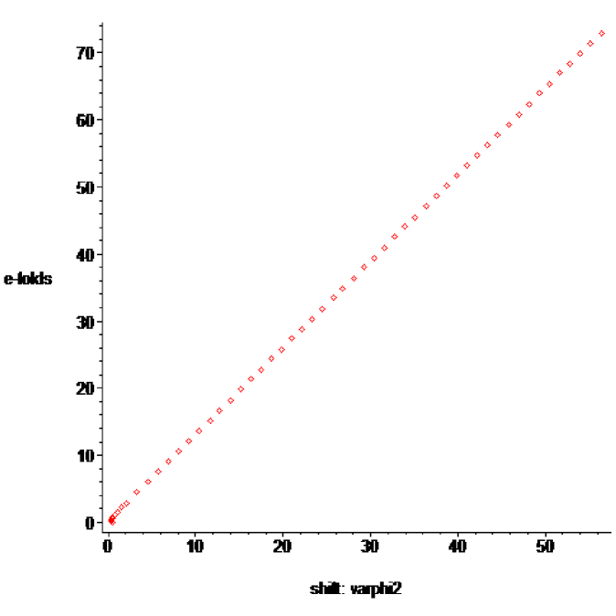
The total number of e-folds is given by

$\displaystyle N_{e}$ $\displaystyle=$ $\displaystyle\int H{\rm d}t$ (90)
$\displaystyle=$ $\displaystyle\int_{\tau_{0}}^{\tau_{-}}\frac{a^{\prime}}{a}{\rm d}\tau+\int_{\tau_{-}}^{\tau_{+}}\frac{a^{\prime}}{a}{\rm d}\tau.$

The contribution of the first integral will be known once $\tau_{0}$ is chosen, while that of the second term depends on $\tau_{+}$. As some representative values, with $V_{0}=1$, we find

$$N_{e}=55,~{}60,~{}65,\cdots,$$

respectively, when $\delta\varphi_{2}=41.91,\,45.78,\,49.65\cdots$ (see Fig. (3)). This gives only the minimum number of e-folds, since there is an extra contribution from the first integral in (90) (i.e. prior to the accelerated epoch), which we have dropped here.

Refer to caption

Figure 3: The number of e–folds $N$ vs scalar field $\varphi_{2}$, for the potential (87).

Let us consider some other possibilities, by allowing certain fine tunings among the scalars $\varphi_{i}$ or the volume moduli $\phi_{i}$. For the potential (48), the late time behavior of the scale factor may be characterized by $a(t)\propto t^{\gamma}$, where

$$\gamma=\left\{\begin{array}[]{l}\frac{q+1}{q}+\frac{2(p+2q+2)}{q^{2}(p+2q+3)}\qquad(\varphi_{2}=\text{const},\;\Lambda_{2}=0,\;\Lambda_{1}\neq 0,\;F^{2}\neq 0)\\ \frac{p(q+3)+q+1}{p+2q+3}\qquad\qquad(\varphi_{1}=\text{const},\;\Lambda_{2}=0,\;\Lambda_{1}\neq 0,\;F^{2}\neq 0)\\ \frac{q}{q+1}+\frac{p+2q+2}{2(q+1)^{2}(p+2q+3)}\qquad(\varphi_{2}=\text{const},\;\Lambda_{1}=0,\;\Lambda_{2}\neq 0,\;F^{2}\neq 0).\end{array}\right.$$ (91)

For instance, if $p=q=2$, the values of the expansion parameter $\gamma$, in the above three cases, are $35/18$, $13/9$ and $58/81$, respectively. In the first two cases, the amount of inflation (or the number of e-folds) can be (arbitrarily) large while it is small in the last case. In our model, when all scalar fields $\varphi_{i}$ vary with time, then a positive potential minimum representing the de Sitter phase of our universe can only be metastable. The different choice in the potentials could lead to the different asymptotic expansion of our universe.

IV.2 A model of eternal acceleration

Let us extend the above discussion by specializing the case with $p=4$ and $q=1$, but now we take the 4-space ${\cal M}^{4}$ as a direct product between two ${\cal M}^{2}$,s of arbitrary curvatures. The corresponding 11d metric Ansatz is

$${\rm d}s_{11}^{2}={\rm e}^{-2\Phi}{\rm d}s_{4}^{2}+r_{1}^{2}{\rm e}^{2\phi_{1}}{\rm d}s^{2}({\cal M}^{2}_{\epsilon_{1}})+r_{2}^{2}{\rm e}^{2\phi_{2}}{\rm d}s^{2}({\cal M}^{2}_{\epsilon_{2}})+r_{3}^{2}{\rm e}^{2\phi_{3}}({dx}^{2}+{dy}^{2})+r_{4}^{2}{\rm e}^{2\phi_{4}}\left(dz+\frac{f}{2}(x{dy}-y{dx})\right)^{2},$$ (92)

where $\Phi=\phi_{1}+\phi_{2}+\phi_{3}+\phi_{4}/2$, and ${\rm d}s_{4}^{2}$ is the standard FRW metric in the form (2). Here we work in units where the curvature radii $r_{i}$ are set to unity, as these variables may often be absorbed in $\epsilon_{i}$ (i.e. $\epsilon_{i}\to\epsilon_{i}/r_{i}^{2}$, where $\epsilon_{i}=0,\pm 1$) and/or in the twist parameter $f$. In the gauge $\delta=0$, upon reductions to four dimensions, the kinetic and potential terms are given by

$\displaystyle K$ $\displaystyle=$ $\displaystyle 2{\dot{\phi}_{1}}^{2}+2{\dot{\phi}_{2}}^{2}+2{\dot{\phi}_{3}}^{2}+3{\dot{\phi}_{1}}^{2}/4+2\dot{\phi}_{1}\dot{\phi}_{2}+2\dot{\phi}_{2}\dot{\phi}_{3}+2\dot{\phi}_{3}\dot{\phi}_{1}+\dot{\phi}_{1}\dot{\phi}_{4}+\dot{\phi}_{2}\dot{\phi}_{4}+\dot{\phi}_{3}\dot{\phi}_{4},$
$\displaystyle V$ $\displaystyle=$ $\displaystyle-\epsilon_{1}e^{-4\phi_{1}-2\phi_{2}-2\phi_{3}-\phi_{4}}-\epsilon_{2}e^{-2\phi_{1}-4\phi_{2}-2\phi_{3}-\phi_{4}}+\frac{f^{2}}{4}e^{-2\phi_{1}-2\phi_{2}-6\phi_{3}+\phi_{4}}.$ (93)

In terms of alternative canonically normalized scalars, which may be defined by

$\displaystyle\varphi_{1}=\phi_{1}+\phi_{2}+2\phi_{3}+\phi_{4}/2,\quad\varphi_{2}=\sqrt{3}\left(\phi_{1}+\frac{1}{3}\phi_{2}+\frac{1}{6}\phi_{4}\right),$
$\displaystyle\varphi_{3}=\sqrt{\frac{8}{3}}\left(\phi_{2}+\frac{1}{8}\phi_{4}\right),\quad\varphi_{4}=-\sqrt{\frac{9}{8}}\phi_{4},$ (94)

the corresponding field equations reduce to Eqs (55), (56) with $K=(1/2)\sum_{i}^{4}\dot{\varphi_{i}}^{2}$. The resulting scalar potential is

$$V=-\epsilon_{1}{\rm e}^{-\varphi_{1}-\sqrt{3}\varphi_{2}}-\epsilon_{2}{\rm e}^{-\varphi_{1}-\sqrt{\frac{1}{3}}\varphi_{2}-\sqrt{\frac{8}{3}}\varphi_{3}}+\frac{f^{2}}{4}{\rm e}^{-3\varphi_{1}+\sqrt{\frac{1}{3}}\varphi_{2}+\sqrt{\frac{1}{6}}\varphi_{3}-\sqrt{\frac{9}{2}}\varphi_{4}}.$$ (95)

For the potential (95), there is a local de Sitter minimum along $\varphi_{2}$, which is given by

$$\varphi_{2}^{(0)}=-\sqrt{3}\varphi_{1}-2\sqrt{2}\varphi_{3}-\frac{\sqrt{3}}{2}\ln\frac{\pm\sqrt{A^{2}-3B}-A}{6},$$ (96)

where

$$A\equiv\frac{\epsilon_{2}}{\epsilon_{1}}{\rm e}^{-2\varphi_{1}-2\sqrt{6}\varphi_{3}},\quad B\equiv\frac{{f}^{2}}{\epsilon_{1}}{\rm e}^{-6\varphi_{1}-\frac{5\sqrt{6}}{2}\varphi_{3}-\frac{3}{\sqrt{2}}\varphi_{4}}.$$

Of course, we are allowing here for the possibility that $A<0$, $B>0$ (i.e. $\epsilon_{1}=+1,\epsilon_{2}=-1$), in which case there can arise two local minima along $\varphi_{2}$. With $A<0$ (or $A>0$) and $B<0$, there is only one local (de Sitter) minimum. The solution with $A>0$, $B>0$ (i.e. $\epsilon_{1}=\epsilon_{2}=+1$) is, however, unstable.

Let us consider a special case where $\varphi_{1}=\mbox{const}\equiv b_{\lower 2.0pt\hbox{$\scriptstyle 0$}}$. An explicit exact solution can be found in terms of a logarithmic time variable $\tau$, defined by $\tau=\int^{t}{\rm d}\bar{t}\exp[-\sqrt{\frac{3}{4}}\,\varphi_{2}(\bar{t})]$. The solution is

$\displaystyle a=a_{\lower 2.0pt\hbox{$\scriptstyle 0$}}\left(\cosh\zeta\tau\right)^{\delta_{-}}\left(\sinh\zeta\tau\right)^{\delta_{-}},\quad\varphi_{1}=b_{\lower 2.0pt\hbox{$\scriptstyle 0$}},\quad\varphi_{2}=\sqrt{2}\ln\left[(\cosh\zeta\tau)^{\delta_{-}}(\sinh\zeta\tau)^{-\delta_{+}}\right],$
$\displaystyle\varphi_{3}=\frac{\varphi_{2}}{\sqrt{2}}+\sqrt{\frac{3}{32}}\ln\left(\frac{3\epsilon_{2}^{2}}{2\epsilon_{1}^{2}}\right),\quad\varphi_{4}=\sqrt{\frac{3}{2}}\varphi_{2}+\frac{1}{3\sqrt{2}}\left(\ln\frac{3f^{4}}{32\epsilon_{1}^{2}}-4b_{\lower 2.0pt\hbox{$\scriptstyle 0$}}\right),$ (97)

where

$$\delta_{\pm}=\frac{\sqrt{6}}{3(\sqrt{6}\pm 1)},\quad\zeta=\sqrt{\frac{-5\,\epsilon_{1}}{8}}\sqrt{1+\sqrt{\frac{8}{3}}}\,{\rm e}^{-b_{\lower 2.0pt\hbox{$\scriptstyle 0$}}/2}.$$ (98)

The late time behavior of the solution is characterized by

$\displaystyle a(t)\propto t^{2},\quad\varphi_{1}=b_{0},\quad\varphi_{2}=\sqrt{\frac{4}{3}}\ln{t}+\mbox{const},$
$\displaystyle\varphi_{3}=\sqrt{\frac{2}{3}}\ln{t}+\mbox{const},\quad\varphi_{4}=\sqrt{2}\ln{t}+\mbox{const}.$ (99)

In terms of the original volume scalars $\phi_{i}$, we find

$${\rm e}^{\phi_{1}},{\rm e}^{\phi_{2}}\propto t^{2/3},\quad{\rm e}^{\phi_{3}}\propto t^{-1/3},\quad{\rm e}^{\phi_{4}}\propto t^{-4/3}.$$ (100)

In this example the space $(T^{2}\ltimes S^{1})$ shrinks with time, though with different time-varying factors, while the 4-space ${\cal M}^{4}$ expands.

V More than one geometric twist

V.1 string/M theory with double twist

Consider an 11d metric ansatz such that

$$\Sigma_{7}=({\cal M}^{2}_{\epsilon_{1}}\ltimes S^{1})\times({\cal M}^{2}_{\epsilon_{2}}\ltimes S^{1})\times S^{1}.$$ (101)

We assign to each factor spaces the different time-varying scales: $e^{\phi_{1}},e^{\phi_{2}},\cdots,e^{\phi_{5}}$, where, in general, $\phi_{1}\neq\phi_{2}$, $\phi_{3}\neq\phi_{4}$. We also introduce the two non-trivial twist parameters, $f_{1}$ and $f_{2}$, and choose the Einstein conformal frame by setting $\Phi=\phi_{1}+\phi_{2}/2+\phi_{3}+\phi_{4}/2+\phi_{5}/2$.

We will begin by presenting a special exact solution where $\epsilon_{i}=0$ (so ${\cal M}^{2}\to\mathbb{T}^{2}$) and each 2-space $\mathbb{T}^{2}$ has the same time-varying volume. In this case, in the gauge $\delta=3$, the solution will be qualitatively similar to that with a single twist, namely,

$\displaystyle a=a_{0}\cosh(\chi{u})\,{\rm e}^{-\frac{1}{2}(8c+c_{2})u},$ (102)
$\displaystyle\phi_{1}=\ln\cosh\chi{u}-\frac{1}{2}(6c+c_{2})u=\phi_{3},$
$\displaystyle\phi_{2}=-\phi_{1}+c_{1}u+\ln\frac{f_{2}}{f_{1}}+\phi_{0}=\phi_{4}+\ln\frac{f_{2}}{f_{1}},$
$\displaystyle\phi_{5}=c_{2}u,\quad f_{1}f_{2}=2\chi^{2}/a_{0}^{6},$

where

$$\chi=\frac{1}{2}\sqrt{48c^{2}+12cc_{2}-8c_{1}^{2}-2c_{2}^{2}-4c_{1}c_{2}}.$$ (103)

This solution will of course exhibit only a period of transient acceleration, with number of e-folds ${N}_{e}={\cal O}(1)$. However, there can arise new solutions with a larger number of e-folds, especially, with a non-zero curvature, $\epsilon_{i}\neq 0$.

Let us consider another canonical example, but with six extra dimensions, i.e. $\Sigma_{6}=(\mathbb{T}^{2}\ltimes S^{1})\times(\mathbb{T}^{2}\ltimes S^{1})$. In this case, the explicit solution may be given by

$\displaystyle a(u)=a_{\lower 2.0pt\hbox{$\scriptstyle 0$}}\cosh(2c{u})\,{\rm e}^{{4}cu/\sqrt{3}},$
$\displaystyle\phi_{1}=\phi_{3}=\sqrt{3}c{u}+\ln\cosh(2c{u}),$
$\displaystyle\phi_{2}=-\phi_{1}+\ln\arrowvert\frac{f_{2}}{f_{1}}\arrowvert+\phi_{0}=\phi_{4}+\ln\arrowvert\frac{f_{2}}{f_{1}}\arrowvert,$ (104)

subject to the constraint

$$\quad f_{1}f_{2}=\frac{8c^{2}}{a_{\lower 2.0pt\hbox{$\scriptstyle 0$}}^{6}},$$ (105)

where $a_{\lower 2.0pt\hbox{$\scriptstyle 0$}}$, $c$ and $\phi_{\lower 2.0pt\hbox{$\scriptstyle 0$}}$ are integration constants. This solution can be obtained also from (102) after the substitutions: $c\to-c/\sqrt{3}$, $c_{1}=0$ and also $c_{2}=0$, as there is no $\phi_{5}$.

V.2 Some special solutions

Let us consider that the internal 7-space is split as in (101). But now we take $\epsilon_{i}\neq 0$. Upon reductions to four dimensions, we find that the scalar potential due to the non-trivial geometric twists, $f_{i}>0$, is given by

$$V(f_{i},\varphi_{i})=\frac{f_{2}^{2}}{4}e^{-\sqrt{\frac{2}{3}}\varphi_{1}-\sqrt{\frac{1}{3}}\varphi_{2}-\sqrt{\frac{25}{3}}\varphi_{3}+\sqrt{\frac{1}{6}}\varphi_{4}-\sqrt{\frac{9}{2}}\varphi_{5}}+\frac{f_{1}^{2}}{4}\,e^{\sqrt{\frac{2}{3}}\varphi_{1}-\sqrt{\frac{4}{3}}\varphi_{2}-\sqrt{\frac{4}{3}}\varphi_{3}-\sqrt{\frac{32}{3}}\varphi_{4}},$$ (106)

while, the curvature contribution to a scalar potential is given by

$$V(\epsilon_{i},\varphi_{i})=-{\epsilon_{1}}\,e^{-\sqrt{\frac{2}{3}}\varphi_{1}-\sqrt{\frac{1}{3}}\varphi_{2}-\sqrt{\frac{1}{3}}\varphi_{3}-\sqrt{\frac{8}{3}}\varphi_{4}}-{\epsilon_{2}}\,e^{-\sqrt{\frac{2}{3}}\varphi_{1}-\sqrt{\frac{1}{3}}\varphi_{2}-\sqrt{3}\varphi_{3}},$$ (107)

where $\varphi_{i}$ are canonically normalized four-dimensional scalars, defined in the following combinations:

$\displaystyle\varphi_{1}=\sqrt{\frac{1}{6}}(2\phi_{1}+3\phi_{2}+2\phi_{3}+\phi_{4}+\phi_{5}),\quad\varphi_{2}=\sqrt{\frac{1}{12}}(2\phi_{1}+2\phi_{3}+4\phi_{4}+\phi_{5}),$
$\displaystyle\varphi_{3}=\sqrt{\frac{1}{3}}(\phi_{1}+3\phi_{3}+\phi_{5}/2),\quad\varphi_{4}=\sqrt{\frac{1}{24}}(8\phi_{1}+\phi_{5}),\quad\varphi_{5}=-\sqrt{\frac{9}{8}}\phi_{5}.$ (108)

The total scalar potential is then given by $V=V(f_{i},\varphi_{i})+V(\epsilon_{i},\varphi_{i})$.

One may find various exact solutions by specializing the potential $V$ to some particular models, such as

$\displaystyle\varphi_{1},\,\varphi_{2}=\mbox{const}\Rightarrow\phi_{2}=\phi_{4}+\mbox{const},$
$\displaystyle\varphi_{2},\,\varphi_{3}=\mbox{const}\Rightarrow\phi_{3}=\phi_{4}+\mbox{const},$
$\displaystyle\varphi_{1},\,\varphi_{3}=\mbox{const}\Rightarrow 3\phi_{2}+\phi_{4}-4\phi_{3}=\mbox{const}.$

Let us consider the first case, where each 2-space ${\cal M}^{2}$ will have the same time-varying volume, by further setting $f_{1}=0$, $\epsilon_{1}=+1$ and $\epsilon_{2}=-1$, but $f_{\lower 2.0pt\hbox{$\scriptstyle 2$}}>0$. In terms of a logarithmic time variable $\tau=\int^{t}{\rm d}\bar{t}\exp[-\sqrt{3}\,\varphi_{3}(\bar{t})/2]$ or ${\rm d}\tau={\rm e}^{-\sqrt{3}\varphi_{3}/2}{\rm d}t$, the explicit solution is found to be

$\displaystyle a=a_{\lower 2.0pt\hbox{$\scriptstyle 0$}}\left(\cosh\zeta\tau\right)^{\delta_{-}}\left(\sinh\zeta\tau\right)^{\delta_{-}},$
$\displaystyle\varphi_{1}=b_{\lower 2.0pt\hbox{$\scriptstyle 1$}}=\mbox{const},\quad\varphi_{2}=b_{\lower 2.0pt\hbox{$\scriptstyle 2$}}=\mbox{const},$
$\displaystyle\varphi_{3}=\sqrt{\frac{18}{5}}\ln\left[(\cosh\zeta\tau)^{\delta_{-}}(\sinh\zeta\tau)^{-\delta_{+}}\right]+\varphi_{0},$
$\displaystyle\varphi_{4}=\frac{\varphi_{3}}{\sqrt{2}}-\frac{\sqrt{3}}{4\sqrt{2}}\left(\ln{3}-\ln{2}\right),$
$\displaystyle\varphi_{5}=-\frac{\varphi_{3}}{\sqrt{6}}-\frac{1}{3\sqrt{2}}\left(\ln{3}+\ln{2}-4\ln{f_{2}}\right),$

where

$$\delta_{\pm}=\frac{\sqrt{10}}{3(\sqrt{10}\pm\sqrt{3})},\quad\zeta=\sqrt{\frac{21(4-\sqrt{6})}{160}}{\rm e}^{-(\sqrt{2}b_{1}+b_{2})/\sqrt{12}}.$$ (110)

The late time behavior of the solution may be characterized by

$\displaystyle a(t)\propto t^{10/9},\quad\varphi_{3}=\sqrt{\frac{4}{3}}\ln{t}+\mbox{const},$
$\displaystyle\varphi_{4}=\sqrt{\frac{2}{3}}\ln{t}+\mbox{const},\quad\varphi_{5}=\sqrt{\frac{2}{9}}\ln{t}+\mbox{const}.$ (111)

In terms of the original scalars $\phi_{i}$, we find

$${\rm e}^{\phi_{1}},{\rm e}^{\phi_{3}},{\rm e}^{\phi_{5}}\propto t^{4/9},\quad{\rm e}^{\phi_{2}},{\rm e}^{\phi_{4}}\propto t^{-5/9}.$$ (112)

In all these solutions the physical three space dimensions expand faster than the remaining ones. In the zero-twist case, i.e. $f_{1}=0,~{}f_{2}=0$, we find that, when $\epsilon_{i}=-1$, the asymptotic behavior of the scale factor is $a(t)\propto t^{2/3}$. This behavior, however, can be different in the presence matter fields, like, dust ($\omega=1$) and radiation ($\omega=4/3$).

V.3 Slowly rolling moduli

In this subsection we show that there exist cosmological compactifications of a $4+n$ dimensional Einstein gravity on twisted spaces of time-dependent metric where 3-space dimensions expand much faster than the remaining $n$. To quantify this, let us consider a decomposition

$$\Sigma=(\mathbb{T}^{2}\times\mathbb{T}^{2})\ltimes S^{1}\times(\mathbb{T}^{2}\times\mathbb{T}^{2})\ltimes S^{1},$$

by assigning different time-varying scale factors ${\rm e}^{\phi_{1}},\cdots,{\rm e}^{\phi_{4}}$, respectively. We also assign the two non-zero twist parameters $f_{1}$ and $f_{2}$, and choose the 4d Einstein conformal-frame by setting $\Phi=2\phi_{1}+\phi_{2}/2+2\phi_{3}+\phi_{4}/2$. While it is not clear if this model is phenomenologically viable within the string/M-theory context, mainly because the number of extra dimensions $n$ is $>7$, it nonetheless provides an interesting example where at late times the size of extra dimensions can be much smaller compared to the size of the physical universe.

Let us begin by presenting a special exact solution where each factor space $\mathbb{T}^{2}$ has the same volume. The solution is most readily written down in the gauge $\delta=3$, which is given by

$\displaystyle a=a_{\lower 2.0pt\hbox{$\scriptstyle 0$}}\,{\rm e}^{2\left(d^{2}/c+c\right)u}\,{\rm e}^{\frac{2}{(24c)^{2}}\,{\rm e}^{24c{u}}},$
$\displaystyle\phi_{1}=\phi_{3}=(d^{2}/c-c){u}+\frac{1}{(24c)^{2}}\,{\rm e}^{24c{u}},$
$\displaystyle\phi_{2}=-\phi_{1}+du+\ln\frac{f_{2}}{f_{1}}+\phi_{0}=\phi_{4}+\ln\frac{f_{2}}{f_{1}},$ (113)

subject to the constraint

$$f_{\lower 2.0pt\hbox{$\scriptstyle 1$}}f_{\lower 2.0pt\hbox{$\scriptstyle 2$}}=2/a_{\lower 2.0pt\hbox{$\scriptstyle 0$}}^{6}.$$ (114)

where $a_{0},c$ and $d$ are integration constants. This solution exhibit a period of transient acceleration when $c^{2}>2d^{2}$. Acceleration occurs on the interval $u_{+}<u<u_{-}$, where

$$u_{\pm}=\frac{1}{24c}\ln\left[24(2c^{2}-d^{2})\pm 24\sqrt{3c^{2}(c^{2}-2d^{2})}\right].$$ (115)

One also notes that

$${a}=a_{0}\,{\rm e}^{\left(3c+\frac{d^{2}}{c}\right)u+\left(\frac{1}{24c}\right)^{2}{\rm e}^{24c{u}}}\,{\rm e}^{\phi_{1}}.$$ (116)

Clearly, our solutions contain new parameters, the time $u=\bar{u}<0$ at which all space dimensions have comparable size, $a\sim a_{0}{\rm e}^{\phi_{i}}$. However, at late times ($u\to+\infty$), the ratio between the two scale factors can be such that the size of the internal space is much smaller compared to the scale factor of physical 3-space.

A solution qualitatively similar to the above one arises also for the following decomposition

$$\Sigma_{n}=(\mathbb{T}^{2}\ltimes S^{1})\times(\mathbb{T}^{2}\ltimes S^{1})\times(\mathbb{T}^{2}\ltimes S^{1}),$$

with the time-varying scale factors ${\rm e}^{\phi_{1}},\cdots,{\rm e}^{\phi_{6}}$, respectively. We have been able to find the explicit solution only in the case when each 2-space $\mathbb{T}^{2}$ has the same scale factor, which is given by

$\displaystyle a=a_{0}\exp\left({\left(\frac{\alpha}{12}+\frac{11}{3}\frac{d^{2}}{\alpha}\right)u}\right)\,\exp\left({\frac{3}{2}\frac{1}{\alpha^{2}}{\rm e}^{\alpha u}}\right),$
$\displaystyle\phi_{1}=\phi_{3}=\phi_{5}=\frac{1}{\alpha^{2}}{\rm e}^{\alpha u}-\frac{(9c^{2}-15d^{2})u}{2\alpha},$
$\displaystyle\phi_{2}=-\phi_{1}-d\,u+\ln\frac{f_{2}f_{3}}{2},$
$\displaystyle\phi_{4}=-\phi_{3}-d\,u+\ln\frac{f_{1}f_{3}}{2},$
$\displaystyle\phi_{6}=-\phi_{5}-d\,u+\ln\frac{f_{1}f_{2}}{2},$ (117)

where $\alpha\equiv 9c+d$,with $c$ and $d$ being the integration constants. It is possible that the exact solutions that we have written above correspond to some special cases, where each 2-space $T^{2}$ has the same volume, while, in general, each space in the product spaces can have a different time-varying scale factor. In any case, these examples clearly show that a universe with $3+n$ space dimensions, even of comparable size at early time, could evolve to a universe in which the 3 space dimensions become much larger than the remaining $n$ dimensions at late times.

V.4 A scalar potential of appropriate slope

It is well appreciated that a single scalar in exponential form $V=V_{0}e^{-\lambda\varphi}$, with the slope $\lambda\leq\sqrt{2}$, can reasonably explain the cosmological inflation with the number of e-folds $N_{e}\geq 11.68$ (cf. the discussion in Section III), see, e.g., Kallosh:2002gf ; Kehagias:2004bd . Whereas such models of string/M theory origin may be quite interesting, no explicit model of this type has been constructed so far from compactification (or higher dimensional gravity). Here we give a simple example where this may be accomplished.

Consider that the internal 7-space $\Sigma_{7}$ is split as

$$\Sigma_{7}={\cal M}^{6}_{\epsilon_{1}}\ltimes S^{1}$$

with the scale factors $r_{1}e^{\phi_{1}}$ and $r_{2}e^{\phi_{2}}$, respectively. The parameter $\varpi$ (appeared in (10)) may be realized now as $f$ (which is a twist parameter) times one-form on ${\cal M}^{6}$. A simplification occurs when ${\cal M}^{6}$ is split as ${\cal M}^{2}\times{\cal M}^{2}\times{\cal M}^{2}$. One also chooses the Einstein conformal frame by setting $\Phi=3\phi_{1}+\phi_{2}/2$. Let us choose the gauge $\delta=0$. The kinetic and potential terms are then given by

$\displaystyle K=\frac{1}{2}\left(24\dot{\phi_{1}}^{2}+\frac{3}{2}\dot{\phi_{2}}^{2}+6\dot{\phi_{1}}\dot{\phi_{2}}\right),$
$\displaystyle V=-\frac{3\epsilon_{1}}{r_{1}^{2}}\,{\rm e}^{-8\phi_{1}-\phi_{2}}+\frac{f^{2}}{4}\frac{r_{1}^{2}}{r_{2}^{4}}\,{\rm e}^{-10\phi_{1}+\phi_{2}}.$ (118)

In terms of alternative canonically normalized scalars $\varphi_{i}$, which may be defined by

$$\varphi_{1}=\sqrt{18}\,\phi_{1},\qquad\varphi_{2}=\pm\sqrt{6}\left(\phi_{1}+\phi_{2}/2\right),$$

the kinetic term is $K=\frac{1}{2}(\dot{\varphi_{1}}^{2}+\dot{\varphi_{2}}^{2})$. The resulting scalar potential may be given by

$$V=-\frac{3\epsilon_{1}}{r_{1}^{2}}\,e^{-\sqrt{2}\varphi_{1}-\sqrt{2/3}\,\varphi_{2}}+\frac{f^{2}}{4}\frac{r_{1}^{2}}{r_{2}^{4}}\,e^{-\sqrt{6}\varphi_{1}+\sqrt{2/3}\,\varphi_{2}}.$$ (119)

In the case $\epsilon_{1}=+1$, we demand $f>\sqrt{12}(r_{2}/r_{1})^{2}$, so that $V>0$ when $\varphi_{1}\simeq\varphi_{2}\simeq 0$, but there is no such restriction for $\epsilon_{1}=0$ and $\epsilon_{1}=-1$. The potential (119) has a positive definite minimum along $\varphi_{1}$ (if $\epsilon_{1}=+1$) or along $\varphi_{2}$ (if $\epsilon_{1}=-1$). If any such minimum represents the present de Sitter phase of our universe, then it can be only metastable. In this case both the fields $\varphi_{1}$ and $\varphi_{2}$ vary with time. However, a physically different (and perhaps more interesting) situation arises when $\varphi_{2}$ takes a (nearly) constant value (i.e. $\phi_{1}\sim-\phi_{2}/2+\mbox{const}$), in which case when the size of $S^{1}$ expands, the size of ${\cal M}^{6}$ shrinks, providing a “4+1+compact space” type background.

V.5 A canonical example

Finally, as the most canonical example, assume that in the four-dimensional effective theory the scalar potential is parameterized by $V=V_{0}e^{-\lambda\varphi}$. One may think of this potential to arise from a compactification of (classical) supergravity on spaces with a time-dependent metric CHNW03b ; Townsend03b , or from a standard flux compactification in string theory. The scalar wave equation is then

$$\ddot{\varphi}+3H\dot{\varphi}-\lambda V_{\lower 2.0pt\hbox{$\scriptstyle 0$}}{\rm e}^{-\lambda\varphi}=0.$$ (120)

Let us also include the possibility of a stress tensor for which the mass-energy density evolves as

$$\dot{\rho_{\omega}}=-3H(P_{\omega}+\rho_{\omega}),$$ (121)

where $P_{\omega}\equiv(\omega-1)\rho_{\omega}$. In general, the energy component $\rho_{\omega}$ is not explicitly coupled to the scalar field, but gravitationally coupled via the modified Friedmann constraint for the Hubble expansion:

$$H^{2}=\frac{1}{3}\left(\frac{1}{2}\dot{\varphi}^{2}+V_{0}e^{-\lambda\varphi}+\frac{c_{0}}{a^{3\omega}}\right).$$ (122)

Clearly the spatial curvature term $k/a^{2}$ acts as a fluid density with $\omega=2/3$; in this context, a physically relevant case is $k=-1$ (i.e. $c_{0}>0$). The general solution to the above set of equations may be written explicitly in terms of cosmic time, $t$, when $\omega=2$ (stiff matter), while in other cases, like $\omega=1$ (dust) or $\omega=4/3$ (radiation), it might be necessary to adopt some other time-coordinates. Fixed point (asymptotic) solutions of the evolution equations with $\omega=2/3$ have recently appeared in Ref. Giddings04a .

With $\omega=2$, the explicit exact solution is given by

$\displaystyle a=a_{0}\left(t^{6/\lambda^{2}}+\frac{t}{\lambda^{2}}\right)^{1/3},$
$\displaystyle\varphi=\frac{2}{\lambda}\ln t+\ln\left|\frac{\lambda^{2}}{6-\lambda^{2}}\frac{V_{0}}{2}\left(t^{(\lambda^{2}-6)/\lambda^{2}}+\lambda^{2}\right)\right|,$
$\displaystyle\rho=\frac{(\lambda^{2}-6)^{2}(2\lambda^{2}-3)}{3\lambda^{6}}\left(t+\lambda^{2}t^{6/\lambda^{2}}\right)^{-2},$ (123)

where $\lambda^{2}\neq 6$. With $\lambda^{2}=2$, one would have a linear regime $a\sim t$ asymptotically. In the $\lambda^{2}\leq 2$ case, there is no cosmological event horizon, and so it does not suffer from the problems with the existence of an event horizon discussed, e.g., in Susskind01a . The $\omega=2$ case corresponds to a stiff matter with the equation of state $P_{\omega}=\rho_{\omega}$. In such a medium, the velocity of sound approaches to that of light and hence the cosmology with $\omega=2$ may differ considerably from the usually contemplated scenarios with $\omega=1$. We will return to the $\omega\neq 2$ case in a future publication.

VI Discussion and conclusion

In Ref. TW , Townsend and Wohlfarth studied Kasner type solutions of a pure gravitational theory in $4+n$ dimensions which avoids the no-go theorem of nogo1 by introducing negatively curved (hyperbolic) extra dimensions with a time-dependent metric. Here we have demonstrated that the same no-go theorem can be circumvented by compactifications on Ricci–flat internal spaces. This is possible through the introduction of one or more geometric twists in the internal (product) space. That is, a cosmological compactification of classical supergravities on Ricci-flat spaces with a non-trivial twist can naturally give rise to an expanding four-dimensional FRW universe undergoing a period of transient acceleration in 4d Einstein frame, albeit with e-folding of order unity.

There was no way in the TW approach to account for a preferential compactification of a certain number of extra dimensions. In view of this somewhat discouraging result, one might welcome a modification of this system in which some of the extra dimensions shrink with time and/or the runway potential is not too steep.

We have explained how the scalar potentials arising from compactifications on maximally symmetric spaces are modified when there exist one or more non-trivial twists. The combined effects of the non-trivial curved spaces and the geometric twists could result in a sum of exponential potentials in the effective 4d theory which involves many fields and cross-coupling terms. Such potentials are more likely to have a locally stable minimum with a positive vacuum energy. By expressing the field equations in terms of canonically normalized four–dimensional scalars, we have obtained a general class of exact cosmological solutions for multi–scalar fields with exponential potentials. We also investigated the case where some of the scalar fields take (nearly) constant values (which will then constrain the evolution of volume moduli and hence the runway potential in the higher 10 or 11 dimensions) and demonstrated that a number of novel features emerged in this scenario, including the possibility of increasing the rate of expansion (or the number of e-folds) when there existed a mixture of positive and negative slopes in the potential. The basic characteristics of the models (compactifications) studied in this paper are summarized in Table $I$.

TABLE I: A summary of compactifications, by internal space $\Sigma_{n}~{}(n=p+2q+1)$, showing the basic characteristics of the models. The 2-dimensional space ${\cal M}^{2}$ is either $S^{2}$ or $\mathbb{H}^{2}$. Internal space Number of twists Fine-tuning Compactifying space Decompactifying space Acceleration $\mathbb{T}^{p}\times(\mathbb{T}^{2}\times\cdots\times\mathbb{T}^{2})\times\mathbb{R}^{1}$ 00 yes/no different possibilities. no $\mathbb{T}^{p}\times\underbrace{\mathbb{T}^{2}\times\cdots\times\mathbb{T}^{2}}\ltimes S^{1}$ $q$ no $\mathbb{T}^{2}~{}(S^{1})$ $S^{1}~{}(\mathbb{T}^{2})$ transient $\mathbb{H}^{p}\times\underbrace{\mathbb{T}^{2}\times\cdots\times\mathbb{T}^{2}}\ltimes S^{1}$ $q$ no $\mathbb{T}^{2}~{}\text{or}~{}S^{1}$  (or both) $\mathbb{H}^{p}$ transient $\mathbb{T}^{p}\times\underbrace{\mathbb{H}^{2}\times\cdots\times\mathbb{H}^{2}}\ltimes S^{1}$ $q$ no different possibilities. transient $\mathbb{H}^{2}\times{\cal M}_{\epsilon_{2}}^{2}\times(\mathbb{T}^{2}\ltimes S^{1})$ $1$ yes $\mathbb{T}^{2}$, $S^{1}$ $\mathbb{H}^{2}\times{\cal M}_{\epsilon_{2}}^{2}$ eternal $\mathbb{H}^{4}\times(\mathbb{T}^{2}\ltimes S^{1})$ $1$ yes $\mathbb{T}^{2}$, $S^{1}$ $\mathbb{H}^{4}$ eternal $\mathbb{H}^{2}\times\underbrace{\mathbb{T}^{2}\times\mathbb{T}^{2}}\ltimes S^{1}$ $2$ yes $\mathbb{T}^{2}$, $S^{1}$ $\mathbb{H}^{2}$ eternal $(\mathbb{T}^{2}\ltimes S^{1})\times(\mathbb{T}^{2}\ltimes S^{1})$ $2$ no $\mathbb{T}^{2}$ $S^{1}$ transient $\underbrace{\mathbb{T}^{2}\times\mathbb{T}^{2}}\ltimes S^{1}\times\underbrace{\mathbb{T}^{2}\times\mathbb{T}^{2}}\ltimes S^{1}$ $2,2$ no $\mathbb{T}^{2}\times\mathbb{T}^{2}~{}(S^{1})$ $S^{1}~{}(\mathbb{T}^{2}\times\mathbb{T}^{2})$ transient $(\mathbb{T}^{2}\ltimes S^{1})\times(\mathbb{T}^{2}\ltimes S^{1})\times(\mathbb{T}^{2}\times S^{1})$ $1,3$ no $\mathbb{T}^{2}~{}(S^{1})$ $S^{1}~{}(\mathbb{T}^{2})$ transient $({\cal M}_{\epsilon_{1}}^{2}\ltimes S^{1})\times({\cal M}^{2}_{\epsilon_{2}}\ltimes S^{1})$ 2 no/yes different possibilities. transient/eternal

For all cosmological solutions arising from compactifications on spaces with a time-dependent metric the modulus field must give rise to a runaway potential, if it is to allow an expanding four-dimensional FRW universe undergoing a period of acceleration. This follows from just accepting the fact that in an effective four-dimensional cosmology these scalars can be time-dependent. The rolling of the moduli can be minimized by introducing one or more geometric twists along the extra space along with curved internal spaces. So the issue should not be that one needs to find a mechanism to stabilize the moduli completely, but rather that to make any cosmological model arising from compactification phenomenologically viable, it is required that the extra dimensions become unobservably small at late times by contracting or expanding at a much slower rate than the physically observable dimensions.

The universe after inflation is dominated by matter fields (radiation and dust). In higher-dimensional supergravity theories, supersymmetry requires the presence of specific matter fields, which may hold the clue as to why precisely three space dimensions stay large up to the present epoch. In order to fully account for the fate of the extra dimensions, it may be necessary to include excitations of the Fermi fields in the cosmological solutions. If so, our results are presumably restricted to an era close to the dimensional transition, where the physical three space-like dimensions become distinguished from the remaining 6 or 7.

In this paper we have studied the possibility of generating inflation from higher dimensional gravity on product spaces, by introducing only non–trivial curved spaces and/or certain “twists” in the geometry. It would be worthwhile to investigate the effects of non-zero (electric) form-fields in spacetime dependent (warped) compactification by turning on magnetic field strength (or equivalently a geometric twist) and to study their effects on the evolution of the 4d spacetime. Some earlier papers Kaloper:1999a ; Pope:1996a , involving a discussion of the cosmological advantages of string/M theory compactifications with twisted internal spaces and fluxes, may be of interest in this context.

The discussion in Barreiro:1999zs shows that the properties of the attractor solutions of exponential potentials (with two scalars) may lead to model of quintessence with currently observationally favored equations of state, i.e. $w\sim-1$. It may be worthwhile to redo this analysis by considering multi–scalar exponential potentials with the slopes predicted by our specific examples. One possibility is that desirable slopes can be obtained from the assisted behavior when one or more of the fields take a relatively constant value for a sufficiently long time during inflation. An obvious advantage of having multiple exponential potentials is that there can exist more than one stage of inflation, some of which happens in a vicinity of different minimum of the effective potential.

Acknowledgement This work was supported in part by the Mardsen fund of the Royal Society of New Zealand. I.P.N. is grateful to Pei-Ming Ho for the collaboration in the course of which he learned some of the ideas presented here and to Ed Copeland for providing some useful insights on the problem.

References

  • (1) C. L. Bennett et al., Astrophys. J. Suppl. 148, 1 (2003) [arXiv:astro-ph/0302207]
  • (2) S. Perlmutter et al., Astrophys. J. 483, 565 (1997); A.G. Riess et al., Astron. J. 116, 1009 (1998); S. Perlmutter et al., Astrophys. J. 517, 565 (1999).
  • (3) C. Wetterich, Nucl. Phys. B 302, 668 (1988); P. J. E. Peebles and B. Ratra, Astrophys. J. 325, L17 (1988); B. Ratra and P. J. E. Peebles, Phys. Rev. D 37, 3406 (1988).
  • (4) For a review see, e.g., P. J. E. Peebles and B. Ratra, Rev. Mod. Phys. 75, 559 (2003).
  • (5) J.A. Frieman, C.T. Hill, A. Stebbins and I. Waga, Phys. Rev. Lett. 75, 2077 (1995); S. C. C. Ng and D. L. Wiltshire, Phys. Rev. D 63, 023503 (2001).
  • (6) J. J. Halliwell, Phys. Lett. B 185, 341 (1987); J. Yokoyama and K. Maeda, Phys. Lett. B 207, 31 (1988). A. B. Burd and J. D. Barrow, Nucl. Phys. B 308, 929 (1988); B. Ratra, Phys. Rev. D 45, 1913 (1992); E. J. Copeland, A. R. Liddle and D. Wands, Phys. Rev. D 57, 4686 (1998); P. G. Vieira, Class. Quantum Grav. 21, 2421 (2004).
  • (7) E. J. Copeland, A. Mazumdar and N. J. Nunes, Phys. Rev. D 60, 083506 (1999); A. M. Green and J. E. Lidsey, Phys. Rev. D 61, 067301 (2000).
  • (8) J. E. Lidsey, Class. Quantum Grav. 9, 1239 (1992).
  • (9) T. Barreiro, E. J. Copeland and N. J. Nunes, Phys. Rev. D 61, 127301 (2000).
  • (10) I. P. C. Heard and D. Wands, Class. Quantum Grav. 19, 5435 (2002).
  • (11) Z. K. Guo, Y. S. Piao, R. G. Cai and Y. Z. Zhang, Phys. Lett. B 576, 12 (2003).
  • (12) H. Sato, Prog. Theor. Phys.  72, 98 (1984); D. Bailin, J. Stein-Schabes and A. Love, Nucl. Phys. B 253, 387 (1985); R. G. Moorhouse and J. Nixon, Nucl. Phys. B 261, 172 (1985); Y. Okada, Phys. Lett. B 150, 103 (1985); Nucl. Phys. B 264, 197 (1986); D. L. Wiltshire, Phys. Rev. D 36, 1634 (1987); J. H. Yoon and D. R. Brill, Class. Quantum Grav. 7, 1253 (1990).
  • (13) M. Litterio, L. M. Sokołowski, Z. A. Golda, L. Amendola and A. Dyrek, Phys. Lett. B 382, 45 (1996).
  • (14) P. K. Townsend, JHEP 0111, 042 (2001); L. Cornalba and M. S. Costa, Phys. Rev. D 66, 066001 (2002); L. Cornalba, M. S. Costa and C. Kounnas, Nucl. Phys. B 637, 378 (2002).
  • (15) J. J. Levin, Phys. Lett. B 343, 69 (1995), claimed to give an accelerating solution resulting from the dimensional reduction of pure gravity. However, Levin’s solution is not written in the Einstein frame. When transformed to the Einstein frame it is no longer accelerating in terms of physical cosmic time, but decelerates to a future singularity, as previously noted in Ref. Litterio .
  • (16) G. W. Gibbons, in Supersymmetry, Supergravity and Related Topics, eds. F. del Aguila, J. A. de Azcarraga and L. E. Ibanez, (World Scientific, Singapore, 1985), pp. 123–146; J. M. Maldacena and C. Nunez, Int. J. Mod. Phys. A 16, 822 (2001).
  • (17) P. K. Townsend and M. N. R. Wohlfarth, Phys. Rev. Lett. 91, 061302 (2003) [arXiv:hep-th/0303097]
  • (18) C. M. Chen, D. V. Gal’tsov and M. Gutperle, Phys. Rev. D 66, 024043 (2002) [arXiv:hep-th/0204071].
  • (19) N. Ohta, Phys. Rev. Lett. 91, 061303 (2003) [arXiv:hep-th/0303238]; Prog. Theor. Phys. 110, 269 (2003) [arXiv:hep-th/0304172]
  • (20) M. N. R. Wohlfarth, Phys. Lett. B 563, 1 (2003) [arXiv:hep-th/0304089]
  • (21) S. Roy, Phys. Lett. B 567, 322 (2003) [arXiv:hep-th/0304084].
  • (22) R. Emparan and J. Garriga, JHEP 0305, 028 (2003) [hep-th/0304124]
  • (23) C. M. Chen, P. M. Ho, I. P. Neupane and J. E. Wang, JHEP 0307, 017 (2003) [arXiv:hep-th/0304177].
  • (24) C. M. Chen, P. M. Ho, I. P. Neupane, N. Ohta and J. E. Wang, JHEP 0310, 058 (2003) [arXiv:hep-th/0306291]
  • (25) M. N. R. Wohlfarth, Phys. Rev. D 69, 066002 (2004).
  • (26) P. K. Townsend, arXiv:hep-th/0308149.
  • (27) I. P. Neupane, arXiv:hep-th/0309139.
  • (28) I. P. Neupane, Class. Quantum Grav. 21, 4383 (2004); ibid, Mod. Phys. Lett. A19, 1093 (2004).
  • (29) E. Bergshoeff, A. Collinucci, U. Gran, M. Nielsen and D. Roest, Class. Quantum Grav. 21, 1947 (2004); A. Collinucci, M. Nielsen and T. Van Riet, Class. Quantum  Grav. 22, 1269 (2005).
  • (30) L. Jarv, T. Mohaupt and F. Saueressig, JCAP 0402, 012 (2004).
  • (31) K. i. Maeda and N. Ohta, Phys. Rev. D 71, 063520 (2005) [arXiv:hep-th/0411093].
  • (32) For a review see: N. Ohta, Int. J. Mod. Phys. A 20, 1 (2005).
  • (33) I. P. Neupane and D. L. Wiltshire, Phys. Lett. B 619, 201 (2005) [arXiv:hep-th/0502003].
  • (34) N. Kaloper, J. March-Russell, G. D. Starkman and M. Trodden, Phys. Rev. Lett.  85, 928 (2000).
  • (35) P. K. Townsend and M. N. R. Wohlfarth, Class. Quantum Grav. 21, 5375 (2004).
  • (36) M. Sami and A. Toporensky, Mod. Phys. Lett. A 19, 1509 (2004).
  • (37) E. Elizalde, S. Nojiri and S. D. Odintsov, Phys. Rev. D 70, 043539 (2004) [arXiv:hep-th/0405034].
  • (38) P. L. Chimento, Class. Quantum Grav. 15, 965 (1998).
  • (39) J. G. Russo, Phys. Lett. B 600, 185 (2004).
  • (40) L. Jarv, T. Mohaupt and F. Saueressig, JCAP 0408, 016 (2004).
  • (41) R. Kallosh, A. Linde, S. Prokushkin and M. Shmakova, Phys. Rev. D 66, 123503 (2002) [arXiv:hep-th/0208156]; M. Gutperle, R. Kallosh and A. Linde, JCAP 0307, 001 (2003). [arXiv:hep-th/0304225]
  • (42) A. Kehagias and G. Kofinas, Class. Quantum Grav. 21, 3871 (2004).
  • (43) S. B. Giddings and R. C. Myers, Phys. Rev. D 70, 046005 (2004).
  • (44) S. Hellerman, N. Kaloper and L. Susskind, JHEP 0106, 003 (2001). W. Fischler, A. Kashani-Poor, R. McNees and S. Paban, JHEP 0107, 003 (2001).
  • (45) N. Kaloper and R. C. Myers, JHEP 9905, 010 (1999); S. Kachru, M. B. Schulz, P. K. Tripathy and S. P. Trivedi, JHEP 0303, 061 (2003).
  • (46) H. Lu, S. Mukherji, C. N. Pope and K. W. Xu, Phys. Rev. D 55, 7926 (1997).