Abstract

We find exact tachyon kink solutions of DBI type effective action describing an unstable D5-brane with worldvolume gauge field turned on in a curved background. The background of interest is the ten-dimensional lift of the Salam-Sezgin vacuum and, in the asymptotic limit, it approaches ${\rm R}^{1,4}\times{\rm T}^{2}\times{\rm S}^{3}$. The solutions are identified as composites of lower-dimensional D-branes and fundamental strings, and, in the BPS limit, they become a D4D2F1 composite wrapped on ${\rm R}^{1,2}\times{\rm T}^{2}$ where ${\rm T}^{2}$ is inside ${\rm S}^{3}$. In one class of solutions we find an infinite degeneracy with respect to a constant magnetic field along the direction of NS-NS field on ${\rm S}^{3}$.

1 Introduction

Study of unstable D-branes in string theory has led to a deeper understanding of the theory in various aspects [1]. In a dynamical aspect, it provides an example of time-dependent string background that can be described by the language of worldsheet conformal field theory [2]. Descent relations among BPS and non-BPS D-branes of various dimensions provided a new perspective on the characteristics of D-branes and hepled the development of the classification of D-brane charges in terms of K-theory [3]. These rolling tachyons and tachyon solitons can also be dealt, at least qualitatively, in terms of DBI type effective action [4, 5].

Most of the studies so far have been performed on flat unstable D-branes. The purpose of the paper is an attempt to extend the analyis of unstable D-branes to a curved bulk background and find tachyonic kink solutions on them. The background that we will consider is the ten-dimensional embedding of the supersymmetric vacuum, ${\rm R}^{1,3}\times{\rm S}^{2}$, of the Salam-Sezgin model [6]. The model is a gauged ${\cal N}=(1,0)$ supergravity in six dimensions coupled to a tensor and an abelian vector multiplet [7]. The vacuum solution is the unique non-singular solution of the model with maximal four-dimensional spacetime symmetry. It can be embedded into ten dimensions as the type IIA supergravity background solution, ${\rm R}^{1,3}\times{\rm S}^{2}\times{\cal H}^{2,2}\times{\rm S}^{1}$, where ${\cal H}^{2,2}$ represents a three-dimensional hyperboloid. In view of recent works on the dynamics of D-branes in NS5-brane background initiated by D. Kutasov [8], it is interesting to notice that [6], in the asymptotic limit at large distances, the local geometry of the background of Salam-Sezgin vacuum approaches the NS5-brane near-horizon geometry [9, 10]. However, there is a difference in that string coupling constant goes to zero in the asymptotic limit of the background, while it blows up in the throat region of the NS5-brane. In this limit, it is valid to study non-BPS D-branes in terms of DBI type effective theory. Still our work may have an implication for recent developments along the line of [8].

In the asymptotic limit, the background approaches ${\rm R}^{1,4}\times{\rm T}^{2}\times{\rm S}^{3}$. The object of consideration is a non-BPS D5-brane whose worldvolume lies on ${\rm R}^{1,2}\times{\rm S}^{3}$. After the unstable D-brane decays, one may expect the generation of lower-dimensional stable brane configurations [5, 11] and emission of energy to closed string degrees of freedom [12, 13]. The former, specifically codimension-one object, is what we would like to study in this paper. We find two classes of exact solutions both of which are identified as thick D4-branes on ${\rm R}^{1,2}\times{\rm T}^{2}$ where the two-torus is embedded in the three-sphere. One class of the solutions contains fundamental string and two D2-branes; one is tubular and the other flat. The flat D2-brane disappears when a constant magnetic field, $h$, along the direction of NS-NS field on S³ vanishes. In the thin limit, the solution becomes BPS when $h=0$ and the energy expression is given by a BPS sum rule. The other class involves one tubular D2-brane and fundamental string. In the thin limit it becomes essentially identical to the former class of the solutions except that it has infinite degeneracy with respect to $h$.

The rest of this paper is organized as follows. In section 2, we give a brief review of the bulk background on which we consider tachyon kink solutions of an unstable D5-brane. In section 3, by considering an unstable D5-brane in the given background, we obtain stable codimension-one D-brane configurations and identify their BPS limit. We conclude the paper in section 4.

2 Background Geometry

In this section we briefly describe the background of the ten-dimensional lift of Salam-Sezgin vacuum and set the convention. The type IIA supergravity action is given by

$$S_{\rm NS}={1\over 2\kappa^{2}_{10}}\int d^{10}x\sqrt{-G}\;e^{-2\Phi}\Big{(}R+4\partial_{\mu}\Phi\partial^{\mu}\Phi-{1\over 2\cdot 3!}H^{\mu\nu\rho}H_{\mu\nu\rho}\Big{)}$$ (2.1)

for the massless NS-NS fields in the string frame. Here $\kappa_{10}$ is the ten-dimensional gravitational coupling constant, $\Phi$ is the dilaton field, and $H_{\mu\nu\rho}$ is the field strength of NS-NS 2-form potential $B_{\mu\nu}$. R-R and fermionic fields do not play a role for the embedding and may be set to zero.

The six-dimensional Salam-Sezgin model is a gauged ${\cal N}=(1,0)$ supergravity coupled to a tensor and an abelian vector multiplet. Its bosonic sector consists of the metric, real scalar field, $\phi$, abelian one-form and two-form gauge fields, $A$ and $B^{\prime}$. Through a chain of dimensional reductions and truncations, one can see that the model can be obtained by dimensionally reducing IIA supergravity on ${\cal H}^{2,2}\times{\rm S}^{1}$. Here ${\cal H}^{2,2}$ is the quadric, $\mu_{1}^{2}+\mu_{2}^{2}-\mu_{3}^{2}-\mu_{4}^{2}=1,$ in Euclidean space ${\rm R}^{4}$. The embedding is described by the ansatz

$$ds^{2} = e^{-\phi/2}ds_{6}^{2}+{1\over 2g^{2}}\left[d\rho^{2}+\frac{\cosh^{2}\rho}{\cosh 2\rho}(d\sigma-gA)^{2}+\frac{\sinh^{2}\rho}{\cosh 2\rho}(d\tau+gA)^{2}\right]+d\chi^{2}\,,$$

$$H = \frac{\sinh\rho\cosh\rho}{g^{2}(\cosh 2\rho)^{2}}\;d\rho\wedge(d\sigma-gA)\wedge(d\tau+gA)$$ (2.2)

$$+\frac{1}{2g\cosh 2\rho}\;{\rm d}A\wedge\left[\cosh^{2}\rho(d\sigma-gA)-\sinh^{2}\rho(d\tau+gA)\right]+{\rm d}B^{\prime},$$

$$e^{\Phi} = (\cosh 2\rho)^{-1/2}\,e^{-\phi/2},$$

where $g$ is a rescaled coupling constant for the gauge potential $A$, $(\rho,\sigma,\tau)$ parametrize the hyperboloid ${\cal H}^{2,2}$ and $\chi$ the circle ${\rm S}^{1}$.

Using the ansatz (2), any solution of the Salam-Sezgin model can be lifted to ten dimensions. The one of our interest is the supersymmetric vacuum solution, ${\rm R}^{1,3}\times{\rm S}^{2}$, with the magnetic monopole flux on ${\rm S}^{2}$, which is given by

$$ds_{6}^{2} = dx_{4}^{2}+{1\over 8g^{2}}(d\theta^{2}+\sin^{2}\theta d\varphi^{2})\,,$$

$$A = -{1\over 2g}\cos\theta d\varphi,\quad{\rm d}B^{\prime}=0,\quad\phi=0$$ (2.3)

where $dx_{4}^{2}$ represents the line element of the four-dimensional Minkowski space. Inserting the solution (2) into the ansatz (2) gives the background of the ten-dimensional lift of Salam-Sezgin vacuum. In the large-$\rho$ limit, the embedded solution simplifies and can be written as

$$ds^{2} = dx_{6}^{2}+{1\over 2g^{2}}d\rho^{2}+{1\over 8g^{2}}\left[d\theta^{2}+\sin^{2}\theta\,d\varphi^{2}+\left(d(\sigma-\tau)+\cos\theta\,d\varphi\right)^{2}\right],$$

$$H = {1\over 8g^{2}}\sin\theta\,d\theta\wedge d\varphi\wedge d(\sigma-\tau),\quad\Phi=-\rho$$ (2.4)

where $0\leq\theta\leq\pi,\,0\leq\varphi\leq 2\pi,\,0\leq(\sigma-\tau)\leq 4\pi$ and $dx_{6}^{2}$ represents the line element of ${\rm R}^{1,3}\times{\rm T}^{2}$. Besides the fact that there is a linear dilaton background along the direction ${\rm R}_{\rho}$, one can notice that the coordinates $(\theta,\varphi,\sigma-\tau)$ parametrize ${\rm S}^{3}$ as the Hopf fibration of ${\rm S}^{1}$ over ${\rm S}^{2}$ and the field strength $H$ is proportional to the volume form of the unit three sphere. Therefore, the background (2) is locally identical to the near-horizon geometry of the NS5-brane [9, 10]. However, as remarked in the previous section, the behavior of the dilaton is opposite in the respective limits of the two background solutions.

In the following discussions, it turns out to be useful to rescale the angular variables by the radius of ${\rm S}^{3}$, $R=1/\sqrt{8g^{2}}$, to the variables $(u,v,w)$ and use a gauge-fixed value of the gauge potential $B$, which brings (2) to

$$ds^{2} = dx_{6}^{2}+4R^{2}d\rho^{2}+du^{2}+\sin^{2}\left(\frac{u}{R}\right)\,dv^{2}+\left[dw+\cos\left(\frac{u}{R}\right)\,dv\right]^{2},$$ (2.5)

$$B = -\cos\left(\frac{u}{R}\right)dv\wedge dw,$$ (2.6)

$$\Phi = -\rho.$$ (2.7)

3 D4D2F1-composites from Unstable D5-brane

In this section we will study tachyon kink solutions on an unstable D5-brane in the large-$\rho$ limit of the ten-dimensional lift of Salam-Sezgin vacuum on ${\rm R}^{1,3}\times{\rm T}^{2}\times{\rm R}_{\rho}\times{\rm S}^{3}$ described by Eqs. (2.5), (2.6), and (2.7). We consider the D5-brane on R${}^{2}\times$S³ with the coordinates $(z,\rho,u,v,w)$ where $z$ is one of the spatial coordinates of ${\rm R}^{1,3}$. String coupling constant goes to zero in the limit and many features of the dynamics of unstable D-branes can be described by the DBI-type worldvolume effective action [14]

$$S_{{\rm D}5}=-{\cal T}_{5}\int d^{6}\xi\;e^{-\Phi}V(T)\sqrt{-\det(g_{\mu\nu}+F_{\mu\nu}+B_{\mu\nu}+\partial_{\mu}T\partial_{\nu}T)}\,,$$ (3.1)

where ${\cal T}_{5}$ is the tension of the non-BPS D$5$ brane, $F_{\mu\nu}$ is the field strength of the U(1) worldvolume gauge field, $T(x)$ is the real tachyon field, and $\xi^{\mu}(\mu=0,\ldots,5)$ runs over the coordinates $(t,z,\rho,u,v,w)$. The background metric $g_{\mu\nu}$ and NS-NS field $B_{\mu\nu}$ are given by the pullbacks of (2.5) and (2.6) on the D5-brane. For the tachyon potential $V(T)$, any runaway potential with $V(0)=1$ and $V(\pm\infty)=0$ is allowed for the existence of D-brane configuration of our interest that is consistent with universal behavior in tachyon condensation [5], but we assume a specific form for exact solutions [15]

$$V(T)=\frac{1}{\cosh\left(\frac{T}{R}\right)},$$ (3.2)

where $R$ turns out to be identical to the compactification scale $R$ in (2.5) for the kink solutions we find.

For the rest of the paper we will study codimension-one solutions of (3.1) under the ansatz

$$T=T(u,w),$$ (3.3)

and the nonvanishing components of the worldvolume gauge field strength are

$$F_{0z}=E_{z}(u,w),~{}F_{vz}=\alpha(u,w),~{}F_{vw}=h(u,w).$$ (3.4)

It turns out to be an appropriate ansatz for the tachyon and the U(1) gauge field to support a tachyon tube embedded in a codimension-one D4-brane. With this ansatz, the coordinate $\rho$ decouples from the others and hence the presence of the dilaton background (2.7) plays no role. Therefore, in the following, we will simply ignore the dilaton background in the action.

Applying the Bianchi identity

$$\partial_{\mu}F_{\nu\lambda}+\partial_{\nu}F_{\lambda\mu}+\partial_{\lambda}F_{\mu\nu}=0,$$ (3.5)

we can further simplify the ansatz (3.4). The result is

$$E_{z}={\rm constant},\quad\alpha={\rm constant},\quad h=h(w).$$ (3.6)

Substituting the nonvanishing gauge field (3.6), the tachyon (3.3), and the NS-NS two-form field (2.6) into the action (3.1), we have

$$S_{{\rm D}5} = -{\cal T}_{5}\int d^{6}\xi\;V(T)\Bigg{\{}(1-E_{z}^{2}+\alpha^{2})\left[1+(\partial_{u}T)^{2}+(\partial_{w}T)^{2}\right]$$ (3.7)

$$\hskip 45.5244pt+(1-E_{z}^{2})\left[1+(\partial_{u}T)^{2}\right]\left[\left(h-\cos\left(\frac{u}{R}\right)\right)^{2}-\cos^{2}\left(\frac{u}{R}\right)\right]\Bigg{\}}^{1/2}.$$

As has been done for every tubular object, we take critical electric field along $z$-direction, $|E_{z}|=1$, as a basic ansatz, and then the action (3.7) takes a simple form,

$$S_{{\rm D}5}=-{\cal T}_{5}\,\alpha\int d^{6}\xi\,V(T)\sqrt{1+(\partial_{u}T)^{2}+(\partial_{w}T)^{2}}\,.$$ (3.8)

Then the equations of motion for the tachyon and gauge field are given by

$$\partial_{u}\left[\frac{\alpha V}{\sqrt{-X}}\partial_{u}T\right]+\partial_{w}\left[\frac{\alpha V}{\sqrt{-X}}\partial_{w}T\right]=\frac{\sqrt{-X}}{\alpha}\frac{dV}{dT},$$ (3.9)

$$\partial_{u}\left[\frac{\alpha V}{\sqrt{-X}}h\partial_{u}T\partial_{w}T\right]=\partial_{w}\left[\frac{\alpha V}{\sqrt{-X}}h\left(1+(\partial_{u}T)^{2}\right)\right],$$ (3.10)

$$\partial_{u}\left[\frac{\alpha V}{\sqrt{-X}}\cos\left(\frac{u}{R}\right)\partial_{u}T\partial_{w}T\right]=\partial_{w}\left[\frac{\alpha V}{\sqrt{-X}}\cos\left(\frac{u}{R}\right)\left(1+(\partial_{u}T)^{2}\right)\right],$$ (3.11)

where $X=-\alpha^{2}[1+(\partial_{u}T)^{2}+(\partial_{w}T)^{2}]$. It is not difficult to solve these equations. After some manipulations with (3.9) and (3.11) we find that they are consistent only when

$$\partial_{u}T\partial_{w}T=0,$$ (3.12)

i.e., the tachyon field $T$ is a function of either $u$ or $w$ but not both. Then from (3.10) and (3.11) it is easy to see that $h$ should be a constant.

3.1 $T=T(u)$

We first consider the case $\partial_{w}T=0$, i.e., $T$ depends only on $u$. Then the only nontrivial equation is (3.9) (with $\partial_{w}T=0$). This equation is actually exactly the same as that for the usual tachyon tube [16, 17] in lower dimensions and can also be directly derived from the reduced action

$$S_{{\rm D}5}=-{\cal T}_{5}\,\alpha\int d^{6}\xi\,V(T)\sqrt{1+\left(\frac{dT}{du}\right)^{2}}\,,$$ (3.13)

It is now quite straightforward to solve Eq. (3.9). Rewriting the equation, we find

$$\partial_{u}\left[\frac{V(T)}{\sqrt{-X}}\right]=0.$$ (3.14)

Thus the whole equations of motion reduce to a single first-order differential equation

$$\beta=\frac{{\cal T}_{5}V(T)}{\sqrt{-X}},$$ (3.15)

where $\beta$ is an integration constant. With the tachyon potential (3.2), we can find the exact solution in a closed form,

$$\sinh\left(\frac{T(u)}{R}\right)=\pm\sqrt{\left(\frac{{\cal T}_{5}}{\alpha\beta}\right)^{2}-1}\,\cos\left(\frac{u}{R}\right).$$ (3.16)

The energy-momentum tensor $T^{\mu\nu}$ of the system is given by

$$T^{\mu\nu}=\frac{{\cal T}_{5}V}{\sqrt{-X}\sqrt{-g}}C^{\mu\nu}_{{\rm s}},$$ (3.17)

where $C^{\mu\nu}_{{\rm s}}$ is the symmetric part of the cofactor of $X_{\mu\nu}=g_{\mu\nu}+F_{\mu\nu}+B_{\mu\nu}+\partial_{\mu}T\partial_{\nu}T$. For the solution (3.16), nonvanishing components are

$$T^{tt} = \frac{1}{\sin(u/R)}\left[1+\alpha^{2}+h^{2}-2h\cos\left(\frac{u}{R}\right)\right]\Sigma(u),$$

$$T^{zz} = -\frac{1}{\sin(u/R)}\left[1+h^{2}-2h\cos\left(\frac{u}{R}\right)\right]\Sigma(u),$$

$$T^{uu} = -\frac{\beta\alpha^{2}}{\sin(u/R)},$$

$$T^{ww} = -\frac{\alpha^{2}}{\sin(u/R)}\Sigma(u),$$

$$T^{tv} = -\frac{\alpha}{\sin(u/R)}\Sigma(u),$$

$$T^{tw} = \alpha\cot\left(\frac{u}{R}\right)\Sigma(u),$$

$$T^{zw} = \frac{\alpha}{\sin(u/R)}\left[h-\cos\left(\frac{u}{R}\right)\right]\Sigma(u),$$ (3.18)

where

$$\Sigma(u) = \beta[1+(\partial_{u}T)^{2}]=\frac{1}{\beta\alpha^{2}}({\cal T}_{5}V)^{2}$$ (3.19)

$$= \frac{{\cal T}_{5}^{2}/\beta\alpha^{2}}{[(\frac{{\cal T}_{5}}{\beta\alpha})^{2}-1]\cos^{2}(\frac{u}{R})+1}.$$

The electric flux $\Pi_{i}$, which is the conjugate momentum of $A_{i}$, is calculated as

$$\Pi_{i}=\frac{{\cal T}_{5}V}{\sqrt{-X}}C_{\rm A}^{0i},$$ (3.20)

where $C_{\rm A}^{0i}$ is the antisymmetric part of the cofactor of $X_{\mu\nu}$. Then the solution (3.16) has two nonzero components,

$$\Pi_{z} = \left[1+h^{2}-2h\cos\left(\frac{u}{R}\right)\right]\Sigma(u),$$

$$\Pi_{w} = -\alpha\left[h-\cos\left(\frac{u}{R}\right)\right]\Sigma(u).$$ (3.21)

Note that, except $T^{uu}$, all nonzero components of $T^{\mu\nu}$ and $\Pi_{i}$ depend on $\Sigma(u)$ which has a peak at $u=\pi R/2$ where NS-NS two-form background field (2.6) vanishes. In fact, in the limit $\beta\rightarrow 0$ it becomes a delta function

$$\Sigma(u)\longrightarrow\frac{\pi R{\cal T}_{5}}{\alpha}\delta(u-\pi R/2),$$ (3.22)

and so do the nonvanishing components of $T^{\mu\nu}$ and $\Pi_{i}$ ($T^{uu}$ goes to zero in this limit). Therefore, when $\beta$ is small, the coordinate $u$ is essentially fixed at $\pi R/2$ and the solution represents a dimensionally reduced configuration. From the background metric (2.5), we see that the configuration spans ${\rm T}^{2}$ in the three-sphere:

$$ds_{{\rm S}^{3}}=du^{2}+\sin^{2}\left(\frac{u}{R}\right)\,dv^{2}+\left[dw+\cos\left(\frac{u}{R}\right)\,dv\right]^{2}~{}\stackrel{{\scriptstyle\frac{u}{R}=\frac{\pi}{2}}}{{\longrightarrow}}~{}ds_{{\rm T}^{2}}=dv^{2}+dw^{2}.$$ (3.23)

Of course, this is because the three-sphere with the above metric is a Hopf fibration of S² with coordinates $(u,v)$ and hence the circle $u=\pi R/2$ along the equator of the two-sphere corresponds to ${\rm T}^{2}$ in the three-sphere.

The coupling to the bulk R-R fields can be read off from the Wess-Zumino term for unstable D-branes [5, 18],

$$S_{\rm WZ}={\cal T}_{5}\int V(T)\,dT\wedge C_{{\rm RR}}\wedge e^{F+B}.$$ (3.24)

For the solution (3.16),

$$dT = \partial_{u}T\,du,$$

$$F+B = dt\wedge dz+\alpha\,dz\wedge dv+\left[h-\cos\left(\frac{u}{R}\right)\right]dv\wedge dw.$$ (3.25)

Then, in the thin limit $\beta\rightarrow 0$ we can use (3.22) to simplify $S_{\rm WZ}$,

$$S_{\rm WZ} = \mp\pi R{\cal T}_{5}\int\left[C_{(5)}+C_{(3)}\wedge(dt\wedge dz+\alpha\,dz\wedge dv+h\,dv\wedge dw)\right.$$ (3.26)

$$\hskip 62.59605pt\left.+hC_{(1)}\wedge dt\wedge dz\wedge dv\wedge dw\right].$$

where the terms containing a R-R form wedged to $dt$ are irrelevant. The resulting configuration consists of the following objects. First we have a D4-brane stretched along ${\rm R}^{2}\times{\rm T}^{2}$ with coordinates $(z,\rho,v,w)$. Its RR-charge reads

$${\cal T}_{4}=\pi R{\cal T}_{5},$$ (3.27)

which is precisely the relation one would expect when the codimension-one solution in the worldvolume theory of an unstable D$p$-brane on ${\rm R}^{2}\times{\rm S}^{3}$ is identified as a BPS D$(p-1)$-brane on R${}^{2}\times$T². We also have two D2-branes with charges per unit area, $\pi R{\cal T}_{5}\alpha$ and $\pi R{\cal T}_{5}h$, which are spanned by the worldvolume coordinates $(t,\rho,w)$ and $(t,\rho,z)$, respectively. In addition, there are fundamental strings with flux (3.1) on cylinder ${\rm R}\times{\rm S}^{1}$ of $(z,w)$.

In order to study the BPS nature of the solution, we now investigate the energy-momentum tensor (3.1). For the solution to be a BPS object, it is required that the stress components vanish in the transverse directions, i.e., $T^{\mu\nu}=0$ with $\mu,\nu=u,v$. From (3.1), this is satisfied if $\beta\rightarrow 0$ for which the pressure in $u$-direction $T^{uu}$ vanishes (The other limit $\alpha\rightarrow 0$ with finite $\beta$ is not interesting since $\Sigma(u)$ and local densities blow up.) Also, the off-diagonal stress component between D2-branes $T^{zw}$ should vanish. In the thin limit $\beta\rightarrow 0$ where $u$ is fixed to $\pi R/2$, this dictates that $h=0$. Then we have only one D2-brane along the directions $(\rho,w)$ and an electric flux along the $z$-direction since $\Pi_{w}$ becomes zero. This solution is expected to form a BPS configuration. Indeed, the energy per unit area of coordinates $(\rho,w)$ takes the form

$$\frac{\cal E}{\int d\rho\,dw} = \int dz\,du\,dv\,(1+\alpha^{2})\Sigma(u)$$ (3.28)

$$= \int dz\,du\,dv\,\Pi_{z}+\pi R{\cal T}_{5}\alpha\int dz\,dv\,$$

$$= Q_{\rm F1}+Q_{\rm D2},$$

where $Q_{\rm F1}$ is the total charge of fundamental strings along the $z$-direction and $Q_{\rm D2}$ the total charge of D2-brane stretched along $(\rho,w)$-direction on the area $\int dz\,dv$. This is the familiar BPS sum rule which we have met in our previous works when considering solutions such as tachyon kinks and tubes [11, 16, 17]. Other nonvanishing components of the energy-momentum tensor are $T^{tv}$ whose presence means that the configuration carries angular momentum as in tachyon tubes, $T^{zz}$ corresponding to the fundamental string charge, and $T^{ww}$ the D2-brane charge.

In summary, when $h=0$, the solution produces a BPS D4D2F1-composite in the thin limit, $\beta\rightarrow 0$. It consists of the D4-brane wrapped on R${}^{2}\times$T², the tubular D2-brane with the coordinates $(\rho,w)$, and the fundamental strings stretched along the $z$-direction.

3.2 $T=T(w)$

When we put $\partial_{u}T=0$ into the equations of motion (3.9)–(3.11), we obtain exactly the same equations as in the previous case if $\partial_{u}T$ is replaced by $\partial_{w}T$. The solution can be expressed as

$$\sinh\left(\frac{T(w)}{R}\right)=\pm\left[\sqrt{\left(\frac{{\cal T}_{5}}{\alpha\beta}\right)^{2}-1}\,\cos\left(\frac{w}{R}\right)\right],$$ (3.29)

where $\beta$ is again given by (3.15) with $X=-\alpha^{2}[1+(\partial_{w}T)^{2}]$.

The energy-momentum tensor (3.17), however, has different form since the background fields, (2.5) and (2.6), are not symmetric under the exchange of $u$ and $w$. Its nonvanishing components are

$$T^{tt} = \frac{1+\alpha^{2}}{\sin(u/R)}\Sigma(w)+\frac{\beta}{\sin(u/R)}\left[h^{2}-2h\cos\left(\frac{u}{R}\right)\right],$$

$$T^{zz} = -\frac{1}{\sin(u/R)}\Sigma(w)-\frac{\beta}{\sin(u/R)}\left[h^{2}-2h\cos\left(\frac{u}{R}\right)\right],$$

$$T^{uu} = -\frac{\alpha^{2}}{\sin(u/R)}\Sigma(w),$$

$$T^{ww} = -\frac{\beta\alpha^{2}}{\sin(u/R)},$$

$$T^{tv} = -\frac{\alpha}{\sin(u/R)}\Sigma(w),$$

$$T^{tw} = \alpha\beta\cot\left(\frac{u}{R}\right),$$

$$T^{zw} = \frac{\alpha\beta}{\sin(u/R)}\left[h-\cos\left(\frac{u}{R}\right)\right].$$ (3.30)

We also have the electric fluxes

$$\Pi_{z} = \Sigma(w)+\beta\left[h^{2}-2h\cos\left(\frac{u}{R}\right)\right],$$

$$\Pi_{w} = -\alpha\beta\left[h-\cos\left(\frac{u}{R}\right)\right].$$ (3.31)

Comparing with the previous case, we see that there are terms which are not proportional to $\Sigma(w)$. But note that they are all multiplied by $\beta$ and, hence, all the quantities are proportional to $\Sigma(w)$ in $\beta\rightarrow 0$ limit as before. Moreover, in this thin limit, $h$ completely disappears from the energy-momentum tensor and the electric flux. This is also true for Wess-Zumino term (3.24) since $dT=\partial_{w}T\,dw$ kills the terms containing $h$ in (3.1), which means that the constant magnetic field $h$ does not induce D2-brane charge. ¿From the expression for the energy density in (3.2), it can be seen that a BPS sum rule simlar to (3.28) holds and is independent of $h$. Therefore, in the present case, one may say that there is an infinite degeneracy with respect to $h$ which is, different from the previous case, not constrained to be zero in the BPS limit. The BPS object is again a D4D2F1-composite with the worldvolume direction $w$ replaced by $u$.

Since the range of the variable $w$ is from 0 to $4\pi R$, $\Sigma(w)$ now reduces to sum of four delta functions rather than one in the thin limit, i.e.,

$$\Sigma(w)\longrightarrow\frac{\pi R{\cal T}_{5}}{\alpha}\sum_{n=0}^{3}\delta(w-\pi R/2-n\pi R),\qquad\beta\rightarrow 0.$$ (3.32)

Due to this difference and the different pattern of degeneracy in $h$, it might seem that the solution in this case describes a different object from that of the previous case. We will, however, show that the difference is actually an artifact of the coordinates. It turns out that the two configurations are identical, with the ways T² being embedded in S³ different.

First, we observe that, if the coordinate $w$ is exchanged with $u$, the energy-momentum tensor (3.2) and the electric flux (3.2) are identical to (3.1) and (3.1) of the previous case in the thin limit with $h=0$. Now we consider the geometry of the solution. With $w=(n+\frac{1}{2})\pi R$, $n=0,\cdots,3$, the metric of S³ reduces to

$$ds_{{\rm S}^{3}}=du^{2}+\sin^{2}\left(\frac{u}{R}\right)\,dv^{2}+\left[dw+\cos\left(\frac{u}{R}\right)\,dv\right]^{2}\longrightarrow du^{2}+dv^{2},$$ (3.33)

which is locally the metric of T². The global topology is determined by examining the range of coordinates. In the Appendix, we verify this by finding an explicit orthogonal coordinate transformation connecting the two solutions. Since the background fields are obviously invariant under the transformation, the solution indeed describes the same object as in the previous section embedded in a different direction in S³ (in the limit $\beta\rightarrow 0$).

4 Conclusion

In this paper we studied the DBI type effective action of a non-BPS D5-brane in the asymptotic limit of the ten-dimensional lift of the Salam-Sezgin vacuum. In the limit the background approaches R${}^{1,4}\times$T${}^{2}\times$S³ and exact tachyon kink solutions were found for the D5-brane on ${\rm R}^{1,2}\times{\rm S}^{3}$. There are two classes of solutions both of which describe BPS D4D2F1-composites on R${}^{2}\times$T², D2 being tubular and wrapped on an S¹ and F1 stretched along one of the flat directions. In one class of the solutions, there is an infinite degeneracy with respect to a constant magnetic field along the direction of NS-NS field on the three-sphere.

Although the ten-dimensional embedding of the Salam-Sezgin vacuum is a solution of type IIA supergravity, it needs to be seen whether it is also an exact string background. One of the methods to check this is to see whether the background survives higher-order stringy correction terms in the low-energy type IIA string effective action. However, the background at the asymptotic limit may provide an exact string background, considering that the local geometry is that of the near-horizon limit of NS5-brane which is known to be exact at string tree level [9].

Appendix A Equivalence between the Two Types of Solutions in BPS Limit

Here we demonstrate that under a suitable coordinate transformation the solution $T=T(u)$ of (3.16) in section 3.1 becomes the solution $T=T(w)$ of (3.29) in section 3.2 in the thin limit.

The three-sphere with metric $ds_{\rm S^{3}}$ in (3.23) can be represented by Cartesian coordinates $\zeta_{i}$, $i=1,\cdots,4$ via

$$\zeta_{1} = \cos\left(\frac{u}{2R}\right)\,\cos\left(\frac{v+w}{2R}\right),$$

$$\zeta_{2} = \cos\left(\frac{u}{2R}\right)\,\sin\left(-\frac{v+w}{2R}\right),$$

$$\zeta_{3} = \sin\left(\frac{u}{2R}\right)\,\cos\left(\frac{v-w}{2R}\right),$$

$$\zeta_{4} = \sin\left(\frac{u}{2R}\right)\,\sin\left(\frac{v+w}{2R}\right),$$ (A.1)

so that $\sum_{i=1}^{4}\zeta_{i}^{2}=1$. In these coordinates, the solution (3.16) describes T² embedded in S³ as seen in section 3.1. To visualize this solution, it is convenient to use the stereographic projection of S³ onto R³ given by

$$w_{i}=\frac{\zeta_{i}}{1-\zeta_{4}},\qquad(i=1,2,3),$$ (A.2)

where the point $(0,0,0,1)$ is chosen to be the “northpole.” Figure 1 shows the torus (3.23) embedded in S³.

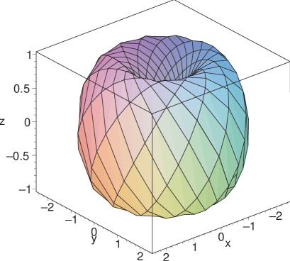
Figure 1: Stereographic projection of the solution $T=T(u)$ of section 3.1.

In this stereographic projection, the configuration obtained as the thin limit of the solution (3.29) is visualized as in Fig. 2. Note that the figure is obtained after patching all contributions from the four delta functions in (3.32). At first, the shape of the surface in Fig. 2 does not look like a torus. However, the spatial infinities of R³ are to be identified in the stereographic projection and it is not difficult to see that the surface actually is a torus embedded in S³. Indeed, with the new coordinates

$$\zeta^{\prime}_{1} = -\frac{1}{\sqrt{2}}(\zeta_{2}+\zeta_{4}),$$

$$\zeta^{\prime}_{2} = \frac{1}{\sqrt{2}}(\zeta_{1}+\zeta_{3}),$$

$$\zeta^{\prime}_{3} = \frac{1}{\sqrt{2}}(\zeta_{2}-\zeta_{4}),$$

$$\zeta^{\prime}_{4} = \frac{1}{\sqrt{2}}(\zeta_{1}+\zeta_{3}),$$ (A.3)

and the corresponding stereographic projection, the surface in Fig. 2 is precisely transformed to the torus of Fig. 1.

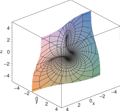
Figure 2: Stereographic projection of the solution $T=T(w)$ of section 3.2.

References

- [1] For a review, see A. Sen, “Tachyon dynamics in open string theory,” arXiv:hep-th/0410103, and references therein.
- [2] A. Sen, “Rolling tachyon,” JHEP 0204, 048 (2002) [arXiv:hep-th/0203211]; “Tachyon matter,” JHEP 0207, 065 (2002) [arXiv:hep-th/0203265].
- [3] E. Witten, “D-branes and K-theory,” JHEP 9812, 019 (1998) [arXiv:hep-th/9810188].
- [4] A. Sen, “Field theory of tachyon matter,” Mod. Phys. Lett. A 17, 1797 (2002) [arXiv:hep-th/0204143].
- [5] A. Sen, “Dirac-Born-Infeld action on the tachyon kink and vortex,” Phys. Rev. D 68, 066008 (2003) [arXiv:hep-th/0303057].
- [6] M. Cvetic, G. W. Gibbons and C. N. Pope, “A string and M-theory origin for the Salam-Sezgin model,” Nucl. Phys. B 677, 164 (2004) [arXiv:hep-th/0308026].
- [7] A. Salam and E. Sezgin, “Chiral compactification on Minkowski X S**2 of N=2 Einstein-Maxwell supergravity in six-dimensions,” Phys. Lett. B 147, 47 (1984).
- [8] D. Kutasov, “D-brane dynamics near NS5-branes,” arXiv:hep-th/0405058.
- [9] C. G. Callan, J. A. Harvey and A. Strominger, “Supersymmetric string solitons,” arXiv:hep-th/9112030.
- [10] S. J. Rey, “The Confining Phase Of Superstrings And Axionic Strings,” Phys. Rev. D 43, 526 (1991).
- [11] C. Kim, Y. Kim and C. O. Lee, “Tachyon kinks,” JHEP 0305, 020 (2003) [arXiv:hep-th/0304180]; C. Kim, Y. Kim, O. K. Kwon and C. O. Lee, “Tachyon kinks on unstable Dp-branes,” JHEP 0311, 034 (2003) [arXiv:hep-th/0305092].
- [12] T. Okuda and S. Sugimoto, “Coupling of rolling tachyon to closed strings,” Nucl. Phys. B 647, 101 (2002) [arXiv:hep-th/0208196].
- [13] N. Lambert, H. Liu and J. Maldacena, “Closed strings from decaying D-branes,” arXiv:hep-th/0303139.
- [14] M. R. Garousi, “Tachyon couplings on non-BPS D-branes and Dirac-Born-Infeld action,” Nucl. Phys. B 584, 284 (2000) [arXiv:hep-th/0003122]; E. A. Bergshoeff, M. de Roo, T. C. de Wit, E. Eyras and S. Panda, “T-duality and actions for non-BPS D-branes,” JHEP 0005, 009 (2000) [arXiv:hep-th/0003221]; J. Kluson, “Proposal for non-BPS D-brane action,” Phys. Rev. D 62, 126003 (2000) [arXiv:hep-th/0004106].
- [15] A. Buchel, P. Langfelder and J. Walcher, “Does the tachyon matter?,” Annals Phys. 302, 78 (2002) [arXiv:hep-th/0207235]; C. Kim, H. B. Kim, Y. Kim and O-K. Kwon, “Electromagnetic string fluid in rolling tachyon,” JHEP 0303, 008 (2003) [arXiv:hep-th/0301076].
- [16] C. Kim, Y. Kim, O-K. Kwon and P. Yi, “Tachyon tube and supertube,” JHEP 0309, 042 (2003) [arXiv:hep-th/0307184].
- [17] C. Kim, Y. Kim and O. K. Kwon, “Tubular D-branes in Salam-Sezgin Model,” JHEP 0405, 020 (2004) [arXiv:hep-th/0404163].
- [18] K. Okuyama, “Wess-Zumino term in tachyon effective action,” JHEP 0305, 005 (2003) [arXiv:hep-th/0304108].