Spacetime structure of static solutions in Gauss-Bonnet gravity: neutral case
Abstract
We study the spacetime structures of the static solutions in the -dimensional Einstein-Gauss-Bonnet- system systematically. We assume the Gauss-Bonnet coefficient is non-negative and a cosmological constant is either positive, zero, or negative. The solutions have the -dimensional Euclidean sub-manifold, which is the Einstein manifold with the curvature and . We also assume , where is the curvature radius, in order for the sourceless solution () to be defined. The general solutions are classified into plus and minus branches. The structures of the center, horizons, infinity and the singular point depend on the parameters , , , and branches complicatedly so that a variety of global structures for the solutions are found. In our analysis, the - diagram is used, which makes our consideration clear and enables easy understanding by visual effects. In the plus branch, all the solutions have the same asymptotic structure at infinity as that in general relativity with a negative cosmological constant. For the negative mass parameter, a new type of singularity called the branch singularity appears at non-zero finite radius . The divergent behavior around the singularity in Gauss-Bonnet gravity is milder than that around the central singularity in general relativity. There are three types of horizons: an inner, black hole, and cosmological. In the cases the plus-branch solutions do not have any horizon. In the case, the radius of the horizon is restricted as () in the plus (minus) branch. The black hole solution with zero or negative mass exists in the plus branch even for the zero or positive cosmological constant. There is also the extreme black hole solution with positive mass in spite of the lack of electromagnetic charge. We briefly discuss the effect of the Gauss-Bonnet corrections on black hole formation in a collider and the possibility of the violation of third law of the black hole thermodynamics.
pacs:
04.50.+h, 04.65.+e, 04.70.-sI Introduction
Black holes are characteristic objects to general theory of relativity. Recent observational data show the existence of one or more huge black holes in the central region of a number of galaxies. While over the past decades much concerning the nature of black hole spacetimes has been clarified, a good many unsolved problems remain. One of the most important ones is what the final state of black-hole evaporation through quantum effects is. The mid-galaxy supermassive black holes are certainly not related to this problem; however, it has been suggested that tiny black holes, whose quantum effect should not be neglected, could be formed in the early universe by the gravitational collapse of the primordial density fluctuations. Black holes may become small enough in the final stage of evaporation enough for quantum aspects of gravity to become noticeable. In other words, such tiny black holes may provide a good opportunity for learning not only about strong gravitational fields but also about of the quantum aspects of gravity.
Up to now many quantum theories of gravity have been proposed. Among them superstring/M-theory formulated in the higher dimensional spacetime is the most promising candidate. So far, however, no much is known about the non-perturbative aspects of the theory have not been To take string effects perturbatively into classical gravity is one approach to the study of the quantum effects of gravity.
A recent and attractive proposal for a new picture of our universe called the braneworld universe large ; Randall ; DGP is based on superstring/M-theory Lukas . According to these we live on a four-dimensional timelike hypersurface embedded in a higher-dimensional bulk spacetime. Because the fundamental scale could be around TeV scale in this scenario, these models suggest that creation of tiny black holes in a linear hadron collider is possible Bhformation . From this point of view, the investigation of the string effects on the black holes is important.
In this paper we consider the -dimensional action with the Gauss-Bonnet terms for gravity GB , which we call Gauss-Bonnet gravity hereafter, as the higher curvature corrections to general relativity. The Gauss-Bonnet terms naturally arise as the next leading order of the -expansion of superstring theory, where is inverse string tension Gross , and are ghost-free combinations Zwie . The black hole solutions in Gauss-Bonnet gravity were first discovered by Boulware and Deser GB_BH and Wheeler Wheeler_1 , independently. Since then many types of black hole solutions have been intensively studied Torii . The black hole solutions with a cosmological constant were investigated in several papers Cho ; Cvetic ; Cai ; Neupane ; Cai2 . In the system with a negative cosmological constant, black holes can have horizons with non-spherical topology such as torus, hyperboloid, and other compactified sub-manifolds. These solutions were originally found in general relativity and are called topological black holes Brown . They are distinctive in that there exist zero-mass and negative mass black hole solutions, and in both cases their properties were investigated Cai3 . Topological black hole solutions have also been studied in Gauss-Bonnet gravity Cho ; Cvetic ; Cai ; Neupane . Black hole solutions in more general Lovelock gravity Lovelock have also been investigated Myers ; Whitt
In Gauss-Bonnet gravity, there are two kinds of black hole solutions, which are classified into the plus and the minus branches. When Boulware and Deser first discovered the solutions, they claimed that the vacuum state in one of the branches (the plus branch in our definition) are unstable GB_BH , so that the solutions in the minus branch have been intensively investigated, while less attention has been paid to the solutions in the plus branch. However, the vacuum states in both branches have recently turned out to be stable Deser . Moreover, it is known that the solutions in five-dimensional Gauss-Bonnet gravity have qualitatively different properties from those of higher-dimensions. There is, however, a lack of detailed investigations of the five-dimensional case.
In this paper, we extend the previous work and give a unified viewpoint on the black hole solutions in Gauss-Bonnet gravity. We include all the aforementioned cases, i.e., the plus and the minus branches, five- and higher-dimensional cases. In particular, we focus on the global structure of the spacetime. We also consider the case with a positive/negative cosmological constant and that with a sub-manifold with non-spherical topology. We investigate not only the black hole solutions but also other kinds of solutions, such as regular or globally naked solutions.
In Sec. II, we introduce our model and show solutions that are generalizations of Boulware and Deser’s original. In Sec. III, we review the solutions in the Einstein- system for comparison. In Sec. IV, the general properties of the solutions in the Einstein-Gauss-Bonnet- system with , whose meaning is given in the text, are investigated. In Sec. V, we show the - diagram and study the number of horizons for each solution. The global structures of the solution are summarized in tables. Sec. VI is devoted to the analysis of the special case where . In Sec. VII, we give conclusions and discuss related issues and future work. Throughout this paper we use units such that . As for notation and conversion we follow Ref. Gravitation . The Greek indices run , .
II Model and solutions
We start with the following -dimensional () action:
| (1) |
where and are the -dimensional Ricci scalar and the cosmological constant, respectively. , where is the -dimensional gravitational constant. The Gauss-Bonnet Lagrangean consists of the Ricci scalar, the Ricci tensor, and the Riemann tensor as
| (2) |
This set of terms is called the Gauss-Bonnet terms. In the four-dimensional case, the Gauss-Bonnet terms do not appear in the equation of motion but contribute only as the surface terms. As a result, the model becomes ordinary Einstein theory with a cosmological constant. is the coupling constant of the Gauss-Bonnet terms. This type of action is derived from superstring theory in the low energy limit Gross . In such cases is related to the inverse string tension and is positive definite. Since the Minkowski spacetime becomes unstable for negative , we consider only the case in this paper. is the action of matter fields.
The gravitational equation of the action (1) is
| (3) |
where
| (4) | |||||
| (5) | |||||
Since we are interested in vacuum solutions in this paper, the energy-momentum tensor is set at zero.
We assume a static spacetime and adopt the following line element:
| (6) |
where is the metric of the -dimensional Einstein space .
In the four-dimensional case, the Einstein space is two-dimensional. By taking to be complete, we can write it as a quotient space , where the universal covering space is either two-sphere , two-torus or two-hyperboloid , and is a freely and properly discretely acting subgroup of the isometry group of . If the action of on is nontrivial, is multiply connected. For concrete examples, see Ref. Wolf . In the five-dimensional case, i.e., the case in which the sub-manifold is the three-dimensional Einstein space, the situation is almost the same 3-einstein_2 . In the higher-dimensional cases, the -dimensional () Einstein space has rich structures and is not necessarily homogeneous, i.e., it can even have non-constant curvature 3-einstein_1 .
The and components of the gravitational equation (3) give , where the prime denotes a derivative with respect to . By rescaling the time coordinate suitably, we can always set
| (7) |
without loss of generality.
The equation of the metric function is written as
| (8) |
where and . In our definition, a negative (positive) gives a positive (negative) . is the curvature of the -dimensional Einstein space and takes (positive curvature), (flat), and (negative curvature). This equation is integrated to give the general solution as
| (9) |
where
| (10) |
The integration constant is proportional to the mass of a black hole for black hole spacetime. Although we will also consider solutions which are not black holes, we call the mass of the solution. is the volume of the unit -dimensional Einstein space. For example, for the -dimensional sphere , where is the gamma function. There are two families of solutions that correspond to the sign in front of the square root in Eq. (9). We call the family with a minus (plus) sign the minus- (plus-) branch solution. By introducing new variables as , , and , the curvature radius is scaled out when the cosmological constant is non-zero. In the case, it is convenient to rescale the variables by as and .
The global structure of the spacetime is characterized by the properties of the singularities, horizons, and infinities. A horizon is a null hypersurface defined by such that with finite curvatures, where is a constant horizon radius. In this paper, we call a horizon on which a black hole horizon Penrose . If there is a horizon inside of a black hole horizon and if it satisfies , we call it an inner horizon. If a horizon satisfies and if it is the outermost horizon, we call it a cosmological horizon. We call a horizon on which a degenerate horizon. Among them if the first non-zero derivative coefficient is positive, i.e., and for any , , we call it a degenerate black hole horizon. A solution with degenerate horizons is called extreme. The solutions in this paper are classified into three types by the existence of the horizons. The first one is a black hole solution that has a black hole horizon. A solution that does not have a black hole horizon but does have a locally naked singularity is a globally naked solution. This is the second type. The last type is a singularity-free solution without a black hole horizon, which we call a regular solution.
Since there are many parameters in our solutions, such as , (or ), , and branches, the analysis should be performed systematically. In this paper we employ a - diagram, which we explain below.
First we choose one of the branches, and fix the values of , , and . Then the solutions are parametrized by one parameter, . By changing the mass parameter of the solutions, we can plot the location of the singularity and horizons on the - diagram. These plots form a number of curves. The curve of the horizon radius may be a multi-valued function of , which means that there exist several horizons in the spacetime, such as a black hole, an inner, and a cosmological horizon. This diagram shows the number and location of the horizons and singularities for each . In several cases the curve of the horizon radius becomes vertical where two types of horizon coincide. The solution at any such vertical point is extreme. Next, when we vary other parameters, say , the curves on the - diagram slide a bit from the original one. When there is an extreme solution in the family of the solutions, we obtain the curve for the extreme solution on the - diagram by joining points for extreme solutions in each . We will show concrete examples of the - diagram in general relativity in the next section.
All the solutions at vertical points of the - curve are not extreme solutions. Let us make the relation clear between the vertical points and the extreme solutions. When , , and are fixed, the metric function is a function of with one parameter . Then let us define a new function , where the right-hand side (rhs) is evaluated with the mass parameter . The - curve is obtained by the constraint condition . Then along the - curve, we find for . At the vertical point, . This implies that (i) and , or (ii) . The case (i) exemplifies the degenerate horizon condition. In the latter case (ii), however, one cannot be sure whether the horizon is degenerate or not. Then we should examine the condition directly. As we will see in the following sections, the latter case appears only when and , where is the radius of the branch singularity, defined in Sec. IV. The solution with or does not have a horizon but, instead, has a regular or a singular point at . As a result, only the case (i) produces a degenerate horizon. In fact, however, several solutions exist with and , both in general relativity and Gauss-Bonnet theory. We call this type of horizon an almost degenerate horizon. These infinitesimally small black hole solutions may be important from the thermodynamical point of view because their temperature is also infinitesimally small and affects the evolution of the black hole. If , we find also , and the horizon is degenerate. Details in general relativity and Gauss-Bonnet cases will be discussed in each section.
III Static solutions in the Einstein- system
Before investigating the system with the Gauss-Bonnet terms, we first review the spacetime structure of the static solutions described by the metric form (6) in the Einstein- system using the - diagram for comparison.
By taking the limit of , Gauss-Bonnet gravity reduces to general relativity. In this limit,
| (11) |
is obtained only for the minus branch of Eq. (9), while there is no such limit for the plus branch. The spacetime is described by Eqs. (6), (7), and (11). We do not consider the case with , in which the function is identically zero.
There is a curvature singularity at the center () except for the case with . Around the center, the Kretschmann invariant behaves as follows:
| (12) | |||||
Whether the central singularity is spacelike, null, or timelike depends on the dominant term of Eq. (11) for . When (), the metric function (), and the tortoise coordinate defined by
| (13) |
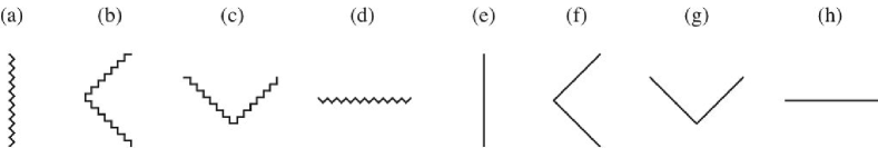
is finite at the center. So the singularity is spacelike (Fig. 1(d)) (timelike (Fig. 1(a))). When and (), the center is regular regular and timelike (Fig. 1(e)) (spacelike (Fig. 1(h))), while it becomes null for and because (Fig. 1(f) for and Fig. 1(g) for ).
The structure of infinity depends on the dominant term of Eq. (11) for . When there is a non-zero cosmological constant, the dominant term is . When (), the spacetime asymptotically approaches the de Sitter (dS) (anti-de Sitter (adS)) spacetime, of which region is expressed by the conformal diagram Fig. 2(d) (Fig. 2(b)). The second leading term is the curvature term . If and , the spacetime is asymptotically flat, of which region is expressed by the conformal diagram Fig. 2(i). If and , the conformal diagram of infinity is Fig. 2(iii). When , the term is dominant. For (), infinity is expressed by Fig. 2(iii) (Fig. 2(i)).
Since the number of the horizons depends complicatedly on parameters such as mass, the cosmological constant, and so on, the - diagram is useful. From Eq. (11), the - relation in the Einstein- system is
| (14) |
We consider here that the values of and are fixed, so that this relation becomes a curve on the - diagram.
On the - curve there are some points that are physically important. For example, points where the curve terminates at a singularity, points where the value of becomes zero, and points where the curve becomes vertical. From the degeneracy condition of the horizon , where is the radius of the degenerate horizon, we can show that the - curve becomes vertical at this point. However, the inverse is not always true, as we showed in Sec. II. Let us examine the conditions (i) and (ii) in Sec. II in general relativity. By Eq. (11), . Except for , this equation becomes finite. Hence if the horizon radius at the vertical point on the - curve is non-zero, the horizon is degenerate. In the case, becomes zero by Eq. (14). If we set exactly, the physical center is not a horizon but a regular point. However, the analysis of the limiting solution , i.e., an infinitesimally small horizon, is important when we consider the evolution of the black hole. The condition of the degenerate horizon gives
| (15) |
In the case, for and for . Hence for the horizon of the vertical point with is the almost degenerate horizon, while it is not for .
The location and the mass parameter of the degenerate horizon are
| (16) | |||
| (17) |
respectively, for . The extreme solution exists when and have signs opposite to each other. When , these equations give and the solution is not an extreme solution but a regular solution. For , the degeneracy condition gives . This solution falls outside of our consideration. If is satisfied at the finite value of , the three horizons degenerate. However, there is no such solution in the present system.
On the - diagram the extreme solution is expressed by the point where two horizons coincide. The diagram in Fig. 3 (d) is a typical example. This solution is the Schwarzschild-dS solution. The point E is where the curve becomes vertical. The solution at this point is the extreme solution and has the mass parameter . A solution with less mass has two horizons (a black hole and a cosmological horizons), and at the extreme point two horizons coincide. For the greater mass parameter, there is no horizon. In this manner, the number of the horizons changes at the mass parameter of the extreme solution like this. The number of the horizons also changes with the mass parameter at the points where the curve terminates in singularities, the value of becomes zero for a finite , and so on. We can see these points directly on the - diagram.
We will examine the number of horizons of the solutions by varying the mass parameter and show their spacetime structures in the cases of zero, positive, and negative cosmological constant, separately. The - diagrams are shown in Fig. 3 and the global structures of the solutions are summarized in Table 1.
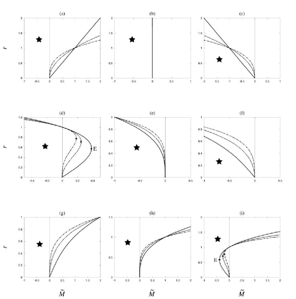
III.1 case
In the case, the solution is the -dimensional Schwarzschild solution. The - diagram is shown in Fig. 3(a). For , the solution has no horizon and represents the spacetime with a globally naked singularity. The solution with is the Minkowski spacetime note_1 . For , the solution has a single horizon at and represents the Schwarzschild black hole spacetime.
In the case, the - diagram is shown in Fig. 3(b). The - relation becomes . However, since we do not consider the case, there is no - curve in this diagram. For , the solution has no horizon and represents the spacetime with a globally naked singularity.
In the case, the - diagram is shown in Fig. 3(c). For , the solution has a cosmological horizon and represents the spacetime with a globally naked singularity. For , the solution is regular hyperbolic spacetime. For , the solution has no horizon and represents the spacetime with a globally naked singularity.
III.2 case
In the case, the solution is the Schwarzschild-dS solution. The - diagram is shown in Fig. 3(d). There is an extreme solution with mass given by Eq. (17). For , the solution has a cosmological horizon and represents the spacetime with a globally naked singularity. For , the spacetime is the -dimensional dS spacetime, which has a cosmological horizon at . For , there are a black hole and a cosmological horizons and the solution represents the Schwarzschild-dS black hole spacetime. For , the black hole and the cosmological horizons coincide, and the horizon is degenerate. The location of the degenerate horizon is given by Eq. (16). For , the solution has no horizon and represents the spacetime with a globally naked singularity.
In the case, the - diagram is shown in Fig. 3(e). For , the solution has a cosmological horizon and represents the spacetime with a globally naked singularity. The derivative of the metric function vanishes in the zero horizon limit, i.e., as . This implies that the horizon almost degenerates in this limit. For , the solution has no horizon and represents the regular spacetime. For , the solution has no horizon and represents the spacetime with a globally naked singularity.
In the case, the - diagram is shown in Fig. 3(f). For , the solution has a cosmological horizon and represents the spacetime with a globally naked singularity. For , the solution has no horizon and represents the regular spacetime. For , the solution has no horizon and represents the spacetime with a globally naked singularity.
III.3 case
When the curvature of the -dimensional Einstein space is or , there is no black hole solution in the zero or positive cosmological constant case. However, the negative cosmological constant allows such black hole solutions. They are called topological black holes Brown ; Cai3 and show remarkable properties in that the mass of such solutions can be negative.
In the case, the solution is the -dimensional Schwarzschild-adS solution. The - diagram is shown in Fig. 3(g). For , the solution has no horizon and represents the spacetime with a globally naked singularity. For , the solution has no horizon and represents the everywhere regular spacetime. The spacetime is the adS spacetime. For , the solution has one black hole horizon and represents the Schwarzschild-adS black hole spacetime.
In the case, the - diagram is shown in Fig. 3(h). For , the solution has no horizon and represents the spacetime with a globally naked singularity. For , the solution has no horizon; the spacetime has a regular null center. For , the solution has one black hole horizon. In the infinitesimally small horizon limit , the horizon is almost degenerate.
Where , the case is quite different from the others. The black hole solution with zero or negative mass can exist. The - diagram is shown in Fig. 3(i). There is an extreme solution which has the lowest mass of all the black hole solutions in this system:
| (18) |
The degenerate horizon locates at
| (19) |
For , the solution has no horizon and represents the spacetime with a globally naked singularity. For , the solution has a degenerate horizon and represents the extreme black hole spacetime. For , the solution has an inner and a black hole horizons and represents the black hole spacetime with negative mass. For , the solution has regular center and a black hole horizon at . The spacetime is black hole spacetime with zero mass. It should be noted again that the term “regular” in this paper means that the Kretschmann invariant does not diverge. So the “regular” point can be singular by the topological origin of the -dimensional Einstein space. The center of the zero mass black hole is this case. For , the solution has a black hole horizon and represents the black hole spacetime.
IV General properties of solutions in the Einstein-Gauss-Bonnet- system
Next we proceed to the cases of Gauss-Bonnet gravity. Let us discuss the general properties of the static solutions in this system.
In the case of , the metric function is
| (20) |
For a well-defined theory, the following condition should be satisfied:
| (21) |
Although any non-negative value of satisfies this condition in the zero and positive cosmological constant cases, it is restricted as where the cosmological constant is negative. In this section, we assume . The special case where will be investigated in Sec. VI separately.
From Eq. (20), the effective curvature radius is defined by
| (22) |
The sign of the square of the effective curvature radius is the same as in the minus branch, while is always positive independent of in the plus branch. Hence the spacetime approaches the adS spacetime for asymptotically in the plus branch for even when the pure cosmological constant is positive. In Sec. III, we showed the structure of the infinity of the solutions, which in the Einstein- system depends on the value of . By replacing in the discussion in the Einstein- system by , the structure of infinity in the Einstein-Gauss-Bonnet- system is obtained.
Besides the central singularity at , there can be another singularity at called the branch singularity. is obtained by the condition that the inside of the square root of Eq. (9) vanishes, and the - relation becomes
| (23) |
Around the branch singularity the Kretschmann invariant behaves as
| (24) |
By the condition Eq. (21), there are no positive real roots when , while one positive root exists for . decreases monotonically as increases and approaches zero in the limit of .
When a branch singularity exists, the metric function behaves around it as
| (25) |
Hence if or , the singularity is timelike (Fig. 1(a)). When , the singularities are timelike and spacelike (Fig. 1(d)) for and , respectively. In the special case where and , the singularities are spacelike and timelike for the minus and plus branches, respectively.
The positive-mass solutions have a central singularity. Here the metric function behaves
| (26) |
around the center. Hence if , the singularity is spacelike (timelike) for the minus (plus) branch. The Kretschmann invariant behaves as
| (27) |
Although is finite when , the Kretschmann invariant behaves as
| (28) |
so that the center is singular. In the minus branch, the singularity is spacelike when and . When , the singularity is spacelike for , null (Fig. 1(b)) for , and timelike for . In the plus branch, the singularity is timelike when and . When , the singularity is spacelike for , null for , and timelike for . It is noted that the divergent behavior of the central singularity in Gauss-Bonnet gravity is milder than that in general relativity (see Eqs. (12) and (27)). It is also noted that the divergent behavior of the branch singularity is milder than that of the central singularity (see Eqs. (24) and (27)).
For the solution with zero mass, the center is regular. Since the metric function is described as , the conformal diagram around the center is obtained by replacing in the discussion in the Einstein- system by .
From the condition of the horizon , we find
| (29) |
Hence
| (30) | |||
| (31) |
so that we can conclude that solutions in the plus branch have no horizon for . Hence the solutions represent the spacetime with a globally naked singularity except for the solution with . When , the horizon radius is restricted as in the plus branch, while in the minus branch, the horizon has the lower limit . There are no such restrictions for and .
The - relation is
| (32) |
For this relation is same as that in general relativity Eq. (14). For the solution with has a branch singularity at , where
| (33) |
This implies that the sequence of solutions is divided by the branch singularity into the plus and the minus branches for . It is seen that the - curve in the - diagram terminates at the - curve just at the point with (Point B in Figs. 4 and 5). For the other mass parameter , the horizon radius is always larger than that of the branch singularity. In the limit of , the mass of the solution vanishes in the case, while it approaches in five-dimensions.
In general relativity there are some extreme black hole solutions with a degenerate horizon. The Gauss-Bonnet case has more variety. First let us examine the relation of a vertical point in the - curve and an extreme solution. By Eq. (9), except for and . Hence the horizon of the vertical point is degenerate for the and cases. In the case, for in and for any in , and the horizon is almost degenerate, while for in , and the horizon is not degenerate. In the case, for any and the horizon is not degenerate.
The radius of the degenerate horizon is
| (34) |
for , and
| (35) |
for . Note that the sign does not correspond to the sign of the solution branches. The mass of the extreme solution is
| (36) |
We denote the mass of the extreme solution and the radius of its degenerate horizon in the plus (minus) branch as and ( and ), respectively. In the and case, must be negative by the positivity of the degenerate horizon. Since , the extreme solution belongs to the plus branch. In the case, the minus sign should be taken in Eq. (34), and the extreme solutions appear in both and cases. In the case, must be negative, and then both signs in Eq. (34) give extreme solutions. Although the black hole solution with a degenerate horizon necessarily has negative mass in general relativity (in the and case), the extreme black hole solutions in the cases have positive mass.
In five-dimension the rhs of Eq. (35) vanishes, and there is no extreme solution in the case. For (), must be positive (negative) and the minus (plus) sign should be assumed in Eq. (34). The radius of the degenerate horizon does not depend on , and Eq. (34) gives the same expression as that in the Einstein- system. This implies that a degenerate horizon appears at the same radius as that in the Einstein- system. However, the mass of the extreme solution depends on , and the - relation shows a line on the - diagram, as we will see in the next section.
The topological black hole solutions in general relativity can have a zero or a negative mass parameter. Since the minus-branch solutions approach the solutions in general relativity in the limit, it is expected that such solutions with zero or negative mass exist also in the Gauss-Bonnet case. Furthermore, similar solutions appear in the plus branch. When the cosmological constant is zero, the horizon radius of the massless solution is
| (37) |
from Eq. (32). There is one positive real root in the plus branch for . This is a black hole horizon. In the cases, the horizon radius of the massless solution is given as
| (38) |
The sign does not mean the branches. When , has two positive real roots for , one of which is in the plus branch while the other is in the minus branch, while there are not such solutions for and . Both horizons are black hole horizons. When , has one positive real root in the minus branch for and in the plus branch for . The former corresponds to the conventional cosmological horizon in dS spacetime. The latter is, however, the black hole solution, as we will see later. Hence there are zero mass black hole solutions even in the zero and positive cosmological constant cases. This type of solution does not exist in general relativity with but appears if the Gauss-Bonnet effects are considered.
V - diagram and spacetime structure
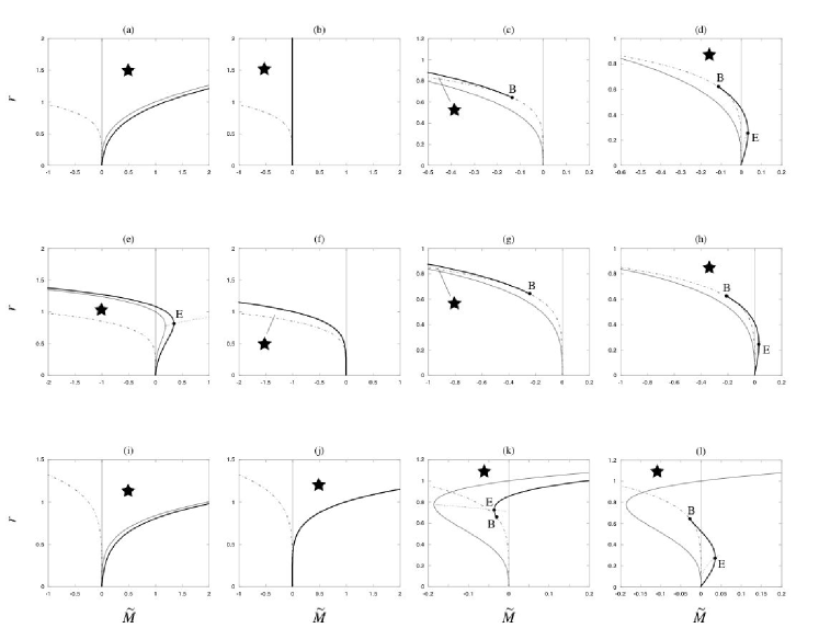
In the previous section, we discussed properties of the singularity, infinity, and horizons of the solutions in the Einstein-Gauss-Bonnet- system. In this section we examine the number of horizons and show the spacetime structures of the solutions by taking into account the above properties. As an aid to discussion, the - diagrams are shown in Fig. 4 () and Fig. 5 (). The spacetime structures of the solutions are summarized in Tables 2 () and 3 (). Since the spacetime structures in 5-dimension are different from those in the case, we separate the tables.
V.1 case
V.1.1 case
When , a solution in the plus branch has no horizon and represents the spacetime with a globally naked singularity unless . The spacetime with is the -dimensional adS spacetime whose curvature radius is .
In the case, the - diagram of the minus branch is shown as in Fig. 4(a). For , the solution has no horizon, and the branch singularity can be seen from infinity. The solution represents the spacetime with a globally naked singularity. For , the solution has a regular center, and the spacetime is Minkowski spacetime. For , the solution has a black hole horizon and represents the -dimensional Schwarzschild-adS black hole spacetime.
In the case, the - diagram of the minus branch is shown as in Fig. 5(a). For , the diagram is qualitatively the same as that in the higher-dimensional case. For the solution has no horizon and represents the spacetime with a globally naked singularity. For the solution has a black hole horizon and represents the five-dimensional Schwarzschild-adS black hole spacetime. In the limit, the black hole horizon is almost degenerate.
V.1.2 case
When , a solution in the plus branch has no horizon and represents the spacetime with a globally naked singularity unless .
The - diagrams of the minus branch are shown in Figs. 4(b) and 5(b). No horizon exists in the minus branch either, and every solution represents the spacetime with a globally naked singularity. For , there is a branch singularity at . For , there is a central singularity at . In the whole region the signature of spacetime changes, i.e., the Killing vector is spacelike for . We call this type of region a trapped region.
V.1.3 case
In the , the solution in the plus branch can have a horizon. First, however, let us consider a solution in the minus branch. The - diagrams are shown in Figs. 4(c) and 5(c). The diagrams in and higher dimensional cases are qualitatively the same. For , the solution has only a cosmological horizon and represents the spacetime with a globally naked singularity. For , the solution has no horizon and represents the spacetime with a globally naked singularity. For , the solution has no horizon and represents the regular spacetime. However, the signature of spacetime is opposite to that in the ordinary untrapped region. For , the solution has no horizon and represents the spacetime with a globally naked singularity. The signature of spacetime is opposite to that in the ordinary untrapped region.
In the case, the - diagram of the plus branch is shown as in Fig. 4(d). For , the solution has no horizon and represents the spacetime with a globally naked singularity. For , the solution has a black hole horizon. It should be noted that the negative mass black hole solution can exist without a cosmological constant. For , the solution has a black hole horizon and represents black hole spacetime. This solution is the zero mass black hole. For , the solution has two horizons, which are black hole and inner horizons. Hence the spacetime structure is similar to the RN-adS black hole spacetime, even though the solution is neutral. In general relativity the negative mass black hole solution always has an inner horizon, while this solution only has a black hole horizon. For , the solution has a degenerate horizon and represents the extreme black hole spacetime. For , the solution has no horizon and represents the spacetime with a globally naked singularity.
In the case, the - diagram of the plus branch is as shown in Fig. 5(d). For , the diagram is qualitatively the same as that in the higher-dimensional case. For , the solution has a black hole horizon. In the limit, the black hole horizon is almost degenerate. For , the solution has no horizon and represents the spacetime with a globally naked singularity.
V.2 case
V.2.1 case
When , there is no horizon in the plus branch, and the spacetime has a globally naked singularity unless . The solution with is the -dimensional dS spacetime.
In the case, the - diagram of the minus branch is shown as in Fig. 4(e). There is one extreme solution with mass for fixed . For , there is a cosmological horizon and represents the spacetime with a globally naked singularity. For , the solution has a regular center and a cosmological horizon. The spacetime is the -dimensional dS spacetime whose curvature radius is . For , the solution has a black hole and a cosmological horizons. The spacetime is the -dimensional Schwarzschild-dS spacetime. For , the solution has a degenerate horizon and represents the extreme black hole spacetime. For , the solution has no horizon and represents the spacetime with a globally naked singularity.
In the case, the - diagram of the minus branch is shown in Fig. 5(e). The diagram is qualitatively the same as that in the higher dimensional case except for the mass parameter range . For , the solution has a cosmological horizon and represents the spacetime with a globally naked singularity. In the limit, the black hole horizon is almost degenerate.
V.2.2 case
When , there is no horizon in the plus branch, and the spacetime has a globally naked singularity unless .
The - diagram of the minus branch is shown in Figs. 4(f) and 5(f). For , the solution has a cosmological horizon and represents the spacetime with a globally naked singularity. In the limit, the cosmological horizon is almost degenerate. For , the solution has no horizon and represents the regular spacetime. However, the spacetime is trapped. For , the solution has no horizon and represents the spacetime with a globally naked singularity.
V.2.3 case
The - diagrams of the minus branches are shown in Figs. 4(g) and 4(h) for , and in Figs. 5(g) and 5(h) for . They are same as those for and qualitatively. Hence the classification of the number of the horizons is same. However, since the structure of infinity in the minus-branch solution differs according to whether or , the spacetime structures shown in Tables 2 and 3 differ.
V.3 case
V.3.1 case
When , there is no horizon in the plus branch, and the solution has a globally naked singularity unless . The spacetime with is the -dimensional adS spacetime.
In the case, the - diagram in the minus branch is shown in as Fig. 4(i). For , the solution has no horizon and represents the spacetime with a globally naked singularity. For , the solution has no horizon and represents the -dimensional adS spacetime. For , the solution has a black hole horizon and represents the -dimensional Schwarzschild-adS black hole.
In the case, the - diagram of the minus branch is shown as in Fig. 5(i). The diagram is qualitatively the same as that in the higher-dimensional case except for the mass parameter range . For , the solution has no horizon and represents the spacetime with a globally naked singularity. In the limit, the black hole horizon is almost degenerate.
V.3.2 case
When , there is no horizon in the plus branch, and the spacetime has a globally naked singularity unless .
The - diagram in the minus branch is shown in Fig. 4(j) for case and in Fig. 5(j) for . Both diagrams are qualitatively the same. For , the solution has no horizon and represents the spacetime with a globally naked singularity. For , the solution has no horizon and represents the regular spacetime. For , the solution has a black hole horizon. In the limit, the black hole horizon is almost degenerate.
V.3.3 case
In the case, has two positive roots by Eq. (34). It is easily seen that each extreme solution belongs to the minus and the plus branches, respectively. So we denote their radii as and with . It is enough to show that and . First let us compare with :
If the first term in the second line is larger than or equal to , the rhs of the equation is always positive. Hence we find . If not, the sign of the rhs is determined by the sum of the first two terms and the third term. Calculating
| (40) |
we find again the is less than . This implies that the extreme solution with belongs to the plus branch.
Next, let us show . Equation (34) implies that is the function of . monotonically increases as increases. For , the radius of the degenerate horizon is . This implies that for .
In the case, has only one positive root by Eq. (34). It is also shown in the similar way that the extreme solution belongs to the minus branch.
Let us consider a solution of the minus branch. The - diagrams are shown in Figs. 4(k) for case and 5(k) for case. The diagrams of and higher-dimensional cases are qualitatively the same. For , the solution has no horizon and represents the spacetime with a globally naked singularity. For , the solution has a degenerate horizon and represents the extreme black hole spacetime. For , the solution has a black hole and an inner horizons. For , there is a black hole horizon. This negative mass black hole solution has no inner horizon. For , the solution has a black hole horizon and a regular center. For , the solution has a black hole horizon.
In the case, the - diagram of the plus branch is shown as in Fig. 4(l). For , the solution has no horizon and represents the spacetime with a globally naked singularity. For , the solution has a black hole horizon. For , the solution has a black hole horizon and a regular center. For , the solution has a black hole and an inner horizons. For , the solution has a degenerate horizon and represents the extreme black hole spacetime. For , the solution has no horizon and represents the spacetime with a globally naked singularity.
In the case the - diagram in the plus branch is shown as in Fig. 5(l). The diagram is qualitatively the same as that in the higher-dimensional case except for the positive mass parameter range. For , the solution has a black hole horizon. For , the solution has no horizon and represents the spacetime with a globally naked singularity. In the limit, the black hole horizon is almost degenerate.
VI Einstein-Gauss-Bonnet- system: case
The system in which is a special case, where the plus and the minus branches coincide in the sourceless case . Since we have assumed that is positive, here only a negative is allowed. The metric function becomes
| (41) |
In the large radius the spacetime approaches the adS spacetime for with the effective curvature radius for .
The mass cannot be negative since the metric function takes a complex value. The boundary corresponds to the condition of the branch singularity for . In this sense it can be said that there is a branch singularity at in the - diagram. For , the solution is the adS spacetime when . For positive , there is a curvature singularity at , where the Kretschmann invariant behaves as
| (42) |
When , the singularity of the minus- (plus-) branch solution is spacelike (Fig. 1(iv)) (timelike (Fig. 1(i))). When , the structure of the singularity is as complicated as that where . In the minus branch, the singularity is spacelike when and . When , the singularity is spacelike for , null (Fig. 1(ii)) for , and timelike for . In the plus branch, the singularity is timelike when and . When , the singularity is spacelike for , null for , and timelike for .
Since the radius of a horizon is restricted to () for the plus (minus) branch, there are no horizons for solutions with in the plus branch. The - relation Eq. (32) becomes simple in form:
| (43) |
The - curve behaves as for , and for .
The relation between the vertical points of the - curve and extreme solutions is the same as that for . From the condition , the degenerate horizon appears as
| (44) |
for where . Because , the extreme solution appears only in the plus branch. The mass of the extreme solution is
| (45) |
The almost degenerate horizon appears in the limit for where and for any where .
When , the - diagrams are the same as those for qualitatively (Figs. 4(i), (j) and 5(i), (j)) except that negative mass solutions are forbidden. For , the solution has no horizon, and the spacetime is regular everywhere. The solution where is the adS solution whose curvature radius is . For , the solution has a black hole horizon. In the and/or case, the infinitesimally small black hole has an almost degenerate horizon.
When , the - diagram in the minus branch is shown as in Fig. 6(a). The negative mass range is forbidden. For , the solution has a black hole horizon, and the spacetime is regular everywhere. For , the solution has a black hole horizon. Even in the infinitesimally small mass limit, the horizon radius remains finite: .
The - diagram in the plus branch for is shown in Fig. 6(b). In the case, there is one extreme solution where mass and radius are given by Eqs. (45) and (44), respectively. For , the solution has a black hole horizon and represents the regular spacetime. For , the solution has an inner and a black hole horizons and represents the black hole spacetime. For , the solution has a degenerate horizon and represents the extreme black hole spacetime. For , the solution has no horizon and represents the spacetime with a globally naked singularity. In the case, there is no extreme solution. For , the solution has a black hole horizon, and the spacetime is regular everywhere. For , the solution has a black hole horizon, represents the black hole spacetime. In the limit, the horizon is almost degenerate. For , the solution has no horizon and represents the spacetime with a globally naked singularity. The spacetime structures of these solutions are summarized in Table 4.
VII Conclusions and Discussion
We have studied spacetime structures of the static solutions in the -dimensional Einstein-Gauss-Bonnet- system systematically. We assume that the Gauss-Bonnet coefficient is non-negative. This assumption is consistent with the low energy effective action derived from superstring/M-theory. The solutions we considered in this paper have the -dimensional Euclidean sub-manifold, which is the Einstein, for example, sphere, flat, or hyperboloid. When the curvature of the sub-manifold is , black holes are called topological black holes. We assume in order for the sourceless solution () to be defined. There is no solution with a negative mass parameter when . The structures of the center, horizons, asymptotic regions, and the singular point depend on the parameters , , , , and branches complicatedly so that a variety of global structures for the solution are found. In our analysis, an - diagram is used on which the -, - and - curves are drawn. It makes our consideration clear and enables easy understanding through visual effects. The solutions are classified into regular, black hole and globally naked solutions.
In Gauss-Bonnet gravity, the general solutions, which were first obtained by Boulware and Deser for the vanishing cosmological constant and for , are classified into the plus and the minus branches. In the limit, the solution in the minus branch recovers the one in general relativity, while there is no solution in the plus branch. In general relativity, the behavior of is dominated by the cosmological constant, and the asymptotic structure of a solution is generally determined by that term. In Gauss-Bonnet gravity, the curvature radius in general relativity is replaced by the effective curvature radius . In the minus branch the signs of and are same, and the ordinary correspondence between the signs of the cosmological constant and the asymptotic structures is obtained. In the plus branch, however, the signs of are always positive independently of the cosmological constant, and all the solutions have the same asymptotic structure as that in general relativity with a negative cosmological constant.
For the positive mass parameter, the singularity exists at the center. There the Kretschmann invariant behaves as . For the negative mass parameter, the new type of singularity called the branch singularity appears at non-zero finite radius . There the Kretschmann invariant behaves as . In any case, the divergent behavior in Gauss-Bonnet gravity is milder than the central singularity in general relativity .
Among the solutions in our analysis, the black hole solutions are the most important. There are three types of horizon: inner, black hole, and cosmological horizons. In the cases the plus branch solutions do not have any horizon. In the case, the radius of the horizon is restricted as () in the plus (minus) branch. The black hole solution in the plus branch for has interesting properties. In general relativity, the black hole solution with zero or negative mass appears only in the negative cosmological constant system, while such a solution exists in the plus branch even with the zero or positive cosmological constant in Gauss-Bonnet gravity. There are also the extreme black hole solutions with positive mass in spite of the lack of an electromagnetic charge.
For , the horizon radius of the black hole solutions in Gauss-Bonnet gravity is smaller than that in general relativity. Furthermore, in the case, the infinitesimally small black hole solution has a finite mass below which a black hole solution does not exist. This behavior would affect the black hole formation by a linear collider. Recent investigation of the higher-dimensional models represented by a braneworld model predicts such black hole formation if the fundamental energy scale is small enough. A rough estimate of these analyses is based on the Schwarzschild radius of the colliding particles. If their Schwarzschild radii calculated by the higher-dimensional model are comparable to the size of the colliding particles, a black hole will be formed. By taking into account the Gauss-Bonnet corrections, however, the Schwarzschild radius becomes small. This implies that the black hole formation occurs less frequently or not at all Rychkov .
Although we focus on the spacetime structure of the solutions in this paper, the thermodynamical properties of the black hole solution are important, in particular in the discussions of the evolution through Hawking radiation and final state of the black hole spacetime. The temperature of a black hole in Gauss-Bonnet gravity is obtained by the periodicity of the Euclidean time on the horizon by
| (46) |
In general relativity, the horizon radius of the black hole is related to the entropy of the black hole as . Since the temperature is from the first law of the black hole thermodynamics, a black hole with its horizon at the vertical point of the - curve where the horizon is degenerate has zero temperature. A solution with the almost degenerate horizon has infinitesimally small temperature. Although the expression of the entropy in Gauss-Bonnet gravity is different from that in general relativity, it is easy to show that the solution, at which the - curve becomes vertical on the diagram, where its horizon degenerates, has zero temperature. In Gauss-Bonnet gravity, entropy is not obtained by a quarter of the area of a black hole horizon. The second law of black hole thermodynamics would hold, while the area theorem would not. The relevant entropy of the system where the curvature terms exist in the action besides the Einstein-Hilbert action was proposed by Iyer and Wald, who regard it as the Noether charge associated with the diffeomorphism invariance Iyer . It is calculated as
| (47) |
in our model. is added to make the entropy non-negative Clunan .
In the case, a black hole solution with has the minimum mass . As the evaporation proceeds, the black hole loses its mass and its horizon radius shrinks to zero, and then the black hole seems to evolve to a naked singularity with the mass . However, since the temperature of the horizon becomes zero in this limit, we cannot be sure whether the black hole evaporates thoroughly and evolves to a singularity or not. Similar situations occur in the and case. We need detailed analysis of the evaporation process to clarify this issue.
Where and , the case is more interesting. There are black hole solutions both in the plus and the minus branches. In the minus branch, the black hole loses its mass, and the horizon radius becomes small through evaporation. As the solution approaches the extreme solution, evaporation becomes weak, and the black hole may evolve to the extreme solution in an infinite time. On the other hand, for the black hole solution in the plus branch, as the black hole loses its mass, the black hole horizon becomes large. Since the temperature of the black hole solution around the branch points B in Figs. 4 and 5 is non-zero, the black hole will evolve to a naked singularity that is not point-like but , rather, locates at . Conversely, the horizon area becomes small when matter is put into the black hole. This means that the area theorem in general relativity does not extend to Gauss-Bonnet gravity. However, it is confirmed that entropy increases in such a classical process, as is shown in Fig. 7. In general relativity there is an extreme limit of the Reissner-Nordström black hole. In this case, if we throw matter into the black hole, the ratio of the charge to the mass of the solution decreases, and it is impossible to make the solution extreme. If we continue to throw matter into our black hole, the solution will evolve to the extreme solution. As a result the mass exceeds that of the extreme solution, and the black hole becomes a naked singularity. This would be a violation of the third law of black hole thermodynamics.
As an important application of the solutions studied in this paper, it is known that the static black hole or the regular solutions with the metric of Eq. (6) can be used as a bulk spacetime in the braneworld cosmology. In the braneworld scenario, our universe is expressed by a shell in the higher-dimensional bulk spacetime. The radius of the shell in the bulk spacetime corresponds to the scale factor of our universe, so that the motion of the shell gives the evolution of the universe. In the Einstein-Maxwell- system, an infalling shell in the Reissner-Nordström bulk spacetime bounces at some finite radius RN-brane . This motion gives the bouncing universe without the big-bang singularity. However, this bounce occurs only inside of the inner horizon. As is well known, the inner horizon is unstable, so that the bouncing universe is hardly to be realized mass-inf ; kink . On the other hand, although there are several investigations of the braneworld in Gauss-Bonnet gravity GBbrane , much is not known. The bounce may occur outside of the inner horizon in Gauss-Bonnet gravity, so that a non-singular cosmology could be possible. These are under investigation Torii-brane .
Acknowledgements
We would like to thank Kei-ichi Maeda and Umpei Miyamoto for their discussion. This work was partially supported by a Grant for The 21st Century COE Program (Holistic Research and Education Center for Physics Self-Organization Systems) at Waseda University.
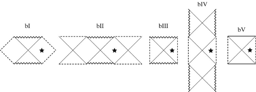
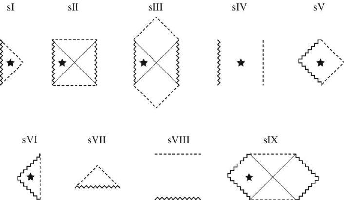
| type | type | type | ||||
| 1 | sI | sII | sIV | |||
| rI | rV | rVII | ||||
| bI | bII | bIII | ||||
| dsI | ||||||
| sVIII | ||||||
| 0 | sI | sII | sIV | |||
| — | rIV | rII | ||||
| sVII | sVIII | bIII | ||||
| -1 | sIII | sII | sIV | |||
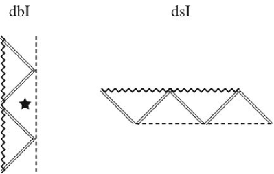
| rIII | rVI | dbI | ||||
| sVII | sVIII | bIV | ||||
| bV | ||||||
| bIII | ||||||
| , ( branch) | , ( branch) | , ( branch) | branch | |||||
| type | type | type | type | |||||
| 1 | sI | sII | sIV | sIV | ||||
| rI | rV | rVII | rVII | |||||
| bI | bII | bIII | ||||||
| dsI | ||||||||
| sVIII | ||||||||
| 0 | sI | sII | sIV | sIV | ||||
| — | rIV | rII | rII | |||||
| sVII | sVIII | bIII | ||||||
| -1 | sIII | sII | sIV | sIV | ||||
| sVII | sVIII | dbI | sIV | |||||
| sVII | sVIII | bIV | bIII | |||||
| rIII | rVI | bIII | bV | |||||
| bIII | bIV | |||||||
| bV | dbI | |||||||
| sIV | ||||||||
| ( branch) | ( branch) | ( branch) | branch | |||||
| type | type | type | type | |||||
| 1 | sI | sII | sIV | sIV | ||||
| rI | rV | rVII | rVII | |||||
| sV | sIX | sVI | ||||||
| bI | bII | bIII | ||||||
| dsI | ||||||||
| sVIII | ||||||||
| 0 | sI | sII | sIV | sIV | ||||
| — | rIV | rII | rII | |||||
| sVII | sVIII | bIII | ||||||
| -1 | sIII | sII | sIV | sIV | ||||
| sVII | sVIII | dbI | sIV | |||||
| sVII | sVIII | bIV | bIII | |||||
| rIII | rVI | bIII | bV | |||||
| bIII | sVI | |||||||
| bV | sIV | |||||||
| branch | branch | branch | branch | |||||
| type | type | type | type | |||||
| 1 | rVII | rVII | rVII | rVII | ||||
| bIII | sIV | sIV | sIV | |||||
| sVI | ||||||||
| bIII | ||||||||
| 0 | rII | rII | rII | rII | ||||
| bIII | sIV | bIII | sIV | |||||
| -1 | bV | bV | bV | bV | ||||
| bIII | bIV | bIII | bIII | |||||
| dbI | sVI | |||||||
| sIV | sIV | |||||||
References
-
(1)
N. Arkani-Hamed, S. Dimopoulos, and G. Dvali,
Phys. Lett. B 429, 263 (1998);
I. Antoniadis, N. Arkani-Hamed, S. Dimopoulos, and G. Dvali, Phys. Lett. B 436, 257 (1998). - (2) L. Randall and R. Sundrum, Phys. Rev. Lett. 83, 3370 (1999); 83, 4690 (1999).
-
(3)
G. Dvali, G. Gabadadze, and M. Porrati,
Phys. Lett. B 485, 208 (2000);
G. Dvali and G. Gabadadze, Phys. Rev. D 63, 065007 (2001);
G. Dvali, G. Gabadadze, and M. Shifman, Phys. Rev. D 67, 044020 (2003). -
(4)
P. Hořava and E. Witten,
Nucl. Phys. B475, 94 (1996);
A. Lukas, B. A. Ovrut, K.S. Stelle, and D. Waldram, Phys. Rev. D 59, 086001 (1999);
A. Lukas, B. A. Ovrut, and D. Waldram, Phys. Rev. D 60, 086001 (1999). -
(5)
S. Dimopoulos and G. Landsberg,
Phys. Rev. Lett. 87 (2001) 161602;
A. Chamblin and G.C. Nayak, Phys. Rev. D 66 (2002) 091901;
S. B. Giddings and S. Thomas, Phys. Rev. D 65 (2002) 056010. - (6) C. Lanczos, Ann. Math. 39, 842 (1938).
-
(7)
D. J. Gross and E. Witten,
Nucl. Phys. B277, 1 (1986);
D. J. Gross and J. H. Sloan, Nucl. Phys. B291, 41 (1987);
R. R. Metsaev and A. A. Tseytlin, Phys. Lett. B 191, 354 (1987);
R. C. Meyers, Phys. Rev. D 36, 392 (1987);
C. G. Callan, R. C. Meyers, and M. J. Perry, Nucl. Phys. B311, 673 (1988);
R. R. Metsaev and A. A. Tseytlin, Nucl. Phys. B293, 385 (1987). -
(8)
B. Zwieback,
Phys. Lett. B 156, 315 (1985);
B. Zumino, Phys. Rep. 137, 109 (1986). - (9) D. G. Boulware and S. Deser, Phys. Rev. Lett. 55, 2656 (1985).
- (10) J. T. Wheeler, Nucl. Phys. B268, 737 (1986).
- (11) See for example, T. Torii, H. Yajima, and K. Maeda, Phys. Rev. D 55, 739 (1997) and references therein.
- (12) Y.M. Cho and I. P. Neupane, Phys. Rev. D 66, 024044 (2002).
- (13) M. Cvetic, S. Nojiri, and S. D. Odintsov, Nucl. Phys. B628, 295 (2002).
- (14) R. -G. Cai, Phys. Rev. D 65, 084014 (2002).
- (15) I. P. Neupane, Phys. Rev. D 67, 061501(R) (2003); 69, 084011 (2004);
- (16) R. -G. Cai and Q. Guo, Phys. Rev. D 69, 104025 (2004).
- (17) J. D. Brown, J. Creighton, and R. B. Mann, Phys. Rev. Lett. 50, 6394 (1984).
- (18) See references in R. -G. Cai and K. -S. Soh, Phys. Rev. D 59, 044013 (1999).
- (19) D. Lovelock, J. Math. Phys. 12, 498 (1971).
- (20) R. C. Myers and J. Z. Simon, Phys. Rev. D 38, 2434 (1988).
- (21) B. Whitt, Phys. Rev. D 38, 3000 (1988).
- (22) S. Deser and B. Tekin, Phys. Rev. Lett. 89, 101101 (2002); Phys. Rev. D 67, 084009 (2003).
- (23) C. W. Misner, K.S. Thorne, and J.A. Wheeler, Gravitation, (Freeman, 1973).
- (24) J. A. Wolf, Space of Constant Curvature (MacGraw-Hill, New York, 1967).
- (25) S. Carlip, Class. Quantum Grav. 10, 207 (1993).
-
(26)
C. Böhm,
Invent. Math. 134, 145 (1998).
S. Carlip, Class. Quantum Grav. 15, 2629 (1998). - (27) For a rigorous definition, see S. W. Hawking, and G. F. R. Ellis, The large scale structure of space-time (Cambridge University Press, Cambridge, England, 1973).
- (28) When the -dimensional Einstein space is simply connected, the center is regular. When it is not, as with the topological black holes, the center becomes singular. This singularity is simply due to the topological structure of the Einstein space. Hence we use the word “regular” at the center, even in this case.
- (29) As we mentioned, in the higher-dimensional cases, the -dimensional Einstein space is not necessarily a sphere nor is its quotient space even for positive curvature. Hence the solution represents not only the (at least locally) Minkowski spacetime but also many others. However, here and in the following sections we refer to all of these together as “Minkowski spacetimes”.
- (30) V. Rychkov, Phys. Rev. D 70, 044003 (2004).
-
(31)
R. M. Wald,
Phys. Rev. D 48, R3427 (1993);
V. Iyer and R. M. Wald, Phys. Rev. D 50, 846 (1994). - (32) T. Clunan, S. F. Ross, and D. J. Smith, Class. Quantum Grav. 21, 3447 (2004).
- (33) C. Csaki, J. Erlich, and C. Grojean, Nucl. Phys. B604, 312 (2001).
-
(34)
R. Penrose,
in Battelle Rencontres, edited by C. de Witt, and J. A. Wheeler
(W.A. Benjamin, New York, 1968), p.222;
E. Poisson and W. Israel, Phys. Rev. D 41, 1796 (1990);
P. R. Brady, Prog. Theor. Phys. Suppl. 136, 29 (1999). - (35) See also the reference in H. Maeda, T. Torii, and T. Harada, Phys. Rev. D 71, 064015 (2005).
- (36) K. Maeda and T. Torii, Phys. Rev. D 69, 024002 (2004).
- (37) T. Torii (in preparation).