Abstract

We study the inflationary scenarios driven by a Wilson line field - the fifth component of a 5D gauge field and corresponding modulus field, within $S^{(1)}/Z_{2}$ orbifold supergravity (SUGRA). We use our off shell superfield formulation and give a detailed description of the issue of SUSY breaking by the $F$-component of the radion superfield. By a suitably gauged $U(1)_{R}$ symmetry and including couplings with compensator supermultiplets and a linear multiplet, we achieve a self consistent radion mediated SUSY breaking of no scale type. The inflaton 1-loop effective potential has attractive features needed for successful inflation. An interesting feature of both presented inflationary scenarios are the red tilted spectra with $n_{s}\simeq 0.96$. For gauge inflation we obtain a significant tensor to scalar ratio ($r\approx 0.1$) of the density perturbations, while for the modulus inflation $r$ is strongly suppressed.

1 Introduction

Inflation is the only candidate which naturally evades numerous cosmological problems [1]. In order to have a sufficiently flat universe, a de-Sitter type expansion with a slowly rolling scalar inflaton field is needed. This requires a flat inflaton potential and for that supersymmetry (SUSY) is believed to be crucial in a realistic model building [2]. A different possibility for realizing a flat potential is that the inflaton field is a pseudo Nambu-Goldstone Boson (PNGB) field [3]. However, this idea seems to be difficult to realize since it usually requires VEVs much higher than the Planck scale: at such large VEVs, one might not trust the results obtained in the framework of an (effective) quantum field theory (see a more detailed discussion in ref [4]). A nice and elegant realization of the PNGB inflation scenario was proposed in [4] (and subsequent works [5], [6]), where an extra dimensional construction was suggested and the PNGB inflaton is the Wilson line field corresponding to the fifth component of a 5D $U(1)$ gauge field. In this setting, the flatness of the inflaton potential does not require unnatural assumptions and the model turns out to be fully self consistent with an effective 4D quantum field theory setting. Although the idea of ref. [4] works without invoking SUSY, we think that (with its phenomenological and theoretical motivations) it is worthwhile to study this type of scenarios in the framework of SUSY. Our recent work [6] was dedicated to this issue and can be considered as a step towards the construction of the SUSY gauge inflation scenario. The setting which we have proposed there was based on a rigid on shell SUSY 5D construction of ref. [7] with the fifth dimension compactified on a circle $S^{(1)}$. The radion superfield $T$ was used for SUSY breaking by its auxiliary component $F_{T}\neq 0$.

The aim of the present paper is to extend studies to 5D orbifold supergravity (SUGRA). Our construction is based on the off shell formulation of 5D conformal SUGRA developed by Fujita, Kugo and Ohashi (FKO) [8], [9], [10] and uses the superfield approach suggested recently by us in ref. [11] (see also the subsequent ref. [12]). This superfield approach turned out to be very economical and powerful for studying various phenomenological and theoretical issues in 5D [15]. Here, we first present in section 2 the minimal setting which is needed in order to realize gauge inflation. Then in section 3 we give full account of the issue of SUSY breaking by the radion’s auxiliary $F$-component. We show that to obtain flatness and selfconsistency, gauging of a $U(1)_{R}$ part of the global $SU(2)_{R}$ symmetry and a linear multiplet with appropriate couplings with the $U(1)_{R}$ gauge supermultiplet play an important role. In section 4 we turn to the calculation of the one loop inflaton effective potential including the Wilson line and modulus fields. We separately study two inflationary scenarios: in section 5 the gauge inflation and in section 6 the inflation driven by the modulus field. We discuss features allowing to realize a natural inflation and give a detailed study of some properties for both inflationary scenarios.

2 The setting

In this letter we will deal with two types of hypermultiplets. One is a compensator (denoted by ${\bf h}$) and is necessary for gauge fixing of the conformal symmetry. The second type of hypermultiplet is a physical one- referred to as a matter hypermultiplet (denoted by ${\bf H}$). It will play an important role in the generation of the inflaton (the Wilson line field) potential. In general, 5D hypermultiplets ${\mathbb{H}}^{\alpha}=({\mathcal{A}}^{\alpha}_{i},~{}\zeta^{\alpha},{\cal F}^{\alpha}_{i})$ can be ordered into $r$ pairs $({\mathbb{H}}^{2\hat{\alpha}-1},~{}{\mathbb{H}}^{2\hat{\alpha}})$, where $\hat{\alpha}=1,2,\cdots,r$ (see [8]-[10] for a detailed discussion). In the following, we will use the notation

$${\bf H}\equiv({\bf H}_{1},~{}{\bf H}_{2})=(H,~{}H^{c})~{},$$ (1)

for such a pair (omitting the index $\hat{\alpha}$) and similar for the compensator ${\bf h}=({\bf h}_{1},{\bf h}_{2})=(h,h^{c})$. In the general discussion of the hypermultiplet case we will use ${\bf H}$ and understand that this similarly applies to the compensator. Essential differences for the compensator hypermultiplet, will be pointed out throughout the text. The 5D hypermultiplet of eq. (1) decomposes into a pair of ${\mathcal{N}}=1$ 4D chiral superfields with opposite orbifold parities [10]:

$$H=\left({\cal A}^{2\hat{\alpha}}_{2}=({\cal A}_{1}^{2\hat{\alpha}-1})^{*},~{}-2{\rm i}\zeta^{2\hat{\alpha}}_{R},~{}({\rm i}M_{*}{\cal A}+{\hat{{\mathcal{D}}}}_{5}{\cal A})^{2\hat{\alpha}}_{1}\right),$$

$$H^{c}=\left({\cal A}^{2\hat{\alpha}-1}_{2}=-({\cal A}^{2\hat{\alpha}}_{1})^{*},~{}-2{\rm i}\zeta^{2\hat{\alpha}-1}_{R},~{}({\rm i}M_{*}{\cal A}+{\hat{{\mathcal{D}}}}_{5}{\cal A})^{2\hat{\alpha}-1}_{1}\right),$$ (2)

with

$$M_{*}{\cal A}^{\alpha}_{i}=igM^{I}(t_{I})^{\alpha}_{\beta}{\cal A}^{\beta}_{i}+{\cal F}^{\alpha}_{i}~{},$$

$$\hat{{\mathcal{D}}}_{5}{\cal A}^{\alpha}_{i}=\partial_{5}{\cal A}^{\alpha}_{i}-igW_{5\beta}^{\alpha}{\cal A}^{\beta}_{i}-W_{5}^{0}\frac{1}{\alpha}{\cal F}^{\alpha}_{i}-\kappa V_{5ij}{\cal A}^{\alpha j}-2\kappa{\rm i}\bar{\psi}_{5i}\zeta^{\alpha}~{},$$ (3)

where $(t_{I})^{\alpha}_{\beta}$ is the generator of the gauge group $G_{I}$. In this paper we will deal only with abelian gauge groups. In this case the gauge coupling $g$ should be replaced by $g/2$. The components $(\phi,\psi,F_{\Phi})$ of a 4D chiral superfield $\Phi$ are assumed to be of ’right handed’ chirality. Therefore, the superfield with a left chirality in a two component notation is given by

$$\Phi=(\phi,\psi,F_{\phi})=\phi^{*}+\theta\psi_{L}-\theta^{2}F_{\Phi}^{*}~{}.$$ (4)

We will use this basis during the calculations.

Besides the hypermultiplets, in this discussion, three 5D gauge supermultiplets $(V,\Sigma)^{I}$ will be considered. i) The $U(1)_{Z}$ central charge symmetry corresponds to $I=0$: $(V,\Sigma)^{I=0}\equiv(V_{0},\Sigma_{0})$. This is a compensating gauge supermultiplet and, as was observed in [11], in the rigid limit accounts for the radion superfield. In the covariant derivatives of eq. (3) $I=0$ does not participate in $M^{I}(t_{I})^{\alpha}_{\beta}$ and $W^{\alpha}_{5\beta}$, but acts only on an auxiliary component ${\cal F}^{\alpha}_{i}$. This is a particular property of the compensating $I=0$ gauge supermultiplet. ii) Our construction is based on a gauged $U(1)_{R}$ symmetry whose corresponding gauge supermultiplet is $(V,\Sigma)^{I=R}\equiv(V_{R},\Sigma_{R})$. Only the compensator hypermultiplet ${\bf h}$ is charged under this group. iii) Finally, we introduce an $U(1)$ gauge supermultiplet $(V,\Sigma)^{I=1}\equiv(V_{1},\Sigma_{1})$, where $\Sigma_{1}$ contains the fifth component of a vector field which generates the Wilson line field $\Theta=\int dyA_{5}$. The latter being a 4D scalar will play the role of the inflaton field in the following. Note that only the matter hypermultiplet ${\bf H}$ is charged under $(V_{1},\Sigma_{1})$.

The orbifold $Z_{2}$ parities ($y\to-y$) of the introduced gauge supermultiplets are given as:

$$Z_{2}:~{}~{}~{}(V_{0},V_{R},V_{1})\to-(V_{0},V_{R},V_{1})~{},~{}~{}~{}~{}~{}(\Sigma_{0},\Sigma_{R},\Sigma_{1})\to(\Sigma_{0},\Sigma_{R},\Sigma_{1})~{}.$$ (5)

Therefore all 4D gauged $U(1)$ symmetries are broken on the orbifold fixed points. As far as the hypermultiplets are concerned, without loss of generality we can consider the following orbifold parity prescriptions:

$$Z_{2}:~{}~{}~{}H\to H~{},~{}~{}~{}~{}~{}H^{c}\to-H^{c}~{}.$$ (6)

For all gauge fields $(V_{I},\Sigma_{I})$ we introduce the following parameterization

$${\bf V}^{ab}=gV\vec{q}\cdot\vec{\sigma}^{a}_{b}~{},~{}~{}~{}~{}{\bf\Sigma}^{ab}=g\Sigma\vec{q}\cdot\vec{\sigma}^{a}_{b}~{},~{}~{}~{}{\rm with}~{}~{}~{}|\vec{q}|=1~{}.$$ (7)

With this, the hypermultiplet Lagrangian is given by [15]

$$e_{(4)}^{-1}{\cal L}({\rm hyper})=\int d^{4}\theta{\mathbb{W}}_{y}2{\bf H}_{a}^{\dagger}(e^{-2{\bf V}})^{ab}{\bf H}_{b}-\int d^{2}\theta({\bf H}\epsilon)_{a}(\hat{\partial}_{y}-{\bf\Sigma})^{ab}{\bf H}_{b}+{\rm h.c.}~{}$$ (8)

In case of the compensator, the Lagrangian eq.(8) should come with opposite sign. The superoperator $\hat{\partial}_{y}$ is obtained by promoting ${\partial}_{y}$ to an operator containing odd (under orbifold parity) elements of the 5D Weyl multiplet (see [11] for a more detailed discussion), which do not have any relevance for our purposes and can be ignored.

With the orbifold parity assignments given in (5) and (6) we should gauge the $U(1)$ symmetries of (7) in $\sigma^{1},\sigma^{2}$ direction, i.e. $q_{3}=0$ . In (8) ${\mathbb{W}}_{y}$ is a real general type 4D supermultiplet which contains part of the radion chiral superfield as [11]

$${\mathbb{W}}_{y}=\frac{1}{2}(T+T^{\dagger})+\cdots$$ (9)

This relation is useful to account for the radion coupling with hypermultiplets. Since all 4D gauge superfields $V$ have negative orbifold parities in this setting, they do not contain zero mode states and will be irrelevant for us. Therefore, we will set further $V=0$. Taking all this into account, the action (8) for matter and compensator hypermultiplets can be written as:

$${\cal L}({\rm hyper})|_{V=0}={\cal L}(H)+{\cal L}(h)~{},$$

$$e_{(4)}^{-1}{\cal L}(H)=\int d^{4}\theta(T+T^{\dagger})\left(H^{\dagger}H+H^{c\dagger}H^{c}\right)+\int d^{2}\theta\left(2H^{c}\partial_{y}H+g_{1}\Sigma_{1}(e^{{\rm i}\hat{\theta}_{1}}H^{2}-e^{-{\rm i}\hat{\theta}_{1}}H^{c2})\right)+{\rm h.c.}$$

$$e_{(4)}^{-1}{\cal L}(h)=-\int d^{4}\theta(T+T^{\dagger})\left(h^{\dagger}h+h^{c\dagger}h^{c}\right)-\int d^{2}\theta\left(2h^{c}\partial_{y}h+g_{R}\Sigma_{R}(e^{{\rm i}\hat{\theta}_{R}}h^{2}-e^{-{\rm i}\hat{\theta}_{R}}h^{c2})\right)+{\rm h.c.}$$ (10)

where $\cos\hat{\theta}_{1}=q_{1}^{1}$, $\sin\hat{\theta}_{1}=q_{2}^{1}$, $\cos\hat{\theta}_{R}=q_{1}^{R}$, $\sin\hat{\theta}_{R}=q_{2}^{R}$.

3 SUSY breaking through the radion superfield

In our model, for SUSY breaking we will use a non-zero $F$ component of the radion superfield $T$. As it was pointed out in ref.[11], to obtain a flat tree-level potential for $F_{T}$ we need to introduce a linear multiplet ${\bf L}$ which couples with the $V^{I=R}$ vector multiplet. As we will see below, the rôle of ${\bf L}$ is to insure a self consistent SUSY breaking. Assuming that ${\bf L}$ is neutral under $V^{I=R}$, its field content is [9]

$${\bf L}=(L^{ij}~{},\phi^{i}~{},E^{\mu\nu}~{},N)~{},$$ (11)

where $E^{\mu\nu}$ is an unconstrained antisymmetric tensor field. The coupling action of ${\bf L}-V^{I=R}$ is given by

$$e^{-1}{\cal L}(V^{I=R},{\bf L})=Y_{R}^{ij}L_{ij}+2\overline{\Omega}_{R}^{i}\phi_{i}+2{\rm i}\overline{\psi}_{i}^{a}\gamma_{a}\Omega_{Rj}L^{ij}+$$

$$\frac{1}{2}M_{R}\left(N-2{\rm i}\overline{\psi}_{b}\gamma^{b}\phi-2{\rm i}\overline{\psi}_{a}^{i}\gamma^{ab}\psi^{j}_{b}L_{ij}\right)+\frac{1}{4}e^{-1}F_{\mu\nu}(W_{R})E^{\mu\nu}~{}.$$ (12)

${\bf L}$ plays the role of a Lagrange multiplier. A variation with respect to the components of ${\bf L}$ leads to

$$M_{R}=0~{},~{}~{}~{}~{}\overline{\Omega}_{R}^{i}=0~{},~{}~{}~{}~{}Y_{R}^{ij}=0~{},~{}~{}~{}~{}F_{\mu\nu}(W_{R})=0~{}.$$ (13)

The last equation of (13) has the solution

$$W_{5R}={\rm constant}~{}.$$ (14)

This is enough to insure a non zero $F$ component of $T$.

Consider the part of the action (10) which involves the compensator hypermultiplet. The relevant bosonic couplings have the form

$$e_{(4)}^{-1}{\cal L}(h)\supset-2\left|F_{h}+\partial_{5}h^{c*}-g_{R}\Sigma_{R}^{*}e^{{\rm i}\hat{\theta}_{R}}h^{*}+\frac{1}{2}F_{T}h\right|^{2}+2\left|\partial_{5}h^{c*}-g_{R}\Sigma_{R}^{*}e^{{\rm i}\hat{\theta}_{R}}h^{*}+\frac{1}{2}F_{T}h\right|^{2}-$$

$$2\left|F_{h^{c}}-\partial_{5}h^{*}+g_{R}\Sigma_{R}^{*}e^{-{\rm i}\hat{\theta}_{R}}h^{c*}+\frac{1}{2}F_{T}h^{c}\right|^{2}+2\left|\partial_{5}h^{*}-g_{R}\Sigma_{R}^{*}e^{-{\rm i}\hat{\theta}_{R}}h^{c*}-\frac{1}{2}F_{T}h^{c}\right|^{2}+$$

$$g_{R}F_{\Sigma_{R}}^{*}\left(e^{{\rm i}\hat{\theta}_{R}}(h^{*})^{2}-e^{-{\rm i}\hat{\theta}_{R}}(h^{c*})^{2}\right)+{\rm h.c.}$$ (15)

where for the lowest components of the hypermultiplet we have used the same notation as for the corresponding superfield. From (2), (3) we have

$$F_{h}={\cal F}_{h}-\partial_{5}h^{c*}-{\rm i}\frac{g_{R}}{2}W_{5R}e^{{\rm i}\hat{\theta}_{R}}h^{*}+\frac{1}{2}F_{T}h~{},$$

$$F_{h^{c}}={\cal F}_{h^{c}}+\partial_{5}h^{*}+{\rm i}\frac{g_{R}}{2}W_{5R}e^{-{\rm i}\hat{\theta}_{R}}h^{c*}+\frac{1}{2}F_{T}h^{c}~{},~{}~{}{\rm with}~{}~{}{\cal F}_{h}=({\rm i}-\frac{W_{5}^{0}}{\alpha}){\cal F}^{2\hat{\alpha}}_{h1}~{},~{}~{}{\cal F}_{h^{c}}=({\rm i}-\frac{W_{5}^{0}}{\alpha}){\cal F}^{2\hat{\alpha}-1}_{h1}~{},$$ (16)

where the relations

$$\Sigma_{R}=-\frac{\rm i}{2}W_{5R}~{},~{}~{}~{}~{}\kappa(V_{5}^{1}+{\rm i}V_{5}^{2})=-\frac{{\rm i}F_{T}}{e_{y}^{5}}~{},~{}~{}~{}{\rm with}~{}~{}~{}e_{y}^{5}=1$$ (17)

have been used. Taking into account all this and the constraints $h=\kappa^{-1},h^{c}=0$, (15) reduces to

$$e_{(4)}^{-1}{\cal L}(h)\supset-2\left|{\cal F}_{h}-{\rm i}g_{R}W_{5R}e^{{\rm i}\hat{\theta}_{R}}\kappa^{-1}+F_{T}\kappa^{-1}\right|^{2}-2\left|{\cal F}_{h^{c}}\right|^{2}+$$

$$\frac{\kappa^{-2}}{2}\left|F_{T}-{\rm i}g_{R}W_{5R}e^{{\rm i}\hat{\theta}_{R}}\right|^{2}+g_{R}\kappa^{-2}(F_{\Sigma_{R}}e^{-{\rm i}\hat{\theta}_{R}}+{\rm h.c.})~{}.$$ (18)

The on-shell equations $\frac{\partial{\cal L}}{\partial{\cal F}_{h}}=\frac{\partial{\cal L}}{\partial{\cal F}_{h^{c}}}=\frac{\partial{\cal L}}{\partial F_{T}}=0$ then have the solutions

$$F_{T}={\rm i}g_{R}W_{5R}e^{{\rm i}\hat{\theta}_{R}}~{},~{}~{}~{}~{}{\cal F}_{h}={\cal F}_{h^{c}}=0~{}.$$ (19)

Therefore, gauging $U(1)_{R}$ we have obtained a non zero $F_{T}$ with a flat potential. This is a no-scale SUSY breaking scenario with SUSY breaking mediated by the radion superfield. For a discussion of this phenomenon within a 5D on shell construction see [16], [17]. An $F_{T}\neq 0$ is important for transmitting the SUSY breaking into the matter sector. All states which carry an $SU(2)_{R}$ index, couple with $F_{T}$ through the covariant derivative and obtain a soft SUSY breaking mass. For instance, the zero mode of the 4D gravitino obtains a soft mass through the 5D gravitino kinetic term by mixing with $\psi_{5-}\equiv{\rm i}(\psi_{5L}^{1}+\psi_{5R}^{2})$. The latter is a goldstino - the fermionic component of the radion superfield.

Concluding this section, let us comment on another role of the linear multiplet. It insures that all other $F$-terms are zero. The first term of (12) can be written as

$$Y_{R}^{ij}L_{ij}=2Y_{R}^{a}L^{a}=(F_{\Sigma_{R}}L+{\rm h.c.})+\cdots~{},$$ (20)

where $L=-L^{1}+{\rm i}L^{2}$ and ellipses stand for terms which are irrelevant for us. Collecting together all couplings containing $F_{\Sigma_{R}}$, we have

$$e_{(4)}^{-1}{\cal L}(F_{\Sigma_{R}})=2\left|F_{\Sigma_{R}}\right|^{2}+F_{\Sigma_{R}}(g_{R}\kappa^{-2}e^{-{\rm i}\hat{\theta}_{R}}+L)+{\rm h.c.}$$ (21)

The conditions $\frac{\partial{\cal L}}{\partial F_{\Sigma_{R}}}=\frac{\partial{\cal L}}{\partial L}=0$ are satisfied by the solutions

$$F_{\Sigma_{R}}=0~{},~{}~{}~{}~{}~{}L=-g_{R}\kappa^{-2}e^{-{\rm i}\hat{\theta}_{R}}~{}.$$ (22)

Note, that without the coupling to the lowest component of the linear multiplet, we would not be able to have $F_{\Sigma_{R}}=0$. The latter is needed for the $F$-flatness and a vanishing vacuum energy on the classical level.

Together with the gauge inflation, below we will also study the inflation driven by the modulus field $M^{1}$. With $\langle M^{1}\rangle\neq 0$ the corresponding $F_{\Sigma_{1}}$ will have the potential: $\int de^{4}\theta 2{\mathbb{W}}_{y}P({\cal V}_{5})\to-{\cal N}_{11}|F_{\Sigma_{1}}-\frac{1}{2}M^{1}F_{T}|^{2}$. This gives

$$F_{\Sigma_{1}}=\frac{1}{2}M^{1}F_{T}~{},$$ (23)

which will play an important role for calculation of the masses of KK states.

4 KK decomposition and inflaton potential

Now we are ready to derive the inflation effective potential. Relevant for us is the 4D chiral superfield $\Sigma_{1}$ which contains the fifth component $A_{5}^{1}$ of $U(1)$ and the corresponding (real) modulus $M^{1}$ as $\Sigma_{1}=\frac{1}{2}(M^{1}-{\rm i}A_{5}^{1})$. The superfield $\Sigma_{1}$ has positive $Z_{2}$ orbifold parity and therefore the Wilson line field

$$\Theta=\int dyA_{5}=2\pi RA_{5}^{1}~{},$$ (24)

and (the zero mode of) $M^{1}$ are $y$-independent 4D scalars. Taking all this into account, from (10) with (23) one can easily derive the potential for the scalar components $H,H^{c}$ with phase redefinition $H\to e^{{\rm i}\hat{\theta}_{1}/2}H$, $H^{c}\to e^{-{\rm i}\hat{\theta}_{1}/2}H^{c}$:

$$V(H)=2\left|\partial_{5}H-\frac{g_{1}}{2}(M^{1}-\frac{{\rm i}\Theta}{2\pi R})H^{c}-\frac{1}{2}F_{T}^{*}H^{c*}\right|^{2}+2\left|\partial_{5}H^{c}-\frac{g_{1}}{2}(M^{1}-\frac{{\rm i}\Theta}{2\pi R})H+\frac{1}{2}F_{T}^{*}H^{*}\right|^{2}+$$

$$\frac{1}{2}g_{1}M^{1}F_{T}(H^{2}-H^{c2})+\frac{1}{2}g_{1}M^{1}F_{T}^{*}(H^{*2}-H^{c*2})~{}.$$ (25)

With the parity assignment (6), the KK decomposition for $H$, $H^{c}$ is given by

$$H=\frac{1}{2\sqrt{\pi R}}H^{(0)}+\frac{1}{\sqrt{2\pi R}}\sum_{n\neq 1}H^{(n)}\cos\frac{ny}{R}~{},~{}~{}~{}~{}~{}H^{c}=\frac{1}{\sqrt{2\pi R}}\sum_{n\neq 1}\overline{H}^{\hskip 1.70717pt(n)}\sin\frac{ny}{R}~{}.$$ (26)

Upon integration along the fifth dimension ${\cal L}^{(4)}=\int_{0}^{2\pi R}dy{\cal L}^{(5)}$, one can easily see that the mass² of the two real zero modes are

$$(m_{\pm}^{(0)})^{2}=\frac{1}{R^{2}}(\frac{g_{1}\Theta}{4\pi}\pm\frac{1}{2}R|F_{T}|)^{2}~{}.$$ (27)

For KK states it is convenient to choose the basis $H^{(n)}=\frac{\rm i}{\sqrt{2}}(H^{(n)}_{-}-H^{(n)}_{+})$, $\overline{H}^{(n)}=\frac{1}{\sqrt{2}}(H^{(n)}_{-}+H^{(n)}_{+})$. The mass² matrices for appropriate $n$-th KK modes are

$$\begin{array}[]{cc}&{\begin{array}[]{cc}H^{(n)}_{-}&\hskip 85.35826ptH^{\hskip 1.70717pt(n)*}_{-}\end{array}}\\ \vspace{5mm}\begin{array}[]{c}H^{(n)*}_{-}\\ H^{\hskip 1.70717pt(n)}_{-}\end{array}\!\!\!\!\!&{\left(\begin{array}[]{cccc}(n+\frac{g_{1}\Theta}{4\pi})^{2}+\frac{1}{4}|RF_{T}|^{2}+\frac{1}{4}(g_{1}RM^{1})^{2}&{\rm i}(n+\frac{g_{1}\Theta}{4\pi})RF_{T}^{*}\vspace{0.2cm}\\ -{\rm i}(n+\frac{g_{1}\Theta}{4\pi})RF_{T}^{*}&(n+\frac{g_{1}\Theta}{4\pi})^{2}+\frac{1}{4}|RF_{T}|^{2}+\frac{1}{4}(g_{1}RM^{1})^{2}\end{array}\right)\frac{1}{2R^{2}}}~{},\end{array}\!\!$$ (28)

and similar for $H^{\hskip 1.70717pt(n)}_{+}$ states. For mass²’s of four real scalar states (per $n\neq 0$ KK state) we thus get

$$[m^{(n)}(H_{-})]^{2}_{\pm}=[m^{(n)}(H_{+})]^{2}_{\pm}=\frac{1}{R^{2}}(n+\frac{g_{1}\Theta}{4\pi}\pm\frac{1}{2}|RF_{T}|)^{2}+\frac{1}{2}(g_{1}M^{1})^{2}~{}.$$ (29)

A non-zero $F_{T}$ does not affect the masses of the fermionic components ($\psi_{H}$, $\overline{\psi}_{H^{c}}$) coming from $H_{M},H_{M}^{c}$ because they are blind with respect of $SU(2)_{R}$. Therefore the masses of Majorana fermionic components are

$$m^{(n)}(\psi_{H})=\frac{1}{R}(n-g_{1}\frac{\Theta}{4\pi})~{},~{}~{}~{}~{}n=-\infty,\cdots,\infty~{},$$

$$m^{(n)}(\overline{\psi}_{H^{c}})=\frac{1}{R}(n+g_{1}\frac{\Theta}{4\pi})~{},~{}~{}~{}~{}n=-\infty,\cdots,\infty~{},~{}~{}~{}n\neq 1~{}.$$ (30)

Note that the spectrum in (29), (30) is equivalent to one obtained within the Scherck-Schwarz SUSY breaking scenario.

As we have already mentioned, integration of the states with $\Theta$-dependent masses induces an effective 1-loop potential for $\Theta$. The potential will also depend on the modulus $M^{1}$. Using Poisson resummation for each KK mode’s contribution to the effective potential (or starting from a worldline expression, see an appendix in [6]), we finally obtain

$${\cal V}^{\rm eff}(\phi_{\Theta})=\frac{3}{16\pi^{6}R^{4}}\sum_{k=1}^{\infty}\frac{1}{k^{5}}\left(1-\cos(\pi kR|F_{T}|)\right)\cdot\cos(\pi kg_{4}R\phi_{\Theta})\times$$

$$e^{-\pi kg_{4}R|\phi_{M}|}\left(1+\pi kg_{4}R|\phi_{M}|+\frac{1}{3}(\pi kg_{4}R|\phi_{M}|)^{2}\right)~{}.$$ (31)

The effective potential in (31) is written in terms of canonically normalized 4D scalar fields $\phi_{\Theta}=\Theta/\sqrt{2\pi R}$, $\phi_{M}=\sqrt{2\pi R}M^{1}$ and dimensionless 4D gauge coupling $g_{4}=g_{1}/\sqrt{2\pi R}$ (for a general cubic norm function the field $\phi_{M}$ is canonically normalized in the global minimum with $\langle\phi_{M}\rangle=0$).

Notice that the divergent bosonic and fermionic contributions at $k=0$ cancel exactly because of SUSY. In the limit $F_{T}\to 0$ (unbroken SUSY) the effective one-loop potential vanishes. The potential in (31) is invariant under the shifts $\phi_{\Theta}\to\phi_{\Theta}+\frac{2k_{1}}{kg_{4}R}$, $|F_{T}|\to|F_{T}|+\frac{2k_{2}}{kR}$ ($k_{1,2}=$integer) reflecting the invariance under 5D gauge symmetries. Besides the $\phi_{\Theta}$ ($\phi_{M}$)-dependent part, the potential gets a constant contribution by integration of states which are neutral under $(V_{1},\Sigma_{1})$ but feel SUSY breaking through $F_{T}$. These kind of states are for example the 4D gravitino, the gauginos and $(V_{1},\Sigma_{1})$ neutral bulk hypermultiplets. Thus we add a constant part to the potential in eq. (31) and tune the former in such a way that the potential is zero in the global minimum (this is the usual fine tuning of the 4D cosmological constant). Keeping the dominant terms of (31), the inflaton potential will have the form

$${\cal V}={\cal V}^{\rm eff}\left.\right|_{k=1}+{\cal V}_{0}~{},~{}~{}~{}~{}{\rm with}~{}~{}~{}~{}{\cal V}_{0}=\frac{3}{16\pi^{6}R^{4}}\left(1-\cos(\pi R|F_{T}|)\right)~{}.$$ (32)

It’s profile is plotted in Fig. 1. For $F_{T}\not=0$ and $g_{4}R\phi_{\Theta}\neq 1$, $\phi_{M}\neq 0$ the potential ${\cal V}$ is positive, and thus it drives de Sitter expansion. Since ${\cal V}$ depends on two dynamical fields we will have inflation driven by these two fields. Below we will study the two extreme cases where one of the fields lies in its minimum and the inflation is driven by only one field. This allows an analytical study of the inflation and spectral properties of the density perturbations. The analysis for two field inflation will be presented elsewhere.

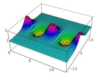
Figure 1: Effective potential as a function of $X=\pi g_{4}R\phi_{M}$ and $Y=\pi g_{4}R\phi_{\Theta}$.

5 Gauge inflation

First we consider the inflation driven by $\phi_{\Theta}$ and set $\phi_{M}=0$. In this case the two ’slow roll’ parameters are

$$\epsilon=\frac{(M_{\rm Pl})^{2}}{2}\left(\frac{{\cal V}^{\prime}}{{\cal V}}\right)^{2}=\frac{\pi^{2}}{2}(g_{4}RM_{\rm Pl})^{2}\tan^{2}\frac{\pi g_{4}R\phi_{\Theta}}{2}~{},$$

$$|\eta|=(M_{\rm Pl})^{2}\left|\frac{{\cal V}^{\prime\prime}}{{\cal V}}\right|=\frac{\pi^{2}}{2}(g_{4}RM_{\rm Pl})^{2}|\tan^{2}\frac{\pi g_{4}R\phi_{\Theta}}{2}-1|~{}.$$ (33)

[${\cal V}^{\prime}$, ${\cal V}^{\prime\prime}$ denote derivatives with respect to $\phi_{\Theta}$, and $M_{\rm Pl}=2.4\cdot 10^{18}$ GeV]. For moderate values of $\tan^{2}\frac{\pi g_{4}R\phi_{\Theta}}{2}$ the slow roll conditions $\epsilon,|\eta|\ll 1$ can be easily satisfied by properly suppressed $g_{4}$. Therefore, this is a good framework for a natural inflation. The value $\phi_{\Theta}^{f}$ at which the inflation ends is determined from the conditions $\epsilon,|\eta|\sim 1$

$$\tan\frac{\pi g_{4}R\phi_{\Theta}^{f}}{2}\simeq\frac{\sqrt{2}}{\pi g_{4}RM_{\rm Pl}}~{},$$ (34)

(we are considering the interval $0\leq g_{4}R\phi_{\Theta}\leq 1$). The fulfillment of the slow roll conditions allows to determine analytically the number of ${\rm e}$-foldings during the corresponding time interval

$$N(\phi_{\Theta}\to\phi_{\Theta}^{f})=\frac{1}{M_{\rm Pl}^{2}}\hskip 2.84544pt\int_{\phi_{\Theta}^{f}}^{\phi_{\Theta}}\frac{{\cal V}}{{\cal V}^{\prime}}d\phi_{\Theta}=-\frac{1}{(\pi g_{4}RM_{\rm Pl})^{2}}\ln\left(\sin^{2}\frac{\pi g_{4}R\phi_{\Theta}}{2}[1+\frac{1}{2}(\pi g_{4}RM_{\rm Pl})^{2}]\right)~{}.$$ (35)

With this expression one can calculate the value $\phi_{\Theta}^{Q}$ which corresponds to the epoch when the present horizon scale crossed outside the inflationary horizon scale. From the present observations we have $N_{Q}=55-60$ and therefore we need $\pi g_{4}RM_{\rm Pl}\ll 1$. We will use the latter relation for approximating the exact expressions. Using (35) we get

$$\phi_{\Theta}^{Q}\simeq\frac{2}{\pi g_{4}R}\arcsin\left(\exp[-\frac{N_{Q}}{2}(\pi g_{4}RM_{\rm Pl})^{2}]\right)\approx\frac{0.79}{g_{4}R}~{}~{}~{}{\rm with}~{}~{}N_{Q}=60~{},RM_{\rm Pl}=10~{},g_{4}=1.4\cdot 10^{-3}.$$ (36)

We see that for this value $\tan^{2}\frac{\pi g_{4}R\phi_{\Theta}}{2}$ is not small. The slow roll parameters

$$\epsilon_{Q}\simeq\frac{1}{2N_{Q}}~{},~{}~{}~{}~{}\eta_{Q}\simeq\frac{1}{2N_{Q}}-\frac{\pi^{2}}{2}(g_{4}RM_{\rm Pl})^{2}$$ (37)

however are small enough and we therefore have the relation $3H\dot{\phi}_{\Theta}=-{\cal V}^{\prime}$.

The quadrupole anisotropy of the temperature fluctuations due to the scalar perturbations can be calculated according to expression[20]

$$\left(\frac{\delta T}{T}\right)_{Q-S}=\left.\frac{\sqrt{5}}{60\pi}\frac{{\cal V}^{3/2}}{M_{\rm Pl}^{3}{\cal V}^{\prime}}\right|_{\phi_{\Theta}^{Q}}~{},$$ (38)

and for our case is given by

$$\left(\frac{\delta T}{T}\right)_{Q-S}=-\frac{1}{3\pi^{2}\sqrt{10}}\frac{1}{g_{4}RM_{\rm Pl}}\left(\frac{{\cal V}_{0}}{M_{\rm Pl}^{4}}\right)^{1/2}\sinh\left(-\frac{N_{Q}}{2}(\pi g_{4}RM_{\rm Pl})^{2}\right)\sim\frac{N_{Q}}{8\sqrt{30}\pi^{3}}\frac{g_{4}}{RM_{\rm Pl}}~{},$$ (39)

while the tensor to scalar ratio $r=\left(\frac{\delta T}{T}\right)_{Q-T}^{2}/\left(\frac{\delta T}{T}\right)_{Q-S}^{2}\simeq 2.16\pi\left(\frac{M_{\rm Pl}{\cal V}^{\prime}}{\cal V}\right)^{2}$ is

$$r\simeq 4.32\pi\epsilon_{Q}\simeq\frac{6.8}{N_{Q}}~{}.$$ (40)

From (39), (40) with $N_{Q}=60$, $g_{4}=1.4\cdot 10^{-3}$, $RM_{\rm Pl}=10$ one obtains the measured value $\left(\frac{\delta T}{T}\right)_{Q}\sim 6\cdot 10^{-6}$. For the same values of the parameters one has relatively large $r\simeq 0.11$. This is one of the remarkable feature of this inflationary scenario. The planned measurements of the Planck satellite could detect such a value of the tensor contribution. It is interesting to note that a quadratic inflaton potential gives a similar relation ($r\simeq 6.8/N_{Q}$.), although the scenario considered there differs from ours in various aspects. The spectral index $n_{s}=1+2\eta_{Q}-6\epsilon_{Q}$ for the scenario considered here is

$$n_{s}=1-\frac{2}{N_{Q}}-\pi^{2}(g_{4}RM_{\rm Pl})^{2}~{}.$$ (41)

We see that the spectrum is red-tilted. For parameters given in (36) we have $n_{s}\simeq 0.96$, which is compatible with WMAP data [21]. Combining WMAP and the Ly$\alpha$ data [22] gives the restriction $n_{s}\stackrel{{\scriptstyle>}}{{{}_{\sim}}}0.96$. In Table 1 we present the results for several cases satisfying this data.

Table 1: Spectral properties from gauge inflation with different values of parameters and $\left(\frac{\delta T}{T}\right)_{Q}\sim 6\times 10^{-6}$.

$$\begin{array}[]{|c|c|c|c|c|c|}\hline\cr N_{Q}&RM_{\rm Pl}&g_{4}&n_{s}&r&10^{3}\times\frac{dn_{s}}{d\ln k}\\ \hline\cr\hline\cr 55&5&7.4\cdot 10^{-4}&0.96&0.12&-0.67\\ \hline\cr 55&10&1.5\cdot 10^{-3}&0.96&0.12&-0.78\\ \hline\cr\hline\cr 60&5&7\cdot 10^{-4}&0.97&0.11&-0.56\\ \hline\cr 60&10&1.4\cdot 10^{-3}&0.96&0.11&-0.65\\ \hline\cr\end{array}$$

As we see the tensor to scalar ratio $r$ is significant while the spectral index practically shows no running. One can check that for presented cases $\phi_{\Theta}^{Q}>M_{\rm Pl}$. However, since $\phi_{\Theta}$ corresponds to the gauge field $A_{5}^{1}$ one can be sure that 5D gauge invariance and locality will guarantee that there is no undesirable corrections to the inflaton potential. The non local operators, not respecting the shift symmetry $\phi_{\Theta}\to\phi_{\Theta}+\frac{2k}{g_{4}R}$, are suppressed by a factor $e^{-2\pi RM_{5}}$ [4], where $M_{5}$ is the 5D Planck scale. For $R\stackrel{{\scriptstyle>}}{{{}_{\sim}}}\frac{5}{M_{5}}$ the suppression factor is $e^{-2\pi RM_{5}}\stackrel{{\scriptstyle<}}{{{}_{\sim}}}10^{-13}$. Therefore, all kind of non local contributions can be safely ignored.

6 Modulus field driven inflation

Now we consider the case in which the inflation is only due to modulus field $\phi_{M}$, assuming that $\phi_{\Theta}$ is settled in its minimum $g_{4}R\phi_{\Theta}=1$. For simplicity we will consider the norm function $\kappa^{-1}{\cal N}=(M^{0})^{3}-M^{0}(M^{1})^{2}$. Using the constraint ${\cal N}=\kappa^{-2}$, the field $\phi_{M}$ is not canonically normalized when $\langle\phi_{M}\rangle\neq 0$. For parameterisation of the very special manifold we introduce a new variable $t$ such that

$$M^{0}=\kappa^{-1}\cosh^{2/3}\alpha t~{},~{}~{}~{}M^{1}=\frac{\phi_{M}}{\sqrt{2\pi R}}=\kappa^{-1}\frac{\sinh\alpha t}{\cosh^{1/3}\alpha t}~{},~{}~{}~{}{\rm with}~{}~{}~{}\alpha=\frac{\kappa}{\sqrt{2\pi R}}=\frac{1}{M_{\rm Pl}}~{}.$$ (42)

Then the kinetic term has the form

$$\frac{1}{2}g(t)(\partial_{\mu}t)^{2}=\frac{1}{2}(\partial_{\mu}F)^{2}~{},~{}~{}~{}{\rm with}~{}~{}~{}\sqrt{g(t)}dt=dF~{},~{}~{}g(t)=1+\frac{1}{3}\tanh^{2}\alpha t~{},$$ (43)

where $F$ is a canonically normalized field playing the role of the modulus inflaton. Using the dimensionless variables

$$\phi_{R}=R\phi_{M}~{},~{}~{}~{}~{}t_{P}=\frac{1}{M_{\rm Pl}}t~{},$$ (44)

the derivatives can be written as

$$\frac{d{\cal V}}{dF}=\frac{1}{M_{\rm Pl}}\frac{1}{\sqrt{g}}\frac{\partial{\cal V}}{\partial\phi_{R}}\frac{\partial\phi_{R}}{\partial t_{P}}~{},$$

$$\frac{d^{2}{\cal V}}{dF^{2}}=\frac{1}{M_{\rm Pl}^{2}}\frac{1}{g}\left(\frac{\partial^{2}{\cal V}}{\partial\phi_{R}^{2}}\left(\frac{\partial\phi_{R}}{\partial t_{P}}\right)^{2}+\frac{\partial{\cal V}}{\partial\phi_{R}}\left(\frac{\partial^{2}\phi_{R}}{\partial t_{P}^{2}}-\frac{1}{2g}\frac{\partial\phi_{R}}{\partial t_{P}}\frac{\partial g}{\partial t_{P}}\right)\right)~{}.$$ (45)

Using these relations we can calculate the slow roll parameters $\epsilon$, $\eta$ which allows to determine numerically the point $t_{P}^{f}$ corresponding to the end of inflation. The $t_{P}^{Q}$ can be determined through the number of e-foldings through the relation

$$N_{Q}=\int_{t_{P}^{f}}^{t_{P}^{Q}}\sqrt{\frac{g(t_{P})}{2\epsilon(t_{P})}}dt_{P}~{}.$$ (46)

Having determined $t_{P}^{Q}$ we can calculate the quantities $\delta T/T$, $n_{s}$ and $r$. The selection of $g_{4},R$ should be done in such a way as to have $\frac{\delta T}{T}\approx 6\cdot 10^{-6}$. Numerical study shows that one can have inflation both for large and small values of $a\equiv\pi g_{4}RM_{Pl}$. For $a\gg 1$ we have

$$\pi g_{4}R\phi_{M}\gg 1~{},~{}~{}~{}~{}~{}t_{P}\ll 1~{}.$$ (47)

This means that the metric ${\cal N}_{IJ}$ is nearly diagonal and certain approximations can be done. Namely, using (47) we obtain for $a\gg 1$

$$\left(\frac{\delta T}{T}\right)_{Q}\sim\frac{N_{Q}}{16\sqrt{15}\pi^{3}}\frac{g_{4}}{RM_{\rm Pl}}~{},$$ (48)

$$n_{s}\simeq 1-\frac{2}{N_{Q}}~{},~{}~{}~{}~{}r\simeq\frac{2.16\pi}{(\pi g_{4}RM_{\rm Pl})^{2}N_{Q}^{2}}~{}.$$ (49)

In the limit $a\ll 1$, during inflation we have

$$\pi g_{4}R\phi_{M}\gg 1~{},~{}~{}~{}~{}~{}t_{P}\gg 1~{},$$ (50)

and we obtain the following approximate values

$$\left(\frac{\delta T}{T}\right)_{Q}\sim\frac{N_{Q}}{48\sqrt{5}\pi^{4}}\frac{10}{(RM_{\rm Pl})^{2}}~{},$$ (51)

$$n_{s}\simeq 1-\frac{2}{N_{Q}}~{},~{}~{}~{}~{}r\sim\frac{6.5\pi}{10^{2}N_{Q}^{2}}~{}.$$ (52)

In (51), (52) we have taken into account that $\pi g_{4}R\phi_{M}^{Q}\sim 10$. The exact numerical results are summarized in Table 2. They confirm that the approximations which led to (48), (49), (51) and (52) work well. As we see, the spectrum here is also red tilted. However, the tensor to scalar ratio $r$ is strongly suppressed.

Table 2: Spectral properties from modulus inflation with different values of parameters and $\left(\frac{\delta T}{T}\right)_{Q}\sim 6\times 10^{-6}$.

$$\begin{array}[]{|c|c|c|c|c|c|}\hline\cr N_{Q}&RM_{\rm Pl}&g_{4}&n_{s}&r&10^{3}\times\frac{dn_{s}}{d\ln k}\\ \hline\cr\hline\cr 60&77&1.3\cdot 10^{-4}&0.96&1.4\times 10^{-4}&-1.1\\ \hline\cr 55&100&2.5\cdot 10^{-2}&0.96&5\times 10^{-5}&-0.86\\ \hline\cr 60&100&2.15\cdot 10^{-2}&0.96&5\times 10^{-5}&-0.75\\ \hline\cr 55&600&0.136&0.96&0&-0.54\\ \hline\cr 60&600&0.13&0.97&0&-0.54\\ \hline\cr 55&3000&0.7&0.96&0&-0.64\\ \hline\cr 60&3500&0.7&0.97&0&-0.54\\ \hline\cr\end{array}$$

7 Discussion

We presented in the previous sections two different scenarious for inflation in the potential (32) plotted in Fig.1. The first case, inflation in the $M^{1}=0$ axis, is essentially the gauge inflation model of [4]. As we pointed out there, successful inflation in this direction requires $a\equiv\pi Rg_{4}M_{Pl}\ll 1$ and $g_{4}\ll 1$ (see Table 1). The scenario we called modulus inflation does not share these constraints. In fact it is possible to realize modulus inflation for both small and large $a$ (see Table 2), and since $g_{4}\sim 10^{-2}a^{\frac{1}{2}}$, this scenario allows for a not too suppressed (4D) gauge coupling and relatively large compactification radius. This opens up the possibility to embed the modulus inflation scenario in orbifold GUTs. Note also that for $a\gg 1$ we have $\phi_{Q}<M_{Pl}$ and therefore quantum gravity corrections should not play a rôle.

Concluding, let us remark that within our analysis we have assumed that during inflation the size of the extra dimension ($R$) is fixed. In our treatment $R$ is related to the lowest component ($e_{y}^{5}$) of the radion superfield. Its stabilization is needed and may be realized by one of the mechanisms which have been widely discussed in the literature [18], [17, 19]. If the extra-dimension is stabilized in a way that our inflation scenario is not modified significantly, the above analysis should remain valid. However this issue goes beyond the scope of this paper.

Acknowledgments

We thank Qaisar Shafi for discussion and interesting comments. The research of F.P.C. is supported by Fundação para a Ciência e a Tecnologia (grant SFRH/ BD/4973/2001).

References

[1]
A. H. Guth,
Phys. Rev. D 23 (1981) 347;
A. D. Linde,
Phys. Lett. B 108, 389 (1982).
[2]
E. J. Copeland, A. R. Liddle, D. H. Lyth, E. D. Stewart and D. Wands,
Phys. Rev. D 49, 6410 (1994)
[astro-ph/9401011];
G. R. Dvali, Q. Shafi and R. K. Schaefer,
Phys. Rev. Lett. 73, 1886 (1994)
[hep-ph/9406319].
[3]
K. Freese, J. A. Frieman and A. V. Olinto,
Phys. Rev. Lett. 65, 3233 (1990);
F. C. Adams, J. R. Bond, K. Freese, J. A. Frieman and A. V. Olinto,
Phys. Rev. D 47, 426 (1993)
[hep-ph/9207245].
[4]
N. Arkani-Hamed, H. C. Cheng, P. Creminelli and L. Randall,
Phys. Rev. Lett. 90, 221302 (2003)
[hep-th/0301218];
JCAP 0307, 003 (2003)
[hep-th/0302034].
[5]
D. E. Kaplan and N. J. Weiner,
JCAP 0402, 005 (2004)
[hep-ph/0302014];
B. Feng, M. Z. Li, R. J. Zhang and X. M. Zhang,
Phys. Rev. D 68, 103511 (2003)
[astro-ph/0302479].
[6]
R. Hofmann, F. Paccetti Correia, M. G. Schmidt and Z. Tavartkiladze,
Nucl. Phys. B 668, 151 (2003)
[hep-ph/0305230].
[7]
D. Marti and A. Pomarol,
Phys. Rev. D 64, 105025 (2001)
[hep-th/0106256].
[8]
T. Fujita and K. Ohashi,
Prog. Theor. Phys. 106, 221 (2001)
[hep-th/0104130].
[9]
T. Fujita, T. Kugo and K. Ohashi,
Prog. Theor. Phys. 106, 671 (2001)
[hep-th/0106051].
[10]
T. Kugo and K. Ohashi,
Prog. Theor. Phys. 108, 203 (2002)
[hep-th/0203276].
[11]
F. Paccetti Correia, M. G. Schmidt and Z. Tavartkiladze,
Nucl. Phys. B 709 (2005) 141
[hep-th/0408138].
[12]
H. Abe and Y. Sakamura,
JHEP 0410 (2004) 013
[hep-th/0408224];
hep-th/0501183.
[13]
M. Zucker,
Nucl. Phys. B 570 (2000) 267
[arXiv:hep-th/9907082],
JHEP 0008 (2000) 016
[arXiv:hep-th/9909144],
Phys. Rev. D 64 (2001) 024024
[hep-th/0009083],
Fortsch. Phys. 51 (2003) 899.
[14]
G. von Gersdorff, M. Quiros, A. Riotto,
Nucl. Phys. B 634 (2002) 90 [hep-th/0204041];
R. Rattazzi, C.A. Scrucca, A. Strumia, Nucl. Phys. B 674 (2003) 171
[hep-th/0305184];
and references therein.
[15]
F. P. Correia, M. G. Schmidt and Z. Tavartkiladze,
hep-th/0410281.
[16]
Z. Chacko and M. A. Luty,
JHEP 0105, 067 (2001)
[hep-ph/0008103].
[17]
M. A. Luty and N. Okada,
JHEP 0304, 050 (2003)
[hep-th/0209178].
[18]
E. Ponton and E. Poppitz,
JHEP 0106 (2001) 019
[hep-ph/0105021];
S. Nasri, P. J. Silva, G. D. Starkman and M. Trodden,
Phys. Rev. D 66 (2002) 045029
[hep-th/0201063];
G. von Gersdorff, M. Quiros and A. Riotto,
Nucl. Phys. B 689 (2004) 76
[hep-th/0310190];
P. Bucci, B. Grzadkowski, Z. Lalak and R. Matyszkiewicz,
JHEP 0404 (2004) 067
[hep-ph/0403012];
T. Kobayashi and K. Yoshioka,
JHEP 0411 (2004) 024
[hep-ph/0409355]; and references therein;
[19]
E. Dudas and M. Quiros,
hep-th/0503157.
[20]
A. R. Liddle and D. H. Lyth,
Phys. Rept. 231, 1 (1993)
[astro-ph/9303019]; Cambridge University Press 2000, “Cosmological Inflation and Large-Scale Structure”;
G. Lazarides,
Lect. Notes Phys. 592 (2002) 351
[hep-ph/0111328];
see also references therein.
[21]
H. V. Peiris et al.,
Astrophys. J. Suppl. 148 (2003) 213
[astro-ph/0302225].
[22]
U. Seljak et al.,
astro-ph/0407372.
[23]
T. Flacke, B. Hassanain and J. March-Russell,
hep-ph/0503255.