Gravitational field of a spinning radiation beam-pulse in higher dimensions

Abstract

We study the gravitational field of a spinning radiation beam-pulse in a higher dimensional spacetime. We derive first the stress-energy tensor for such a beam in a flat spacetime and find the gravitational field generated by it in the linear approximation. We demonstrate that this gravitational field can also be obtained by boosting the Lense-Thirring metric in the limit when the velocity of the boosted source is close to the velocity of light. We then find an exact solution of the Einstein equations describing the gravitational field of a polarized radiation beam-pulse in a space-time with arbitrary number of dimensions. In a $D-$dimensional spacetime this solution contains $[D/2]$ arbitrary functions of one variable (retarded time $u$), where $[d]$ is the integer part of $d$. For the special case of a 4-dimensional spacetime we study effects produced by such a relativistic spinning beam on the motion of test particles and light.

I Introduction

A metric for the gravitational field of a massive source moving with the velocity close to the velocity of light is known for many years. This metric was discovered by Aichelburg-Sexl in 1971 AiSe . It can be obtained by boosting the Schwarzschild metric. In the so-called Penrose limit, when the boost becomes infinite while the energy remains finite, the boosted Schwarzschild metric takes the form of a gravitational shock-wave. The properties of such solutions and their generalizations, as well as related references can be found in a recent book BaHo .

There are several reasons why such boosted solutions are of interest and can be helpful. In recent years the Penrose limit attracted a lot of attention in the string theory after demonstration that the theory can be exactly solvable in this limit string . In the type IIB supergravity a certain gravitational plane-wave solution constitutes a maximally supersymmetric background for the IIB string. In the light-cone gauge the string theory $\sigma$-model on the plane-wave background is reduced to a free massive two-dimensional model. This model, similarly to what happens in a flat background, is solvable and can be easily quantized. Moreover, there exists a duality relating type IIB superstrings in the maximally supersymmetric plane-wave background to a four-dimensional ${\cal N}=4$ super Yang-Mills theory.

Another application is related to studying mini black hole formation in a high-energy collision of two particles (for general discussion, see e.g a review Kant ). This problem was motivated by theories with large extra dimensions. For two highly relativistic particles the gravitational field of each of them, as observed in the center of mass frame, can be approximated by the Aichelburg-Sexl metric. Eardley and Giddings EaGi:02 used this approximation to estimate the cross section for black hole production. This paper also discusses black hole formation in the presence of extra dimensions. Generalization of these results for higher dimensional head-on and not head-on collisions can be found in YoNa:02 ; YoNa:03 ; YoRy:05 . The paper YoNa:02 discusses the formation of an apparent horizon for the head-on collision from the point of view of the hoop conjecture. A discussion of the higher dimensional generalizations of the hoop conjecture can be found in BaFrLe:04 .

If a black hole is created in the non head-on collision of two ultrarelativistic particles, one can expect that it would be rapidly rotating and the angular momentum of the black hole will be important for its further evolution EaGi:02 ; FrSt:02a ; FrSt:02b ; IdOdPa ; JuKiPa . The cross section for the production of a rotating higher dimensional black hole and a black ring was estimated in IdOdPa .

If colliding ultrarelativistic particles have spin, one can expect new effects connected with a spin–orbit and/or spin–spin interaction. In order to study these effects one needs to know the shock wave solutions describing the gravitational field of particles with spin. A natural way to obtain such solutions is to boost the Kerr metric. The lightlike boost of the Kerr black hole in the direction parallel to its spin was discussed in FePe:90 ; LoSa:92 . It was shown later that the method used in the paper LoSa:92 contains an ambiguity. This ambiguity was fixed in more recent publications. By using different approaches a solution for the boosted Kerr black holes was obtained and studied in BaNa:95 ; BaNa:96 ; BuMa:00 ; BaHo:03 ; BaHo:04 . The papers BuMa:00 ; BaHo:03 ; BaHo:04 discuss also a general case when direction of the boost differs from the spin direction. Relativistic boosted metrics for higher dimensional rotating black holes were obtained in Yosh:05 .

In the derivations of the lightlike boosted Kerr metric it is usually assumed that a rotation parameter $a$ is fixed, while the mass $M$ tends to zero, in order to keep fixed the energy, $E=\gamma M$. Here $\gamma=(1-v^{2}/c^{2})^{-1/2}$ and $v$ is the velocity of the black hole. Thus in the Penrose limit the angular momentum $J=aM$ also vanishes. This means that at a finite distance from the black hole the field (curvature) becomes weak in the comoving reference frame. For this reason in order to obtain a boosted Kerr metric in the Penrose limit it is sufficient to start with a Lense-Thirring weak field solution.

For a discussion of black hole formation in the relativistic collision of particles with a spin, it is important to study another limit when their internal angular momentum (spin) does not vanish when $\gamma\to\infty$. The aim of this paper is to obtain such solutions and describe their properties. We start by considering a narrow pulse-like beams of electromagnetic radiation (section 2). We assume that this radiation is almost monochromatic and is either right or left circularly polarized. We describe this beam in the geometric optics approximation assuming that the duration of the beam $L$ and the radius of its cross-section $\varrho$ are much larger than the wavelength $\lambda$. Since our aim is studying the gravitational field created by such sources both in four and higher dimensions, we perform the calculation of the stress-energy tensor and the angular momentum of the beam-pulse in flat spacetime with the number of dimensions $D\geq 4$.

In section 3 we derive the gravitational field of the beam-pulse of spinning radiation in the linear approximation. In appendix A it is demonstrated that the same metric can be obtained in the Penrose limit from the Lense-Thirring metric, provided during the limit-process the angular momentum $J$, as well as the energy $E$ are fixed. In four-dimensional case such a boosted solution is characterized by 2 parameters, $E$ and $J$. In the higher dimensional case the number of angular momentum parameters $J_{i}$ is greater than one. It coincides with a number $l$ of independent bi-planes of rotation orthogonal to the direction of motion. For a $D-$dimensional spacetime $l$ is the integer part of the ratio $(D-2)/2$.

For a fixed angular momentum the solution at a finite distance from the source does not reduce to its weak field limit. For this reason in general case a boosted weak field solution is not sufficient for the generation of the exact solution of the beam-pulse of spinning radiation. In the second part of the paper we derive such an exact solution and study its properties. We present the exact solution in section 4. A proof that the presented metric is Ricci-free outside the source is given in appendix B. The form of the metric differs slightly for even and odd number of spacetime dimensions. The obtained solution contains $l+1$ arbitrary functions of one variable (”retarded time” $u$) which determine the profiles of the distributions of the energy and of the angular momenta of the beam-pulse. The special case when $D=4$ is discussed in section 5. In section 6 we discuss motion of particles and light in the gravitational field of the beam-pulse of spinning radiation. We focus our attention on the four-dimensional case and demonstrate that the effect produced by the spin creates a force on a particle similar to the usual centrifugal repulsive force, while the energy produces the attractive ”Newtonian” force. We discuss possible applications of the obtained results in ”Summary and Discussions” (section 7).

II Beam-pulses of circularly polarized radiation

II.1 Beams of circularly polarized electromagnetic field in a four-dimensional spacetime

Let us discuss properties of the polarized radiation. We consider first the electromagnetic field $A_{\mu}$ in a flat 4-dimensional spacetime. We choose the first two coordinates to be null $x^{1}=u=t-\xi$, $x^{2}=v=t+\xi$, and denote the other spatial coordinates $x^{a}$, $a=3,4$. In a Lorentz gauge $(A^{\mu}_{\ ,\nu}=0)$ the electromagnetic field obeys the equation

$$\Box A_{\mu}=(-4\partial_{u}\partial_{v}+\partial_{\perp}^{2})A_{\mu}=0\,.$$ (1)

Here $\partial_{\perp}^{2}=\partial_{3}^{2}+\partial_{4}^{2}$. A solution for a circularly polarized monochromatic plane-wave propagating in $\xi-$direction has the form

$$A_{\mu}={\cal A}\left[e_{\mu}\exp(-i\omega u)+\bar{e}_{\mu}\exp(i\omega u)\right]\,.$$ (2)

Here ${\cal A}$ is a real amplitude and $e_{\mu}$ is a complex null vector ($\bar{e}_{\mu}$ is its complex conjugate) in the bi-plane $(x^{3},x^{4})$, orthogonal to the direction of wave propagation. One can choose $e_{\mu}=e^{+}_{\mu}$ or $e_{\mu}=e^{-}_{\mu}$, where

$$e^{\pm}_{\mu}={1\over\sqrt{2}}(\delta_{\mu}^{3}\pm i\delta_{\mu}^{4})\,.$$ (3)

The superscripts $+$ and $-$ correspond to the right and left circularly polarized waves, respectively.

If ${\cal A}$ is not a constant, but a slowly changing function, (2) is an approximate solution provided $\omega$ is large. If $\nabla{\cal A}\sim\varrho^{-1}{\cal A}$ then (2) gives a solution in the geometric optics approximation provided $\lambda/\varrho\ll 1$, where $\lambda=\omega^{-1}$ is a wave-length. We assume that ${\cal A}$ depends on ${\bf x}_{\perp}=(x^{3},x^{4})$, is localized in the vicinity of ${\bf x}_{\perp}=0$, and vanishes outside the radius $R=\sqrt{{\bf x}_{\perp}^{2}}\sim\varrho$ Masl .

The field strength $F_{\mu\nu}=A_{\mu,\nu}-A_{\nu,\mu}$ can be written as

$$F_{\mu\nu}={\cal F}_{\mu\nu}\exp(-i\omega u)+\bar{{\cal F}}_{\mu\nu}\exp(i\omega u)\,,$$ (4)

where the complex tensor ${\cal F}_{\mu\nu}$ has the following non-vanishing components

$${\cal F}_{ua}=i\omega{\cal A}e_{a}\,,\hskip 14.22636pt{\cal F}_{ab}=e_{a}{\cal A}_{,b}-e_{b}{\cal A}_{,a}\,.$$ (5)

The metric stress-energy tensor of the electromagnetic field is

$$t^{\mu}_{\nu}=F^{\mu\lambda}F_{\nu\lambda}-\frac{1}{4}\delta^{\mu}_{\nu}F_{\alpha\beta}F^{\alpha\beta}~{}~{}.~{}~{}$$ (6)

The stress-energy tensor for a monochromatic wave besides a part independent of $u$ contains also a rapidly oscillating contribution $\sim\exp(\pm 2i\omega u)$. This contribution vanishes after averaging over the time interval $L\gg\lambda$ and can be neglected. Thus one has the following expression for the averaged stress-energy tensor

$$t^{\mu}_{\nu}=2\Re\left[{\cal F}^{\mu\lambda}\bar{\cal F}_{\nu\lambda}-\frac{1}{4}\delta^{\mu}_{\nu}{\cal F}_{\alpha\beta}\bar{\cal F}^{\alpha\beta}\right]~{}~{},$$ (7)

where $\Re[a]$ denotes a real part of $a$.

It is easy to check that the components ${t}_{vv}$ and ${t}_{va}$ vanish identically. The components of ${t}_{uv}$, ${t}_{ab}$ are of the order of $\lambda^{2}/l^{2}$ and also can be neglected. The leading non-vanishing components of ${t}_{\mu\nu}$ are

$${t}_{uu}=2\omega^{2}{\cal A}^{2}~{}~{}~{},$$ (8)

$${t}_{ua}=i\omega{\cal A}{\cal A}_{,b}(\bar{e}_{a}e_{b}-e_{a}\bar{e}_{b})~{}~{}~{}.$$ (9)

The stress-energy tensor (9) obeys the relation ${t}_{ua,a}=0$.

The energy of the beam-pulse is defined as follows

$$E=\int du\,d{\bf x}_{\perp}t_{uu}~{}~{}~{}.$$ (10)

Since the averaged stress-energy tensor $t_{uu}$ does not depend on $u$, the energy $E$ of the beam is divergent. In order to deal with a realistic system with finite energy it is sufficient to assume that the beam-pulse has a finite duration $L\gg\lambda$ in time. To deal with this situation one can use the geometric optics approximation (2) and allow ${\cal A}$ to depend (slowly) on $u$. We adopt a simpler approach. Namely we assume that during the time interval $u\in(-L/2,L/2)$ the stess-energy tensor is given by (8)-(9), and vanishes outside this interval. We denote by $T_{\mu\nu}$ the corresponding stress-energy tensor. It can be written as

$$T_{\mu\nu}(u,{\bf x}_{\perp})=\chi(u)Lt_{\mu\nu}({\bf x}_{\perp})~{}~{},$$ (11)

where

$$\chi(u)={1\over L}(\vartheta(u+L/2)-\vartheta(u-L/2))~{}~{}~{},$$ (12)

and $\vartheta(u)$ is the Heaviside step function. Thus one has

$$E=\int du\,d{\bf x}_{\perp}T_{uu}=L\int d{\bf x}_{\perp}t_{uu}~{}~{}~{}.$$ (13)

Using this relation we obtain

$$E=2NL\omega^{2}~{}~{}~{},$$ (14)

where $N=\int d{\bf x}_{\perp}{\cal A}^{2}$ is a normalization constant depending on the amplitude ${\cal A}$.

In the Minkowski space-time one can also define the conserved angular momentum $J_{ab}$ of the system. This can be done with the help of the angular momentum tensor Noether

$$M^{\sigma\rho}_{\ \ \nu}=x^{\sigma}T^{\rho}_{\ \nu}-x^{\rho}T^{\sigma}_{\ \nu}~{}~{}$$ (15)

as follows

$$J^{ab}=\int dud{\bf x}_{\perp}M_{\ \ \ u}^{ab}~{}~{}~{}.$$ (16)

Using (9) one obtains

$$J_{ab}=i{E\over 2\omega}(e_{a}\bar{e}_{b}-\bar{e}_{a}e_{b})~{}~{}~{}.$$ (17)

For simplicity we assume that the beam-pulse is axisymmetric. In this case the components of the spin tensor $J_{ua}$, $J_{va}$ vanish. The components $J_{uv}$ may be nontrivial but they are not relevant for further analysis because their contribution to the gravitational field (the $uv$ component of the metric) is of higher order with respect to the contribution produced by the energy of the beam.

In a four-dimensional spacetime the tensor $J_{ab}$ can be used to define the vector of spin. Denote by ${\bf n}$ a unit vector in the direction of the wave propagation. Then the vector of the spin is $J{\bf n}$, where

$$J=\varepsilon_{ab}J^{ab}=i{E\over\omega}\varepsilon_{ab}e_{a}\bar{e}_{b}~{}~{}~{}$$ (18)

This vector is directed along the beam axis and its value is

$$J=\pm{E\over\omega}\,,$$ (19)

for the right ($+$) and left ($-$) polarization, respectively.

For a monochromatic wave which is not a state with a given helicity, but is a superposition of the right and left polarized radiation, the energy $E$ and the total angular momentum $J$ are

$$E=\omega(J^{+}+J^{-})\,,\hskip 14.22636ptJ=J^{+}-J^{-}\,.$$ (20)

Similar calculations with similar conclusions can be easily done for a high frequency monochromatic beam-pulse of gravitational radiation.

II.2 Higher dimensional case

Consider now the higher dimensional generalization of the results obtained in the previous section. We again use the coordinates $u=t-\xi$ and $v=t+\xi$ as the first two coordinates, $x^{1}=u$ and $x^{2}=v$, and denote the other spatial coordinates by $x^{a}$, $a=3,\ldots,D$, where $D$ is the number of spacetime dimensions. We shall also use a vector notation ${\bf x}_{\perp}=(x^{3},\ldots,x^{D})$. The vector potential of an ”axially symmetric” monochromatic beam can be written as

$$A_{u}=A_{v}=0~{}~{},$$ (21)

$${\bf A}(u,R)=\sum_{s=3}^{D}\breve{\bf e}_{s}\left[b_{s}(R)e^{-i\omega u}+\bar{b}_{s}(R)e^{i\omega u}\right]~{}~{}.$$ (22)

Here ${\bf A}$ denotes a vector with components $A_{a}$. $\breve{\bf e}_{s}$ are real polarization vectors normalized as $(\breve{\bf e}_{s},\breve{\bf e}_{s^{\prime}})=\delta_{ss^{\prime}}$. The coefficients $b_{s}$ are complex functions of ${\bf x}_{\perp}$, $\bar{b}_{s}$ are their complex conjugates. As earlier we consider a beam of radiation and assume that these functions vanish at $R\geq\varrho$, where $R=\sqrt{{\bf x}_{\perp}^{2}}$.

Computation of the energy and the angular momentum of the beam is analogous to the calculations performed in the previous section. It yields

$$E=2L\omega^{2}\int d{\bf x}_{\perp}\sum_{s}b_{s}\bar{b}_{s}~{}~{}~{},$$ (23)

$$J^{ab}=\sum_{ss^{\prime}}K_{ss^{\prime}}\breve{e}_{s}^{\ a}\breve{e}_{s^{\prime}}^{\ b}~{}~{}~{},$$ (24)

$$K_{ss^{\prime}}=iL\omega\int d{\bf x}_{\perp}(\bar{b}_{s}b_{s^{\prime}}-b_{s}\bar{b}_{s^{\prime}})~{}~{}~{}.$$ (25)

As earlier $L$ is the duration of the beam-pulse.

The matrix $K_{ss^{\prime}}$ is a real antisymmetric $(D-2)\times(D-2)$ matrix. There exists an orthogonal transformation $O$ which brings it to a block-diagonal form where its only non-vanishing components (for a suitably chosen numeration) are $K_{34}=-K_{43}$, $K_{56}=-K_{65}$ etc. (see Gant ). If $D$ is odd the last row and column of the above matrix vanish.

The transformation $O$ obeys the property $O^{T}O=I$, where $T$ is a transposition, and $I$ denotes a unit matrix. The matrix $O$ transforms an old orthogonal basis $\breve{\bf e}_{s}$ into a new one, $\breve{\bf e}^{\prime}_{s^{\prime}}=O_{s^{\prime}}^{~{}~{}s}\breve{\bf e}_{s}$. In the new basis, where $K_{ss^{\prime}}$ has the block-diagonal form, pairs of vectors $\{\breve{\bf e}_{3},\breve{\bf e}_{4}\}$, $\{\breve{\bf e}_{5},\breve{\bf e}_{6}\}$ and etc. define so-called bi-planes of rotation. The number of these rotation planes is $l=[(D-2)/2]$, where $[a]$ is an integer part of $a$. We enumerate the rotation planes by an index $i=1,\ldots,l$. We denote by ${\bf e}_{i}$ a complex null vector spanning the i-th bi-plane,

$${\bf e}_{i}={1\over\sqrt{2}}(\breve{\bf e}_{2i+1}+i\breve{\bf e}_{2i+2})~{}~{}.$$ (26)

These complex vectors are normalized as

$$({\bf e}_{i},{\bf e}_{j})=(\bar{\bf e}_{i},\bar{\bf e}_{j})=0\,,\hskip 14.22636pt({\bf e}_{i},\bar{\bf e}_{j})=\delta_{ij}\,.$$ (27)

If $D$ is even, the transverse part (22) of the vector potential can be rewritten in the form

$${\bf A}=\sum_{i=1}^{(D-2)/2}\left[(a_{i}{\bf e}_{i}+\bar{c}_{i}\bar{\bf e}_{i})e^{-i\omega u}+(\bar{a}_{i}\bar{\bf e}_{i}+c_{i}{\bf e_{i}})e^{i\omega u}\right]~{}~{},$$ (28)

where $a_{i},c_{i}$ are complex functions which are expressed in terms of $b_{s}$ as

$$a_{i}={1\over\sqrt{2}}(b_{2i+1}-ib_{2i+2})~{}~{},~{}~{}c_{i}={1\over\sqrt{2}}(b_{2i+1}+ib_{2i+2})~{}~{}.$$ (29)

If $D$ is odd, there exists an extra term in (28) corresponding to the contribution of a (real) polarization vector ${\bf e}_{0}$ orthogonal to all the rotation bi-planes. We denote by $b_{0}$ the corresponding amplitude coefficient.

Let us define the angular momentum $J_{i}$ in the $i$-th bi-plane as $J_{i}=2K_{(2i+1)(2i+2)}$. Then by using (23)-(25) it can be shown that the following relations hold

$$E=\omega\sum_{i}(J_{i}^{+}+J_{i}^{-})+E_{0}~{}~{},$$ (30)

$$J_{i}=J_{i}^{+}-J_{i}^{-}~{}~{},$$ (31)

$$J_{i}^{+}=\omega L\int d{\bf x}_{\perp}\,c_{i}\bar{c}_{i}~{}~{},~{}~{}J_{i}^{-}=\omega L\int d{\bf x}_{\perp}\,a_{i}\bar{a}_{i}~{}~{},$$ (32)

$$E_{0}=2L\omega^{2}\int d{\bf x}_{\perp}\,b_{0}\bar{b}_{0}~{}~{}.$$ (33)

$E_{0}=0$ if $D$ is even. Formula (30) is a generalization of the relation (20) between the energy of the beam and its spin. Quantities $J_{i}^{\pm}$ correspond to ”left” and ”right” polarizations in the $i$-th bi-plane.

III Gravitational field of a beam-pulse in the weak field approximation

We look for the gravitational field of a source which moves with the velocity of light in a flat $D$-dimensional space time. The source is a beam-pulse of circularly polarized radiation. For brevity we call such a source ‘gyraton’. The gyraton is supposed to be stretched along the axis of the motion and it moves rigidly, i.e., it preserves its profiles both in the longitudinal and transverse directions. As earlier we use coordinates $x^{\mu}=(u,v,x^{a})$, where $x^{a}$, $a=3,..,D$, are the transverse coordinates, and ${\bf x}_{\perp}$ is a vector in the transverse direction. The gyraton is moving along the $\xi$-axis in the positive direction. We assume that only non-vanishing components of the stress-energy tensor of the gyraton are $T_{uu}(u,{\bf x}_{\perp})$ and $T_{ua}(u,{\bf x}_{\perp})$. This tensor is divergence free if $\partial^{a}T_{ua}(u,{\bf x}_{\perp})=0$.

Let $\eta_{\mu\nu}$ be the Minkowski metric

$$ds_{0}^{2}=\eta_{\mu\nu}dx^{\mu}dx^{\nu}=-du\,dv+d{\bf x}_{\perp}^{2}$$ (34)

In the linear approximation the gravitational field is $g_{\mu\nu}=\eta_{\mu\nu}+h_{\mu\nu}$, where the field perturbations $h_{\mu\nu}$ obey the equation

$$\Box\tilde{h}_{\mu\nu}=-\kappa T_{\mu\nu}~{}~{},$$ (35)

$$\tilde{h}_{\mu\nu}=h_{\mu\nu}-\frac{1}{2}\eta_{\mu\nu}h~{}~{}.$$ (36)

Here $\kappa=16\pi G$, $G$ is the higher dimensional gravitational coupling constant, and

$$\Box=-4\partial_{u}\partial_{v}+\Delta\,,\hskip 14.22636pt\Delta=\partial_{\perp}^{2}\,.$$ (37)

For a beam-pulse of radiation $T_{\mu}^{\mu}=0$. Thus, in the equation (35) instead of $\tilde{h}_{\mu\nu}$ one can put ${h}_{\mu\nu}$. Notice also that if ${h}_{\mu\nu}({\bf x}_{\perp})$ is a solution for $T_{\mu\nu}({\bf x}_{\perp})$ then for an arbitrary function $\chi(u)$, function $\chi(u){h}_{\mu\nu}({\bf x}_{\perp})$ is a solution for a source $\chi(u)T_{\mu\nu}({\bf x}_{\perp})$. We shall use this property to construct solutions for a source with time $u$ dependent profiles. For the moment we consider a source $T_{\mu\nu}=t_{\mu\nu}({\bf x}_{\perp})$ which does not depend on $u$. To obtain $h_{\mu\nu}$ one needs to solve the equation

$$\Delta h_{\mu\nu}=-\kappa t_{\mu\nu}({\bf x}_{\perp})\,.$$ (38)

Denote by ${\cal G}({\bf x}_{\perp},{{\bf x}^{\prime}}_{\perp})$ the Green’s function for the operator $\Delta$ in the transverse space

$$\Delta{\cal G}({\bf x}_{\perp},{{\bf x}^{\prime}}_{\perp})=\delta({\bf x}_{\perp}-{{\bf x}^{\prime}}_{\perp})\,.$$ (39)

Denote $\rho=|{\bf x}_{\perp}-{{\bf x}^{\prime}}_{\perp}|$ then

$${\cal G}({\bf x}_{\perp},{{\bf x}^{\prime}}_{\perp})={f_{n-2}(\rho)\over\Omega_{n-1}}\,.$$ (40)

Here

$$f_{0}(\rho)=\ln\rho~{}~{},~{}f_{n}(\rho)=-{1\over n\rho^{n}}~{}~{},~{}~{}n\geq 1\,,$$ (41)

$n=D-2$ is a number of the transverse directions, and $\Omega_{n-1}$ is the volume of the unit sphere $S^{n-1}$

$$\Omega_{n-1}={2\pi^{n/2}\over\Gamma(n/2)}~{}~{}.$$ (42)

A solution to the equation (38) is

$${h}_{\mu\nu}({\bf x}_{\perp})=-\kappa\int d{{\bf x}^{\prime}}_{\perp}{\cal G}_{n}(|{\bf x}_{\perp}-{{\bf x}^{\prime}}_{\perp}|)t_{\mu\nu}({{\bf x}^{\prime}}_{\perp})~{}~{}.$$ (43)

For a narrow beam of radiation the integration is performed over a region of the size $\sim l$. If $R=|{\bf x}_{\perp}|\gg l$ one has

$$|{\bf x}_{\perp}-{{\bf x}^{\prime}}_{\perp}|\sim R-{({\bf x}_{\perp},{{\bf x}^{\prime}}_{\perp})\over R}\,.$$ (44)

By keeping the leading and sub-leading terms one obtains

$${h}_{\mu\nu}({\bf x}_{\perp})=-{\kappa\over\Omega_{n-1}}\left[f_{n-2}(R)\tau_{\mu\nu}-{f^{\prime}_{n-2}(R)\over R}x^{b}\sigma_{\mu\nu b}\right],$$ (45)

where

$$\tau_{\mu\nu}=\int d{\bf x}_{\perp}\,t_{\mu\nu}({\bf x})~{}~{},$$ (46)

$$\sigma_{\mu\nu a}=\int d{\bf x}_{\perp}\,t_{\mu\nu}({\bf x}^{\prime})~{}{x}^{a}~{}~{}.$$ (47)

Using relation (13) one finds that

$$\tau_{uu}=E/L~{}~{}~{}.$$ (48)

Since $t_{ua}$ is a derivative of a function vanishing at infinity, its integral $\tau_{ua}$ vanishes. The conservation of energy implies the identity $\int d{\bf x}_{\perp}\,\partial^{c}t_{uc}x^{b}x^{a}=0$ and the property $\sigma_{uab}=-\sigma_{uba}$. Therefore,

$$\sigma_{uab}=\sigma_{aub}=-\frac{1}{2}J_{ab}/L~{}~{}~{},$$ (49)

where we used the definition (16).

We use the freedom of rotation of the transverse coordinates ${\bf x}_{\perp}^{a}$ in order to relate the coordinates to the bi-planes determined by the antisymmetric tensor $J^{ab}$. We enumerate the bi-planes by the index $i=1,\ldots,l$, and assume that after a proper rotation brings the antisymmetric matrix $J_{ab}$ to its canonical form, the new coordinates $x_{i}=x^{2i+1}$ and $y_{i}=x^{2i+2}$ belong to the $i$-th bi-plane. As earlier we denote by $J_{i}$ the corresponding component of the angular momentum. In these coordinates the metric in the weak field approximation takes the form

$$ds^{2}=-du\,dv+\sum_{i=1}^{l}(dx_{i}^{2}+dy_{i}^{2})+\epsilon dz^{2}$$

$$+2\Phi\,du^{2}+2du\sum_{i=1}^{l}A_{i}\,(y_{i}dx_{i}-x_{i}dy_{i})\,,$$ (50)

$$\Phi=-{\kappa E\over 2\Omega_{D-3}}\chi(u)f_{D-4}(R)~{}~{},$$ (51)

$$A_{i}=-{\kappa\over 4\Omega_{D-3}}J_{i}\chi_{i}(u){1\over R^{D-2}}~{}~{}.$$ (52)

In the even-dimensional spacetime $\epsilon=0$, and in the odd-dimensional one it is equal to 1. According to the above definitions

$$R^{2}=\sum_{i=1}^{l}(x_{i}^{2}+y_{i}^{2})+\epsilon z^{2}\,.$$ (53)

It should be also emphasized that we restored the dependence on $u$ in the solution (50) by introducing the profile functions $\chi(u)$ and $\chi_{i}(u)$ corresponding, respectively, to $uu$ and $ux_{i}$, $uy_{i}$ components of the stress-energy tensor of the beam. As we explained earlier, this can be done simultaneously in the source and the field components. To preserve the meaning of $E$ and $J_{i}$ as a total energy and total angular momentum components we must require the following normalization conditions

$$\int du\chi(u)=\int du\chi_{i}(u)=1\,.$$ (54)

It is convenient to rewrite the metric (50) in a different form. Let us introduce polar coordinates $(r_{i},\phi_{i})$ in the $i$-th bi-plane,

$$x_{i}=r_{i}\cos\phi_{i}~{}~{},~{}~{}y_{i}=r_{i}\sin\phi_{i}\,.$$ (55)

Then the metric (50) takes the form

$$ds^{2}_{\mbox{\tiny{even}}}=-dudv+\sum_{i=1}^{l}(dr_{i}^{2}+r_{i}^{2}d\phi_{i}^{2})+\epsilon dz^{2}$$ (56)

$$+2\Phi du^{2}+{{\cal A}\over R^{D-2}}\sum_{i=1}^{l}J_{i}\chi_{i}(u)r_{i}^{2}d\phi_{i}du\,,$$

where ${\cal A}=\kappa/(2\Omega_{D-3})$.

In the special case of the four-dimensional space-time the metric (56) is

$$ds^{2}=-du\,dv+dr^{2}+r^{2}d\phi^{2}$$

$$-4G\left[2E\chi(u)\ln r~{}du-J\chi_{1}(u)d\phi\right]du\,,$$ (57)

In 4-dimensions $R=r$ and $J$ is the internal angular momentum (spin) of the beam.

IV Gravitational field of a relativistic gyraton: Exact higher dimensional solutions

In this section we discuss the solution of the higher dimensional Einstein equations describing the gravitational field of a relativistic spinning beam-pulse of radiation (gyraton). In the general case such a solution contains $l+1$ arbitrary functions of the retarded time $u$, where $l$ is a number of independent bi-planes of rotation. The form of the solution is slightly different for even and odd number $D$ of the space-time dimensions. In this section we assume that $D>4$. The case $D=4$, which requires special consideration, will be considered in the next section.

In the even dimensional case, $D=2l+2$, the solution can be written as follows zz

$$ds^{2}_{\mbox{\tiny{even}}}=-dudv+2\sum_{i=1}^{l}dz^{i}d\bar{z}^{i}+(2\Phi+{\cal B})du^{2}$$

$$+2\sum_{i=1}^{l}(W_{i}dz^{i}+\bar{W}_{i}d\bar{z}^{i})du\,.$$ (58)

Here

$$W_{i}=-ip_{i}(u){\bar{z}^{i}\over R^{2l}}\,,\hskip 14.22636ptR^{2}=2\sum_{i=1}^{l}z^{i}\bar{z}^{i}\,,$$ (59)

$$\Phi={\mu(u)\over R^{2(l-1)}}\,,\hskip 14.22636pt{\cal B}={1\over R^{4l-2}}\left[\alpha_{l}{P^{2}\over R^{2}}+\beta_{l}p^{2}\right]\,.$$ (60)

$z^{i}$, $\bar{z}^{i}$ are complex coordinates and the bar denotes complex conjugation. The function $\mu(u)$ and $l$ functions $p_{i}(u)$ are arbitrary functions of $u$. We also use the following notations

$$P^{2}=2\sum_{i=1}^{l}p_{i}^{2}(u)z^{i}\bar{z}^{i}\,,\hskip 14.22636ptp^{2}=\sum_{i=1}^{l}p_{i}^{2}(u)\,,$$ (61)

$$\alpha_{l}={l-2\over 2(l-1)}\,,\hskip 14.22636pt\beta_{l}={1\over 2(l-1)(2l-1)}\,.$$ (62)

In the appendix B we prove that this metric is Ricci-flat everywhere outside $z^{i}=\bar{z}^{i}=0$, and hence it is a solution of vacuum Einstein equations outside the source.

In order to explain the meaning of $\mu$ and $p_{i}$ it is convenient to rewrite this metric in a form similar to (56). For this purpose we denote

$$z^{i}={r_{i}\over\sqrt{2}}e^{i\phi_{i}}\,.$$ (63)

In these coordinates the metric (58) takes the form

$$ds^{2}_{\mbox{\tiny{even}}}=-dudv+\sum_{i=1}^{l}(dr_{i}^{2}+r_{i}^{2}d\phi_{i}^{2})$$ (64)

$$+(2\Phi+{\cal B})du^{2}+{2\over R^{D-2}}\left[\sum_{i=1}^{l}p_{i}(u)r_{i}^{2}d\phi_{i}\right]du\,.$$

$\Phi$ and ${\cal B}$ are given by (60) with

$$R^{2}=\sum_{i=1}^{l}r_{i}^{2}\,,\hskip 14.22636ptP^{2}=\sum_{i=1}^{l}p_{i}^{2}(u)r_{i}^{2}\,.$$ (65)

Let us suppose that the following integrals are finite

$$m=\int_{-\infty}^{\infty}du\mu(u)\,,$$ (66)

$$j_{i}=\int_{-\infty}^{\infty}dup_{i}(u)\,,$$ (67)

and denote

$$\chi(u)=\mu(u)/m\,,\hskip 14.22636pt\chi_{i}(u)=p_{i}(u)/j_{i}\,.$$ (68)

By comparing the metric (64) with a linearized solution (56), one can conclude that $m$ is proportional to the total energy $E$ of the pulse of radiation, while $j_{i}$ are proportional to the independent angular momenta $J_{i}$ of the pulse

$$m={\kappa E\over 2\Omega_{D-3}(D-4)}\,,\hskip 14.22636ptj_{i}={\kappa J_{i}\over 4\Omega_{D-3}}$$ (69)

The functions $\chi(u)$ and $\chi_{i}(u)$ describe profiles of distributions of the energy and angular momenta of the radiation within the pulse.

In the odd dimensional case $D=2l+3$ the solution has the metric

$$ds^{2}_{\mbox{\tiny{odd}}}=ds^{2}_{\mbox{\tiny{even}}}+dz^{2}\,,$$ (70)

where $ds^{2}_{\mbox{\tiny{even}}}$ is given by (58) and

$$W_{i}=-ip_{i}{\bar{z}^{i}\over R^{(2l+1)}}\,,\hskip 14.22636ptR^{2}=2\sum_{i=1}^{l}z^{i}\bar{z}^{i}+z^{2}\,,$$ (71)

$$\Phi={\mu(u)\over R^{2l-1}}\,,\hskip 14.22636pt{\cal B}={1\over R^{4l}}\left[\alpha_{l}{P^{2}\over R^{2}}+\beta_{l}p^{2}\right]\,,$$ (72)

$$\alpha_{l}={2l-3\over 2(2l-1)}\,,\hskip 14.22636pt\beta_{l}={1\over 2l(2l-1)}\,.$$ (73)

The function $\mu(u)$ and $l$ functions $p_{i}(u)$ are arbitrary functions of $u$, and $P^{2}$ and $p^{2}$ are given by (61) This metric in the radial coordinates (63) has the form (70) where $ds^{2}_{even}$ is now given by expression (64) with

$$R^{2}=\sum_{i=1}^{l}r_{i}^{2}+z^{2}\,.$$ (74)

As in the even dimensional case, the odd-dimensional solution has $l+1$ arbitrary functions of $u$ which are related to the energy of the pulse and its angular momenta by (69).

V Gravitational field of a relativistic gyraton: Exact solution in 4-dimensions

As we already mentioned, the case of 4-dimensional space-time is special. in this section we derive a $4-D$ solution for the gravitational field of a gyraton. We use the following ansatz for the metric

$$ds^{2}=-du\,dv+d{\bf x}^{2}+(2\Phi\,du+2A_{a}\,dx^{a})du\,,$$ (75)

where $a,b=2,3$, ${\bf x}=(x^{2},x^{3})$, $d{\bf x}^{2}=(dx^{2})^{2}+(dx^{3})^{2}$, $\Phi=\Phi({\bf x},u)$, and $A_{a}=A_{a}({\bf x},u)$. Straightforward but rather long calculations give the following expressions for the non–vanishing components of the Riemann curvature

$$R_{u2u2}=-\partial^{2}_{2}\Phi+{1\over 2}(\mbox{curl}{\bf A})^{2}+\partial_{u}\partial_{2}A_{2}\,,$$

$$R_{u3u3}=-\partial^{2}_{3}\Phi+{1\over 2}(\mbox{curl}{\bf A})^{2}+\partial_{u}\partial_{3}A_{3}\,,$$ (76)

$$R_{u232}=-{1\over 2}\partial_{2}\mbox{curl}{\bf A}\,,\hskip 14.22636ptR_{u323}={1\over 2}\partial_{3}\mbox{curl}{\bf A}\,,$$

$$R_{u2u3}=-\partial^{2}_{23}\Phi+{1\over 2}\partial_{u}(\partial_{2}A_{3}+\partial_{3}A_{2})\,.$$

Here

$$\mbox{curl}{\bf A}=\partial_{2}A_{3}-\partial_{3}A_{2}\,,$$ (77)

$$\mbox{div}{\bf A}=\partial_{2}A_{2}+\partial_{3}A_{3}\,,$$ (78)

$$\bigtriangleup\Phi=(\partial^{2}_{2}+\partial^{2}_{3})\Phi\,.$$ (79)

Calculations also give the following non-vanishing components of the Ricci tensor

$$R_{uu}=-\bigtriangleup\Phi+{1\over 2}(\mbox{curl}{\bf A})^{2}+\partial_{u}\mbox{div}{\bf A}\,,$$

$$R_{ua}={1\over 2}\epsilon_{ab}\partial_{b}\mbox{curl}{\bf A}\,,$$ (80)

where $\epsilon_{ab}$ is a $2-D$ anti-symmetric tensor, $\epsilon_{23}=-\epsilon_{32}=1$.

We suppose that everywhere outside the source at $x^{2}=x^{3}=0$ the space-time is vacuum. Thus, outside the source one has

$$\bigtriangleup\Phi=0\,,\hskip 14.22636pt\mbox{div}{\bf A}=0\,,\hskip 14.22636pt\mbox{curl}{\bf A}=0\,.$$ (81)

Denote $r=\sqrt{(x^{2})^{2}+(x^{3})^{2}}$. Solutions of the equations (81) which are regular at $r\to\infty$ are

$$\Phi=-\mu(u)\ln r\,,\hskip 14.22636ptA_{a}={p(u)\over r^{2}}\epsilon_{ab}x^{b}\,.$$ (82)

Strictly speaking, $\Phi$ and ${\bf A}$ are distributions which obey the following inhomogeneous equations

$$\bigtriangleup\Phi=-2\pi\mu(u)\delta({\bf x})\,,$$ (83)

$$\mbox{curl}{\bf A}=-2\pi p(u)\delta({\bf x})\,.$$ (84)

It is interesting to note that the equations for $\Phi$ and ${\bf A}$ coincide with the equations of 2-dimensional electrodymanics. In this analogy $\Phi$ is similar to the Coulomb potential of a point-like charge, while ${\bf A}$ is similar to the vector potential for the axisymmetric magnetic field. An unusual property of these fields is that the value of the charge and the flux of the magnetic field depend on the ”time” $u$. In more general terms, this interpretation reflects a well-known electromagnetic analogy of the gravitational interaction (see e.g. Mash ).

Let us introduce the definitions

$$\mu(u)=m\chi(u)~{}~{},~{}~{}p(u)=-j{\chi}_{1}(u)~{}~{},$$ (85)

where $\chi(u)$ and ${\chi}_{1}(u)$ are profile functions for the energy and angular momentum distributions, respectively, obeying the normalization conditions (54). We also put

$$m=4GE~{}~{},~{}~{}j=2GJ~{}~{}~{}.$$

Then in the polar coordinates $x^{2}=r\cos\phi$, $x^{3}=r\sin\phi$ the metric (75) takes the form

$$ds^{2}=-du\,dv+r^{2}d\phi^{2}+dr^{2}$$

$$-4G(2E\chi(u)\ln r~{}du-J{\chi}_{1}(u)d\phi)du\,.$$ (86)

By comparison with the weak field approximation (57) one can conclude that $E$ and $J$ are the energy and the angular momentum of the beam, respectively. The metric (86) belongs to the Kundt’s class of metrics (see e.g. ES ).

The 4-dimensional metric $g_{\mu\nu}$ is linear in $E$ and $J$. However $\sqrt{-g}$ and $g^{\mu\nu}$ contain terms proportional to $J^{2}$.

The form of the metric (86) is invariant under the following transformations

$$u^{*}=Lu+b\,,\hskip 5.69046ptv^{*}=L^{-1}v\,,$$

$$\chi^{*}(u^{*})=L^{-1}\chi((u^{*}-b)/L)\,,$$ (87)

$$\tilde{\chi}^{*}(u^{*})=L^{-1}\tilde{\chi}((u^{*}-b)/L)\,,$$ (88)

where $L$ and $b$ are constants.

Equation $\mbox{curl}{\bf A}=0$ implies that at least locally

$${\bf A}=\nabla\Theta\,.$$ (89)

Let us denote

$$\Sigma=\Phi-\partial_{u}\Theta\,.$$ (90)

Then for the Ricci flat metric the non-vanishing components of the curvature can be written in the following compact form

$$R_{uaub}=-\partial^{2}_{ab}\Sigma\,.$$ (91)

Let us emphasize that the obtained vacuum solution is valid only outside the beam-pulse. On the beam axis it is singular. One can formally define an effective stress-energy tensor for the solution (86) as

$$T_{\mu\nu}=(8\pi G)^{-1}(R_{\mu\nu}-\frac{1}{2}g_{\mu\nu}R)\,.$$ (92)

It can be shown that the Ricci scalar is identically zero. Thus, the only non-trivial components of the stress tensor are

$$T_{uu}=E\chi(u)\delta({\bf x})+\pi GJ^{2}\chi_{1}^{2}(u)\delta^{2}({\bf x})~{}~{}.$$ (93)

$$T_{ua}=\frac{J}{4}\chi_{1}(u)\epsilon_{ab}\partial_{b}\delta({\bf x})~{}~{}.$$ (94)

To obtain these relations we used (80) and (82) and took (84) into account. The term $\delta^{2}({\bf x})$ on the right hand side of (93) indicates that in the presence of spin one must consider spatially distributed sources. In the weak field approximation the second term on the right hand side of (93) should be omitted. Then $T_{uu}$, $T_{ua}$ take the form of components of the stress-energy tensor of an infinitely narrow beam with the energy $E$ and the angular momentum tensor $J_{ab}=\frac{1}{2}\epsilon_{ab}J$.

VI Particles and light motion in the field of gyraton

In this section we describe briefly the gravitational force of a relativistic gyraton acting on particles and light rays. We restrict ourselves by considering only the case of 4 dimensions.

Non-vanishing Christoffel symbols for the metric (86) are

$$\Gamma_{uu}^{\,\,v}=2{\mu}^{\prime}\ln(r)+{2p{p}^{\prime}\over r^{2}}\,,\hskip 14.22636pt\Gamma_{uu}^{\,\,r}={\mu\over r}\,,\hskip 14.22636pt\Gamma_{uu}^{\,\,\phi}={{p}^{\prime}\over r^{2}}\,,$$ (95)

$$\Gamma_{ur}^{\,\,v}={2\mu\over r}\,,\hskip 14.22636pt\Gamma_{r\phi}^{\,\,v}={2p\over r}\,,\hskip 14.22636pt\Gamma_{r\phi}^{\,\,\phi}={1\over r}\,,\hskip 14.22636pt\Gamma_{\phi\phi}^{\,\,r}=-r\,,$$

where $\mu(u)$ and $p(u)$ are given by (85). In this section we shall use a notation ${a}^{\prime}=\partial_{u}a$.

Since $\Gamma_{\mu\nu}^{\,\,u}=0$ one can choose $u$ as an affine parameter. We shall use this choice. The equations of motion in the 2-dimensional plane orthogonal to the direction of the motion are

$${r}^{\prime\prime}+{\mu\over r}-r{\phi^{\prime}}^{2}=0\,,$$ (96)

$${\phi}^{\prime\prime}+{{p}^{\prime}\over r^{2}}+{2{\phi}^{\prime}{r}^{\prime}\over r}=0\,.$$ (97)

Because of the axial symmetry of the metric the second equation allows an integral of motion which we denote by $p_{0}$

$${\phi}^{\prime}=-{(p-p_{0})\over r^{2}}\,.$$ (98)

This integral of motion is a quantity connected with the conserved angular momentum. The radial equation can be written as follows

$$r^{\prime\prime}+{\mu\over r}-{(p-p_{0})^{2}\over r^{3}}=0\,.$$ (99)

Instead of the last equation of motion for $v(u)$ it is more convenient to use its integral which follows from the normalization condition

$$g_{\mu\nu}{x^{\mu}}^{\prime}{x^{\nu}}^{\prime}=\epsilon\,,$$ (100)

where $\epsilon=0$ for light rays and $\epsilon=-1$ for particles. This equation gives

$$-v^{\prime}+r^{2}{\phi^{\prime}}^{2}+{r^{\prime}}^{2}-2\mu\ln r+2p\phi^{\prime}=\epsilon\,.$$ (101)

Using (98) it can be rewritten as

$$-v^{\prime}-{p^{2}\over r^{2}}+{r^{\prime}}^{2}-2\mu\ln r=\epsilon\,.$$ (102)

For $\mu=p=0$ the equations of motion can be easily integrated. Using an ambiguity in the integration constant the trajectory for this case is

$$r={p_{0}\over\cos\phi}\,,$$ (103)

that is, it is a straight line passing at the distance from the center (impact parameter) equal to $p_{0}$.

In order to illustrate the action of the relativistic gyraton on the motion of particles and light rays, let us consider a special case when initially their equation of motion in the plane perpendicular to the direction of motion was

$$\phi=\phi_{0}=0\,,\hskip 14.22636ptr=r_{0}=\mbox{const}\,.$$ (104)

For this case $p_{0}=0$. Using equation (98) one can see that when a gyraton passes near the particle it effectively imparts an angular momentum to it which is proportional to $p(u)$. The radial equations show that the ”mass” term $\mu(u)$ produces an acceleration directed towards the center, while the angular momentum term effectively produces an acceleration directed away from the center, which is similar to the usual centrifugal force. Consider a set of particles located on a circle of initial radius $r_{0}$ orthogonal to the direction of motion of the gyraton. As a result of action of a gyraton moving though the center of the circle, the trajectories of the particles are twisted and later either converge to the center or expand. The character of the motion depends on which term in the equation (99) dominates. The pictures 1–6 illustrate this.

We consider a special case when both $\mu$ and $p$ have the same step-like form. Using an ambiguity (87) in the choice of the coordinate $u$ we can write

$$\mu(u)=m\chi(u)\,,\hskip 14.22636ptp(u)=-j\chi(u)~{}~{}~{},$$ (105)

$$\chi(u)=\vartheta(1/2-u)+\vartheta(1/2+u)-1\,.$$ (106)

The step-function $\chi$ vanishes before $u=-1/2$ and after $u=1/2$, and is equal to 1 between these values. It is normalized so that

$$\int_{-1/2}^{1/2}\chi(u)du=\int_{-1/2}^{1/2}\chi^{2}(u)du=1\,.$$ (107)

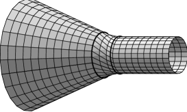
Figure 1: The relativistic gyraton with $m=0$, $j=0.7$ passes through the center of a set of particles initially located at the radius 1. The gravitational field of the gyraton is turned on during the interval $(-1/2,1/2)$ (two solid circular curves). During this interval the particles position is twisted. After this the particles are moving radially outward with a uniform speed.

For this choice the gravitational field of the gyraton affects the particles during the interval $(-1/2,1/2)$. Figure 1 shows the motion of the particles forming the circle for $m=0$ and $j=1$. The initial radius of the circle is chosen to be 1. The coordinate $u$ grows from the right to the left. In this and next figures, two solid circular lines on the surface correspond to the moments $u$ when the gravitational field of the gyraton is switched on ($u_{0}=-1/2$, the right circle) and the moment when it is switched off ($u_{1}=1/2$, the left one). Between these two moments the particles trajectories are twisted. After switching off the gravitational field the particles are moving radially with some positive constant radial velocity.

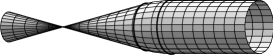
Figure 2: Motion of particles for the gyraton parameters $m=0.25$, $j=0$. For this case there is no twist, and particles move to the center with constant radial velocity. They pass the center, $r=0$ after the gyraton, and passing the caustic starts their expansion.

Figure 2 shows the motion of the particles for the other special case $m=0.25$, $j=0$. As the result of the attraction to the moving gyraton the radius of the circle (which was originally equal to 1) shrinks from its original value. After $u=1/2$ the particles have a constant negative radial velocity. They pass the point $r=0$ some time after the gyraton was there. After a conical caustic at this point the circle starts its linear expansion.

Figure 3: A special case ($m=1$ $j=1$) when the centrifugal repulsion compensates exactly the ”Newtonian” attraction.

Figure 3 illustrates a case when the ”Newtonian” attraction is exactly compensated by the ”centrifugal” repulsion generated by the rotation of the gyraton. After passing the gyraton the particles remain at the same radius $r=r_{0}=1$.

Figure 4: The case when both of the parameters $m$ and $j$ do not vanish, but the attraction dominates ($m=1.5$, $j=1$).

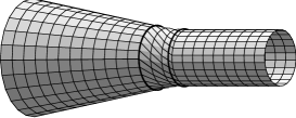
Figure 5: The case when both of the parameters $m$ and $j$ do not vanish, but the repulsion dominates ($m=0.7$, $j=1$).

In the general case either ”Newtonian” attraction or ”centrifugal” repulsion dominates. Figures 5 and 4 illustrate these two options.

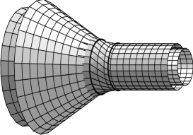
Figure 6: A special case when the repulsion dominates ($m=0$, $j=0.6$). After the gyraton passes throughout the center, the particles located at the inner circle $r_{1}=0.8$ get higher positive radial velocity than the particle which initially were located at $r_{0}=1.0$. The inner particles (their worldsheet is shown by a light surface) cross the outer particles (darker surface). At the moment of the intersection a caustic is formed.

The ”centrifugal force” term is proportional to $r^{-3}$. It means that in the absence of the ”Newtonian” attraction, $\mu=0$, the outward acceleration of particles at smaller radius is bigger than the acceleration at bigger radius. Consider the evolution in time of two circles, one with the original radius $r_{0}$ and the other with $r_{1}<r_{0}$. Since the final positive radial velocity is bigger in the second case, a surface $\Sigma_{1}$ representing the second circle motion (light surface at Figure 6) crosses from the inside the (darker) surface $\Sigma_{0}$ at some moment of time $u$.

In a general case such points of intersection form a caustic curve $u=U(r)$. If the interval during which the field of the gyraton is switched on is much smaller than the time formation of the caustics one can define the function $F$ as follows. Denote by

$$\tilde{j}^{2}=j^{2}\int_{-\infty}^{\infty}du\,\chi^{2}(u)\,.$$ (108)

For the step function $\chi$ given by (106) $\tilde{j}=j$. By integrating the radial equation (99) over a (short) interval when the interaction is switched on and assuming that during this interval the radius remains approximately constant one obtains the following relation

$$\Delta[r^{\prime}]={\tilde{j}^{2}\over r_{0}^{3}}-{m\over r_{0}}\,.$$ (109)

Here $\Delta[r^{\prime}]$ is the change of the radial velocity. In the same approximation

$$\Delta[\phi]={j^{2}\over r_{0}^{2}}\,.$$ (110)

We assume that particles before the gyraton passing nearby were at a fixed radius. After the gyraton has passed, the equation of the particle motion is

$$r=F(r_{0},u)=r_{0}+\left({\tilde{j}^{2}\over r_{0}^{3}}-{m\over r_{0}}\right)u\,.$$ (111)

The condition for caustic formation is $\partial_{r_{0}}F=0$. By solving this equation one obtains the following condition for the caustic line formation

$$u=U(r_{0})={r_{0}^{4}\over 2\tilde{j}^{2}-mr_{0}^{2}}\,.$$ (112)

Substituting this relation into (111) one obtains

$$r={r_{0}(3\tilde{j}^{2}-2mr_{0}^{2})\over 2\tilde{j}^{2}-mr_{0}^{2}}\,.$$ (113)

The equations (112) and (113) describe the caustic equation in the parametric form. Since $r$ must be positive, $r_{0}^{2}\leq 3\tilde{j}^{2}/(2m)$. When $r_{0}$ is close to the limiting value $\sqrt{3}\tilde{j}/\sqrt{2m}$ $u$ becomes

$$u\approx{9\tilde{j}^{2}\over 2m^{2}}\,.$$ (114)

We remind the reader that the above estimations are given in a special frame where the duration of the pulse is 1. Using the scaling law (87) it is possible to rewrite the results in an arbitrary frame where the duration of the pulse is $L$. It is sufficient to notice that under this scaling $m$ and $r$ do not change, while $\tilde{j}\to\tilde{j}/\sqrt{L}$. In particular, under this transformation the relation (112) remains invariant.

Equation (109) allows one to make the following general conclusion. ”Centrifugal” repulsion compensates the ”Newtonian” attraction when

$$r_{0}\sim{j\over\sqrt{mL}}\sim{\sqrt{G}J\over\sqrt{EL}}\,.$$ (115)

It should be emphasized that a realistic beam pulse of spinning radiation has a finite cross section, so that the formulas and approximations used above should be additionally tested for their consistency.

VII Summary and Discussions

Let us summarize the obtained results. The beam-pulses of spinning radiation besides energy have also internal angular momentum. As a result, the metric for the gravitational field of such relativistic gyratons in addition to the ”Newtonian” part contains non-diagonal terms responsible for the gravitomagnetic effects. In the weak field approximation the gravitational field of the relativistic gyraton is related to the boosted Lense-Thirring metric in the limit when the boost parameter is infinitely large. Since the angular momentum in this limit remains finite, the weak field boosted solution is not sufficient to generate an exact solution. In this paper we obtained the exact solutions for the relativistic gyraton in an arbitrary number $D$ of spacetime dimensions. These solutions contain $[D/2]$ arbitrary profile functions of one parameter $u$. They describe the energy density, $\mu(u)$, and angular momentum density, $p_{i}(u)$, along the beam.

When a relativistic gyraton passes near a particle, the motion of the latter is affected by the ”Newtonian” attraction generated by the energy $\mu$ and by an induced ‘centrifugal’ force, generated by the angular momentum of the gyraton. We explicitly demonstrated this for the four-dimensional case but this conclusion is of general nature.

The condition (115) for the radius where repulsive and attractive forces are equal is obtained for classical sources. It is interesting to apply it (at least formally) to the case of a single quantum. For the quantum with wavelength $\lambda$ and spin $s$ one has $E=\hbar/\lambda$ and $J=s\hbar$ and the condition (115) takes the form

$$r_{0}\sim sl_{Pl}\sqrt{{\lambda\over L}}\,.$$ (116)

Here $l_{Pl}=\sqrt{\hbar G}$ is the Planck length. At the threshold of the mini-black-hole production when both the center-of-mass energy of particles and their impact parameter have the Planckian scale, this relation shows that the spin-orbit interaction becomes comparable with the ”Newtonian” attraction for a quantum with $L\sim\lambda$.

In case when both particles have a spin, besides the spin-orbit interaction there exists also an additional spin-spin interaction. One can expect that both effects might be important in the Planckian regime and change the estimated cross-section of mini black hole formation. In order to study this problem one needs to find the metric for ultra-relativistic particles with a spin. The solutions obtained in this paper for the relativistic gyraton can be a good starting point in this investigation.

Appendix A Boost of a compact source

In the case when $\chi(u)=\chi_{i}(u)=\delta(u)$ metric (50)–(52) can be obtained from the metric of a source by the boost. Consider a compact source in a flat space-time which is at rest in the frame of reference with coordinates $\bar{x}^{\mu}$, such that $\bar{x}^{1}=\bar{t}$ ($\bar{t}$ is time coordinate) $\bar{x}^{2}=\bar{\xi}$, $\bar{x}^{a}=x^{a}$, $a=3,..,D$. We call $x^{a}$ transverse coordinates and denote them by the vector ${\bf x}_{\perp}$. The source has the mass

$$M=\int d\bar{\xi}d{\bf x}_{\perp}T_{00}~{}~{},$$

and the angular momentum tensor

$$J_{\mu\nu}=\int d\bar{\xi}d{\bf x}_{\perp}(x^{\mu}T^{\nu}_{0}-x^{\nu}T^{\mu}_{0})~{}~{},$$

where $T_{\mu\nu}$ is the stress-energy tensor of the source. It is assumed that the source rotates only in transverse directions, hence the only non-trivial components of the angular momentum tensor are $J_{ab}$. The number of rotation bi-planes is $l=[(D-2)/2]$. As before we work in the transverse coordinates corresponding to the rotation bi-planes, where $J_{ab}$ has a block-diagonal form, and denote $J_{i}$ the momentum in the $i$-th bi-plane.

In the weak field approximation the gravitational field of the source is given by the metric MyPe

$$ds^{2}=-d\bar{t}^{2}+d\bar{\xi}^{2}+d{\bf x}_{\perp}^{2}+$$

$$2\tilde{\Phi}\,\left(d\bar{t}^{2}+{1\over D-3}(d\bar{\xi}^{2}+d{\bf x}_{\perp}^{2})\right)+$$

$$2d\bar{t}\sum_{i=1}^{l}\tilde{A}_{i}\,(y_{i}dx_{i}-x_{i}dy_{i})\,,$$ (117)

where

$$d{\bf x}_{\perp}^{2}=\sum_{i=1}^{l}(dx_{i}^{2}+dy_{i}^{2})+\epsilon dz^{2}~{}~{},$$

$$\tilde{\Phi}(\rho)=-{\kappa M(D-3)\over 2(D-2)\Omega_{D-2}}f_{D-3}(\rho)~{}~{},$$ (118)

$$\tilde{A}_{i}(\rho)=-{\kappa\over 4\Omega_{D-2}}{J_{i}\over\rho^{D-1}}~{}~{}.$$ (119)

Functions $f_{D-3}$ are defined by (41),

$$\rho^{2}=\bar{\xi}^{2}+{\bf x}_{\perp}^{2}=\bar{\xi}^{2}+R^{2}~{}~{}~{},$$

and $\epsilon=0$ if the number of transverse directions is even.

Let us go to a frame of reference which moves backwards along $\xi$-axis with the velocity $\beta$ (we work in the system of units where the velocity of light $c=1$). Let $\xi$, $t$, $u=t-\xi$, $v=t+\xi$ be the corresponding coordinates in the moving frame,

$$\bar{\xi}=\gamma(\xi-\beta t)~{}~{},~{}~{}\bar{t}=\gamma(t-\beta\xi)~{}~{},$$ (120)

where $\gamma=(1-\beta^{2})^{-1/2}$. By using (120) one can consider the limit $\beta\rightarrow 1$. In this limit the source is moving with respect to the new frame of reference with the velocity of light. Let $\triangle_{\perp}$ be the Laplace operator in the transverse directions and

$$\triangle=\triangle_{\perp}+\partial_{\bar{\xi}}^{2}~{}~{}.$$ (121)

In the limit of infinite boost operators $\triangle$ and $\triangle_{\perp}$ coincide up to terms $O(\gamma^{-2})$. According to definitions of Green’s functions (39), (40),

$$\triangle f_{D-3}(\rho)=\Omega_{D-2}\delta(\bar{\xi})\delta({\bf x}_{\perp})~{}~{},$$ (122)

$$\triangle_{\perp}f_{D-4}(R)=\Omega_{D-3}\delta({\bf x}_{\perp})~{}~{}.$$ (123)

In the limit of infinite boost the following relations hold

$$\lim_{\beta\rightarrow 1}(\gamma f_{1}(\rho))=f_{1}(u)+2\delta(u)f_{0}(R)~{}~{},$$ (124)

$$\lim_{\beta\rightarrow 1}(\gamma f_{D-3}(\rho))=\delta(u){\Omega_{D-2}\over\Omega_{D-3}}f_{D-4}(R)~{}~{},~{}~{}D>4~{}~{},$$ (125)

$$\lim_{\beta\rightarrow 1}\left(\gamma{x_{i}\over\rho^{D-1}}\right)=$$

$$\lim_{\beta\rightarrow 1}\left(\gamma\partial_{x_{i}}f_{D-3}(\rho)\right)=\delta(u){\Omega_{D-2}\over\Omega_{D-3}}{x_{i}\over R^{D-2}}~{}~{},$$ (126)

which can be found with the help of (122), (123) if one has takes into account that $\lim_{\beta\rightarrow 1}(\gamma\delta(\bar{\xi}))=\delta(u)$.

By using (124)–(126) one finds that in the limit of the infinite boost metric (117) takes the form (50)–(52) provided that the mass of the source behaves in this limit as

$$M={E\over\gamma}$$

while components of the angular momentum $J_{i}$ remain finite. To get the gyraton metric (86) from the boost in four dimensions one has to make an additional coordinate transformation $\tilde{v}=v-4GE\ln u/u_{0}$, where $u_{0}$ is a constant.

Appendix B Metric ansatz and curvature calculations

B.1 General formulas

We define the metric to be

$$ds^{2}=\eta_{(\mu)(\nu)}\omega^{(\mu)}\omega^{(\nu)}\,.$$ (127)

Here $\omega^{(\mu)}=\omega^{(\mu)}_{\nu}dx^{\nu}$ are basic forms and $\eta_{(\mu)(\nu)}$ is a non-degenerate matrix with constant coefficients. We denote $e_{(\mu)}=e_{(\mu)}^{\nu}\partial_{\nu}$ basic vectors dual to the basic forms

$$e_{(\mu)}^{\nu}\omega^{(\lambda)}_{\nu}=\delta^{(\mu)}_{(\lambda)}\,.$$ (128)

Let us define

$$\lambda_{(\mu)(\nu)(\lambda)}=e_{(\mu)}^{\epsilon}e_{(\lambda)}^{\rho}[\omega_{(\nu)\epsilon,\rho}-\omega_{(\nu)\rho,\epsilon}]\,.$$ (129)

These coefficients possess the following property

$$\lambda_{(\mu)(\nu)(\lambda)}=-\lambda_{(\lambda)(\nu)(\mu)}\,.$$ (130)

The Ricci rotation coefficients are defined as

$$\gamma_{(\mu)(\nu)(\lambda)}={1\over 2}[\lambda_{(\mu)(\nu)(\lambda)}+\lambda_{(\lambda)(\mu)(\nu)}-\lambda_{(\nu)(\lambda)(\mu)}]\,.$$ (131)

The Riemann tensor can be written by using the Ricci rotation coefficients as follows (see e.g. Chand )

$$R_{(\mu)(\nu)(\lambda)(\rho)}=-\gamma_{(\mu)(\nu)(\lambda),(\rho)}+\gamma_{(\mu)(\nu)(\rho),(\lambda)}$$

$$+\gamma_{(\nu)(\mu)(\epsilon)}[\gamma_{(\lambda)\ (\rho)}^{\ \ (\epsilon)}-\gamma_{(\rho)\ (\lambda)}^{\ \ (\epsilon)}]$$ (132)

$$+\gamma_{(\epsilon)(\mu)(\lambda)}\gamma_{(\nu)\ (\rho)}^{\ \ (\epsilon)}-\gamma_{(\epsilon)(\mu)(\rho)}\gamma_{(\nu)\ (\lambda)}^{\ \ (\epsilon)}\,.$$

Here $(\ldots)_{,(\mu)}=e^{\nu}_{(\mu)}(\ldots)_{,\nu}$. Finally the Ricci tensor is

$$R_{(\mu)(\lambda)}=\eta^{(\nu)(\rho)}R_{(\mu)(\nu)(\lambda)(\rho)}\,.$$ (133)

B.2 Even-dimensional space-time

Formulas for even and odd dimensional cases are slightly different. Consider first the even dimensional case and denote $l=(D-2)/2$. We shall use two real coordinates, $x^{1}=u$ and $x^{2}=v$. The other coordinates $x^{a}$, $a=3,\ldots,D$ are complex. We shall use the following notations for this set of complex coordinate $x^{i}=\zeta^{i}$, $x^{\bar{i}}=\bar{\zeta}^{i}$, where $i=3,5,\ldots,2l+1$ and $\bar{i}=i+1$. In this notations a partial derivative $A_{,a}$ denotes the following set of partial derivatives

$$A_{,i}=\partial_{\zeta^{i}}A\,,\hskip 14.22636ptA_{,\bar{i}}=\partial_{\bar{\zeta}^{i}}A\,.$$ (134)

We shall use the same convention for the indices connected with the basic vectors and forms. We denote

$$\eta^{ab}=\sum_{i}[\delta^{a}_{i}\delta^{b}_{\bar{i}}+\delta^{a}_{\bar{i}}\delta^{b}_{i}]\,.$$ (135)

Using this notation we can write the metric in the form

$$ds^{2}=-2\omega^{(1)}\omega^{(2)}+2\sum_{i}\omega^{(i)}\bar{\omega}^{(i)}\,.$$ (136)

We adopt the following ansatz for the metric. Let us denote

$$\omega^{(1)}=du\,,\hskip 14.22636pt\omega^{(2)}=\frac{1}{2}dv-Qdu\,,$$ (137)

$$\omega^{(i)}=d\zeta^{i}+{W}^{i}du\,,\hskip 14.22636pt\omega^{(\bar{i})}\equiv\bar{\omega}^{(i)}=d\bar{\zeta}^{i}+\bar{W}^{i}du\,.$$ (138)

Here $Q=Q(u,\zeta_{i},\bar{\zeta}_{i})$ and $W^{i}=W^{i}(u,\zeta_{i},\bar{\zeta}_{i})$. We also define

$$W_{i}={W}^{\bar{i}}=\bar{W}^{i}\,,\hskip 14.22636ptW_{\bar{i}}=\bar{W}_{i}={W}^{i}\,.$$ (139)

The differentials of the coordinates can be expressed in terms of basic forms as follows

$$du=\omega^{(1)}\,,\hskip 14.22636ptdv=2(\omega^{(2)}+Q\omega^{(1)})\,,$$ (140)

$$d\zeta^{i}=\omega^{(i)}-{W}^{i}\omega^{(1)}\,,\hskip 14.22636ptd\bar{\zeta}^{i}=\bar{\omega}^{(i)}-\bar{W}^{i}\bar{\omega}^{(1)}\,.$$ (141)

The corresponding vector basis is

$$e_{(1)}=\partial_{u}-{\cal D}+2Q\partial_{v}\,,\hskip 14.22636pte_{(2)}=2\partial_{v}\,,$$ (142)

$$e_{(i)}=\partial_{\zeta^{i}}\,,\hskip 14.22636pte_{(\bar{i})}\equiv\bar{e}_{(i)}=\partial_{\bar{\zeta}^{i}}\,,$$ (143)

$${\cal D}=\sum_{i}({W}^{i}\partial_{\zeta^{i}}+\bar{W}^{i}\partial_{\bar{\zeta}^{i}})\,.$$ (144)

The metric is

$$ds^{2}=-dudv+2\sum_{i}d\zeta^{i}d\bar{\zeta}^{i}+2(Q+\sum_{i}W_{i}W_{\bar{i}})du^{2}\,.$$

$$+2\sum_{i}(W_{i}d\zeta^{i}+W_{\bar{i}}d\bar{\zeta}^{i})du\,.$$ (145)

Calculations give the following non-vanishing components of $\lambda_{(\mu)(\nu)(\lambda)}$

$$\lambda_{(1)(1)(a)}=Q_{,a}\,.$$ (146)

$$\lambda_{(1)(a)(b)}=W_{a,b}\,.$$ (147)

Non-vanishing components of the rotation coefficients are

$$\gamma_{(1)(a)(1)}=Q_{,a}\,,$$ (148)

$$\gamma_{(1)(a)(b)}={1\over 2}(W_{a,b}+W_{b,a})\,,$$ (149)

$$\gamma_{(a)(b)(1)}={1\over 2}(W_{a,b}-W_{b,a})\,,$$ (150)

Notice that the rotation coefficients do not vanish only if their first or the third index is equal to 1. If any of its indices is 2 the rotation coefficient vanishes. Using these properties and the definition of the Ricci tensor (133) it is possible to show that

$$R_{(a)(b)}=R_{(2)(a)}=R_{(a)(2)}=0\,.$$ (151)

Non-vanishing coefficients of the Ricci tensor are

$$R_{(1)(1)}=-\bigtriangleup Q+Z_{,u}-{\cal D}Z-U\,,$$ (152)

$$R_{(1){a}}=-{1\over 2}\bigtriangleup W_{a}+{1\over 2}Z_{,a}\,.$$ (153)

Here $\bigtriangleup=\eta^{ab}\partial_{a}\partial_{b}$ and

$$Z=\eta^{ab}W_{a,b}=\sum_{i}(W_{i,\bar{i}}+W_{\bar{i},i})\,,$$ (154)

$$U={1\over 2}(\eta^{ac}\eta^{bd}+\eta^{ad}\eta^{bc})W_{a,b}W_{c,d}\,.$$ (155)

To obtain a solution we choose

$$W_{i}=-ip_{i}{\bar{\zeta}^{i}\over R^{2l}}\,,$$ (156)

$$R^{2}=2\sum_{i}\zeta^{i}\bar{\zeta}^{i}\,.$$ (157)

Here $p_{i}=p_{i}(u)$ are arbitrary functions of $u$. We demonstrate now that for this choice the components $R_{(1)(a)}$ of Ricci tensor vanish.

It is easy to check that

$$W_{i,j}=2ilp_{i}{\bar{\zeta}^{i}\bar{\zeta}^{j}\over R^{2(l+1)}}\,,$$ (158)

$$W_{\bar{i},\bar{j}}=-2ilp_{i}{{\zeta}^{i}{\zeta}^{j}\over R^{2(l+1)}}\,,$$ (159)

$$W_{i,\bar{j}}={i\over R^{2l}}\left[2lp_{i}{\bar{\zeta}^{i}{\zeta}^{j}\over R^{2}}-p_{i}\delta_{ij}\right]\,,$$ (160)

$$W_{\bar{i},{j}}=-{i\over R^{2l}}\left[2lp_{i}{{\zeta}^{i}\bar{\zeta}^{j}\over R^{2}}-p_{i}\delta_{ij}\right]\,.$$ (161)

It is easy to see that for each $i$, $W_{i,\bar{i}}+W_{\bar{i},i}=0$, and hence $Z=0$. We also have (outside a singular point $R=0$)

$$\bigtriangleup\left({1\over R^{2m}}\right)={4m(m-l+1)\over R^{2(m+1)}}\,,$$ (162)

$$\bigtriangleup\left({\zeta^{i}\over R^{2m}}\right)={4m(m-l)\zeta^{i}\over R^{2(m+1)}}\,,$$ (163)

$$\bigtriangleup\left({\zeta^{i}\bar{\zeta}^{i}\over R^{2m}}\right)={2\over R^{2m}}\left[1+{2m(m-l-1)\zeta^{i}\bar{\zeta}^{i}\over R^{2}}\right]\,.$$ (164)

The equation (163) implies

$$\bigtriangleup W_{i}=\bigtriangleup W_{\bar{i}}=0\,.$$ (165)

Thus $R_{(1)(a)}=0$ and $R_{(1)(1)}$ takes the form

$$R_{(1)(1)}=-(\bigtriangleup Q+U)\,.$$ (166)

The metric (145) is a vacuum solution if the function $Q$ obeys the equation

$$\bigtriangleup Q=-U\,.$$ (167)

It is convenient to rewrite expression (155) for $U$ in the form

$$U=U_{+}+U_{-}\,,$$ (168)

where

$$U_{+}={1\over 2}(W_{i,j}+W_{j,i})(W_{\bar{i},\bar{j}}+W_{\bar{j},\bar{i}})\,,$$ (169)

$$U_{-}={1\over 2}(W_{\bar{i},j}+W_{j,\bar{i}})(W_{i,\bar{j}}+W_{\bar{j},i})\,.$$ (170)

The calculations give

$$U_{\pm}={l^{2}\over R^{4l+4}}(R^{2}P^{2}\pm I^{2})\,,$$ (171)

Here

$$P^{2}=2\sum_{i}p_{i}^{2}\zeta^{i}\bar{\zeta}^{i}\,,$$ (172)

$$I=2\sum_{i}p_{i}\zeta_{i}\bar{\zeta}^{i}\,.$$ (173)

Combining these relations one obtains

$$U={2l^{2}P^{2}\over R^{4l+2}}\,.$$ (174)

We write a solution $Q$ of the equation

$$\bigtriangleup Q=-U\,,$$ (175)

as a sum

$$Q=\Phi+\Psi\,,$$ (176)

where $\Psi$ is a special solution of the inhomogeneous equation (175) and $\Phi$ is an arbitrary solution of the homogeneous equation

$$\bigtriangleup\Phi=0\,.$$ (177)

Relation (162) implies that

$$\Phi={\mu(u)\over R^{2(l-1)}}$$ (178)

with an arbitrary function $\mu(u)$.

To find a solution of the inhomogeneous equation we use the ansatz

$$\Psi=a_{l}{P^{2}\over R^{4l}}+b_{l}{p^{2}\over R^{4l-2}}\,,$$ (179)

where

$$p^{2}=\sum_{i}p_{i}^{2}\,.$$ (180)

Using relations (162) and (164) one has

$$\bigtriangleup\Psi={1\over R^{4l}}\left[A_{l}{P^{2}\over R^{2}}+B_{l}p^{2}\right]\,,$$ (181)

$$A_{l}=8l(l-1)a_{l}\,,\hskip 14.22636ptB_{l}=4a_{l}+4l(2l-1)b_{l}\,.$$ (182)

Equations (174) and (175) give

$$a_{l}=-{l\over 4(l-1)}\,,\hskip 14.22636ptb_{l}={1\over 4(l-1)(2l-1)}\,.$$ (183)

Let us denote

$${\cal B}=2\Psi+2\sum_{i}W_{i}\bar{W}_{i}\,.$$ (184)

Since

$$\sum_{i}W_{i}\bar{W}_{i}={P^{2}\over 2R^{4l}}\,,$$ (185)

one has

$${\cal B}={1\over R^{4l-2}}\left[\alpha_{l}{P^{2}\over R^{2}}+\beta_{l}p^{2}\right]\,,$$ (186)

where

$$\alpha_{l}={l-2\over 2(l-1)}\,,\hskip 14.22636pt\beta_{l}={1\over 2(l-1)(2l-1)}\,.$$ (187)

B.3 Odd-dimensional space-time

In the case of an odd dimensional space-time the calculations are similar. We shall briefly give the main results omitting the details.

Let us denote $l=(D-3)/2$. As earlier we use 2 real coordinates, $x^{1}=u$, $x^{2}=v$. We denote the other coordinates by $x^{a}$, $a=3,\ldots,D$. They consist of $l$ sets of complex conjugated coordinates $x^{i}=\zeta^{i}$, $x^{\bar{i}}=\bar{\zeta}^{i}$, where $i=3,5,\ldots,2l+1$ and $\bar{i}=i+1$, and one additional real coordinate, which we denote by $z$, $x^{2l+3}=z$.

In this notations a partial derivative $A_{,a}$ denotes the following set of partial derivatives

$$A_{,i}=\partial_{\zeta^{i}}A\,,\hskip 14.22636ptA_{,\bar{i}}=\partial_{\bar{\zeta}^{i}}A\,,\hskip 14.22636ptA_{,z}=\partial_{z}A\,.$$ (188)

We shall use the same convention for the indices connected with the basic vectors and forms. We denote

$$\eta^{ab}=\sum_{i}[\delta^{a}_{i}\delta^{b}_{\bar{i}}+\delta^{a}_{\bar{i}}\delta^{b}_{i}]+\delta^{a}_{z}\delta^{b}_{\bar{z}}\,.$$ (189)

Using this notation we can write the metric in the form

$$ds^{2}=-2\omega^{(1)}\omega^{(2)}+2\sum_{i}\omega^{(i)}\bar{\omega}^{(i)}+(\omega^{(z)})^{2}\,.$$ (190)

The basic forms $\omega^{(1)}$, $\omega^{(2)}$, $\omega^{(i)}$ and $\bar{\omega}^{(i)}$ are given by (137)–(138) with $Q=Q(u,\zeta_{i},\bar{\zeta}_{i},z)$ and $W^{i}=W^{i}(u,\zeta_{i},\bar{\zeta}_{i},z)$ and

$$\omega^{(z)}=dz\,.$$ (191)

The metric is

$$ds^{2}=-dudv+2\sum_{i}d\zeta^{i}d\bar{\zeta}^{i}+dz^{2}\,.$$

$$+2\sum_{i}(W_{i}d\zeta^{i}+W_{\bar{i}}d\bar{\zeta}^{i})du+2(Q+\sum_{i}W_{i}W_{\bar{i}})du^{2}\,.$$ (192)

It is convenient to denote $W_{a}$ an object which besides the components $W_{i}$ and $W_{\hat{i}}$ has one more additional component $W_{z}=0$. Using these notations it is possible to show that the non-vanishing components of $\lambda_{(\mu)(\nu)(\lambda)}$ and $\gamma_{(\mu)(\nu)(\lambda)}$ are given by relations (146)–(150). For the non-vanishing components of the Ricci tensor one has

$$R_{(1)(1)}=-\bigtriangleup Q+Z_{,u}-{\cal D}Z-U\,,$$ (193)

$$R_{(1){a}}=-{1\over 2}\bigtriangleup W_{a}+{1\over 2}Z_{,a}\,.$$ (194)

Here

$${\cal D}=\sum_{i}({W}^{i}\partial_{\zeta^{i}}+\bar{W}^{i}\partial_{\bar{\zeta}^{i}})\,,$$ (195)

$$\bigtriangleup=\eta^{ab}\partial_{a}\partial_{b}=2\sum_{i}\partial_{\zeta^{i}}\partial_{\bar{\zeta}^{i}}+\partial^{2}_{z}\,,$$ (196)

$$Z=\eta^{ab}W_{a,b}=\sum_{i}(W_{i,\bar{i}}+W_{\bar{i},i})\,,$$ (197)

$$U={1\over 2}(\eta^{ac}\eta^{bd}+\eta^{ad}\eta^{bc})W_{a,b}W_{c,d}\,.$$ (198)

To obtain a solution we choose

$$W_{i}=-ip_{i}{\bar{\zeta}^{i}\over R^{(2l+1)}}\,,$$ (199)

$$R^{2}=2\sum_{i}\zeta^{i}\bar{\zeta}^{i}+z^{2}\,.$$ (200)

Here $\mu(u)$ and $p_{i}=p_{i}(u)$ are arbitrary functions of $u$. We demonstrate now that for this choice the components $R_{(1)(a)}$ of Ricci tensor vanish.

It is easy to check that

$$W_{i,j}=i(2l+1)p_{i}{\bar{\zeta}^{i}\bar{\zeta}^{j}\over R^{(2l+3)}}\,,$$ (201)

$$W_{\bar{i},\bar{j}}=-i(2l+1)p_{i}{{\zeta}^{i}{\zeta}^{j}\over R^{(2l+3)}}\,,$$ (202)

$$W_{i,\bar{j}}={i\over R^{(2l+1)}}\left[(2l+1)p_{i}{\bar{\zeta}^{i}{\zeta}^{j}\over R^{2}}-p_{i}\delta_{ij}\right]\,,$$ (203)

$$W_{\bar{i},{j}}=-{i\over R^{(2l+1)}}\left[(2l+1)p_{i}{{\zeta}^{i}\bar{\zeta}^{j}\over R^{2}}-p_{i}\delta_{ij}\right]\,.$$ (204)

$$W_{i,z}=i(2l+1)p_{i}{\bar{\zeta}^{i}z\over R^{(2l+3)}}\,,$$ (205)

$$W_{\bar{i},z}=-i(2l+1)p_{i}{\zeta^{i}z\over R^{(2l+3)}}\,.$$ (206)

It is easy to see that for each $i$, $W_{i,\bar{i}}+W_{\bar{i},i}=0$, and hence $Z=0$. We also have (outside a singular point $R=0$)

$$\bigtriangleup\left({1\over R^{2m}}\right)={2m(2m-2l+1)\over R^{2(m+1)}}\,,$$ (207)

$$\bigtriangleup\left({\zeta^{i}\over R^{2m}}\right)={2m(2m-2l-1)\zeta^{i}\over R^{2(m+1)}}\,,$$ (208)

$$\bigtriangleup\left({\zeta^{i}\bar{\zeta}^{i}\over R^{2m}}\right)={2\over R^{2m}}\left[1+{m(2m-2l-3)\zeta^{i}\bar{\zeta}^{i}\over R^{2}}\right]\,,$$ (209)

$$\bigtriangleup\left({z^{2}\over R^{2m}}\right)={2\over R^{2m}}\left[1+{m(2m-2l-3)z^{2}\over R^{2}}\right]\,.$$ (210)

The equation (208) implies

$$\bigtriangleup W_{i}=\bigtriangleup W_{\bar{i}}=0\,.$$ (211)

Thus $R_{(1)(a)}=0$ and $R_{(1)(1)}$ takes the form

$$R_{(1)(1)}=-(\bigtriangleup Q+U)\,.$$ (212)

The metric (192) is a vacuum solution if the function $Q$ obeys the equation

$$\bigtriangleup Q=-U\,.$$ (213)

The function $U$ defined by (155) can be rewritten as

$$U=U_{+}+U_{-}+U_{0}\,,$$ (214)

where $U_{\pm}$ are defined by (169) and (170) and

$$U_{0}=\sum_{i}W_{i,z}W_{\bar{i},z}\,.$$ (215)

The calculations give

$$U_{\pm}={(2l+1)^{2}\over 4R^{4l+6}}[P^{2}(R^{2}-z^{2})\pm I^{2}]\,,$$ (216)

$$U_{0}={(2l+1)^{2}\over 2R^{4l+6}}P^{2}z^{2}\,.$$ (217)

Thus one has

$$U={(2l+1)^{2}P^{2}\over 2R^{4l+4}}\,.$$ (218)

We write a solution $Q$ of (213) in the form (176), $Q=\Phi+\Psi$, where as earlier $\Phi$ is a solution of the homogeneous equation and $\Psi$ is a special solution of the inhomogeneous one. Relation (207) implies that

$$\Phi={\mu(u)\over R^{2l-1}}\,,$$ (219)

where $\mu(u)$ is an arbitrary function of $u$.

To find a solution of the inhomogeneous equation we use the ansatz anz

$$\Psi=a_{l}{P^{2}\over R^{4l+2}}+b_{l}{p^{2}\over R^{4l}}\,.$$ (220)

Using relations (162) and (164) one has

$$\bigtriangleup\Psi={1\over R^{4l+2}}\left[A_{l}{P^{2}\over R^{2}}+B_{l}p^{2}\right]\,,$$ (221)

$$A_{l}=2(4l^{2}-1)a_{l}\,,\hskip 14.22636ptB_{l}=4a_{l}+4l(2l+1)b_{l}\,.$$ (222)

Equations (213) and (218) give

$$a_{l}=-{(2l+1)\over 4(2l-1)}\,,\hskip 14.22636ptb_{l}={1\over 4l(2l-1)}\,.$$ (223)

Let us denote

$${\cal B}=2\Psi+2\sum_{i}W_{i}\bar{W}_{i}\,.$$ (224)

Since

$$\sum_{i}W_{i}\bar{W}_{i}={P^{2}\over 2R^{4l+2}}\,,$$ (225)

one has

$${\cal B}={1\over R^{4l}}\left[\alpha_{l}{P^{2}\over R^{2}}+\beta_{l}p^{2}\right]\,,$$ (226)

where

$$\alpha_{l}={2l-3\over 2(2l-1)}\,,\hskip 14.22636pt\beta_{l}={1\over 2l(2l-1)}\,.$$ (227)

References

• (1) P.C. Aichelburg and R.U. Sexl, Gen. Rel. Grav. 2 (1971) 303.
• (2) C. Barrabès and P. A. Hogan, Singular Null Hypersurfaces in General Relativity, World Scientific, 2003.
• (3) For a review of works studying the Penrose limit in string theory see, e.g., J.C. Plefka, Lectures on Plane-Wave String/Gauge Theory Duality, hep-th/0307101; D. Sadri, M.M. Sheikh-Jabbari, The Plane-Wave/Super Yang-Mills Duality, hep-th/0310119.
• (4) P. Kanti, Int.J.Mod.Phys. A19 4899 (2004).
• (5) D.M. Eardley and S.B. Giddings, Phys. Rev. 66 (2002) 044011.
• (6) H. Yoshino and Y. Nambu, Phys.Rev. D66 065004 (2002).
• (7) H. Yoshino and Y. Nambu, Phys.Rev. D67 024009 (2003).
• (8) H. Yoshino and V. Rychkov, Improved Analysis of Black Hole Formation in High-Energy Particle Collisions, hep-th/0503171.
• (9) C. Barrabés, V. Frolov, and E. Lesigne, Phys.Rev. D69 101501 (2004).
• (10) V. Frolov and D. Stojkovic, Phys.Rev.Lett 89 151302 (2002).
• (11) V. Frolov and D. Stojkovic, Phys.Rev. D66 084002 (2002).
• (12) D. Ida, Kin-ya Oda, and S. C. Park, Phys.Rev. D67 064025 (2003).
• (13) E. Jung, S. H. Kim, and D.K. Park, e-Print Archive: hep-th/0503163 (2005).
• (14) V. Ferrari and P. Pendenza, GRG 22 1105 (1990).
• (15) N. Sanchez and C. Lousto, Nucl.Phys. B383 377 (1992).
• (16) H. Balasin and H. Nachbagauer, Class.Quant.Grav. 12 707 (1995).
• (17) H. Balasin and H. Nachbagauer, Class.Quant.Grav. 13 731 (1996).
• (18) A. Burinskii and G. Magli, Phys. Rev. D61 (2000) 044017.
• (19) C. Barrabés and P.A. Hogan, Phys.Rev. D67 084028 (2003).
• (20) C. Barrabés and P.A. Hogan, Phys.Rev. D70 107502 (2004).
• (21) H. Yoshino, Phys.Rev. D71 044032 (2005).
• (22) Tensor $M^{\sigma\rho}_{\nu}$ in (15) differes from the angular momentum tensor derived with the help of the Noether theorem by the term $\partial^{\lambda}Q^{\sigma\rho}_{\lambda\nu}$, where $Q^{\sigma\rho}_{\lambda\nu}=F_{\lambda\nu}(A^{\sigma}x^{\rho}-A^{\rho}x^{\sigma})$. This addition does not contribute to the integral of the angular momentum.
• (23) A general theory of the narrow beams in the quasiclassical approximation can be found in: V.P. Maslov, The Complex WKB Method for Nonlinear Equations, Moscow, Nauka, (1977); English transl.: The Complex WKB Method for Nonlinear Equations. I. Linear Theory, Basel, Boston, Berlin, Birkhauser Verlag (1994).
• (24) F. R. Gantmacher, The Theory of Matrices, American Mathematical Society (1998).
• (25) To simplify expressions, in this section we use notations slightly different from those adopted in appendix B. Namely, the index $i$ takes values $i=1,\ldots,l$. We also use complex coordinates $z^{i}$ related to $\zeta^{i}$ as follows $z^{i}=\zeta^{2i+1}$ and $\bar{z}^{i}=\bar{\zeta}^{2i+1}=\zeta^{2i+2}$.
• (26) B. Mashhoon, Gravitoelectromagnetism: A brief review, e-Print gr-qc/0311030 (2003).
• (27) H. Stephani et al, Exact solutions to Einstein’s Field Equations, second edition, Chapter 31, Cambridge monographs on mathematical physics, Cambridge Univesity Press (2003).
• (28) R.C. Myers and M.J. Perry, Annals of Phys. 172 (1986) 304.
• (29) S. Chandrasekhar, The Mathematical Theory of Black Holes, University of Chicago, Oxford Univ. Press, 1983.
• (30) In order to make the ansatz more general, one may add to the expression for $\Psi$ an additional term of the form $c_{l}z^{2}/R^{4l+2}$. Using (210) one can see that a similar term would appear in $\bigtriangleup\Psi$. The other terms in $\Psi$ do not generate such a term, and $U$ does not contain it. Thus it is possible to conclude that $c_{l}=0$.