Fermionic determinant for dyons and instantons with nontrivial holonomy

Abstract

We calculate exactly the functional determinant for fermions in fundamental representation of $SU(2)$ in the background of periodic instanton with non-trivial value of the Polyakov line at spatial infinity. The determinant depends on the value of the holonomy ${\rm v}$, the temperature, and the parameter $r_{12}$, which at large values can be treated as separation between the Bogomolny–Prasad–Sommerfeld monopoles (or dyons) which constitute the periodic instanton. We find a compact expression for small and large $r_{12}$ and compute the determinant numerically for arbitrary $r_{12}$ and ${\rm v}$.

I Introduction

It is well-known that QCD with light fermions has a chiral symmetry restoration phase transition at the temperature $T\simeq 170$ MeV. This phase transition has been studied on the lattice and with the help of various QCD-motivated models (see, for example Kogut ; Fleming , Berges ), however, not much is known about its driving mechanism.

When the temperature is high the effective coupling constant becomes small and the theory can be studied semiclassically. From the other side, at zero temperature it is very likely that the instanton – anti-instanton ensemble (the instanton liquid) is responsible for the spontaneous chiral symmetry breaking DP2a ; DP2b ; DP3 ; Dobzor . Therefore, in order to get an insight into the mechanism of chiral symmetry breaking and restoration at non-zero temperatures, it is natural to consider an ensemble of the (anti) self-dual fields at finite temperature. A generalization of the usual Belavin–Polyakov–Schwartz–Tyupkin (BPST) instantons BPST for arbitrary temperatures is the Kraan–van Baal–Lee–Lu (KvBLL) caloron with non-trivial holonomy KvB ; LL . These configuration were extensively studied on the lattice in  Brower ; IMMPSV ; Gatt for $SU(2)$ and $SU(3)$ gauge groups. To construct an ensemble of these configurations theoretically, one should first compute the quantum weight of the single KvBLL caloron, or the probability with which this configuration occurs in the partition function of the theory. In Ref. DGPS this problem was solved for the pure Yang–Mills theory. To extend that result to the theory with fermions one has to calculate the fermionic determinant in the background of the KvBLL caloron. This calculation is the aim of the present paper.

Speaking of finite temperature one implies that the Euclidean space-time is compactified in the ‘time’ direction whose inverse circumference is the temperature $T$, with the usual periodic boundary conditions for boson fields and anti–periodic conditions for the fermion fields. In particular, it means that the gauge field is periodic in time, and the theory is no longer invariant under arbitrary gauge transformations, but only under gauge transformations that are periodical in time. As the space topology becomes nontrivial the number of gauge invariants increases. The new invariant is the holonomy or the eigenvalues of the Polyakov line that winds along the compact ’time’ direction Polyakov

$$L=\left.{\rm P}\,\exp\left(\int_{0}^{1/T}\!dt\,A_{4}\right)\right|_{|\vec{x}|\to\infty}.$$ (1)

This invariant together with the topological charge and the magnetic charge can be used for the classification of the field configurations GPY its zero vacuum average is one of the common criteria of confinement.

The general expression for the self-dual electrically neutral configuration with topological charge $1$ and arbitrary holonomy was constructed a few years ago by Kraan and van Baal KvB and Lee and Lu LL ; it has been named the KvBLL caloron. In the limiting case, when the KvBLL caloron is characterized by trivial holonomy (meaning that the Polyakov line (1) assumes values belonging to the group center $Z(N)$ for the $SU(N)$ gauge group), it is reduced to the periodic Harrington-Shepard HS caloron known before. In this limit the quantum weights were studied in detail by Gross, Pisarski and Yaffe GPY .

Besides the neutral self-dual configurations there are charged configurations. The “elementary” soliton with unit electric and magnetic charges is the dyon, also called the Bogomolnyi–Prasad–Sommerfeld (BPS) monopole Bog ; PS . It is a self-dual solution of the Yang–Mills equations of motion with static (i.e. time-independent) action density, which carries both the magnetic and electric fields of the Coulomb type at infinity, decaying as $1/r^{2}$. In the $SU(2)$ gauge theory there are in fact two types of self-dual dyons LY $M$ and $L$ with (electric, magnetic) charges $(+,+)$ and $(-,-)$, and two types of anti-self-dual dyons $\overline{M}$ and $\overline{L}$ with charges $(+,-)$ and $(-,+)$, respectively. Formally, $L$ and $M$ dyons are related by a non-periodical gauge transformation.

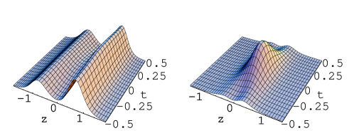
Figure 1: The action density of the KvBLL caloron as function of $z,t$ at fixed $x=y=0$, with the asymptotic value of $A_{4}$ at spatial infinity ${\rm v}=0.9\pi T,\;\overline{{\rm v}}=1.1\pi T$. It is periodic in $t$ direction. At large dyon separation the density becomes static (left, $r_{12}=1.5/T$). As the separation decreases the action density becomes more like a $4d$ lump (right, $r_{12}=0.6/T$). In both plots the L,M dyons are centered at $z_{\rm L}=-{\rm v}\,r_{12}/2\pi T,\;z_{\rm M}=\overline{{\rm v}}\,r_{12}/2\pi T,\;x_{\rm L,M}=y_{\rm L,M}=0$. The axes are in units of temperature T.

The KvBLL caloron of the $SU(2)$ gauge group (to which we restrict ourselves in this paper) is “made of” one $L$ and one $M$ dyon, with total zero electric and magnetic charges. It means that for large $r_{12}$ the KvBLL caloron field becomes a sum of L and M dyons fields ($r_{12}$ is a parameter of the KvBLL caloron field, having a natural meaning of the dyons’ separation; it is associated with the usual instanton size by $r_{12}=\pi\rho^{2}T$). One can consider the KvBLL caloron as a two-monopole solution. Although the action density of the isolated $L$ and $M$ dyons does not depend on time, their combination in the KvBLL solution is generally non-static. When the distance $r_{12}$ becomes small compared to $1/T$ the KvBLL caloron in its core domain $\sqrt{x_{\mu}x_{\mu}}\sim\rho$ reduces to the usual BPST instanton (for explicit formulas see KvB ; DG ). The holonomy remains nontrivial as outside the small core domain $A_{4}$ tends to a constant value.

The gluonic quantum weight computed in Ref. DGPS in the limit when the separation between dyons $r_{12}$ is much larger than their core sizes $1/{\rm v}$ and $1/\overline{{\rm v}}$ (they are constrained by $\overline{{\rm v}}+{\rm v}=2\pi T$) has the form:

$${\cal Z}_{\rm KvBLL} = \int d^{3}z_{1}\,d^{3}z_{2}\,T^{6}\,(2\pi)^{\frac{8}{3}}\,C\,\left(\frac{8\pi^{2}}{g^{2}}\right)^{4}\left(\frac{\Lambda e^{\gamma_{E}}}{4\pi T}\right)^{\frac{22}{3}}\left(\frac{{\rm v}}{2\pi T}\right)^{\frac{4{\rm v}}{3\pi T}}\left(\frac{\overline{{\rm v}}}{2\pi T}\right)^{\frac{4\overline{{\rm v}}}{3\pi T}}$$ (2)

$$\times \exp\left[-2\pi\,r_{12}\,P^{\prime\prime}({\rm v})\right]\;\exp\left[-V^{(3)}P({\rm v})\right],$$

where $P({\rm v})=\frac{{\rm v}^{2}\overline{{\rm v}}^{2}}{12\pi^{2}T}$ and the overall factor $C$ is a combination of universal constants; numerically $C=1.0314$. $\Lambda$ is the scale parameter in the Pauli–Villars regularization scheme; the factor $g^{-8}$ is not renormalized at the one-loop level.

To account for fermions we have to multiply the partition function by $\prod\limits_{j=1}^{N_{f}}{\rm Det}(i\nabla/\hskip 3.00003pt+im_{j})$, where $\nabla/\hskip 3.00003pt$ is the spin-1/2 isospin-1/2 covariant derivative in background considered, and $N_{f}$ is the number of light flavors. We consider only the case of massless fermions here. The operator $i\nabla/\hskip 3.00003pt$ has zero modes Cherndb therefore a meaningful object is ${\rm Det}^{\prime}(i\nabla/\hskip 3.00003pt)$ — a normalized and regularized product of non-zero modes. In the self-dual background it is equal to $\left({\rm Det}(-\nabla^{2})\right)^{2}$, where $\nabla$ is the spin-0 isospin-1/2 covariant derivative BC .

In this paper we calculate $\log{\rm Det}(-\nabla^{2})$ exactly, find a compact analytical expression for the large $r_{12}$ asymptotic, find $1/r_{12}^{n}$ corrections up to the $5^{\rm th}$ order, and the small $r_{12}$ asymptotic. These results are analytical and give an almost exact answer for all $r_{12}$ except $r_{12}\sim 1/T$. In section X we present our results of numerical evaluation of the determinant for arbitrary $r_{12}$ and ${\rm v}$, which are consistent with both asymptotics.

In the forthcoming publication GSN we are going to generalize our results to arbitrary $SU(N)$. The first step in this direction has been made in Ref. DG where the gluonic Jacobian over zero-modes, or the volume form on the moduli space, has been computed for the general $SU(N)$ KvBLL caloron (the metrics of the caloron moduli space was found earlier by Thomas Kraan Kraan ). We believe that our results will be useful to construct the ensemble of KvBLL calorons at any temperatures and to obtain a better understanding of the chiral symmetry restoration mechanism at the phase transition temperature.

II The KvBLL caloron solution

In this section we remind some basic facts about the caloron with nontrivial holonomy just to establish the notations, see Refs. KvB ; LL ; DGPS for a detailed discussion. We use here the gauge convention and the formalism of Kraan and van Baal (KvB) KvB , the notations are taken from DGPS .

The key quantity characterizing the KvBLL solution for the $SU(2)$ gauge group to which we restrict ourselves in this paper, is the holonomy ${\rm tr}\,L$, eq.(1). In the gauge where $A_{4}$ is static and diagonal at spatial infinity, i.e. $\left.A_{4}\right|_{{\vec{x}}\to\infty}=i{\rm v}\frac{\tau_{3}}{2}$, it is this asymptotic value ${\rm v}$ which characterizes the caloron solution in the first place. We shall also use the complementary quantity $\overline{{\rm v}}\equiv 2\pi T-{\rm v}$. Their relation to parameters $\omega,\bar{\omega}$ introduced by KvB KvB is $\omega=\frac{{\rm v}}{4\pi T},\;\bar{\omega}=\frac{\overline{{\rm v}}}{4\pi T}=\frac{1}{2}-\omega$. Both ${\rm v}$ and $\overline{{\rm v}}$ vary from 0 to $2\pi T$. At ${\rm v}=0,2\pi T$ the holonomy is said to be ‘trivial’, and the KvBLL caloron reduces to that of Harrington and Shepard HS . Note that the fields in the fundamental representation feel the sign of ${\rm tr}L$, therefore the cases ${\rm v}=0$ and ${\rm v}=2\pi T$ differ when we account for fermions.

We shall parameterize the solution in terms of the coordinates of the dyons’ ‘centers’ (we call the constituent dyons L and M according to the classification in Ref. DPSUSY ):

$$L\;{\rm dyon}:\quad \vec{z}_{1}=-\frac{2\omega{\overrightarrow{r_{12}}}}{T},$$

$$M\;{\rm dyon}:\quad \vec{z}_{2}=\frac{2\bar{\omega}{\overrightarrow{r_{12}}}}{T},$$

$${\rm dyon\;separation}: \vec{z}_{2}-\vec{z}_{1}={\overrightarrow{r_{12}}},\quad\quad|r_{12}|=\pi T\,\rho^{2},$$

where $\rho$ is the parameter used by Kraan and van Baal; it becomes the size of the caloron at ${\rm v}\to 0$. We introduce the distances from the ‘observation point’ $\vec{x}$ to the dyon centers,

$$\vec{r}=\vec{x}-\vec{z}_{1}=\vec{x}+2\omega\overrightarrow{r_{12}},\qquad r=|\vec{r}|,$$

$$\vec{s}=\vec{x}-\vec{z}_{2}=\vec{x}-2\bar{\omega}\overrightarrow{r_{12}},\qquad s=|\vec{s}|.$$ (3)

Henceforth we measure all dimensional quantities in units of temperature for brevity and restore $T$ explicitly only in the final results.

The KvBLL caloron field in the fundamental representation is KvB (we choose the separation between dyons to be in the third spatial direction, ${\overrightarrow{r_{12}}}=r_{12}\vec{e}_{3}$):

$$A^{\rm KvB}_{\mu}=\frac{i}{2}\bar{\eta}^{3}_{\mu\nu}\tau_{3}\partial_{\nu}\log\Phi+\frac{i}{2}\Phi\;{\rm Re}\left[(\bar{\eta}^{1}_{\mu\nu}-i\bar{\eta}^{2}_{\mu\nu})(\tau_{1}+i\tau_{2})\partial_{\nu}\chi\right]$$ (4)

where $\tau_{i}$ are Pauli matrices, $\bar{\eta}^{a}_{\mu\nu}$ are ’t Hooft’s symbols tHooft with $\bar{\eta}^{a}_{ij}=\epsilon_{aij}$ and $\bar{\eta}^{a}_{4\nu}=-\bar{\eta}^{a}_{\nu 4}=\delta_{a\nu}$. “Re” means hermitian part of the matrix, and the functions used are

$$\chi=\frac{r_{12}}{\psi}\left(e^{-4\pi\bar{\omega}ix_{4}}\frac{\mathrm{sh}\,}{s}+e^{4\pi\omega ix_{4}}\frac{\overline{\mathrm{sh}}\,}{r}\right),\qquad\Phi=\frac{\psi}{\hat{\psi}}\,,$$

$$\hat{\psi}=-\cos(2\pi x_{4})+\overline{\mathrm{ch}}\,\mathrm{ch}\,+\frac{\vec{r}\vec{s}}{2rs}\overline{\mathrm{sh}}\,\mathrm{sh}\,,\qquad\psi=\hat{\psi}+\frac{r_{12}^{2}}{rs}\overline{\mathrm{sh}}\,\mathrm{sh}\,+\frac{r_{12}}{s}\mathrm{sh}\,\overline{\mathrm{ch}}\,+\frac{r_{12}}{r}\overline{\mathrm{sh}}\,\mathrm{ch}\,.$$ (5)

We have introduced the short-hand notations for hyperbolic functions:

$$\mathrm{sh}\,\equiv\sinh(s{\rm v}),\qquad\mathrm{ch}\,\equiv\cosh(s{\rm v}),\qquad\overline{\mathrm{sh}}\,\equiv\sinh(r\overline{{\rm v}}),\qquad\overline{\mathrm{ch}}\,\equiv\cosh(r\overline{{\rm v}})\,.$$ (6)

One can note that the field (4) is not periodical. However, one can formally make a (time dependent) gauge transformation so that the resulting field is periodical. It turns out that there are two inequivalent possibilities to make a time dependent gauge transformation: $g_{P}=e^{-2\pi ix_{4}\omega\tau_{3}}$ and $g_{A}=e^{2\pi ix_{4}\bar{\omega}\tau_{3}}$. Correspondingly, we have two self-dual periodical fields

$$A^{P}_{\mu}(\omega,\vec{x},x_{4})=\delta_{\mu 4}2\pi i\omega\tau_{3}+\frac{i}{2}\bar{\eta}^{3}_{\mu\nu}\tau_{3}\partial_{\nu}\log\Phi+\frac{i}{2}\Phi\;{\rm Re}\left[(\bar{\eta}^{1}_{\mu\nu}-i\bar{\eta}^{2}_{\mu\nu})(\tau_{1}+i\tau_{2})e^{-4\pi ix_{4}\omega}\partial_{\nu}\chi\right]$$ (7)

$$A^{A}_{\mu}(\omega,\vec{x},x_{4})=-\delta_{\mu 4}2\pi i\bar{\omega}\tau_{3}+\frac{i}{2}\bar{\eta}^{3}_{\mu\nu}\tau_{3}\partial_{\nu}\log\Phi+\frac{i}{2}\Phi\;{\rm Re}\left[(\bar{\eta}^{1}_{\mu\nu}-i\bar{\eta}^{2}_{\mu\nu})(\tau_{1}+i\tau_{2})e^{4\pi ix_{4}\bar{\omega}}\partial_{\nu}\chi\right]$$ (8)

Note that they are related by an anti-periodical gauge transformation $g_{P}g_{A}^{\dagger}=e^{-\pi ix_{4}\tau_{3}}$. In general, an anti-periodical gauge transformation may affect different quantities. For example, the determinant of the ghost operator in the fundamental representation ${\rm Det}(-\nabla^{2})$ is not invariant under this transformation, whereas the determinant in the adjoint representation ${\rm Det}(-D^{2})$ is invariant. We have to calculate ${\rm Det}(-\nabla^{2})$ for both fields (7) and (8). Fortunately, in the case of one caloron we can limit ourselves to one of the fields by the observation that these fields differ only by the exchange of constituent dyons and by the substitution $\omega\rightarrow\bar{\omega}$. More precisely,

$$A^{P}_{\mu}(\omega,x_{1},x_{2},x_{3},x_{4})={\rm s_{\mu\nu}}\;e^{-i\pi\frac{\tau_{1}}{2}}A^{A}_{\nu}(\bar{\omega},x_{1},-x_{2},2[\omega-\bar{\omega}]r_{12}-x_{3},x_{4})e^{i\pi\frac{\tau_{1}}{2}}$$ (9)

where $s$ is a diagonal matrix such that $\rm s_{11}=s_{44}=+1$ and $\rm s_{22}=s_{33}=-1$. We make a rotation around $\vec{e}_{1}$, which exchanges the two dyons, and a global gauge transformation. Obviously space rotation and gauge transformation of a background do not change the determinant and we can conclude

$${\rm Det}\!\left(-\nabla^{2}[A^{A}_{\mu}(\omega)]\right)={\rm Det}\!\left(-\nabla^{2}[A^{P}_{\mu}(\bar{\omega})]\right)$$ (10)

This allows us to consider only $A^{P}_{\mu}$ in what follows. We shall systematically drop the $P$ subscript.

The first term in (7) corresponds to a constant $A_{4}$ component at spatial infinity ($A_{4}\approx i{\rm v}\frac{\tau_{3}}{2}$) and gives rise to the non-trivial holonomy.

In the situation when the separation between dyons $r_{12}$ is large compared to both their core sizes $\frac{1}{{\rm v}}$ (M) and $\frac{1}{\overline{{\rm v}}}$ (L), the caloron field can be approximated by the sum of individual BPS dyons, see Figs. 1 (left). We give below the field inside the cores and far away from both cores.

II.1 Inside dyon cores

In the vicinity of the M dyon and far away from the L dyon ($r\overline{{\rm v}}\gg 1$) the field becomes that of the M dyon. It is static up to the corrections of the order of $e^{-2\pi\bar{\omega}r}$ as can be seen directly from eq.(7) as $e^{-4\pi ix_{4}\omega}\chi$ become static in this domain. We write it in spherical coordinates centered at $\vec{z}_{2}$:

$$A_{4}^{M}=\frac{i\tau_{3}}{2}\left({\rm v}\coth({\rm v}s)-\frac{1}{s}\right),\quad A_{\theta}^{M}={\rm v}\frac{\sin\!\phi\;\tau_{1}-\cos\!\phi\;\tau_{2}}{2i\sinh({\rm v}s)}\,,$$

$$A_{r}^{M}=0,\quad A_{\phi}^{M}={\rm v}\frac{\cos\!\phi\;\tau_{1}+\sin\!\phi\;\tau_{2}}{2i\sinh({\rm v}s)}+i\tau_{3}\frac{\tan(\theta/2)}{2s},$$ (11)

In the vicinity of the L dyon the field is substantially time dependent. However, this time-dependence can be removed by an anti-periodical gauge transformation. It is instructive to write the L dyon field in spherical coordinates centered at $\vec{z}_{1}$:

$$A_{4}^{L} = \frac{i\tau_{3}}{2}\left(\frac{1}{r}+2\pi-\overline{{\rm v}}\coth(\overline{{\rm v}}r)\right),\;\;\;A^{L}_{r}=0,$$

$$A^{L}_{\theta} = i\overline{{\rm v}}\frac{-\sin(2\pi x_{4}-\phi)\;\tau_{1}+\cos(2\pi x_{4}-\phi)\tau_{2}}{2\sinh(\overline{{\rm v}}r)},$$

$$A^{L}_{\phi} = i\overline{{\rm v}}\frac{\cos(2\pi x_{4}-\phi)\;\tau_{1}+\sin(2\pi x_{4}-\phi)\tau_{2}}{2\sinh(\overline{{\rm v}}r)}-i\tau_{3}\frac{\tan(\theta/2)}{2r}\;.$$ (12)

We shall use the fact that the L dyon field can be obtained from the M dyon field by interchanging ${\rm v}$ with $\overline{{\rm v}}$ and by making an appropriate anti-periodical gauge transformation.

We see that in both cases the L,M fields become Abelian at large distances, corresponding to the (electric, magnetic) charges $(-,-)$ and $(+,+)$, respectively. The corrections to the fields of M and L dyons are hence of the order of $1/r_{12}$, arising from the presence of the other dyon.

II.2 Far away from dyon cores

Far away from both dyon cores ($r\overline{{\rm v}}\gg 1,\;s{\rm v}\gg 1$; note that it does not necessarily imply large separations – the dyons may even be overlapping) one can neglect both types of exponentially small terms, ${\cal O}\left(e^{-r\overline{{\rm v}}}\right)$ and ${\cal O}\left(e^{-s{\rm v}}\right)$. With the exponential accuracy the function $\chi$ in eq.(II) is zero, and the KvBLL field (4) becomes Abelian KvB :

$$A_{4}^{\rm as}=\frac{i\tau_{3}}{2}\left({\rm v}+\frac{1}{r}-\frac{1}{s}\right),$$ (13)

$$A_{\varphi}^{\rm as}=-\frac{i\tau_{3}}{2}\left(\frac{1}{r}+\frac{1}{s}\right)\sqrt{\frac{(r_{12}-r+s)(r_{12}+r-s)}{(r_{12}+r+s)(r+s-r_{12})}}\;.$$ (14)

In particular, far away from both dyons, $A_{4}$ is the Coulomb field of two opposite charges.

III The scheme for computing Det${\bf(-\nabla^{2})}$

As explained in section I, to find the quantum weight of the KvBLL caloron, one needs to calculate the small oscillation determinant, ${\rm Det}(-\nabla^{2})$, where $\nabla_{\mu}=\partial_{\mu}+A_{\mu}$ and $A_{\mu}$ is the caloron field KvB in the fundamental representation. We employ the same method as in DGPS ; Zar . Instead of computing the determinant directly, we first evaluate its derivative with respect to the holonomy ${\rm v}$, and then integrate the derivative using the known determinant at ${\rm v}=0$ or ${\rm v}=2\pi$ GPY as a boundary condition.

If the background field $A_{\mu}$ depends on some parameter ${\cal P}$, a general formula for the derivative of the determinant with respect to such parameter is

$$\frac{\partial\,\log{\rm Det}(-\nabla^{2}[A])}{\partial{\cal P}}=\!-\!\int d^{4}x\,{\rm Tr}\left(\partial_{\cal P}A_{\mu}\,J_{\mu}\right),$$ (15)

where $J_{\mu}$ is the vacuum current in the external background, determined by the Green function:

$$J^{ab}_{\mu}\!\equiv\!\left.(\delta^{a}_{c}\delta^{b}_{d}\partial_{x}\!-\!\delta^{a}_{c}\delta^{b}_{d}\partial_{y}\!+\!A^{ac}\delta^{b}_{d}\!+\!A^{db}\delta^{a}_{c}){\cal G}^{cd}(x,y)\right|_{y=x}\qquad{\rm or\;simply}\quad J_{\mu}\equiv\overrightarrow{\nabla}_{\mu}{\cal G}+{\cal G}\overleftarrow{\nabla}_{\mu}.$$ (16)

Here $\cal G$ is the Green function or the propagator of spin-0, isospin-1/2 particle in the given background $A_{\mu}$ defined by

$$-\nabla^{2}_{x}G(x,y)=\delta^{(4)}(x-y)$$ (17)

The anti-periodic propagator can be easily obtained from it by a standard procedure:

$${\cal G}(x,y)=\sum_{n=-\infty}^{+\infty}(-1)^{n}G(x_{4},{\vec{x}};y_{4}+n,{\vec{y}}).$$ (18)

Eq.(15) can be easily verified by differentiating the identity $\log{\rm Det}(-D^{2})={\rm Tr}\log(-D^{2})$. The background field $A_{\mu}$ in eq.(15) is taken in the fundamental representation, as is the trace. Hence, if the anti–periodic propagator ${\cal G}$ is known, eq.(15) becomes a powerful tool for computing quantum determinants. Specifically, we take ${\cal P}={\rm v}$ as the parameter for differentiating the determinant, and there is no problem in finding $\partial_{{\rm v}}A_{\mu}(r,s,r_{12},x_{0},{\rm v})$ for the caloron field (4). We assume positions of dyons fixed for convenience, it differs simply by a global translation from $\partial_{{\rm v}}A_{\mu}$ with the fixed center of mass position.

The Green functions in the self-dual backgrounds are generally known CWS ; Nahm80 and are built in terms of the Atiah–Drinfeld–Hitchin–Manin (ADHM) construction ADHM for the given self-dual field. A subtlety appearing at nonzero temperatures is that the Green function is defined by eq.(17) in the Euclidean ${\rm I\kern-1.79993ptR}^{4}$ space, where the topological charge is infinite because of the infinite number of repeated stripes in the compactified time direction, whereas one actually needs an explicitly anti–periodic propagator (18). To overcome this nuisance, Nahm Nahm80 suggested to pass on to the Fourier transforms of the infinite-range subscripts in the ADHM construction. We review this program in Appendix A of DGPS , first for the single dyon field and then for the KvBLL caloron. This way, we get the finite-dimensional ADHM construction both for the dyon and the caloron, with very simple periodicity properties. The isospin-1/2 propagator in $\mathbb{R}^{4}$ is known to be

$$G(x,y)=\frac{\langle v(x)|v(y)\rangle}{4\pi^{2}(x-y)^{2}}\;.$$ (19)

In what follows it will be convenient to split it into two parts:

$${\cal G}(x,y) = {\cal G}^{\rm r}(x,y)+{\cal G}^{\rm s}(x,y)$$

$${\cal G}^{\rm s}(x,y)\equiv G(x,y), \qquad{\cal G}^{\rm r}(x,y)\equiv\sum\limits_{n\neq 0}(\mp 1)^{n}G(x_{4},{\vec{x}};y_{4}+n,{\vec{y}})\;.$$ (20)

The vacuum current (16) will be also split into two parts: “singular” and “regular” , in accordance to which part of the periodic propagator (20) is used to calculate it:

$$J_{\mu}=J^{\rm r}_{\mu}+J^{\rm s}_{\mu}.$$ (21)

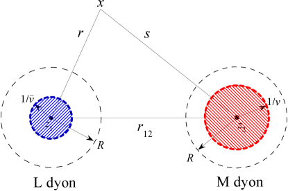
Figure 2: Three regions of integration for well separated dyons.

Although there is no principle difficulty in doing all calculations exactly for the whole caloron moduli space, at the stage of spatial integration of the determinant density we loose the capacity of performing analytical calculations for the simple reason that the expressions become too long, and so far we have not been able to put them into a manageable form in the general case. Therefore, we have to adopt a more subtle attitude. First of all we restrict ourselves to the part of the moduli space corresponding to large separations between dyons ($r_{12}\gg 1$). Physically, it seems to be the most interesting case. Furthermore, at the first stage we take $r_{12}{\rm v},r_{12}\overline{{\rm v}}\gg 1$, meaning that the dyons are well separated and do not overlap since the separation is then much bigger than the core sizes, see Fig. 1 (left). In this case, the vacuum current $J_{\mu}$ (16) becomes that of single dyons inside the spheres of some radius $R$ surrounding the dyon centers, such that $\frac{1}{{\rm v}},\frac{1}{\overline{{\rm v}}}\ll R\ll r_{12}$, and outside these spheres it can be computed analytically with the exponential precision, in accordance with subsection II.B, see Fig. 2. Adding up the contributions of the regions near two dyons and of the far-away region, we get $d{\rm Det}(-D^{2})/d{\rm v}$ for well-separated dyons. Integrating it over ${\rm v}$ we obtain the fermion determinant itself up to a constant and possible $1/r_{12}$ terms. Finally, we compute the $1/r_{12}$ corrections up to the $1/r_{12}^{5}$ term in the ${\rm Det}(-D^{2})$, which turn out to be quite non-trivial.

This is already an interesting result by itself, however, we would like to compute the constant, which can be done by matching our calculation with that for the trivial caloron at ${\rm v}=0$ and ${\rm v}=2\pi T$. It means that we have to extend the domain of applicability to $r_{12}{\rm v}={\cal O}(1)$ (or $r_{12}\overline{{\rm v}}={\cal O}(1)$) implying overlapping dyons, presented in Fig. 1 (right).

IV Near each of the dyons

In this section we calculate the right hand side of eq.(15) in the core domains of the L and M dyons. For M dyon this task is nearly solved in DGPS . In Appendix A the derivation of the vacuum current in the background is given and we have to multiply it by an expression for the gauge field (11) and integrate over M-dyon core domain (see Fig. 2). The result is

$${\rm tr}[\partial_{\rm v}A^{M}_{\mu}J^{M}_{\mu}]=\frac{{\left(1-s{\rm v}\coth(s{\rm v})\right)}^{3}\left(\sinh(2s{\rm v})-6s{\rm v}\right)}{96{\pi}^{2}s^{3}\sinh^{2}(s{\rm v})}-\frac{\left(1-s{\rm v}\coth(s{\rm v})\right)\left(\sinh(2s{\rm v})-2s{\rm v}\right)}{24s\sinh^{2}(s{\rm v})}$$ (22)

and integrating over the ball of radius $R$ surrounding the dyon we obtain

$$\int_{0}^{R}{\rm tr}[\partial_{\rm v}A^{M}_{\mu}J^{M}_{\mu}]d^{4}x=\frac{\pi}{432}+\frac{\gamma_{E}}{12\pi}+\frac{31}{144\pi}+\frac{\log({\rm v}/\pi)}{12\pi}-\int^{R}\partial_{\rm v}P\left[\frac{1}{2}\left(\overline{{\rm v}}+\frac{1}{s}\right)\right]4\pi s^{2}ds\;,$$ (23)

where we denote $P({\rm v})\equiv\frac{{\rm v}^{2}\overline{{\rm v}}^{2}}{12\pi^{2}}$ (in fact this function is a one-loop perturbative effective potential GPY ; NW ) and thus

$$-\int^{R}\partial_{\rm v}P\left[\frac{1}{2}\left(\overline{{\rm v}}+\frac{1}{s}\right)\right]s^{2}ds=\frac{R^{3}}{6}P^{\prime}\left(\frac{\overline{{\rm v}}}{2}\right)+\frac{R^{2}}{8}P^{\prime\prime}\left(\frac{\overline{{\rm v}}}{2}\right)+\frac{R}{16}P^{\prime\prime\prime}\left(\frac{\overline{{\rm v}}}{2}\right)+\frac{\log R}{96}P^{IV}\left(\frac{\overline{{\rm v}}}{2}\right)$$ (24)

The calculation in the L-dyon background is similar but slightly more difficult. The strategy is to reduce this problem to the calculation in the M-dyon background, which is simpler. For this purpose we note that the L-dyon gauge field is a gauge transformation of the M-dyon gauge field with the parameter ${\rm v}$ taken to be equal to $\overline{{\rm v}}=2\pi-{\rm v}$. We should note, however, that this transformation is anti-periodical in time and the anti-periodical Green function becomes a periodical one under this gauge transformation. It means that we have to the use the periodical vacuum current in the M-dyon background computed in the Appendix A and substitute ${\rm v}$ with $\overline{{\rm v}}$ to get the right answer:

$${\rm tr}[\partial_{\rm v}A^{L}_{\mu}J^{L}_{\mu}] = \frac{(r\overline{{\rm v}}\coth(r\overline{{\rm v}})-1)(\sinh(2r\overline{{\rm v}})-2r\overline{{\rm v}})}{12r\sinh^{2}(r\overline{{\rm v}})}+\frac{(r\overline{{\rm v}}\coth(r\overline{{\rm v}})-1)^{3}(\sinh(2r\overline{{\rm v}})-6r\overline{{\rm v}})}{96\pi^{2}r^{3}\sinh^{2}(r\overline{{\rm v}})}$$

$$- \frac{r\overline{{\rm v}}\coth(r\overline{{\rm v}})-1}{\coth\left(\frac{r\overline{{\rm v}}}{2}\right)}\;\frac{r\overline{{\rm v}}[2\cosh(r\overline{{\rm v}})+\cosh(2r\overline{{\rm v}})-4r\overline{{\rm v}}\coth\left(\frac{r\overline{{\rm v}}}{2}\right)+7]-\sinh(2{\rm r}\overline{{\rm v}})}{32\pi r^{2}\sinh^{2}(r\overline{{\rm v}})}.$$

Integration leads to the following result

$$\int_{0}^{R}{\rm tr}[\partial_{\rm v}A^{L}_{\mu}J^{L}_{\mu}]d^{4}x=-\frac{\pi}{432}-\frac{\gamma_{E}}{12\pi}-\frac{31}{144\pi}-\frac{\log(\overline{{\rm v}}/\pi)}{12\pi}-\int^{R}\partial_{\rm v}P\left[\frac{1}{2}\left(\overline{{\rm v}}-\frac{1}{r}\right)\right]4\pi r^{2}dr.$$ (26)

Finally, substituting (23) and (26) into (15) we arrive at the contribution from the cores

$$\left.\partial_{\rm v}\log{\rm Det}(-\nabla^{2})\right|_{\rm cores}=\frac{\log(\overline{{\rm v}}/{\rm v})}{12\pi}-\frac{4\pi R^{3}}{3}P^{\prime}\left(\frac{\overline{{\rm v}}}{2}\right)-\frac{\pi R}{2}P^{\prime\prime\prime}\left(\frac{\overline{{\rm v}}}{2}\right)\,.$$ (27)

V Contribution from the far region

In this region we can drop the exponentially small terms $e^{-{\rm v}s}$ and $e^{-\overline{{\rm v}}r}$ in the r.h.s. of eq.(15). It turns out to be a great simplification. The calculations are similarly to the calculations for isospin-1 DGPS . We are not repeating them here because the result is simple and natural. The full vacuum current can be easily expressed through the perturbative potential energy $P({\rm v})\equiv\frac{{\rm v}^{2}\overline{{\rm v}}^{2}}{12\pi^{2}}$. The only non-zero component is

$$J_{4}=-\frac{i\tau_{3}}{2}\left.P^{\prime}(q)\right|_{q=\frac{1}{2}\left(\overline{{\rm v}}+\frac{1}{s}-\frac{1}{r}\right)}\,.$$ (28)

Making use of eq.(13) we come to the contribution from the far region

$$\left.\partial_{\rm v}\log{\rm Det}(-\nabla^{2})\right|_{\rm far}=\int\partial_{{\rm v}}P\left[\frac{1}{2}\left(\overline{{\rm v}}+\frac{1}{s}-\frac{1}{r}\right)\right]d^{4}x$$ (29)

The integral is taken over the whole space with two holes (see Fig. 2). We can use the symmetry between dyons to write

$$\int\partial_{{\rm v}}P\left[\frac{1}{2}\left(\overline{{\rm v}}+\frac{1}{s}-\frac{1}{r}\right)\right]d^{4}x=-\frac{1}{2}P^{\prime}\left(\frac{\overline{{\rm v}}}{2}\right)\left(V-2\frac{4\pi}{3}R^{3}\right)-\frac{1}{16}P^{\prime\prime\prime}\left(\frac{\overline{{\rm v}}}{2}\right)(4\pi r_{12}-8\pi R)+{\cal O}\left(\frac{\log R}{R}\right)$$ (30)

where $V$ is the 3D volume of the system.

VI Combining all three regions

Adding (30) to (27) we get the expression for the ${\rm v}$ derivative of the determinant for large distances $r_{12}$ between constituents with the $1/r_{12}$ precision:

$$\partial_{\rm v}\log{\rm Det}(-\nabla^{2})=-\frac{\log({\rm v}/\overline{{\rm v}})}{12\pi}-\frac{1}{2}P^{\prime}\left(\frac{\overline{{\rm v}}}{2}\right)V-\frac{1}{16}P^{\prime\prime\prime}\left(\frac{\overline{{\rm v}}}{2}\right)4\pi r_{12}$$ (31)

This equation can be easily integrated over ${\rm v}$ up to a constant, which in fact can be a function of the separation $r_{12}$:

$$\left.\log{\rm Det}(-\nabla^{2})\right|_{\rm far}=\left[P\left(\frac{\overline{{\rm v}}}{2}\right)-\frac{\pi^{2}}{12}\right]V+P^{\prime\prime}\left(\frac{\overline{{\rm v}}}{2}\right)\frac{\pi r_{12}}{2}-\frac{\overline{{\rm v}}\log{\overline{{\rm v}}}}{12\pi}-\frac{{\rm v}\log{{\rm v}}}{12\pi}+f(r_{12})$$ (32)

This result is valid with ${\cal O}(\exp(-{\rm v}r_{12}),\exp(-\overline{{\rm v}}r_{12}),1/r_{12})$ precision, and we have separated a constant $\frac{\pi^{2}}{12}=P(\pi),$ which accounts for normalization to the ${\rm v}=0$ determinant. Since in the above calculation of the determinant for well-separated dyons we have neglected the Coulomb field of one dyon inside the core region of the other, we expect that the unknown function $f(r_{12})={\cal O}(1/r_{12})+c_{\frac{1}{2}}$ where $c_{\frac{1}{2}}$ is the true integration constant. One should consider the $r_{12}$-derivative of the determinant to see this explicitly. We perform it in Section VIII. Our next aim will be to find the constant $c_{\frac{1}{2}}$. The ${\cal O}(1/r_{12})$ corrections will be found later.

VII Expression for the constant in the determinant

To find the integration constant, one needs to know the value of the determinant at ${\rm v}\!=\!0$, where the KvBLL caloron with non-trivial holonomy reduces to the Harrington–Shepard caloron with trivial holonomy, and for which the determinant has been computed by Gross, Pisarski and Yaffe (GPY) GPY . Before we match our determinant at ${\rm v}\!\neq\!0$ with that at ${\rm v}\!=\!0$, let us recall the GPY result for the isospin-1/2 determinant.

VII.1 Det${\bf(-\nabla^{2})}$ at ${\rm v}=0$

The ${\rm v}\!=\!0,\;2\pi$, periodic instanton is traditionally parameterized by the instanton size $\rho$. It is known Rossi ; GPY that the periodic instanton can be viewed as composed of two BPS monopoles one of which has an infinite size. It becomes especially clear in the KvBLL construction KvB ; LL , where the size of the M (L) dyon becomes infinite as ${\rm v}\to 0\;(2\pi)$, see section II. Despite one dyon being infinitely large, one can still continue to parameterize the caloron by the distance $r_{12}$ between dyon centers, with $\rho=\sqrt{r_{12}/\pi}$. Since the determinant (32) is given in terms of $r_{12}$ we have first of all to rewrite the GPY determinant in terms of $r_{12}$, too. Actually, GPY have interpolated the determinant in the whole range of $\rho$ (hence $r_{12}$) but we shall be interested only in the limit $r_{12}\gg 1$. In this range the GPY result reads:

$$\log{\rm Det}(-\nabla^{2})=\left.\log{\rm Det}(-\nabla^{2})\right|_{{\rm v},T=0}+\eta\frac{\pi r_{12}}{3}-\frac{1}{12}\log r_{12}+\frac{c_{0}}{16}+{\cal O}\left(\frac{1}{r_{12}}\right)$$ (33)

where $\eta=-1/2$ for anti-periodic boundary conditions (i.e. ${\rm v}=0$, and M-dyon is infinitely large), $\eta=1$ for periodic conditions (i.e. ${\rm v}=2\pi$, and L-dyon is large). One can verify that the term linear in $d$ in this expression is exactly equal to the term linear in $d$ in eq.(32) when ${\rm v}=0$ for anti-periodic and when ${\rm v}=2\pi$ for periodic boundary conditions. In Ref. DGPS we have managed to find a constant $c_{0}$ analytically:

$$c_{0}=\frac{8}{9}-\frac{8\,\gamma_{E}}{3}-\frac{2\,\pi^{2}}{27}+\frac{4\,\log\pi}{3}$$

The zero-temperature instanton determinant is tHooft :

$$\left.\log{\rm Det}(-\nabla^{2})\right|_{{\rm v},T=0} = \frac{1}{6}\log\mu+\frac{1}{12}\log\left(\frac{r_{12}}{\pi}\right)+\alpha(1/2)\;,$$ (34)

where it is implied that the determinant is regularized by the Pauli–Villars method and $\mu$ is the Pauli–Villars mass. Thus the isospin-1/2 result for the case of trivial holonomy is

$$\log{\rm Det}(-\nabla^{2})=\eta\frac{\pi r_{12}}{3}+\frac{c_{0}}{16}+\alpha(1/2)-\frac{1}{12}\log\pi+\frac{1}{6}\log\mu\;,$$ (35)

where

$$\alpha(1/2)=-\frac{17}{72}+\frac{\gamma_{E}}{6}+\frac{\log\pi}{6}-\frac{\zeta^{\prime}(2)}{\pi^{2}}$$ (36)

We have to match our eq.(32) with eq.(35) at ${\rm v}=0$ or ${\rm v}=2\pi$, but eq.(32) has been derived assuming $r_{12}\gg\frac{1}{{\rm v}},\frac{1}{\overline{{\rm v}}}$ and one cannot formally take the limit ${\rm v}\to 0$ in that expression without taking simultaneously $r_{12}\to\infty$. In the next subsection we will show that one can actually take this limit and get a correct constant. We will rely on exact results to show that eq.(32) is valid for arbitrary values of ${\rm v}r_{12}$ and $\overline{{\rm v}}r_{12}$ (but large $r_{12}\gg 1$).

VII.2 Extending the result to arbitrary values of ${\rm v}r_{12}$

Let us take a fixed but large value of the dyon separation $r_{12}\gg 1$ such that both eq.(32) and eq.(35) are valid. Actually, our aim is to integrate the exact expression for the derivative of the determinant

$$\partial_{\rm v}\log{\rm Det}(-\nabla^{2})=\int\wp(x)d^{4}x,\qquad\wp(x)\equiv-{\rm Tr}\left[\partial_{\rm v}A_{\mu}J^{\mu}\right],$$ (37)

from ${\rm v}=0$, where the determinant is given by eq.(35), to some small value of ${\rm v}\ll 1$ (but such that ${\rm v}r_{12}\gg 1$), where eq.(32) becomes valid. We shall parameterize this ${\rm v}$ as ${\rm v}=k/r_{12}\ll 1$ with $k\gg 1$. The result of the integration over ${\rm v}$ must be equal to the difference between the right hand sides of eqs.(32,35). We want to show that it is ${\cal O}(k/r_{12})$; it means that there are no large corrections to eq.(32) at small ${\rm v}$ that can alter the constant term in the determinant. Denoting by $\bar{\wp}$ our $\wp$ with subtracted asymptotic terms we have to show that

$$\int_{0}^{\frac{k}{r_{12}}}d{\rm v}\int\!d^{4}x\,\bar{\wp}(x)={\cal O}\left(\frac{1}{r_{12}}\right)\;.$$ (38)

In this integration we are in the domain $1/{\rm v}\gg 1$ and $r_{12}\gg 1$ and we can simplify the integrand dropping terms which are small in this domain. At this point it will be convenient to restore temporarily the temperature dependence. With $\beta\equiv 1/T$ our domain of interest is $1/{\rm v}\gg\beta$ and $r_{12}\gg\beta$. Therefore we are in the small-$\beta$ range and can expand $\bar{\wp}$ in series with respect to $\beta$:

$$\bar{\wp}=\frac{1}{\beta^{2}}\wp_{0}+\frac{1}{\beta}\wp_{1}+{\cal O}(\beta^{0})\;.$$ (39)

As we shall see in a moment, only the first two terms can be not small in this range and we need to know only them to compute $c_{2}$. It is a great simplification because $\wp_{0,1}$ does not contain terms proportional to $e^{-\overline{{\rm v}}r}$ since $\overline{{\rm v}}=2\pi T-{\rm v}\to\infty$ at $\beta\to 0$, and what is left is time independent. Moreover, what is left after we neglect exponentially small terms are homogeneous functions of $r,s,r_{12},{\rm v}$ and we can turn to the dimensionless variables:

$$\wp_{0}(r,s,r_{12},{\rm v})=\frac{1}{r_{12}}\widetilde{\wp}_{0}\left(\frac{r}{r_{12}},\frac{s}{r_{12}},{\rm v}r_{12}\right)\;.$$ (40)

From the exact expressions we see that $\wp_{1}\equiv 0$. The reason is that there is no $1/\beta$ term in eq.(67). Actually the same phenomenon can be seen for the single dyon in eq.(22). We rewrite the l.h.s. of eq.(38) in terms of the new variables:

$$\int\!d^{4}x\,\bar{\wp}(x)=\frac{r_{12}^{2}}{\beta}\int\!d^{3}\tilde{x}\,\widetilde{\wp}_{0}+{\cal O}(\beta)=\frac{r_{12}^{2}}{\beta}F_{0}({\rm v}r_{12})+{\cal O}(\beta)\;,$$ (41)

where $\tilde{x}=x/r_{12}$ is dimensionless. We see that it is indeed sufficient to take just the first two terms in the expansion (39) at $\beta\to 0$.

Let us try to integrate eq.(41) over ${\rm v}$ from 0 to $k/r_{12}$ even without explicit knowledge of $F_{0}$. We get

$$\int\limits_{0}^{k/r_{12}}\frac{r_{12}^{2}}{\beta}F_{0}({\rm v}r_{12})d{\rm v}=\frac{r_{12}}{\beta}\int\limits_{0}^{k}F_{0}({\rm v}r_{12})d({\rm v}r_{12})$$ (42)

We know that the approximate result eq.(32) is correct with at least ${\cal O}(\exp(-k),1/({\rm v}r_{12}))$ precision, so at large $k$ the correction to eq.(32) must be a constant, plus a term of the order of $1/({\rm v}r_{12})=1/k$. Therefore, $F_{0}$ must be zero. We have checked numerically that it is indeed so (actually this function $F_{0}$ is the same as in DGPS ).

Thus, we have proved eq.(38). We can now compare eq.(32) with eq.(35) and get the constant:

$$c_{\frac{1}{2}}=\frac{c_{0}}{16}+\alpha(1/2)+\frac{1}{12}\log 4\pi+\frac{1}{6}\log\mu=\frac{1}{6}\log\mu+\frac{36\log(2\pi^{2})-39-\pi^{2}}{216}-\frac{\zeta^{\prime}(2)}{\pi^{2}}=\frac{1}{6}\log\mu+0.36584648$$ (43)

It means that eq.(32) is right in whole range $0\leq{\rm v}\leq 2\pi$ with the accuracy $1/r_{12}$.

VIII $1/r_{12}$ corrections

In the previous section we have seen that Eq.(32) is valid to all orders in $1/({\rm v}r_{12}),1/(\overline{{\rm v}}r_{12})$; however, there are other $1/r_{12}$ corrections which are not accompanied by the $1/{\rm v},\;1/\overline{{\rm v}}$ factors: the aim of this subsection is to find them using the exact vacuum current.

To this end, we again consider the case $r_{12}\gg\frac{1}{{\rm v}},\,\frac{1}{\overline{{\rm v}}}$ such that one can split the integration over $3d$ space into three domains shown in Fig. 2. In the far-away domain one can use the same vacuum current as we had in Section V, as it has an exponential precision with respect to the distances to both dyons. In the core regions, however, it is now insufficient to neglect completely the field of the other dyon, as we did in Section IV looking for the leading order. Since we are now after the $1/r_{12}$ corrections, we have to use the exact field and the exact vacuum current of the caloron but we can neglect the exponentially small terms of order $e^{-r_{12}}$.

Another modification with respect to section IV is that we find it more useful this time to choose $r_{12}$ as the parameter $\cal P$ in eq.(15). We shall compute the $1/r_{12}^{2}$ and higher terms in $\partial{\rm Det}(\!-\!D^{2})/\partial r_{12}$ and then restore the determinant itself since the limit of $r_{12}\to\infty$ is already known. Let us define how the KvBLL field depends on $r_{12}$. As is seen from eq.(7) the KvBLL field is a function of $r,\;s,\;{\rm v},\;r_{12}$ only. We define the change in the separation $r_{12}\to r_{12}+dr_{12}$ as the symmetric displacement of each monopole center by $\pm dr_{12}/2$. It corresponds to

$$\frac{\partial r}{\partial r_{12}}=\frac{r_{12}^{2}+r^{2}-s^{2}}{4r_{12}r},\qquad\frac{\partial s}{\partial r_{12}}=\frac{r_{12}^{2}+s^{2}-r^{2}}{4r_{12}s}.$$ (44)

We shall use the definition (44) to compute the derivative of the caloron field (4) with respect to $r_{12}$.

Let us start from the $M$-monopole core region. To get the $1/r_{12}$ correction to the determinant we need to compute its derivative in the $1/r_{12}^{2}$ order and expand correspondingly the caloron field and the vacuum current to this order. Wherever the distance $r$ from the far-away L dyon appears in the equations, we replace it by $r=(r_{12}^{2}+2sr_{12}\cos\theta+s^{2})^{1/2}$, where $s$ is the distance from the M-dyon and $\theta$ is the polar angle seen from the M-dyon center. Expanding in inverse powers of $r_{12}$ we get the coefficients that are functions of $s,\cos\theta$. One can easily integrate over $\theta$ as the integration measure in spherical coordinates is $2\pi s^{2}ds\;d\cos\theta$. Then we integrate over $s$, the distance to the core of the M-monopole. After that we have to add contributions from the L and M dyon cores and from the far-away domain. It turns out that contributions from dyons differ by terms dependent on $R$ only:

$$\partial_{r_{12}}\log{\rm Det}_{\rm core} = \frac{1}{r_{12}^{2}}\left(\frac{23}{72\pi}+\frac{\gamma}{6\pi}+\frac{\pi}{216}+\frac{\log(R^{2}{\rm v}\overline{{\rm v}}/\pi^{2})}{12\pi}\right)+\frac{1}{12r_{12}^{3}\pi}\left(\frac{1}{{\rm v}}+\frac{1}{\overline{{\rm v}}}\right)$$

$$- \frac{1}{24r_{12}^{4}\pi}\left(\frac{1}{{\rm v}^{2}}+\frac{1}{\overline{{\rm v}}^{2}}\right)+\frac{60-\pi^{4}}{2160r_{12}^{5}\pi}\left(\frac{1}{{\rm v}^{3}}+\frac{1}{\overline{{\rm v}}^{3}}\right)+{\cal O}\left(\frac{1}{r_{12}^{6}}\right)$$

(we drop here powers of $R$ as they cancel with the contribution from the far domain)

Now let us turn to the far-away domain. Recalling eq.(28) we realize that the contribution of this region is determined by the potential energy:

$$\left.\frac{\partial\log{\rm Det}(\!-\!\nabla^{2})}{\partial r_{12}}\right|_{\rm far} = \int\!d^{3}x\,\partial_{r_{12}}P\left(\frac{1}{2}\left[\overline{{\rm v}}-\frac{1}{r}+\frac{1}{s}\right]\right)$$

$$= \frac{1}{8}P^{\prime\prime}(\overline{{\rm v}}/2)\int\!d^{3}x\,\partial_{r_{12}}\left(\frac{1}{r}-\frac{1}{s}\right)^{2}+\frac{1}{384}P^{\rm IV}(\overline{{\rm v}}/2)\int\!d^{3}x\,\partial_{r_{12}}\left(\frac{1}{r}-\frac{1}{s}\right)^{4}.$$

The integration range is the $3d$ volume with two balls of radius $R$ removed. We use

$$\int\partial_{r_{12}}\left(\frac{1}{r}-\frac{1}{s}\right)^{2}d^{3}x = 4\pi-\frac{16\pi R^{2}}{3r_{12}^{2}}+\sum_{n=1}^{\infty}\frac{8n\pi}{(2n-1)(2n+1)}\left(\frac{R}{r_{12}}\right)^{2n+1}$$ (47)

$$\int\partial_{r_{12}}\left(\frac{1}{r}-\frac{1}{s}\right)^{4}d^{3}x = \frac{32\pi\log(r_{12}/R)}{r_{12}^{2}}+\frac{2\pi(8-9\pi^{2})}{3r_{12}^{2}}+\frac{80\pi R}{r_{12}^{3}}-\frac{32\pi R^{2}}{r_{12}^{4}}+\frac{304\pi R^{3}}{15r_{12}^{5}}+{\cal O}(1/r_{12}^{6})$$

Adding up all three contributions we see that the region separation radius $R$ gets canceled (as it should), and we come to:

$$\partial_{r_{12}}\log{\rm Det}(-\nabla^{2}) = \frac{\pi}{2}P^{\prime\prime}\left(\frac{\overline{{\rm v}}}{2}\right)+\frac{1}{12r_{12}^{2}\pi}\left(\log({\rm v}\overline{{\rm v}}r_{12}^{2}/\pi^{2})-\frac{23\pi^{2}}{72}+2\gamma+\frac{25}{6}\right)$$

$$+ \frac{1}{12r_{12}^{3}\pi}\left(\frac{1}{{\rm v}}+\frac{1}{\overline{{\rm v}}}\right)-\frac{1}{24r_{12}^{4}\pi}\left(\frac{1}{{\rm v}^{2}}+\frac{1}{\overline{{\rm v}}^{2}}\right)+\frac{60-\pi^{4}}{2160r_{12}^{5}\pi}\left(\frac{1}{{\rm v}^{3}}+\frac{1}{\overline{{\rm v}}^{3}}\right)+{\cal O}\left(\frac{1}{r_{12}^{6}}\right)\;.$$

Integrating over $r_{12}$ gives

$$\log{\rm Det}(-\nabla^{2}) = \frac{\pi}{2}P^{\prime\prime}\left(\frac{\overline{{\rm v}}}{2}\right)r_{12}-\frac{1}{12r_{12}\pi}\left(\log({\rm v}\overline{{\rm v}}r_{12}^{2}/\pi^{2})-\frac{23\pi^{2}}{72}+2\gamma+\frac{37}{6}\right)-\frac{1}{24r_{12}^{2}\pi}\left(\frac{1}{{\rm v}}+\frac{1}{\overline{{\rm v}}}\right)$$

$$+ \frac{1}{72r_{12}^{3}\pi}\left(\frac{1}{{\rm v}^{2}}+\frac{1}{\overline{{\rm v}}^{2}}\right)-\frac{60-\pi^{4}}{8640r_{12}^{4}\pi}\left(\frac{1}{{\rm v}^{3}}+\frac{1}{\overline{{\rm v}}^{3}}\right)+\frac{12-\pi^{4}}{2880r_{12}^{5}\pi}\left(\frac{1}{{\rm v}^{4}}+\frac{1}{\overline{{\rm v}}^{4}}\right)+\bar{c}+{\cal O}\left(\frac{1}{r_{12}^{6}}\right)\;,$$

where $\bar{c}$ is the integration constant that does not depend on $r_{12}$. Comparing eq.(VIII) with eq.(32) at $r_{12}\to\infty$ we conclude that

$$\bar{c}=V\,\left[P\left(\frac{\overline{{\rm v}}}{2}\right)-\frac{\pi^{2}}{12}\right]-\frac{\overline{{\rm v}}\log{\overline{{\rm v}}}}{12\pi}-\frac{{\rm v}\log{{\rm v}}}{12\pi}+c_{\frac{1}{2}}$$ (50)

and $c_{\frac{1}{2}}$ is given in eq.(43). We note that the leading correction, $\log r_{12}/r_{12}$, arises from the far-away range and is related to the potential energy, similar to the leading $r_{12}$ term. This series in $1/r_{12}$ is asymptotic as the coefficients are rapidly increasing.

Interesting, we have revealed that the contribution from the regular part of the current $J^{\rm r}$ has no corrections $1/r_{12}^{n}$ (we verified that up to the $10^{\rm th}$ order) and is determined completely by the far asymptote

$$\!-\!\int d^{4}x\,{\rm Tr}\left(\partial_{r_{12}}A_{\mu}\,J^{\rm r}_{\mu}\right)\simeq P^{\prime\prime}\left(\frac{\overline{{\rm v}}}{2}\right)\frac{\pi}{2}\;.$$ (51)

It seems that ${\rm Tr}\left(\partial_{r_{12}}A_{\mu}\,J^{\rm r}_{\mu}\right)$ is a full derivative of a simple expression.

IX Asymptote of small separation

In this domain of the moduli space of the KvBLL caloron it is important to realize that KvBLL caloron is a chain of the usual BPST instantons equally separated in time direction with a fixed relative gauge orientation between the neighbors.

When the size of instantons is large compared to their separation $1/T$, they overlap and cannot be thought of as individual pseudoparticles. It is much simpler to consider the KvBLL caloron as a bound state of two BPS dyons. Small separations correspond to the small instanton size $\rho$ since $\rho=\sqrt{r_{12}/\pi}$. It means that instantons do not overlap, and the KvBLL caloron reduces to the usual BPST caloron.

Formally, one switches to dimensionless variables $r=\bar{r}\rho,\;s=\bar{s}\rho$ and then takes the limit $\rho\rightarrow 0$. In this limit the gauge field of the KvBLL caloron becomes that of the ordinary instanton of vanishing size, plus a constant field. It is then clear that the determinant becomes that of the ordinary instanton, plus a contribution from a constant field:

$$\log{\rm Det}(-\nabla^{2})=\left[P\left(\frac{\overline{{\rm v}}}{2}\right)-\frac{\pi^{2}}{12}\right]V+\frac{1}{6}\log\mu+\frac{1}{12}\log\left(\frac{r_{12}}{\pi}\right)+\alpha(1/2)+{\cal O}(\rho)\;,\;\;\;\;\;\alpha(1/2)=0.145873$$ (52)

One can expand in powers of $\rho$ further, but it requires knowledge of the exact expression for the vacuum current (16). Here we give only the final result. The contribution from the regular part of the current $J^{\rm r}$ for small $r_{12}$ is

$$\!-\!\int d^{4}x\,{\rm Tr}\left(\partial_{r_{12}}A_{\mu}\,J^{\rm r}_{\mu}\right)=P^{\prime\prime}\left(\frac{\overline{{\rm v}}}{2}\right)\frac{\pi}{2}+{\cal O}(\rho)$$ (53)

and from the singular part

$$\!-\!\int d^{4}x\,{\rm Tr}\left(\partial_{r_{12}}A_{\mu}\,J^{\rm s}_{\mu}\right)=\frac{1}{12\pi\rho^{2}}+(3{\rm v}\overline{{\rm v}}-2\pi^{2})\frac{1}{72\pi}+{\cal O}(\rho)$$ (54)

taking into account these contributions we have

$$\log{\rm Det}(-\nabla^{2})=\left[P\left(\frac{\overline{{\rm v}}}{2}\right)-\frac{\pi^{2}}{12}\right]V+\alpha(1/2)+\frac{1}{6}\log(\mu\rho)-(7\pi^{2}-3\pi{\rm v}-3{\rm v}^{2})\frac{\rho^{2}}{36}+{\cal O}(\rho^{3})\;,$$ (55)

Note that the contribution from the regular part of the vacuum current for small values of $r_{12}$ is exactly the same as it has been for large $r_{12}$ in eq.(51). It suggests that eq.(51) is exact. Unfortunately, we have not been able to prove it analytically, but we have verified it numerically. We have found out that eq.(51) is correct for all $r_{12}$ and ${\rm v}$ with the precision of at least $10^{-3}$.

X Numerical evaluation

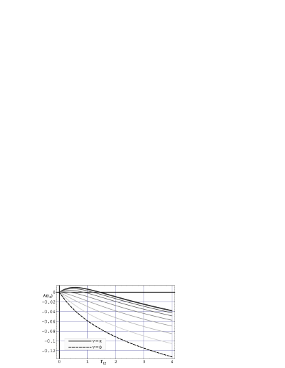
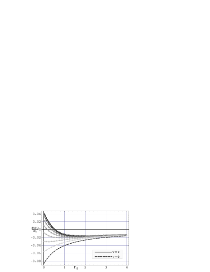
Figure 3: Result of the numerical evaluation of $A({\rm v},r_{12})$. The dashed line corresponds to the trivial holonomy (left). Fist, we have computed $\partial_{r_{12}}A({\rm v},r_{12})$ (right), and then integrated it from $r_{12}=\infty$ to $r_{12}=0$. All the curves on the left plot go to zero as $r_{12}\rightarrow 0$ with an accuracy $10^{-4}$; that proves the consistency of our small $r_{12}$ and large $r_{12}$ asymptotics.

One can hardly expect a compact analytical expression for the determinant at arbitrary separations (or instanton sizes) and holonomies as even for the case of the trivial holonomy, studied by Gross, Pisarski and Yaffe GPY , it is not known. In this section we present our results of the numerical evaluation of the determinant for arbitrary separations and holonomies.

We start from eq.(15) and calculate the exact analytical expression for the vacuum current (16) using (19) and the exact expression from DGPS for the ADHM construction. The resulting expression is too lengthy for printing but can be provided by request. We calculate the trace in the integrand in the r.h.s. of eq.(15) with a particular choice of the parameter $\cal P$.

We have taken ${\cal P}=r_{12}$. Using the axial symmetry we can reduce the number of integrations to 3. We have managed to perform the integration numerically with the precision $10^{-4}$, despite the complexity of the expression. The numerical data are shown in Fig. 3. One can see that it is consistent with all our analytical results. Following GPY we denote

$$\log{\rm Det}(-\nabla^{2})=\left.\log{\rm Det}(-\nabla^{2})\right|_{{\rm v},T=0}+A({\rm v},r_{12})+\left[P\left(\frac{\overline{{\rm v}}}{2}\right)-\frac{\pi^{2}}{12}\right]V+P^{\prime\prime}\left(\frac{\overline{{\rm v}}}{2}\right)\frac{\pi r_{12}}{2}\,,$$ (56)

where $\left.\log{\rm Det}(-\nabla^{2})\right|_{{\rm v},T=0}$ is given in eq.(34). Note that if eq.(51) is exact, only the singular part of the current $J^{\rm s}$ contributes to $A({\rm v},r_{12})$, thus $A({\rm v},r_{12})$ must be symmetric under the exchange ${\rm v}\leftrightarrow\overline{{\rm v}}$. We have verified this symmetry numerically. From (VIII,54) we see that $A({\rm v},r_{12})$ has the following asymptotics (valid for all ${\rm v}$)

$$A({\rm v},r_{12})=\frac{\log(2\pi)}{6}-\frac{{\rm v}\log{\rm v}}{12\pi}-\frac{\overline{{\rm v}}\log\overline{{\rm v}}}{12\pi}+\frac{1}{18}-\frac{\gamma}{6}-\frac{\pi^{2}}{216}-\frac{\log(r_{12}/\pi)}{12}+{\cal O}\left(\frac{1}{r_{12}}\right)=\frac{(3{\rm v}\overline{{\rm v}}-2\pi^{2})r_{12}}{72\pi}+{\cal O}\left(r_{12}^{3/2}\right)$$ (57)

We find that $A({\rm v},r_{12})$ can be fitted by the following expression

$$A({\rm v},r_{12})\simeq-\frac{1}{12}\log\left(1+\frac{\pi r_{12}}{3}\right)-\frac{r_{12}\alpha}{216\pi(1+r_{12})}+\frac{0.00302\;r_{12}(\alpha+9{\rm v}\overline{{\rm v}})}{2.0488+r_{12}^{2}}$$ (58)

where $\alpha=18{\rm v}\log{\rm v}+18\overline{{\rm v}}\log\overline{{\rm v}}-216.611$. This expression has a maximum absolute error $5\times 10^{-3}$.

XI Summary

In this paper we have considered finite temperature QCD with light fundamental fermions and calculated the fermionic contribution to the 1-loop quantum weight of the instanton with non-trivial value of holonomy (or Polyakov line) at spatial infinity.

Finite temperature theory is formulated in terms of the Euclidean QCD partition function with (anti-)periodic boundary conditions in time with the period $\beta=1/T$, where $T$ is the temperature.

The instanton with non-trivial holonomy (or the KvBLL caloron KvB ; LL for brevity) is the most general self-dual solution of the YM equations of motion with a unit topological charge and the above-mentioned periodicity conditions imposed. The solution is parameterized by the holonomy ${\rm v}$ at spatial infinity, the temperature $T=1/\beta$, the size $r_{12}$, center position, and color orientation. When $r_{12}\ll\beta$ the solution reduces to the ordinary BPST instanton with size $\rho=\sqrt{r_{12}T/\pi}$ in the domain $x_{\mu}^{2}\sim\rho^{2}$ which gives the main contribution to the action density. In the opposite limit $r_{12}\gg\beta$ it can be described as a superposition of two (for $N_{c}=2$) properly gauge-combed BPS monopoles with the separation $r_{12}$ between them.

One can assume that the effective gauge coupling is reasonably small at the deconfinement and chiral symmetry restoration temperatures and that therefore the semiclassical ensemble of the KvBLL calorons makes sense and can be relevant for describing those phase transitions. It is therefore important to calculate the quantum weight of an individual KvBLL caloron as the first step in the study of the ensemble of calorons. The gluonic contribution to the quantum weight has been calculated in Ref. DGPS . In this paper we have extended the methods and the result of that work to the theory with light fermions – by computing the fermionic determinant over non-zero modes ${\rm Det}^{\prime}(i\nabla/\hskip 3.00003pt)$. The zero fermion modes Cherndb should be taken separately when constructing the ensemble, in the spirit of Ref. DP2a ; DP2b ; it will be considered elsewhere.

The main result of the paper is the determinant in the fundamental representation in the background field of the KvBLL caloron (7):

$$\frac{1}{2}\log{\rm Det}^{\prime}(i\nabla/\hskip 3.00003pt(A^{P}))=\left.\log{\rm Det}(-\nabla^{2})\right|_{{\rm v},T=0}+A({\rm v}/T,r_{12}T)+\left[P\left(\frac{\overline{{\rm v}}}{2}\right)-\frac{\pi^{2}}{12}T^{3}\right]V+P^{\prime\prime}\left(\frac{\overline{{\rm v}}}{2}\right)\frac{\pi r_{12}}{2}\,,$$ (59)

where $V$ is a $3d$ volume and $\overline{{\rm v}}=2\pi T-{\rm v}$.

Since the fundamental representation is sensitive to the sign of the asymptotic holonomy $e^{i{\rm v}T\tau_{3}/2}$, the fermionic determinant is $4\pi T$ periodic in ${\rm v}$, in contrast to the period of $2\pi T$ for the gluon and ghost determinants. We have also considered the background field (8) for which one has to exchange ${\rm v}$ with $\overline{{\rm v}}$ in eq.(59).

The numerical values of the quantity $A({\rm v},r_{12})$ are tabulated in Appendix B; they can be fitted by eq.(58) consistent with the asymptotic expansion of this quantity at large dyons’ separations,

$$A({\rm v},r_{12}) = \frac{\log(2\pi)}{6}-\frac{{\rm v}\log{\rm v}}{12\pi}-\frac{\overline{{\rm v}}\log\overline{{\rm v}}}{12\pi}+\frac{1}{18}-\frac{\gamma}{6}-\frac{\pi^{2}}{216}-\frac{\log(r_{12}/\pi)}{12}$$

$$-\frac{1}{12r_{12}\pi}\left(\log({\rm v}\overline{{\rm v}}r_{12}^{2}/\pi^{2})-\frac{23\pi^{2}}{72}+2\gamma+\frac{37}{6}\right)-\frac{1}{24r_{12}^{2}\pi}\left(\frac{1}{{\rm v}}+\frac{1}{\overline{{\rm v}}}\right)$$

$$+ \frac{1}{72r_{12}^{3}\pi}\left(\frac{1}{{\rm v}^{2}}+\frac{1}{\overline{{\rm v}}^{2}}\right)-\frac{60-\pi^{4}}{8640r_{12}^{4}\pi}\left(\frac{1}{{\rm v}^{3}}+\frac{1}{\overline{{\rm v}}^{3}}\right)+\frac{12-\pi^{4}}{2880r_{12}^{5}\pi}\left(\frac{1}{{\rm v}^{4}}+\frac{1}{\overline{{\rm v}}^{4}}\right)+{\cal O}\left(\frac{1}{r_{12}^{6}}\right)\;,$$

and with the expansion at small $r_{12}$ (see eq.(55)),

$$A({\rm v},r_{12})=\frac{r_{12}\left(3{\rm v}\overline{{\rm v}}-2\pi^{2}\right)}{72\pi}+{\cal O}(r_{12}^{3/2})$$ (61)

The generalization of these results to the case of larger groups, $N_{c}>2$, will be published elsewhere GSN .

Appendix A Derivation of the vacuum current in the BPS dyon background

Here we calculate the isospin-1/2 current (16) in the M-dyon background (11). In Section IV it has been explained that the calculation in the L-dyon background is equivalent to the calculation for the M-dyon, but with the periodical boundary conditions. To calculate the vacuum current, we use the expression for the ADHM quantity $|v{\rangle}$ for the M-dyon from the Appendix A of DGPS . It states

$$|v{\rangle}=e^{i\frac{\phi}{2}\tau^{3}}e^{-i\frac{\pi-\theta}{2}\tau_{2}}e^{i\frac{\phi}{2}\tau^{3}}\sqrt{\frac{{\rm v}s}{\sinh({\rm v}s)}}\exp[z{\rm v}(ix_{4}+s\tau^{3})]$$ (62)

We shall use the explicit expression for the Green function in the ADHM background (19).

A.1 Singular part of the dyon current $J^{\rm s}_{\mu}$

The regularized singular part of the current was in fact already computed in Appendix C of DGPS . It was named $j_{\mu}$ there. The result was

$$J^{\rm s}_{r} = 0,$$

$$J^{\rm s}_{\phi} = -\frac{i{\rm v}\left(s^{2}{\rm v}^{2}{\mathrm{csch}^{2}(s{\rm v})+s{\rm v}\coth(s{\rm v})-2}\right)}{48\pi^{2}s^{2}\sinh(s{\rm v})}(\cos(\phi)\,\tau_{1}+\sin(\phi)\,\tau_{2}),$$

$$J^{\rm s}_{\theta} = -\frac{i{\rm v}\left(s^{2}{\rm v}^{2}{\mathrm{csch}^{2}(s{\rm v})+s{\rm v}\coth(s{\rm v})-2}\right)}{48\pi^{2}s^{2}\sinh(s{\rm v})}(\sin(\phi)\,\tau_{1}-\cos(\phi)\,\tau_{2}),$$

$$J^{\rm s}_{4} = -\frac{i\left(\sinh^{2}(s{\rm v})-s^{3}{\rm v}^{3}\coth(s{\rm v})\right)}{48\pi^{2}s^{3}\sinh^{2}(s{\rm v})}\tau_{3}\;,$$ (63)

where $\tau$ are Pauli matrices, $s$, $\phi$ and $\theta$ are the spherical coordinates centered at the monopole position. Eq.(63) obviously does not depend on the temperature and the type of the boundary conditions as it is a purely zero-temperature object.

A.2 Regular part of the monopole current $J^{\rm r}_{\mu}$

We are going to calculate the part of the anti-periodical vacuum current corresponding to

$$({\cal G}^{{\rm r}})^{ab}(x,y)\equiv\sum_{n\neq 0}(-1)^{n}\frac{{\langle}v(x)|v(y_{n}){\rangle}}{4\pi^{2}(x-y_{n})^{2}},\qquad y_{n}=\vec{y},\quad y_{n4}=y_{4}+n,$$ (64)

This derivation is similar to that done for isospin-1 in DGPS . We repeat it here because it is more simple for the isospin-1/2 case owing to the simple form of the isospin-1/2 Green function in the general ADHM background.

We define

$$J^{\rm r}_{\mu}=J^{{\rm r}1}_{\mu}+J^{{\rm r}2}_{\mu},\qquad J^{{\rm r}1}_{\mu}=A_{\mu}{\cal G}^{{\rm r}}+{\cal G}^{{\rm r}}A_{\mu},\qquad J^{{\rm r}2}_{\mu}=(\partial^{x}_{\mu}-\partial^{y}_{\mu}){\cal G}^{{\rm r}}\;.$$

Let us first consider $J^{{\rm r}1}_{\mu}$. We have to compute ${\cal G}^{{\rm r}}$ with equal arguments. Substituting (62) into (64) one has

$${\cal G}^{{\rm r}}(x,x)\equiv\sum_{n\neq 0}(-1)^{n}\int dz\frac{s{\rm v}[\cosh(2s{\rm v}z)1_{2}+\sinh(2s{\rm v}z)\tau_{3}]}{4\pi^{2}n^{2}\sinh(s{\rm v})}e^{in{\rm v}z}\;.$$ (65)

To compute the sum in this expression we use the summation formula (note that ${\rm v}<2\pi$):

$$\sum_{n\neq 0}\frac{e^{izn}}{4\pi^{2}n^{2}}=\frac{z^{2}}{8\pi^{2}}-\frac{|z|}{4\pi}+\frac{1}{12},\qquad-2\pi<z<2\pi\;,$$ (66)

in particular

$$\sum_{n\neq 0}(-1)^{n}\frac{e^{izn\beta}}{4\pi^{2}n^{2}\beta^{2}}=\frac{z^{2}}{8\pi^{2}}-\frac{1}{24\beta^{2}},\qquad-\pi<z\beta<\pi\;.$$ (67)

It remains now to integrate over $z$. The result is

$${{\cal G}^{\rm r}}(x,x) = \frac{(3{\rm v}^{2}-4\pi^{2})s^{2}-6{\rm v}\coth(s{\rm v})s+6}{96\pi^{2}s^{2}}\;.$$

We now turn to the $J^{{\rm r}2}_{\mu}$ part of the current, where we have to sum over $n$ the derivative of the propagator. First of all we consider derivatives of the trace in (64). One finds for $x=y$:

$$(\partial^{x}_{\theta}-\partial^{y}_{\theta}){\langle}v(z)|v(z){\rangle} \!\!\!= \!\!\!ie^{in{\rm v}z}\frac{s{\rm v}}{\sinh(s{\rm v})}(\tau_{1}\sin\phi-\tau_{2}\cos\phi)\,,$$

$$(\partial^{x}_{\phi}-\partial^{y}_{\phi}){\langle}v(z)|v(z){\rangle} \!\!\!= \!\!\!ie^{in{\rm v}z}\frac{s{\rm v}}{\sinh(s{\rm v})}\cos\theta(\tau_{1}\cos\phi+\tau_{2}\sin\phi)\,,$$

$$(\partial^{x}_{4}-\partial^{y}_{4}){\langle}v(z)|v(z){\rangle} \!\!\!= \!\!\!-2ie^{in{\rm v}z}\frac{s{\rm v}^{2}z}{\sinh(s{\rm v})}[1_{2}\cosh(2s{\rm v}z)+\tau_{3}\sinh(2s{\rm v}z)]\,,$$

$$(\partial^{x}_{s}-\partial^{y}_{s}){\langle}v(z)|v(z){\rangle} \!\!\!= \!\!\!0\;.$$ (68)

The derivative of the denominator of (64) is zero for $x=y$ except for the derivative with respect to $x_{4}$, but in this case we have the expression of the form of eq.(65) with $n^{3}/4$ instead of $n^{2}$ in the denominator. Now we can sum over $n$. We use the summation formula

$$\sum_{n\neq 0}\frac{e^{izn}}{i\pi^{2}n^{3}}=\frac{z^{3}}{6\pi^{2}}-\frac{z|z|}{2\pi}+\frac{z}{3},\;\;\;\;\;-2\pi<z<2\pi\;.$$ (69)

Next one has to integrate over $z$. Combining all pieces we obtain:

$$J^{\rm r}_{r} = 0,$$ (70)

$$J^{\rm r}_{\phi} = -\frac{i{\rm v}(3-3s{\rm v}\coth(s{\rm v})+s^{2}{\rm v}^{2})}{48\pi^{2}s^{2}\sinh(s{\rm v})}(\sin\phi\,\tau_{2}+\cos\phi\,\tau_{1}),$$

$$J^{\rm r}_{\theta} = -\frac{i{\rm v}(3-3s{\rm v}\coth(s{\rm v})+s^{2}{\rm v}^{2})}{48\pi^{2}s^{2}\sinh(s{\rm v})}(\sin\phi\,\tau_{1}-\cos\phi\,\tau_{2}),$$

$$J^{\rm r}_{4} = \frac{{\rm v}\coth(s{\rm v})(3-3s{\rm v}\coth(s{\rm v})+s^{2}{\rm v}^{2})}{48\pi^{2}s^{2}}i\tau_{3}+\frac{1-s{\rm v}\coth(s{\rm v})}{12s}i\tau_{3}.$$

We have used spherical coordinates. For example, the projection of $\vec{J}$ onto the direction $\vec{n}_{\theta}=(\cos\theta\cos\phi,\cos\theta\sin\phi,-\sin\theta)$ is denoted by $J_{\theta}$.

The calculations of the regular part of the periodical vacuum current is very similar to that of the antiperiodical one. We give here only the result:

$$J^{{\rm r}+}_{r} = 0,$$

$$J^{{\rm r}+}_{\phi} = J^{{\rm r}}_{\phi}+i{\rm v}\frac{s{\rm v}-2\tanh\left(\frac{s{\rm v}}{2}\right)}{16\pi\sinh(s{\rm v})s}(\sin\phi\,\tau_{2}+\cos\phi\,\tau_{1}),$$

$$J^{{\rm r}+}_{\theta} = J^{{\rm r}}_{\theta}+i{\rm v}\frac{s{\rm v}-2\tanh\left(\frac{s{\rm v}}{2}\right)}{16\pi\sinh(s{\rm v})s}(\sin\phi\,\tau_{1}-\cos\phi\,\tau_{2}),$$

$$J^{{\rm r}+}_{4} = J^{{\rm r}}_{4}-\frac{\left(1-s{\rm v}\coth\left(\frac{s{\rm v}}{2}\right)\right)(1-s{\rm v}\coth(r{\rm v}))}{8\pi s^{2}}i\tau_{3}+\frac{1-s{\rm v}\coth(s{\rm v})}{4s}i\tau_{3}.$$

A.3 Total monopole current $J_{\mu}$

Summing up the contributions eq.(63) and eq.(70) we get for the anti-periodical boundary conditions

$$J_{r} = 0,$$

$$J_{\phi} = -\frac{i{\rm v}(1-s{\rm v}\coth(s{\rm v}))^{2}}{48\pi^{2}s^{2}\sinh(s{\rm v})}(\sin(\phi)\,\tau_{2}+\cos(\phi)\,\tau_{1}),$$

$$J_{\theta} = -\frac{i{\rm v}(1-s{\rm v}\coth(s{\rm v}))^{2}}{48\pi^{2}s^{2}\sinh(s{\rm v})}(\sin(\phi)\,\tau_{1}-\cos(\phi)\,\tau_{2}),$$

$$J_{4} = \frac{1-s{\rm v}\coth(s{\rm v})}{12s}i\tau_{3}-\frac{(1-s{\rm v}\coth(s{\rm v}))^{3}}{48\pi^{2}s^{3}}i\tau_{3},$$

Appendix B Results of the numerical evaluation

In this appendix we give the numerical data used to draw Fig.3.

${\rm v}$	$r_{12}$	$\partial A/\partial r_{12}$
$\pi$	2.	-0.01617
$\pi$	1.937	-0.01625
$\pi$	1.875	-0.01629
$\pi$	1.8125	-0.01632
$\pi$	1.75	-0.01633
$\pi$	1.6875	-0.01631
$\pi$	1.625	-0.01625
$\pi$	1.5625	-0.01616
$\pi$	1.5	-0.01605
$\pi$	1.4375	-0.01588
$\pi$	1.375	-0.01567
$\pi$	1.3125	-0.01538
$\pi$	1.25	-0.015
$\pi$	1.1875	-0.01455
$\pi$	1.125	-0.01399
$\pi$	1.0625	-0.01332
$\pi$	1.	-0.01251
$\pi$	0.9375	-0.01155
$\pi$	0.875	-0.01017
$\pi$	0.8125	-0.00903
$\pi$	0.75	-0.00744
$\pi$	0.6875	-0.00556
$\pi$	0.625	-0.00338
$\pi$	0.5625	-0.00086
$\pi$	0.5	0.00206
$\pi$	0.4375	0.00542
$\pi$	0.375	0.00924
$\pi$	0.3125	0.01357
$\pi$	0.25	0.01847
$\pi$	0.1875	0.02398
$\pi$	0.125	0.03002
$\pi$	0.0625	0.03655
7/8 $\pi$	2.	-0.01626
7/8 $\pi$	1.875	-0.01645
7/8 $\pi$	1.75	-0.01643
7/8 $\pi$	1.625	-0.01637
7/8 $\pi$	1.5	-0.01622
7/8 $\pi$	1.375	-0.01553
7/8 $\pi$	1.25	-0.01519
7/8 $\pi$	1.125	-0.01423
7/8 $\pi$	1.	-0.01283
7/8 $\pi$	0.875	-0.01078
7/8 $\pi$	0.75	-0.00793
7/8 $\pi$	0.625	-0.00404
7/8 $\pi$	0.5	0.00122
7/8 $\pi$	0.375	0.00813
7/8 $\pi$	0.25	0.0171
7/8 $\pi$	0.125	0.02828

${\rm v}$	$r_{12}$	$\partial A/\partial r_{12}$
3/4 $\pi$	2.	-0.01652
3/4 $\pi$	1.875	-0.01664
3/4 $\pi$	1.75	-0.01665
3/4 $\pi$	1.625	-0.01673
3/4 $\pi$	1.5	-0.01661
3/4 $\pi$	1.375	-0.01633
3/4 $\pi$	1.25	-0.01581
3/4 $\pi$	1.125	-0.01498
3/4 $\pi$	1.	-0.01375
3/4 $\pi$	0.875	-0.01197
3/4 $\pi$	0.75	-0.0095
3/4 $\pi$	0.625	-0.00596
3/4 $\pi$	0.5	-0.00134
3/4 $\pi$	0.375	0.00486
3/4 $\pi$	0.25	0.01291
3/4 $\pi$	0.125	0.02311
5/8 $\pi$	3.	-0.01469
5/8 $\pi$	2.875	-0.01496
5/8 $\pi$	2.75	-0.01527
5/8 $\pi$	2.625	-0.01556
5/8 $\pi$	2.5	-0.01585
5/8 $\pi$	2.375	-0.01613
5/8 $\pi$	2.25	-0.01637
5/8 $\pi$	2.125	-0.01668
5/8 $\pi$	2.	-0.01692
5/8 $\pi$	1.875	-0.01713
5/8 $\pi$	1.75	-0.01729
5/8 $\pi$	1.625	-0.01737
5/8 $\pi$	1.5	-0.01736
5/8 $\pi$	1.375	-0.01721
5/8 $\pi$	1.25	-0.01687
5/8 $\pi$	1.125	-0.01631
5/8 $\pi$	1.	-0.01508
5/8 $\pi$	0.875	-0.01402
5/8 $\pi$	0.75	-0.01208
5/8 $\pi$	0.625	-0.00935
5/8 $\pi$	0.5	-0.00565
5/8 $\pi$	0.375	-0.00065
5/8 $\pi$	0.25	0.00594
5/8 $\pi$	0.125	0.01445
1/2 $\pi$	2.	-0.0176
1/2 $\pi$	1.875	-0.01789
1/2 $\pi$	1.75	-0.01813
1/2 $\pi$	1.625	-0.01838
1/2 $\pi$	1.5	-0.01852
1/2 $\pi$	1.375	-0.01859
1/2 $\pi$	1.25	-0.01854
1/2 $\pi$	1.125	-0.01832

${\rm v}$	$r_{12}$	$\partial A/\partial r_{12}$
1/2 $\pi$	1.	-0.01793
1/2 $\pi$	0.875	-0.0171
1/2 $\pi$	0.75	-0.01593
1/2 $\pi$	0.625	-0.01422
1/2 $\pi$	0.5	-0.01178
1/2 $\pi$	0.375	-0.00846
1/2 $\pi$	0.25	-0.00377
1/2 $\pi$	0.125	0.00255
3/8 $\pi$	3.	-0.01545
3/8 $\pi$	2.875	-0.01581
3/8 $\pi$	2.75	-0.01618
3/8 $\pi$	2.625	-0.01657
3/8 $\pi$	2.5	-0.0169
3/8 $\pi$	2.375	-0.01728
3/8 $\pi$	2.25	-0.01777
3/8 $\pi$	2.125	-0.0182
3/8 $\pi$	2.	-0.01854
3/8 $\pi$	1.875	-0.01905
3/8 $\pi$	1.75	-0.01947
3/8 $\pi$	1.625	-0.01989
3/8 $\pi$	1.5	-0.02027
3/8 $\pi$	1.375	-0.02065
3/8 $\pi$	1.25	-0.02099
3/8 $\pi$	1.125	-0.02122
3/8 $\pi$	1.	-0.02131
3/8 $\pi$	0.875	-0.02131
3/8 $\pi$	0.75	-0.02119
3/8 $\pi$	0.625	-0.0207
3/8 $\pi$	0.5	-0.01985
3/8 $\pi$	0.375	-0.01842
3/8 $\pi$	0.25	-0.01609
3/8 $\pi$	0.125	-0.0128
1/4 $\pi$	3.	-0.01616
1/4 $\pi$	2.875	-0.01658
1/4 $\pi$	2.75	-0.01702
1/4 $\pi$	2.625	-0.01747
1/4 $\pi$	2.5	-0.01795
1/4 $\pi$	2.375	-0.01855
1/4 $\pi$	2.25	-0.01909
1/4 $\pi$	2.125	-0.01956
1/4 $\pi$	2.	-0.02014
1/4 $\pi$	1.875	-0.02079
1/4 $\pi$	1.75	-0.02148
1/4 $\pi$	1.625	-0.022
1/4 $\pi$	1.5	-0.02278
1/4 $\pi$	1.375	-0.02349
1/4 $\pi$	1.25	-0.02439
1/4 $\pi$	1.125	-0.02525

${\rm v}$	$r_{12}$	$\partial A/\partial r_{12}$
1/4 $\pi$	1.	-0.02629
1/4 $\pi$	0.875	-0.02707
1/4 $\pi$	0.75	-0.02806
1/4 $\pi$	0.625	-0.02896
1/4 $\pi$	0.5	-0.02986
1/4 $\pi$	0.375	-0.03064
1/4 $\pi$	0.25	-0.03121
1/4 $\pi$	0.125	-0.03107
1/8 $\pi$	4.	-0.01428
1/8 $\pi$	3.875	-0.01462
1/8 $\pi$	3.75	-0.01487
1/8 $\pi$	3.625	-0.01523
1/8 $\pi$	3.5	-0.0156
1/8 $\pi$	3.375	-0.01602
1/8 $\pi$	3.25	-0.01645
1/8 $\pi$	3.125	-0.01693
1/8 $\pi$	3.	-0.0174
1/8 $\pi$	2.875	-0.01797
1/8 $\pi$	2.75	-0.01851
1/8 $\pi$	2.625	-0.01908
1/8 $\pi$	2.5	-0.01972
1/8 $\pi$	2.375	-0.02033
1/8 $\pi$	2.25	-0.02105
1/8 $\pi$	2.125	-0.02182
1/8 $\pi$	2.	-0.02266
1/8 $\pi$	1.875	-0.02353
1/8 $\pi$	1.75	-0.02448
1/8 $\pi$	1.625	-0.02557
1/8 $\pi$	1.5	-0.02672
1/8 $\pi$	1.375	-0.0279
1/8 $\pi$	1.25	-0.02939
1/8 $\pi$	1.125	-0.03094
1/8 $\pi$	1.	-0.03265
1/8 $\pi$	0.875	-0.03462
1/8 $\pi$	0.75	-0.03677
1/8 $\pi$	0.625	-0.03923
1/8 $\pi$	0.5	-0.04202
1/8 $\pi$	0.375	-0.04517
1/8 $\pi$	0.25	-0.04876
1/8 $\pi$	0.125	-0.05272

The absolute error in these data is less than $10^{-4}$.

References

- (1) J. B. Kogut and D. K. Sinclair, arXiv:hep-lat/0408003
- (2) G. T. Fleming, arXiv:hep-lat/0404020.
- (3) J. Berges and K. Rajagopal, Nucl. Phys. B 538, 215 (1999) [arXiv:hep-ph/9804233].
- (4) D. Diakonov, Prog. Part. Nucl. Phys. 51, 173 (2003), hep-ph/0212026.
- (5) D. Diakonov and V. Petrov, Phys. Lett. B 147 (1984) 351.
- (6) D. Diakonov and V. Petrov, Sov. Phys. JETP 62 (1985) 204; Sov. Phys. JETP 62 (1985) 431; Nucl. Phys. B 272 (1986) 457.
-
(7)
D. Diakonov and V. Petrov, Spontaneous breaking of chiral symmetry in the instanton
vacuum, preprint LNPI-1153 (1986), in: Hadron matter under extreme
conditions, Kiew (1986) p. 192;
D. Diakonov and V. Petrov, in: Quark Cluster Dynamics, Lecture Notes in Physics, Springer-Verlag (1992) p. 288. - (8) A. Belavin, A. Polyakov, A. Schwartz and Yu. Tyupkin, Phys. Lett. 59, 85 (1975).
- (9) T.C. Kraan and P. van Baal, Phys. Lett. B 428, 268 (1998) 268, hep-th/9802049; Nucl. Phys. B 533, 627 (1998), hep-th/9805168.
- (10) K. Lee and C. Lu, Phys. Rev. D 58, 025011 (1998), hep-th/9802108.
- (11) E.M. Ilgenfritz, B.V. Martemyanov, M. Muller-Preussker, S. Shcheredin and A.I. Veselov, Phys. Rev. D 66, 074503 (2002), hep-lat/0206004; E. M. Ilgenfritz, B. V. Martemyanov, M. Muller-Preussker, S. Shcheredin and A. I. Veselov, Nucl. Phys. Proc. Suppl. 119, 754 (2003) [arXiv:hep-lat/0209081]; E. M. Ilgenfritz, B. V. Martemyanov, M. Muller-Preussker and A. I. Veselov, Phys. Rev. D 69, 114505 (2004) [arXiv:hep-lat/0402010].
- (12) C. Gattringer, Phys. Rev. D 67, 034507 (2003) [arXiv:hep-lat/0210001]; C. Gattringer et al., Nucl. Phys. Proc. Suppl. 129 (2004) 653 [arXiv:hep-lat/0309106]; C. Gattringer and R. Pullirsch, Phys. Rev. D 69, 094510 (2004) [arXiv:hep-lat/0402008].
- (13) R. C. Brower, D. Chen, J. Negele, K. Orginos and C. I. Tan, Nucl. Phys. Proc. Suppl. 73, 557 (1999), hep-lat/9810009.
- (14) D.Diakonov, N.Gromov, V.Petrov and S.Slizovskiy, Phys. Rev. D 70 036003 (2004)
- (15) A. M. Polyakov, Phys. Lett. B 72, 477 (1978).
- (16) D.J. Gross, R.D. Pisarski and L.G. Yaffe, Rev. Mod. Phys. 53, 43 (1981).
- (17) B.J. Harrington and H.K. Shepard, Phys. Rev. D 17, 2122 (1978); ibid. 18, 2990 (1978).
- (18) E.B. Bogomolnyi, Yad. Fiz. 24, 861 (1976) [Sov. J. Nucl. Phys. 24, 449 (1976)].
- (19) M.K. Prasad and C.M. Sommerfeld, Phys. Rev. Lett. 35, 760 (1975).
- (20) K. Lee and P. Yi, Phys. Rev. D 56, 3711 (1997), hep-th/9702107.
- (21) N. Gromov and S. Slizovskiy, arXiv:hep-th/0507101.
- (22) D. Diakonov and N. Gromov, Phys. Rev. D 72, 025003 (2005) [arXiv:hep-th/0502132].
- (23) M. N. Chernodub, T. C. Kraan and P. van Baal, Nucl. Phys. Proc. Suppl. 83, 556 (2000) [arXiv:hep-lat/9907001].
- (24) L.S. Brown and D.B. Creamer, Phys. Rev. D 18, 3695 (1978).
- (25) T. C. Kraan, Commun. Math. Phys. 212, 503 (2000)
- (26) D. Diakonov and V. Petrov, Phys. Rev. D 67, 105007 (2003), hep-th/0212018.
- (27) G. ’t Hooft, Phys. Rev. D 14, 3432 (1976).
- (28) K. Zarembo, Nucl. Phys. B 463, 73 (1996), hep-th/9510031.
- (29) W. Nahm, Phys. Lett. B 90, 413 (1980).
-
(30)
N.H. Christ, E.J. Weinberg and N.K. Stanton, Phys. Rev. D 18, 2013 (1978);
E. Corrigan, P. Goddard and S. Templeton, Nucl. Phys. B 151, 93 (1979). - (31) M.F. Atiyah, V.G. Drinfeld, N.J. Hitchin and Yu.I. Manin, Phys. Lett. A 65, 185 (1978).
- (32) N. Weiss, Phys. Rev. D 24, 475 (1981); ibid. D25, 2667 (1982).
- (33) P. Rossi, Nucl. Phys. B 149, 170 (1979).