New Axisymmetric Stationary Solutions of Five-dimensional Vacuum Einstein Equations with Asymptotic Flatness

Abstract

New axisymmetric stationary solutions of the vacuum Einstein equations in five-dimensional asymptotically flat spacetimes are obtained by using solitonic solution-generating techniques. The new solutions are shown to be equivalent to the four-dimensional multisolitonic solutions derived from particular class of four-dimensional Weyl solutions and to include different black rings from those obtained by Emparan and Reall.

I Introduction

Inspired by the new picture of our Universe including brane world models and the prediction concerning the production of higher-dimensional black holes in future colliders Giddings:2001bu , the studies of the spacetime structures in higher-dimensional General Relativity revealing the rich structure have been performed recently with great intensity. For example, several authors examined some qualitative features concerning the black hole horizon topologies in higher dimensions ref0 . This possibility of the variety of horizon topologies gives difficulty to the establishment of theorems analogous with the powerful uniqueness theorem in four dimensions. Also several exact solutions involving black holes were obtained and the richness of the phase structure of black holes has been discussed. (See Elvang:2004ny ; Elvang:2004iz ; Kol:2004ww and references therein.) Particularly in the five-dimensional case, several researchers have tried to search new exact solutions since the remarkable discovery of a rotating black ring solution by Emparan and Reall ref1 . For example, the supersymmetric black rings ref2 and the black ring solutions under the influence of external fields ref3 are found. Also a rotating dipole ring solution was studied Emparan:2004wy .

Despite these discoveries of black ring solutions, a systematic way of constructing new solutions in higher dimensions has not been fully developed as for the four-dimensional case, particularly for the nonsupersymmetric spacetimes with asymptotic flatness. In the case of four dimensions solution-generating techniques were greatly developed and applied to construct new series of axisymmetric stationary solutions extensively ref4 . The solutions corresponding to asymptotically flat spacetimes including the famous multi-Kerr solutions by Kramer and Neugebauer ref6 were derived systematically, motivated by the discovery of Tomimatsu-Sato solutions ref5 .

In this article, as a first step towards systematic construction of new solutions in higher dimensions and general understanding of the rich structure of higher-dimensional black objects, solution-generating techniques similar to those developed in the four-dimensional case are applied to five-dimensional General Relativity. (See Ref. refKK for the Kaluza-Klein compactification.) In the following analysis we use the fact that one-rotational five-dimensional problems can be reduced to four-dimensional ones. This reduction was considered by several authors in cases of the Kaluza-Klein theory Mazur:1987 ; Dereli:1977 and the five-dimensional expression of Jordan-Brans-Dicke theory Bruckman:1985yk .

II Basic equations

We consider the spacetimes which satisfy the following conditions: (c1) five dimensions, (c2) asymptotically flat spacetimes, (c3) the solutions of vacuum Einstein equations, (c4) having three commuting Killing vectors including time translational invariance and (c5) having a single nonzero angular momentum component. Note that, in general, there can be two planes of rotation in the five-dimensional spacetime. Under these conditions, we show that five-dimensional solitonic solution-generating problems can be regarded as some four-dimensional problems. This means that we can use the knowledge obtained in the four-dimensional case. Then we can generate new solutions from seed solutions which correspond to known five-dimensional spacetimes. Here, for simplicity, we adopt the five-dimensional Minkowski spacetime as a seed solution. As a result, we obtain a new series of solutions which correspond to five-dimensional asymptotically flat spacetimes. Although the spacetimes found here have singular objects like closed timelike curves (CTC) and naked curvature singularities in general, we can see that a part of these solutions is a new class of black ring solutions whose rotational planes are different from those of Emparan and Reall’s ref1 .

Under the conditions (c1) – (c5), we can employ the following Weyl-Papapetrou metric form (for example, see the treatment in refHAR ),

$$ds^{2} = -e^{2U_{0}}(dx^{0}-\omega d\phi)^{2}+e^{2U_{1}}\rho^{2}(d\phi)^{2}+e^{2U_{2}}(d\psi)^{2}$$ (1)

$$+e^{2(\gamma+U_{1})}\left(d\rho^{2}+dz^{2}\right),$$

where $U_{0}$, $U_{1}$, $U_{2}$, $\omega$ and $\gamma$ are functions of $\rho$ and $z$. Then we introduce new functions $S:=2U_{0}+U_{2}$ and $T:=U_{2}$ so that the metric form (1) is rewritten into

$$ds^{2} = e^{-T}\left[-e^{S}(dx^{0}-\omega d\phi)^{2}+e^{T+2U_{1}}\rho^{2}(d\phi)^{2}\right.$$ (2)

$$\hskip 0.0pt\left.+e^{2(\gamma+U_{1})+T}\left(d\rho^{2}+dz^{2}\right)\right]+e^{2T}(d\psi)^{2}.$$

Using this metric form the Einstein equations are reduced to the following set of equations,

$${\bf\rm(i)}\quad\nabla^{2}T\,=\,0,$$

$${\bf\rm(ii)}\quad{\left\{\begin{array}[]{ll}&\partial_{\rho}\gamma_{T}={\displaystyle\frac{3}{4}\,\rho\,\left[\,(\partial_{\rho}T)^{2}-(\partial_{z}T)^{2}\,\right]}\\[8.53581pt] &\partial_{z}\gamma_{T}={\displaystyle\frac{3}{2}\,\rho\,\left[\,\partial_{\rho}T\,\partial_{z}T\,\right],}\end{array}\right.}$$

$${\bf\rm(iii)}\quad\nabla^{2}{{\mathcal{E}}}_{S}=\frac{2}{{{\mathcal{E}}}_{S}+{\bar{{\mathcal{E}}}}_{S}}\,\nabla{{\mathcal{E}}}_{S}\cdot\nabla{{\mathcal{E}}}_{S},$$

$${\bf\rm(iv)}\quad{\left\{\begin{array}[]{ll}&\partial_{\rho}\gamma_{S}={\displaystyle\frac{\rho}{2({{\mathcal{E}}}_{S}+{\bar{{\mathcal{E}}}}_{S})}\,\left(\,\partial_{\rho}{{\mathcal{E}}}_{S}\partial_{\rho}{\bar{{\mathcal{E}}}}_{S}-\partial_{z}{{\mathcal{E}}}_{S}\partial_{z}{\bar{{\mathcal{E}}}}_{S}\,\right)}\\ &\partial_{z}\gamma_{S}={\displaystyle\frac{\rho}{2({{\mathcal{E}}}_{S}+{\bar{{\mathcal{E}}}}_{S})}\,\left(\,\partial_{\rho}{{\mathcal{E}}}_{S}\partial_{z}{\bar{{\mathcal{E}}}}_{S}+\partial_{\rho}{{\mathcal{E}}}_{S}\partial_{z}{\bar{{\mathcal{E}}}}_{S}\,\right)},\end{array}\right.}$$

$${\bf\rm(v)}\quad\left(\partial_{\rho}\Phi,\,\partial_{z}\Phi\right)=\rho^{-1}e^{2S}\left(-\partial_{z}\omega,\,\partial_{\rho}\omega\right),$$

$${\bf\rm(vi)}\quad\gamma=\gamma_{S}+\gamma_{T},$$

$${\bf\rm(vii)}\quad U_{1}=-\frac{S+T}{2},$$

where $\Phi$ is defined through the equation (v) and the function $\mathcal{E_{S}}$ is defined by $\,{{\mathcal{E}}}_{S}:=e^{S}+i\,\Phi\,.$ The equation (iii) is exactly the same as the Ernst equation in four dimensions refERNST , so that we can call ${{\mathcal{E}}}_{S}$ the Ernst potential. The most nontrivial task to obtain new metrics is to solve the equation (iii) because of its nonlinearity. To overcome this difficulty we can however use the methods already established in the four-dimensional case. Here we use the method similar to the Neugebauer’s Bäcklund transformation Neugebauer:1980 or the HKX transformation Hoenselaers:1979mk , whose essential idea is that new solutions are generated by adding solitons to seed spacetimes. The applicability of this method to the five-dimensional problem is recognized by the following. The part in the bracket of Eq. (2) corresponds to a metric of a four-dimensional stationary axisymmetric spacetime with a “massless scalar field” $T$, where the function $T$ is a solution of the Laplace equation (i). Then the four-dimensional part is determined by a solution of the Ernst equation (iii).

For the actual analysis in the following, we follow the procedure given by Castejon-Amenedo and Manko ref7 , in which they discussed a deformation of a Kerr black hole under the influence of some external gravitational fields. When a static seed solution $e^{S^{(0)}}$ for (iii) is obtained, a new Ernst potential can be written in the form

$${\cal E}_{S}=e^{S^{(0)}}\frac{x(1+ab)+iy(b-a)-(1-ia)(1-ib)}{x(1+ab)+iy(b-a)+(1-ia)(1-ib)},$$

where $x$ and $y$ are the prolate-spheroidal coordinates: $\,\rho=\sigma\sqrt{x^{2}-1}\sqrt{1-y^{2}},\ z=\sigma xy\,$ with the ranges $1\leq x$ and $-1\leq y\leq 1$, and the functions $a$ and $b$ satisfy the following simple first-order differential equations

$$(x-y)\partial_{x}a = a\left[(xy-1)\partial_{x}S^{(0)}+(1-y^{2})\partial_{y}S^{(0)}\right],$$

$$(x-y)\partial_{y}a = a\left[-(x^{2}-1)\partial_{x}S^{(0)}+(xy-1)\partial_{y}S^{(0)}\right],$$

$$(x+y)\partial_{x}b = -b\left[(xy+1)\partial_{x}S^{(0)}+(1-y^{2})\partial_{y}S^{(0)}\right],$$

$$(x+y)\partial_{y}b = -b\left[-(x^{2}-1)\partial_{x}S^{(0)}+(xy+1)\partial_{y}S^{(0)}\right].$$

The corresponding expressions for the metric functions can be obtained by using the formulas shown by ref7 .

III Generation of new solutions

Here we adopt the following metric form of the five-dimensional Minkowski spacetime as a seed solution,

$$ds^{2} = \,-(dx^{0})^{2}+\left(\sqrt{\rho^{2}+(z+{\lambda}\sigma)^{2}}-(z+{\lambda}\sigma)\right)d\phi^{2}+\left(\sqrt{\rho^{2}+(z+{\lambda}\sigma)^{2}}+(z+{\lambda}\sigma)\right)d\psi^{2}$$ (6)

$$+\frac{1}{2\,\sqrt{\rho^{2}+(z+{\lambda}\sigma)^{2}}}(d\rho^{2}+dz^{2})$$

$$= -(dx^{0})^{2}+\sigma\left(\sqrt{(x^{2}-1)(1-y^{2})+(xy+\lambda)^{2}}-(xy+{\lambda})\right)d\phi^{2}+\sigma\left(\sqrt{(x^{2}-1)(1-y^{2})+(xy+{\lambda})^{2}}\right.$$

$$\left.+(xy+{\lambda})\right)d\psi^{2}+\frac{\sigma(x^{2}-y^{2})}{2\,\sqrt{(x^{2}-1)(1-y^{2})+(xy+{\lambda})^{2}}}\left[\frac{dx^{2}}{x^{2}-1}+\frac{dy^{2}}{1-y^{2}}\right],$$

where ${\lambda}$ and $\sigma$ are arbitrary real constants. In this metric the parameter $\lambda$ can be eliminated by a coordinate transformation. Introducing the new coordinates $r$ and $\chi$:

$$\rho=\sigma\sqrt{x^{2}-1}\sqrt{1-y^{2}}=r\,\chi,\ \ \ z=\sigma xy=\frac{1}{2}(\chi^{2}-r^{2})-{\lambda}\sigma,$$

the above metric (6) can be transformed into a simple form

$$ds^{2} = \,-(dx^{0})^{2}+(dr^{2}+r^{2}d\phi^{2})+(d\chi^{2}+\chi^{2}d\psi^{2}).$$

However the parameter $\lambda$ acquires a physical meaning after the solution-generating transformation because this parameterizes the position of the gravitational object from the center.

From Eq. (6), we can derive the seed functions

$$S^{(0)} = T^{(0)}=\frac{1}{2}\ln\left[\sqrt{\rho^{2}+(z+{\lambda}\sigma)^{2}}+(z+{\lambda}\sigma)\right]$$ (7)

$$= \frac{1}{2}\ln\left[\sigma\Biglb(\sqrt{(x^{2}-1)(1-y^{2})+(xy+\lambda)^{2}}\right.$$

$$\left.+(xy+{\lambda})\Bigrb)\right].$$

For the seed function (7) we obtain the solutions of the differential equations (LABEL:eq:ab) as

$$a = {\alpha}\,\,\frac{(x-y+1+{\lambda})+\sqrt{x^{2}+y^{2}+2{\lambda}xy+({\lambda}^{2}-1)}}{\ 2\left[(xy+{\lambda})+\sqrt{x^{2}+y^{2}+2{\lambda}xy+({\lambda}^{2}-1)}\right]^{1/2}},$$

$$b = \beta\,\,\frac{\ 2\left[(xy+{\lambda})+\sqrt{x^{2}+y^{2}+2{\lambda}xy+({\lambda}^{2}-1)}\right]^{1/2}}{(x+y-1+{\lambda})+\sqrt{x^{2}+y^{2}+2{\lambda}xy+({\lambda}^{2}-1)}}\,,$$

where $\alpha$ and $\beta$ are integration constants.

The explicit expression for the corresponding metric is

$$ds^{2} = -\frac{A}{B}\left[dx^{0}-\left(2\sigma e^{-S^{(0)}}\frac{C}{A}+C_{1}\right)d\phi\right]^{2}$$ (8)

$$+\frac{B}{A}e^{-S^{(0)}-T^{(0)}}\sigma^{2}(x^{2}-1)(1-y^{2})(d\phi)^{2}$$

$$+e^{2T^{(0)}}(d\psi)^{2}+C_{2}B\left(\frac{x-1}{x+1}\right.$$

$$\left.\cdot\frac{Y_{-\sigma,-{\lambda}\sigma}}{Y_{\sigma,-{\lambda}\sigma}\,[x^{2}+y^{2}+2{\lambda}xy+({\lambda}^{2}-1)]}\,\right)^{1/2}$$

$$\times\left(\frac{dx^{2}}{x^{2}-1}+\frac{dy^{2}}{1-y^{2}}\right),$$

where $Y_{\pm\sigma,-{\lambda}\sigma}$ are given by

$$Y_{\pm\sigma,-{\lambda}\sigma} = \sigma^{2}\Bigl{[}\,(x\mp y)\sqrt{x^{2}+y^{2}+2{\lambda}xy+({\lambda}^{2}-1)}$$

$$+x^{2}+y^{2}+({\lambda}\mp 1)xy\mp({\lambda}\pm 1)\,\Bigr{]},$$

and $A$, $B$ and $C$ are defined with $a$ and $b$ as

$$A:=(x^{2}-1)(1+ab)^{2}-(1-y^{2})(b-a)^{2}\,,$$

$$B:=[(x+1)+(x-1)ab]^{2}+[(1+y)a+(1-y)b]^{2}\,,$$

$$C:=(x^{2}-1)(1+ab)[b-a-y(a+b)]$$

$$\hskip 25.6073pt+(1-y^{2})(b-a)[1+ab+x(1-ab)]\,.$$

In the following, the constants $C_{1}$ and $C_{2}$ are fixed as

$$C_{1}=\frac{\,\,2\sigma^{1/2}\,{\alpha}\,\,}{1+{\alpha}\beta},\ \ \ C_{2}=\frac{\sigma}{2(1+{\alpha}\beta)^{2}},$$

to assure that the spacetime should asymptotically approach the Minkowski spacetime globally. From the metric (8), we can easily see that the sequence of new solutions has four independent parameters: $\lambda$, $\sigma$, $\alpha$ and $\beta$.

IV Results and Discussion

We can show that the spacetime of the solution is asymptotically flat. If we take the asymptotic limit, $x\rightarrow\infty$, in the prolate-spheroidal coordinates, the metric form (8) approaches the asymptotic form of the Minkowski metric

$$ds^{2} \sim -(dx^{0})^{2}+\sigma x(1-y)d\phi^{2}+\sigma x(1+y)d\psi^{2}$$ (9)

$$+\frac{\sigma}{2x}{dx^{2}}+\frac{\sigma x}{2(1-y^{2})}{dy^{2}}.$$

Also the asymptotic form of ${{\mathcal{E}}}_{S}$ near the infinity $\tilde{r}=\infty$ becomes

$${{\mathcal{E}}}_{S} = \tilde{r}\cos\theta\,\left[\,1\,-\,\frac{\sigma}{\tilde{r}^{2}}\,\frac{P({\alpha},\beta,{\lambda})}{(1+\alpha\beta)^{2}}\,+\cdots\right]$$

$$+2\,i\,\sigma^{1/2}\,\left[\,\frac{\alpha}{1+\alpha\beta}\,-\,\frac{2\sigma\cos^{2}\theta}{\tilde{r}^{2}}\,\frac{Q({\alpha},\beta,{\lambda})}{(1+\alpha\beta)^{3}}\,\,+\cdots\,\right],$$

where we introduce new coordinates $\tilde{r}$ and $\theta$ by the relations

$$x=\frac{\tilde{r}^{2}}{2\sigma}-\lambda,\ y=\cos 2\theta,$$

and

$$P({\alpha},\beta,{\lambda}) = 4(1+\alpha^{2}-\alpha^{2}\beta^{2}),$$

$$Q({\alpha},\beta,{\lambda}) = \alpha(2\alpha^{2}-{\lambda}+3)-2\alpha^{2}\beta^{3}-\beta\left[2(2\alpha\beta+1)\right.$$

$$\left.\times(\alpha^{2}+1)+({\lambda}-1){\alpha}^{2}({\alpha}\beta+2)\right].$$

From the asymptotic behavior, we can compute the mass parameter $m^{2}$ and rotational parameter $m^{2}a_{0}$:

$$m^{2}=\sigma\frac{P({\alpha},\beta,{\lambda})}{(1+\alpha\beta)^{2}},\ \ m^{2}a_{0}=4\sigma^{\frac{3}{2}}\frac{Q({\alpha},\beta,{\lambda})}{(1+\alpha\beta)^{3}}.$$ (11)

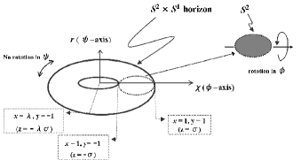
Figure 1: Schematic diagram of a local ringlike object which resides in the spacetime. Generally some singular behavior appears near the horizon.

The spacetimes generally have some local gravitational objects which one may regard as black holes. Analyzing the rod structure, which was studied for the higher-dimensional Weyl solutions by Emparan and Reall ref8 and for the nonstatic solutions by Harmark refHAR , we can show that there are event horizons at $x=1$ in these spacetimes. In fact, there is a finite timelike rod for $z\in[-\sigma,\sigma]$ with the direction

$$v=(1,\Omega,0),~{}~{}~{}\Omega=\frac{(1+\alpha\beta)((\lambda+1)\alpha-2\beta)}{2\sigma^{\frac{1}{2}}((\lambda+1)\alpha^{2}+2)},$$ (12)

which corresponds to the region of time translational invariance. The topology of the event horizon is $S^{2}\times S^{1}$ for $\lambda>1$ as in Figure 1, if it is free of the pathology of the Dirac-Misner string Elvang:2004xi . We will discuss this later.

As naturally expected from the presence of the rotation, the new rings have ergo-regions. In fact, the 0-0 component of the metric (8) becomes positive near $x=1$ because the function $A$ becomes negative there. The limiting form of this componet at $x=1$ is obtained as

$$g_{00} = \frac{((\lambda+1)\alpha-2\beta)^{2}(1-y^{2})}{(8(\lambda+y)+(2\beta(1-y)+\alpha(\lambda+1)(1+y))^{2}}.$$

We show the typical behavior of this componet in FIG.2.

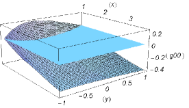
Figure 2: The behavior of $0$-$0$ component of the metric in the case of $(\alpha,\,\beta,\,\lambda)=(1/2,\,-0.195752,\,2)$. The region where the component function is above the level zero corresponds to the ergo-region.

Here we consider the appearance of CTC-regions where the $\phi$-$\phi$ component of the metric becomes negative. At first it can be easily shown that the value of $g_{\phi\phi}$ is zero at $y=1$. There is no harmful feature around there. However we can confirm the appearance of CTC from the fact that the functional form of this component becomes

$$g_{\phi\phi}=-\frac{4\sigma(2\alpha\beta^{2}+(2+\alpha^{2}(\lambda+1))\beta+\alpha(\lambda-1))^{2}(x^{2}-1)}{(1+\alpha\beta)^{2}(8\beta^{2}(\lambda-x)+((\lambda-1)(x+1)+\alpha\beta(\lambda+1)(x-1))^{2})},$$ (14)

for the ranges $1<x<\lambda$ at $y=-1$. This value is always negative except when the parameters satisfy the following condition

$$2\alpha\beta^{2}+(2+\alpha^{2}(\lambda+1))\beta+\alpha(\lambda-1)=0.$$ (15)

When $\lambda$ and $\alpha$ are given, the parameter $\beta$ should be

$$\beta = \beta_{+}$$

$$= -\frac{2+{\alpha}^{2}({\lambda}+1)+\sqrt{{\alpha}^{4}({\lambda}+1)^{2}-4{\alpha}^{2}({\lambda}-3)+4}}{4{\alpha}},$$

or

$$\beta = \beta_{-}$$

$$= -\frac{2+{\alpha}^{2}({\lambda}+1)-\sqrt{{\alpha}^{4}({\lambda}+1)^{2}-4{\alpha}^{2}({\lambda}-3)+4}}{4{\alpha}}.$$

When the parameters satisfy the condition (15) the solution is free of the pathology of the Dirac-Misner string Elvang:2004xi . Even in this case there can appear the CTC when the function $B$ becomes sufficiently small outside the ergo region. We can show that the value of $B$ becomes zero at

$$x=\frac{(\lambda^{2}-1)\alpha^{2}-4\beta^{2}}{4\alpha\beta},~{}~{}~{}y=0.$$ (18)

For $\beta=\beta_{+}$, the coordinate value $x$ of (18) is in its range $x>1$. Therefore there appears singular behavior and $g_{\phi\phi}$ becomes negative in its neighborhood. While, when $\beta=\beta_{-}$, this singular behavior does not appear because $x<1$. As a result, the condition (LABEL:eq:noCTC) makes the singular structure of the spacetimes fairly mild as seen in FIG. 3, where the CTC-region which generally appears near the horizon disappears.

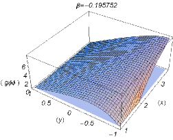
Figure 3: The behavior of $\phi$-$\phi$ component of the metric in the case of $(\alpha,\,\beta,\,\lambda)=(1/2,\,-0.195752,\,2)$ which satisfies the Eq.(LABEL:eq:noCTC). The corresponding component always has non-negative values, while for general case the component becomes negative near the horizon, which means the existence of CTC-regions.

Even for this case, there exists a kind of strut structure in this spacetime. The reason for this is that the effect of rotation cannot compensate for the gravitational attractive force. The periods of the coordinates $\psi$ and $\phi$ should be defined as

$$\Delta\psi=2\pi\lim_{\chi\rightarrow 0}\sqrt{\frac{\chi^{2}g_{\chi\chi}}{g_{\psi\psi}}}~{}~{}~{}\mbox{and}~{}~{}~{}\Delta\phi=2\pi\lim_{r\rightarrow 0}\sqrt{\frac{r^{2}g_{rr}}{g_{\phi\phi}}},$$

to avoid a conical singularity. Both $\Delta\psi$ and $\Delta\phi$ for $y=1$, i.e. outside the ring, are $2\pi$. While the period of $\phi$ inside the ring becomes

$$\Delta\phi=2\pi\frac{\lambda-1+(\lambda+1)\alpha\beta}{\sqrt{\lambda^{2}-1}(1+\alpha\beta)},$$

which is less than $2\pi$ for $1<\lambda<\infty$ with real $\alpha$. Hence, two-dimensional disklike struts, which appear in the case of static rings ref8 , are needed to prevent the collapse of the rings.

When ${\lambda}=1$ and $\beta=0$, the metric is reduced to the form found by Myers and Perry refMP which describes a one-rotational spherical black hole in five dimensions. In fact the metric has the following expression,

$$ds^{2} = -\frac{p^{2}x+q^{2}y-1}{p^{2}x+q^{2}y+1}\left(dx^{0}+2\sigma^{1/2}\,\frac{q}{p}\,\frac{1-y}{p^{2}x+q^{2}y-1}d\phi\right)^{2}$$ (19)

$$+\sigma\,\,\frac{p^{2}x+q^{2}y+1}{p^{2}x+q^{2}y-1}\,(x-1)\,(1-y)\,d\phi^{2}$$

$$+\sigma(x+1)\,(1+y)\,d\psi^{2}$$

$$+{\sigma}\frac{p^{2}x+q^{2}y+1}{2p^{2}}\left[\frac{dx^{2}}{x^{2}-1}+\frac{dy^{2}}{1-y^{2}}\right],$$

where $p^{2}=1/({\alpha}^{2}+1)$ and $q^{2}={\alpha}^{2}/({\alpha}^{2}+1)$. Introduce new parameters $a_{0}$ and $m$ through the relations,

$$p^{2}=\frac{4\sigma}{m^{2}},\ \ q^{2}=\frac{a_{0}^{2}}{m^{2}},$$

so the metric (19) is transformed into

$$ds^{2} = -(1-\Delta)\left[dx^{0}+\frac{a_{0}\Delta\sin^{2}\theta}{1-\Delta}d\phi\right]^{2}$$ (20)

$$\hskip-8.5359pt\,+\,\frac{1}{1-\Delta}\left[\tilde{r}^{2}+(m^{2}-a_{0}^{2})\right]\sin^{2}\theta\,d\phi^{2}+\tilde{r}^{2}\cos^{2}\theta\,d\psi^{2}$$

$$\hskip-8.5359pt\,+\,(\tilde{r}^{2}+a_{0}^{2}\cos^{2}\theta)\left[d\theta^{2}+\frac{d\tilde{r}^{2}}{\tilde{r}^{2}-(m^{2}-a_{0}^{2})}\right],$$

where $\Delta:=m^{2}/(\tilde{r}^{2}+a_{0}^{2}\cos^{2}\theta)$. The line-element (20) is exactly the same form found by Myers and Perry.

In some limiting cases with the relation (LABEL:eq:noCTC), the corresponding solutions are reduced to the well-known solutions like the static black rings or the rotational black strings corresponding to (four-dimensional Kerr spacetime) $\times$ R. The former case is realized when we take the limit ${\alpha}\rightarrow 0$ and the latter is realized when the parameter $\lambda$ goes to infinity under the condition: ${\alpha}=\tilde{{\alpha}}\times\sqrt{2/\lambda}$ with $-1<\tilde{{\alpha}}<1$.

Finally we comment on the four independent parameters. The parameters $\lambda$ and $\sigma$ characterize the size and mass of the local object which resides in the spacetime. Appropriate combinations of $\alpha$ and $\beta$ can be considered as the Kerr-parameter and the NUT-parameter in four-dimensional case. For example, the five-dimensional analogue of Kerr-NUT solution is obtained by setting $\lambda=1$. In this case the parameter $\beta$ can be considered as a NUT-like parameter because, as we have already shown, the one-rotational Myers-Perry solution is realized when $\beta=0$. Also in the case of string like solution, $\lambda\rightarrow\infty$, the four-dimensional part of this solution corresponds with the Kerr solution when $\alpha=-\beta$ and with the NUT solution when $\alpha=\beta$.

V summary

In this letter, we generated the new axisymmetric stationary solutions of five-dimensional vacuum Einstein equations from the five-dimensional Minkowski spacetime as the simplest seed spacetime. In particular we found a candidate of another branch of one-rotational “black rings”. Systematic analysis of the new solutions will be presented refIM .

In the method presented here we can also adopt other seed spacetimes, so that we can find some new spacetimes. However it should be noticed that the method introduced here can not be used for the solution-generation of black rings with rotation in two independent planes because of the metric form (1). For this purpose other methods may be used. One of the most powerful methods would be the inverse scattering method refBZ , which was applied to a five-dimensional string theory system Herrera-Aguilar:2003ui and static five-dimensional cases Koikawa:2005ia .

- (1) S. B. Giddings and S. Thomas, Phys. Rev. D 65, 056010 (2002).
- (2) M. I. Cai and G. J. Galloway, Class. Quant. Grav. 18, 2707 (2001); G. W. Gibbons, D. Ida, and T. Shiromizu, Phys. Rev. Lett. 89, 041101 (2002); Y. Morisawa and D. Ida, Phys. Rev. D 69, 124005 (2004).
- (3) H. Elvang, N. Obers and T. Harmark, Class. Quant. Grav. 21, S1509 (2004).
- (4) H. Elvang, T. Harmark and N. A. Obers, JHEP 0501, 003 (2005).
- (5) B. Kol, Phys. Rept. 422, 119 (2006)
- (6) R. Emparan and H. S. Reall, Phys. Rev. Lett. 88, 101101 (2002).
- (7) H. Elvang, R. Emparan, D. Mateos and H. S. Reall, Phys. Rev. Lett. 93, 211302 (2004); J. P. Gauntlett and J. B. Gutowski, Phys. Rev. D 71, 025013 (2005); Phys. Rev. D 71, 045002 (2005).
- (8) D. Ida and Y. Uchida, Phys. Rev. D 68, 104014 (2003); H. K. Kunduri and J. Lucietti, Phys. Lett. B 609, 143 (2005); M. Ortaggio, JHEP 0505, 048 (2005).
- (9) R. Emparan, JHEP 0403, 064 (2004)
- (10) H. Stephani, D. Kramer, M. MacCallum, C. Hoenselaers and E. Herlt, Exact Solutions of Einstein’s Field Equations, 2nd ed. (Cambridge University Press, Cambridge, 2003).
- (11) D. Kramer and G. Neugebauer, Phys. Lett. A 75, 259 (1980).
- (12) A. Tomimatsu and H. Sato, Phys. Rev. Lett. 29, 1344 (1972).
- (13) V. Belinski and R. Ruffini, Phys. Lett. B 89, 195 (1980); W. Bruckman, Phys. Rev. D 36, 3674 (1987); T. Koikawa and K. Shiraishi, Prog. Theor. Phys. 80, 108 (1988).
- (14) P. O. Mazur and L. Bombelli, J. Math. Phys. 28, 406 (1987).
- (15) T. Dereli, A. Eriş and A. Karasu, Nuovo Cimento B 93, 102 (1986).
- (16) W. Bruckman, Phys. Rev. D 34, 2990 (1986).
- (17) T. Harmark, Phys. Rev. D 70, 124002 (2004).
- (18) F. J. Ernst, Phys. Rev. 167, 1175 (1968).
- (19) G. Neugebauer, J. Phys. A 13, L19 (1980).
- (20) C. Hoenselaers, W. Kinnersley and B. C. Xanthopoulos, J. Math. Phys. 20, 2530 (1979).
- (21) J. Castejon-Amenedo and V. S. Manko, Phys. Rev. D 41, 2018 (1990).
- (22) R. Emparan and H. S. Reall, Phys. Rev. D 65, 084025 (2002).
- (23) H. Elvang, R. Emparan and P. Figueras, JHEP 0502, 031 (2005).
- (24) R. C. Myers and M. J. Perry, Annals Phys. 172, 304 (1986).
- (25) H. Iguchi and T. Mishima, in preparation.
- (26) V. A. Belinskii and V. E. Zakharov, Zh. Exsp. Theor. Fiz. 77, 3 (1979).
- (27) A. Herrera-Aguilar and R. R. Mora-Luna, Phys. Rev. D 69, 105002 (2004).
- (28) T. Koikawa, Prog. Theor. Phys. 114, 793 (2005).