Abstract

We present a triangulation–independent area–ordering prescription which naturally generalizes the well known path ordering one. For such a prescription it is natural that the two–form “connection” should carry three “color” indices rather than two as it is in the case of the ordinary one–form gauge connection. To define the prescription in question we have to define how to exponentiate a matrix with three indices. The definition uses the fusion rule structure constants.

1 Introduction

Among the questions standing in front of the modern mathematical physics there are two which are of interest for us in this note:

• What is the theory of non–Abelian tensor fields?

• How to define “multiple–time” Hamiltonian formalism for non–point–like objects?

We argue in this note that these two questions are related to each other.

To define the theory of the two–tensor field we would like to understand its nature. We think that the appropriate point of view on the tensor field is to consider it as a connection on an unusual “fiber bundle”. Or, better to say, we present a somewhat different way of looking at known type of fiber bundles, where the two–tensor field acquires its natural place. The base of this bundle is the loop space ${\cal L}X$ of a finite–dimensional space $X$. A “point” of the space ${\cal L}X$ is the loop $\gamma$ on the space $X$. A “path” connecting two “points” $\gamma_{1}$ and $\gamma_{2}$ of the base ${\cal L}X$ is the surface $\Sigma(\gamma_{1},\,\gamma_{2})$ inside the space $X$. The surface $\Sigma(\gamma_{1},\,\gamma_{2})$ has cylindrical topology with the two end–loops $\gamma_{1}$ and $\gamma_{2}$.

Hence, the connection on this bundle $\hat{B}$ is a two–form which has to be integrated over the surface $\Sigma$. This is similar to the standard situation with the string two–tensor $B$–field. However, unlike that situation we would like to consider such fibers $V$ (sitting at each of the points of the loops $\gamma_{1}$ and $\gamma_{2}$), which have dimensionality bigger than one. Hence, the $\hat{B}$ field in this case carries “color” indices. As well the corresponding “holonomy matrix” of the $\hat{B}$ connection over the “path” $\Sigma$ has continuous number of indices distributed on the end–loops $\gamma$’s. To define the holonomy of the $\hat{B}$ field we have to define the area–ordering prescription.

We are not trying to formalize those concepts rather we would like to present an explicit construction of the objects listed in the previous paragraph. To define the area–ordering we consider a triangulation $\tilde{\Sigma}$ of the Riemann surface $\Sigma$. In this case the area–ordering is obtained via gluing over the whole simplicial surface exponents of $\hat{B}$’s assigned to each simplex. But from this picture it is obvious that the exponents should carry three indices in accordance with three wedges of each simplex — triangle. The question is what is the exponent which has three indices? To move further we suppose that this is a new object — a function of the matrix $\hat{B}$ which has three indices as well. We are going to define this function in this note. To define it we have to obey the main properties necessary to make the construction in question meaningful. The construction is meaningful if the prescription of the area–ordering does not depend on the way the continuum limit (from $\tilde{\Sigma}$ to $\Sigma$) is taken: We refer to this fact as the triangulation independence of the definition of the area–ordering.

Thus, the main difficulty for this definition is the absence of the understanding of how to exponentiate matrices with three indices. In this note we give a definition of such an exponent. To give an idea of this exponent and of the “triangulation independence”, let us recall that the exponent of a matrix ${A_{i}}^{j}$ with two indices has the following main feature:

$${\left(e^{t_{1}\,\hat{A}}\right)_{i}}^{j}\,{\left(e^{t_{2}\,\hat{A}}\right)_{j}}^{k}={\left(e^{\left(t_{1}+t_{2}\right)\,\hat{A}}\right)_{i}}^{k}$$ (1)

for any two numbers $t_{1}$ and $t_{2}$. This equation defines the exponent unambiguously. In fact, from this equation one can derive the differential equation for the exponent.

The exponent of a matrix $B_{ijk}$ with three indices can have any number of external indices (not only zero or two as the exponent of a matrix with two indices). As the result it obeys many different identities following from the conditions of the triangulation independence. Furthermore, the function of the three–linear form $B$ in question is not really an exponent in commonly accepted sense, but we refer to it as “exponent” for the reason it obeys such conditions of triangulation independence.

The most beautiful identity obeyed by the exponent in question is as follows:

$${\left(E^{t_{1}\,\hat{B}}\right)_{j_{1}\,k_{2}}}^{k_{1}}\,{\left(E^{t_{2}\,\hat{B}}\right)_{j_{2}\,k_{3}}}^{k_{2}}\,{\left(E^{t_{3}\,\hat{B}}\right)_{j_{3}\,k_{1}}}^{k_{3}}=\left(E^{\left(t_{1}+t_{2}+t_{3}\right)\,\hat{B}}\right)_{j_{1}\,j_{2}\,j_{3}},$$ (2)

which is shown graphically in the fig. 1. This equation, however, does not define unambiguously the exponent of the matrix $\hat{B}$ with three indices.

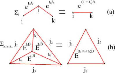
Figure 1: Main properties of the exponents.

However, it is this point where the formalism which we develop can help in establishing “two–time” Hamiltonian formalism. We briefly discuss this point in concluding section. A more complete discussion will be given in another publication.

It is worth mentioning at this point that the area–ordering can be defined via the standard exponent for a two–tensor form with two “color” indices. But such a definition demands as well the presence of an additional one–form gauge connection [1]. Hence, if we would like to deal with the two–tensor field only we have to follow our line of reasoning.

The organization of the paper is as follows. In the section 2 we present our prescription of the area–ordering. In the section 3 we define how to exponentiate matrices with three indices. In the section 4 we discuss the properties of the area–ordering and of the “fiber bundle” in question. In this section as well we present other definitions of the exponent. In the section 5 we present some explicit examples of the $I$ and $\kappa$ matrices to be defined in the main body of the text. We end up with conclusions and brief discussion of some future direction (such as development of the “two–time” Hamiltonian formalism). Appendix contains some necessary explicit calculations.

2 Area–ordering and triangulations

To set the notations and to present the idea of our argument let us describe briefly how one obtains the path ordering. Consider the base space $X$ of a vector bundle with $N$–dimensional fibers $V$. We would like to find the holonomy matrix, corresponding to a path $\gamma_{xy}$, which relates $N$–vectors in fibers over two points (say $x$ and $y$) of the $X$ space. We give here a somewhat weird way of defining the path ordered exponent, which, however, is easy to generalize to the two–dimensional case. To define the holonomy matrix we approximate the path $\gamma_{xy}$ by a broken line $\tilde{\gamma}_{xy}$, consisting of a collection of small straight lines (see fig. 2).

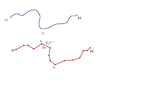
Figure 2: $\tilde{\gamma}_{xy}$ is the discretization of $\gamma_{xy}$. On each wedge of $\tilde{\gamma}$ there is ${U_{k_{l}}}^{k_{(l+1)}}$.

The holonomy in question is given by:

$${U\left(\tilde{\gamma}_{xy}\right)_{i}}^{j}\equiv\sum^{N}_{k_{1},k_{2},\dots,k_{L}}{U\left(x,\Delta_{1}x\right)_{i}}^{k_{1}}\,{U\left(x_{1},\Delta_{2}x\right)_{k_{1}}}^{k_{2}}\dots U(y,\Delta_{L}x)_{k_{L}}^{j},$$ (3)

where $L$ is the number of wedges of the broken line; $x_{1}=x+\Delta_{1}x$, etc. and $\Delta_{l}x$ is the $l$-th wedge of the broken line; each $U$ in eq.(3)  is an operator $\hat{U}:V\to V$. From now on small Latin letters ($i,j,k$ etc.) represent “color” indices running from $1$ to $N$.

To obtain the holonomy for the path $\gamma_{xy}$ itself we have to take the continuum limit $L\to\infty$ and $\left|\Delta_{l}x\right|\to 0$, $l=1,...,L$. This definition does not depend on the one–dimensional triangulation, i.e. on the concrete choice of the sequence of $\tilde{\gamma}_{xy}$’s in approaching $\gamma_{xy}$ as $L\to\infty$. This is true due to the fact that each $U$ in the product (3) can be represented as the exponent of an element of the algebra — the connection of the vector bundle. The definition of the exponent is (do not confuse it with the path ordered exponent):

$${U_{i}}^{j}={\left(e^{\hat{A}}\right)_{i}}^{j}\equiv\lim_{M\to\infty}{\left(\prod_{\rm graph}^{M}\left[1+\frac{\hat{A}}{M}\right]\right)_{i}}^{j}\equiv$$

$$\equiv\lim_{M\to\infty}\left({\delta_{i}}^{j_{1}}+\frac{{A_{i}}^{j_{1}}}{M}\right)\left({\delta_{j_{1}}}^{j_{2}}+\frac{{A_{j_{1}}}^{j_{2}}}{M}\right)\dots\left({\delta_{j_{M}}}^{j}+\frac{{A_{j_{M}}}^{j}}{M}\right)=$$

$$\lim_{M\to\infty}\left[{\left(\prod_{\rm graph}^{M}\delta\right)_{i}}^{j}+\frac{1}{M}\,\sum_{a=1}^{M}{A_{k}}^{m}(a)\left(\prod_{{\rm graph}(a)}^{M-1}\delta\right)_{m\,i}^{k\,j}+\frac{1}{M^{2}}\,\sum_{a\neq b=1}^{M}{A_{k}}^{m}(a)\,{A_{n}}^{l}(b)\left(\prod_{{\rm graph}(a,b)}^{M-2}\delta\right)_{l\,m\,i}^{n\,k\,j}\right.$$

$$\left.+{\cal O}\left(\frac{1}{M^{3}}\right)\right]={\delta_{i}}^{j}+{A_{i}}^{j}+\frac{1}{2!}\,{\left(\hat{A}^{2}\right)_{i}}^{j}+{\cal O}\left(\frac{1}{3!}\right)$$ (4)

where the case of interest for us is when ${A_{i}}^{j}={A_{\mu\,i}}^{j}(x)\,\Delta x^{\mu}$ but in this formula we consider $A$ as a constant matrix. In this expression the limit is taken over a sequence of open, connected graphs (broken lines) with $M$ wedges; to each wedge we assign $(1+\hat{A}/M)$ and glue them via contraction of lower and upper indices; in the second term of the third line we sum over all possible insertions (enumerated by $a$) of one $\hat{A}$ into the graph; $A(a)$ means just the matrix $A$ placed in the $a$–th wedge; graph$(a)$ is a disconnected broken line — the original graph without the $a$–th wedge; in the third term of the third line we sum over all possible insertions of the couple of $\hat{A}$’s into the graph; graph$(a,b)$ is a disconnected broken line — the original graph without the $a$–th and $b$–th wedges. The products of $\delta$’s in eq.(4)  are taken over these graphs in the obvious way: Via contraction of lower and upper indices.

It is this definition of the exponent which makes the path ordering (3) triangulation independent in the limit $L\to\infty$. In fact, the matrix ${\delta_{i}}^{j}$ solves the equation

$${\kappa_{i}}^{j}\,{\kappa_{j}}^{k}={\kappa_{i}}^{k},$$ (5)

graphically represented in fig. 3. As the result all products of $\delta$’s in eq.(4)  are equal to $\delta$ itself: $\prod\delta=\delta$.

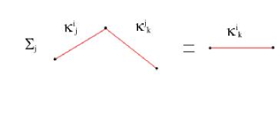
Figure 3: The one–dimensional condition for the triangulation independence.

Any solution of the eq.(5)  is suitable to define the exponent of a matrix with two indices and, hence, the triangulation independent path ordering. The generic solution to this equation is just a projection operator. Hence, the definition of the exponent with such a projector is just a standard one when restricted to the eigen–space of the projector. Using eq.(5)  we obviously obtain that in the limit in question:

$${U\left(\gamma_{xy}\right)_{i}}^{j}={\left(Pe^{\int_{0}^{2\pi}ds\,\hat{A}_{\mu}(x)\,\dot{x}^{\mu}(s)}\right)_{i}}^{j}\equiv$$

$$\equiv{\delta_{i}}^{j}+\int_{0}^{2\pi}ds\,{A_{\mu\,i}}^{j}(x)\,\dot{x}^{\mu}(s)+\int_{0}^{2\pi}ds_{1}\int_{0}^{s_{1}}ds_{2}\,{A_{\mu\,i}}^{k}(x)\,\dot{x}^{\mu}(s_{1})\,{A_{\nu\,k}}^{j}(x)\,\dot{x}^{\nu}(s_{2})+\dots,$$ (6)

where $x(s)$ is the map (of $s\in[0,2\pi)$ into $X$) whose image is the curve $\gamma_{xy}$; $x(0)=x,\,\,x(2\pi)=y$.

We would like to generalize this construction to the case of the ordering over two–dimensional surfaces. It is natural to consider, within this context, a triangulated approximation $\tilde{\Sigma}(\tilde{\gamma_{1}},\dots,\tilde{\gamma_{L}})$ of an oriented Riemann surface $\Sigma(\gamma_{1},\dots,\gamma_{L})$ with $L$ boundary closed loops $\gamma$’s which are approximated by the closed broken lines $\tilde{\gamma}$’s (see fig. 4).

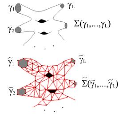
Figure 4: $\tilde{\Sigma}$ is the discretization of $\Sigma$; $\tilde{\gamma}$’s are discretizations of $\gamma$’s.

Similarly to the one–dimensional case, in which we assign ${U_{i}}^{j}$ to each simplex (wedge), in this two–dimensional case we assign $U_{ijk}$ to each simplex (triangle). At the same time the indices $i,j$ and $k$ are assigned to the three wedges of the corresponding triangle. Hence, in this case $\hat{U}:V^{3}\to\mathbb{C}$ for an $N$–dimensional vector space $V$ — the “fiber” of our ”fiber bundle”.

If we consider cyclicly symmetric $U_{ijk}$ then the area–ordering prescription is unambiguous. The area–ordering is obtained by gluing, via the use of a bi–linear form $\kappa^{ij}:\mathbb{C}\to V^{2}$, the matrices $U_{ijk}$ on each simplex over the whole simplicial surface (see fig. 5):

$$U\left[\tilde{\Sigma}(\tilde{\gamma_{1}},\dots,\tilde{\gamma_{L}})\right]_{j^{(1)}_{1}\dots j^{(1)}_{n_{1}}\left|j^{(2)}_{1}\dots j^{(2)}_{n_{2}}\right|\dots\left|j^{(L)}_{1}\dots j^{(L)}_{n_{L}}\right.}\equiv$$

$$\equiv\sum_{k_{1},k_{2},\dots,k_{w}}U_{j^{(1)}_{1}\,k_{1}\,k_{2}}\left(x_{1}^{\phantom{\frac{1}{2}}},\Delta\sigma_{1}\right)\,{U^{k_{1}\,k_{3}}}_{k_{4}}\left(x_{2}^{\phantom{\frac{1}{2}}},\Delta\sigma_{2}\right)\,{U^{k_{3}}}_{j^{(1)}_{2}\,j^{(1)}_{3}}\left(x_{3}^{\phantom{\frac{1}{2}}},\Delta\sigma_{3}\right)\dots$$ (7)

where $w$ is the total number of internal wedges of the graph; $j^{(l)}$ are the indices corresponding to the wedges of the $l$-th broken line $\tilde{\gamma}_{l}$ and $n_{l}$ is the total number of its wedges, correspondingly. We higher (lower) the indices via the use of the aforementioned bilinear form $\kappa^{ij}$ ($\kappa_{ij}\kappa^{jk}=\delta_{i}^{k}$); $\Delta\sigma$’s are elementary oriented areas associated to the triangles.

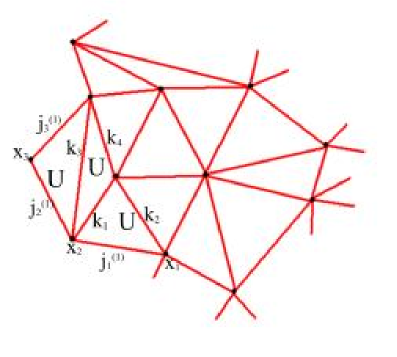
Figure 5: This is a part of $\tilde{\Sigma}(\tilde{\gamma}_{1},\dots,\tilde{\gamma}_{L})$. On each triangle of this figure there is $U$ matrix with three indices and we sum over indices assigned to the internal wedges of the graph.

In the continuum limit the discrete indices $1,...,n_{l}$ are converted into the continuum ones $s_{l}\in[0,\,2\pi)$ and we obtain:

$$U\left[\tilde{\Sigma}(\tilde{\gamma_{1}},\dots,\tilde{\gamma_{L}})\right]_{j^{(1)}_{1}\dots j^{(1)}_{n_{1}}\left|j^{(2)}_{1}\dots j^{(2)}_{n_{2}}\right|\dots\left|j^{(L)}_{1}\dots j^{(L)}_{n_{L}}\right.}\longrightarrow U\left[\Sigma^{\phantom{\frac{1}{2}}}(\gamma_{1},\dots,\gamma_{L})\right]_{j^{(1)}(s_{1})\left|j^{(2)}(s_{2})\right|\dots\left|j^{(L)}(s_{L})\right.},$$

$${\rm where}\quad\hat{U}(\Sigma):V^{\infty}(1)\otimes\dots\otimes V^{\infty}(L)\to\mathbb{C},$$ (8)

and $j^{(l)}(s_{l})$ is the “color” index assigned to the continuous number of points enumerated by $s_{l}$ — a parametrization of the $l$-th loop $\gamma_{l}$. Such an operator $\hat{U}(\Sigma)$ for $L=1$ is graphically represented in fig. 6.

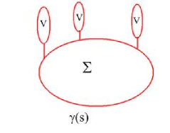
Figure 6: At each point $s$ of the curve $\gamma$ there is the fiber $V$.

The expression (8) is not so unfamiliar for the string theoreticians as it could seem from the first sight. In fact, if we substitute $j^{(l)}(s_{l})$ by $x^{(l)}(s_{l})$, then $U\left[\Sigma(\gamma_{1},\dots,\gamma_{L})\right]$ can be considered as the string amplitude whose end–loops $\gamma$’s are mapped by $x(s)$’s. This analogy is helpfull in understanding how our considerations could help in defining the “two–time” Hamiltonian formalism — the formalism for string–like objects. See short discussion on this subject in the concluding section.

Thus, we have defined the area–ordering prescription. But this is not the whole story: We have to define $U_{ijk}$ in such a way that the limit (8) exists and does not dependent on the triangulation, i.e. does not depend on the way it is taken.

3 Exponentiation of a matrix with three indices

In this section we show that for the continuum expression in eq.(8)  to be triangulation independent each $U_{ijk}$ should be represented as the exponent:

$$U_{ijk}=\left(E^{\hat{B}}\right)_{ijk},$$ (9)

where $\hat{B}$ is a matrix with three indices: particular case of interest for us is when $B^{ijk}(x,\Delta\sigma)=B^{ijk}_{\mu\nu}(x)\,\Delta x^{\mu}\,\Delta x^{\nu}$. It is natural to assume that $B$ as well as $U$ has three indices rather than any other number.

We take the generalization of (4) to define the exponent of a matrix with three indices:

$${\rm Tr}\,\left(E^{\hat{B}}_{g,I,\kappa}\right)\equiv\lim_{M\to\infty}\prod_{{\rm graph},g}^{M}\left(\hat{I}+\frac{\hat{B}}{M}\right),$$ (10)

where the limit is taken over any sequence of closed (because on the LHS we take Tr), connected, oriented triangulation graphs of genus $g$ and with $M$ faces (triangles). To take the limit $M\to\infty$ we have to choose a sequence of graphs. There is no any distinguished sequence of graphs. Hence, we have to demand somehow that the result of the limit (10) should not depend on the chosen sequence of graphs.

We are going to explain now the conditions (including the ones imposed on the matrices $\kappa^{ij}$ and $I_{ijk}$), under which the limit (10) does not depend on the chosen sequence of graphs. First, we demand that in these graphs any two triangles can not meet (glued) at more than one wedge (see fig. 7). Second, as the limit $M\to\infty$ is taken the number of triangles meeting at any vertex of the graph should be suppressed in comparison with $M$. This condition is necessary to overcome the difficulty discussed in the Appendix.

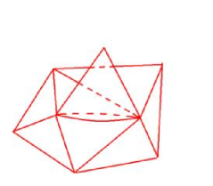
Figure 7: No such configurations inside the graphs defining the exponent.

As we show below the definition of the exponent (10) does depend on the choice of matrices $\hat{I}$, $\kappa$ and the genus $g$ of the graphs in the sequence, along which the limit $M\to\infty$ is taken. Due to this fact we designate the definition of the exponent in eq.(10)  with the corresponding subscripts. At fixed $M$ the product in eq.(10)  is taken over the graph in question: Meaning that at each face of the graph we put matrix $(I+B/M)_{ijk}$ and we glue indices of these matrices with the use of the aforementioned bilinear form $\kappa^{ij}$. The matrices $I_{ijk}$ and $\kappa^{ij}$ we are going to define in a moment.

We start our consideration with an arbitrary oriented graph with the spherical topology ($g=0$) and $M$ faces: All our considerations below can be easily generalized to the case of arbitrary graphs with higher topology. Let us expand the product in eq.(10)  for such a particular choice of the graph:

$$\prod_{\rm graph,0}^{M}\left(\hat{I}+\frac{\hat{B}}{M}\right)=\prod_{\rm graph}^{M}\hat{I}+\frac{1}{M}\sum_{a=1}^{M}B^{j_{1}\,j_{2}\,j_{3}}(a)\,\left(\prod_{{\rm graph}(a)}^{M-1}\hat{I}\right)_{j_{3}\,j_{2}\,j_{1}}+$$

$$+\frac{1}{M^{2}}\left[\sum^{(I)}_{a\neq b}B^{j_{1}\,j_{2}\,j_{3}}(a)\,B^{j_{4}\,j_{5}\,j_{6}}(b)\,\left(\prod_{{\rm graph}(I,a,b)}^{M-2}\hat{I}\right)_{j_{3}\,j_{2}\,j_{1}\left|j_{6}\,j_{5}\,j_{4}\right.}\right.+$$

$$+\sum^{(II)}_{a\neq b}B^{j_{1}\,j_{2}\,j_{3}}(a)\,B^{j_{4}\,j_{5}\,j_{6}}(b)\,\left(\prod_{{\rm graph}(II,a,b)}^{M-2}\hat{I}\right)_{j_{6}\,j_{5}\,j_{4}\,j_{3}\,j_{2}\,j_{1}}+$$

$$\left.+\sum^{(III)}_{a\neq b}B^{j_{1}\,j_{2}\,k}(a)\,{B_{k}}^{\,j_{3}\,j_{4}}(b)\,\left(\prod_{{\rm graph}(III,a,b)}^{M-2}\hat{I}\right)_{j_{4}\,j_{3}\,j_{2}\,j_{1}}\right]+{\cal O}\left(\frac{1}{M^{3}}\right),$$ (11)

where the first term represents the product of $\hat{I}$’s over the graph and it is a constant independent of $\hat{B}$. The second term is the sum over the faces of the graph enumerated by $a$; $\hat{B}(a)$ means the matrix $\hat{B}$ placed in the face $a$ and the product of $\hat{I}$’s in this term is taken over the graph$(a)$, which is the original graph without the face $a$ (see fig. 8). In the third term the sum ($\sum^{(I)}$) is taken over the remote faces $a$ and $b$ (see fig. 9). Hence, the graph$(I,a,b)$ (the original graph without $a$ and $b$ faces) has the cylindrical topology with three external wedges at each end of the cylinder: This is the reason why we divide the subscript in the corresponding term into two groups $j_{1}\,j_{2}\,j_{3}$ and $j_{4}\,j_{5}\,j_{6}$ (we come back to this point later). At the same time, in the fourth and fifth terms the sums ($\sum^{(II)},\sum^{(III)}$) are taken over the adjacent faces $a$ and $b$. Hence, the graphs$(II,III,a,b)$ have disc topology (see fig. 10 (a) and (b)). In the third term the faces $a$ and $b$ are touching each other via one common vertex (see fig. 10 (a)). In the fourth term the faces $a$ and $b$ are touching each other via one common wedge (see fig. 10 (b)). The terms $\propto B_{i\,k_{1}\,k_{2}}\,{B^{k_{1}\,k_{2}}}_{j}$ do not appear in eq.(11)  for the reason that we do not consider the graphs having the configuration of triangles shown in the fig. 7.

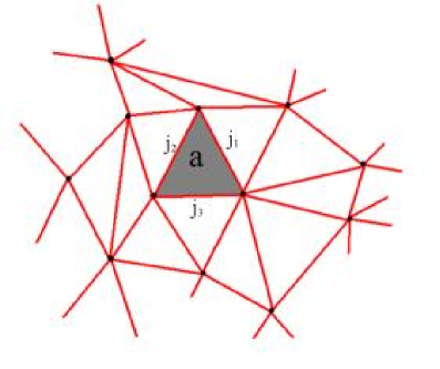
Figure 8: This is a part of the graph with the disc topology — the original spherical graph without the face $a$.

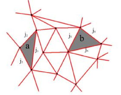
Figure 9: This is a part of the graph with the cylindrical topology — the original spherical graph without $a$ and $b$ faces.

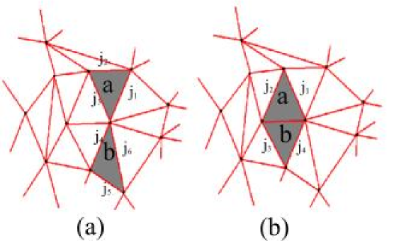
Figure 10: There are two possibilities how two triangles can meet each other inside the triangulation graph.

We would like to choose such matrices $I_{ijk}$ and $\kappa^{ij}$ that the expression (11) has a well defined limit as $M\to\infty$. It appears that to reach this goal is the same as to make the continuum expression (8) independent of triangulation [3]. It is this moment when we have to recall eq.(5) . We have to write an analog of this equation for $\hat{I}$ and $\hat{\kappa}$: So that various triangulations of the graphs with the same topology will be equal to each other. The analog of eq.(5)  for this case is $I_{ijk}$:

$$\sum_{j,k=1}^{N}{I_{ij}}^{k}\,{I_{lk}}^{j}=\kappa_{il}$$

$$\sum_{n=1}^{N}I_{inl}\,{I^{n}}_{jk}=\sum_{n=1}^{N}I_{ijn}\,{I^{n}}_{kl}.$$ (12)

The graphical representation of these equations (in terms of dual three–valent graphs) one can find in the fig. 12. We will discuss various solution of the conditions (12) in the next section. Unlike the one dimensional case, where there is basically the unique solution to the eq.(5) , in this case we will have the whole zoo of solutions. Now let us see how these observations influence the definition of the exponent.

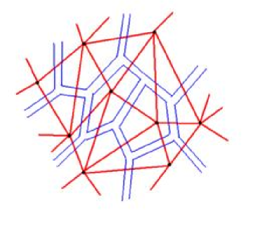
Figure 11: Duality relation between graphs. Dual graph is shown here by fat stripes.

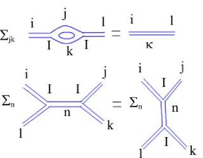
Figure 12: Two–dimensional conditions for the triangulation independence.

If these conditions are obeyed, one can map product of $\hat{I}$’s over any graph to the product of $\hat{I}$’s over any other graph with the same topology [3] (with the same genera, number of holes and distribution of external wedges among the holes). This can be straightforwardly seen by explicit manipulations with the dual graphs. For example, any graph with the disc topology and $n$ external wedges can be mapped to the graph shown in the fig. 13. At the same time, any graph with the annulus topology and $m$ wedges at one end and $k$ wedges at another end can be mapped to the graph shown in the fig. 14. The expressions for such two kinds of multiplications of $\hat{I}$’s are not equivalent to each other even if $n=k+m$. It is such facts which make us to distinguish the third and the fourth terms in eq.(11)  and to fix the genus $g$ of the graphs in the sequence to define the exponent.

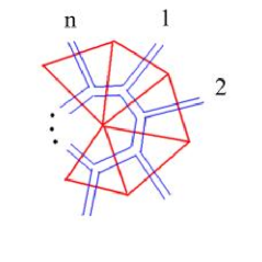
Figure 13: Disc topology.

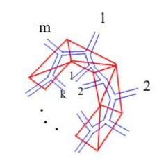
Figure 14: Annulus topology. Dual graph is shown for convenience of the understanding of the symmetries of the corresponding matrix: We can exchange the positions of say the line number $m$ and $k$ via the second relation shown in fig. 12. This fact should be compared with the property of the graph in fig. 13. There in general situation we have no means to exchange the positions of say the $n$–th and the $1$–st external legs.

Thus, if $I_{ijk}$ and $\kappa^{ij}$ obey eq.(12) , we obtain:

$$\prod_{\rm graph,0}^{M}\left(\hat{I}+\frac{\hat{B}}{M}\right)=N+B^{j_{1}\,j_{2}\,j_{3}}\,I_{j_{3}\,j_{2}\,j_{1}}+$$

$$+\frac{1}{M^{2}}\left[C_{1}(M)\,B^{j_{1}\,j_{2}\,j_{3}\phantom{\frac{1}{2}}}B^{j_{4}\,j_{5}\,j_{6}}\,I_{j_{3}\,j_{2}\,j_{1}\left|j_{6}\,j_{5}\,j_{4}\right.}\right.+C_{2}(M)\,B^{j_{1}\,j_{2}\,j_{3}}\,B^{j_{4}\,j_{5}\,j_{6}}\,I_{j_{6}\dots j_{1}}+$$

$$\left.+C_{3}(M)\,B^{j_{1}\,j_{2}\,k\phantom{\frac{1}{2}}}{B_{k}}^{\,j_{3}\,j_{4}}\,I_{j_{4}\dots j_{1}}\right]+{\cal O}\left(\frac{1}{M^{3}}\right),$$ (13)

where we denote by the same letter $I$ the product of the three–linear form $I_{ijk}$ over the corresponding graphs. $I_{j_{3}\,j_{2}\,j_{1}|j_{6}\,j_{5}\,j_{4}}$ is given by the annulus graph in fig. 15 where in each face stands matrix $I_{ijk}$. As can be seen explicitly from the dual graph representation, the matrix $I_{j_{3}\,j_{2}\,j_{1}|j_{6}\,j_{5}\,j_{4}}$ is cyclicly symmetric in the $j_{1},\,j_{2},\,j_{3}$ and $j_{4},\,j_{5},\,j_{6}$ indices separately. But otherwise one can exchange position of indices from these two groups in any order (see the discussion under the fig. 14). This property should be contrasted with the one of the matrix $I_{j_{6}\dots j_{1}}$ which is given by the disc graph in fig. 16. The matrix $I_{j_{6}\dots j_{1}}$ is symmetric under the cyclic exchange of all its six indices $j_{1},\dots,j_{6}$, but for generic choice of $I_{ijk}$ there is no any other symmetry. The same is true for the matrix $I_{j_{4}\dots j_{1}}$ which is given by the graph with disc topology, but with four external wedges: It is symmetric under the cyclic exchange of all its four indices.

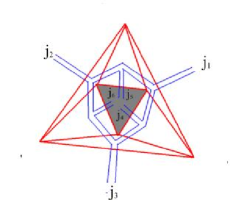
Figure 15: Graph for $I_{j_{3}\,j_{2}\,j_{1}|j_{6}\,j_{5}\,j_{6}}$. Dual graph is shown to explain the symmetry properties of the corresponding matrices.

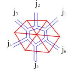
Figure 16: Graph for $I_{j_{6}\,j_{5}\,j_{4}\,j_{3}\,j_{2}\,j_{1}}$.

The constants $C_{1}(M)$, $C_{2}(M)$ and $C_{3}(M)$ are the numbers of the terms in the corresponding sums in eq.(11) . We calculate them in the Appendix and show that under conditions listed below the eq.(10)  the constants $C_{2}(M)$ and $C_{3}(M)$ are $\propto M$ and do not survive the limit $M\to\infty$ and

$$\frac{C_{1}(M)}{M^{2}}\to\frac{1}{2!}.$$

Similar story happens for the higher terms in $\hat{B}$ and higher genera (see the Appendix). As the result we obtain the following expression for the exponent:

$${\rm Tr}\,\left(E^{\hat{B}}_{g,I,\kappa}\right)=\sum_{F=0}^{\infty}\frac{1}{F!}\,B^{j^{(1)}_{1}\,j^{(1)}_{2}\,j^{(1)}_{3}}\dots B^{j^{(F)}_{1}\,j^{(F)}_{2}\,j^{(F)}_{3}}\,I^{g}_{j^{(1)}_{3}\,j^{(1)}_{2}\,j^{(1)}_{1}\left|\dots\right|j^{(F)}_{3}\,j^{(F)}_{2}\,j^{(F)}_{1}},$$ (14)

where $I^{g}_{j^{(1)}_{3}\,j^{(1)}_{2}\,j^{(1)}_{1}\left|\dots\right|j^{(F)}_{3}\,j^{(F)}_{2}\,j^{(F)}_{1}}$ is the matrix with $3F$ indices obtained via multiplication of $I_{ijk}$ over any oriented graph with $g$ handles, $F$ holes and 3 external wedges at each hole (see fig. 17). At the same time $I^{g},(F=0)$ is just a number obtained by the multiplication of $\hat{I}$ over the closed genus $g$ graph. For example, $I^{0}=\sum_{i}\delta_{i}^{i}=N$ because of the first relation in eq.(12) .

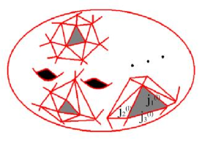
Figure 17: Triangulation graph defining $I^{g}$.

Similarly one can obtain the definition of the exponent for an open graph with any number of external wedges:

$$\left(E^{\hat{B}}_{g,I,\kappa}\right)_{\left.m^{(1)}_{1}\dots\,m^{(1)}_{n_{1}}\right|\dots\left|m^{(L)}_{1}\dots\,m^{(L)}_{n_{L}}\right.}=$$

$$=\sum_{F=0}^{\infty}\frac{1}{F!}\,B^{j^{(1)}_{1}\,j^{(1)}_{2}\,j^{(1)}_{3}}\dots B^{j^{(F)}_{1}\,j^{(F)}_{2}\,j^{(F)}_{3}}\,I^{g}_{\left.m^{(1)}_{1}\dots\,m^{(1)}_{n_{1}}\right|\dots\left|m^{(L)}_{1}\dots\,m^{(L)}_{n_{L}}\right|j^{(1)}_{3}\,j^{(1)}_{2}\,j^{(1)}_{1}\left|\dots\right|j^{(F)}_{3}\,j^{(F)}_{2}\,j^{(F)}_{1}},$$ (15)

where $I^{g}_{\left.m^{(1)}_{1}\dots\,m^{(1)}_{n_{1}}\right|\dots\left|m^{(L)}_{1}\dots\,m^{(L)}_{n_{L}}\right|j^{(1)}_{3}\,j^{(1)}_{2}\,j^{(1)}_{1}\left|\dots\right|j^{(F)}_{3}\,j^{(F)}_{2}\,j^{(F)}_{1}}$ is the matrix with $3F+n_{1}+\dots+n_{L}$ indices obtained via multiplication of $\hat{I}$’s over any oriented graph with $g$ handles, $L+F$ holes, 3 external wedges at $F$ holes and $n_{l}$ external wedges at $l$–th hole ($l=1,\dots,L$).

4 Properties of the area–ordering and other definitions of the exponent

Let us see now what kind of the area–ordering we obtain with such a definition of the exponent. The area–ordered exponent (“$A\,E$”) of the non–Abelian $B$–field over the disc $D$ is equal to:

$$U_{j(s)}(D,\hat{B})=\left(A\,E_{g,I,\kappa}^{{\int\int}_{D}\hat{B}_{\mu\nu}\,dx_{\mu}\,dx_{\nu}}\right)_{j(s)}\equiv\sum_{F=0}^{\infty}\frac{1}{F!}\,I^{g}_{\left.j(s)\right|j^{(1)}_{3}\,j^{(1)}_{2}\,j^{(1)}_{1}\left|\dots\right|j^{(F)}_{3}\,j^{(F)}_{2}\,j^{(F)}_{1}}\,\times$$

$$\times{\int\int}_{D}B_{\mu_{1}\nu_{1}}^{j^{(1)}_{1}\,j^{(1)}_{2}\,j^{(1)}_{3}}dx_{\mu_{1}}\,dx_{\nu_{1}}\dots\int\int_{D}B_{\mu_{F}\nu_{F}}^{j^{(F)}_{1}\,j^{(F)}_{2}\,j^{(F)}_{3}}dx_{\mu_{F}}\,dx_{\nu_{F}},$$ (16)

where $s$ is the parametrization of the boundary and $j(s)$ is the index function at the boundary $\partial D$. Frankly speaking we are not sure whether the product of $I$’s leading to $I^{g}_{j(s)|\dots}$ with continuous index can be made perfectly meaningful in the case when $j$ takes discrete values. This demands a separate careful study. For our considerations in this section we can regularize eq.(16)  to convert $s$ into a discrete set.

In any case, such an area–ordering is rather trivial because there is no need to order anything. In fact, due to the specific features (mentioned above for the case of $I_{j_{3}\,j_{2}\,j_{1}|j_{6}\,j_{5}\,j_{4}}$) of the matrix $I^{g}_{\left.j(s)\right|j^{(1)}_{3}\,j^{(1)}_{2}\,j^{(1)}_{1}\left|\dots\right|j^{(F)}_{3}\,j^{(F)}_{2}\,j^{(F)}_{1}}$, we can easily interchange the order of integrals over $B$ in eq.(16) . As the result the non–Abelian tensor field $\hat{B}$ is just a collection of $N^{3}$ Abelian fields $B$ enumerated by three indices $i$, $j$ and $k$: The gauge transformations and the field strength can be found to be the same as for the ordinary string two–tensor $B$–field for every triple $i,j,k$. In fact, all the non–trivial (contact) terms in eq.(13)  have vanished with such constants as $C_{2}(M)$ and $C_{3}(M)$.

However, this does not mean that we have obtained a trivial bundle! In fact, if we consider a surface $\Sigma$ with one designated point $x$ and two external wedges at this point the corresponding $U(\Sigma_{x})_{ij}$ (or ${U(\Sigma_{x})_{i}}^{j}=U(\Sigma_{x})_{ik}\,\kappa^{kj}$) gives a nontrivial non–Abelian map. This is drastically different from the case when the ordinary gauge connection $\hat{A}_{\mu}$ becomes a collection of $N$ Abelian gauge fields. All that goes without saying that more complicated ${U(\Sigma_{x})_{ijm\dots}}^{kl\dots}$ give completely non–trivial non–linear maps.

The only way to define more complicated area–ordering is to define the exponent in a different way (if possible at all): So that such terms as $C_{2}$ and $C_{3}$ survive the limit $M\to\infty$. For example, we can abandon the second condition presented after the eq.(10)  and take the diamond type graphs (see fig. 18) to define the exponent. Then, the $C_{2}$ terms will survive and we will obtain the non–trivial exponent (see the Appendix):

$${\rm Tr}\,\left(E^{\hat{B}}_{g,I,\kappa,K}\right)=I^{g}+B^{j_{1}\,j_{2}\,j_{3}}\,I^{g}_{j_{3}\,j_{2}\,j_{1}}+\frac{1}{2!}\left[\left(1-\frac{1}{2(K+1)^{2}}\right)\,B^{j_{1}\,j_{2}\,j_{3}\phantom{\frac{1}{2}}}B^{j_{4}\,j_{5}\,j_{6}}\,I^{g}_{j_{3}\,j_{2}\,j_{1}\left|j_{6}\,j_{5}\,j_{4}\right.}+\right.$$

$$\left.+\frac{1}{2(K+1)^{2}}\,B^{j_{1}\,j_{2}\,j_{3}}\,B^{j_{4}\,j_{5}\,j_{6}}\,I^{g}_{j_{6}\dots j_{1}}\right]+{\cal O}\left(\frac{1}{3!}\right)\quad{\rm where}\quad K\in Z_{+}.$$ (17)

But the definition of the exponent in such a way seems to us as the abuse on the nature. We would like to see a more natural definition of a non–trivial exponent: More similar to the one presented in the previous section.

At this stage we can propose the only other possibility for the definitions of the exponent. It is inspired by eq.(10) . We can put in the faces of the graphs in eq.(10)  $I_{ijk}$ matrix rather than $I_{ijk}+B_{ijk}/M$, but glue them with the use of $\kappa^{ij}+B^{ij}/M$ rather than just with — $\kappa^{ij}$, i.e.:

$${\rm Tr}\,\left(\tilde{E}^{\hat{B}}_{g,I,\kappa}\right)\equiv\lim_{L\to\infty}\prod_{{\rm graph}(g)}^{L}\left(\hat{\kappa}+\frac{\hat{B}}{L}\right),$$ (18)

where “graph” is a triangulation graph of genus $g$ with $L$ wedges; $B$ in this case obviously has two indices rather than three. In the light of the above discussion this definition leads to the triangulation independent area–ordering. The result for the exponent is:

$${\rm Tr}\,\left(\tilde{E}^{\hat{B}}_{g,I,\kappa}\right)=\sum_{F=0}^{\infty}\frac{1}{F!}\,B^{j^{(1)}_{1}\,j^{(1)}_{2}}\dots B^{j^{(F)}_{1}\,j^{(F)}_{2}}\,I^{g}_{j^{(1)}_{1}\,j^{(1)}_{2}\left|\dots\right|j^{(F)}_{1}\,j^{(F)}_{2}},$$ (19)

where $I^{g}_{j^{(1)}_{1}\,j^{(1)}_{2}\left|\dots\right|j^{(F)}_{1}\,j^{(F)}_{2}}$ is the matrix with $2F$ indices obtained via multiplication of $I_{ijk}$ over any oriented graph with $g$ handles, $F$ holes and 2 external wedges at each hole.

However, we think (but can not prove) that this new definition of the exponent is related to (10) by a gauge transformation:

$$g^{3}\,\left(\hat{I}^{\prime}+\frac{\hat{B}^{\prime}}{M}\right)=\hat{I}\quad{\rm and}\quad\hat{\kappa}^{\prime}\,g^{-2}=\hat{\kappa}+\frac{\hat{B}}{M},$$ (20)

where $\kappa^{\prime}$ and $I^{\prime}$ obey eq.(12)  as well and $\hat{B}^{\prime}$ has three indices. We will discuss such gauge transformations in a separate publication.

5 Explicit examples of the $\hat{I}$ and $\hat{\kappa}$ matrices

Let us discuss some explicit solutions to the eq.(12) . For example, the simplest choice is $I_{ijk}=\delta_{ijk}$, $\kappa^{ij}=\delta^{ij}$, where $\delta_{ijk}$ is represented by a cubic matrix whose only non-zero elements are units standing on the main diagonal of the cube. With such a choice of $\hat{I}$ and $\hat{\kappa}$ we obtain that:

$$I^{g}_{\left.j^{(1)}_{1}\dots j^{(1)}_{n_{1}}\right|\dots\left|j^{(L)}_{1}\dots j^{(L)}_{n_{L}}\right.}=\delta_{j^{(1)}_{1}\dots j^{(1)}_{n_{1}}\dots j^{(L)}_{1}\dots j^{(L)}_{n_{L}}},$$

where $\delta_{j^{(1)}_{1}\dots j^{(1)}_{n_{1}}\dots j^{(L)}_{1}\dots j^{(L)}_{n_{L}}}$ is $n=n_{1}+\dots+n_{L}$ dimensional cubic matrix whose only non–zero elements are units standing on its main diagonal. In fact, if say any two of $j$’s in $I^{g}_{\left.j^{(1)}_{1}\dots j^{(1)}_{n_{1}}\right|\dots\left|j^{(L)}_{1}\dots j^{(L)}_{n_{L}}\right.}$ are not equal to each other then in one of the faces inside the graph, defining this matrix, there are two indices which do not coincide. This means that corresponding $\delta_{ijk}$ sitting in this face vanishes, hence, $I^{g}$ vanishes. Then, for $I^{g}$ to be non–zero all its $j$’s have to be equal to each other.

As the result, for such a choice of $I_{ijk}$ and $\kappa_{ij}$ the definition of the exponent looks as follows:

$${\rm Tr}\,\left(E^{\hat{B}}_{\delta_{(3)},\delta_{(2)}}\right)=\sum_{L=0}^{\infty}\frac{1}{L!}\,\sum_{j}\left(B^{j\,j\,j}\right)^{L}=\sum_{j}e^{B^{j\,j\,j}},$$ (21)

i.e. does not depend on the genus $g$. Such an exponent is trivial because it depends only on the diagonal elements of the matrix $\hat{B}$.

Another simple choice is when $\kappa^{ij}=\delta^{ij}$ and $I_{ijk}$ is a diagonal cubic matrix with ether $+1$ or $-1$ at each place at the diagonal: All the possible distributions of $\pm 1$ are allowed. Then as well we will obtain a trivial exponent depending only on the diagonal elements of $B$ (with alternating signs). Moreover, if one takes diagonal matrices $I_{ijk}$ and $\kappa^{ij}$ it is easy to see that the corresponding $\hat{I}^{g}$’s (for any graphs and with any combinations of external legs) are all diagonal and, hence, the corresponding exponent depends only on the diagonal elements of $\hat{B}$. Finally, if $I_{ijk}$ is symmetric under any exchange of its indices then as well all $\hat{I}^{g}$’s for any graphs and with any external legs are symmetric under any exchange of their external indices and does not depend on $g$.

To obtain less trivial exponents one has to recall that the conditions (12) are related to the fusion rules [3], [4]. The easiest way to explain these fusion rules is to consider a group whose all elements are $\varphi_{i}$, $i=\overline{1,N}$ (for non–finite groups $i$ takes continuous values). Consider the product in this group:

$$\varphi_{i}\circ\varphi_{j}=\sum_{k}{I_{ij}}^{k}\varphi_{k},$$ (22)

where the matrix ${I_{ij}}^{k}$ consists of $N^{2}$ non–zero elements spread over the cubic matrix, with all other elements equal to zero. We choose $\kappa_{ij}={I_{il}}^{k}\,{I_{kj}}^{l}$ to be the metric on this group. Then $I_{ijk}={I_{ij}}^{l}\,\kappa_{lk}$ is always cyclicly symmetric. The condition of the associativity for the product (22) is just the second condition in eq.(12) . This gives us the recipe to construct possible explicit doubles $I_{ijk}$, $\kappa^{ij}$.

As the non–trivial but symmetric in all three indices example one can consider Abelian $Z_{N}$ group. Then ${I_{ij}}^{k}$ has non–zero elements only if $k=i+j\,\,{\rm mod}\,\,N$. To get $\kappa_{ij}=\delta_{ij}$ one has to take these non–zero elements to be equal to $1/\sqrt{N}$. It is straightforward to see that $I_{ijk}$ is symmetric under any exchange of its indices. For example, the explicit formula for $\hat{I}$ for the case $N=2$ is as follows ($i=0,1$ and $\varphi_{0}=1$):

$$I_{000}=I_{110}=I_{101}=I_{011}=\frac{1}{\sqrt{2}}$$

$$I_{111}=I_{001}=I_{010}=I_{100}=0.$$ (23)

With such a choice of $\hat{I}$ and $\hat{\kappa}$ the exponent (14) depends on non–diagonal values of the matrix $\hat{B}$. However, it depends only on the symmetric part of the matrix $\hat{B}$.

To obtain non–symmetric $\hat{I}$ with finite number of indices one can consider any finite non–Abelian group, say $S_{n}$ — the group of permutations of $n$ elements ($n!=N$). Once one understood the idea of finding $\hat{I}$ and $\kappa$ along the way presented in this section, it is easy to work out the explicit value for $I_{ijk}$ and $\kappa_{ij}$ for the case of $S_{n}$ or any other group. Their explicit values are not relevant for the consideration in this note. The computation of the explicit values of the matrices $\hat{I}^{g}$’s with various distributions of indexes is technically somewhat complicated exercise, but the algorithm is obvious and computer will do this job easily. Note that these matrices are related to the two–dimensional topological invariants [3].

6 Conclusions, Future directions and Acknowledgments

Thus, we have obtained an explicit area–ordering prescription which gives a non–trivial bundles on loop spaces. As can be easily seen this construction reduces when $N=1$ to the ordinary string two–tensor $B$–field. It is interesting to observe how the non–Abelian $B$–fields reduce to the ordinary non–Abelian gauge connections when the surface $\Sigma$ with cylindrical topology (and one external index at each border of the cylinder) degenerates into a curve $\gamma$. We will discuss such a situation in a separate publication.

As well our considerations can be easily generalized to higher dimensions. In that case triangles are substituted by higher–dimensional simplicies. Then the corresponding tensor fields have to carry four, five and etc. indices. We have to somehow exponentiate such tensor fields. The definitions of the corresponding exponents uses the multi–index generalizations of the $\hat{I}$ matrices. As well the conditions (12) are exchanged for the ones following from the multi–dimensional Matveev or Alexander moves (see e.g. [5]).

It is interesting as well to consider how our considerations are related to the renormalization group in QFT [6].

And last but not least. Probably the most important feature of the traditional exponent is that it solves the simple differential equation. Within this context it is natural to ask which differential equation is solved by the exponent defined in this note? This question is naturally related to the Hamiltonian dynamics of string–like objects. In fact, consider a quantum mechanical amplitude:

$$\left\langle x\left|e^{-T\,H}\right|y\right\rangle.$$

This amplitude solves the obvious differential equation describing quantum Hamiltonian evolution of the system. The amplitude can be considered as the holonomy for the connection $H$ — Hamiltonian. This is the connection on the fiber bundle whose base is the world line — the space of $T$ — rather than the target space. The fiber is the Hilbert space of the quantum mechanical system in question. From this point of view $x$ and $y$ play the role of indices.

Similarly we can represent the three–point string amplitude as:

$$E^{-{\int\int}_{\Sigma}{\cal H}d\sigma\,d\tau}_{0,\hat{I},\hat{\kappa}}|x\rangle\,|y\rangle\,|z\rangle,$$

where now ${\cal H}$ is the two–tensor Hamiltonian with three color indices ($x$, $y$ and $z$) to be presented in a separate publication (along the lines of [7], [8]). Here the base of the bundle is the world–sheet — the space of $\sigma$ and $\tau$ — rather than the target space. The fiber is the Hilbert space as well. It is interesting to see which differential (variational) equation is satisfied by such an amplitude. The latter equation will define the “two–time” Hamiltonian evolution.

Why such an approach is better than well established ones? We hope that our approach will allow to address the String Field Theory directly through the “$\Phi^{3}$” action rather than through perturbative expansion around “$\Phi\,Q\,\Phi$”. If this will work, such an approach will be generalizable for the case of higher “Brane Field Theories” and will lead to a background independent description of the theories: various $B$ (${\cal H}$) fields will lead to various backgrounds. The $B$ fields, in their own right, will be solutions of the equations of motion in the non–Abelian tensor theory.

I would like to acknowledge valuable discussions with A.Morozov, A.Zabrodin, M.Zubkov, F.Gubarev, T.Pilling, A.Skirzewski, N.Amburg, D.Vasiliev, A.Losev, A.Rosly, L.Andersen, H.Nicolai, S.Theisen and especially to I.Runkel and G.Sharigin. I would like to thank V.Dolotin and A.Gerasimov for very intensive, deep and useful discussions. I would like to thank H.Nicolai and S.Theisen for the hospitality at MPI, Golm where this work was finished. This work was done under the partial support of grants RFBR 04-02-16880, INTAS 03–51–5460 and the Grant from the President of Russian Federation MK–2097.2004.2.

7 Appendix

In this appendix we calculate the constants $C_{1}(M)$, $C_{2}(M)$ and $C_{3}(M)$. The sum of these constants is obviously given by the choice of two faces out of $M$:

$$C_{1}(M)+C_{2}(M)+C_{3}(M)=\mathbb{C}^{2}_{M},$$

where $\mathbb{C}^{2}_{M}=M(M-1)/2$ is the binomial coefficient. At the same time $C_{3}(M)$ is equal to the number of wedges in the graph (number of two adjacent faces in the graph):

$$C_{3}(M)=\frac{3}{2}\,\mathbb{C}^{1}_{M}=\frac{3}{2}\,M.$$

The explanation of the coefficient $\frac{3}{2}$ is as follows. For the triangulation graphs there is an equality: $2\times({\rm No.\,\,of\,\,wedges})=3\times({\rm No.\,\,of\,\,faces})$. Thus, in the limit $M\to\infty$ we obtain that:

$$\frac{C_{3}(M)}{M^{2}}\to 0.$$

As the result the last term in eq.(13)  does not survive in the limit.

To find $C_{2}(M)$ we have to calculate at each vertex the number of possibilities for two triangles to meet each other in the way shown in fig. 10 (a) and then sum over all vertices. The number of couples of triangles at each vertex is $\mathbb{C}_{n_{v}}^{2}$ where $n_{v}$ is the total number of triangles meeting at the $v$–th vertex. From this we have to subtract the possibilities for the triangles to meet in the way shown in the fig. 10 (b). The number of the latter is given by $l_{v}$ — the number wedges meeting at the $v$–th vertex. In summing over the vertices we take each wedge into account twice. As the result:

$$C_{2}(M)=\sum_{v=1}^{V}\left(\mathbb{C}_{n_{v}}^{2}-\frac{l_{v}}{2}\right),$$

where $V=M/2-2+2g$ is the total number of vertices of the graph. Note that $n_{v}=l_{v}$ for any $v$ in a closed graph. Furthermore, $\sum_{v}l_{v}=2\,L$, where $L=3M/2$ is the total number of wedges of the graph. Hence,

$$C_{2}(M)=\sum_{v=1}^{V}\frac{n_{v}^{2}}{2}-2\,L$$

Unfortunately we can not express this value through the number of faces $M$ and genus $g$ of the graph. However, we can do an explicit calculation for the regular dual to triangulation graphs. For example, for the soccer ball graphs (12 pentagons, or 8 squares, or 4 triangles diluted symmetrically into the hexagon lattice) we have:

$$C_{2}(M)=12\,\frac{5^{2}}{2}+\left(\frac{M}{2}-2-12\right)\,\frac{6^{2}}{2}-3\,M$$

for the “12 pentagon” case. Hence,

$$\frac{C_{2}(M)}{M^{2}}\to 0$$

as $M\to\infty$. More generally, if the numbers $n_{v}$ are limited from above by $n_{max}$ as $M\to\infty$ then $C_{2}(M)<\frac{n_{max}^{2}}{4}\,M$ as $M\to\infty$ and, hence, $C_{2}(M)/M^{2}\to 0$.

Let us consider the case when $n_{v}$ is not limited from above. Consider the diamond type graphs as in fig. 18(a). In this case the limit $M\to\infty$ is taken by symmetrically increasing the number of triangles meeting at the lower and upper vertices.

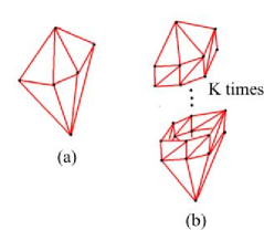
Figure 18: Diamond type graphs. In fig. (b) there are $K$ layers of the sequences of rectangles constructed from couples of triangles.

For such graphs:

$$C_{2}(M)=2\,\frac{(M/2)^{2}}{2}+M\,\frac{4^{2}}{2}-3\,M$$

and hence $C_{2}(M)/M^{2}\to 1/4$ in the limit $M\to\infty$ and the $C_{2}$ term survives the limit. These considerations mean that the limit (10) depends on actual choices of the graphs in the sequence.

However, if we consider the graphs of type 18 (b) with fixed $K$ then:

$$C_{2}(M)=\frac{2}{2}\,\left(\frac{M}{2(K+1)}\right)^{2}+\frac{M}{K+1}\frac{5^{2}}{2}+\left(\frac{M}{2}-2-\frac{M}{K+1}\right)\,\frac{6^{2}}{2}-3\,M.$$

Hence, if $M\to\infty$ and $K$ is fixed then

$$\frac{C_{2}(M)}{M^{2}}\to\frac{1}{4(K+1)^{2}}$$

and again the $C_{2}$ term survives the limit. Note, however, that for fixed $K$ the number of triangles meeting at the poles of the diamond 18 (b) is of the order of $M$.

Now, if we take the limit $K\to\infty$ then $C_{2}(M)/M^{2}\to 0$ and the number of triangles meeting at the poles of the diamond is suppressed in comparison with respect to $M$. Hence, to avoid the complication with the dependence of the limit $M\to\infty$ on the choice of graphs in eq.(10)  we have to take such graphs in which the number of triangles meeting at each vertex is suppressed in comparison with $M$. Then $C_{2}(M)$ does not survive the limit $M\to\infty$ and the eq.(10)  does not depend on the choices of the graphs in the sequence. Then $C_{1}(M)/M^{2}\to\mathbb{C}_{M}^{2}/M^{2}\to 1/2!$.

Presented here considerations are valid for graphs of any genera, i.e. $C_{2}$ and $C_{3}$ terms vanish for any genera. Similar but a little more tedious calculation we performed for the $\hat{B}^{3}$ terms. It appears that the only surviving term is (if $n_{max}(M)/M\to 0$ as $M\to\infty$):

$$\frac{1}{3!}\,B^{j^{(1)}_{1}\,j^{(1)}_{2}\,j^{(1)}_{3}}\,B^{j^{(2)}_{1}\,j^{(2)}_{2}\,j^{(2)}_{3}}B^{j^{(3)}_{1}\,j^{(3)}_{2}\,j^{(3)}_{3}}\,I^{g}_{j^{(1)}_{3}\,j^{(1)}_{2}\,j^{(1)}_{1}\left|j^{(2)}_{3}\,j^{(2)}_{2}\,j^{(2)}_{1}\right|j^{(3)}_{3}\,j^{(3)}_{2}\,j^{(3)}_{1}}.$$

As well we expect similar story to happen for higher orders in powers of $\hat{B}$. In fact, consider $F$ matrices $\hat{B}$ spread over a graph with $M$ faces. Then on general grounds we can expect that if $M\to\infty$ configurations where $\hat{B}$’s meet each other are suppressed (under the conditions listed below eq.(10) ) in comparison with the one where they are separated. As the result we obtain eq.(14) .

References

- [1] V. Dolotin, arXiv:math.gt/9904026.
- [2] Yu.Chernyakov and V.Dolotin, math/0501206.
- [3] M. Fukuma, S. Hosono and H. Kawai, Commun. Math. Phys. 161, 157 (1994) [arXiv:hep-th/9212154].
- [4] E. Verlinde, Nucl. Phys. B 300, 360 (1988).
- [5] V. G. Turaev and O. Y. Viro, Topology 31, 865 (1992).
- [6] A. Gerasimov, A. Morozov and K. Selivanov, Int. J. Mod. Phys. A 16, 1531 (2001) [arXiv:hep-th/0005053].
- [7] E. T. Akhmedov, JETP Lett. 80, 218 (2004) [Pisma Zh. Eksp. Teor. Fiz. 80, 247 (2004)] [arXiv:hep-th/0407018].
- [8] E. T. Akhmedov, arXiv:hep-th/0502174.