ROM2F-05/06                                                                                                        hep-th/0503204

Abstract

This Thesis discusses a number of issues related to the problem of tadpoles and vacuum redefinitions that the breaking of supersymmetry brings about in String Theory. The idea pursued here is to try to formulate the theory in a “wrong” vacuum (the vacuum that one naively identifies prior to the redefinitions) and, gaining some intuition from some simpler field theory settings, try to set up a calculational scheme for vacuum redefinitions in String Theory. This requires in general complicated resummations, but some simpler cases can be identified. This is true, in principle, for models with fluxes, where tadpoles can be perturbatively small, and for the one-loop threshold corrections, that in a large class of models (without rotated branes) remain finite even in the presence of tadpoles. The contents of the Thesis elaborate on those of hep-th/0410101, but include a number of additions, related to the explicit study of a quartic potential in Field Theory, where some subtleties were previously overlooked, and to the explicit evaluation of the one-loop threshold corrections for a number of string models with broken supersymmetry.

( March , 2005 )

UNIVERSITÀ DEGLI STUDI DI ROMA
                  “TOR VERGATA”

Issues on tadpoles and vacuum redefinitions in String Theory

Candidato
Marco Nicolosi

Relatore
Prof. Augusto Sagnotti

Coordinatore del dottorato
Prof. Piergiorgio Picozza

Ciclo XVII

Anno Accademico 2004-2005

Introduction

The Standard Model and some of its problems

Quantum Field Theory is a powerful tool and an extremely appealing theoretical framework to explain the physics of elementary particles and their interactions. The Standard Model describes such interactions in terms of Yang-Mills gauge theories. The gauge group $SU(3)\times SU(2)\times U(1)$ reflects the presence of three fundamental forces: electromagnetism, the weak interaction, and the strong interaction. All these forces are mediated by spin-one bosons, but they have a very different behavior due to their abelian or non-abelian nature.

In electromagnetism the gauge bosons are uncharged and thus a test charge in vacuum can be only affected by the creation and annihilation of virtual particle-antiparticle pairs around it and these quantum fluctuations effectively screens its charge. On the other hand, for the other two interactions there is a further effect of anti-screening due to radiation of virtual gauge bosons that now are charged, and this second effect is the one that dominates at short distances in the strong interactions. Its consequence is the asymptotic freedom at high energies, well seen in deep inelastic scattering experiments, and more indirectly the confinement of quarks at low energies, that explains why there no free colored particles (the particles that feel the strong interactions) are seen in nature. The weak interactions should have the same nature (and therefore the same infrared behavior) as the strong ones, but a mechanism of symmetry breaking that leaves a residual scalar boson, the Higgs boson, gives mass to two of the gauge-bosons mediating the interaction, and makes its intensity effectively weak at energy scales lower than $M_{W}\simeq 100GeV$.

The picture is completed adding the matter that is given by leptons, that only feel electro-weak interactions, and quarks, that feel also the strong interactions. Matter is arranged in three different generations. The peculiar feature of the Standard Model, that makes it consistent and predictive, is its renormalizability. And indeed the Standard Model was tested with great precision up to the scale of fractions of a $TeV$. However, in spite of the agreement with particle experiments and of the number of successes collected by Standard Model, this theory does not give a fully satisfactory setting from a conceptual point of view.

The first problem that arises is related to the huge number of free parameters from which the Standard Model depends, like the gauge couplings, the Yukawa couplings, the mixing angles in the weak interactions, to mention some of them. The point is that there is no theoretical principle to fix their values at a certain scale, but they have to be tuned from experiments.

The last force to consider in nature is gravity. This force is extremely weak with respect to the other forces, but contrary to them, it is purely attractive and hence it dominates at large-scales in the universe. At low energies, the dynamics of gravity is described in geometrical terms by General Relativity.

In analogy with the fine-structure constant $\alpha=q^{2}/\hbar c$ that weights the Coulomb interaction, one can define a dimensionless coupling for the gravitation interaction of the form $\alpha_{G}=G_{N}E^{2}/\hbar c^{5}$, where $G_{N}$ is the Newton constant. In units of $\hbar=c=1$, one can see that $\alpha_{G}\sim 1$ for $E\sim 1/\sqrt{G_{N}}=M_{Pl}$, where the Planck mass is $M_{Pl}\sim 10^{19}GeV$. So we see that the gravitational interaction becomes relevant at the Planck scale, and therefore one should try to account for quantum corrections. If the exchange of a graviton between two particles corresponds to an amplitude proportional to $E^{2}/M^{2}_{Pl}$, the exchange of two gravitons is proportional to

$$\frac{1}{M_{Pl}^{4}}\int_{0}^{\Lambda}E^{3}dE\sim\frac{\Lambda^{4}}{M_{Pl}^{4}}\ ,$$ (1)

that is strongly divergent in the ultraviolet. And the situation becomes worse and worse if one considers the successive orders in perturbation theory: this is the problem of the short distance divergences in quantum gravity, that makes the theory non renormalizable. Of course a solution could be that quantum gravity has a non-trivial ultraviolet fixed-point, meaning that the divergences are only an artifact of the perturbative expansion in powers of the coupling and therefore they cancel if the theory is treated exactly, but to date it is not known whether this is the case. The other possibility is that at the Planck scale there is new physics. The situation would then be like with the Fermi theory of weak interaction, where the divergences at energy greater then the electro-weak scale, due to the point-like nature of the interaction in the effective theory, are the signal of new physics at such scale, and in particular of the existence of an intermediate gauge boson. In the same way, it is very reasonable and attractive to think that the theory of gravity be the infrared limit of a more general theory, and that the divergences of quantum gravity, actually due to the short distances behavior of the interaction, could be eliminated smearing the interaction over space-time.

But the problem of the ultraviolet behavior of quantum gravity is not the only one, when one considers all the forces in nature. The first strangeness that it is possible to notice is the existence of numbers that differ by many orders of magnitude. This problem is known as the hierarchy problem. For example, between the electro-weak scale, the typical scale in the Standard Model, and the Planck scale, whose squared inverse essentially weighs the gravitational interaction, there are $17$ orders of magnitude. Not only, the other fundamental scale in gravity, $\Lambda^{1/4}\sim 10^{-13}GeV$, where $\Lambda$ is the cosmological constant, is also very small if compared with the electro-weak energy $E_{W}\sim 100GeV$. Moreover, there are other hierarchy differences in the parameters of the Standard Model, for instance in the fermion masses. Differences of many orders of magnitude seem very unnatural, especially considering that quantum corrections should make such values extremely unstable. Supersymmetry, introducing bosonic and fermionic particles degenerate in mass, stabilizes the hierarchy but does not give any explanation of such differences.

The last problem that we want to mention is the cosmological constant problem [1]. One can naturally associate the cosmological constant to the average curvature of the universe, and of course the curvature is related to its vacuum energy density. Therefore, one could try to estimate such a density from the microscopic point of view $\rho_{micro}$, and compare it with the macroscopic value $\rho_{macro}$, obtained by astrophysical observations. The first estimate is provided in Quantum Filed Theory considering the zero-point energy of the particles in nature. For example at the Planck scale $\rho_{micro}\sim M_{Pl}^{4}c^{5}/\hbar^{3}$. On the other hand, from a simple dimensional analysis, the macroscopic density can be expressed in terms of the Hubble constant $H$ through the relation $\rho_{macro}\sim H^{2}c^{2}/G_{N}$. The point is that the theoretical estimate is $120$ orders of magnitude greater than the observed value. Surely, supersymmetry can improve matters. Fermions and bosons contribute to the vacuum energy with an opposite sign and so a supersymmetric theory would give a vanishing result for $\rho_{micro}$. One can break supersymmetry at the scale of the Standard Model with $E_{breaking}\sim TeV$ and considering $\rho_{micro}\sim E_{breaking}^{4}/\hbar^{3}c^{3}$, but there is an improvement of only $30$ orders of magnitudes. In spite of all the attempts to solve this great mismatch, the cosmological constant problem up to date remains essentially unsolved.

The birth of String Theory and the Dual Models

In the sixties physicists were facing the problem of the huge zoology of hadronic resonances that the high energy experiments were revealing. A fact was that the spin $J$ and the mass $m^{2}$ of such resonances appeared to be related linearly trough the simple relation $m^{2}=J/\alpha^{\prime}$, checked up to $J=11/2$, where $\alpha^{\prime}\sim 1GeV^{-2}$ became known as the Regge slope. Another key ingredient of the hadronic scattering amplitudes was the symmetry under the cyclic permutation of the external particles. Considering the scattering of two hadrons (1,2) going into two other hadrons (3,4) and defining the Mandelstam variables as usual

$$s=-(p_{1}+p_{2})^{2}\ ,\qquad t=-(p_{2}+p_{3})^{2}\ ,\qquad u=-(p_{1}+p_{3})^{2}\ ,$$ (2)

the symmetry under the cyclic permutation $(1234)\rightarrow(2341)$ reflects itself in the planar duality under the interchange of $s$ with $t$. On the other hand, if one attempts to write the interaction due to the exchange of an hadronic resonance of spin $J>1$ and mass $m^{2}_{J}$, one should obtain a vary bad ultraviolet behavior with increasing $J$. In fact, the corresponding scattering amplitude in the $t$-channel at high energy would be proportional to

$$A_{J}(s,t)\sim\frac{(-s)^{J}}{t-m^{2}_{J}}\ .$$ (3)

It was Veneziano [2] that in 1968 wrote a formula for the scattering amplitude obeying planar duality and with an ultraviolet behavior far softer then any local quantum field theory amplitude,

$$A(s,t)\ =\ \frac{\Gamma(-\alpha(s))\Gamma(-\alpha(t))}{\Gamma(-\alpha(s)-\alpha(t))}\ ,$$ (4)

where $\Gamma$ is the usual $\Gamma$-function, and $\alpha(s)=\alpha(0)+\alpha^{\prime}s$. The Veneziano amplitude has poles corresponding to the exchange of an infinite number of resonances of masses $m^{2}=n-\alpha(0)/\alpha^{\prime}$, and it is just the sum over all these exchanges that gives to the dual amplitude its soft behavior at high energy.

In spite of its beauty and elegance, the Veneziano formula soon revealed not suitable to describe the hadronic interactions, since it predicts a decrease of the scattering amplitudes with energy that is too fast with respect to the indications of the experimental data. The Veneziano formula and its generalization due to Shapiro and Virasoro [3] to a non-planar duality (symmetry with respect to the exchange of each pair of the variables $s$, $t$, $u$), were instead associated in a natural way to the scattering amplitudes respectively of open and closed strings. In particular, the infinite number of poles of such amplitudes corresponding to the exchange of particles of higher spin and mass can be read as a manifestation of the infinite vibrational modes of a string. One of the peculiar features of the closed string is that it contains a massless mode of spin 2, that its low-energy interactions associate naturally to the graviton. Hence a theory of closed strings seems to be a possible candidate to describe quantum gravity without the usual pathologies at short distances, given the soft behavior in the ultraviolet regime of the interactions in the dual models. The Regge slope in this case has to be identified with the characteristic scale in quantum gravity, the Planck scale, $\sqrt{\alpha^{\prime}}\sim 10^{-33}cm$. A simple argument to understand why the interaction between two strings has such a good ultraviolet behavior is to consider that in the scattering the interaction is spread along a fraction of the length of the strings. Hence, only a fraction of the total energy is really involved in the interaction, and the coupling $\alpha_{G}$ is effectively replaced by

$$\alpha_{eff}\ =\frac{G_{N}E^{2}}{\hbar c^{5}}\ \left(\frac{\hbar c}{E\ell_{s}}\right)^{2}\ ,$$ (5)

where $\ell_{s}=\sqrt{\alpha^{\prime}}$ is the length of the string. One can observe that the bad dependence of $E^{2}$ is thus cancelled in $\alpha_{eff}$. On the other hand, an open string has in its spectrum a massless mode of spin one, that can be associated to a gauge vector. Therefore String Theory seems also to furnish a way to unify all the forces in nature, giving one and the same origin for gravity and gauge interactions.

At the beginning in the Veneziano model, String Theory contained only bosonic degrees of freedom. Moreover it predicted the existence of a tachyon in its spectrum. It was thanks to the work of Neveu, Schwarz and Ramond [4] that it was understood how to include fermions in the theory. Moreover, the work of Gliozzi, Scherk and Olive [5] was fundamental to understand how to obtain supersymmetric spectra, projecting away also the tachyon. Another peculiarity of String Theory is that quantum consistency requires additional spatial dimensions. The dimensionality of space-time is $D=26$ for the bosonic String and $D=10$ for the Superstring. This feature of String Theory of course is very appealing and elegant from a conceptual point of view (it connects to the original work of Kaluza and Klein that unified the description of a graviton, a photon and a massless scalar field in $D=4$ starting from a theory of pure gravity in $D=5$), but provides that the additional dimensions be compactified on some internal manifold, to recover the $3+1$ dimensions to which we are used. On the one hand, choosing different internal manifolds one can obtain different four dimensional low-energy effective field theories. Moreover, one has the possibility of choosing some of the internal radii large enough, and this is important for trying to solve the hierarchy problem. By suitable compactifications it is also possible to break supersymmetry. All these possibilities are surely key ingredients that compactifications offer to String Theory, but on the other hand the presence of the additional dimensions is a major problem for the predictivity of the parameters of the four-dimensional world. We will come back on this issue in the following.

M-theory scenario and dualities

Today we know that there are five different supersymmetric ten-dimensional String Models. They are Type IIA, Type IIB, Type I $SO(32)$, heterotic $SO(32)$ (or HO) and heterotic $E_{8}\times E_{8}$ (or HE). A lot of effort was devoted during the last decade in the attempt to unify them. It was finally understood that all these models can be regarded as different limits of a unique theory at 11 dimensions, commonly called M-theory [6]. Moreover, all these theories are related to one another by some transformations known as dualities. Surely a string has an infinite number of vibrational modes corresponding to particles of higher and higher masses. Such masses are naturally of the order of the Planck scale, but one can consider only the massless sector. In other words, one can think to make an expansion in powers of the string length $\ell_{s}=\sqrt{\alpha^{\prime}}$, recovering the point-particle low-energy effective field theory in the $\ell_{s}\to 0$ limit. At this level what we find are some supersymmetric generalizations of General Relativity known as supergravity theories. In ten dimensions exist three different supersymmetric extensions of gravity: the Type IIA supergravity, that has supersymmetry ${\mathcal{N}}=(1,1)$, the Type IIB supergravity, with ${\mathcal{N}}=(2,0)$ and the Type I supergravity, with supersymmetry ${\mathcal{N}}=(1,0)$, but all of them have a common sector consisting in a graviton $G_{\mu\nu}$, a dilaton $\phi$ and an antisymmetric two-tensor,a 2-form, $B_{\mu\nu}$. The dynamics of such universal sector is governed by the effective action

$$S_{eff}\ =\ \frac{1}{2k_{10}^{2}}\int d^{10}x\sqrt{-{\rm det}G}e^{-2\phi}\left(R+4\partial_{\mu}\phi\partial^{\mu}\phi-\frac{1}{12}H^{2}\right)\ ,$$ (6)

where $R$ is the curvature scalar, $k_{10}^{2}$ is related to the ten-dimensional Newton constant, and $H_{\mu\nu\rho}$ is the field strength of the 2-form.

The dilaton plays in String Theory a crucial role, since it weighs the perturbative expansion. Moreover, its vacuum expectation value $\langle\phi\rangle$, is a first example of a modulus a free dynamical parameter from which the theory depends. We want to stress that there is no potential to give a vacuum value to the dilaton, and thus its expectation value remains undetermined. Hence in ten dimensions one has actually a one-parameter family of vacua labelled by the arbitrary expectation value of the dilaton. Notice that the coupling constant $k_{10}^{2}$ in the effective action (6) is not really a free parameter of the theory. In fact, introducing the string coupling constant $g_{s}=e^{\langle\phi\rangle}$, one can see that a change of $k_{10}^{2}$ can be reabsorbed by a shift to the vacuum expectation value of the dilaton.

After this digression on the role of dilaton, we can come back to the dualities. The Type IIA and IIB superstring theories contain only oriented closed strings and have as low-energy effective field theories respectively the ten-dimensional supergravities of types IIA and IIB. On the other hand, the Type I superstring has unoriented closed and open strings, and thus we expect that it describe at same time gravity and gauge interactions. And in fact its low-energy behavior is governed by the Type I supergravity together with the supersymmetric generalization of a Yang-Mills theory with gauge group $SO(32)$. The Heterotic String is a theory of closed strings. Now a closed string has left and right moving modes and they are independent, and so one can consider the right modes of the usual superstring in ten-dimensions together with the left modes of the bosonic string compactified from $D=26$ to $D=10$. Notice that the compactification introduces in a natural way the internal degrees of freedom of a gauge theory without the need to introduce open strings. The resulting theories are supersymmetric and free from tachyons. Moreover, string consistency conditions fix the choice of the internal lattice to only two possibilities: the first one corresponds to the roots of the lattice of $E_{8}\times E_{8}$, while the second one to the roots of $SO(32)$. Hence, in the low-energy limit, the two heterotic strings give the usual Type I supergravity coupled to a Super Yang-Mills theory with gauge group $E_{8}\times E_{8}$ or $SO(32)$. There exist also other non supersymmetric ten-dimensional heterotic models corresponding to different projection of the spectrum. Perhaps the most interesting, not supersymmetric but free from tachyons, is the $SO(16)\times SO(16)$ model.

At the end of the seventies, Cremmer, Julia and Scherk found the unique supergravity theory in eleven dimensions. Its bosonic spectrum contains the metric and a 3-form $A_{3}$ whose dynamics is given by the action

$$S_{11}\ =\ \frac{1}{2k^{2}_{11}}\int d^{11}x\sqrt{-{\rm det}G}\ \left(R-\frac{1}{24}F_{IJKL}F^{IJKL}\right)\ -\ \frac{\sqrt{2}}{k^{2}_{11}}\int A_{3}\wedge F_{4}\wedge F_{4}\ ,$$ (7)

where $k_{11}$ is related to the eleven dimensional Newton constant, and $F_{4}=6dA_{3}$ is the field strength of the 3-form. Notice that, in net contrast with the ten-dimensional supergravities, here the spectrum does not contain any 2-form.

However compactifying the eleventh dimension on a circle one recovers the ten-dimensional Type IIA supergravity. And this is not all. If one compactifies the eleven-dimensional supergravity on a segment $S^{1}/{\mathbb{Z}}_{2}$, one recovers the low-energy theory of the heterotic $E_{8}\times E_{8}$ string [7]. At this point it is quite natural to think that, just like all ten-dimensional supergravities are low-energy limits of the corresponding superstring theories, so even the eleven-dimensional supergravity can be regarded as the low-energy limit of a more fundamental theory, that is commonly called M-theory [6]. What is M-theory up to date is not known. In particular, we do not know what are its fundamental degrees of freedom. Surely what we can say is that it is not a theory of strings. In fact, as we already said, all ten-dimensional supergravity theories contain in their spectrum a 2-form. Now a two-form has just the right tensorial structure to describe the potential for a one-dimensional object (a string), just like in the usual case the potential for a point charge is a vector. Therefore the presence of the 2-form in the spectrum is a clear signal that the dynamics is described by strings, while its absence in the spectrum of the eleven-dimensional supergravity reveals that M-theory is not related to strings.

Up to now we discussed how to recover the Type IIA and the Heterotic $E_{8}\times E_{8}$ models from the mysterious M-theory. But the surprises are not finished. In fact, the other ten-dimensional models are also related to one another through some transformations known as dualities. In general a duality is an invertible map that connects the states of a theory to the ones of another theory (or of the same theory) preserving interactions and symmetries. The importance and utility of a duality can be appreciated already in Quantum Field Theory, where generally one makes the perturbative expansion in powers of $\hbar$. The point is that not all quantities can be described in terms of a perturbative series, and a duality can help because it allows to see the same phenomenon in another description. A case of particular interest is provided by a duality that maps the perturbative region of a theory into the non-perturbative region of the same theory. This is the case of the $S$-duality [8] in String Theory.

Figure 1: Dualities between different ten-dimensional String Theories.

Such duality inverts the string coupling constant

$$S\ :\ g_{s}\ \longleftrightarrow\ \frac{1}{g_{s}}\ ,$$ (8)

and, as can be seen from the figure1, maps the $SO(32)$ Heterotic String to the Type I $SO(32)$ String. More precisely, $S$-duality identifies the weak coupling limit of one theory with the strong limit of the other. Moreover, the Type IIB model is self-dual. The weak-strong coupling $S$-duality is manifest in the low-energy effective field theories, but really the duality, being non-perturbative, remains only a conjecture, as the strong coupling limit of String Theory is not fully under control. However, up to date, all non perturbative tests revealed no discrepancy with the conjecture of duality.

A crucial step in the understanding of the $S$-duality is the existence in the spectra of the various string models of extended objects with $p$ spatial dimensions, whose presence is fundamental for the right counting and the matching of the degrees of freedom after a non perturbative duality is performed. These objects corresponds to solitonic configurations with tension proportional to the inverse of the string coupling constant (in net contrast with the usual case in Field Theory where the tension is proportional to the squared inverse of the coupling), and are mapped by an $S$-duality in the usual perturbative string states. They are known as $p$-branes and if originally they appeared as classical supergravity solutions, then it was realized that some of these objects, known as D$p$-branes [9], can be thought as topological defects where open strings terminate, with Dirichlet boundary conditions in the directions orthogonal to them and Neumann ones in the parallel directions. A D-brane is characterized by its tension and by a charge that is defined by the coupling of the brane to a corresponding tensor potential. Together with D-branes, one can also define antibranes, $\bar{\rm D}$-branes, that are characterized by the same tension but by a reversed charge.

Another important duality, that in contrast with the previous one is perturbative, is the $T$-duality between the Type IIA and Type IIB theories or between the Heterotic $E_{8}\times E_{8}$ and $SO(32)$ theories. In particular, a $T$-duality identifies one theory compactified on a circle of radius $R$ with the other theory compactified on a circle of radius $1/R$. A peculiar feature of $T$-duality is that it interchanges Neumann and Dirichlet boundary conditions [10, 11, 12], and thus it changes the dimensionality of a D-brane. And indeed the content of D$p$-branes of Type IIA and Type IIB models are just the right one to respect the T-duality relating them (D$p$-branes with $p$ odd for Type IIB and $p$ even for Type IIA).

The last link we need to unify all the five ten-dimensional superstring models is the orientifold projection $\Omega$ [13] that connects the Type IIB String with the Type I String. $\Omega$ exchanges the left and right modes of a closed string, and the Type I String is obtained identifying the left and right modes of Type IIB. The fixed points of such projection correspond to some extended non dynamical space-time objects known as the orientifold-planes or briefly O-planes. In contrast with a D-brane, whose tension is always positive, an O-plane can also have a negative tension. Moreover, like a D-brane, an O-plane carries a charge with respect to some tensor potential.

Now the hexagon of dualities is closed (see figure1) and what we learn is that in spite of their apparent differences, all the ten-dimensional superstring theories can be thought of really as different limits in a certain parameter space of a unique underlying theory that is identified with the M-theory. Notice that in this appealing picture the fact that the eleven-dimensional supergravity is unique is very compelling from the unification point of view.

A crucial matter that we have to stress before closing this discussion is the consistency of all these ten-dimensional Superstring Theories, and in particular the absence of anomalies in their spectra. Anomalies arise already in Field Theory, and are quantum violations of classical symmetries. The violation of a global symmetry is not dangerous and often can be useful from a phenomenological point of view. For example, in the theory of the strong interaction with massless quarks, the quantum violation of the classical scale invariance is a mechanism that gives mass to the hadrons. On the other hand a violation of a local symmetry, like the gauge symmetry in a Yang-Mills theory or the invariance under diffeomorphisms in General Relativity, is a real problem since the unphysical longitudinal degrees of freedom no longer decouple, and as a consequence the theory loses its unitarity. Therefore, the cancellation of all (gauge, gravitational, mixed)-anomalies is a fundamental property to verify in String Theory. The first type of cancellation of anomalies in String Theory is achieved imposing the tadpole condition in the Ramond-Ramond (R-R) sector. We will come back to the issue of tadpoles in the following, but for the moment what we really need to know is that such condition from the space-time point of view corresponds to imposing that the Faraday-lines emitted by the branes present in the model be absorbed by the O-planes, or in other words that the compactified space-time be globally neutral. Such a condition fix also the gauge group for the Type I models. The other anomalies arising in String Theory from the so called non-planar diagrams are cancelled thanks to a mechanism due to Green and Schwarz [14]. The anomaly of the one-loop hexagon-diagram, the analog of the triangle-diagram in four dimensions that one meets in gauge theory, is exactly cancelled by a tree-level diagram in which the 2-form propagates. This mechanism works in all the ten-dimensional theories we saw (the Type IIA is not anomalous because is not chiral). The mechanism of Green and Schwarz can be generalized to the case of several 2-forms [15] and is at the heart of the consistency of string models.

Compactifications and supersymmetry breaking

Up to now we presented some arguments why String Theory should be consider a good candidate for quantum gravity. Moreover, we saw that all the consistent supersymmetric ten-dimensional models are really dual one to the other and that all of them can be linked to a unique eleven-dimensional theory. Finally, String Theory describes together gravity and gauge interactions, giving a concrete setting for unifying in a consistent fashion all the forces of the Standard Model with Quantum Gravity. The following step we need to recover our four dimensional world is a closer look at the compactification of the six additional dimensions on an internal manifold. A single string state gives an infinite tower of massive excitations with masses that are related to the inverse of the internal dimensions, but from the low-energy point of view one can effectively think that all the massive recurrences disentangle if the typical size of the internal volume is small enough. The other key ingredient in order to get a realistic four-dimensional physics is supersymmetry breaking, that really can be also related to the issue of compactification. We will therefore review these two arguments together, showing also how the presence of D-branes can provide some new natural settings to break supersymmetry.

The simplest way to realize compactifications in String Theory is to choose as internal manifold a torus. This follows the lines traced by Kaluza and Klein, but a closed string offers more possibilities with respect to a point particle, since a string can also wrap around a compact dimension. Another interesting setting is provided by orbifold [16] compactifications, obtained identifying points of a certain internal manifold under the action of a discrete group defined on it. Such identifications in general leave a number of fixed points where the Field Theory would be singular but String Theory is well defined on it. A further interesting and elegant setting for compactification is furnished by Calabi-Yau spaces, that in contrast with the orbifold compactifications are smooth manifolds and in suitable limits reduce to orbifolds that are exactly solvable in String Theory. A Calabi-Yau $n$-fold is a complex manifold on which a Ricci-flat Kähler metric can be defined. As a consequence a non trivial $SU(n)$ holonomy group emerges that in turn is responsible for supersymmetry breaking on such spaces. For instance, a six-dimensional Calabi-Yau with holonomy group $SU(3)$ preserves only ${\mathcal{N}}=1$ supersymmetry. Different $SU(3)$ Calabi-Yau manifolds can be recovered blowing up in different ways the fixed points of the orbifold $T^{6}/\mathbb{Z}_{3}$. Another interesting example of a Calabi-Yau manifold is provided by the space $K3$ [17], with holonomy $SU(2)$, that gives a four-dimensional ${\cal N}=2$ supersymmetry and in a suitable limit reduces to the orbifold $T^{4}/{\mathbb{Z}}_{2}$.

Supersymmetry breaking can be obtained in standard toroidal or orbifold compactifications. The important thing to notice is that in the first case supersymmetry is broken at a scale fixed by the radius of the internal manifold. In fact, one can generalize the Scherk-Schwarz [18, 19] mechanism to String Theory, for instance giving periodic boundary condition on a circle to bosons and antiperiodic conditions to fermions. In this way the masses of the Kaluza-Klein excitations are proportional to $n/R$ for bosons and $(n+1/2)/R$ for fermions, and thus the gauginos or gravitinos are lifted in mass and supersymmetry is broken at the scale $1/R$. This way to break supersymmetry is like a spontaneous breaking and in the limit of decompactification one recovers all the original supersymmetry. This fact is in net contrast with the case of breaking through orbifold compactification, where the breaking is obtained projecting away some states, and after the orbifolding no trace of the original supersymmetry remains. On the other hand, it would be interesting to break supersymmetry at a scale which is independent from $R$, for example at the string scale, that in some recent models requiring large extra-dimensions, can even be of the order of $TeV$.

A new interesting phenomenon happens when one breaks supersymmetry by toroidal compactification in the presence of D-branes [20, 21]. So let us consider the case of some branes parallel to the direction of breaking. This case is called usually “Scherk-Schwarz breaking”, and supersymmetry is broken both in the bulk (closed sector) and on the branes (open sector). The spectrum is a deformation of a supersymmetric one that can be recovered in the decompactification limit. Something new happens if the direction of breaking is orthogonal to the branes (really we are thinking in a T-dual picture). In this case, at least at the massless level, supersymmetry is preserved at tree-level on the branes. This phenomenon is commonly called “brane supersymmetry”, and indeed at tree level the gaugino does not take any mass. Really supersymmetry breaking on the branes is mediated by radiative corrections due to the gravitational interactions, and so also the gaugino eventually gets a mass that with respect to the one of gravitino is suppressed by the Planck mass, being a quantum effect. This phenomenon however has not been fully studied to date. In contrast with the previous case one can break supersymmetry on the branes, and there are essentially two ways to do that. The first one is provided by models that require configurations with the simultaneous presence of branes and antibranes of different types [21]. In this case the closed sector is supersymmetric, but is generally different from the standard supersymmetric one, while supersymmetry is broken at the string scale on the open sector, as branes and antibranes preserve different halves of the original supersymmetry. This kind of configurations, however is classically stable and free of tachyons. The second one is obtained deforming a supersymmetric open spectrum with a system of separated brane-antibrane pairs of the same type. Such a configuration is unstable due the attractive force between branes and antibranes and a tachyon develops if their distance if small. The last known way to break supersymmetry in String Theory is with intersecting D-branes [22], that in a T-dual picture corresponds to turning on constant magnetic fields on the internal manifold [23]. A very appealing feature of this kind of breaking is that chiral fermions in different generations can live at the intersections of the branes.

Directly related to the issue of dimensional reduction and supersymmetry breaking are two of the greatest problems of String Theory. A common problem one has to face in String Theory when one performs a reduction from the ten-dimensional world to the four-dimensional one is the emergence of quantities that remain arbitrary. These are the moduli, an example of which we already met in the vacuum expectation value of the dilaton. At the beginning of this Introduction we mentioned the problem of the large number of free parameters present in the Standard Model. Of course it would be great to get some predictions on them from String Theory, but this is not what happens. The four-dimensional low-energy parameters after the reduction from ten-dimensions depend on some moduli, like for example the size and shape of the extra dimensions, and their predictivity is related to the predictivity of such moduli. Now in gravity there is no global minimum principle to select a certain configuration energetically more stable than another one, and so really the moduli remain arbitrary. This problem is known as the moduli problem, and up to date represents the greatest obstacle for the predictivity of the Standard Model parameters from String Theory. Therefore, in spite of a unique (thanks to dualities) ten-dimensional theory, in four dimensions we have typically a continuum of vacua labelled by the expectation values of such moduli. Really the moduli problem is always associated to supersymmetric configurations. And in fact supersymmetry if on the one hand stabilizes the space-time geometry, on the other hand makes the moduli arbitrary in perturbation theory (this is not true non perturbatively for ${\mathcal{N}}=1$). Of course, one has to break supersymmetry at a certain scale to recover the observed physics, but in that case the arising quantum fluctuations are not under control, and moreover some infrared divergences due to the propagation of massless states going into the vacuum can affect the string computations. These divergences typically arise when one breaks supersymmetry, and are related to the presence of uncancelled Neveu-Schwarz Neveu-Schwarz (NS-NS) tadpoles. Physically, their emergence means that the Minkowski background around which one quantizes the theory after supersymmetry breaking is no more a real vacuum, and has to be corrected in order to define reliable quantities. This is the problem of the vacuum redefinition in String Theory with broken supersymmetry and we will deal at length with this issue in the following, since it is the main theme of this Thesis. For the moment, let us return to the moduli problem.

An important attempt to stabilize the moduli is provided by compactifications with non trivial internal fluxes [24]. After supersymmetry breaking a modulus takes some vacuum expectation value but in general, for the technical reasons we already stressed, it is not possible to compute it. In contrast with this fact, if one turns on some background potentials on the internal manifold, a low-energy effective potential arises and many of the moduli are frozen. The nice thing to underline in the presence of fluxes is the possibility to compute the effective potential. Really what one can do for general Calabi-Yau compactifications is to build an approximate expansion of the potential around its extrema, but there are also simple orbifold compactifications in which the potential for some moduli is known globally. Moreover, playing with the internal fluxes, one can also stabilize most of the moduli without breaking supersymmetry.

Brane-worlds

A very interesting scenario that has been developed in the last years is provided by the so called brane-worlds [26, 27]. As we already said, the tension of a brane scales as the inverse of the string coupling constant, and so it seems to be like a rigid wall at low energy, but of course its dynamics can be described by the open strings terminating on it. In fact, the low-energy open string fluctuations orthogonal to the branes correspond to the oscillations of the brane from its equilibrium position and from the brane point of view such modes are effectively seen as scalar fields arising as Goldstone bosons of the translational symmetry of the vacuum broken by the presence of the brane. In the same way, the fermions living on the branes can be seen as goldstinos arising after the breaking of supersymmetry introduced by the presence of the brane. On the other hand, the parallel fluctuations of a string terminating on the brane describe at low energy a $U(1)$ gauge boson. A supersymmetric D$p$-brane is really a BPS state, meaning that it preserves only half of the total supersymmetry of Type II vacua, and that its tension and charge are equal. This implies that between two parallel branes the gravitational attraction is compensated by the Coulomb repulsion and no net force remains. So one has the possibility to superpose some branes, let say $N$, with the consequence of enhancing the gauge symmetry to $U(N)$ due to the fact that now an open string has $N\times N$ ways to start and end on the $N$ D-branes. In other words a stack of $N$ coincident D-branes gives the possibility to realize non abelian interactions for the open strings, while their displacement can be seen as a sort of spontaneous symmetry breaking preserving the total rank. A nice thing to notice is that while the low-energy dynamics of the gauge filed living on the branes is the usual one described by Yang-Mills theory, the higher energy string corrections remove the usual divergence at $r\to 0$ of the Coulomb interaction between point charges. And in fact the low-energy effective action for the open string modes, at least in the abelian case, is given by the Born-Infeld action [29]. For example, in the case of a static electric field, the usual power law of the Coulomb interaction $1/r^{2}$ is replaced by $1/\sqrt{r^{4}+(2\pi\alpha^{\prime})^{2}}$ and so we see that the string once more time regulates the short-distance divergence.

At this point we saw that stacks of D-branes describe non abelian gauge groups and that the displacement of D-branes is responsible for gauge symmetry breaking. But with branes one can obtain more. And in fact, as already stressed, the intersection of D-branes can lead to chiral fermions coming from the open strings stretched between them (really, considering the low lying modes, these chiral fermions live in the intersection volume of the branes). The interesting possibility provided by this setting is that chiral fermions are obtained in a number of replicas giving a realistic set up in which one can try to reproduce the matter fields (and the gauge group) of the Standard Model [28]. A simple example to understand the origin of the matter replication is given by a configuration with two stacks of D6-branes that intersect in a four-dimensional volume. Now we have to think the other dimensions of the branes as wrapped around some 3-cycles of an internal compact six-dimensional space. Two such 3-cycles can intersect several times in the internal manifold, thus leading to replicas of the chiral matter living at the four-dimensional intersection.

One of the most important issues related to the brane-world scenario is the geometrical explanation that one can give in this context to the hierarchy between the electro-weak scale of the Standard Model and the Planck scale [25, 26, 27]. In other words, brane-worlds can provide a simple argument to explain the weakness of gravity with respect to the other forces. And in fact, while the forces mediating gauge interactions are constrained to the branes, gravity spreads on the whole space-time so that only a part of its Faraday lines are effectively felt by the brane-world. A simple way to see how this argument works is to consider that the four-dimensional Newton force, in the case of $n$ additional transverse compact dimensions of radius $R$, at short distances is

$$\frac{1}{\left(M^{Pl}_{4+n}\right)^{2+n}}\ \frac{1}{r^{2+n}}\ ,$$ (9)

where $M^{Pl}_{4+n}$ is the Planck mass in $4+n$ dimensions. On the other hand for distances greater then the scale of compactification one should observe the usual power law of the Newton force

$$\frac{1}{\left(M^{Pl}_{4}\right)^{2}}\ \frac{1}{r^{2}}\ ,$$ (10)

where $M^{Pl}_{4}=10^{19}GeV$ is the four-dimensional Planck mass. Continuity at $r=R$ gives

$$M^{Pl}_{4}\ =\ \left(M^{Pl}_{4+n}\right)^{2+n}\ R^{n}\ ,$$ (11)

so that one can fix the String scale $M_{s}$, or the $4+n$-dimensional Planck scale, at the $TeV$ scale, $M_{s}=M^{Pl}_{4+n}\sim TeV$, and obtain the usual value of the four-dimensional Planck scale provided the size of the transverse dimensions is given by

$$R\sim 10^{32/n}10^{-17}cm\ .$$ (12)

For example, the case of only one transverse extra-dimension is excluded, since it would give $R\sim 10^{10}Km$, but $n=2$ is interesting because it gives already $R\sim mm$ [25]. The case with $n>2$ would give dimensions that should be too small, completely inaccessible for Newton low-energy measurements (the case $n=6$ for example corresponds to $R\sim fm$). Up to date the limit on the size of the transverse dimensions is at the sub-millimeter scale $\sim 200\mu m$, at which no deviations from the power law of Newton force has been discovered. On the other hand, surely there can be some extra dimensions parallel to the branes and these ones have to be microscopic, at least of the order of $10^{-16}cm$ in order to not have other physics in the well explored region of the Standard Model. Therefore, if on the one hand it seems that the brane-world scenario could solve the hierarchy problem, giving the possibility of choosing a string scale of the order of the electro-weak scale, on the other hand a geometrical hierarchy emerges between the macroscopic transverse directions and the microscopic parallel ones.

Tadpoles in String Theory

As we already stressed, when one breaks supersymmetry in String Theory some bosonic one-point functions going into the vacuum usually emerge. These functions are commonly called tadpoles and are associated to the NS-NS sector, to distinguish them from tadpoles in the R-R sector. In the presence of open strings, the latter identify from the space-time point of view a configuration of D-branes and O-planes with a non-vanishing total charge. Such tadpoles typically signal an inconsistency of the theory, the presence of quantum anomalies, and therefore R-R tadpoles in all cases where the charge cannot escape should be cancelled. On the other hand NS-NS tadpoles correspond from the space-time point of view to configurations of branes with a non-vanishing tension that gives rise to a net gravitational attraction between them. Hence, a redefinition of the background is necessary. Let us try ti be more concrete. Up to now one is able to do string computations essentially only around the flat Minkowski background, a case that is allowed and protected by supersymmetry. Supersymmetry breaking then destabilizes the space-time, producing a potential for the dilaton

$$V_{\phi}\sim T\int d^{10}x\sqrt{-{\rm det}G}\ e^{-\phi}$$ (13)

that in turn acts as a source in the equation of motion of the graviton. Thus the flat Minkowski background is no more a solution, and a vacuum redefinition is necessary. And in fact the emergence of NS-NS tadpoles is always accompanied by the emergence of infrared divergences in string amplitudes due to the propagation of NS-NS massless states that are absorbed by tadpoles at vanishing momentum. The tadpole problem was faced for the first time in the eighties by Fishler and Susskind [30] for the bosonic closed string where a non-vanishing dilaton tadpole emerges at one-loop. In particular, they showed that the one-loop conformal anomaly from the small handle divergences in the bosonic closed string can be cancelled by a shift of the background.

The dilaton tadpole problem is today one of the most important issues to understand in order to have a clearer understanding of supersymmetry breaking in String Theory. On the other hand, this last step is fundamental if one wants to construct realistic low-energy scenarios to compare with Standard Model. Up to date it has proved impossible to carry out background redefinitions à la Fischler and Susskind in a systematic way. In this context, our proposal is to insist on quantizing the string in a Minkowski background, correcting the quantities so obtained with suitable counterterms that reabsorb the infrared divergences and lead these quantities to their proper values. This way to proceed of course seems unnatural if one thinks about the usual saddle-point perturbative expansion in field Theory. And in fact this means that we are building the perturbation theory not around a saddle-point, sice the Minkowski background is no more the real vacuum. Nevertheless we think that this approach can be a possible way to face the problem in String Theory where one is basically able to perform string computations only in a Minkowski background. What should happen is that quantities computed in a “wrong” vacuum recover their right values after suitable tadpole resummations are performed while the corresponding infrared divergences are at the same time cancelled. The typical problems one has to overcome when one faces the problem with our approach is that in most of the models that realize supersymmetry breaking in String Theory, tadpoles arise already at the disk level. Hence, even in a perturbative region of small string coupling constant, the first tadpole correction can be large. Therefore the power series expansion in tadpoles becomes out of control already at the first orders, and any perturbative treatment typically looses its meaning. On the other hand, the higher order corrections due to tadpoles correspond to Riemann surfaces of increasing genus, and the computation becomes more and more involved, and essentially impossible to perform beyond genus $3/2$.

At this point, and with the previous premise we seem to have only two possible ways to follow in String Theory. The first is to search for quantities that are protected against tadpole corrections. An example of such quantities is provided by the one-loop threshold corrections (string corrections to gauge couplings) for models with parallel branes, but in general for all model with supersymmetry breaking without a closed tachyon propagating in the bulk. As we will see, one-loop threshold corrections are ultraviolet (infrared in the transverse tree-level closed channel) finite in spite of the presence of NS-NS tadpoles.

The second issue to investigate is the possibility of models with perturbative tadpoles. Turning on suitable fluxes it is possible to have “small” tadpoles. In this case, in addition to the usual expansion in powers of the string coupling, one can consider also another perturbative expansion in tadpole insertions. In these kinds of models we do not need the resummation, but the first few tadpole corrections should be sufficient to recover a reliable result in a perturbative sense.

This Thesis is organized in the following way. The first chapter is devoted to basic issues in String Theory, with particular attention to the orientifold construction. Simple examples of toroidal and orbifold compactifications together with their orientifolds are discussed. In the second chapter we review some models in which supersymmetry breaking is realized: Type 0 models, compactifications with Scherk-Schwarz deformations, the orbifold $T^{4}/{\mathbb{Z}}_{2}$ with brane supersymmetry breaking, models with internal magnetic fields. In the third chapter we discuss how one can carry out our program in a number of field Theory toy models. In particular we try to recover the right answer at the classical level starting from a “wrong” vacuum. The cases of cubic and quartic potentials are simple, but also very interesting, and provide us some general features related to tadpole resummations and convergence domains around inflection points of the potential, where the tadpole expansion breaks down. Moreover, some explicit tadpole resummation are explicitly performed in a string inspired model with tadpoles localized on D-branes or O-planes. The inclusion of gravity should give further complications, but really resummation works without any particular attention also in this case. In the last chapter we begin to face the problem at the string theory level. In particular, we analyze an example of string model where the vacuum redefinition can be understood explicitly not only at the level of the low-energy effective field theory, but even at the full string theory level and where the vacuum of a Type II orientifold with a compact dimension and local tadpoles is given by a Type-0 orientifold with no compact dimensions. These results are contained in a paper to appear in Nuclear Physics B [31]. Then we pass to compute threshold corrections in a number of examples with supersymmetry breaking, including models with brane supersymmetry breaking, models with brane-antibrane pairs and the Type 0^′B string, finding that the one-loop results are ultraviolet finite and insensitive to the tadpoles. Such computations, that we performed independently, will be contained in a future work [32].

Chapter 1 Superstring theory

1.1 Classical action and light-cone quantization

1.1.1 The action

Let us take as our starting point the action for a free point particle of mass $m$ moving in a $D$ dimensional space-time of metric $G_{\mu\nu}$. This action is well known to be proportional to the length of the particle’s world-line

$$S\ =\ -m\ \int\sqrt{-G_{\mu\nu}\ \dot{X}^{\mu}\dot{X}^{\nu}}\ dt\ ,$$ (1.1)

and extremizing it with respect to the coordinates $X^{\mu}$ gives the geodesic equation. This action has two drawbacks: it contains a square root and is valid only for massive particles. One can solve these problems introducing a Lagrange multiplier, a 1-bein $e(t)$ for the world-line, that has no dynamics, and whose equation of motion is a constraint. The new action, classically equivalent to (1.1), is

$$S\ =\ \frac{1}{2}\ \int dt\ e\ (e^{-2}\ \dot{X}^{\mu}\dot{X}_{\mu}\ -\ m^{2})\ ,$$ (1.2)

and the mass-shell condition is provided by the constraint.

We now pass to describe the dynamics of an extended object, a string whose coordinates are $X^{\mu}(\sigma,\tau)$, where $0\leq\sigma\leq\pi$ runs over the length of the string and $\tau$ is the proper time of the string that in its motion sweeps a world sheet. Hence, the coordinates of the string map a two-dimensional variety with metric $h_{\alpha\beta}(\sigma,\tau)$ into a $D$-dimensional target space with metric $G_{\mu\nu}(X)$. In the following, we will use $\xi^{0}$ for $\tau$ and $\xi^{1}$ for $\sigma$.

In analogy with the point particle case, we should write an action proportional to the surface of the world-sheet swept by the string (Nambu-Goto 1970) but, in order to have an action quadratic in the coordinates, that from a two-dimensional point of view are fields with an internal symmetry index, we introduce a Lagrangian multiplier, the metric of the world-sheet, and we write the classically equivalent action [33]

$$S\ =\ -\frac{T}{2}\ \int\ d\sigma d\tau\ \sqrt{-h}\ h^{\alpha\beta}\ \partial_{\alpha}X^{\mu}\partial_{\beta}X^{\nu}\ \eta_{\mu\nu}\ ,$$ (1.3)

where $T=1/2\pi\alpha^{\prime}$ is the tension of the string and $\alpha^{\prime}=l_{s}^{2}$ is the squared string length. The signature of the world sheet metric is $(-,+)$. Note that in (1.3) we are just considering a flat target metric, but one can generalize the construction to a curved target space-time replacing $\eta_{\mu\nu}$ with $G_{\mu\nu}$.

The action (1.3) is invariant under two-dimensional general coordinate transformation (the coordinates $X^{\mu}(\xi)$ behave like two-dimensional scalars). Using such transformations it is always possible, at least locally, to fix the metric to the form $h_{\alpha\beta}=e^{\phi}\eta_{\alpha\beta}$, where $\eta_{\alpha\beta}$ is the flat world sheet metric. This choice of gauge is known as the conformal gauge. In two dimensions the conformal factor $e^{\phi}$ then disappears from the classical action, that in the conformal gauge reads

$$S\ =\ -\frac{T}{2}\ \int\ d\sigma d\tau\ \eta^{\alpha\beta}\ \partial_{\alpha}X^{\mu}\partial_{\beta}X^{\nu}\ \eta_{\mu\nu}\ ,$$ (1.4)

but not from the functional measure of the path integral, unless the dimension of the target space is fixed to the critical one, $D=26$ for the bosonic string . The action is also invariant under Weyl rescaling

$$h_{\alpha\beta}(\xi)\ \rightarrow\ h^{\prime}_{\alpha\beta}(\xi)\ = \ e^{\phi(\xi)}\ h_{\alpha\beta}(\xi)$$

$$X^{\mu}(\xi)\rightarrow X^{\prime\mu}(\xi)\ = \ X^{\mu}(\xi)\ .$$ (1.5)

Gauge fixing leaves still a residual infinite gauge symmetry that, after a Wick rotation, is parameterized by analytic and anti-analytic transformations. This is the conformal invariance of the two-dimensional theory [34, 35]. In the light-cone quantization, we will use such a residual symmetry to eliminate the non physical longitudinal degrees of freedom.

The equation of motion for $X^{\mu}(\xi)$ in the conformal gauge is simply the wave equation

$$(\partial^{2}_{\tau}-\partial^{2}_{\sigma})\ X^{\mu}(\tau,\sigma)\ =\ 0\ ,$$ (1.6)

while the equation for $h_{\alpha\beta}(\xi)$ is a constraint corresponding to the vanishing of the energy-momentum tensor

$$T_{\alpha\beta}=\ \partial_{\alpha}X^{\mu}\partial_{\beta}X_{\mu}\ -\ \frac{1}{2}\ h_{\alpha\beta}\ (h^{\gamma\delta}\ \partial_{\gamma}X^{\mu}\partial_{\delta}X_{\mu})\ =\ 0\ .$$ (1.7)

As a consequence of Weyl invariance, $T_{\alpha\beta}$ is traceless.

We can now generalize the bosonic action (1.4) to the supersymmetric case. To this end, let us introduce some fermionic coordinates $\psi^{\mu}(\xi)$. This D-plet is a vector from the point of view of the target Lorentz group and its components are Majorana spinors. One can generalize (1.4) simply adding to the kinetic term of D two-dimensional free bosons the kinetic term of D two-dimensional free fermions,

$$S\ =\ -\frac{T}{2}\ \int\ d\sigma d\tau\ \eta^{\alpha\beta}\ \left(\partial_{\alpha}X^{\mu}\partial_{\beta}X^{\nu}\ -i\ \bar{\psi}^{\mu}\gamma_{\alpha}\partial_{\beta}\psi^{\nu}\right)\ \eta_{\mu\nu}\ .$$ (1.8)

The action (1.8) has a global supersymmetry that is the residual of a gauge fixing of the more general action [37, 38]

$$S = -\frac{T}{2}\int d\sigma d\tau\ \sqrt{-h}\ h^{\alpha\beta}\bigg{[}\partial_{\alpha}X^{\mu}\partial_{\beta}X^{\nu}-i\bar{\psi}^{\mu}\gamma_{\alpha}\partial_{\beta}\psi^{\nu}$$ (1.9)

$$-i\bar{\chi}_{\alpha}\gamma_{\sigma}\gamma_{\beta}\psi^{\mu}\left(\partial_{\rho}X^{\nu}-\frac{i}{4}\bar{\chi}_{\rho}\psi^{\nu}\right)h^{\sigma\rho}\bigg{]}\eta_{\mu\nu}\ ,$$

where $\chi_{\alpha}$ is a Majorana gravitino. Note that neither the graviton nor the gravitino have a kinetic term. The reason is that the kinetic term for the metric in two dimensions is a topological invariant, so that it does not give dynamics, but is of crucial importance in the loop Polyakov expansion and we will come back to this point in the second section of this chapter. The kinetic term for gravitino is the Rarita-Schwinger action and contains a totally antisymmetric tensor with three indices, $\gamma_{\alpha\beta\delta}$, but in two dimensions such a tensor vanishes. Our conventions for the two-dimensional $\gamma$-matrices are: $\gamma^{0}=\sigma^{2}\ ,\ \gamma^{1}=i\sigma^{1}$, where $\sigma^{\alpha}$ are the Pauli matrices. With this representation of the Clifford algebra, the Majorana spinors $\psi^{\mu}$ are real.

The action (1.9) has a local supersymmetry. Just as the local reparameterization invariance of the theory can be used to fix the conformal gauge for the metric, the local supersymmetry can be used to put the gravitino in the form $\chi_{\alpha}=\gamma_{\alpha}\chi$, with $\chi$ a Majorana fermion. In this particular gauge, the gravitino term in (1.9) becomes proportional to $\bar{\chi}\ \gamma_{\alpha}\gamma^{\beta}\gamma^{\alpha}\ \psi^{\mu}=(D-2)\ \bar{\chi}\gamma^{\beta}\psi^{\mu}$, that is zero in two dimensions, and the action (1.9) reduces to the form (1.8). The conformal factors for the metric and the field $\chi$ disentangle from the functional measure of the path integral only in the critical dimension $D=10$ [37]. On the other hand, one can recover the critical dimension also imposing that $Q_{BRST}^{2}$ vanish. After gauge fixing, the theory is still invariant under a residual infinite symmetry, the superconformal symmetry [35, 39].

Like in the point particle case and in the bosonic string, in order to describe the dynamics of the superstring, the action (1.8) has to be taken together with the constraints

$$T_{\alpha\beta} = \ \partial_{\alpha}X^{\mu}\partial_{\beta}X_{\mu}\ +\ \frac{i}{4}\ \bar{\psi}^{\mu}\ (\gamma_{\alpha}\partial_{\beta}\ +\ \gamma_{\beta}\partial_{\alpha})\ \psi_{\mu}$$ (1.10)

$$-\ \frac{1}{2}\ \eta_{\alpha\beta}\ (\partial^{\rho}X^{\mu}\partial_{\rho}X_{\mu}\ +\ \frac{1}{2}\ \bar{\psi}^{\mu}\gamma\cdot\partial\ \psi_{\mu})\ =\ 0\ ,$$

and

$$J^{\alpha}\ =\ \frac{1}{2}\ \gamma^{\beta}\gamma^{\alpha}\ \psi^{\mu}\ \partial_{\beta}X_{\mu}\ =\ 0\ ,$$ (1.11)

where $J^{\alpha}$ is the supercurrent.

The equation of motion for the bosons, in the conformal gauge, is simply the wave equation (1.6). The surface term that comes from the variation of the action vanishes both for periodic boundary conditions $X^{\mu}(\tau,\sigma=0)=X^{\mu}(\tau,\sigma=\pi)$, that correspond to a closed string, with the solution [36]

$$X^{\mu}\ =\ x^{\mu}\ +\ 2\alpha^{\prime}p^{\mu}\tau\ +\ i\frac{\sqrt{2\alpha^{\prime}}}{2}\ \sum_{n\neq 0}\left(\frac{\alpha^{\mu}_{n}}{n}\ e^{-2in(\tau-\sigma)}+\frac{\tilde{\alpha}^{\mu}_{n}}{n}\ e^{-2in(\tau+\sigma)}\right)\ ,$$ (1.12)

and for Neumann boundary conditions $X^{\prime\mu}=0$ at $\sigma=0,\pi$, that correspond to an open string, with the solution [36]

$$X^{\mu}\ =\ x^{\mu}\ +\ 2\alpha^{\prime}p^{\mu}\tau\ +\ i\sqrt{2\alpha^{\prime}}\ \sum_{n\neq 0}\frac{\alpha^{\mu}_{n}}{n}\ e^{-in\tau}\cos{n\sigma}\ .$$ (1.13)

The zero mode in the expansion describes the center of mass motion, while $\tilde{\alpha}^{\mu}_{n}$, $\alpha^{\mu}_{n}$ are oscillators corresponding to left and right moving modes.

For the fermionic coordinates, the Dirac equation splits into

$$(\partial_{\tau}-\partial_{\sigma})\psi_{2}^{\mu}\ =\ 0\ ,\qquad(\partial_{\tau}+\partial_{\sigma})\psi_{1}^{\mu}\ =\ 0\ ,$$ (1.14)

where $\psi_{1,2}^{\mu}$, the two components of $\psi^{\mu}$, are Majorana-Weyl spinors. From their equations of motion we see that $\psi_{1}$ depends only on $\tau-\sigma$, so that we prefer to call it $\psi_{-}$, while $\psi_{2}$ depends only on $\tau+\sigma$, and we call it $\psi_{+}$. For a closed string, the surface term vanishes both for periodic (Ramond (R)) and for antiperiodic (Neveu-Schwarz (N-S)) boundary conditions separately for each component. In the first case (R), the decomposition is

$$\psi_{+}\ = \ \sum_{n\ \in\ \mathbb{Z}}\ \tilde{d}_{n}^{\mu}\ e^{-2in(\tau+\sigma)}$$

$$\psi_{-}\ = \ \sum_{n\ \in\ \mathbb{Z}}\ d_{n}^{\mu}\ e^{-2in(\tau-\sigma)}\ ,$$ (1.15)

while in the second one (N-S)

$$\psi_{+}\ = \ \sum_{r\ \in\ \mathbb{Z}+\frac{1}{2}}\ \tilde{b}_{r}^{\mu}\ e^{-2ir(\tau+\sigma)}$$

$$\psi_{-}\ = \ \sum_{r\ \in\ \mathbb{Z}+\frac{1}{2}}\ b_{r}^{\mu}\ e^{-2ir(\tau-\sigma)}\ ,$$ (1.16)

where we used the convention $2\alpha^{\prime}=1$. Hence, for a closed string we have four sectors: R-R, R-NS, NS-R, NS-NS. Note the presence of zero mode in the R sectors. For the open strings, the boundary conditions are $\psi_{+}=\psi_{-}$ at $\sigma=0,\pi$ in the Ramond sector, and $\psi_{+}=\psi_{-}$ at $\sigma=0$, $\psi_{+}=-\psi_{-}$ at $\sigma=\pi$ in the Neveu-Schwarz sector, meaning that the left and right oscillators have to be identified. The mode expansions differ from those one for closed strings in the frequency of oscillators, that has to be halved, and in the overall factor, that now is $\frac{1}{\sqrt{2}}\$ (for more details see [36]).

It is very useful at this point to pass to the coordinates $\xi^{\pm}=\tau\pm\sigma\$. In such a coordinate system, the metric becomes off-diagonal, $\eta_{+-}=\eta_{-+}=-\frac{1}{2}\ ,\quad\eta_{\pm\pm}=0$, and the energy momentum tensor decomposes in a holomorphic part $T_{++}$ depending only on $\xi^{+}$ and in an anti-holomorphic part $T_{--}$ depending only on $\xi_{-}\$

$$T_{\pm\pm}\ =\ \partial_{\pm}X^{\mu}\partial_{\pm}X_{\mu}\ +\ \frac{i}{2}\ \psi_{\pm}\partial_{\pm}\psi_{\pm}\ .$$ (1.17)

The energy-momentum tensor is traceless, due to the conformal invariance, and therefore $T_{+-}=T_{-+}=0\$. The supercurrent also decomposes in a holomorphic and an anti-holomorphic part, according to

$$J_{\pm}(\xi^{\pm})\ =\ \psi_{\pm}^{\mu}\partial_{\pm}X_{\mu}\ .$$ (1.18)

As a result the two-dimensional superconformal theory we are dealing with actually splits into two identical one-dimensional superconformal theories [34, 35].

1.1.2 Light-cone quantization

We now discuss the quantization of the string. Imposing the usual commutation relation,

$$[\dot{X}^{\mu}(\sigma,\tau),X^{\nu}(\sigma^{\prime},\tau)]\ = \ -i\pi\delta(\sigma-\sigma^{\prime})\eta^{\mu\nu}\ ,$$

$$\{\psi^{\mu}_{\pm}(\sigma,\tau),\psi^{\nu}_{\pm}(\sigma^{\prime},\tau)\}\ = \ \pi\delta(\sigma-\sigma^{\prime})\eta^{\mu\nu}\ ,$$ (1.19)

for the holomorphic oscillators one gets (and identically is for the anti-holomorphic ones):

$$[\alpha^{\mu}_{m},\alpha^{\nu}_{n}]\ = \ m\delta_{m+n}\eta^{\mu\nu}\ ,$$

$$\{d_{m}^{\mu},d_{n}^{\nu}\}\ = \ \eta^{\mu\nu}\delta_{m+n}\quad(R)\ ,$$

$$\{b_{r}^{\mu},b_{s}^{\nu}\}\ = \ \eta^{\mu\nu}\delta_{r+s}\quad(NS)\ ,$$ (1.20)

where $r,s$ are half integers. After a suitable rescaling, the oscillators satisfy the usual bosonic and fermionic harmonic oscillator algebra, where the oscillators with negative frequency correspond to creation operators. Note that because of the signature of the target-space metric, the resulting spectrum apparently contains ghosts. The quantization has to be carried out implementing the constraints

$$T_{++}\ =\ T_{--}\ =\ J_{+}\ =\ J_{-}\ =\ 0\ ,$$ (1.21)

or equivalently in terms of their normal mode,

$$L_{n}\ =\ {\tilde{L}}_{n}\ =\ 0\ ,\qquad F_{n}\ =\ {\tilde{F}}_{n}\ =\ 0\quad(R)\ ,\qquad G_{r}\ =\ {\tilde{G}}_{r}\ =\ 0\quad(NS)\ ,$$ (1.22)

where

$$L_{n}\ = \ \frac{T}{2}\ \int_{0}^{\pi}d\sigma\ T_{--}\ e^{-2in\sigma}$$

$$F_{n}\ = \ T\ \int_{0}^{\pi}d\sigma J_{-}^{(R)}\ \ e^{-2in\sigma}$$

$$G_{r}\ = \ T\ \int_{0}^{\pi}d\sigma J_{-}^{(NS)}\ \ e^{-2ir\sigma}\ ,$$ (1.23)

and similar expansions hold for the holomorphic part. Imposing these constraints à la Gupta-Bleuler, one can see that the negative norm states disappear from the spectrum (no ghost theorem).

Actually, there is another way to quantize the theory that gives directly a spectrum free of ghosts. We can use the superconformal symmetry to choice a particular gauge that does not change the form of the world sheet metric and of the gravitino, the light-cone gauge, in which the constraints are solved in terms of the transverse physical states. The disadvantage of this procedure is that the Lorentz covariance of the theory is not manifest. However, it can be seen that the Lorentz invariance holds if the dimension is the critical one $D=10$ ($D=26$ for the bosonic string), and if the vacuum energy is fixed to a particular value, as we shall see shortly.

We define $X^{\pm}=(X^{0}\pm X^{D-1})/\sqrt{2}$ and similarly for $\psi_{A}$, where $A=+,-$. Then we fix to zero the oscillators in the $+$ direction

$$X^{+}\ = \ x^{+}+2\alpha^{\prime}p^{+}\tau$$

$$\psi_{A}^{+}\ = \ 0\ ,$$ (1.24)

and solve the constraints (1.22) for $\alpha^{-}_{n}$, $\ b_{r}^{-}$, and $d_{n}^{-}$

$$\alpha^{-}_{n}\ = \frac{2}{\sqrt{2\alpha^{\prime}}\ p^{+}}\ \Bigg{[}\sum_{i=1}^{D-2}\ \frac{1}{2}\sum_{m\ \in\ \mathbb{Z}}:\alpha^{i}_{n-m}\alpha^{i}_{m}:$$

$$+\ \sum_{i=1}^{D-2}\ \frac{1}{2}\sum_{r\ \in\ \mathbb{Z}+\frac{1}{2}}(r-\frac{n}{2}):b^{i}_{n-r}b^{i}_{r}:+a^{NS}\ \delta_{n}\Bigg{]}\ ,$$

$$b_{r}^{-}\ = \ \frac{2}{\sqrt{2\alpha^{\prime}}\ p^{+}}\ \sum_{i=1}^{D-2}\sum_{s\ \in\ \mathbb{Z}+\frac{1}{2}}\ \alpha^{i}_{r-s}b^{i}_{s}\ \qquad(NS)\ \ ,$$ (1.25)

where we are using the notation $2\alpha^{\pm}_{0}=\sqrt{2\alpha^{\prime}}\ p^{\pm}$ and $2\alpha^{i}_{0}=\sqrt{2\alpha^{\prime}}\ p^{i}$. The corresponding solution for the R sector is obtained with $b^{i}_{r}\rightarrow d^{i}_{k},\;\;k\ \in\ \mathbb{Z}$ and $a^{NS}\rightarrow a^{R}$.

The constants $a^{NS}$ and $a^{R}$ have the meaning of vacuum energy in the respective sectors and come from the normal ordering, after a suitable regularization. For example for a single bosonic oscillator the infinite quantity to regularize is $\frac{1}{2}\sum_{k=1}k$. We regularize it computing the limit for $x\rightarrow 0^{+}$ of $\frac{1}{2}\sum_{k=1}k\ e^{-kx}$ and taking only the finite part. The last sum defines the Riemann $\zeta(x)$ function. Making the limit of the more general function

$$\zeta_{\alpha}(-1,x)\ =\ \sum_{n=1}^{\infty}(n+\alpha)\ e^{-(n+\alpha)x}\ ,$$ (1.26)

that for $x\rightarrow 0^{+}$ goes to $\zeta_{\alpha}(-1,0^{+})=-\frac{1}{12}[6\alpha(\alpha-1)+1]$ plus a divergent term, it is possible to fix also the zero point energy for a fermionic oscillator both in the R and NS sector [40]. The result is that every boson contributes to the zero-point energy with $a=-\frac{1}{24}$, every periodic fermion with $a=+\frac{1}{24}$ and every antiperiodic fermion with $a=-\frac{1}{48}$. Therefore, for the bosonic string, where $D=26$, the shift of the vacuum energy is $a=-1$, as we have $24$ physical bosonic degree of freedom. On the other hand, for the superstring, where we have $8$ physical bosonic oscillators and $8$ physical fermionic oscillators, the shift due to the normal ordering is $a^{R}=0$ and $a^{NS}=-\frac{1}{2}$. The important thing to notice here is that this regularization is compatible with the closure of the Lorentz algebra in the light-cone gauge in the critical dimension.

The transverse Virasoro operators defined through the relation

$$L_{n}^{\bot}\ =\ \sum_{i=1}^{D-2}\ \left(\frac{1}{2}\sum_{m\ \in\ \mathbb{Z}}:\alpha^{i}_{n-m}\alpha^{i}_{m}:\ +\ \frac{1}{2}\sum_{r\ \in\ \mathbb{Z}+\frac{1}{2}}(r-\frac{n}{2}):b^{i}_{n-r}b^{i}_{r}:\right)\ ,(NS)$$ (1.27)

and their analogs in the Ramond sector satisfy the transverse Virasoro algebra

$$[L_{m}^{\bot}\ ,\ L_{n}^{\bot}]\ =\ (m-n)\ L_{m+n}^{\bot}\ +\ A(m)\delta_{m+n}\ ,$$ (1.28)

where the central term is $A(m)=\frac{1}{8}(D-2)\ m(m^{2}-1)$ in the NS sector and $A(m)=\frac{1}{8}(D-2)\ m^{3}$ in the R sector. The number $\frac{1}{8}(D-2)$ is equal to $\frac{1}{12}\ c_{tot}\$ where $\ c_{tot}=(D-2)(1+\frac{1}{2})\$ is the total central charge of the left (or right) theory . The Fourier modes of the supercurrent together with the Virasoro operators build together the superconformal (super-Virasoro) algebra [36, 41, 42].

The relation for $\alpha^{-}_{0}$ is of particular importance, because it gives the mass-shell condition. Recalling that $2\alpha^{-}_{0}=\sqrt{2\alpha^{\prime}}\ p^{-}$ and $2\alpha^{i}_{0}=\sqrt{2\alpha^{\prime}}\ p^{i}$ and introducing the number operators

$$\ N_{B}=\sum_{i=1}^{D-2}\sum_{n=1}^{\infty}\alpha_{-n}^{i}\alpha_{n}^{i}\ ,\quad\ N_{F}^{(NS)}=\sum_{i=1}^{D-2}\sum_{r=\frac{1}{2}}^{\infty}r\ b_{-r}^{i}b_{r}^{i}\ ,\quad\ N_{F}^{(R)}=\sum_{i=1}^{D-2}\sum_{n=1}^{\infty}n\ d_{-n}^{i}d_{n}^{i}\ ,$$ (1.29)

gives

$$M^{2}\ =\ \frac{4}{\alpha^{\prime}}\ \left[N_{B}+N_{F}+a\right]\ ,$$ (1.30)

where $N_{F}$ and $a$ are either for the NS sector or for the R one, and an analog condition follows from the anti-holomorphic part. Putting together left and right sectors gives the mass-shell condition

$$M^{2}\ =\ \frac{2}{\alpha^{\prime}}\ \left[N_{B}+\bar{N}_{B}+N_{F}+\bar{N}_{F}+a+\bar{a}\right]\ ,$$ (1.31)

together with the level matching condition for the physical states

$$N_{B}+N_{F}+a\ =\ \bar{N}_{B}+\bar{N}_{F}+\bar{a}\ .$$ (1.32)

The mass formula for the bosonic string is simply obtained removing $N_{F}$ and $\bar{N}_{F}$ and fixing $a=\bar{a}=-1$.

We can now describe the spectrum, and in particular the low-energy states of the string. In the NS sector the ground state $\mid 0\rangle_{NS}$ is a scalar tachyon due to the negative shift $a^{NS}$. The first excited state is a massless vector $b_{-\frac{1}{2}}^{i}\mid 0\rangle_{NS}$. Here there is a peculiarity due to the fact that an anticommuting operator acts on a boson and gives a boson. The tachyon is eliminated projecting the spectrum with the Gliozzi-Scherk-Olive (GSO) projector $P_{GSO}^{(NS)}=\frac{1-(-)^{F}}{2}$ [5], where $F$ counts the number of fermionic operators, so that after the projection the ground state is $b_{-\frac{1}{2}}^{i}\mid 0\rangle_{NS}$. Moreover, the higher states that remain are only the ones obtained acting with an even number of fermionic operators on the new ground state. This prescription also removes the difficulty we mentioned. On the other hand, in the R sector the states have to be fermions. In fact, the operators $d_{0}^{i}$ satisfy the algebra $\{d_{0}^{i},d_{0}^{j}\}=\delta^{ij}$, that after a rescaling is the Clifford algebra, and commute with $N_{F}^{(NS)}$. Therefore, the mass eigenstates have to be representations of the Clifford algebra, and in particular the ground state is a massless Majorana fermion. We project also this sector with $\ P^{(R)}_{GSO}=\frac{1+(-1)^{F}\Gamma_{9}}{2}$, where $\ \Gamma_{9}$ is the chirality matrix in the transverse space. The ground state in the resulting spectrum is a Majorana-Weyl fermion with positive chirality (the chirality of the ground state is a matter of convention) and the excited states have alternatively negative and positive chirality.

The (GSO) truncation gives at low energy the spectrum of ${\mathcal{N}}=2$ supergravity in $D=10$. If the left and right ground states in the R sector, $\mid 0\rangle_{R}$ and $\mid\bar{0}\rangle_{R}$, have the same chirality, then the supergravity is of Type $IIB$, otherwise, if the chiralities are the opposite, the supergravity is of Type $IIA$. The massless states, after decomposing the direct product of left and right sectors in representations of $SO(8)$, are in the NS-NS sector a symmetric traceless tensor $G_{ij}$ identified with the graviton, an antisymmetric $2$-tensor $B_{ij}$, and a scalar $\phi$ called the dilaton. In the R-R sector they are a scalar, a $2$-form and a $4$-form with self-dual (antiself-dual) field-strength for Type $IIB$ or a vector and a $3$-form for Type $IIA$. The mixed sectors contain two gravitinos and two spinors (called dilatinos). In Type $IIA$ the two gravitinos are of opposite chirality as the two dilatinos, while in Type $IIB$ the two gravitinos have the same chirality, that is opposite to the chirality of the two dilatinos. It is important to note that although the Type $IIB$ spectrum is chiral, it is free of gravitational anomalies [43].

For an open string there are only left or right oscillators, and the mass-shell condition is given by

$$M^{2}\ =\ \frac{1}{\alpha^{\prime}}\ \left[N_{B}+N_{F}+a\right]\ .$$ (1.33)

The difference of the Regge slope $\frac{1}{\alpha^{\prime}}$ with respect to the closed string $\frac{4}{\alpha^{\prime}}$ is understood recalling that $p^{\mu}_{\it open}$ is only half of the total momentum of a closed string $p^{\mu}_{\it closed}$. Thus, the result for the open mass formula can be recovered simply substituting $\frac{1}{2}p^{\mu}_{closed}$ with $p^{\mu}_{open}$, or $\frac{1}{4}M^{2}_{closed}$ with $M^{2}_{open}$. The low-energy GSO projected spectrum has a massless vector in the NS sector and a Majorana-Weyl fermion in the R sector, that together give the super Yang-Mills multiplet in $D=10$. After this discussion, the spectrum for the bosonic string can be extracted without any difficulty. At the massless level it contains the graviton, the 2-form and the dilaton, in the closed sector, and the vector in the open sector. The bosonic string contains also open and closed tachyons, due to the shift of the vacuum energy [44].

1.2 One-loop vacuum amplitudes

In this section we introduce the Riemann surfaces corresponding to the world-sheets swept by strings at one-loop, following [47]. As we will see in the next sections, where we will face the orientifold construction, in String Theory it is possible to construct consistent models with unoriented closed and open strings, starting from a theory of only oriented closed strings. The important thing to stress is that while for the oriented closed string there is only a contribution for each order of perturbation theory, corresponding to a closed orientable Riemann surface with a certain number of handles $h$, for the unoriented closed and open strings there are more amplitudes that contribute to the same order. For example, at one loop an oriented closed string sweeps a torus that is a closed orientable Riemann surface with one handle. The next order is given by a double torus, with two handles, and successive orders of perturbation theory correspond to increasing numbers of handles.

Figure 1.1: Boundary and crosscap.

In order to elucidate what happens with unoriented closed and open strings, we have to introduce two new important objects: the boundary $b$ and the crosscap $c$. The meaning of a boundary is understood taking a sphere and identifying points like in figure 1.1. The resulting surface is the disk. The line of fixed points of this involution (the equator of the sphere) is the boundary of the disk. Also the crosscap is better understood considering the simplest surface in which it appears: the real projective plane. This is obtained identifying antipodal points in a sphere. The crosscap is any equator of the sphere with the opposite points identified. Let us note that the presence of a crosscap causes the loss of orientability of a surface, due to the antipodal identification.

The perturbation expansion in String Theory is weighted by $g_{s}^{-\chi}$, where $g_{s}=e^{\langle\varphi\rangle}$ is the string coupling constant, determined by the vacuum expectation value of the dilaton $\langle\varphi\rangle$, and $\chi$ is the Euler character of the surface corresponding to a certain string amplitude. A surface with $b$ boundaries, $c$ crosscaps and $h$ handles has

$$\chi\ =\ 2-2h-b-c\ .$$ (1.34)

Of particular importance are the surfaces of genus $g=h+\frac{b}{2}+\frac{c}{2}=1$, or equivalently $\chi=0$, that describe the one loop vacuum amplitudes. From their partition functions in fact it is possible to read the free spectrum of the string and to extract consistency conditions that make the theory finite and free of anomalies. The Riemann surfaces of genus $g=1$ are the torus ($h=1,b=c=0$), the Klein-bottle ($h=0,b=0,c=2$), the annulus ($h=0,b=2,c=0$) and the Möbius strip ($h=0,b=c=1$).

The torus represents an oriented closed string that propagates in a loop. With two cuts the torus can be mapped into a parallelogram whose opposite sides are identified. Rescaling the horizontal side to length one, we get the fundamental cell for the torus (see figure 1.2) that is characterized by a single complex number $\tau=\tau_{1}+i\tau_{2},\ \tau_{2}>0$, the ratio between the oblique side and the horizontal one, known as the Teichmüller parameter or modulus.

Figure 1.2: The fundamental cell for the torus lattice.

Actually this cell defines a lattice, and we can choose as fundamental cell also the one with the oblique side translated by one horizontal length or the one with the horizontal and the oblique sides exchanged. These two operations are given respectively by

$$T\ :\ \tau\rightarrow\tau+1\ ,\qquad\qquad S\ :\ \tau\rightarrow-\frac{1}{\tau}\ .$$ (1.35)

The transformations $T$ and $S$ generate the modular group $PSL(2,\mathbb{Z})=SL(2,\mathbb{Z})/\mathbb{Z}_{2}$ whose action on $\tau$ is given by

$$\tau\rightarrow\frac{a\tau+b}{c\tau+d}\ ,$$ (1.36)

with $ad-bc=1$ and $a,b,c,d\in\mathbb{Z}$. All the cells obtained acting on $\tau$ with the modular group define equivalent tori. As a result, the values of $\tau$ in the upper half plane that define inequivalent tori can be chosen for example to belong to the region $\mathcal{F}=\{-\frac{1}{2}<\tau_{1}\leq\frac{1}{2},\ \mid\tau\mid\ \geq 1\}$ (see figure 3.1).This can be foreseen with a $T$ transformation we can map all the values of $\tau$ in the strip $\{-\frac{1}{2}<\tau_{1}\leq\frac{1}{2}\}$ and with an $S$-modular transformation we can map $\{\tau:\ \mid\tau\mid\ \leq 1\}$ to $\{\tau:\ \mid\tau\mid\ \geq 1\}$.

Figure 1.3: Fundamental domain for the torus.

The Teichmüller parameter $\tau$ has the physical meaning of the proper time elapsed while a closed string sweeps the torus, and the modular invariance of the torus means that we have an infinity of equivalent choices for it. Let us note that modular invariance is a peculiar characteristic only of the torus, and is of fundamental importance since it introduces a natural ultraviolet cut-off on $\tau$. For the other surfaces of genus $g=1$ there is no symmetry that protects from divergences, but all ultraviolet divergences can be related to infrared ones.

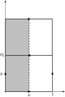
Figure 1.4: Fundamental polygons for the Klein-bottle.

The Klein-bottle projects the states that propagate in the torus to give the propagation of an unoriented closed string at one loop. The modulus of the Klein-bottle is purely imaginary, $\tau=i\tau_{2}$, and the fundamental polygon for it, obtained cutting its surface, is a rectangle with the horizontal side rescaled to one, the vertical side equal to $i\tau_{2}$, and the opposite sides identified after a change of the relative orientation for the horizontal ones (see figure 3.2). A vertical doubling of the fundamental polygon of the Klein-bottle gives the doubly-covering torus with Teichmüller parameter equal to $it_{2}=i2\tau_{2}$. The modulus $\tau_{2}$ is interpreted as the proper time that a closed string needs to sweep the Klein-bottle. But there is another choice for the fundamental polygon, obtained halving the horizontal side and doubling the vertical one, so that the area remains unchanged. The vertical sides of the new polygon are actually two crosscaps and the horizontal ones are identified now with the same orientation. This polygon corresponds to a tube ending at two crosscaps, so that the Klein-bottle can also be interpreted as describing a closed string that propagates between two crosscaps in a proper time represented by the horizontal side of the second polygon.

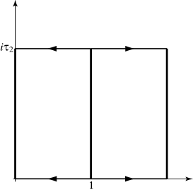
Figure 1.5: Fundamental polygon for the annulus.

The propagation at one loop of an oriented open string is described by the annulus. After a cut it is mapped into a rectangle with the horizontal sides identified (see figure 3.3). The vertical ones are the two boundaries of the annulus. The modulus of the annulus is once more purely imaginary, $\tau=i\tau_{2}$, and represents the proper time elapsed while an open string sweeps it. The doubly-covering torus is obtained doubling the horizontal sides and its Teichmüller parameter is $it_{2}=i\frac{\tau_{2}}{2}$. But there is another equivalent representation of the annulus as a tube that ends in two boundaries. In this new picture, we can see a closed string that propagates between the two boundaries, and the modulus of the tube is just the proper time elapsed in this propagation.

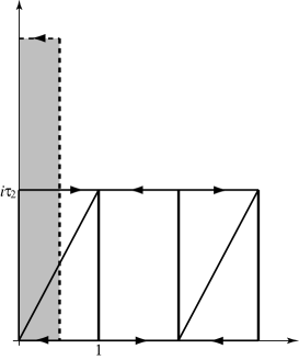
Figure 1.6: Fundamental polygons for the Möbius strip.

Finally, at genus $g=1$ we have also the Möbius strip, that projects the annulus amplitude to describe the one loop propagation of an unoriented open string. The fundamental polygon is a rectangle where the horizontal sides are identified with the opposite orientation (see figure 1.6). The two vertical sides together form the boundary of the Möbius strip. The modulus is $i\tau_{2}$ and has the meaning of the time elapsed while the open string sweeps the Möbius. The doubly covering torus in this case is not obtained simply horizontally or vertically doubling the polygon but horizontally doubling two times it (see figure 1.6). The result is that the Teichmüller parameter of the torus now is not purely imaginary but has a real part: $t=\frac{1}{2}+i\frac{\tau_{2}}{2}$. Also in the case of the Möbius strip it is possible to give an equivalent representation of the surface, halving the horizontal side while doubling the vertical one. The vertical sides are now a boundary and a crosscap and the horizontal side is the proper time elapsed while a closed string propagates from the boundary to the crosscap trough a tube.

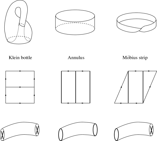
Figure 1.7: Klein-bottle, annulus and Möbius strip.

In the following, we will refer to the amplitudes corresponding to the first fundamental polygon as the amplitudes in the direct channel, while the other choice describes the amplitudes in the transverse channel. The direct and transverse channels are related through an $S$-modular transformation that maps the “vertical time” of the direct channel in to the “horizontal time” of the transverse one. A subtlety for the Möbius strip is due to the fact that the modulus of the doubly covering torus is not purely imaginary and we will come back to this point in the following.

1.3 The torus partition function

After having introduced the Riemann surfaces with vanishing Euler characteristic, corresponding in String Theory to the one-loop vacuum amplitudes, we can begin to write their partition functions. We start at first from the simplest case of field theory, deriving the one loop vacuum energy for a massive scalar field in $D$ dimensions

$$S^{(E)}\ =\ \int\ d^{D}x\ \frac{1}{2}\ \left(\partial_{\mu}\phi\ \partial^{\mu}\phi+M^{2}\phi^{2}\right)\ .$$ (1.37)

The one loop vacuum energy $\Gamma$ is expressed trough the relation

$$e^{-\Gamma}\ =\ \int[\mathcal{D}\phi]\ e^{-S^{(E)}}\sim\left[\mathrm{det}(-\Box+M^{2})\right]^{-\frac{1}{2}}\ ,$$ (1.38)

that means

$$\Gamma\ =\ \frac{1}{2}\mathrm{tr}\left[\ln(-\Box+M^{2})\right]\ .$$ (1.39)

Using the formula for the trace of the logarithm of a matrix $A$

$$\mathrm{tr}(\ln{A})\ =\ -\int_{\epsilon}^{\infty}\frac{dt}{t}\ \mathrm{tr}\left(e^{-tA}\right)\ ,$$ (1.40)

where $\epsilon$ is an ultraviolet cut-off, and inserting a complete set of eigenstates of the kinetic operator, we get:

$$\Gamma\ =\ -\frac{V}{2}\int_{\epsilon}^{\infty}\frac{dt}{t}\ \int\frac{d^{D}p}{(2\pi)^{D}}\ e^{-tp^{2}}\ \mathrm{tr}\left(e^{-tM^{2}}\right)\ ,$$ (1.41)

where $V$ is the space-time volume. The integral on $p$ is gaussian and can be computed. The result is that the one loop vacuum energy for a bosonic degree of freedom is

$$\Gamma\ =\ -\frac{V}{2(4\pi)^{\frac{D}{2}}}\ \int_{\epsilon}^{\infty}\frac{dt}{t^{\frac{D}{2}+1}}\ \mathrm{tr}\left(e^{-tM^{2}}\right)\ .$$ (1.42)

For a Dirac fermion there is only a change of sign due to the anticommuting nature of the integration variables, and we have also to multiply for the number of degrees of freedom of a Dirac fermion that in $D$ dimension is $2^{\frac{D}{2}}$. The end result, for a theory with bosons and fermions is

$$\Gamma\ =\ -\frac{V}{2(4\pi)^{\frac{D}{2}}}\ \int_{\epsilon}^{\infty}\frac{dt}{t^{\frac{D}{2}+1}}\ \mathrm{Str}\left(e^{-tM^{2}}\right)\ ,$$ (1.43)

where the supertrace $\mathrm{Str}\$ is

$$\mathrm{Str}\ =\ \sum_{bosons}\ -\ 2^{\frac{D}{2}}\sum_{fermions}\ .$$ (1.44)

We now use the expression (1.43) in the case of superstring theory, recalling the mass formula (1.31), that here we report in terms of $L_{0}^{\bot}=N_{B}+N_{F}$ and $\bar{L}_{0}^{\bot}=\bar{N}_{B}+\bar{N}_{F}$

$$M^{2}\ =\ \frac{2}{\alpha^{\prime}}\ \left[L_{0}^{\bot}+\bar{L}_{0}^{\bot}+a+\bar{a}\right]\ .$$ (1.45)

In order to take properly into account the level-matching condition for the physical states, we have to introduce a delta-function in the integral (1.43). Setting the dimension to the critical value $D=10$ gives

$$\Gamma\ =\ -\frac{V}{2(4\pi)^{5}}\ \int_{-\frac{1}{2}}^{\frac{1}{2}}ds\int_{\epsilon}^{\infty}\frac{dt}{t^{6}}\ \mathrm{Str}\left(e^{-\frac{2}{\alpha^{\prime}}\left[L_{0}^{\bot}\ +\ \bar{L}_{0}^{\bot}\ +\ a\ +\ \bar{a}\right]t}\ e^{2\pi i\left[L_{0}^{\bot}\ +\ a\ -\ \bar{L}_{0}^{\bot}\ -\ \bar{a}\right]s}\right)\ ,$$ (1.46)

that, defining $\tau=s+i\frac{t}{\pi\alpha^{\prime}}\$ and $q\ =\ e^{2\pi i\tau}\$, $\ \bar{q}\ =\ e^{-2\pi i\bar{\tau}}\$, becomes

$$\Gamma\ =\ -\frac{V}{2(4\alpha^{\prime}\pi^{2})^{5}}\ \int_{-\frac{1}{2}}^{\frac{1}{2}}d\tau_{1}\int_{\epsilon}^{\infty}\frac{d\tau_{2}}{\tau_{2}^{6}}\ \mathrm{Str}\left(q^{\ L_{0}^{\bot}+a}\ \bar{q}^{\ \bar{L}_{0}^{\bot}+\bar{a}}\right)\ .$$ (1.47)

This is the partition function for a closed string that propagates in a loop, so that it is the torus amplitude with $\tau$ its Teichmüller parameter. Recalling that all inequivalent tori correspond to values of $\tau$ in the fundamental region $\mathcal{F}$, and apart from an overall normalization constant, we can write the torus amplitude in the form

$$\mathcal{T}\ =\ \int_{\mathcal{F}}\frac{d^{2}\tau}{\tau_{2}^{2}}\ \frac{1}{\tau_{2}^{4}}\ \mathrm{Str}\left(q^{\ L_{0}^{\bot}+a}\ \bar{q}^{\ \bar{L}_{0}^{\bot}+\bar{a}}\right)\ .$$ (1.48)

Let us remark again that the modular invariance of $\mathcal{T}$ (that we will check in a while) allows one to exclude from the integration region the ultraviolet point $\tau=0$, where the integrand would diverge.

At this point we have to compute the traces. In the NS sector $a=-\frac{1}{2}$ and the trace is

$$\mathrm{tr}\ q^{\ N_{B}+N_{F}-\frac{1}{2}}\ =\ \frac{1}{\sqrt{q}}\ \mathrm{tr}\left(q^{\ \sum_{n=1}^{\infty}\alpha_{-n}^{i}\alpha_{n}^{i}}\right)\ \mathrm{tr}\left(q^{\ \sum_{r=\frac{1}{2}}^{\infty}r\ b_{-r}^{i}b_{r}^{i}}\right)\ ,$$ (1.49)

where a sum over $i=1\ldots 8$ is understood. The bosonic trace is like the partition function for a Bose gas. Using the algebra (1.1.2), a state with $k$ oscillators of frequency $n$ gives a contribution $q^{nk}$, so that we have to compute

$$\prod_{i=1}^{8}\prod_{n=1}^{\infty}\sum_{k}q^{nk}$$ (1.50)

and the result is

$$\frac{1}{\prod_{n=1}(1-q^{n})^{8}}\ .$$ (1.51)

The fermionic trace is instead like the partition function of a Fermi-Dirac gas. By the Pauli exclusion principle, any oscillator can have occupation number only equal to $0$ or $1$, and thus the fermionic trace is simply

$$\prod_{i=1}^{8}\prod_{r=1/2}(1+q^{r})\ .$$ (1.52)

In the R sector $a=0$, and we have to multiply by $2^{\frac{D-2}{2}}=16$ to take into account the degeneracy of the Ramond vacuum. Putting the bosonic and the fermionic contributions together gives

$$\mathrm{tr}\ q^{\ N_{B}+N_{F}-\frac{1}{2}}\ = \ \frac{\prod_{r=1/2}(1+q^{r})^{8}}{\sqrt{q}\ \prod_{n=1}(1-q^{n})^{8}}\quad(NS),$$

$$\mathrm{tr}\ q^{\ N_{B}+N_{F}}\ = \ 16\ \frac{\prod_{n=1}(1+q^{n})^{8}}{\prod_{n=1}(1-q^{n})^{8}}\quad(R)\ .$$ (1.53)

The previous quantities can be expressed in terms of the Jacobi $\vartheta$-functions of argument $z=0$

$$\vartheta\left[{\textstyle{\alpha\atop\beta}}\right](z|\tau)=\sum_{n}\ q^{\frac{1}{2}(n+\alpha)^{2}}\ e^{2\pi i(n+\alpha)(z+\beta)}\ ,$$ (1.54)

where $\ \alpha,\beta=0,\ \frac{1}{2}\$. Equivalently the Jacobi $\vartheta$-functions can be defined by the infinite products

$$\vartheta\left[{\textstyle{\alpha\atop\beta}}\right](z|\tau) = e^{2i\pi\alpha(z+\beta)}\ q^{\alpha^{2}/2}\prod_{n=1}^{\infty}\ (1-q^{n})\prod_{n=1}^{\infty}\ (1+q^{n+\alpha-1/2}e^{2i\pi(z+\beta)})$$ (1.55)

$$\times\prod_{n=1}^{\infty}(1+q^{n-\alpha-1/2}e^{-2i\pi(z+\beta)})\ .$$

Moreover, we have to introduce the Dedekind $\eta$-function

$$\eta(\tau)\ =\ q^{\frac{1}{24}}\prod_{n=1}^{\infty}\ (1-q^{n})\ .$$ (1.56)

Using the definition (1.56) and (1.55), it is then possible to write the following quantities:

$$\frac{\vartheta^{4}\left[{\small 1/2}\atop{\small 1/2}\right](0|\tau)}{\eta^{12}(\tau)}=\frac{\vartheta_{1}^{4}(0|\tau)}{\eta^{12}(\tau)}=0\,,$$ (1.57)

$$\frac{\vartheta^{4}\left[{\small 1/2}\atop{\small 0}\right](0|\tau)}{\eta^{12}(\tau)}=\frac{\vartheta_{2}^{4}(0|\tau)}{\eta^{12}(\tau)}=16\frac{\prod_{n=1}^{\infty}(1+q^{n})^{8}}{\prod_{n=1}^{\infty}(1-q^{n})^{8}}\,,$$ (1.58)

$$\frac{\vartheta^{4}\left[{\small 0}\atop{\small 0}\right](0|\tau)}{\eta^{12}(\tau)}=\frac{\vartheta_{3}^{4}(0|\tau)}{\eta^{12}(\tau)}=\frac{\prod_{n=1}^{\infty}(1+q^{n-1/2})^{8}}{q^{1/2}\prod_{n=1}^{\infty}(1-q^{n})^{8}}\,,$$ (1.59)

$$\frac{\vartheta^{4}\left[{\small 0}\atop{\small 1/2}\right](0|\tau)}{\eta^{12}(\tau)}=\frac{\vartheta_{4}^{4}(0|\tau)}{\eta^{12}(\tau)}=\frac{\prod_{n=1}^{\infty}(1-q^{n-1/2})^{8}}{q^{1/2}\prod_{n=1}^{\infty}(1-q^{n})^{8}}\ ,$$ (1.60)

that are directly related to the ones that appear in the string amplitudes after the GSO projection

$$\mathrm{tr}\ \left[q^{\ N_{B}+N_{F}-\frac{1}{2}}\ \frac{1-(-1)^{F}}{2}\right]\ = \ \frac{1}{\eta^{8}}\ \frac{\vartheta_{3}^{4}(0|\tau)-\vartheta_{4}^{4}(0|\tau)}{2\eta^{4}(\tau)}\quad(NS)$$

$$\mathrm{tr}\ \left[q^{\ N_{B}+N_{F}}\ \frac{1\pm\Gamma_{9}(-1)^{F}}{2}\right]\ = \ \frac{1}{\eta^{8}}\ \frac{\vartheta_{2}^{4}(0|\tau)\pm\vartheta_{1}^{4}(0|\tau)}{2\eta^{4}(\tau)}\quad(R)\ ,$$ (1.61)

where the sign in the Ramond sector selects the chirality of the vacuum. The four $\vartheta$-functions are related to the four spin structures of the fermionic determinant on the torus, and $\vartheta_{1}$ vanishes because it is the contribution of the periodic-periodic structure that is the only one which containing a zero-mode. In order to have a modular invariant partition function, we need all the four GSO-projected sectors NS-NS, NS-R, R-NS, R-R. Let us note again the importance of the projection, that is instrumental to reconstruct the modular invariant.

At this point, it is useful to introduce the characters of the affine extension $(k=1)$ of the algebra $so(8)$, decomposing into two orthogonal subspaces both the NS and the R sectors

$$O_{8}\ = \ \frac{\vartheta_{3}^{4}+\vartheta_{4}^{4}}{2\eta^{4}}\qquad\qquad V_{8}\ =\ \frac{\vartheta_{3}^{4}-\vartheta_{4}^{4}}{2\eta^{4}}\qquad\qquad(NS)$$

$$S_{8}\ = \ \frac{\vartheta_{2}^{4}+\vartheta_{1}^{4}}{2\eta^{4}}\qquad\qquad C_{8}\ =\ \frac{\vartheta_{2}^{4}-\vartheta_{1}^{4}}{2\eta^{4}}\qquad\qquad(R)\ .$$ (1.62)

Each of these characters in the language of CFT is a trace over the corresponding Verma module (or conformal family) that consists in an infinite tower of descendants of increasing mass and spin whose state with the lowest conformal weight $L_{0}^{\bot}=h$ is called the primary field. The general form of a character is

$$\chi(q)\ =\ q^{h-c/24}\sum_{k}d_{k}q^{k},$$ (1.63)

where $c$ is the central charge, that is $c=12$ if we take into account also the bosonic degrees of freedom dividing the characters of $so(8)$ by $\eta^{8}$, $h$ is the conformal weight of the primary field, $h+k$ are the conformal weights of the descendants and the $d_{k}$ are integers. For example $O_{8}/\eta^{8}$ starts with a scalar tachyon of conformal weight $\ h=0\$ and squared mass proportional to $-\frac{1}{2}$. $\ V_{8}/\eta^{8},\ S_{8}/\eta^{8},\$ and $\ C_{8}/\eta^{8}\$ start respectively with a massless vector, a massless left Majorana-Weyl spinor and a massless right Majorana-Weyl spinor, that have the same conformal weight $\ h=\frac{1}{2}\$.

The partition function for the torus can now be written rather simply. Then, if the relative chirality of the left and right R sectors is the same, we get the torus partition function for the Type IIB string,

$$\mathcal{T}_{IIB}\ =\ \int\frac{d^{2}\tau}{\tau_{2}^{2}}\ \frac{1}{\tau_{2}^{4}\ (\eta\ \bar{\eta})^{8}}\ |V_{8}-S_{8}|^{2}\ ,$$ (1.64)

otherwise we get the partition function for the Type IIA string,

$$\mathcal{T}_{IIA}\ =\ \int\frac{d^{2}\tau}{\tau_{2}^{2}}\ \frac{1}{\tau_{2}^{4}\ (\eta\ \bar{\eta})^{8}}\ (\bar{V}_{8}-\bar{S}_{8})\ (V_{8}-C_{8})\ .$$ (1.65)

Let us note the minus sign in front of $S_{8}$ and $C_{8}$, due to their fermionic nature. The factor $1/(\eta\bar{\eta})^{8}$ is the contribution of the $8$ world-sheet bosonic degrees of freedom.

We can write rather simply also the torus partition function for the bosonic string, where we do not have any fermionic oscillators and there are $D-2=24$ bosonic degrees of freedom, each of which contributes a factor $1/\sqrt{\tau_{2}}\ |\eta(\tau)|^{2}$, giving a torus amplitude equal to

$$\mathcal{T}_{\it bosonic}\ =\ \int\frac{d^{2}\tau}{\tau_{2}^{2}}\ \frac{1}{\tau_{2}^{12}\ (\eta\ \bar{\eta})^{24}}\ .$$ (1.66)

Coming back to the superstring, and after what we said about the characters, it is simple to read off the low-energy spectra of the Type IIA and IIB theories from their partition functions and to convince oneself that they coincide with the ones we already recovered at the end of the first section. For example, $V_{8}\bar{V}_{8}$ contains the graviton, the dilaton and the antisymmetric 2-tensor, both in the type IIA and type IIB supergravity. Moreover, the type IIB superstring contains another scalar another 2-form and a 4-form with self-dual field-strength that come from $S_{8}\bar{S}_{8}$, two gravitinos with the same chirality and two dilatinos also with the same chirality that come from $V_{8}\bar{S}_{8}+S_{8}\bar{V}_{8}$. For the type IIA supergravity $S_{8}\bar{C}_{8}$ gives an abelian vector and a 3-form, while the mixed term gives two gravitinos and two dilatinos with opposite chiralities.

An important thing to observe is that the relation

$$\vartheta_{3}^{4}-\vartheta_{4}^{4}-\vartheta_{2}^{4}\ =\ 0\ ,$$ (1.67)

known as the aequatio identica satis abstrusa of Jacobi, implies $\ V_{8}-S_{8}=0\$, which means that at each level the spectrum of Type IIB superstring contains the same number of fermionic and bosonic degrees of freedom, and again this happens thanks to the GSO-projection.

We can now discuss the modular invariance of the amplitudes we wrote. First of all, the integration measure is invariant. The transformation laws for the Dedekind function

$$T\ :\ \eta(\tau)\rightarrow\eta(\tau+1)\ =\ e^{\frac{i\pi}{12}}\ \eta(\tau)\ ,\qquad S\ :\ \eta(\tau)\rightarrow\eta\left(-\frac{1}{\tau}\right)\ =\ \sqrt{-i\tau}\ \eta(\tau)\ ,$$ (1.68)

then imply that also the denominator $\tau_{2}^{4}\ (\eta\bar{\eta})^{8}$ is clearly invariant. The modular invariance of the torus is then demonstrated if we consider that on the basis $\ O_{8}\ ,\ V_{8}\ ,\ S_{8}\ ,\ C_{8}\$ a $T$-modular transformation acts like

$$T=e^{-i\pi/3}\ {\rm diag}\left(1,-1,-1,-1\right)\ ,$$ (1.69)

that can be proved recalling that the form of the characters is of the type given in (1.63) with $c=4$ (because the $so(8)$ characters contain only the contribution of the fermionic oscillators), while an $S$-modular transformation is described by

$$S=\frac{1}{2}\ \left(\begin{array}[]{rrrr}1&1&1&1\\ 1&1&-1&-1\\ 1&-1&1&-1\\ 1&-1&-1&1\end{array}\right)\ ,$$ (1.74)

that can be determined from the $S$-modular transformation law for $\vartheta$-functions

$$\vartheta\left[{\textstyle{\alpha\atop\beta}}\right]\left(\frac{z}{\tau}\right|\left.-\frac{1}{\tau}\right)=(-i\tau)^{1/2}\ e^{2i\pi\alpha\beta+i\pi z^{2}/\tau}\ \vartheta\left[{\textstyle{\beta\atop-\alpha}}\right](z|\tau)\ .$$ (1.75)

For completeness, here we give also the $T$-modular transformation

$$\vartheta\left[{\textstyle{\alpha\atop\beta}}\right](z|\tau+1)=e^{-i\pi\alpha(\alpha-1)}\vartheta\left[{\textstyle{\alpha\atop\beta+\alpha-1/2}}\right](z|\tau)\ .$$ (1.76)

Before closing this part, we would like to reconsider the torus partition function from the point of view of CFT [34, 35]. In fact, apart from the integral with its measure, the general form of a torus partition function is

$${\cal T}\ =\ \sum_{i,j}\bar{\chi}_{i}X_{ij}\chi_{j}\ ,$$ (1.77)

where $X_{ij}$ is a matrix of non negative integer numbers, that for the rational models is finite-dimensional. Modular invariance restricts the general form of $X_{ij}$, imposing the constraints

$$S^{\dagger}\,X\,S=X\,,\qquad T^{\dagger}\,X\,T=X\ .$$ (1.78)

This observation is very important and will allow us to write in the next chapter the torus partition functions for the type 0 models.

1.4 The orientifold projection

This section is devoted to review the orientifold projection for the Superstring Theory [13, 65, 45, 69, 66, 60, 46, 47]. This is an algorithm to build a consistent theory of unoriented closed and open strings. The starting point is a torus partition function for the Type IIB string that is left-right symmetric. The resulting model is known as the Type I string. In order to make the string unoriented, we have to identify the left and right modes of the string, projecting the spectrum to left-right symmetric or antisymmetric states. The projection has to be consistent with the interacting theory, and this means that only one of the two possible choices can be implemented. Actually, what we have to do is insert in the trace of (1.48) the projector $P=\frac{1+\Omega}{2}$, where $\Omega$ is the world-sheet parity, whose action is to exchange the left $(L)$ oscillators with the right $(R)$ ones. The result is that $\mathcal{T}\rightarrow\mathcal{T}/2+\mathcal{K}$, where $\mathcal{K}$ is the partition function for the Klein-bottle

$${\cal K}\ =\ \frac{1}{2}\int_{0}^{\infty}\ \frac{d^{2}\tau}{\tau_{2}^{6}}\ \mathrm{Str}\ \left(q^{L_{0}^{\bot}-a}\bar{q}^{\bar{L}_{0}^{\bot}-\bar{a}}\Omega\right)\ .$$ (1.79)

The trace to perform is

$$\sum_{L,R}\langle L,R\mid q^{L_{0}^{\bot}-a}\bar{q}^{\bar{L}_{0}^{\bot}-\bar{a}}\Omega\mid L,R\rangle\ =\ \sum_{L,R}\langle L,R\mid q^{L_{0}^{\bot}-a}\bar{q}^{\bar{L}_{0}^{\bot}-\bar{a}}\mid R,L\rangle\ ,$$ (1.80)

and using the orthogonality of the states, we can reduce this to the sum over only the diagonal sub-space, identifying effectively $L_{0}^{\bot}$ with $\bar{L}_{0}^{\bot}$,

$$\sum_{L}\langle L\mid(q\bar{q})^{L_{0}^{\bot}-a}\mid L\rangle\ .$$ (1.81)

The last expression depends naturally from $2i\tau_{2}$, which we recognize as the modulus of the doubly covering torus for the Klein-bottle. Moreover, we understand that the mixed sectors in the torus have to be simply halved because their contribution after the action of $\Omega$ would be zero for orthogonality. Performing the last sum, we get

$${\cal K}=\frac{1}{2}\int_{0}^{\infty}\ \frac{d\tau_{2}}{\tau_{2}^{6}}\ \frac{(V_{8}-S_{8})(2i\tau_{2})}{\eta^{8}(2i\tau_{2})}\ .$$ (1.82)

The projection symmetrizes the NS-NS sector and antisymmetrizes the R-R sector, while the mixed sectors in $\mathcal{T}$ are simply halved, as we said. This is consistent with the fusion rules between the conformal families corresponding to the characters $V_{8},\ O_{8},\ -S_{8},\ -C_{8}$. These rules, encoded in the Verlinde formula [48], say that $V_{8}$ behaves like the identity in the fusion with the other characters, while $-S_{8}$ fuses with $-C_{8}$ to give $O_{8}$.

The resulting massless spectrum is obtained from the Type IIB one eliminating the $2$-form from the NS-NS sector, the scalar and the $4$-form from the R-R sector, one gravitino and one dilatino from the mixed sector. What survives the projection is a graviton, a dilaton and a RR $2$-form for the bosons, and a gravitino and a dilatino of opposite chirality for the fermions. This spectrum corresponds to the $\mathcal{N}=1$ minimal supergravity in $D=10$ dimensions.

In order to go in the transverse channel, the first thing to do is to express (1.82) in terms of the modulus of the doubly covering torus, and the change of variable $2\tau_{2}=t_{2}$, (1.82) uncovers the important factor $2^{5}$. Then we have to perform an $S$ modular transformation: $t_{2}\rightarrow 1/\ell$, where $\ell$ is the time in the transverse channel. The “supercharacter” $(V_{8}-S_{8})$ is invariant, while the factor $t_{2}^{4}\eta(it_{2})^{8}\rightarrow\eta(i\ell)^{8}$, and thus the transverse Klein-bottle is

$$\tilde{\cal K}=\frac{2^{5}}{2}\int_{0}^{\infty}\ d\ell\ \frac{(V_{8}-S_{8})(i\ell)}{\eta^{8}(i\ell)}\,.$$ (1.83)

Let us stress that (1.83) is a sum over the characters $V_{8}$ and $-S_{8}$ flowing in the transverse channel, each of which is multiplied by a positive coefficient that can be interpreted as the square of the one-point function of the character in front of the crosscap. The Klein-bottle projection has must be consistent with the positivity of these coefficients in the transverse channel, as in fact is the case in (1.83).

At this point we introduce the open strings. As we already saw in the first section, an open string allows the propagation of the vector and therefore it describes naturally the Yang-Mills interaction. The important thing to stress is that a scattering amplitude with only open strings is planar and, as was observed by Chan and Paton [49], its cyclic symmetry remains preserved also multiplying the amplitude for a factor that is the trace over the product of matrices of a certain gauge group. So, it is possible to associate to an open string a Chan-Paton matrix or equivalently to attach at the ends of the string some Chan-Paton charges. Marcus and Sagnotti showed that the Chan-Paton group can be only one of the classical groups [50], thus excluding the exceptional groups.

Let us begin to write the one-loop partition function for an oriented open string. Its general form is

$$N^{2}\ \int_{0}^{\infty}\ \frac{d\tau_{2}}{\tau_{2}^{6}}\ {\rm Str}\ q^{\frac{1}{2}(L_{0}^{\bot}-a)}\ ,$$ (1.84)

where $N$ is the multiplicity of the Chan-Paton charges. Let us note the factor $\frac{1}{2}$ in the exponent, reflecting the different mass-shell condition for an open string. This factor will make the annulus depend on the modulus of the doubly covering torus.

The amplitudes for unoriented open strings are obtained inserting in the trace the projector $P=(1+\epsilon\Omega)/2$, where the world-sheet parity $\Omega$ flips the ends of the string, $\Omega:\sigma\rightarrow\pi-\sigma$, while $\epsilon$ is a sign that will be fixed in order to have a consistent model. After the projection, the trace (1.84) splits in the amplitude for the annulus

$${\cal A}=\frac{N^{2}}{2}\int_{0}^{\infty}\ \frac{d\tau_{2}}{\tau_{2}^{6}}\ \frac{(V_{8}-S_{8})(\frac{1}{2}i\tau_{2})}{\eta^{8}({\textstyle{1\over 2}}i\tau_{2})}\ ,$$ (1.85)

and the amplitude for the Möbius strip

$${\cal M}=\frac{\epsilon N}{2}\int_{0}^{\infty}\ \frac{d\tau_{2}}{\tau_{2}^{6}}\ \frac{(\hat{V}_{8}-\hat{S}_{8})({\textstyle{1\over 2}}i\tau_{2}+{\textstyle{1\over 2}})}{\hat{\eta}^{8}({\textstyle{1\over 2}}i\tau_{2}+{\textstyle{1\over 2}})}\ .$$ (1.86)

The last amplitude is understood if we consider that $\Omega$ acts on a state $\alpha_{-n}\mid ij\rangle$ (where $i,j$ run on the multiplicity of the Chan-Paton charges at the end of the string) giving $(-)^{n}\alpha_{-n}\mid ji\rangle$. Thus, when we compute the trace, the sum over $i,j$ is restricted only to the diagonal states $\mid i\rangle$, giving a factor $N$, while $q^{\frac{n}{2}}$ is shifted to $q^{\frac{n}{2}}(-)^{n}$, that means $e^{2\pi in(1/2+i\tau_{2}/2)}$, in which we recognize the modulus of the doubly covering torus. In order to have a real integrand for the Möbius strip, we introduced the real hatted characters whose generic form is

$$\hat{\chi}(i\tau_{2}+{\textstyle{1\over 2}})=q^{h-c/24}\sum_{k}(-1)^{k}d_{k}q^{k}\ ,\qquad q=e^{-2\pi\tau_{2}}\ ,$$ (1.87)

that differ from the standard $\chi(i\tau_{2}+1/2)$ in the overall phase $e^{-i\pi(h-c/24)}$.

The transverse channel for the Annulus amplitude is simply obtained making the change of variable $\frac{\tau_{2}}{2}=t_{2}$, that gives an overall factor $2^{-5}$, and then performing an $S$ transformation $t_{2}\rightarrow\frac{1}{\ell}$:

$$\tilde{\cal A}=\frac{2^{-5}\ N^{2}}{2}\int_{0}^{\infty}\ d\ell\ \frac{(V_{8}-S_{8})(i\ell)}{\eta^{8}(i\ell)}\ .$$ (1.88)

Note that also for the transverse annulus the characters $V_{8}$ and $-S_{8}$ are multiplied by positive numbers whose square roots are the one-point functions of those characters in front of the boundaries.

Writing the transverse channel for the Möbius presents some subtleties due to the real part of $\tau$, and as a result, the transformation $\tau_{2}\rightarrow 1/t$ is achieved performing a $P=T^{1/2}ST^{2}ST^{1/2}$ transformation [51]. On the basis

$$\frac{O_{8}}{\tau_{2}^{4}\eta^{8}}\,,\quad\frac{V_{8}}{\tau_{2}^{4}\eta^{8}}\,,\quad\frac{S_{8}}{\tau_{2}^{4}\eta^{8}}\,,\quad\frac{C_{8}}{\tau_{2}^{4}\eta^{8}}$$ (1.89)

the action of $T$ is simply $T=\ {\rm diag}(-1,1,1,1)\$, so that, considering that $S$ squares to the conjugation matrix, that is the identity for $so(8)$ because its representations are self-conjugate, the $P$ matrix takes the very simple form

$$P\ =\ T\ ={\rm diag}(-1,1,1,1)\ ,$$ (1.90)

apart from an overall power of $\tau_{2}$ that disappears in the transverse channel. In terms of $\ell=t/2$ the transverse Möbius amplitude then reads

$$\tilde{\cal M}=2\ \frac{\epsilon N}{2}\int_{0}^{\infty}\ d\ell\ \frac{(\hat{V}_{8}-\hat{S}_{8})(i\ell+{\textstyle{1\over 2}})}{\hat{\eta}^{8}(i\ell+{\textstyle{1\over 2}})}\ .$$ (1.91)

Naïvely the transverse Möbius amplitude, that is a tube between a crosscap and a boundary, can be seen as the geometric mean $\sqrt{\tilde{\cal K}\tilde{\cal A}}$, so that the factor $2$ in (1.91) is a combinatoric factor, while the sign $\epsilon$ reflects the sign ambiguity of the one-point functions in front of the crosscap and of the boundary, that we know only squared from $\tilde{\cal A}$ and $\tilde{\cal K}$.

The massless spectrum, that we read from the direct channel, gives the $N=1$ super Yang-Mills multiplet in $D=10$ and consists of a vector and a Majorana-Weyl fermion with multiplicity $N(N-\epsilon)/2$. Therefore, $\epsilon=1$ corresponds to the adjoint representation of the gauge group $SO(N)$, while $\epsilon=-1$ corresponds to the adjoint representation of $USp(N)$.

At this point it is useful to summarize the orientifold construction. To this end, let us consider the general form of the torus partition function (1.77)

$${\cal T}\ =\ \sum_{i,j}\bar{\chi}_{i}X_{ij}\chi_{j}\ ,$$ (1.92)

with its constraints (1.78). Moreover let us suppose that $X_{ij}=0,1$. A value of $X_{ij}$ different from $0,1$ means that we have more conformal families starting with the same conformal weight, and thus we have to resolve an ambiguity.

In the Klein-bottle only the left-right symmetric sectors can propagate, the ones with $X_{ii}\neq 0$

$${\cal K}\ =\ \frac{1}{2}\sum_{i}{\cal K}^{i}\chi_{i}\ ,\qquad\qquad{\cal K}^{i}=\pm X_{ii}\ .$$ (1.93)

While in the transverse channel we read

$$\tilde{\cal K}=\frac{1}{2}\sum_{i}({\Gamma}^{i})^{2}\,\chi_{i}\ .$$ (1.94)

The coefficients $\Gamma_{i}$ are the one-point functions (or the reflection coefficients) of $\chi_{i}$ in front of a crosscap. The signs of ${\cal K}^{i}$ have to be chosen in order to have a consistent interacting theory with positive coefficients $(\Gamma^{i})^{2}$ in the transverse channel.

The transverse annulus has the form

$$\tilde{\cal A}=\frac{1}{2}\sum_{i}\,\chi_{i}\left(\sum_{a}B^{i}_{a}\,n^{a}\right)^{2}\ ,$$ (1.95)

where $B_{a}^{i}$ is the one-point function of $\chi_{i}$ in front of a hole with boundary condition labelled by the index $a$ and where $n^{a}$ is the corresponding Chan-Paton multiplicity. As a bulk sector reflecting on a boundary turns into its conjugate, the transverse annulus propagates only the characters $\chi_{i}$ that appear in the torus in the form $\bar{\chi}_{i}^{C}\chi_{i}$, where $\chi_{i}^{C}$ is the conjugate of $\chi_{i}$. In the case of $X=\mathcal{C}$, where $\mathcal{C}$ is the conjugation matrix, all bulk sectors can reflect on a hole and the number of different boundary conditions is equal to the number of bulk sectors. One can turn an important observation of Cardy [52] on the annulus amplitude into an ansatz to write the orientifold of a theory with $X=\mathcal{C}$. But let us to proceed with the general case. After an $S$-modular transformation we get the direct channel for the annulus

$${\cal A}=\frac{1}{2}\sum_{i,a,b}\,{\cal A}^{i}_{ab}\,n^{a}\,n^{b}\,\chi_{i}\,.$$ (1.96)

Finally, the transverse Möbius, apart from a combinatoric factor $2$, is the square root of $\tilde{\cal K}\times\tilde{\cal A}$

$$\tilde{\cal M}=\frac{1}{2}\sum_{i}\,\hat{\chi}_{i}\,{\Gamma}^{i}\left(\sum_{a}B^{i}_{a}\,n^{a}\right)\ ,$$ (1.97)

while in the direct channel it reads

$${\cal M}={\textstyle\frac{1}{2}}\sum_{i,a}\,{\cal M}^{i}{}_{a}\,n^{a}\,\hat{\chi}_{i}\ .$$ (1.98)

The construction then is consistent if ${\cal M}$ is the projection of ${\cal A}$, meaning that $M^{i}_{a}=\pm A^{i}_{aa}$, supposing $A_{aa}^{i}=0,1\$.

For completeness, now we report also the amplitudes for the bosonic string. The orientifold projection proceeds along the same steps we traced for the superstring, but it is much easier because there are only bosonic oscillators. Apart from the torus partition function, the other amplitudes are [55, 56]

$${\cal K} = \frac{1}{2}\ \frac{1}{\tau_{2}^{12}\ \eta(2i\tau_{2})^{24}}\ ,$$

$${\cal A} = \frac{N^{2}}{2}\ \frac{1}{\tau_{2}^{12}\ \eta({\textstyle{1\over 2}}i\tau_{2})^{24}}\ ,$$

$${\cal M} = \frac{\epsilon\,N}{2}\ \frac{1}{\tau_{2}^{12}\ \hat{\eta}(\frac{1}{2}i\tau_{2}+\frac{1}{2})^{24}}\,,$$ (1.99)

while in the transverse channel they read

$$\tilde{\cal K} = \frac{2^{13}}{2}\ \frac{1}{\eta(i\ell)^{24}}\,,$$

$$\tilde{\cal A} = \frac{2^{-13}\ N^{2}}{2}\ \frac{1}{\eta(i\ell)^{24}}\,,$$

$$\tilde{\cal M} = 2\ \frac{\epsilon\,N}{2}\ \frac{1}{\hat{\eta}(i\ell+{\textstyle{1\over 2}})^{24}}\,,$$ (1.100)

where the integration is understood. The Klein-bottle amplitude symmetrizes the torus, and the resulting unoriented closed spectrum at the massless level contains only the graviton and the dilaton, while the massless unoriented open spectrum has a vector in the adjoint representation of $SO(N)$ or $USp(N)$, depending on the choice of the sign $\epsilon$.

All those amplitudes have an ultraviolet divergence for $\tau_{2}\rightarrow 0$. The origin of this divergence is well understood if we pass in the transverse channel and we consider that a closed string state of squared mass equal to $M^{2}$ and with degeneracy $c_{M}$ enters in those amplitudes with a term proportional to

$$\sum_{M}c_{M}\int_{0}^{\infty}d\ell e^{-\ell M^{2}}\ =\ \sum_{M}c_{M}\left.\frac{1}{p^{2}+M^{2}}\right|_{p^{2}=0}\ .$$ (1.101)

Thus, in the infrared limit $\ell\rightarrow\infty$, the only states that survive are the massless ones, and the propagation of such states at vanishing momentum gives the infrared divergence we said.

Figure 1.8: Tadpole condition.

Nevertheless, it is possible to cancel this divergence noting that in the limit $\ell\rightarrow\infty$ the transverse amplitudes factorize in a one-point function of a massless closed string state in front of a boundary or a crosscap times the propagator of such a state at vanishing momentum times another one-point function. Therefore, eliminating the pole one is imposing the vanishing of the residue. As these one-point functions, that are commonly called tadpoles, depend on $N$ and $\epsilon$, the conditions one imposes, known as tadpole conditions, will fix also the gauge group. For the bosonic string, all the (transverse) infrared divergences cancel by imposing the tadpole condition

$$2^{13}+2^{-13}\ N^{2}-2\,\epsilon\,N=2^{-13}\ (N-\epsilon\,2^{13})^{2}\,,$$ (1.102)

that fixes $\epsilon=+1$ and the gauge group $SO(8192)$ [53, 54, 55, 56].

For the Type I superstring [57], thanks to the supersymmetry, the tadpole condition is the same for both the NS-NS and the R-R sectors

$$\frac{2^{5}}{2}+\frac{2^{-5}\ N^{2}}{2}+2\ \frac{\epsilon N}{2}=\frac{2^{-5}}{2}\ (N+32\epsilon)^{2}=0\ ,$$ (1.103)

and fixes $N=32$ and $\epsilon=-1$. Therefore the gauge group is $SO(32)$.

Let us note that the tadpole cancellation is possible in general only if the model contains both unoriented closed and open strings and that it does not depend on the torus partition function that is free of divergencies due to the modular invariance. The Type I model is free of anomaly thanks to the Green Schwarz mechanism [14].

Although the R-R and NS-NS tadpoles are cancelled at the same time for the Type I superstring, conceptually the tadpole condition in the two sectors has very different meanings. To explain this point, we have to introduce new space-time objects, the D$p$-branes and the O$p$ planes. A D$p$-brane is a dynamical extended object with $p+1$ dimensions. The ends of an open string can attach to it with Dirichlet boundary conditions in the $9-p$ directions orthogonal to the brane and Neumann boundary conditions in the $p+1$ directions parallel to it. These hyperplanes have a tension that is always positive and are charged with respect to a potential described by a $(p+1)$-form [9]. Moreover, there are also $\overline{{\rm D}p}$-branes that have the same tension but the opposite charge. By convention we consider positive the charge of a D$p$-brane and negative the one of a $\overline{{\rm D}p}$-brane.

The O$p$ planes, or orientifold planes, are the fixed points of the world sheet parity, invade $p+1$ dimensions and have no dynamics. They carry a charge with respect to a $(p+1)$-potential and a tension that now can be both positive and negative. Thus there are two types of these hyperplanes together with their conjugates (that have an opposite charge): the O₊ planes with negative tension and charge, the O_- planes with positive tension and charge, the $\overline{\rm O}_{+}$ planes with negative tension and positive charge and the $\overline{\rm O}_{-}$ with positive tension and negative charge.

Actually, the space-time D$p$-branes correspond to the world-sheet boundaries, while the orientifold planes are the space-time counterparts of the crosscaps.

At this point, it should be clear that from the NS-NS and the R-R sectors of the transverse annulus one can read the squared tension of a brane (the tension is the charge for the gravitational field that flows in the NS-NS sector) and its charge (the potentials with respect to the branes are charged are described by the forms flowing in the R-R sector), while from the NS-NS and R-R sectors of the transverse Klein-bottle one can read the tension and the charge of an O-plane.

For example, the Type I superstring contains $N=32$ D$9$-branes and a O$9_{+}$ plane. Coming back to the tadpole condition, now we understood that the R-R tadpole cancellation is related to the charge neutrality of the space-time, and its absence would give quantum anomalies. On the other hand, the NS-NS tadpole condition can be relaxed breaking supersymmetry and giving a dilaton dependent correction to the low-energy effective field theory proportional to

$$\int d^{10}x\sqrt{-g}e^{-\varphi}\ ,$$ (1.104)

where the coefficient in front of the dilaton $\varphi$ is related to the Euler characteristic of the disk.

A term like (1.104) is a source for the gravitational field equation, and hence curves the space-time. The maximally symmetric Minkowski space is no more a solution, and this reflects itself in the infrared divergences that we met in the transverse channel. This crucial point is the heart of this Thesis, and we will deal with it in the last two chapters, where we will show in a number of field theory toy models how to recover the proper finite results starting from a “wrong” vacuum, after suitable resummations are carried up, and where some examples of string models where tadpoles seem not to affect the results, at least at the lowest order, are discussed.

Before closing this section, we would like to describe a first example of a model with a NS-NS tadpole. Starting from the transverse amplitudes $\tilde{\cal A}$ and $\tilde{\cal M}$ of the Type I $SO(32)$ superstring, one can actually generalize them, allowing different signs for the NS-NS and R-R sectors

$$\tilde{\cal A} = \frac{2^{-5}}{2}\int d\ell\ \frac{(n_{+}+n_{-})^{2}\,V_{8}-(n_{+}-n_{-})^{2}\,S_{8}}{\eta^{8}}\,,$$ (1.105)

$$\tilde{\cal M} = \frac{2}{2}\int d\ell\ \frac{\epsilon_{NS}\,(n_{+}+n_{-})\,\hat{V}_{8}-\epsilon_{R}\,(n_{+}-n_{-})\,\hat{S}_{8}}{\hat{\eta}^{8}}\,.$$ (1.106)

From $\tilde{\cal A}$ we see that $n_{+}$ counts the number of D-branes while $n_{-}$ counts the number of $\overline{\rm{D}}$-branes, while the type of O-planes involved depends on the choice of the two signs $\epsilon_{R}$ and $\epsilon_{NS}$. The tadpole conditions in the NS sector

$$\frac{2^{5}}{2}+\frac{2^{-5}\ (n_{+}+n_{-})^{2}}{2}+2\ \frac{\epsilon_{NS}(n_{+}+n_{-})}{2}=0\qquad NS\ ,$$ (1.107)

and in the R sector

$$\frac{2^{5}}{2}+\frac{2^{-5}\ (n_{+}-n_{-})^{2}}{2}+2\ \frac{\epsilon_{R}(n_{+}-n_{-})}{2}=0\qquad R\ ,$$ (1.108)

are clearly solved by the $SO(32)$ superstring, but one can relax the condition in the NS-NS sector. In that case, the R tadpole condition fixes $n_{+}-n_{-}=32$ and $\epsilon_{R}=-1$. The sign $\epsilon_{NS}$ remains still undetermined, and its value specifies the kind of orientifold planes present in the model. In particular, $\epsilon_{NS}=+1$ means that $\overline{\rm O}_{-}$ planes are present, while $\epsilon_{NS}=-1$ means that O₊ planes are present. Let us stress that the simultaneous presence of branes and antibranes brings about a tachyonic instability that reflect their mutual attraction (see, in the direct channel, the tachyonic term $n_{+}n_{-}O_{8}\$)

$${\cal A}\ = \ \frac{1}{2}\int_{0}^{\infty}\,\frac{dt}{t^{6}\eta^{8}}\left[(n_{+}^{2}+n_{-}^{2})\,(V_{8}-S_{8})+2n_{+}n_{-}\,(O_{8}-C_{8})\right]\,,$$ (1.109)

$${\cal M}\ = \ \frac{1}{2}\int_{0}^{\infty}\,\frac{dt}{t^{6}\hat{\eta}^{8}}\left[\epsilon_{NS}\,(n_{+}+n_{-})\,\hat{V}_{8}-\epsilon_{R}\,(n_{+}-n_{-})\,\hat{S}_{8}\right]\ .$$ (1.110)

The spectrum is no more supersymmetric, and a “minimal” choice is the Sugimoto model [58], that corresponds to $n_{+}=0\$, $n_{-}=32$ and $\epsilon_{R}=\epsilon_{NS}=+1$. The resulting spectrum is not supersymmetric, with a massless vector and a massless Majorana-Weyl spinor respectively in the adjoint and in the antisymmetric representation of the gauge group $USp(32)$, but the tachyon instability is no more present.

1.5 Toroidal compactification

In this section we study the compactification of one dimension, say $X$, on a circle $S^{1}$. Certainly the momentum in the compactified dimension is quantized in inverse units of the compactification radius $R\$: $p=m/R\$, but a closed string has also the possibility to wrap itself around the circle $n$ times. The integer $n$ is called the winding number. What we have to do is to identify

$$X(\tau,\sigma)\sim X(\tau,\sigma+\pi)+2\pi Rn\ ,$$ (1.111)

obtaining in this way the expansion

$$X\ =\ x\ +\ 2\alpha^{\prime}\frac{m}{R}\tau+2nR\sigma+i\frac{\sqrt{2\alpha^{\prime}}}{2}\ \sum_{n\neq 0}\left(\frac{\alpha_{n}}{n}\ e^{-2in(\tau-\sigma)}+\frac{\tilde{\alpha}_{n}}{n}\ e^{-2in(\tau+\sigma)}\right)\ .$$ (1.112)

Then, in order to separate also the zero mode in a left and in a right part, it is convenient to introduce

$$p_{L}=\frac{m}{R}+\frac{nR}{\alpha^{\prime}}\ ,\qquad\qquad p_{R}=\frac{m}{R}-\frac{nR}{\alpha^{\prime}}\ .$$ (1.113)

In terms of these momenta $X$ decomposes in $X_{L}+X_{R}$, with

$$X_{L,R}\ =\ \frac{1}{2}x+\alpha^{\prime}p_{L,R}(\tau\mp\sigma)+oscillators\ ,$$ (1.114)

and the mass shell condition becomes

$$m^{2}\ =\ \frac{2}{\alpha^{\prime}}\left[\frac{\alpha^{\prime}}{4}p_{L}^{2}+\frac{\alpha^{\prime}}{4}p_{R}^{2}+L_{0}^{\bot}+\bar{L}_{0}^{\bot}+a+\bar{a}\right]\ ,$$ (1.115)

together with the level-matching condition

$$\frac{\alpha^{\prime}}{4}p_{R}^{2}+L_{0}^{\bot}+a\ =\ \frac{\alpha^{\prime}}{4}p_{L}^{2}+\bar{L}_{0}^{\bot}+\bar{a}\ .$$ (1.116)

In computing the vacuum amplitudes, one has to replace

$$\mathrm{tr}(q^{L_{0}^{\bot}+a}\ \bar{q}^{\bar{L}_{0}^{\bot}+\bar{a}})\ \rightarrow\ \mathrm{tr}\left(q^{L_{0}^{\bot}+a+\frac{\alpha^{\prime}}{4}p_{R}^{2}}\ \bar{q}^{\bar{L}_{0}^{\bot}+\bar{a}+\frac{\alpha^{\prime}}{4}p_{L}^{2}}\right)\ ,$$ (1.117)

and since in equation (1.41) the gaussian integral actually is over the $D-1$ non-compact momenta, a different power of the modulus $\tau_{2}$

$$\frac{1}{\tau_{2}^{D/2+1}}\ \rightarrow\ \frac{1}{\tau_{2}^{(D-1)/2+1}}\$$ (1.118)

is obtained. Therefore, in order to take into account the compactification, what one has to do is to replace in the vacuum amplitudes

$$\frac{1}{\eta\bar{\eta}\ \sqrt{\tau_{2}}}\ \rightarrow\ \sum_{m,n}\frac{q^{\frac{\alpha^{\prime}}{4}p_{R}^{2}}\ \bar{q}^{\frac{\alpha^{\prime}}{4}p_{L}^{2}}}{\eta\bar{\eta}}$$ (1.119)

for each compact dimension.

The quantity on the right-hand side of the previous equation is clearly invariant under a $T$-modular transformation. Proving its invariance under an $S$-modular transformation requires the use of the Poisson transformation

$$\sum_{\{n_{i}\}\in\mathbb{Z}}\,e^{-\pi\,n^{\rm T}\,A\,n\ +\ 2\,i\,\pi\,b^{\rm T}\,n}\ =\ \frac{1}{\sqrt{{\rm det}(A)}}\,\sum_{\{m_{i}\}\in\mathbb{Z}}\,e^{-\pi\,(m-b)^{\rm T}\,A^{-1}\,(m-b)}\,,$$ (1.120)

where, denoting with $d$ the number of compact dimensions, $A$ is a $d\times d$ square matrix and $m$ and $n$ are $d$-dimensional vectors of integers.

For example, the sum in the case of one compact direction, after an $S$ transformation, is in terms of $m$ and $n$

$$\sum_{m,n}e^{-\pi m^{2}\left(\frac{|\tau|^{2}R^{2}}{\alpha^{\prime}\tau_{2}}\right)^{-1}}\ e^{2\pi im\left(\frac{n\tau_{1}}{|\tau|^{2}}\right)}\ e^{\frac{-\pi\tau_{2}n^{2}R^{2}}{\alpha^{\prime}|\tau|^{2}}}\ ,$$ (1.121)

from which we recognize $A^{-1}=|\tau|^{2}R^{2}/\alpha^{\prime}\tau_{2}$ and $b=n\tau_{1}/|\tau|^{2}$. Performing a Poisson resummation with respect to $m$ gives

$$\frac{|\tau|R}{\sqrt{\alpha^{\prime}\tau_{2}}}\sum_{m^{\prime},n}e^{-\frac{\pi|\tau|^{2}R^{2}}{\alpha^{\prime}\tau_{2}}\left(m^{\prime}-\frac{n\tau_{1}}{|\tau|^{2}}\right)^{2}}e^{\frac{-\pi\tau_{2}n^{2}R^{2}}{\alpha^{\prime}|\tau|^{2}}}\ ,$$ (1.122)

that can be put in the form

$$\frac{|\tau|R}{\sqrt{\alpha^{\prime}\tau_{2}}}\sum_{m^{\prime},n}e^{-\pi n^{2}\left(\frac{\alpha^{\prime}\tau_{2}}{R^{2}}\right)^{-1}}\ e^{-2\pi im^{\prime}\frac{iR^{2}n\tau_{1}}{\alpha^{\prime}\tau_{2}}}\ e^{-\pi m^{\prime 2}\frac{|\tau|^{2}R^{2}}{\alpha^{\prime}\tau_{2}}}\ .$$ (1.123)

At this point one has to perform another Poisson resummation with respect to $n$, with $A^{-1}=\alpha^{\prime}\tau_{2}/R^{2}$ and $b=-iR^{2}m^{\prime}\tau_{1}/\alpha^{\prime}\tau_{2}$

$$|\tau|\sum_{m^{\prime},n^{\prime}}e^{-\pi\frac{\alpha^{\prime}\tau_{2}}{R^{2}}\left(n^{\prime}+i\frac{R^{2}m^{\prime}\tau_{1}}{\alpha^{\prime}\tau_{2}}\right)^{2}}\ e^{-\pi\frac{|\tau|^{2}R^{2}m^{\prime 2}}{\alpha^{\prime}\tau_{2}}}\ .$$ (1.124)

The last expression is just the original sum, with windings and momenta interchanged and with an overall factor of $|\tau|$. Such a factor is then absorbed by $S$-transforming $1/\eta\bar{\eta}$. The Poisson resummation is fundamental in the following in order to connect the direct and transverse channels.

An important comment concerns the special value $R=\sqrt{\alpha^{\prime}}$ of the internal radius. To understand this point, let us consider for example the case of a bosonic string, whose critical dimension is $D=26$ and whose spectrum involves a shift of the vacuum energy $a=-1$ both for the left and right sectors, with $X^{25}$ compactified on a circle. For a generic value of the radius, the massless spectrum is solely given acting with the oscillators on the state $|m=0,n=0\rangle$ as follows:

$$\alpha^{i}_{-1}\tilde{\alpha}^{j}_{-1}|0,0\rangle\ ,\qquad\alpha^{i}_{-1}\tilde{\alpha}^{25}_{-1}|0,0\rangle\ ,\qquad\alpha^{25}_{-1}\tilde{\alpha}^{j}_{-1}|0,0\rangle\ ,\qquad\alpha^{25}_{-1}\tilde{\alpha}^{25}_{-1}|0,0\rangle\ .$$ (1.125)

The first state decomposes in the graviton, the 2-form and the dilaton, the second and the third states are $U(1)$ vectors, while the last state is a scalar. This is just the conventional Kaluza-Klein spectrum familiar from circle compactification in Field Theory. Actually, the vacuum value of this scalar can not be fixed and remains undetermined: it is a modulus of the theory, and determines the effective size of the internal manifold. Now this scalar is emitted by the operator $\partial X^{25}\bar{\partial}X^{25}$, that can be seen as a perturbation of the internal metric, so that having only one scalar means that one can deform the internal manifold only in one way.

But for the special value $R=\sqrt{\alpha^{\prime}}$ there are more massless states, and the result is a stringy enhancement of the gauge symmetry. Taking into account the level matching condition $\bar{N_{B}}-N_{B}=-mn$, eight additional scalars

$$\tilde{\alpha}_{-1}^{25}|\pm 1,\mp 1\rangle\ ,\qquad\alpha_{-1}^{25}|\pm 1,\pm 1\rangle\ ,\qquad|\pm 2,0\rangle\ ,\qquad|0,\mp 2\rangle\$$ (1.126)

and four additional vectors

$$\tilde{\alpha}_{-1}^{i}|\pm 1,\mp 1\rangle\ ,\qquad\alpha_{-1}^{i}|\pm 1,\pm 1\rangle\$$ (1.127)

emerge. As a result, there are now 9 massless scalars, and more importantly 3 vectors from the left modes, 3 vectors from the right modes, so that the gauge group is enhanced to $SU(2)\times SU(2)$, while the scalars fill the $(3,3)$. Moving away from the special value of the radius, a Higgs mechanism takes place, and the group is broken to $U(1)\times U(1)$, four scalars are reabsorbed to give mass to four of the six vectors and four become massive.

A related key ingredient in toroidal compactification is T-duality [59]. Such a transformation maps $R\leftrightarrow\alpha^{\prime}/R$ and interchanges windings with momenta. The net effect of a T-duality is that $p_{L}\leftrightarrow p_{L}$ and $p_{R}\leftrightarrow-p_{R}$. Therefore, defining $\ T:\tilde{\alpha}_{n}\leftrightarrow\tilde{\alpha}_{n}\$ and $\ T:\alpha_{n}\leftrightarrow-\alpha_{n}\$, we see that a T-duality acts like a parity only on the right sector. The special value of the radius $R=\sqrt{\alpha^{\prime}}$ can be characterized as the unique self-dual point.

For an open string a T-duality is even more interesting, since it affects the boundary conditions at its ends. Let us consider the coordinate of an open string along the compact dimension, with Neumann boundary conditions $\partial_{\sigma}X(0)=\partial_{\sigma}X(\pi)=0$

$$X=X_{L}+X_{R} = \frac{x}{2}+\alpha^{\prime}\frac{m}{R}(\tau+\sigma)+i\frac{\sqrt{2\alpha^{\prime}}}{2}\sum_{n}\frac{\alpha_{n}}{n}e^{-in(\tau+\sigma)}+$$ (1.128)

$$+ \frac{x}{2}+\alpha^{\prime}\frac{m}{R}(\tau-\sigma)+i\frac{\sqrt{2\alpha^{\prime}}}{2}\sum_{n}\frac{\alpha_{n}}{n}e^{-in(\tau-\sigma)}\ .$$

Notice that there are no windings, because one can not interlace an open string. After a T-duality, that is a parity only on $X_{R}$, we have a T-dual coordinate

$$X^{T}=X_{L}-X_{R}=2nR^{T}\sigma+\textit{oscillators}$$ (1.129)

that satisfies Dirichlet boundary conditions along the compact direction

$$X^{T}(0)=X^{T}(\pi)=0\quad\textrm{mod}\quad 2\pi nR^{T}\ .$$ (1.130)

Here, $R^{T}=\alpha^{\prime}/R$ is the dual radius, while $n$ has now the interpretation of a winding number. Eq. (1.130) means that in the T-dual picture the ends of the open string are attached to a hyperplane, actually a D-brane, placed at the origin of the compact direction and orthogonal to it.

More generally, a D$p$-brane is mapped to a D$(p-1)$-brane, if one performs a T-duality along a direction tangent to the brane, while it is mapped to a D$(p+1)$-brane if the T-duality is along a direction transverse to it. This is consistent with the fact that the Type IIA and the Type IIB theories compactified on a circle are one the T-dual version of the other, where the T-duality, acting as a parity only on the right sector, affects only the chirality of the space-time spinors emerging from the right sector. The mentioned consistency can be appreciated if one considers that the Type IIA theory contains in its spectrum only D$p$-branes with $p$ even, while the Type IIB theory contains only D$p$-branes with $p$ odd , so that a T-duality, changing the dimensionality of a $p$-brane, maps branes with $p$ odd in branes with $p$ even and vice versa.

The last ingredient that we want to introduce in theories with compact dimensions is the possibility to break the Chan-Paton group while preserving its rank, introducing Wilson lines [60] on the boundary. For simplicity, let us consider again the bosonic string with $X^{25}$ compactified on a circle, and let us turn on a Wilson line via the minimal coupling

$$S=-\frac{T}{2}\int d\tau d\sigma(\dot{X}^{2}-X^{\prime 2})-q\int d\tau\left.A_{25}\dot{X}^{25}\right|_{\sigma=0}\ ,$$ (1.131)

where $A_{25}$ is a constant abelian gauge field. Thus, the mechanical momentum undergoes a shift

$$\dot{X}^{25}=p^{25}+qA^{25}=\frac{m+a}{R}\ ,\qquad\textrm{where}\qquad a=qRA^{25}=\textrm{constant}\ .$$ (1.132)

In a T-dual picture, where momenta become windings, the shift becomes a displacement of the branes where open strings are attached. The result is the same, a breaking of the gauge group, but the T-dual picture gives a more conventional interpretation of this phenomenon. A displacement of branes induces a stretching of the strings terminating on them, and consequently some of their massless states become massive [9].

More in detail, let us consider a stack of $N$ branes orthogonal to the compact direction, placed at positions given by $0<a_{i}<1$, where $i=1,\ldots N$. The internal coordinate of an open string whose ends are attached to different D-branes is

$$X^{T}=2\pi R^{T}a_{i}+2R^{T}(a_{j}-a_{i}+n)\sigma+\textit{oscillators}$$ (1.133)

and satisfies the following boundary conditions

$$X^{T}(0) = 2\pi R^{T}a_{i}\ ,$$

$$X^{T}(\pi) = 2\pi R^{T}a_{j}+2\pi R^{T}n\ .$$ (1.134)

The spectrum is given (in the bosonic case) by

$$m^{2}=\frac{1}{\alpha^{\prime}}(N_{B}-1)+(a_{j}-a_{i}+n)^{2}\frac{1}{R^{2}}\ .$$ (1.135)

Hence, for $N_{B}=1$ and $n=0$ massless states are present only if $i=j$. Such states are scalars $\alpha_{-1}^{25}|i,i\rangle$ and $U(1)$ vectors $\alpha_{-1}^{i}|i,i\rangle$. One can see that for each brane there is a gauge group $U(1)$ corresponding to an open string whose ends are both attached to the same brane.

Now let us consider an oriented open string. If $r$ of the branes are coincident, there are $r^{2}$ massless vectors (plus the same number of scalars) given by $\alpha_{-1}^{i}|i,j\rangle$ for $i,j\in 1,\ldots r$. These states correspond to the open strings terminating with both the ends on one of the $r$ coincident branes. In this case the gauge group is $U(r)\times U(1)^{N-r}$. In the case of an unoriented open string, one has to consider the action of the orientifold projection on $X^{T}$

$$\Omega:X^{T}=(X_{L}-X_{R})\ \rightarrow\ (X_{R}-X_{L})=-X^{T}\ .$$ (1.136)

Thus, $\Omega$ acts on $X^{T}$ like a $\mathbb{Z}_{2}$ orbifold and the circle is mapped from the projection in a segment whose extrema $X^{T}=0,\pi R^{T}$ are the fixed points of the involution and correspond to the O-planes. Now, only half of the $N$ branes are in the interval between the two O-planes, while the others are their images. If the branes are all separated, the gauge group is $U(1)^{N/2}$. A stack of $r$ coincident branes gives a factor $U(r)$ but here there is a new possibility: $r$ branes can coincide with an orientifold plane and so also with their images. The result is a factor $SO(2r)$ (or a symplectic group) to the gauge group. The maximal gauge group is recovered if all the branes are coincident with one of the two O-planes and in this case it is $SO(N)$. As we said, what is preserved in the breaking of gauge group through a displacement of branes is its rank.

At this point we have all the elements to write the partition functions for the Type I superstring compactified on a circle. We begin as usual with the torus partition function

$${\cal T}=|V_{8}-S_{8}|^{2}\sum_{m,n}\frac{q^{\alpha^{\prime}p_{R}^{2}/4}\;\bar{q}^{\alpha^{\prime}p_{L}^{2}/4}}{\eta(\tau)\eta(\bar{\tau})}\ ,$$ (1.137)

where the modular invariant factor $1/(\tau_{2}^{4-1/2}(\eta\bar{\eta})^{7})$ and the integral with the modular invariant measure $d^{2}\tau/\tau_{2}^{2}$ are left implicit.

The Klein-bottle amplitude propagates only the left-right symmetric states, that are the states with vanishing windings (for which $p_{L}=p_{R}$)

$${\cal K}=\frac{1}{2}\,(V_{8}-S_{8})(2i\tau_{2})\sum_{m}\frac{\left(e^{-2\pi\tau_{2}}\right)^{\alpha^{\prime}m^{2}/2R^{2}}}{\eta(2i\tau_{2})}\ .$$ (1.138)

The transverse channel amplitude is obtained expressing the Klein-bottle in terms of the doubly covering torus modulus $t=2\tau_{2}$, then performing an $S$-modular transformation, and finally a Poisson resummation

$$\tilde{\cal K}=\frac{2^{5}}{2}\frac{R}{\sqrt{\alpha^{\prime}}}\ (V_{8}-S_{8})(i\ell)\sum_{n}\frac{\left(e^{-2\pi\ell}\right)^{(2nR)^{2}/4\alpha^{\prime}}}{\eta(i\ell)}\ ,$$ (1.139)

where the powers of $2$ can be recovered considering the total power of $\tau_{2}$. We would like to notice the overall factor of $R/\sqrt{\alpha^{\prime}}$, that takes into account the volume of the compact dimension. Moreover, we see that in the transverse channel momenta are turned into windings. In order to compare this expression with the one for the transverse annulus, we have normalized the windings with the factor $1/4\alpha^{\prime}$, so that it is manifest that only even windings contribute.

Actually, there is another way to project consistently the torus amplitude in the Klein-bottle amplitude, giving to $\Omega$ an eigenvalue $+1$ or $-1$ respectively for the even or odd momenta

$${\cal K^{\prime}}=\frac{1}{2}\,(V_{8}-S_{8})(2i\tau_{2})\sum_{m}(-)^{m}\frac{\left(e^{-2\pi\tau_{2}}\right)^{\alpha^{\prime}m^{2}/2R^{2}}}{\eta(2i\tau_{2})}\ .$$ (1.140)

The phase $(-)^{m}$ after the Poisson resummation gives a shift to the windings in the transverse channel

$$\tilde{\cal K^{\prime}}=\frac{2^{5}}{2}\frac{R}{\sqrt{\alpha^{\prime}}}\ (V_{8}-S_{8})(i\ell)\sum_{n}\frac{\left(e^{-2\pi\ell}\right)^{(2n+1)^{2}R^{2}/4\alpha^{\prime}}}{\eta(i\ell)}\ .$$ (1.141)

These amplitude does not describe the propagation of massless states because in the sum there is no a term starting with $q^{0}$. Therefore, there is not a RR-tadpole and it is not necessary to introduce the open strings. This model contains only unoriented closed strings.

Coming back to the first projection, one can write immediately the transverse annulus, that propagates only states that in the torus appear in the form $\chi^{c}\bar{\chi}$. Such states have $p_{L}=-p_{R}$, so that they correspond to states with vanishing momenta

$$\tilde{\cal A}=\frac{2^{-5}}{2}\,N^{2}\,\frac{R}{\sqrt{\alpha^{\prime}}}\ (V_{8}-S_{8})\ (i\ell)\sum_{n}\ \frac{\left(e^{-2\pi\ell}\right)^{n^{2}R^{2}/4\alpha^{\prime}}}{\eta(i\ell)}\ .$$ (1.142)

The direct channel is easily obtained with an $S$-modular transformation and a Poisson resummation

$${\cal A}=\frac{1}{2}\,N^{2}\,(V_{8}-S_{8})({\textstyle{1\over 2}}i\tau_{2})\sum_{m}\ \frac{\left(e^{-2\pi\tau_{2}}\right)^{\alpha^{\prime}m^{2}/2R^{2}}}{\eta({\textstyle{1\over 2}}i\tau_{2})}\ .$$ (1.143)

Finally, we write the transverse Möbius amplitude

$$\tilde{\cal M}=-\frac{2}{2}\,N\,\frac{R}{\sqrt{\alpha^{\prime}}}\ (\hat{V}_{8}-\hat{S}_{8})(i\ell+{\textstyle\frac{1}{2}})\sum_{n}\ \frac{\left(e^{-2\pi\ell}\right)^{(2nR)^{2}/4\alpha^{\prime}}}{\hat{\eta}(i\ell+{\textstyle\frac{1}{2}})}\ ,$$ (1.144)

that can propagate only even windings, since it describes a tube that terminates at a boundary (that allows all windings) and at a crosscap (that allows only even ones), and the corresponding direct channel

$${\cal M}=-\frac{1}{2}\,N\,(\hat{V}_{8}-\hat{S}_{8})({\textstyle{1\over 2}}i\tau_{2}+{\textstyle{1\over 2}})\sum_{m}\ \frac{\left(e^{-2\pi\tau_{2}}\right)^{\alpha^{\prime}m^{2}/2R^{2}}}{\hat{\eta}({\textstyle{1\over 2}}i\tau_{2}+{\textstyle{1\over 2}})}\ .$$ (1.145)

Both the tadpoles of NS-NS and of R-R are cancelled fixing the Chan-Paton group to be $SO(32)$, that corresponds to absorb the charge of $N=32$ D$9$-branes with an O$9_{+}$-plane.

Now, as we already said, it is possible to break the gauge group, introducing a Wilson line on the boundary [60]. The consequent shift of momenta translates in the transverse channel into different reflection coefficients for the different sectors labelled by windings

$$\tilde{\cal A}=\frac{2^{-5}}{2}\ \frac{R}{\sqrt{\alpha^{\prime}}}\ (V_{8}-S_{8})\ (i\ell)\sum_{n}\ \frac{\left(\rm{tr}W^{n}\right)^{2}\left(e^{-2\pi\ell}\right)^{n^{2}R^{2}/4\alpha^{\prime}}}{\eta(i\ell)}\ .$$ (1.146)

Here $W$ is a diagonal constant matrix of the form

$$W=\rm{diag}\left(e^{2\pi ia_{1}},e^{2\pi ia_{2}},\ \ldots\ ,e^{2\pi ia_{32}}\right)\ ,$$ (1.147)

with $a_{2}=-a_{1},\ a_{4}=-a_{3},\ \ldots a_{32}=-a_{31}$, $\ 0<|a_{i}|<1$, and its squared trace is

$$(\rm{tr}W^{n})^{2}\ =\ \sum_{i,j}e^{2\pi in(a_{i}+a_{j})}\ .$$ (1.148)

The transverse Möbius amplitude is also modified

$$\tilde{\cal M}=-\frac{2}{2}\ \frac{R}{\sqrt{\alpha^{\prime}}}\ (\hat{V}_{8}-\hat{S}_{8})(i\ell+{\textstyle\frac{1}{2}})\sum_{n}\ \frac{\rm{tr}W^{2n}\left(e^{-2\pi\ell}\right)^{(2nR)^{2}/4\alpha^{\prime}}}{\hat{\eta}(i\ell+{\textstyle\frac{1}{2}})}\ .$$ (1.149)

In the direct channel the $a_{i}$ are turned into shifts of the momenta

$${\cal A} = \frac{1}{2}\ (V_{8}-S_{8})({\textstyle{1\over 2}}i\tau_{2})\sum_{m,i,j}\ \frac{\left(e^{-2\pi\tau_{2}}\right)^{\alpha^{\prime}(m+a_{i}+a_{j})^{2}/2R^{2}}}{\eta({\textstyle{1\over 2}}i\tau_{2})}\ ,$$

$${\cal M} = -\frac{1}{2}\ (\hat{V}_{8}-\hat{S}_{8})({\textstyle{1\over 2}}i\tau_{2}+{\textstyle{1\over 2}})\sum_{m,i}\ \frac{\left(e^{-2\pi\tau_{2}}\right)^{\alpha^{\prime}(m+2a_{i})^{2}/2R^{2}}}{\hat{\eta}({\textstyle{1\over 2}}i\tau_{2}+{\textstyle{1\over 2}})}\ ,$$ (1.150)

where we note that ${\cal M}$ propagates only the sectors with $a_{i}=a_{j}$, consistently with the lack of orientability of the Möbius strip.

The gauge group $SO(32)$ is recovered if $a_{i}=0$ for each $i$. If $a_{i}\neq 0$ for each $i$ and $a_{i}\neq a_{j}$ for $i\neq j$, the massless states are the ones satisfying $m+a_{i}+a_{j}=0$ that means $m=0$ and $a_{i}=-a_{j}$. Therefore, from the annulus one reads $16$ massless vectors (the Möbius has no massless contribution) giving a gauge group $U(1)^{16}$. This corresponds in the T-dual picture to separating all the branes.

The case with $a_{1}\ldots a_{2M}$ all different and non vanishing and all the others $a_{i}$ equal to zero gives a gauge group $SO(32-2M)\times U(1)^{M}$, corresponding in the T-dual picture to $M$ separated D$8$-branes (together with their images) and $(32-2M)$ D$8$-branes coincident with the O-plane at the origin of the compact dimension.

A case of particular interest is $a_{1}=a_{3}=\ldots a_{2M-1}=A$, $a_{2}=a_{4}=\ldots a_{2M}=-A$ and $a_{2M+1}=\ldots a_{32}=0$. Letting $N=32-2M$, the partition functions read

$${\cal A} = (V_{8}-S_{8})({\textstyle\frac{1}{2}}i\tau_{2})\sum_{m}\ \left\{\left(M\bar{M}+\frac{1}{2}\,N^{2}\right)\frac{q^{\alpha^{\prime}m^{2}/2R^{2}}}{\eta({\textstyle\frac{1}{2}}i\tau_{2})}\right.$$ (1.151)

$$\left.+MN\ \frac{q^{\alpha^{\prime}(m+A)^{2}/2R^{2}}}{\eta({\textstyle\frac{1}{2}}i\tau_{2})}+\bar{M}N\ \frac{q^{\alpha^{\prime}(m-A)^{2}/2R^{2}}}{\eta({\textstyle\frac{1}{2}}i\tau_{2})}\right.$$

$$\left.+\frac{1}{2}\,M^{2}\ \frac{q^{\alpha^{\prime}(m+2A)^{2}/2R^{2}}}{\eta({\textstyle\frac{1}{2}}i\tau_{2})}+\frac{1}{2}\,\bar{M}^{2}\ \frac{q^{\alpha^{\prime}(m-2A)^{2}/2R^{2}}}{\eta({\textstyle\frac{1}{2}}i\tau_{2})}\right\}\,,$$

$${\cal M} = -(\hat{V}_{8}-\hat{S}_{8})({\textstyle\frac{1}{2}}i\tau_{2}+{\textstyle\frac{1}{2}})\sum_{m}\ \left\{\frac{1}{2}\ N\frac{q^{\alpha^{\prime}m^{2}/2R^{2}}}{\hat{\eta}({\textstyle\frac{1}{2}}i\tau_{2}+{\textstyle\frac{1}{2}})}\right.$$ (1.152)

$$\left.+\frac{1}{2}\ M\ \frac{q^{\alpha^{\prime}(m+2A)^{2}/2R^{2}}}{\hat{\eta}({\textstyle\frac{1}{2}}i\tau_{2}+{\textstyle\frac{1}{2}})}+\frac{1}{2}\,\bar{M}\ \frac{q^{\alpha^{\prime}(m-2A)^{2}/2R^{2}}}{\hat{\eta}({\textstyle\frac{1}{2}}i\tau_{2}+{\textstyle\frac{1}{2}})}\right\}\,.$$

Here $M$ and $\bar{M}$ are numerically equal but the notation is meant to stress that the two multiplicities refer to conjugate charges. In the massless sector we read $N^{2}/2$ and $M\bar{M}$ states from the annulus amplitude, and $-N/2$ states from the Möbius, giving the adjoint representation of the gauge group $SO(N)\times U(M)$. Then, from the transverse channel

$$\tilde{\cal A} = \frac{2^{-5}}{2}\ (V_{8}-S_{8})(i\ell)\ \frac{R}{\sqrt{\alpha^{\prime}}}\sum_{n}\ \frac{q^{n^{2}R^{2}/4\alpha^{\prime}}}{\eta(i\ell)}\ \left(N+M\,e^{2i\pi An}+\bar{M}\,e^{-2i\pi An}\right)^{2}\ ,$$

$$\tilde{\cal M} = -\frac{2}{2}\ (\hat{V}_{8}-\hat{S}_{8})(i\ell+{\textstyle\frac{1}{2}})\ \frac{R}{\sqrt{\alpha^{\prime}}}\sum_{n}\ \frac{q^{(2nR)^{2}/4\alpha^{\prime}}}{\eta(i\ell+{\textstyle\frac{1}{2}})}\ \left(N+M\,e^{4i\pi An}+\bar{M}\,e^{-4i\pi An}\right),$$

we can extract the tadpole conditions, corresponding to fixing $N=32-2M$. In the T-dual picture, the gauge group $SO(N)\times U(M)$ is understood to emerge from a stack of $32-2M$ D$8$-branes on the top of the O-plane at the origin of the compact dimension and a stack of $M$ branes at $X^{T}\sim\pi R^{T}A$, where $X^{T}$ is the T-dual compact coordinate.

If $A=1/2$, the $U(M)$ factor is enhanced to $SO(2M)$. In fact, in this case, $M$ and $\bar{M}$ have the same reflection coefficients in the transverse channel, so that the direct amplitudes have to depend only from their sum. In the T-dual picture this means that two stacks of branes coincide with the two O-planes placed at $X^{T}=0$ and $X^{T}=\pi R^{T}$.

A $d$ dimensional torus can be defined as the result of the involution $T^{d}=\mathbb{R}^{d}/\Lambda$, where $\Lambda=\{\sum_{a=1}^{d}n^{a}\vec{e}_{a}:\ n^{a}\in\mathbb{Z}\}$ is the torus lattice. One can also define a dual lattice $\Lambda^{*}=\{\sum_{a=1}^{d}m_{a}\vec{e}^{*a}:\ m_{a}\in\mathbb{Z}\}$, where $\vec{e}_{a}\cdot\vec{e}^{*b}=\delta_{a}^{b}$. We have to think of the windings $w^{I}$ in the lattice $\Lambda$ and of the momenta $p_{I}$ in the dual lattice $\Lambda^{*}$. Defining $\Pi_{L,R}=\sqrt{\alpha^{\prime}}p_{L,R}/\sqrt{2}$, the Lorentzian lattice $\Gamma_{dd}=(\Pi_{L},\Pi_{R})$ has to be even and self-dual, in order to have respectively the invariance under a $T$ and an $S$-modular transformation.

We would like to stress that, together with the internal metric $G_{IJ}$, one can turn on an antisymmetric 2-tensor $B_{IJ}$ that modifies the definition of $p_{L,R}$

$$p_{I}^{L,R}=m_{I}\pm\frac{1}{\alpha^{\prime}}(G_{IJ}-B_{IJ})n^{J}\ .$$ (1.154)

The presence of such a tensor affects only the annulus and the Möbius, but in order to have consistency with the orientifold projection, one has to impose a quantization condition for it: $2B_{IJ}/\alpha^{\prime}\in\mathbb{Z}$. The fact is that $B_{IJ}$ allows one to break the gauge group reducing the rank [60, 62, 61, 63], in contrast to the mechanism of displacement of branes we already saw. For example, in absence of Wilson lines, the gauge group $SO(32)$ of Type I superstring is reduced to $SO(2^{5-r/2})$, if $r$ is the rank of $B_{IJ}$.

1.6 Orbifold compactification: $T^{4}/\mathbb{Z}^{2}$ orbifold

1.6.1 Orbifolds in general and an example: $S^{1}/\mathbb{Z}_{2}$

Let us consider a manifold $\mathcal{M}$ on which a discrete symmetry group $G$ acts. An orbifold [16] is the quotient space $\mathcal{M}/G$ obtained identifying points $X$ of $\mathcal{M}$ under the equivalence relation $X\sim gX$ for all $g\in G$ . The action of the group in general leaves a number of fixed points $x_{0}$, such that $x_{0}=gx_{0}$ for some $g\in G$, in which the quotient space has conical singularities. In spite of them, the spectrum of the resulting string theory is well defined. Moreover it is always possible to remove such singularities “blowing up” some moduli, obtaining in such a way a smooth manifold.

A very simple example is the case of $\mathcal{M}=S^{1}$ and $G=\mathbb{Z}_{2}$ [34]. The coordinate on the circle is $X\sim X+2\pi R$, while the action of $\mathbb{Z}_{2}$ is defined by the generator $g\ :\ X\ \rightarrow\ -X$. The orbifold $S^{1}/\mathbb{Z}^{2}$ is a segment whose extrema $X=0,\pi R$ are the fixed points of the involution. The issue is how to project the Hilbert space of a modular invariant theory in a subspace invariant under the group action, consistently with the interaction of states, and preserving modular invariance. Let $Z_{\mathcal{T}}$ be the partition function of a modular invariant theory, for example the torus amplitude of a given closed-string model. The projection is obtained inserting in the trace over the states the operator

$$P=\frac{1}{|G|}\sum_{g\in G}g\ ,$$ (1.155)

where $|G|$ is the number of elements in the group $G$. The new boundary conditions along the time direction of the torus, for a generic field $X(z)$, are $X(z+\tau)=gX(z)$ for each $g\in G$, where $z$ is the analytic coordinate on the torus. If we denote with $\mathcal{T}_{\mathbf{1},g}$ the torus partition function with g-twisted boundary condition along the time direction, the projected partition function is

$$\frac{1}{|G|}\sum_{g\in G}\mathcal{T}_{\mathbf{1},g}\ .$$ (1.156)

The resulting theory is clearly not modular invariant because, for example, an $S$-modular transformation interchanges the “horizontal” and the “vertical” sides of the torus, thus mapping $\mathcal{T}_{\mathbf{1},g}$ in $\mathcal{T}_{g,\mathbf{1}}$. In order to recover modular invariance, one has to add to the previous untwisted sector twisted sectors corresponding to twisted boundary conditions along the spatial direction, so that $X(z+1)=hX(z)$. The resulting modular invariant partition function of the orbifold $\mathcal{T}/G$ is then

$$Z_{\mathcal{T}/G}=\frac{1}{|G|}\sum_{h,g\in G}\mathcal{T}_{h,g}\ .$$ (1.157)

The Hilbert space decomposes into a set of twisted sectors labelled by $h$, and each twisted sector is projected onto $G$-invariant states. Actually, (1.157) applies to an abelian group $G$, for which the total number of sectors is equal to the number of elements in the group. For a non-abelian group, matters are a bit different. In fact, the $gh$ and $hg$ twisted boundary conditions, corresponding respectively to $ghX(z)=X(z+\tau+1)$ and $hgX(z)=X(z+\tau+1)$, are ambiguous unless $gh=hg$. Thus, for a non-abelian group $G$ the summation in (1.157) has to be restricted to those $g,h\in G$ such that $gh=hg$. In this way, also the number of sectors changes, and in particular it is equal to the number of conjugacy classes. This is because, given a certain twisted sector defined by $hX(z)=X(z+1)$, and acting on it with an operator $g$ satisfying $gh=hg$, one obtains an equivalent sector, $g^{-1}hgX(z)=X(z+1)$, and the statement is proved since $h$ and $g^{-1}hg$ belong to the same conjugacy class.

Let us begin to study the simplest orbifold, $S^{1}/\mathbb{Z}_{2}$, beginning from a free boson $X$ on a circle, whose partition function is

$$Z\ =\ (q\bar{q})^{-\frac{1}{24}}\ {\rm tr}\left(q^{N_{B}+\frac{\alpha^{\prime}}{4}p_{R}^{2}}\ \bar{q}^{\bar{N}_{B}+\frac{\alpha^{\prime}}{4}p_{L}^{2}}\right)\ .$$ (1.158)

In order to build the untwisted sector of the orbifold, we have to introduce in the trace the projector operator $P=(1+g)/2$, where $g:X\rightarrow-X$. This means that the operator $g$ acts on a general state of momentum $m$ and winding $n$ as

$$g\prod_{i=1}^{N}\alpha_{-n_{i}}\prod_{j=1}^{\bar{N}}\bar{\alpha}_{-n_{j}}\ |m,n\rangle\ =\ (-)^{N+\bar{N}}\prod_{i=1}^{N}\alpha_{-n_{i}}\ \prod_{j=1}^{\bar{N}}\bar{\alpha}_{-n_{j}}\ |-m,-n\rangle\ .$$ (1.159)

Therefore, after the action of $g$, only the states with $m=n=0$ survive. Moreover, if we denote with $N_{n}$ the number of oscillators with frequency $n$, each factor $q^{n}$ acquires a sign, and the resulting trace becomes

$${\rm tr}\left(q^{N_{B}+\frac{\alpha^{\prime}}{4}p_{R}^{2}}g\right)=\prod_{n=1}\sum_{N_{n}=0}(-q^{n})^{N_{n}}=\prod_{n=1}\frac{1}{1+q^{n}}\ .$$ (1.160)

The partition function for the untwisted sector is then

$$Z_{untwisted} = \frac{1}{2}Z_{circle}(R)+\frac{1}{2}\frac{(q\bar{q})^{-\frac{1}{24}}}{\prod_{n=1}(1+q^{n})(1+\bar{q}^{n})}$$ (1.161)

$$=\frac{1}{2}Z_{circle}(R)+\left|\frac{\eta}{\vartheta_{2}}\right|\ ,$$

where

$$Z_{circle}=\frac{\sum_{m,n}q^{\frac{\alpha^{\prime}}{4}p_{R}^{2}}\ \bar{q}^{\frac{\alpha^{\prime}}{4}p_{L}^{2}}}{\eta\bar{\eta}}\ .$$ (1.162)

In practice, we decomposed the Hilbert space into two subspaces with eigenvalues $g=\pm 1$

$$H^{\pm} = \left\{\alpha_{-n_{1}}\ldots\alpha_{-n_{l}}\bar{\alpha}_{-n_{l+1}}\ldots\bar{\alpha}_{-n_{2k}}\ (\ |m,n\rangle\pm|-m,-n\rangle\ )\right\}$$

$$+\left\{\alpha_{-n_{1}}\ldots\alpha_{-n_{l}}\bar{\alpha}_{-n_{l+1}}\ldots\bar{\alpha}_{-n_{2k+1}}\ (\ |m,n\rangle\mp|-m,-n\rangle\ )\right\},$$

and we projected away the $g=-1$ eigenstates.

Now, modular invariance is recovered adding the twisted sector. $Z_{circle}$ is already a modular invariant, while the term $\left|\eta/\vartheta_{2}\right|$ under an $S$ transformation gives

$$S:\left|\frac{\eta}{\vartheta_{2}}\right|\ \longrightarrow\left|\frac{\eta}{\vartheta_{4}}\right|\ .$$ (1.164)

Then this term has to be $\mathbb{Z}_{2}$ projected

$$g:\left|\frac{\eta}{\vartheta_{4}}\right|\ \longrightarrow\left|\frac{\eta}{\vartheta_{3}}\right|\ ,$$ (1.165)

and the partition function of the orbifold is finally given by

$$Z_{S^{1}/\mathbb{Z}_{2}}\ =\ \frac{1}{2}\left(Z_{circle}(R)+2\left|\frac{\eta}{\vartheta_{2}}\right|+2\left|\frac{\eta}{\vartheta_{4}}\right|+2\left|\frac{\eta}{\vartheta_{3}}\right|\right)\ ,$$ (1.166)

that, using the identity $\vartheta_{2}\vartheta_{3}\vartheta_{4}=2\eta^{3}$, can also be written

$$Z_{S^{1}/\mathbb{Z}_{2}}\ =\ \frac{1}{2}\left(Z_{circle}(R)+\frac{\left|\vartheta_{3}\vartheta_{4}\right|}{\eta\bar{\eta}}+\frac{\left|\vartheta_{2}\vartheta_{3}\right|}{\eta\bar{\eta}}+\frac{\left|\vartheta_{2}\vartheta_{4}\right|}{\eta\bar{\eta}}\right)\ .$$ (1.167)

Modular invariance, that can be checked directly, can be justified because the four terms in $Z_{S^{1}/\mathbb{Z}_{2}}$ correspond to the bosonic determinant on the torus with all possible boundary conditions. In fact, if “$+$” and “$-$” stand respectively for periodic and antiperiodic boundary conditions, $Z_{S^{1}/\mathbb{Z}_{2}}$ is the sum $\mathcal{T}_{(++)}+\mathcal{T}_{(+-)}+\mathcal{T}_{(-+)}+\mathcal{T}_{(--)}$, where $\mathcal{T}_{(++)}=Z_{circle}$ is the only possible structure for a boson before the orbifold projection. Now, under an $S$-modular transformation $\mathcal{T}_{(\pm\pm)}\leftrightarrow\mathcal{T}_{(\pm\pm)}$, and $\mathcal{T}_{(+-)}\leftrightarrow\mathcal{T}_{(-+)}$, while under a $T$-modular transformation $\mathcal{T}_{(\pm+)}\rightarrow\mathcal{T}_{(\pm+)}$, and $\mathcal{T}_{(+-)}\rightarrow\mathcal{T}_{(--)}$. Let us stress that in the twisted sector the boson has an antiperiodic boundary condition along the spatial direction of the torus, now allowed thanks to the orbifold identification $X\sim-X$.

The mode expansion of $X$ in the twisted sector is

$$X\ =\ x_{0}\ +\ i\frac{\sqrt{2\alpha^{\prime}}}{2}\ \sum_{n\in\mathbb{Z}+1/2}\left(\frac{\alpha_{n}}{n}\ e^{-2in(\tau-\sigma)}+\frac{\tilde{\alpha}_{n}}{n}\ e^{-2in(\tau+\sigma)}\right)\ ,$$ (1.168)

where $n$ is half-integer, and windings and momenta are forced to vanish by the antiperiodic boundary condition. Here the zero mode $x_{0}$ can be only one of the two fixed points $x_{0}=0,\pi R$. The multiplicity of $2$ in the twisted sector is just due to the fact that one has only two possible choices for the point, actually a fixed point, around which the filed $X$ can be expanded, with a consequent doubling of twisted sectors. Thus, in general, such a multiplicity is equal to the total number of fixed points. Moreover, expanding the twisted sector in powers of $q\bar{q}$, we see that it starts with $(q\bar{q})^{1/48}$, where $1/48$ is just the shift to the vacuum energy introduced by an antiperiodic boson. Such a value can be recovered acting with the $\mathbb{Z}_{2}$-twist operator, that interchanges periodic and antiperiodic boundary conditions, whose conformal weight is $h=1/16$, on the vacuum state of the untwisted sector, whose shift to the vacuum energy, due to the holomorphic part of a periodic boson, is $-1/24$. Thus, the vacuum of the twisted sector is lifted in energy with respect to the vacuum of the untwisted one.

1.6.2 Orbifold $T^{4}/\mathbb{Z}_{2}$

In this subsection we want to study an interesting example of orbifold compactification of the type IIB superstring theory and its orientifold. Let us thus consider the space-time $\mathcal{M}_{10}=\mathcal{M}_{6}\times T^{4}/\mathbb{Z}_{2}$.

The starting point is the torus partition function for $T^{4}$ compactification,

$$\mathcal{T}_{++}\ =\ |V_{8}-S_{8}|^{2}\Sigma_{m,n}$$ (1.169)

where the contribution of the four transverse bosons in $\mathcal{M}_{6}$ is left implicit, and $\Sigma_{m,n}$ is the sum over the lattice of the internal manifold, whose metric is denoted by $g$

$$\Sigma_{m,n}=\sum_{m,n}{q^{{\alpha^{\prime}\over 4}p_{L}^{{\rm T}}g^{-1}p_{L}}\bar{q}^{{\alpha^{\prime}\over 4}p_{R}^{{\rm T}}g^{-1}p_{R}}\over\eta^{4}\bar{\eta}^{4}}\ .$$ (1.170)

It is convenient to decompose the characters of $SO(8)$ in representations of $SO(4)\times SO(4)$ where the first $SO(4)$ is the light-cone of $\mathcal{M}_{6}$

$$V_{8} =V_{4}O_{4}+O_{4}V_{4}\,,\qquad O_{8} =O_{4}O_{4}+V_{4}V_{4}\,,$$

$$S_{8} =C_{4}C_{4}+S_{4}S_{4}\,,\qquad C_{8} =S_{4}C_{4}+C_{4}S_{4}\,.$$ (1.171)

Moreover, we introduce the four combinations of characters

$$Q_{o}=V_{4}O_{4}-C_{4}C_{4}\,,\qquad\quad Q_{v}=O_{4}V_{4}-S_{4}S_{4}\,,$$ (1.172)

$$Q_{s}=O_{4}C_{4}-S_{4}O_{4}\,,\qquad\quad Q_{c}=V_{4}S_{4}-C_{4}V_{4}\,,$$

that are the eigenvectors of $\mathbb{Z}_{2}$. In fact, in order to have consistency between the action of $\mathbb{Z}_{2}$ and world-sheet supersymmetry [16, 64], the internal $O_{4}$ and $C_{4}$ have to be even under $\mathbb{Z}_{2}$, while the internal $V_{4}$ and $S_{4}$ have to be odd. In this way, $Q_{o}$ and $Q_{s}$ are the positive eigenvectors, while $Q_{v}$ and $Q_{c}$ are the negative ones.

At this point we proceed with the orbifold projection, and to this end we recall that in the untwisted sector only the zero mode of the sum can be projected, while all the contributions of all other states have to be simply halved. Thus we separate the contribution of the zero mode in the sum, denoting with $\Sigma^{\prime}$ the sum without the zero mode

$$\Sigma_{m,n}=\Sigma_{m,n}^{\prime}+\frac{1}{(\eta\bar{\eta})^{4}}\ .$$ (1.173)

Then, letting

$$\lambda_{++}=V_{8}-S_{8}=Q_{o}+Q_{v}\ ,\qquad\Lambda_{++}=\frac{1}{\eta^{4}}\ ,\qquad\rho_{++}=\lambda_{++}\Lambda_{++}\ ,$$ (1.174)

we can write ${\cal T}_{++}$ as

$${\cal T}_{++}\ =\ |\rho_{++}|^{2}+|\lambda_{++}|^{2}\Sigma^{\prime}\ ,$$ (1.175)

where the projection involves only $|\rho_{++}|^{2}$.

Let us continue as we learnt from the previous subsection

$$\mathbb{Z}_{2}:\lambda_{++} = Q_{0}+Q_{v}\ \longrightarrow\ \lambda_{+-}=Q_{o}-Q_{v}$$

$$S:\lambda_{+-} = Q_{0}-Q_{v}\ \longrightarrow\ \lambda_{-+}=Q_{s}+Q_{c}$$

$$\mathbb{Z}_{2}:\lambda_{-+} = Q_{s}+Q_{c}\ \longrightarrow\ \lambda_{--}=Q_{s}-Q_{c}\ ,$$ (1.176)

with the action of the $S$-modular transformation on $O_{4}$, $V_{4}$, $S_{4}$, $C_{4}$ defined by

$$S=\frac{1}{2}\ \left(\begin{array}[]{rrrr}1&1&1&1\\ 1&1&-1&-1\\ 1&-1&-1&1\\ 1&-1&1&-1\end{array}\right)\,.$$ (1.181)

On the other hand, we already know that

$$\mathbb{Z}_{2} : \Lambda_{++}=\frac{1}{\eta^{4}}\ \longrightarrow\ \left(\frac{2\eta}{\vartheta_{2}}\right)^{2}=\Lambda_{+-}$$

$$S : \Lambda_{+-}\ \longrightarrow\ 4\Lambda_{-+}=4\left(\frac{\eta}{\vartheta_{4}}\right)^{2}$$

$$\mathbb{Z}_{2} : 4\Lambda_{-+}\ \longrightarrow\ 4\Lambda_{--}=4\left(\frac{\eta}{\vartheta_{3}}\right)^{2}\ .$$ (1.182)

Therefore, defining in analogy to $\rho_{++}$ also $\rho_{+-}=\lambda_{+-}\Lambda_{+-}\$, $\rho_{-+}=\lambda_{-+}\Lambda_{-+}\$ and $\rho_{--}=\lambda_{--}\Lambda_{--}\$, the torus partition function can be written

$${\cal T}\ =\ \frac{1}{2}\left(|\rho_{++}|^{2}+|\rho_{+-}|^{2}+|\lambda_{++}|^{2}\Sigma_{m,n}^{\prime}\right)+\frac{16}{2}\left(|\rho_{-+}|^{2}|\rho_{--}|^{2}\right)\ ,$$ (1.183)

or better in the form

$${\cal T}=\frac{1}{2}\Biggl{[}|Q_{o}+Q_{v}|^{2}\Sigma_{m,n}+|Q_{o}-Q_{v}|^{2}\left|{2\eta\over\vartheta_{2}}\right|^{4}+16|Q_{s}+Q_{c}|^{2}\left|{\eta\over\vartheta_{4}}\right|^{4}+16|Q_{s}-Q_{c}|^{2}\left|{\eta\over\vartheta_{3}}\right|^{4}\Biggr{]}\,,\\$$

where the factor $16=2^{4}$ in front of the twisted sector takes into account the total number of fixed points for $T^{4}/\mathbb{Z}_{2}$.

In order to read the massless spectrum, it is convenient to introduce the following characters

$$\chi_{++} = \frac{\rho_{++}+\rho_{+-}}{2}\ =\ Q_{o}\ \frac{\Lambda_{++}+\Lambda_{+-}}{2}\ +\ Q_{v}\ \frac{\Lambda_{++}-\Lambda_{+-}}{2}$$

$$\chi_{+-} = \frac{\rho_{++}-\rho_{+-}}{2}\ =\ Q_{o}\ \frac{\Lambda_{++}-\Lambda_{+-}}{2}\ +\ Q_{v}\ \frac{\Lambda_{++}+\Lambda_{+-}}{2}$$

$$\chi_{-+} = \frac{\rho_{-+}+\rho_{--}}{2}\ =\ Q_{s}\ \frac{\Lambda_{-+}+\Lambda_{--}}{2}\ +\ Q_{c}\ \frac{\Lambda_{-+}-\Lambda_{--}}{2}$$

$$\chi_{--} = \frac{\rho_{-+}+\rho_{--}}{2}\ =\ Q_{s}\frac{\Lambda_{-+}-\Lambda_{--}}{2}\ +\ Q_{c}\ \frac{\Lambda_{-+}+\Lambda_{--}}{2}\ ,$$

in terms of which the torus amplitude becomes

$${\cal T}\ =\ \frac{1}{2}|\lambda_{++}|^{2}\Sigma_{m,n}^{\prime}+|\chi_{++}|^{2}+|\chi_{+-}|^{2}+16|\chi_{-+}|^{2}+16|\chi_{--}|^{2}\ .$$ (1.185)

The sum $\Sigma_{m,n}^{\prime}$ gives an infinite tower of massive states. Then, let us recall that the conformal weight of $S_{2n}$ and $C_{2n}$ for a generic $n$ is $h=n/8$, so that for $n=2$ the weight of the two Weyl spinors is $h=1/4$. Moreover, the weights of $V_{4}$ and $O_{4}$ are respectively $h=1/2$ and $h=0$. The last ingredient needed for studying the massless spectrum is the lifting of the vacuum energy in the twisted sector. The NS vacuum state in the untwisted sector has squared mass proportional to $-1/2$, as usual. Then one has to lift such a value by a quantity equal to $1/4$ to obtain a shift to the vacuum energy in the twisted sector equal to $-1/2+1/4=-1/4$. This is because in general the vacuum of the $k^{th}$ twisted sector for a $\mathbb{Z}_{N}$ orbifold is shifted of the quantity $k/N-(k/N)^{2}$.

After the previous discussion, is now easy to understand what are the massless contributions of the characters $\chi$. For example, $\chi_{++}$ has the first addend that starts with $q^{h_{Q_{o}}-1/2}=q^{0}$, where $h_{Q_{o}}=1/2$ and $-1/2$ is the shift to the vacuum energy in the untwisted sector. Therefore, this term is massless. On the other hand, the second addend of $\chi_{++}$ is massive because in the difference $\Lambda_{++}-\Lambda_{+-}$ the power $q^{-1/2}$ cancels. Thus, at the massless level $\chi_{++}$ gives $V_{4}-2C_{4}$, where the multiplicity $2$ is provided by the internal $C_{4}$. The same argument can be applied to $\chi_{+-}$, that at the massless level gives $4O_{4}-2S_{4}$ where here the factor $4$ is given by the internal $V_{4}$. In the twisted sector the shift of the vacuum energy is $-1/4$, so that only the first addend of $\chi_{-+}$, starting with $q^{h_{Q_{s}}-1/4}\$, $h_{Q_{s}}=1/4$, contains a massless contribution, that is $2O_{4}-S_{4}$, while the character $\chi_{--}$ has only massive contributions.

At this point we can write the massless spectrum. We collect it in the table 1.1 where, anticipating the Klein-bottle projection, we prefer to indicate also which states are symmetric and which are antisymmetric under the interchange of left and right modes. The resulting massless oriented closed states organize themselves in multiplets of $\mathcal{N}=(2,0)$ in $D=6$ and are: 1 gravitational multiplet, that contains the graviton, five self-dual 2-forms and two left-handed gravitinos, and 21 tensor multiplets, 16 of which from the twisted sectors, each containing an antiself-dual 2-form, five scalars and two right-handed spinors. This is the unique anomaly-free spectrum in $D=6$ with this supersymmetry.

$m^{2}=0$	NS-NS	R-R	R-NS $+$ NS-R
$|\chi_{++}|^{2}$	$g_{\mu\nu}$, $\phi$     (s)	3$B_{\mu\nu}^{+}$, $\beta$     (s)	2$\psi_{L}^{\mu}$, 2$\psi_{R}$
	$B_{\mu\nu}=B_{\mu\nu}^{+}+B_{\mu\nu}^{-}$     (a)	$B_{\mu\nu}^{+}$, 3$\beta$     (a)
$|\chi_{+-}|^{2}$	10$\phi$     (s)	3$B_{\mu\nu}^{-}$, $\beta$     (s)	8$\psi_{R}$
	6$\phi$     (a)	$B_{\mu\nu}^{-}$, 3$\beta$     (a)
16 $|\chi_{-+}|^{2}$	$16\times 3$ $\phi$     (s)	16$B_{\mu\nu}^{-}$     (s)	32$\psi_{R}$
	16$\phi$     (a)	16$\beta$     (a)

Table 1.1: Massless spectrum for the oriented closed sector. Here (s) and (a) indicate respectively states that are symmetric or antisymmetric with respect to the interchange of left and right modes. $\beta$ stands for a scalar in the RR sector.

We stress that here the orbifold compactification broke half of the supersymmetries. In fact, the simple toroidal compactification from $\mathcal{N}=(2,0)$ in $D=10$ to $D=6$ would give $\mathcal{N}=(4,0)$, while here we have $\mathcal{N}=(2,0)$ in $D=6$. This can be understood thinking that the orbifold $T^{4}/\mathbb{Z}_{2}$ is the singular limit of a smooth manifold K3 with holonomy group $SU(2)$, so that only half of the supersymmetries are preserved after the compactification [17].

The Klein-bottle projection is simple to write starting from (1.185)

$${\cal K}\ =\ \frac{1}{4}(Q_{o}+Q_{v})(P_{m}^{\prime}+W_{n}^{\prime})+\frac{1}{2}\left[\chi_{++}+\chi_{+-}+16(\chi_{-+}+\chi_{--})\right]\ ,$$ (1.186)

where $P_{m}$ and $W_{n}$ are sums respectively over momenta and windings

$$P_{m}(q)=\sum_{m}\;{q^{{\alpha^{\prime}\over 2}m^{{\rm T}}g^{-1}m}\over\eta(q)^{4}}\,,\qquad W_{n}(q)=\sum_{n}\;{q^{{1\over 2\alpha^{\prime}}n^{{\rm T}}gn}\over\eta(q)^{4}}\,,$$ (1.187)

while the corresponding “primed” sums are defined removing the lattice zero mode from them. In the Klein-bottle amplitude now not only momenta, but also windings can flow. The reason is that on an orbifold $X$ is identified with $-X$, so that $p_{L,R}\sim-p_{L,R}$. This means that the states with $p_{L}=-p_{R}$, corresponding to winding states, survive to the orientifold projection and propagate on the Klein-bottle. At this point, recalling that $\chi_{++}+\chi_{+-}=(Q_{o}+Q_{v})/\eta^{4}$, and that $\chi_{-+}+\chi_{--}=(Q_{s}+Q_{c})(\eta/\vartheta_{4})^{2}$, we can write

$${\cal K}=\frac{1}{4}\Biggl{[}(Q_{o}+Q_{v})\left(P_{m}+W_{n}\right)+2\times 16\ (Q_{s}+Q_{c})\left(\frac{\eta}{\vartheta_{4}}\right)^{2}\Biggr{]}\,,$$ (1.188)

where the factor 16 reflects the fact that all 16 twisted sectors are projected in the same way.

The massless spectrum is simply obtained from the one of the torus projecting away the left-right antisymmetric states in the NS-NS sector, and the left-right symmetric states in the R-R, while the mixed NS-R sectors have to be halved. The resulting massless states accommodate in multiplets of $\mathcal{N}=(1,0)$ in $D=6$, and precisely give one gravitational multiplet, containing the graviton a self-dual 2-form and a left-handed gravitino, one tensor multiplet, containing an antiself-dual 2-form a scalar and a right-handed spinor, 20 hyper multiplets, of which 16 from the twisted sector, each of which containing four scalars and a right-handed spinor.

The transverse channel for the Klein-bottle amplitude is

$$\tilde{\cal K}=\frac{2^{5}}{4}\left[(Q_{o}+Q_{v})\left(v_{4}W_{n}^{(e)}+\frac{1}{v_{4}}P_{m}^{(e)}\right)+2(Q_{o}-Q_{v})\left(\frac{2\eta}{\vartheta_{2}}\right)^{2}\right]\,,$$ (1.189)

where $v_{4}=\sqrt{{\rm det}g/(\alpha^{\prime})^{4}}$ is proportional to the internal volume, and the sums are restricted over the even windings and momenta.

We want to underline that, despite we use the same notations for the sums in the direct and transverse channels, the sums in the transverse channel are defined in a slightly different way

$$P_{m}=\sum_{m}\;{q^{{\alpha^{\prime}\over 4}m^{{\rm T}}g^{-1}m}\over\eta(i\ell)^{4}}\,,\qquad W_{n}=\sum_{n}\;{q^{{1\over 4\alpha^{\prime}}n^{{\rm T}}gn}\over\eta(i\ell)^{4}}\,,$$ (1.190)

with $q=e^{-2\pi\ell}$.

At the massless level the transverse Klein-bottle amplitude is

$$\tilde{\cal K}_{0}=\frac{2^{5}}{4}\left[Q_{o}\left(\sqrt{v_{4}}+\frac{1}{\sqrt{v_{4}}}\right)^{2}+Q_{v}\left(\sqrt{v_{4}}-\frac{1}{\sqrt{v_{4}}}\right)^{2}\right]\,,$$ (1.191)

from which one can extract the content of O-planes, whose tension and R-R charge can be read from $Q_{o}=V_{4}O_{4}-C_{4}C_{4}$. The term proportional to $v_{4}$ corresponds to the propagation of states between the usual O9-planes. Now, four T-dualities along the internal directions map O9-planes into O5-planes and $v_{4}$ in $1/v_{4}$. Thus the term proportional to the inverse of the volume corresponds to the propagation between O5-O5. Finally there is a term proportional to $2\sqrt{v_{4}}\times 1/\sqrt{v_{4}}$ corresponding to the exchange between O5-O9 and O9-O5. The presence of both O5 and O9-planes requires the simultaneous presence of D5 and D9-branes in order to saturate their tensions and charges.

Before continuing with the open sector, we want to mention that there are other consistent Klein-bottle projections. For example, one can project even and odd windings and momenta, along one or more internal dimensions, in different ways. Moreover, one can symmetrize half of the 16 identical contributions in the twisted sector and antisymmetrize the other part

$${\cal K} = \frac{1}{4}\Biggl{[}(Q_{o}+Q_{v})\left(\sum_{m}(-1)^{m}\,{q^{{\alpha^{\prime}\over 2}m^{{\rm T}}g^{-1}m}\over\eta^{4}}+\sum_{n}(-1)^{n}\,{q^{{1\over 2\alpha^{\prime}}n^{{\rm T}}gn}\over\eta^{4}}\right)$$ (1.192)

$$+2\times(8-8)(Q_{s}+Q_{c})\left(\frac{\eta}{\vartheta_{4}}\right)^{2}\Biggr{]}\,.$$

Such a projection does not require the introduction of open strings, because there are no tadpoles to cancel. In fact, the signs shift windings and momenta in the transverse channel, and so the corresponding $\tilde{\cal K}$ starts with massive states.

Actually, there is a third consistent projection that differs from the first one for a sign in front of the twisted sector. The corresponding orientifold breaks supersymmetry in the open sector, and so we will discuss it in the next chapter.

At this point we proceed with the orientifold construction, writing the annulus amplitude. From $\tilde{\cal K}_{0}$ it is clear that the transverse annulus, at the massless level, must contain the following untwisted contribution,

$$\tilde{\cal A}^{(u)}_{0}=\frac{2^{-5}}{4}\left[Q_{o}\left(N\sqrt{v_{4}}+\frac{D}{\sqrt{v_{4}}}\right)^{2}+Q_{v}\left(N\sqrt{v_{4}}-\frac{D}{\sqrt{v_{4}}}\right)^{2}\right]\ ,$$ (1.193)

where $N$ and $D$ count the multiplicities of the open string extrema respectively with Neumann and Dirichlet boundary conditions. One can then complete the lattice sums

$$\tilde{\cal A}^{(u)}=\frac{2^{-5}}{4}\left[(Q_{o}+Q_{v})\left(N^{2}v_{4}W_{n}+D^{2}P_{m}\frac{1}{v_{4}}\right)+2ND(Q_{o}-Q_{v})\ \left(\frac{2\eta}{\vartheta_{2}}\right)^{2}\right]\ ,$$ (1.194)

and perform an $S$-modular transformation, to obtain

$$S:\tilde{\cal A}^{(u)}\longrightarrow\frac{1}{4}\left[(Q_{o}+Q_{v})\left(N^{2}P_{m}+D^{2}W_{n}\right)+2ND\,(Q_{s}+Q_{c})\left({\eta\over\vartheta_{4}}\right)^{2}\right]\,.$$ (1.195)

Finally, one has to project this quantity under $\mathbb{Z}_{2}$, taking into account that the orbifold involution acts also on the Chan-Paton charges, thus projecting $N$ in $R_{N}$ and $D$ in $R_{D}$ [65]. Therefore, the complete expression for the annulus amplitude reads

$${\cal A} = \frac{1}{4}\Biggl{[}(Q_{o}+Q_{v})\left(N^{2}P_{m}+D^{2}W_{n}\right)+\left(R_{N}^{2}+R_{D}^{2}\right)(Q_{o}-Q_{v})\left({2\eta\over\vartheta_{2}}\right)^{2}$$ (1.196)

$$+2ND\,(Q_{s}+Q_{c})\left({\eta\over\vartheta_{4}}\right)^{2}+2R_{N}R_{D}\,(Q_{s}-Q_{c})\left({\eta\over\vartheta_{3}}\right)^{2}\Biggr{]}\,,$$

while in the transverse channel

$$\tilde{\cal A} = \frac{2^{-5}}{4}\Biggl{[}(Q_{o}+Q_{v})\left(N^{2}v_{4}W_{n}+\frac{D^{2}}{v_{4}}P_{m}\right)+2ND\,(Q_{o}-Q_{v})\left({2\eta\over\vartheta_{2}}\right)^{2}$$

$$+16\left(R_{N}^{2}+R_{D}^{2}\right)(Q_{s}+Q_{c})\left({\eta\over\vartheta_{4}}\right)^{2}-2\times 4R_{N}R_{D}\,(Q_{s}-Q_{c})\left({\eta\over\vartheta_{3}}\right)^{2}\Biggr{]}\,.$$

Let us stress that the twisted sector corresponds to mixed Neumann-Dirichlet boundary conditions. From the massless level of $\tilde{\cal A}$

$$\tilde{\cal A}_{0} = \frac{2^{-5}}{4}\Biggl{\{}Q_{o}\left(N\sqrt{v_{4}}+\frac{D}{\sqrt{v_{4}}}\right)^{2}+Q_{v}\left(N\sqrt{v_{4}}-\frac{D}{\sqrt{v_{4}}}\right)^{2}$$ (1.198)

$$+ Q_{s}\left[15R_{N}^{2}+\left(R_{N}-4R_{D}\right)^{2}\right]+Q_{c}\left[15R_{N}^{2}+\left(R_{N}+4R_{D}\right)^{2}\right]\Biggr{\}}\,,$$

one can distinguish clearly the contributions of open strings with Neumann-Neumann, Neumann-Dirichlet and Dirichlet-Dirichlet boundary conditions, corresponding respectively to D9-D9, D9-D5 and D5-D9, D5-D5 brane configurations. The particular form of the coefficients in front of $Q_{s}$ and $Q_{c}$ takes into account the fact that all D5-branes are at the same fixed point. The factor 15 in front of $R_{N}^{2}$ counts the number of free fixed points, while the factor 1 in front of $(R_{N}\pm 4R_{D})^{2}$ counts the number of fixed points coincident with some of the D5-branes.

The orientifold projection is then completed if one writes the Möbius amplitude. First of all, starting from $\tilde{\cal A}_{0}$ and $\tilde{\cal K}_{0}$ we can write the massless part of the transverse Möbius amplitude

$$\tilde{\cal M}_{0} = -\frac{2}{4}\left[\hat{Q}_{o}\left(\sqrt{v_{4}}+\frac{1}{\sqrt{v_{4}}}\right)\left(N\sqrt{v_{4}}+\frac{D}{\sqrt{v_{4}}}\right)\right.$$ (1.199)

$$\left.+\hat{Q}_{v}\left(\sqrt{v_{4}}-\frac{1}{\sqrt{v_{4}}}\right)\left(N\sqrt{v_{4}}-\frac{D}{\sqrt{v_{4}}}\right)\right]\ ,$$

where we chose the same minus sign for both $\hat{Q}_{o}$ and $\hat{Q}_{v}$, in order to cancel all R-R tadpoles.

We note that, since in only the untwisted sector flows $\tilde{\cal K}$, the complete expression for $\tilde{\cal M}$ is simply obtained introducing in $\tilde{\cal M}_{0}$ the lattice sums,

$$\tilde{\cal M}=-{2\over 4}\left[(\hat{Q}_{o}+\hat{Q}_{v})\left(Nv_{4}W_{n}^{(e)}+D\frac{P_{m}^{(e)}}{v_{4}}\right)+\left(N+D\right)(\hat{Q}_{o}-\hat{Q}_{v})\left({2\hat{\eta}\over\hat{\vartheta}_{2}}\right)^{2}\right]\,.$$ (1.200)

Finally, we can write the direct channel acting with a $P$ transformation on $\tilde{\cal M}$. The action of $P$ on the $SO(4)$ characters $O_{4}$, $V_{4}$, $S_{4}$, $C_{4}$ is given by the $4\times 4$ block-diagonal matrix $P={\rm diag}(\sigma_{1},\sigma_{1})$. The net result is the interchange of $\hat{Q}_{v}$ with $\hat{Q}_{o}$ and of $\hat{Q}_{s}$ with $\hat{Q}_{c}$. Moreover, under $P$ the factors $\Lambda_{+\pm}$ remain unchanged, while $\Lambda_{-+}$ is interchanged with $i\Lambda_{--}$, so that the direct channel for the Möbius strip is

$${\cal M}=-{1\over 4}\left[(\hat{Q}_{o}+\hat{Q}_{v})\left(NP_{m}+DW_{n}\right)-\left(N+D\right)(\hat{Q}_{o}-\hat{Q}_{v})\left({2\hat{\eta}\over\hat{\vartheta}_{2}}\right)^{2}\right]\,.$$ (1.201)

The tadpole cancellation conditions can be read from the expressions for $\tilde{\cal A}_{0}$, $\tilde{\cal K}_{0}$, $\tilde{\cal M}_{0}$. First of all, since the terms with the projected Chan-Paton multiplicities appear only in $\tilde{\cal A}_{0}$, in order to cancel their tadpoles, one has to impose

$$R_{N}=R_{D}=0\ .$$ (1.202)

On the other hand, the tadpole cancellations of $\hat{Q}_{o}$ and $\hat{Q}_{v}$ require

$$\left(N\sqrt{v_{4}}\pm D\frac{1}{\sqrt{v_{4}}}\right)=32\left(\sqrt{v_{4}}\pm\frac{1}{\sqrt{v_{4}}}\right)\ ,$$ (1.203)

that is solved separately for $\sqrt{v_{4}}$ and $1/\sqrt{v_{4}}$ giving

$$N=32\ ,\qquad\qquad D=32\ .$$ (1.204)

Concerning the open spectrum, it is clear that at the massless level $Q_{0}$, that contains the vector, flows only in the annulus amplitude and not in the Möbius one. This means that the gauge group is unitary and that the Chan-Paton charges at the ends of the string have to be complex conjugate. Therefore, we can parameterize the Chan-Paton multiplicities with

$$N = n+\bar{n}\ ,\qquad\qquad n=\bar{n}=16\ ,$$

$$D = d+\bar{d}\ ,\qquad\qquad d=\bar{d}=16\ ,$$ (1.205)

and, consistently with the conditions $R_{N}=R_{D}=0$,

$$R_{N}=i(n-\bar{n})\ ,\qquad\qquad R_{D}=i(d-\bar{d})\ .$$ (1.206)

With the given parametrization, at the massless level the open amplitudes are

$${\cal A}_{0} = (n\bar{n}+d\bar{d})Q_{0}+{\textstyle{1\over 2}}(n^{2}+\bar{n}^{2}+d^{2}+\bar{d}^{2})Q_{v}+(n\bar{d}+\bar{n}d)Q_{s}$$

$${\cal M}_{0} = -{\textstyle{1\over 2}}(n+\bar{n}+d+\bar{d})\hat{Q}_{v}\,,$$ (1.207)

from which one can read the anomaly-free spectrum [66, 67]: $Q_{o}$ gives a gauge multiplet of $\mathcal{N}=(1,0)$, containing a vector and a left-handed spinor in the adjoint representation of $U(16)_{D9}\times U(16)_{D5}$, $Q_{v}$ gives hyper multiplets in the $((16\times 16)_{a},1)$ and $(1,(16\times 16)_{a})$, together with their complex conjugate representations. Finally $Q_{s}$ describes only one half of a hyper multiplet, but in the $(16,\overline{16})$ together with its conjugate $(\overline{16},16)$. Thus, in the end, these two representations give a single complete hyper multiplet.

Chapter 2 Supersymmetry breaking

2.1 The 0A and 0B models

In this section we will discuss other ten-dimensional models that are not supersymmetric [68] and have a tachyon instability but whose open descendants can be free of it. Starting from the general form of the torus partition function (1.77), one can construct (apart from the Type IIA and IIB torus partition functions) the modular invariants [68]

$${\cal T}_{0A} = |O_{8}|^{2}+|V_{8}|^{2}+\bar{S}_{8}C_{8}+\bar{C}_{8}S_{8}\,,$$

$${\cal T}_{0B} = |O_{8}|^{2}+|V_{8}|^{2}+|S_{8}|^{2}+|C_{8}|^{2}\ ,$$ (2.1)

where the contribution of the $8$ transverse bosons and the integral over the modulus of the torus with its integration measure are left implicit. These two models do not contain mixed sectors, so that they have no fermions in their spectra. Both of them have a tachyon, a graviton, an antisymmetric $2$-form and a scalar in the NS-NS sector. In the R-R sector the Type 0A theory contains a pair of abelian vectors and a pair of $3$-forms, while the Type 0B theory has two scalars, a pair of $2$-forms and a $4$-form. These spectra are not chiral and are thus free of anomalies.

Now we start with the orientifold projection [69] for the Type 0A theory. First of all we have to write the Klein-bottle, that propagates only the left-right symmetric sectors

$${\cal K}\ =\ \frac{1}{2}(O_{8}+V_{8})\ .$$ (2.2)

The Klein-bottle projects away the 2-form from the NS-NS sector, while halving the R-R ones to leave only one vector and one 3-form. After an S transformation, that leaves $O_{8}+V_{8}$ unchanged, one gets

$$\tilde{\cal{K}}\ =\ \frac{2^{5}}{2}(O_{8}+V_{8})\ .$$ (2.3)

Since all the $so(8)$ characters are self-conjugate, only $O_{8}$ and $V_{8}$, that enter diagonally in the torus partition function, propagate in the transverse annulus. We write them with two independent reflection coefficients

$$\tilde{\cal{A}}\ =\ \frac{2^{-5}}{2}\left[(n_{b}+n_{f})^{2}V_{8}+(n_{b}-n_{f})^{2}O_{8}\right]\ ,$$ (2.4)

and an $S$-modular transformation gives the direct channel amplitude

$${\cal A}\ =\ \frac{1}{2}\left[(n_{b}^{2}+n_{f}^{2})(O_{8}+V_{8})-2n_{b}n_{f}(S_{8}+C_{8})\right]\ .$$ (2.5)

Finally, we can write the transverse Möbius amplitude that is the square root of the product of $\tilde{\cal{K}}$ and $\tilde{\cal{A}}$ times a combinatoric factor $2$

$$\tilde{\cal M}\ =\ \epsilon\frac{2}{2}\left[(n_{b}+n_{f})\hat{V}_{8}+(n_{b}-n_{f})\hat{O}_{8}\right]\ .$$ (2.6)

The sign $\epsilon$ could be determined imposing the NS-NS tadpole condition. Let us notice that a relative sign between $\hat{V}_{8}$ and $\hat{O}_{8}$ can be reabsorbed simply interchanging the roles of $n_{b}$ and $n_{f}$. A $P$-modular transformation together with a rescaling of the modulus gives

$${\cal M}\ =\ \epsilon\frac{1}{2}\left[(n_{b}+n_{f})\hat{V}_{8}-(n_{b}-n_{f})\hat{O}_{8}\right]\ ,$$ (2.7)

that is consistent with the projection of the annulus whose R-R sector can not be projected. Since there are no R-R states flowing in the transverse channel, one can choose whether or not imposing the NS-NS tadpole condition. In the first case the sign in the Möbius amplitude is $\epsilon=-1$ and $n_{b}+n_{f}=32$. The gauge group is $SO(n_{b})\times SO(n_{f})$ and the open spectrum contains a vector in the adjoint, a Majorana fermion $S_{8}+C_{8}$ in the bi-fundamental $(n_{b},n_{f})$, and tachyons in the $(\frac{n_{b}^{2}+n_{b}}{2},1)$ and in the $(1,\frac{n_{f}^{2}-n_{f}}{2})$. Otherwise, relaxing the tadpole condition means choosing $\epsilon=+1$, and this gives a gauge group $USp(n_{b})\times USp(n_{f})$.

The case of Type 0B string is particularly interesting, because it actually allows three different orientifold constructions [73], a freedom suggested by the results in [70, 71, 72]. There are indeed three different Klein-bottle projections compatible with the fusion-rules

$${\cal K}_{1} = \frac{1}{2}(O_{8}+V_{8}-S_{8}-C_{8})\ ,$$

$${\cal K}_{2} = \frac{1}{2}(O_{8}+V_{8}+S_{8}+C_{8})\ ,$$

$${\cal K}_{3} = \frac{1}{2}(-O_{8}+V_{8}+S_{8}-C_{8})\ .$$ (2.8)

We recall that the proper $so(8)$ characters are $V_{8}$, $O_{8}$, $-S_{8}$, $-C_{8}$, and that $V_{8}$ is the identity of the algebra, so that each character fusing with itself gives $V_{8}$, while $-S_{8}$ and $-C_{8}$ fuse together in $O_{8}$. The first Klein-bottle projection symmetrizes all the characters, and the resulting massless spectrum thus contains a tachyon, the graviton and the dilaton in the NS-NS sector, and a pair of 2-forms in the R-R sector. This projection was introduced in [69].

The second projection symmetrizes the NS-NS sector, giving the same spectrum as the previous case, and antisymmetrizes the R-R sector, giving a complex scalar and an unconstrained 4-form.

The third projection, introduced in [73] projects away the tachyon, leaving the graviton and the dilaton in the NS-NS sector, an R-R scalar, an R-R self-dual 4-form from the antisymmetrization of $|-S_{8}|^{2}$ and an R-R 2-form from the symmetrization of $|-C_{8}|^{2}$. Due to the different projections of $-S_{8}$ and $-C_{8}$, the resulting closed spectrum is clearly chiral.

After a rescaling of the modulus and an S-modular transformation, the three transverse channel amplitudes are

$$\tilde{\cal{K}}_{1}=\frac{2^{6}}{2}V_{8}\ ,\qquad\qquad\tilde{\cal{K}}_{2}=\frac{2^{6}}{2}O_{8}\ ,\qquad\qquad\tilde{\cal{K}}_{3}=\frac{2^{6}}{2}(-C_{8})\ .$$ (2.9)

We now add the open sector. In the first case, all characters can flow in the transverse annulus, since the matrix $X$ in the torus coincides with the conjugation matrix $\mathcal{C}$. Each of them can have an independent reflection coefficient, that we parameterize in the following way

$$\tilde{\cal A}_{1} = \frac{2^{-6}}{2}\left[(n_{o}+n_{v}+n_{s}+n_{c})^{2}V_{8}+(n_{o}+n_{v}-n_{s}-n_{c})^{2}O_{8}\right.$$ (2.10)

$$\left.-(-n_{o}+n_{v}+n_{s}-n_{c})^{2}S_{8}-(-n_{o}+n_{v}-n_{s}+n_{c})^{2}C_{8}\right]\ ,$$

and in the direct channel the annulus amplitude then reads

$${\cal A}_{1} = {\textstyle\frac{1}{2}}\left[(n_{o}^{2}+n_{v}^{2}+n_{s}^{2}+n_{c}^{2})V_{8}+2(n_{o}n_{v}+n_{s}n_{c})O_{8}\right.$$ (2.11)

$$\left.-2(n_{v}n_{s}+n_{o}n_{c})S_{8}-2(n_{v}n_{c}+n_{o}n_{s})C_{8}\right]\ .$$

This is the Cardy case [52]. As $X=\mathcal{C}$, all the closed sectors can reflect on a hole, and thus there are as many independent boundary conditions, or different reflection coefficients, as bulk sectors. Therefore, the matrix giving the fusion rules $\mathcal{N}_{ij}^{k}$, that counts how many times a component of the $k$-th conformal family is contained in the fusion of the $i$-th and $j$-th families, has just the right structure to give the content of the $k$-th state with boundary conditions labelled by $i$ and $j$. The Cardy ansatz [52] leads in general to

$${\cal A}\ =\ \frac{1}{2}\sum_{i,j,k}\mathcal{N}_{ij}^{k}n^{i}n^{j}\chi_{k}\ ,$$ (2.12)

where the fusion coefficients are related to the $S$ matrix through the Verlinde formula [48]

$${\cal N}_{ij}{}^{k}=\sum_{l}\,\frac{S_{i}^{l}\,S_{j}^{l}\,{S^{\dagger}}{}_{l}^{k}}{S_{1}^{l}}\ .$$ (2.13)

For example, each character fusing with itself gives $V_{8}$, and thus in (2.11) $V_{8}$ is multiplied by $n_{o}^{2}+n_{v}^{2}+n_{s}^{2}+n_{c}^{2}$ . $O_{8}$ is obtained from the fusion of itself with $V_{8}$, giving the term $n_{o}n_{v}O_{8}\$ and from the fusion of $-S_{8}$ with $-C_{8}$, giving the term $n_{s}n_{c}O_{8}$, and so on.

Finally, from $\tilde{\cal K}_{1}$ and $\tilde{\cal A}_{1}$ one can write the transverse Möbius amplitude

$$\tilde{\cal M}_{1}\ =\ -\frac{2}{2}(n_{o}+n_{v}+n_{s}+n_{c})\hat{V}_{8}\ ,$$ (2.14)

and the corresponding direct-channel amplitude

$${\cal M}_{1}\ =\ -\frac{1}{2}(n_{o}+n_{v}+n_{s}+n_{c})\hat{V}_{8}\ ,$$ (2.15)

that is compatible with the projection of (2.11). In fact, as usual the states with different charges in the direct annulus can not flow in the Möbius strip. The sign of the Möbius amplitude is chosen to impose the NS-NS tadpole condition, but it could also be reversed. Retaining NS-NS tadpoles, the tadpole conditions for the three sectors containing massless modes are

$$n_{o}+n_{v}+n_{s}+n_{c} = 64\,,$$

$$n_{o}-n_{v}-n_{s}+n_{c} = 0\,,$$

$$n_{o}-n_{v}+n_{s}-n_{c} = 0\,,\$$ (2.16)

giving $n_{0}=n_{v}$ and $n_{s}=n_{c}$ and gauge group $SO(n_{o})\times SO(n_{v})\times SO(n_{s})\times SO(n_{c})\$. The low-energy open spectrum has gauge vectors in the adjoint, tachyons in different bi-fundamental representations $(n_{o},n_{v},1,1)\$, $(1,1,n_{s},n_{c})$, left fermions in $(1,n_{v},n_{s},1)\$ and in $(n_{o},1,1,n_{c})\$, and right fermions in $(1,n_{v},1,n_{c})$ and $(n_{o},1,n_{s},1)\$. The spectrum is chiral due to the different gauge representation of the left and right fermions, but the RR tadpole conditions eliminate all gauge anomalies.

The second choice of Klein-bottle projection is compatible with the following open sector

$${\cal A}_{2} = {\textstyle\frac{1}{2}}\left[(n_{o}^{2}+n_{v}^{2}+n_{s}^{2}+n_{c}^{2})O_{8}+2(n_{o}n_{v}+n_{s}n_{c})V_{8}\right.$$ (2.17)

$$\left.-2(n_{v}n_{s}+n_{o}n_{c})C_{8}-2(n_{v}n_{c}+n_{o}n_{s})S_{8}\right]\ ,$$

and

$${\cal M}_{2}=\mp\frac{1}{2}(n_{o}+n_{v}-n_{s}-n_{c})\hat{O}_{8}\ ,$$ (2.18)

that in the transverse channel leads to

$$\tilde{\cal A}_{2} = \frac{2^{-6}}{2}\left[(n_{o}+n_{v}+n_{s}+n_{c})^{2}V_{8}+(n_{o}+n_{v}-n_{s}-n_{c})^{2}O_{8}\right.$$ (2.19)

$$\left.+(n_{o}-n_{v}+n_{s}-n_{c})^{2}C_{8}+(n_{o}-n_{v}-n_{s}+n_{c})^{2}S_{8}\right]$$

and

$$\tilde{\cal M}_{2}=\pm\frac{2}{2}(n_{o}+n_{v}-n_{s}-n_{c})\hat{O}_{8}\ .$$ (2.20)

First of all, we would like to stress that the annulus here can be simply obtained from the previous one fusing the characters flowing in ${\cal A}_{1}$ with $O_{8}$, that corresponds to using the Cardy ansatz with $S_{1}^{l}$ replaced by $S_{2}^{l}$ in (2.13). Moreover, the sign of the Möbius strip remains undetermined because no tadpole condition involves that amplitude.

Since the vector does not flow in the Möbius amplitude, this means that the gauge group is unitary. In terms of $n_{b}=n_{o}\$, $\bar{n}_{b}=n_{v}\$, $n_{f}=n_{s}\$ and $\bar{n}_{f}=n_{c}\$, the R-R tadpole conditions, that one can read only from $\tilde{\cal A}_{2}$, give $n_{b}=\bar{n}_{b}$ and $n_{f}=\bar{n}_{f}$. Notice that in the transverse annulus the characters $-S_{8}$ and $-C_{8}$ appear with a negative (unphysical) reflection coefficient, but the previous conditions cancel their contributions. The gauge group is $U(n_{b})\times U(n_{f})$ but its total dimension remains undetermined. The low-energy spectrum contains vectors in the adjoint, left Majorana-Weyl fermions in the $(1,\bar{n}_{b},1,\bar{n}_{f})$ and in the $(n_{b},1,n_{f},1)$, right Majorana-Weyl fermions in the $(1,\bar{n}_{b},n_{f},1)$ and in the $(n_{b},1,1,\bar{n}_{f})$, and tachyons in different symmetric and antisymmetric representations. The open sector is chiral but free of anomalies.

Finally, we discuss the third orientifold model commonly known as the 0^′B model [73, 74, 75], that is the most interesting one because there is a choice that makes also the open sector free of tachyons. As in the previous case, the annulus amplitude can be determined through the Cardy ansatz with $S_{3}^{l}$ in (2.13), that corresponds to fusing the characters of ${\cal A}_{1}$ with $-C_{8}$. The open amplitudes are

$${\cal A}_{3} = -\frac{1}{2}\left[(n_{o}^{2}+n_{v}^{2}+n_{s}^{2}+n_{c}^{2})C_{8}-2(n_{o}n_{v}+n_{s}n_{c})S_{8}\right.$$ (2.21)

$$\left.+2(n_{v}n_{s}+n_{o}n_{c})V_{8}+2(n_{v}n_{c}+n_{o}n_{s})O_{8}\right]\ ,$$

whose transverse channel is

$$\tilde{\cal A}_{3} = \frac{2^{-6}}{2}\left[(n_{o}+n_{v}+n_{s}+n_{c})^{2}V_{8}-(n_{o}+n_{v}-n_{s}-n_{c})^{2}O_{8}\right.$$ (2.22)

$$\left.-(n_{o}-n_{v}-n_{s}+n_{c})^{2}C_{8}+(n_{o}-n_{v}+n_{s}-n_{c})^{2}S_{8}\right]\ ,$$

and

$${\cal M}_{3}=\frac{1}{2}(n_{o}-n_{v}-n_{s}+n_{c})\hat{C}_{8}\ ,$$ (2.23)

that in the transverse channel reads

$$\tilde{\cal M}_{3}=\frac{2}{2}(n_{o}-n_{v}-n_{s}+n_{c})\hat{C}_{8}\ .$$ (2.24)

Also in this case the vector does not appear in the Möbius strip and therefore the gauge group is unitary. Letting $n_{v}=n\$, $n_{s}=\bar{n}\$, $n_{o}=m\$ and $n_{c}=\bar{m}$, the R-R $S_{8}$ tadpole condition fixes $m=\bar{m}$ and $n=\bar{n}$ while the R-R $C_{8}$ tadpole condition fixes $m-n=32$, giving the gauge group $U(m)\times U(n)\$. The choice $n=0$ eliminates also the tachyons from the open spectrum and gives the gauge group $U(32)$, but actually an $U(1)$ vector acquires mass as a consequence of anomalies reducing the effective gauge group to $SU(32)$ [76, 77]. The massless open spectrum contains a vector in the adjoint and right fermions in the $\frac{m(m-1)}{2}$ and in the $\frac{\bar{m}(\bar{m}-1)}{2}\$.

$O_{8}$	$V_{8}$	$-S_{8}$	$-C_{8}$
+	+	+	+	D9(1)
+	+	$-$	$-$	$\overline{\rm{D9}}^{(1)}$
$-$	+	+	$-$	D9(2)
$-$	+	$-$	+	$\overline{\rm{D9}}^{(2)}$

$O_{8}$	$V_{8}$	$-S_{8}$	$-C_{8}$
$\mp$	$\mp$	$\mp$	$\mp$	O9${}_{\pm}^{(1)}$
$\mp$	$\mp$	$\pm$	$\pm$	$\overline{\rm{O9}}_{\pm}^{(1)}$
$\pm$	$\mp$	$\mp$	$\pm$	O9${}_{\pm}^{(2)}$
$\pm$	$\mp$	$\pm$	$\mp$	$\overline{\rm{O9}}_{\pm}^{(2)}$

Table 2.1: D-branes and O-planes for the orientifolds of the 0B model.

It is possible to read from the transverse channels of the three projections the D-brane and O-plane content of the orientifolds of the 0B model. Actually, since there are two different R-R charges, we have two types of D-branes and O-planes with the corresponding $\overline{\rm{D}}$-branes and $\overline{\rm{O}}$-planes that have the same tension but both the R-R charges reversed (see Tables 2.1). In particular one can see that $\tilde{\cal K}_{1}$ contains the following combination of O-planes $\rm{O9}^{(1)}_{\pm}\oplus\rm{O9}^{(2)}_{\pm}\oplus\overline{\rm{O9}}^{(1)}_{\pm}\oplus\overline{\rm{O9}}^{(2)}_{\pm}\$, $\tilde{\cal K}_{2}$ contains $\rm{O9}^{(1)}_{\mp}\oplus\rm{O9}^{(2)}_{\pm}\oplus\overline{\rm{O9}}^{(1)}_{\mp}\oplus\overline{\rm{O9}}^{(2)}_{\pm}\$, and finally $\tilde{\cal K}_{3}$ gives $\rm{O9}^{(1)}_{\mp}\oplus\rm{O9}^{(2)}_{\pm}\oplus\overline{\rm{O9}}^{(1)}_{\pm}\oplus\overline{\rm{O9}}^{(2)}_{\mp}\$, where the double choice of sign is due to the possibility of reversing the Möbius projection leaving the R-R tadpole conditions unchanged. Concerning the D-branes content, it is easy to read from $\tilde{\cal{A}}_{1}$ that $n_{0}$ counts the number of $\overline{\rm{D9}}^{(1)}$, $n_{v}$ the number of D9⁽¹⁾, $n_{s}$ the number of D9⁽²⁾, and $n_{c}$ gives the number of $\overline{\rm{D9}}^{(2)}$-branes.

The second and third projections are instead more complicated, because their branes are actually complex superpositions of those of the previous model. For example in $\tilde{\cal{A}}_{2}$, in order to have positive coefficients in front of $-S_{8}$ and $-C_{8}$, we have to absorb a minus sign in the squares of the charges. This is as though $n_{b}$ counted objects with charges $(1,1,e^{-i\pi/2},e^{-i\pi/2})\$ while $n_{f}$ corresponded to objects with charges $(-1,1,e^{i\pi/2},e^{-i\pi/2})\$, together with $\bar{n}_{b}$ and $\bar{n}_{f}$ that have R-R complex conjugate charges. This is the case of the $+$ sign determination in $\tilde{\cal M}_{2}$. These properties are recovered if one combines with complex coefficients $n_{o}\$ $\ \overline{\rm{D9}}^{(1)}$ and $n_{v}\$ D9⁽¹⁾ $\ (n_{o}=n_{v})\$ to give

$$n_{b}\ =\ \frac{n_{o}e^{i\pi/4}+n_{v}e^{-i\pi/4}}{\sqrt{2}}\qquad{\rm and}\qquad\bar{n}_{b}\ =\ \frac{n_{o}e^{-i\pi/4}+n_{v}e^{+i\pi/4}}{\sqrt{2}}\ ,$$ (2.25)

and $n_{s}\$ D9⁽²⁾ with $n_{c}\$ $\ \overline{\rm{D9}}^{(2)}\$ $(n_{s}=n_{c})$ to give

$$n_{f}\ =\ \frac{n_{s}e^{i\pi/4}+n_{c}e^{-i\pi/4}}{\sqrt{2}}\qquad{\rm and}\qquad\bar{n}_{f}\ =\ \frac{n_{s}e^{-i\pi/4}+n_{c}e^{+i\pi/4}}{\sqrt{2}}\ .$$ (2.26)

In the same way it is possible to show that for the third model, with the Möbius sign of (2.24), the right combinations are

$$n\ =\ \frac{n_{v}e^{i\pi/4}+n_{c}e^{-i\pi/4}}{\sqrt{2}}\qquad\rm{and}\qquad m\ =\ \frac{n_{o}e^{i\pi/4}+n_{s}e^{-i\pi/4}}{\sqrt{2}}\ ,$$ (2.27)

together with their conjugates.

2.2 Scherk-Schwarz deformations

In this section we want to implement in String Theory the Scherk-Schwarz mechanism [18, 19], that provides a simple and interesting setting in which one can realize the breaking of supersymmetry [20]. While in Field Theory one has only the option shifting the Kaluza-Klein momenta, lifting in different ways the masses of bosonic and fermionic fields, in String Theory one has the further possibility of shifting windings. A T-duality can turn winding shifts into momentum shifts, relating these two types of models (at least at the closed oriented sector), but the orientifold projection gives origin to very different features in the two cases.

Shifting momenta, the supersymmetry is broken both in the closed and in the open sectors. We will refer to this model as “Scherk-Schwarz supersymmetry breaking” [20]. On the other hand, shifting windings corresponds in the T-dual picture to shifting momenta in the direction orthogonal to D$8$-branes (we are thinking about the Type I model with only a compact dimension). Hence, it should be intuitively clear that such a shift should not affect the low-energy excitations of the branes, and indeed in this case the bulk is non supersymmetric but the open sector, at least at the massless level, remains supersymmetric. Actually, the breaking of supersymmetry in the bulk sector and in the massive sector of the branes will cause the breaking of supersymmetry also in the massless open sector via radiative corrections. We will refer to this phenomenon as “brane supersymmetry”, or also as “M-theory breaking”, since the winding shifts can be related via a T-duality to momentum shifts along the $11^{th}$ dimension of M-theory [7].

2.2.1 Momentum shifts

Let us consider the Type IIB string theory compactified on a circle. The points on the circle are identified according $X\sim X+2\pi Rn$. Let us now build a shift-orbifold, introducing an operator $\delta$ whose action is $\delta:X\rightarrow X+\pi R$. The orbifold operation with respect to $\delta$ identifies the points $X\sim X+\pi R$. Thus, the shift-orbifold acts halving effectively the radius of the circle, a fact that has as a consequence the survival of only even momenta. Therefore, if we denote with $\Lambda_{m+a,n+b}$ the lattice sum for the circle

$$\Lambda_{m+a,n+b}={\sum_{m,n}q^{{\alpha^{\prime}\over 4}\left({(m+a)\over R}+{(n+b)R\over\alpha^{\prime}}\right)^{2}}\;\bar{q}^{{\alpha^{\prime}\over 4}\left({(m+a)\over R}-{(n+b)R\over\alpha^{\prime}}\right)^{2}}\over\eta(q)\,\eta(\bar{q})}\,,$$ (2.28)

the untwisted sector of the shift-orbifold is simply given, leaving the summation symbol implicit, by $\left(\Lambda_{m,n}+(-)^{m}\Lambda_{m,n}\right)/2$, and as usual one has to complete the modular-invariant partition function adding the twisted sector. The result is

$$\Lambda_{m,n}\rightarrow\frac{1}{2}\left(\Lambda_{m,n}+(-)^{m}\Lambda_{m,n}+\Lambda_{m,n+\frac{1}{2}}+(-)^{m}\Lambda_{m,n+\frac{1}{2}}\right)\ .$$ (2.29)

This orbifold is really freely acting, since there are no fixed points, and the result (2.29) is equivalent to the lattice $\Lambda_{2m,n/2}(R)=\Lambda_{m,n}(R/2)$, meaning that the action of a shift-orbifold amounts only to a rescaling of the radius, as anticipated.

In order to have a non-trivial orbifold, we consider a new $\mathbb{Z}_{2}$ orbifold whose involution is given by $(-)^{F}\delta$, where $F=F_{L}+F_{R}$ counts space-time fermions. This new operator projects $|V_{8}-S_{8}|^{2}\Lambda_{m,n}$ according to

$$|V_{8}-S_{8}|^{2}\Lambda_{m,n}\ \rightarrow\ \frac{1}{2}\left(|V_{8}-S_{8}|^{2}\Lambda_{m,n}+|V_{8}+S_{8}|^{2}(-)^{m}\Lambda_{m,n}\right)\ ,$$ (2.30)

and then completing the modular-invariant, gives

$${\cal T}_{{\rm KK}} = \frac{1}{2}\biggl{[}|V_{8}-S_{8}|^{2}\;\Lambda_{m,n}+|V_{8}+S_{8}|^{2}\;(-1)^{m}\Lambda_{m,n}$$ (2.31)

$$+|O_{8}-C_{8}|^{2}\;\Lambda_{m,n+{1\over 2}}+|O_{8}+C_{8}|^{2}\;(-1)^{m}\Lambda_{m,n+{1\over 2}}\biggr{]}\,,$$

that can be written in the more natural form

$${\cal T}_{{\rm KK}} = (V_{8}\bar{V}_{8}+S_{8}\bar{S}_{8})\Lambda_{2m,n}+(O_{8}\bar{O}_{8}+C_{8}\bar{C}_{8})\Lambda_{2m,n+{1\over 2}}$$ (2.32)

$$-(V_{8}\bar{S}_{8}+S_{8}\bar{V}_{8})\Lambda_{2m+1,n}-(O_{8}\bar{C}_{8}+C_{8}\bar{O}_{8})\Lambda_{2m+1,n+{1\over 2}}\,.$$

In the decompactification limit $R\rightarrow\infty$ momenta become a continuum, while windings have to be set to zero, and the last expression reduces to the torus partition function of Type IIB string. On the other hand, from $O_{8}\bar{O}_{8}\ \Lambda_{2m,n+1/2}$ we see that for a special value of the radius a tachyon develops. In fact $O_{8}$ starts with $h=-1/2$ while from the lattice at $m=n=0$ we have a further power of $q$ equal to $q^{\frac{\alpha^{\prime}}{4}\left(\frac{R}{2\alpha^{\prime}}\right)^{2}}$. Thus, one has a tachyon for all values of the radius such that $-\frac{1}{2}+\frac{R^{2}}{16\alpha^{\prime}}<0$, or $R<2\sqrt{2\alpha^{\prime}}$. In the following we will assume that the value of the radius lies in the region free of the tachyonic instability.

Let us proceed with the orientifold construction. The Klein-bottle amplitude propagates only states with vanishing windings

$${\cal K}_{{\rm KK}}=\frac{1}{2}(V_{8}-S_{8})\;P_{2m}\ ,$$ (2.33)

and the corresponding transverse-channel amplitude reads

$$\tilde{\cal K}_{{\rm KK}}={2^{5}\over 4}\,v\,(V_{8}-S_{8})\;W_{n}\,,$$ (2.34)

where $v=R/\sqrt{\alpha^{\prime}}$ is proportional the volume of the internal manifold. On the other hand, the transverse annulus propagates only windings, giving an amplitude of the form

$$\tilde{\cal A}_{{\rm KK}} = {2^{-5}\over 4}\,v\,\Bigl{\{}\bigl{[}(n_{1}+n_{2}+n_{3}+n_{4})^{2}V_{8}\ -\ (n_{1}+n_{2}-n_{3}-n_{4})^{2}S_{8}\bigr{]}\,W_{n}$$

$$+\bigl{[}(n_{1}-n_{2}+n_{3}-n_{4})^{2}O_{8}\ -\ (n_{1}-n_{2}-n_{3}+n_{4})^{2}C_{8}\bigr{]}\,W_{n+{1\over 2}}\Bigr{\}}\,,$$

where we have introduced a different reflection coefficient for each character. As usual, from the relative signs of the $n_{i}$, one can see that $n_{1}$, $n_{2}$ on the one hand, and $n_{3}$, $n_{4}$ on the other hand, count respectively the numbers of D9-branes and $\overline{\rm{D}9}$-branes. An S-modular transformation and a Poisson resummation turn $\tilde{\cal A}_{{\rm KK}}$ into the direct amplitude

$${\cal A}_{{\rm KK}} = \frac{1}{2}(n_{1}^{2}+n_{2}^{2}+n_{3}^{2}+n_{4}^{2})\left[V_{8}\,P_{2m}-S_{8}\,P_{2m+1}\right]+$$ (2.36)

$$+(n_{1}n_{2}+n_{3}n_{4})\left[V_{8}\,P_{2m+1}-S_{8}\,P_{2m}\right]$$

$$+(n_{1}n_{3}+n_{2}n_{4})\left[O_{8}\,P_{2m}-C_{8}\,P_{2m+1}\right]$$

$$+(n_{1}n_{4}+n_{2}n_{3})\left[O_{8}\,P_{2m+1}-C_{8}P_{2m}\right]\ .$$

Finally, the transverse Möbius amplitude is determined by the product of $\tilde{\cal K}_{{\rm KK}}$ and $\tilde{\cal A}_{{\rm KK}}$, and

$$\tilde{\cal M}_{{\rm KK}}=-\,\frac{v}{2}\,\Bigl{[}(n_{1}+n_{2}+n_{3}+n_{4})\,\hat{V}_{8}\;W_{n}-(n_{1}+n_{2}-n_{3}-n_{4})\,\hat{S}_{8}\;(-1)^{n}W_{n}\Bigr{]}\,,$$ (2.37)

where the signs $(-)^{n}$ for the windings multiplying $\hat{S}_{8}$ are chosen in order to have in the direct channel a term of type $P_{2m+1}\hat{S}_{8}$

$${\cal M}_{{\rm KK}}=-\frac{1}{2}(n_{1}+n_{2}+n_{3}+n_{4})\,\hat{V}_{8}\,P_{2m}+\frac{1}{2}(n_{1}+n_{2}-n_{3}-n_{4})\,\hat{S}_{8}\,P_{2m+1}$$ (2.38)

consistently with the projection of the annulus where only the first line can be projected, the other terms (mixed in charges) corresponding to non-diagonal contributions. The tadpole conditions are

NS-NS: $$\quad n_{1}+n_{2}+n_{3}+n_{4}= 32\ ,$$

R-R: $$\quad n_{1}+n_{2}-n_{3}-n_{4}= 32\,,$$ (2.39)

and are satisfied by the choice $n_{2}=n_{4}=0$ and $n_{1}+n_{2}=32$, fixing the total number of the branes.

The open spectrum does not contain the tachyon instability, because there are no anti-branes (in this case the NS-NS tadpole condition is enforced). For what concerns supersymmetry, it is broken in the closed sector because the mixed (NS-R) terms, from which one reads the mass of gravitino, are now multiplied by the lattice $\Lambda_{2m+1,n}$, and so the momentum-shift lifts its mass. Supersymmetry is also broken in the open sector, where we have vectors in the adjoint representation of the gauge group $SO(n_{1})\times SO(32-n_{1})$, but chiral fermions in the bi-fundamental representation.

The last point we want to stress here is the possibility to write the previous amplitudes in a nicer form that allows a direct comparison of the Scherk-Schwarz deformation in String Theory with the analogous mechanism in Field Theory, where after compactification one expects to have periodic bosons (integer momenta) and antiperiodic fermions (half-integer momenta). One can recover an amplitude with bosons and fermions with the right momenta simply rescaling the radius

$$R\ \rightarrow\ R^{\rm SS}=\frac{R}{2}\ ,$$ (2.40)

and consequently windings and momenta

$$m\ \rightarrow\ \frac{m}{2}\ ,\qquad\qquad n\ \rightarrow\ 2n\ .$$ (2.41)

For example in this new basis the torus partition function reads

$${\cal T}_{{\rm SS}} = (V_{8}\bar{V}_{8}+S_{8}\bar{S}_{8})\Lambda_{m,2n}(R_{\rm SS})+(O_{8}\bar{O}_{8}+C_{8}\bar{C}_{8})\Lambda_{m,2n+1}(R_{\rm SS})$$

$$-(V_{8}\bar{S}_{8}+S_{8}\bar{V}_{8})\Lambda_{m+{1\over 2},2n}(R_{\rm SS})-(O_{8}\bar{C}_{8}+C_{8}\bar{O}_{8})\Lambda_{m+{1\over 2},2n+1}(R_{\rm SS})\,.$$

2.2.2 Winding shifts

The torus amplitude for the Type IIB superstring with winding shifts along the compact dimension is simply obtained from (2.32) interchanging windings and momenta

$${\cal T}_{{\rm W}} = (V_{8}\bar{V}_{8}+S_{8}\bar{S}_{8})\Lambda_{m,2n}+(O_{8}\bar{O}_{8}+C_{8}\bar{C}_{8})\Lambda_{m+{1\over 2},2n}$$ (2.43)

$$-(V_{8}\bar{S}_{8}+S_{8}\bar{V}_{8})\Lambda_{m,2n+1}-(O_{8}\bar{C}_{8}+C_{8}\bar{O}_{8})\Lambda_{m+{1\over 2},2n+1}\,.$$

Here the supersymmetric case is recovered for $R\rightarrow 0$, a limit for which momenta disappear and windings become a continuum. The model is stable and free of a closed tachyon for values of the radius such that $R<\frac{1}{2}\sqrt{\frac{\alpha^{\prime}}{2}}$.

The Klein-bottle amplitude can be read from those sectors of the torus with vanishing windings

$${\cal K}_{{\rm W}}=\frac{1}{2}(V_{8}-S_{8})\;P_{m}+\frac{1}{2}(O_{8}-C_{8})\;P_{m+\frac{1}{2}}\,.$$ (2.44)

In the transverse channel the amplitude is

$$\tilde{\cal K}_{{\rm W}}=\frac{2^{5}}{2}\,2\,v\,\left(V_{8}\;W_{4n}-S_{8}\;W_{4n+2}\right)\,,$$ (2.45)

from which one can see that at the massless level there is a contribution only from the NS-NS sector thus meaning that the total R-R charge has to vanish. Therefore, the model contains O9-planes and $\overline{\rm O9}$-planes.

The transverse annulus propagates only zero-momentum states. Now $V_{8}$ and $-S_{8}$ are accompanied by $W_{2n}=W_{4n}+W_{4n+2}$, where the last splitting of the windings is necessary to compare $\tilde{\cal A}_{{\rm W}}$ with $\tilde{\cal K}_{{\rm W}}$. One can then let the resulting four sectors flow in the transverse annulus with different reflection coefficients

$$\tilde{\cal A}_{{\rm W}} = \frac{2^{-5}}{2}\,2\,v\,\Bigl{\{}\Bigl{[}(n_{1}+n_{2}+n_{3}+n_{4})^{2}\;V_{8}-\;(n_{1}+n_{2}-n_{3}-n_{4})^{2}\;S_{8}\Bigl{]}W_{4n}$$

$$+\Bigl{[}(n_{1}-n_{2}+n_{3}-n_{4})^{2}\;V_{8}-\;(n_{1}-n_{2}-n_{3}+n_{4})^{2}\;S_{8}\Bigr{]}W_{4n+2}\Bigr{\}}\,.$$

As usual, $n_{1}$ and $n_{2}$ count the numbers of D9-branes while $n_{3}$ and $n_{4}$ count the number of $\overline{{\rm D}9}$-branes.

Finally, the transverse amplitude for the Möbius strip is obtained from $\tilde{\cal K}_{{\rm W}}$ and $\tilde{\cal A}_{{\rm W}}$ in the usual way

$$\tilde{\cal M}_{{\rm W}}=-2\,v\,\Bigl{[}(n_{1}+n_{2}+n_{3}+n_{4})\,\hat{V}_{8}\,W_{4n}-(n_{1}-n_{2}-n_{3}+n_{4})\,\hat{S}_{8}\,W_{4n+2}\Bigr{]}\ ,$$ (2.47)

and the tadpole conditions are

$$\hbox{{\rm NS-NS:}}\quad n_{1}+n_{2}+n_{3}+n_{4}=32\,,\qquad\qquad\hbox{{\rm R-R:}}\quad n_{1}+n_{2}=n_{3}+n_{4}\ .$$ (2.48)

Moreover, in the limit $R\rightarrow 0$ (that is inside the stability region) there are additional tadpoles to be cancelled, due to the fact that in this limit $W_{4n+2}\rightarrow 1$,

$$\hbox{{\rm NS-NS:}}\quad n_{1}-n_{2}+n_{3}-n_{4}=0\,,\qquad\qquad\hbox{{\rm R-R:}}\quad n_{1}-n_{2}-n_{3}+n_{4}=32\ .$$ (2.49)

The solution to all four tadpole conditions is $n_{1}=n_{4}=16$, $n_{2}=n_{3}=0$, corresponding in a T-dual picture to 16 D8-branes on the top of an ${\rm O8}_{+}$-plane placed at the origin of the compact dimension, and 16 $\overline{\rm D8}$-branes on the top of an $\overline{\rm O8}_{+}$-plane placed at $\pi R^{T}$.

The resulting gauge group is $SO(16)\times SO(16)$. In fact, the open amplitudes in the direct channel are

$${\cal A}_{{\rm W}}=\frac{1}{2}(n_{1}^{2}+n_{4}^{2})\,(V_{8}-S_{8})\;(P_{m}+P_{m+\frac{1}{2}})+n_{1}n_{4}\,(O_{8}-C_{8})\;(P_{m+\frac{1}{4}}+P_{m+\frac{3}{4}})$$ (2.50)

and

$${\cal M}_{{\rm W}}=-\frac{1}{2}(n_{1}+n_{4})\left[(\hat{V}_{8}-\hat{S}_{8})\,P_{m}+(\hat{V}_{8}+\hat{S}_{8})\,P_{m+\frac{1}{2}}\right]\,,$$ (2.51)

from which one can read that the massless spectrum contains a vector and a fermion, both in the adjoint representation of the gauge group. Thus, as anticipated, supersymmetry is preserved, at least at the massless level, on the branes, while supersymmetry is broken in the bulk due to the winding-shift that lifts the mass of gravitino. The radiative corrections can then break supersymmetry also in the open massless sector.

Before closing this section, we write for completeness the torus partition function of this model in the Scherk-Schwarz basis

$${\cal T}_{{\rm W}}(R^{\rm SS}) = (V_{8}\bar{V}_{8}+S_{8}\bar{S}_{8})\Lambda_{2m,n}+(O_{8}\bar{O}_{8}+C_{8}\bar{C}_{8})\Lambda_{2m+1,n}$$ (2.52)

$$-(V_{8}\bar{S}_{8}+S_{8}\bar{V}_{8})\Lambda_{2m,n+{1\over 2}}-(O_{8}\bar{C}_{8}+C_{8}\bar{O}_{8})\Lambda_{2m+1,n+{1\over 2}}\,,$$

where $R^{\rm SS}=2R$ and we have rescaled windings and momenta following

$$m\ \rightarrow 2m\ ,\qquad\qquad n\ \rightarrow\frac{n}{2}\ .$$ (2.53)

2.3 Brane supersymmetry breaking

In the previous chapter we studied orbifold compactifications, treating in particular the orbifold $T^{4}/\mathbb{Z}_{2}$. The resulting six dimensional model, with the standard Klein-bottle projection we made, contains O9 and O5 planes together with D9 and D5 branes, as required by the cancellation of the total R-R and NS-NS charges. The same Klein-bottle projection is consistent with O-planes whose tension and charge are both reversed, requiring the presence of antibranes in order to cancel R-R tadpoles. In this case NS-NS tadpoles arise, and supersymmetry is broken in the open sector. The massless closed spectrum remains unchanged.

But the $\mathbb{Z}_{2}$-orbifold allows another possibility. One can reverse the sign of the twisted sector in the Klein-bottle amplitude, changing in this way only the tension and the charge of the $O5$-plane. The corresponding $\overline{\rm D5}$-branes, necessary to neutralize its R-R charge, break in the open sector supersymmetry, that instead is still preserved by the D9-branes. This phenomenon is known as “brane supersymmetry breaking” [21, 78] and, in contrast with the Scherk-Schwarz deformations of toroidal compactifications, for which the scale of supersymmetry breaking is given by the compactification radius, here supersymmetry is broken at the string scale. More precisely, in the low-energy supergravity, it is non-linearly realized [78].

Let us begin with the Klein-bottle amplitude. The first consideration in order is that the result of the interaction of two characters both in the untwisted sector or both in the twisted sector has to belong to the untwisted sector, while the interaction of a character in the twisted sector with a character in the untwisted one has to be in the twisted sector. This means that one has two possibilities for the Klein-bottle projection: the first is to symmetrize both the twisted and untwisted sectors, obtaining eq. (1.188). The second is to symmetrize the untwisted sector while antisymmetrizing the twisted one. Thus, the resulting Klein-bottle amplitude has only a different sign in the twisted sector with respect to the equation (1.188)

$${\cal K}=\frac{1}{4}\left[(Q_{o}+Q_{v})(P_{m}+W_{n})-2\times 16(Q_{s}+Q_{c}){\left(\frac{\eta}{\vartheta_{4}}\right)}^{2}\right]\ .$$ (2.54)

The unoriented closed spectrum, at the massless level, can be read from the table (1.1), from which one has to take from the first two rows the same states we considered in the supersymmetric $T^{4}/\mathbb{Z}_{2}$ orbifold, while the last row, corresponding to the twisted sector, the 16 NS-NS scalars, the 16 antiself dual R-R 2-forms, and the 16 right-handed spinors. The massless spectrum is still organized in multiplets of $\mathcal{N}=(1,0)$, and precisely contains the usual graviton multiplet, 17 tensor multiplets, 16 of which from the twisted sector, and 4 hyper multiplets.

The transverse channel is simply equal to the one in the supersymmetric case, but for a different sign in the S-transform of the direct twisted sector

$$\tilde{\cal K}=\frac{2^{5}}{4}\left[(Q_{o}+Q_{v})\left(v_{4}W_{n}^{(e)}+\frac{1}{v_{4}}P_{m}^{(e)}\right)-2(Q_{o}-Q_{v})\left(\frac{2\eta}{\vartheta_{2}}\right)^{2}\right]\,.$$ (2.55)

From the amplitude at the origin of the lattice

$$\tilde{\cal K}_{0}=\frac{2^{5}}{4}\left[Q_{o}\left(\sqrt{v_{4}}-\frac{1}{\sqrt{v_{4}}}\right)^{2}+Q_{v}\left(\sqrt{v_{4}}+\frac{1}{\sqrt{v_{4}}}\right)^{2}\right]\ ,$$ (2.56)

one can see clearly the relative sign between $\sqrt{v_{4}}$ and $1/\sqrt{v_{4}}$ in the squared coefficient multiplying $Q_{o}$. Such a sign led to a negative mixed term, and thus it corresponds to a configuration with $O9_{+}$ and $O5_{-}$ planes (or the T-dual configuration with $O9_{-}$ and $O5_{+}$ planes). The presence of the $O5_{-}$ planes then requires the introduction in the model of $\overline{\rm D5}$-branes that absorb the R-R charge. There is a relative sign in the R-R charge of the $D9$ branes and $\overline{\rm D5}$ branes, so that the only difference in the transverse annulus amplitude with respect to the supersymmetric case (LABEL:Annulus_orb) is the sign of the R-R states in the mixed $ND$ and $R_{N}R_{D}$ sectors. Therefore, the transverse amplitude for the annulus is simply

$$\tilde{\cal A} = \frac{2^{-5}}{4}\Biggl{[}(Q_{o}+Q_{v})\left(N^{2}v_{4}W_{n}+\frac{D^{2}}{v_{4}}P_{m}\right)+16\left(R_{N}^{2}+R_{D}^{2}\right)(Q_{s}+Q_{c})\left({\eta\over\vartheta_{4}}\right)^{2}$$ (2.57)

$$+2ND\,(V_{4}O_{4}+C_{4}C_{4}-O_{4}V_{4}-S_{4}S_{4})\left({2\eta\over\vartheta_{2}}\right)^{2}$$

$$-2\times 4R_{N}R_{D}\,(O_{4}C_{4}+S_{4}O_{4}-V_{4}S_{4}-C_{4}V_{4})\left({\eta\over\vartheta_{3}}\right)^{2}\Biggr{]}\,,$$

that at the origin of the lattice reads

$$\tilde{\cal A}_{0}=\frac{2^{-5}}{4}\left[(V_{4}O_{4}-S_{4}S_{4})\left(N\sqrt{v_{4}}+\frac{D}{\sqrt{v_{4}}}\right)^{2}+(O_{4}V_{4}-C_{4}C_{4})\left(N\sqrt{v_{4}}-\frac{D}{\sqrt{v_{4}}}\right)^{2}\right]\,.$$ (2.58)

One can see from the coefficients multiplying $V_{4}O_{4}$ that the product of the tensions is always positive, while from the coefficient of $-C_{4}C_{4}$ we see that the mixed term is negative. Thus, the partition function we wrote describes the right configuration of branes and antibranes.

In the direct channel the Annulus amplitude is

$${\cal A} = \frac{1}{4}\left[(Q_{o}+Q_{v})(N^{2}P_{m}+D^{2}W_{n})+(R_{N}^{2}+R_{D}^{2})(Q_{o}-Q_{v}){\left(\frac{2\eta}{\vartheta_{2}}\right)}^{2}\right.$$ (2.59)

$$\left.+2ND(O_{4}S_{4}-C_{4}O_{4}+V_{4}C_{4}-S_{4}V_{4}){\left(\frac{\eta}{\vartheta_{4}}\right)}^{2}\right.$$

$$\left.+2R_{N}R_{D}(-O_{4}S_{4}-C_{4}O_{4}+V_{4}C_{4}+S_{4}V_{4}){\left(\frac{\eta}{\vartheta_{3}}\right)}^{2}\right]\ ,$$

and finally we have to write the Möbius amplitude. First of all, from $\tilde{\cal A}_{0}$ and $\tilde{\cal K}_{0}$, we write the contribution to the transverse channel at the origin of the lattice,

$$\tilde{\cal M}_{0} = -\frac{1}{2}\left[\hat{V}_{4}\hat{O}_{4}\left(\sqrt{v_{4}}-\frac{1}{\sqrt{v_{4}}}\right)\left(N\sqrt{v_{4}}+\frac{D}{\sqrt{v_{4}}}\right)\right.$$ (2.60)

$$\left.+\hat{O}_{4}\hat{V}_{4}\left(\sqrt{v_{4}}+\frac{1}{\sqrt{v_{4}}}\right)\left(N\sqrt{v_{4}}-\frac{D}{\sqrt{v_{4}}}\right)\right.$$

$$\left.-\hat{C}_{4}\hat{C}_{4}\left(\sqrt{v_{4}}-\frac{1}{\sqrt{v_{4}}}\right)\left(N\sqrt{v_{4}}-\frac{D}{\sqrt{v_{4}}}\right)\right.$$

$$\left.-\hat{S}_{4}\hat{S}_{4}\left(\sqrt{v_{4}}+\frac{1}{\sqrt{v_{4}}}\right)\left(N\sqrt{v_{4}}+\frac{D}{\sqrt{v_{4}}}\right)\right]\,,$$

from which one can recognize all the single exchanges between the $O9_{+}$ and $O5_{-}$ planes and the $D9$ and $\overline{\rm{D}5}$ branes. Then, completing the reticular sums one obtains

$$\tilde{\cal M} = -\frac{1}{2}\Bigl{[}v_{4}NW_{n}^{(e)}(\hat{V}_{4}\hat{O}_{4}+\hat{O}_{4}\hat{V}_{4}-\hat{S}_{4}\hat{S}_{4}-\hat{C}_{4}\hat{C}_{4})$$ (2.61)

$$+\frac{1}{v_{4}}DP_{m}^{(e)}(-\hat{V}_{4}\hat{O}_{4}-\hat{O}_{4}\hat{V}_{4}-\hat{S}_{4}\hat{S}_{4}-\hat{C}_{4}\hat{C}_{4})$$

$$+N(-\hat{V}_{4}\hat{O}_{4}+\hat{O}_{4}\hat{V}_{4}-\hat{S}_{4}\hat{S}_{4}+\hat{C}_{4}\hat{C}_{4})\left({2\hat{\eta}\over\hat{\vartheta}_{2}}\right)^{2}$$

$$+D(\hat{V}_{4}\hat{O}_{4}-\hat{O}_{4}\hat{V}_{4}-\hat{S}_{4}\hat{S}_{4}+\hat{C}_{4}\hat{C}_{4})\left({2\hat{\eta}\over\hat{\vartheta}_{2}}\right)^{2}\Bigr{]}\ ,$$

and after a $P$-modular transformation

$${\cal M} = -\frac{1}{4}\Biggl{[}NP_{m}(\hat{O}_{4}\hat{V}_{4}+\hat{V}_{4}\hat{O}_{4}-\hat{S}_{4}\hat{S}_{4}-\hat{C}_{4}\hat{C}_{4})$$ (2.62)

$$-DW_{n}(\hat{O}_{4}\hat{V}_{4}+\hat{V}_{4}\hat{O}_{4}+\hat{S}_{4}\hat{S}_{4}+\hat{C}_{4}\hat{C}_{4})$$

$$-N(\hat{O}_{4}\hat{V}_{4}-\hat{V}_{4}\hat{O}_{4}-\hat{S}_{4}\hat{S}_{4}+\hat{C}_{4}\hat{C}_{4})\left({2{\hat{\eta}}\over{\hat{\vartheta}}_{2}}\right)^{2}$$

$$+D(\hat{O}_{4}\hat{V}_{4}-\hat{V}_{4}\hat{O}_{4}+\hat{S}_{4}\hat{S}_{4}-\hat{C}_{4}\hat{C}_{4})\left({2{\hat{\eta}}\over{\hat{\vartheta}}_{2}}\right)^{2}\Biggr{]}\,.$$

The R-R tadpole conditions can be extracted from $\tilde{\cal A}_{0}$, $\tilde{\cal K}_{0}$ and $\tilde{\cal M}_{0}$, and give

$$N=D=32\ ,\qquad\qquad R_{N}=R_{D}=0\ ,$$ (2.63)

but in contrast with the supersymmetric case, the vector now also flows in the Möbius amplitude, and thus the right parametrization for the Chan-Paton multiplicities is

$$N=n_{1}+n_{2}\,,\qquad D=d_{1}+d_{2}\,,$$

$$R_{N}=n_{1}-n_{2}\,,\qquad R_{D}=d_{1}-d_{2}\,,$$ (2.64)

that leads to the solution

$$n_{1}=n_{2}=d_{1}=d_{2}=16\ .$$ (2.65)

In terms of the given parametrization, the massless unoriented open spectrum is given by

$${\cal A}_{0}+{\cal M}_{0} = \frac{n_{1}(n_{1}-1)+n_{2}(n_{2}-1)+d_{1}(d_{1}+1)+d_{2}(d_{2}+1)}{2}\ V_{4}O_{4}$$ (2.66)

$$-\frac{n_{1}(n_{1}-1)+n_{2}(n_{2}-1)+d_{1}(d_{1}-1)+d_{2}(d_{2}-1)}{2}\ C_{4}C_{4}$$

$$+(n_{1}n_{2}+d_{1}d_{2})(O_{4}V_{4}-S_{4}S_{4})+(n_{1}d_{2}+n_{2}d_{1})\ O_{4}S_{4}$$

$$-(n_{1}d_{1}+n_{2}d_{2})\ C_{4}O_{4}\,.$$

The gauge group is $[SO(16)\times SO(16)]_{9}\times[USp(16)\times USp(16)]_{5}$, where the first two factors refer to the D9 branes and the last to the $\overline{\rm D5}$ branes. The sector with NN boundary conditions has a supersymmetric massless spectrum, consisting of a gauge multiplet in the adjoint representation of $SO(16)\times SO(16)$ and a hyper multiplet in the $(16,16,1,1)$. The DD spectrum is clearly not supersymmetric, because it contains vectors in the adjoint representation of the gauge group $USp(16)\times USp(16)$, but the corresponding fermions are in the symmetric representation $(1,1,120,1)$ and $(1,1,1,120)$. Moreover, this sector contains four scalars and a left-handed Weyl spinor in the $(1,1,16,16)$. The mixed ND sector also breaks supersymmetry, and contains two scalars in the $(1,16,16,1)$ and in $(16,1,1,16)$ and a Majorana-Weyl fermion in the $(16,1,16,1)$ and $(1,16,1,16)$, where the Majorana condition here is implemented by a conjugation matrix in the pseudo-real gauge group representation.

Supersymmetry breaking on the $\overline{\rm D5}$ branes leaves uncancelled NS-NS tadpoles, that one can read from the transverse amplitudes

$$\left[(N-32){\sqrt{v}_{4}}+{D+32\over{\sqrt{v}_{4}}}\right]^{2}\ V_{4}O_{4}+\left[(N-32){\sqrt{v}_{4}}-{D+32\over{\sqrt{v}_{4}}}\right]^{2}\ O_{4}V_{4}\ .$$ (2.67)

The coefficients of $V_{4}O_{4}$ and $O_{4}V_{4}$ are as usual are proportional to the squared one-point functions in front of boundaries and crosscaps. From the space-time point of view, one can derive them from a term in the low-energy effective action of type

$$\Delta S\sim(N-32)\sqrt{v_{4}}\,\int d^{6}x\,\sqrt{-g}\,e^{-\varphi_{6}}+\frac{D+32}{\sqrt{v_{4}}}\,\int d^{6}x\,\sqrt{-g}\,e^{-\varphi_{6}}\ .$$ (2.68)

In fact, the derivatives of $\Delta S$ with respect to the deviation of the six-dimensional dilaton $\varphi_{6}$ and the internal volume $\sqrt{v}_{4}$ from their background values give the square roots of the coefficients multiplying respectively $V_{4}O_{4}$ and $O_{4}V_{4}$. The first contribution in $\Delta S$ refers to the system of D9 branes with the corresponding O9 plane. The supersymmetry of the D9-O9 sector ensures that not only the R-R charge but also the total tension vanishes. Thus the R-R tadpole condition $N=32$ eliminates this term. The second contribution refers to the $\overline{\rm D5}$ branes with their O5_- planes, but their tensions now are summed. Therefore, this term is not cancelled and gives origin to a positive dilaton potential, whose presence signals that the Minkowski background is not a good vacuum for this model.

2.4 Supersymmetry breaking and magnetic deformations

In this section we want to analyze the possibility to break supersymmetry coupling the ends of open strings to a background magnetic field [23, 80, 79, 81]. The reason why supersymmetry can be broken in this way is that modes with different spins couple differently to a magnetic filed, thus splitting the mass of bosons and fermions. But there is another interesting way to see this. Let us turn on a uniform abelian magnetic field whose vector potential is given by $A_{\mu}=-\textstyle{\frac{1}{2}}F_{\mu\nu}X^{\nu}$. The minimal coupling of such a field with the ends of an open string leads to an action with new boundary terms. For instance, for a bosonic string

$$S = -\frac{1}{4\pi\alpha^{\prime}}\,\int d\tau\int_{0}^{\pi}d\sigma\partial_{\alpha}X\cdot\partial^{\alpha}X$$ (2.69)

$$- \left.q_{\rm L}\int d\tau A_{\mu}\partial_{\tau}X^{\mu}\right|_{\sigma=0}-\left.q_{\rm R}\int d\tau A_{\mu}\partial_{\tau}X^{\mu}\right|_{\sigma=\pi}\ ,$$

and the equations of motion of such action have to be implemented together with the boundary conditions

$$\partial_{\sigma}X^{\mu}-2\pi\alpha^{\prime}q_{\rm L}F^{\mu}{}_{\nu}\,\partial_{\tau}X^{\nu} = 0\,,\qquad\sigma=0\ ,$$

$$\partial_{\sigma}X^{\mu}+2\pi\alpha^{\prime}q_{\rm R}F^{\mu}{}_{\nu}\,\partial_{\tau}X^{\nu} = 0\,,\qquad\sigma=\pi\ .$$ (2.70)

Now, if for example we consider a magnetic field living only in the plane defined by the direction $X^{1}$, $X^{2}$, $F_{12}=-F_{21}=H$, and we perform a $T$ duality along the $X^{2}$ direction, whose dual coordinate is now denoted with $Y^{2}$, the boundary conditions become

$$\partial_{\sigma}\left(X^{1}-2\pi\alpha^{\prime}q_{\rm L}H\,Y^{2}\right)=0\,,\qquad\partial_{\tau}\left(Y^{2}+2\pi\alpha^{\prime}q_{\rm R}H\,X^{1}\right)=0\,,$$ (2.71)

since $T$-duality interchanges Dirichlet with Neumann boundary conditions. Therefore, a coordinate in the direction identified by the first equation in (2.71) has Neumann boundary conditions, and so it describes a coordinate parallel to a brane rotated by an angle $\theta_{L}=\tan^{-1}(2\pi\alpha^{\prime}q_{L}H)$. On the other hand, the coordinate in the direction identified by the second equation in (2.71) satisfies only Dirichlet boundary conditions, and so it is orthogonal to a brane rotated by the angle $\theta_{R}=\tan^{-1}(2\pi\alpha^{\prime}q_{R}H)$. Supersymmetry breaking is therefore understood in this language, because strings terminating at two rotated branes are stretched and their modes take mass.

At this point we discuss the canonical quantization. It is useful to introduce the complex coordinates

$$X_{\pm}=\frac{1}{\sqrt{2}}(X^{1}\pm iX^{2})\,,$$ (2.72)

together with their canonically conjugate momenta

$$P_{\mp}(\tau,\sigma)=\frac{1}{2\pi\alpha^{\prime}}\left\{\partial_{\tau}X_{\mp}(\tau,\sigma)+iX_{\mp}(\tau,\sigma)\ 2\pi\alpha^{\prime}H\ \left[q_{L}\delta(\sigma)+q_{R}\delta(\pi-\sigma)\right]\right\}\,.$$ (2.73)

The solution of the equations of motion leads to different mode expansions if the total charge $q_{L}+q_{R}$ is different or equal to zero. In the first case, $q_{L}+q_{R}\neq 0$, $X_{+}(\tau,\sigma)$, $\ X_{-}=X_{+}^{\dagger}$, can be expanded as

$$X_{+}(\tau,\sigma)=x_{+}+i\sqrt{2\alpha^{\prime}}\left[\sum_{n=1}^{\infty}a_{n}\psi_{n}(\tau,\sigma)-\sum_{m=0}^{\infty}b^{\dagger}_{m}\psi_{-m}(\tau,\sigma)\right]\,,$$ (2.74)

where

$$\psi_{n}(\tau,\sigma)=\frac{1}{\sqrt{|n-z|}}\,\cos\left[(n-z)\sigma+\gamma\right]\,e^{-i(n-z)\tau}\,,$$ (2.75)

and $z$, $\gamma$ and $\gamma^{\prime}$ are defined by

$$z={1\over\pi}(\gamma+\gamma^{\prime})\,,\qquad\gamma=\tan^{-1}(2\pi\alpha^{\prime}q_{L}H)\,,\quad\gamma^{\prime}=\tan^{-1}(2\pi\alpha^{\prime}q_{R}H)\,.$$ (2.76)

One can see that in this case the frequencies of the oscillators are shifted by $z$. The commutation relations for the independent oscillators $a_{n},a^{\dagger}_{m}$ and $b_{n},b^{\dagger}_{m}$ are the usual ones, while the zero modes $x_{+}$, $x_{-}$ do not commute

$$[x_{+},x_{-}]=\frac{1}{H(q_{L}+q_{R})}\,,$$ (2.77)

and in fact describe the usual creation and annihilation operators for the Landau levels of a particle in a uniform magnetic field, giving, in the small field limit, the following contribution to the mass formula:

$$\Delta M^{2}=(2n+1)(q_{L}+q_{R})H\ .$$ (2.78)

On the other hand, in the case of vanishing total charge, $q_{L}=-q_{R}=q$, the oscillators do not feel the magnetic field, because $z=0$, and thus their frequencies are not shifted, but there is a new zero mode

$$X_{+}(\tau,\sigma)=\frac{x_{+}+p_{-}\left[\tau-i2\pi\alpha^{\prime}qH(\sigma-\frac{1}{2}\pi)\right]}{\sqrt{1+(2\pi\alpha^{\prime}qH)^{2}}}+i\sqrt{2\alpha^{\prime}}\sum_{n=1}^{\infty}\left[a_{n}\psi_{n}(\tau,\sigma)-b^{\dagger}_{n}\psi_{-n}(\tau,\sigma)\right].$$ (2.79)

In this case, to which we will refer as the “dipole string”, the Landau levels do not affect the mass formula because they would be proportional to $(q_{L}+q_{R})H$, that is zero.

At this point we focus our attention on the case of a constant magnetic field defined in a compact space. For example, let us compactify $X_{1}$ and $X_{2}$ on a torus. The motivation is that in such a case the degeneracy of Landau levels is finite. If $2\pi R_{1}$ and $2\pi R_{2}$ are the two sides of the fundamental cell of the torus, the Landau degeneracy $k$ is simply given by

$$k=2\pi R_{1}R_{2}qH=2\pi\alpha^{\prime}vqH$$ (2.80)

where the second equality is due to the usual definition, $v=R_{1}R_{2}/\alpha^{\prime}$. Actually, $k$ has also another meaning. It is the integer that enters in the Dirac quantization condition due to the fact that a magnetic field on the torus is a monopole field producing a non-vanishing flux. On the fundamental cell of the torus one can define the vector potential

$$A_{1}=a_{1}\ ,\qquad\qquad A_{2}=a_{2}+HX_{1}\ ,$$ (2.81)

so that $F_{12}=H$. The constants $a_{1,2}$ are related to the Wilson lines that break the gauge group, and for our present discussion we can set them to zero. The gauge transformation

$$A_{i}=A_{i}-ie^{-i\varphi}\partial_{i}e^{i\varphi}\ \qquad\qquad i=1,2$$ (2.82)

allows to join with continuity $X_{1}=0$ to $X_{1}=2\pi R_{1}$, if $\varphi$ is chosen to be

$$\varphi=2\pi R_{1}HX_{2}\ .$$ (2.83)

Imposing the monodromy of the function $q\varphi$ one can recover the Dirac quantization condition $qH=k/2\pi\alpha^{\prime}v$, and we can see that here the integer $k$ is the same as the one that defines the Landau degeneracy (2.80). In the $T$-dual picture $k$ can be interpreted as the number of wrappings before the rotated branes close, as can be understood using the definition of the angle of rotation and the relation (2.80) with $R_{2}^{T}=\alpha^{\prime}/R_{2}$

$$\tan{\theta}=k\frac{{R^{T}_{2}}}{R_{1}}\ .$$ (2.84)

After this introduction, we can analyze how the vacuum amplitudes have to be deformed in the presence of a constant magnetic field. For what said, we want to consider the magnetic field in a compact space. For example, let us consider the six dimensional model given by $\mathcal{M}_{6}\times[T^{2}(H_{1})\times T^{2}(H_{2})]/\mathbb{Z}_{2}$, with two different abelian magnetic fields in the two $T^{2}$-tori. The reason why we are interested in this peculiar orbifold, that admits D9 and D5 (or $\overline{\rm D5}$) branes, is that for the particular choice of magnetic fields satisfying the relation $H_{1}=\pm H_{2}$, a system of magnetized D9 branes can emulate a number of D5 (or $\overline{\rm D5}$) branes. We can see this fact already at the low-energy effective field theory [80, 79], where the action of a stack of magnetized D9 branes is

$$S_{9} = -T_{9}\sum_{a=1}^{32}\int_{{\cal M}_{10}}d^{10}Xe^{-\phi}\sqrt{-{\rm det}(g_{10}+2\pi\alpha^{\prime}q_{a}F)}$$ (2.85)

$$-\mu_{9}\sum_{p,a}\int_{{\cal M}_{10}}e^{2\pi\alpha^{\prime}q_{a}F}\wedge C_{p+1}\ ,$$

and where $q_{a}$ labels different type of Chan-Paton charges. Here the first contribution is the Born-Infeld action, that is known to describe the low-energy dynamics of an open string, while the second contribution is the Wess-Zumino term that couples the magnetic field to different R-R forms $C_{p+1}$. $T_{9}$ and $\mu_{9}$ are respectively the tension and the R-R charge of the brane. For a generic BPS D$p$ brane the following relation holds

$$T_{p}=|\mu_{p}|=\sqrt{\frac{\pi}{2k^{2}}}(2\pi\sqrt{\alpha^{\prime}})^{3-p},$$ (2.86)

where $k^{2}=8\pi G_{N}^{(10)}$ defines Newton’s constant in $10$ dimensions. Now, compactifying $4$ dimensions on $T^{2}\times T^{2}$, and allowing two different magnetic fields on the two tori, the action becomes

$$S_{9} = -T_{9}\int_{{\cal M}_{10}}d^{10}Xe^{-\phi}\sum_{a=1}^{32}\sqrt{-g_{6}}\sqrt{(1+2\pi\alpha^{\prime}q_{a}H_{1}^{2})(1+2\pi\alpha^{\prime}q_{a}H_{2}^{2})}$$ (2.87)

$$-32\ \mu_{9}\int_{{\cal M}_{10}}C_{10}\ -\ \mu_{5}\ v_{1}v_{2}H_{1}H_{2}\sum_{a=1}^{32}(2\pi q_{a})^{2}\int_{{\cal M}_{6}}C_{6}\ ,$$

where we used (2.86), and $v_{i}=R_{i}^{1}R_{i}^{2}/\alpha^{\prime}$ refers to the two volumes of the two tori. The linear term in the expansion of the Wess-Zumino action is not present because the generator of the $U(1)$ abelian group is traceless, since the $U(1)$ is a subgroup of the original $SO(32)$ gauge group for the D9 branes of the Type I string. Then, if $H_{1}=\pm H_{2}$, and using the Dirac quantization condition for each of the two magnetic fields $k_{i}=2\pi\alpha^{\prime}v_{i}qH_{i}$, the action reduces to

$$S_{9} = -32\int_{{\cal M}_{10}}\left(d^{10}X\sqrt{-g_{6}}\ e^{-\phi}\ T_{9}\ +\ \mu_{9}\ C_{10}\right)$$ (2.88)

$$-\sum_{a=1}^{32}\left(\frac{q_{a}}{q}\right)^{2}\int_{{\cal M}_{6}}\left(d^{6}X\sqrt{-g_{6}}\ |k_{1}k_{2}|\ T_{5}\ e^{-\phi}\ +\ k_{1}k_{2}\ \mu_{5}\ C_{6}\right)\ ,$$

from which one can recognize a system of D9 branes together with $|k_{1}k_{2}|$ D5 branes, if $k_{1}k_{2}>0\$ ($H_{1}=+H_{2}$), or $\overline{\rm D5}$ branes, if $k_{1}k_{2}<0\$ ($H_{1}=-H_{2}$).

After this digression, we come back to write the amplitudes. Let us start to modify the Klein-bottle amplitude of the supersymmetric model $T^{4}/\mathbb{Z}_{2}$ to obtain the magnetized orbifold $[T^{2}(H_{1})\times T^{2}(H_{2})]/\mathbb{Z}_{2}$. Denoting with $P_{i}$ and $W_{i}$ the sums over momenta and windings for the two tori, and decomposing the internal characters in the representation of $SO(2)\times SO(2)$ according to

$$Q_{o}(z_{1};z_{2}) = V_{4}(0)\left[O_{2}(z_{1})O_{2}(z_{2})+V_{2}(z_{1})V_{2}(z_{2})\right]$$

$$-C_{4}(0)\left[S_{2}(z_{1})C_{2}(z_{2})+C_{2}(z_{1})S_{2}(z_{2})\right]\,,$$

$$Q_{v}(z_{1};z_{2}) = O_{4}(0)\left[V_{2}(z_{1})O_{2}(z_{2})+O_{2}(z_{1})V_{2}(z_{2})\right]$$

$$-S_{4}(0)\left[S_{2}(z_{1})S_{2}(z_{2})+C_{2}(z_{1})C_{2}(z_{2})\right]\,,$$

$$Q_{s}(z_{1};z_{2}) = O_{4}(0)\left[S_{2}(z_{1})C_{2}(z_{2})+C_{2}(z_{1})S_{2}(z_{2})\right]$$

$$-S_{4}(0)\left[O_{2}(z_{1})O_{2}(z_{2})+V_{2}(z_{1})V_{2}(z_{2})\right]\,,$$

$$Q_{c}(z_{1};z_{2}) = V_{4}(0)\left[S_{2}(z_{1})S_{2}(z_{2})+C_{2}(z_{1})C_{2}(z_{2})\right]$$ (2.89)

$$-C_{4}(0)\left[V_{2}(z_{1})O_{2}(z_{2})+O_{2}(z_{1})V_{2}(z_{2})\right]\,,$$

the Klein-bottle amplitude can be written

$${\cal K}=\frac{1}{4}\Biggl{\{}(Q_{o}+Q_{v})(0;0)\left[P_{1}P_{2}+W_{1}W_{2}\right]+16\times 2(Q_{s}+Q_{c})(0;0)\left({\eta\over\vartheta_{4}(0)}\right)^{2}\Biggr{\}}\,,$$ (2.90)

where the arguments $z_{1}$ and $z_{2}$, that take into account the presence of the two magnetic fields on the two internal tori, are here set to zero since the closed sector does not couple to the magnetic fields. The characters of the level-1 affine extension of $O(2n)$, in the presence of a magnetic field, are expressed in terms of the Jacobi theta-functions for non-vanishing arguments

$$O_{2n}(z) = \frac{1}{2\eta^{n}(\tau)}\left[\vartheta_{3}^{n}(z|\tau)+\vartheta_{4}^{n}(z|\tau)\right]\,,$$

$$V_{2n}(z) = \frac{1}{2\eta^{n}(\tau)}\left[\vartheta_{3}^{n}(z|\tau)-\vartheta_{4}^{n}(z|\tau)\right]\,,$$

$$S_{2n}(z) = \frac{1}{2\eta^{n}(\tau)}\left[\vartheta_{2}^{n}(z|\tau)+i^{-n}\vartheta_{1}^{n}(z|\tau)\right]\,,$$

$$C_{2n}(z) = \frac{1}{2\eta^{n}(\tau)}\left[\vartheta_{2}^{n}(z|\tau)-i^{-n}\vartheta_{1}^{n}(z|\tau)\right]\,.$$ (2.91)

Let us now consider the open sector with a unitary gauge group, as in the case of the original supersymmetric $T^{4}/\mathbb{Z}_{2}$ model, and let $N_{0}=n+\bar{n}$ be the number of neutral D9 branes, while $m$ and $\bar{m}$ count the number of the magnetized D9 branes with $U(1)$-charges equal to $+1$ or $-1$. In addition, we also have the D5 branes with their multiplicity $d+\bar{d}$. The annulus amplitude is obtained deforming the one of the original $T^{4}/\mathbb{Z}_{2}$ model. First of all, we have to substitute the original factor $(n+\bar{n})$ with $(n+\bar{n})+(m+\bar{m})$, since now $m+\bar{m}$ of the D9 branes are magnetized. Therefore, in the annulus amplitude, apart from the same neutral strings, whose multiplicities do not depend from $m$ and $\bar{m}$, now we have also a “dipole” term, with multiplicity $m\bar{m}$, also neutral, and charged terms with multiplicities proportional to $m$, $\bar{m}$, $m^{2}$ and $\bar{m}^{2}$. As we already know, the oscillator frequencies in the case of a “dipole” string, are not shifted by the magnetic field, but there is a new zero mode whose normalization in (2.79) says us that momenta have to be quantized in units of $1/R\sqrt{1+(2\pi\alpha^{\prime}\ H_{i})^{2}}$. Thus, for the “dipole” string, we only have to substitute $P_{1}P_{2}$ with the sum $\tilde{P}_{1}\tilde{P}_{2}$, that is defined with momenta $m_{i}/R\sqrt{1+(2\pi\alpha^{\prime}\ H_{i})^{2}}$. On the other hand, the charged terms in the annulus are associated to theta functions of non-vanishing argument, since their frequencies are shifted. The deformed annulus amplitude is then

$${\cal A} = \frac{1}{4}\Biggl{\{}(Q_{o}+Q_{v})(0;0)\left[(n+\bar{n})^{2}P_{1}P_{2}+(d+\bar{d})^{2}W_{1}W_{2}+2m\bar{m}\tilde{P}_{1}\tilde{P}_{2}\right]$$

$$- 2(m+\bar{m})(n+\bar{n})(Q_{o}+Q_{v})(z_{1}\tau;z_{2}\tau){k_{1}\eta\over\vartheta_{1}(z_{1}\tau)}{k_{2}\eta\over\vartheta_{1}(z_{2}\tau)}$$

$$- (m^{2}+\bar{m}^{2})(Q_{o}+Q_{v})(2z_{1}\tau;2z_{2}\tau){2k_{1}\eta\over\vartheta_{1}(2z_{1}\tau)}{2k_{2}\eta\over\vartheta_{1}(2z_{2}\tau)}$$

$$- \left[(n-\bar{n})^{2}-2m\bar{m}+(d-\bar{d})^{2}\right](Q_{o}-Q_{v})(0;0)\left({2\eta\over\vartheta_{2}(0)}\right)^{2}$$

$$- 2(m-\bar{m})(n-\bar{n})(Q_{o}-Q_{v})(z_{1}\tau;z_{2}\tau){2\eta\over\vartheta_{2}(z_{1}\tau)}{2\eta\over\vartheta_{2}(z_{2}\tau)}$$

$$- (m^{2}+\bar{m}^{2})(Q_{o}-Q_{v})(2z_{1}\tau;2z_{2}\tau){2\eta\over\vartheta_{2}(2z_{1}\tau)}{2\eta\over\vartheta_{2}(2z_{2}\tau)}$$

$$+ 2(n+\bar{n})(d+\bar{d})(Q_{s}+Q_{c})(0;0)\left({\eta\over\vartheta_{4}(0)}\right)^{2}$$

$$+ 2(m+\bar{m})(d+\bar{d})(Q_{s}+Q_{c})(z_{1}\tau;z_{2}\tau){\eta\over\vartheta_{4}(z_{1}\tau)}{\eta\over\vartheta_{4}(z_{2}\tau)}$$

$$- 2(n-\bar{n})(d-\bar{d})(Q_{s}-Q_{c})(0;0)\left({\eta\over\vartheta_{3}(0)}\right)^{2}$$

$$- 2(m-\bar{m})(d-\bar{d})(Q_{s}-Q_{c})(z_{1}\tau;z_{2}\tau){\eta\over\vartheta_{3}(z_{1}\tau)}{\eta\over\vartheta_{3}(z_{2}\tau)}\Biggr{\}}\,,$$

while the corresponding Möbius amplitude is

$${\cal M} = -\frac{1}{4}\Biggl{[}(\hat{Q}_{o}+\hat{Q}_{v})(0;0)\left[(n+\bar{n})P_{1}P_{2}+(d+\bar{d})W_{1}W_{2}\right]$$

$$- (m+\bar{m})(\hat{Q}_{o}+\hat{Q}_{v})(2z_{1}\tau;2z_{2}\tau){2k_{1}\hat{\eta}\over\hat{\vartheta}_{1}(2z_{1}\tau)}{2k_{2}\hat{\eta}\over\hat{\vartheta}_{1}(2z_{2}\tau)}$$

$$- \left(n+\bar{n}+d+\bar{d}\right)(\hat{Q}_{o}-\hat{Q}_{v})(0;0)\left({2\hat{\eta}\over\hat{\vartheta}_{2}(0)}\right)^{2}$$

$$- (m+\bar{m})(\hat{Q}_{o}-\hat{Q}_{v})(2z_{1}\tau;2z_{2}\tau){2\hat{\eta}\over\hat{\vartheta}_{2}(2z_{1}\tau)}{2\hat{\eta}\over\hat{\vartheta}_{2}(2z_{2}\tau)}\Biggr{]}\,,$$

where terms with opposite $U(1)$ charges, and thus with opposite arguments $z_{i}$, have been grouped together, using the symmetry of the Jacobi theta-functions, and both the modulus of ${\cal A}$ and that of ${\cal M}$ are indicated with $\tau$. Moreover, we note that strings with one or two charged ends are associated with functions respectively of arguments $z_{i}$ or $2z_{i}$.

At this point, we begin to study the spectrum, that is generically not supersymmetric and can develop some tachyonic modes, giving the so called Nielsen-Olesen instabilities [82]. In fact, in the untwisted sector, and for small magnetic fields, the mass formula acquires a correction of the type

$$\Delta M^{2}=\frac{1}{2\pi\alpha^{\prime}}\;\sum_{i=1,2}\Bigl{[}(2n_{i}+1)|2\pi\alpha^{\prime}(q_{\rm L}+q_{\rm R})H_{i}|\\ +4\pi\alpha^{\prime}(q_{\rm L}+q_{\rm R})\Sigma_{i}H_{i}\Bigr{]}\,,$$

where the first term is the contribution of the Landau levels and the second is the coupling of the magnetic moments of spins $\Sigma_{i}$ to the magnetic fields. From the formula for $\Delta M^{2}$ it is clear that, for generic values of magnetic fields, the magnetic couplings of the internal vectors can lower the Landau zero-level energy, thus generating tachyons. On the other hand, the internal fermions can at most compensate it. In the twisted sector there are no Landau levels, and while the fermionic part $S_{4}O_{4}$ of $Q_{s}$ develops no tachyons, as the internal characters are scalars, and the scalars do not have magnetic couplings, the bosonic part $O_{4}C_{4}$ has a mass shift that again gives origin to tachyons. An interesting thing here happens if $H_{1}=H_{2}$. In fact, in such case all tachyonic instabilities are eliminated. Not only, what one can show is that for $H_{1}=H_{2}$, using some Jacobi identities, both ${\cal A}$ and ${\cal M}$ vanish identically, so that a residual supersymmetry is present at the full string level.

We start to impose the various tadpole conditions. First of all, we give the untwisted R-R tadpole condition, that for $C_{4}S_{2}C_{2}$ is

$$\left[n+\bar{n}+m+\bar{m}-32+(2\pi\alpha^{\prime}q)^{2}H_{1}H_{2}(m+\bar{m})\right]\sqrt{v_{1}v_{2}}+{1\over\sqrt{v_{1}v_{2}}}\left[d+\bar{d}-32\right]=0\,.$$ (2.94)

The other untwisted R-R tadpole conditions are compatible with this one, or vanish after the identifications $n=\bar{n}$, $m=\bar{m}$, $d=\bar{d}$. The tadpole (2.94) is linked, in the low-energy effective field theory, to the Wess-Zumino action we wrote in (2.85). If we impose the Dirac quantization conditions on the two tori, we can write (2.94) as

$$m+\bar{m}+n+\bar{n}=32\,,$$

$$k_{1}k_{2}(m+\bar{m})+d+\bar{d}=32\,,$$ (2.95)

from which one can see the phenomenon we already described at the low-energy effective field theory level: the magnetized D9 branes acquire the R-R charge of $|k_{1}k_{2}|$ D5 branes if $k_{1}k_{2}>0$, or of $\overline{\rm D5}$ antibranes if $k_{1}k_{2}<0$. The untwisted NS-NS tadpoles, apart from terms that vanish after the identification of conjugate multiplicities, do not vanish for general values of the magnetic fields. The contribution from $V_{4}O_{2}O_{2}$,

$$\left[n+\bar{n}+(m+\bar{m})\sqrt{\left(1+(2\pi\alpha^{\prime}q)^{2}H_{1}^{2}\right)\left(1+(2\pi\alpha^{\prime}q)^{2}H_{2}^{2}\right)}-32\right]\sqrt{v_{1}v_{2}}$$

$$+{1\over\sqrt{v_{1}v_{2}}}\left[d+\bar{d}-32\right]\ ,$$ (2.96)

is the dilaton tadpole and is related to the derivative of the Born-Infeld action with respect to the dilaton. There are also tadpoles from $O_{4}V_{2}O_{2}$,

$$\left[n+\bar{n}+(m+\bar{m})\,{1-(2\pi\alpha^{\prime}qH_{1})^{2}\over\sqrt{1+(2\pi\alpha^{\prime}qH_{1})^{2}}}\,\sqrt{1+(2\pi\alpha^{\prime}qH_{2})^{2}}-32\right]\sqrt{v_{1}v_{2}}$$

$$-{1\over\sqrt{v_{1}v_{2}}}\left[d+\bar{d}-32\right]\,,$$ (2.97)

and from $O_{4}O_{2}V_{2}$, that is the same but with $H_{1}\leftrightarrow H_{2}$, related to the dependence of the Born-Infeld action from the volumes of the two internal tori.

We would also like to stress that, in contrast with the usual case, the coefficients of $O_{4}V_{2}O_{2}$ and $O_{4}O_{2}V_{2}$ in the transverse channel are not perfect squares. The reason is that really the transverse annulus has the form $\langle{\cal T}(B)|q^{L_{0}}|B\rangle$, where ${\cal T}$ denotes the time-reversal operation. As the magnetic field is odd under time-reversal, it introduces signs that do not make the amplitudes sesquilinear forms.

Both the dilaton tadpole and the tadpoles from $O_{4}V_{2}O_{2}$ and $O_{4}O_{2}V_{2}$ vanish for $H_{1}=H_{2}$, using the Dirac quantization condition, and imposing the R-R tadpole cancellation, as is usual for a supersymmetric theory. The twisted R-R tadpole from $S_{4}O_{2}O_{2}$ reflects the fact that all the D5 branes are at the same fixed point,

$$15\left[{\textstyle{1\over 4}}(m-\bar{m}+n-\bar{n})\right]^{2}+\left[{\textstyle{1\over 4}}(m-\bar{m}+n-\bar{n})-(d-\bar{d})\right]^{2}\ ,$$ (2.98)

and vanishes identifying the conjugate multiplicities. The corresponding NS-NS tadpole

$${2\pi\alpha^{\prime}q\,(H_{1}-H_{2})\over\sqrt{(1+(2\pi\alpha^{\prime}qH_{1})^{2})(1+(2\pi\alpha^{\prime}qH_{2})^{2})}}\,.$$ (2.99)

vanishes if $H_{1}=H_{2}$.

Before closing this part, let us restrict our attention to the supersymmetric case $H_{1}=H_{2}$ and let us describe the massless spectrum. The closed sector has the same spectrum as the undeformed original model $T^{4}/\mathbb{Z}_{2}$. For the massless open sector we have to solve the R-R tadpole conditions (2.95), and we analyze the case $k_{1}=k_{2}=2$. There are a number of different solutions giving anomaly-free spectra. Here we report only the simplest one, $d=0$, $n=12$, $m=4$, just to give an idea of what is happening. The open amplitudes at the massless level are

$${\cal A}_{0}+{\cal M}_{0} = m\bar{m}\,Q_{o}(0)+n\bar{n}\,Q_{o}(0)+\frac{(n^{2}-n)+(\bar{n}^{2}-\bar{n})}{2}\,Q_{v}(0)$$ (2.100)

$$+\left(\frac{k_{1}k_{2}}{2}+2\right)(\bar{m}n+m\bar{n})\,Q_{v}(\zeta\tau)$$

$$+2\,(k_{1}k_{2}+1)\,\frac{(m^{2}-m)+(\bar{m}^{2}-\bar{m})}{2}\,Q_{v}(\zeta\tau)\ .$$

The gauge group is $U(12)\times U(4)$, and apart from vector multiplets in the adjoint representation, the spectrum contains hyper multiplets in the $(66+\overline{66},1)$, in five copies of the $(1,6+\bar{6})$, and in four copies of the $(\overline{12},4)$. This type of models give origin to a rich and interesting low-energy phenomenology. The peculiar feature common to all of them is the emergence of multiple matter families. Moreover, one can see that the gauge group is broken to a subgroup without preserving the rank, giving a new possibility with respect to the rank reduction by powers of $2$ induced by a quantized $B_{ab}$.

Chapter 3 Tadpoles in Quantum Field Theory

3.1 An introduction to the problem

In String Theory the breaking of supersymmetry is generally accompanied by the emergence of NS-NS tadpoles, one-point functions for certain bosonic fields to go into the vacuum. Whereas their R-R counterparts signal inconsistencies of the field equations or quantum anomalies [84], these tadpoles are commonly regarded as mere signals of modifications of the background. Still, for a variety of conceptual and technical reasons, they are the key obstacle to a satisfactory picture of supersymmetry breaking, an essential step to establish a proper connection with Particle Physics. Their presence introduces infrared divergences in string amplitudes: while these have long been associated to the need for background redefinitions [30], it has proved essentially impossible to deal with them in a full-fledged string setting. For one matter, in a theory of gravity these redefinitions affect the background space time, and the limited technology presently available for quantizing strings in curved spaces makes it very difficult to implement them in practice.

This chapter, based on the paper [31], is devoted to exploring what can possibly be learnt if one insists on working in a Minkowski background, that greatly simplifies string amplitudes, even when tadpoles arise. This choice may appear contradictory since, from the world-sheet viewpoint, the emergence of tadpoles signals that the Minkowski background becomes a “wrong vacuum”. Indeed, loop and perturbative expansions cease in this case to be equivalent, while the leading infrared contributions need suitable resummations. In addition, in String Theory $NS$-$NS$ tadpoles are typically large, so that a perturbative approach is not fully justified. While we are well aware of these difficulties, we believe that this approach has the advantage of making a concrete string analysis possible, if only of qualitative value in the general case, and has the potential of providing good insights into the nature of this crucial problem. A major motivation for us is that the contributions to the vacuum energy from Riemann surfaces with arbitrary numbers of boundaries, where $NS$-$NS$ tadpoles can emerge already at the disk level, play a key role in orientifold models. This is particularly evident for the mechanism of brane supersymmetry breaking [58, 21], where the simultaneous presence of branes and antibranes of different types, required by the simultaneous presence of $O_{+}$ and $O_{-}$ planes, and possibly of additional brane-antibrane systems [58, 21, 85], is generically accompanied by $NS$-$NS$ tadpoles that first emerge at the disk and projective disk level. Similar considerations apply to non-supersymmetric intersecting brane models [23, 86, 81], and the three mechanisms mentioned above have a common feature: in all of them supersymmetry is preserved, to lowest order, in the closed sector, while it is broken in the open (brane) sector. However, problems of this type are ubiquitous also in closed-string constructions [18] based on the Scherk-Schwarz mechanism [19], where their emergence is only postponed to the torus amplitude.

To give a flavor of the difficulties one faces, let us begin by considering models where only a tadpole $\Delta^{(0)}$ for the dilaton $\varphi$ is present. The resulting higher-genus contributions to the vacuum energy are then plagued with infrared (IR) divergences originating from dilaton propagators that go into the vacuum at zero momentum, so that the leading (IR dominated) contributions to the vacuum energy have the form

$$\Lambda_{0} = e^{-\varphi}\Delta^{(0)}+\frac{1}{2}\ \Delta^{(m)}\left(i\,{\cal D}_{0}^{mn}\right)\Delta^{(n)}+\frac{1}{2}\ e^{\varphi}\Delta^{(m)}\left(i\,{\cal D}_{0}^{mn}\right)\Sigma^{np}\left(i\,{\cal D}_{0}^{pq}\right)\Delta^{(q)}+\cdots$$ (3.1)

$$= e^{-\varphi}\ \Delta^{(0)}\ +\ \frac{1}{2}\ \Delta\ [\,1-e^{\varphi}\left(i\,{\cal D}_{0}\right)\Sigma\,]^{-1}\left(i\,{\cal D}_{0}\right)\ \Delta\ +\cdots\ .$$

Eq. (3.1) contains in general contributions from the dilaton and from its massive Kaluza-Klein recurrences, implicit in its second form, where they are taken to fill a vector $\Delta$ whose first component is the dilaton tadpole $\Delta^{(0)}$. Moreover,

$$\langle m|{\cal D}_{0}(p^{2})|n\rangle\ \equiv\ {\cal D}_{0}^{(mn)}(p^{2})=\delta^{mn}{\cal D}_{0}^{(mm)}(p^{2})$$ (3.2)

and

$$\langle m|\Sigma_{0}(p^{2})|n\rangle\ \equiv\ \Sigma^{(mn)}(p^{2})$$ (3.3)

denote the sphere-level propagator of a dilaton recurrence of mass $m$ and the matrix of two-point functions for dilaton recurrences of masses $m$ and $n$ on the disk. They are both evaluated at zero momentum in (3.1), where the first term is the disk (one-boundary) contribution, the second is the cylinder (two-boundary) contribution, the third is the genus 3/2 (three-boundary) contribution, and so on. The resummation in the last line of (3.1) is thus the string analogue of the more familiar Dyson propagator resummation in Field Theory,

$$-i\;{\cal D}^{-1}(p^{2})\ =\ -i\;{\cal D}_{0}^{-1}(p^{2})-e^{\varphi}\,\Sigma(p^{2})\ ,$$ (3.4)

where in our conventions the self-energy $\Sigma(p^{2})$ does not include the string coupling in its definition. Even if the individual terms in (3.1) are IR divergent, the resummed expression is in principle perfectly well defined at zero momentum, and yields

$$\Lambda_{0} = e^{-\varphi}\Delta^{(0)}\,-\,\frac{1}{2}\,e^{-\varphi}\,\Delta^{(0)}\,\Sigma^{-1\ (00)}\,\Delta^{(0)}\,$$ (3.5)

$$+ \,\frac{1}{2}\sum_{m,n\neq 0}\!\Delta^{(m)}\left([1-e^{\varphi}\left(i\;{\cal D}_{0}\right)\Sigma]^{-1}\left(i\;{\cal D}_{0}\right)\right)^{mn}\Delta^{(n)}\ .$$

In addition, the soft dilaton theorem implies that

$$e^{\varphi}\,\Sigma^{(00)}=\frac{\partial}{\partial\varphi}\ \left(e^{\varphi}\,\Delta^{(0)}\right)\ ,$$ (3.6)

so that the first two contributions cancel one another, up to a relative factor of two. This is indeed a rather compact result, but here we are describing for simplicity only a partial resummation, that does not take into account higher-point functions: a full resummation is in general far more complicated to deal with, and therefore it is essential to identify possible simplifications of the procedure.

A lesson we shall try to provide in this chapter, via a number of toy examples based on model field theories meant to shed light on different features of the realistic string setting, is that when a theory is expanded around a “wrong” vacuum, the vacuum energy is typically driven to its value at a nearby extremum (not necessarily a minimum), while the IR divergences introduced by the tadpoles are simultaneously eliminated. In an explicit example we also display some wrong vacua in which higher-order tadpole insertions cancel both in the field v.e.v. and in the vacuum energy, so that the lowest corrections determine the full resummations. Of course, subtle issues related to modular invariance or to its counterparts in open-string diagrams are of crucial importance if this program is to be properly implemented in String theory, and make the present considerations somewhat incomplete. For this reason, we plan to return to this key problem in a future work [32]. The special treatment reserved to the massless modes has nonetheless a clear motivation: tadpoles act as external fields that in general lift the massless modes, eliminating the corresponding infrared divergences if suitable resummations are taken into account. On the other hand, for massive modes such modifications are expected to be less relevant, if suitably small. We present a number of examples that are meant to illustrate this fact: small tadpoles can at most deform slightly the massive spectrum, without any sizable effect on the infrared behavior. The difficulty associated with massless modes, however, is clearly spelled out in eq. (3.5): resummations in a wrong vacuum, even within a perturbative setting of small $g_{s}$, give rise to effects that are typically large, of disk (tree) level, while the last term in (3.5) due to massive modes is perturbatively small provided the string coupling $e^{\varphi}$ satisfies the natural bound $e^{\varphi}<m^{2}/M_{s}^{2}$, where for the Kaluza-Klein case $m$ denotes the mass of the lowest recurrences and $M_{s}$ denotes the string scale. The behavior of massless fields in simple models can give a taste of similar difficulties that they introduce in String Theory, and is also a familiar fact in Thermal Field Theory [87], where a proper treatment of IR divergences points clearly to the distinct roles of two power-series expansions, in coupling constants and in tadpoles. As a result, even models with small couplings can well be out of control, and unfortunately this is what happens in the most natural (and, in fact, in all known perturbative) realizations of supersymmetry breaking in String Theory.

Despite all these difficulties, at times string perturbation theory can retain some meaning even in the presence of tadpoles. For instance, in some cases one can identify subsets of the physical observables that are insensitive to $NS$-$NS$ tadpoles. There are indeed some physical quantities for which the IR effects associated to the dilaton going into the vacuum are either absent or are at least protected by perturbative vertices and/or by the propagation of massive string modes. Two such examples are threshold corrections to differences of gauge couplings for gauge groups related by Wilson line breakings and scalar masses induced by Wilson lines. For these quantities, the breakdown of perturbation theory occurs at least at higher orders. There are also models with “small” tadpoles. For instance, with suitable fluxes [24] it is possible to concoct “small” tadpoles, and one can then define a second perturbative expansion, organized by the number of tadpole insertions, in addition to the conventional expansion in powers of the string coupling [32].

3.2 “Wrong vacua” and the effective action

The standard formulation of Quantum Field Theory refers implicitly to a choice of “vacuum”, instrumental for defining the perturbative expansion, whose key ingredient is the generating functional of connected Green functions $W[J]$. Let us refer for definiteness to a scalar field theory, for which

$$e^{\frac{i}{\hbar}W[J]}\ =\ \int\,[D\phi]\,e^{\,\frac{i}{\hbar}\,(S(\phi)+\int d^{\cal D}x\,J\phi)}\ ,$$ (3.7)

where

$$S(\phi)\ =\ \int d^{\cal D}x\left(\;-\;\frac{1}{2}\,\partial_{\mu}\phi\,\partial^{\mu}\phi-V(\phi)\right)\ ,$$ (3.8)

written here symbolically for a collection of scalar fields $\phi$ in ${\cal D}$ dimensions. Whereas the conventional saddle-point technique rests on a shift

$$\phi\ =\ \varphi\ +\ \phi_{0}$$ (3.9)

about an extremum of the full action with the external source, here we are actually interested in expanding around a “wrong” vacuum $\phi_{0}$, defined by

$$\left.\frac{\delta S}{\delta\phi}\right|_{\phi=\phi_{0}}\ =\ -\;(J+\Delta)\ ,$$ (3.10)

where, for simplicity, we let $\Delta$ be a constant, field-independent quantity, to be regarded as the classical manifestation of a tadpole. In the following Sections, however, we shall also discuss examples where $\Delta$ depends on $\phi_{0}$.

The shifted action then expands according to

$$S(\varphi+\phi_{0})\ =\ S(\phi_{0})\ -\ (J+\Delta)\,\varphi\ +\ \frac{1}{2}\,\varphi\,\left(i\,{\cal D}^{-1}\right)_{\phi_{0}}\,\varphi\ +\ S_{I}(\phi_{0},\varphi)\ ,$$ (3.11)

where

$$\left(i\,{\cal D}^{-1}\right)_{\phi_{0}}\ =\ \left.{\delta^{2}\ S\over\delta\phi^{2}}\right|_{\phi_{0}}\ ,$$ (3.12)

while $S_{I}(\phi_{0},\varphi)$ denotes the interacting part, that in general begins with cubic terms. After the shift, the generating functional

$$e^{\frac{i}{\hbar}W[J]}=e^{\frac{i}{\hbar}[S(\phi_{0})+J\phi_{0}]}\int[D\varphi]\,e^{\frac{i}{\hbar}[\frac{1}{2}\varphi\;i\mathcal{D}^{-1}(\phi_{0})\;\varphi-\Delta\varphi+S_{I}(\varphi,\phi_{0})]}$$ (3.13)

can be put in the form

$$W[J]=S(\phi_{0})+\phi_{0}J+\frac{i\hbar}{2}{\rm tr\,}\ln\left(i\left.\mathcal{D}^{-1}\right|_{\phi_{0}}\right)+W_{2}[J]+{i\over 2}\Delta\mathcal{D}\Delta\ ,$$ (3.14)

where

$$e^{\frac{i}{\hbar}W_{2}[J]}=\frac{\int[D\varphi]\,e^{\frac{i}{\hbar}[\frac{1}{2}\varphi\;i\mathcal{D}^{-1}(\phi_{0})\;\varphi-\varphi\Delta+S_{I}(\varphi,\phi_{0})]}}{\int[D\varphi]\,e^{\frac{i}{\hbar}({1\over 2}\varphi\;i\mathcal{D}^{-1}\;\varphi-\varphi\Delta)}}\ .$$ (3.15)

In the standard approach, $W_{2}$ is computed perturbatively [88], expanding $\exp(\frac{iS_{I}}{\hbar})$ in a power series, and contributes starting from two loops. On the contrary, if classical tadpoles are present it also gives tree-level contributions to the vacuum energy, but these are at least ${\cal O}(\Delta^{3})$. Defining as usual the effective action as

$$\Gamma(\bar{\phi})\ =\ W[J]\ -\ J\bar{\phi}\ ,$$ (3.16)

the classical field is

$$\bar{\phi}=\frac{\delta W}{\delta J}=\phi_{0}+\frac{\delta\phi_{0}}{\delta J}\,\bigg{(}\;-\;\Delta+\frac{1}{2}\Delta^{2}\frac{\delta}{\delta\phi_{0}}i\mathcal{D}(\phi_{0})+\frac{i\hbar}{2}{\rm tr\,}\frac{\delta}{\delta\phi_{0}}\ln(i\mathcal{D}^{-1}({\bar{\phi}_{0}}))\bigg{)}+\cdots\ .$$ (3.17)

Notice that $\bar{\phi}$ is no longer a small quantum correction to the original “wrong” vacuum configuration $\phi_{0}$, and indeed the second and third terms on the r.h.s. of (3.17) do not carry any $\hbar$ factors. Considering only tree-level terms and working to second order in the tadpole, one can solve for $\phi_{0}$ in terms of $\bar{\phi}$, obtaining

$$\phi_{0}\ =\ \bar{\phi}\ +\ i\mathcal{D}(\bar{\phi})\Delta\ +\ \frac{1}{2}\,i\mathcal{D}(\bar{\phi})\,\frac{\delta}{\delta\bar{\phi}}i\mathcal{D}(\bar{\phi})\,\Delta^{2}\ +\ {\cal O}(\Delta^{3})\ ,$$ (3.18)

and substituting in the expression for $\Gamma[\bar{\phi}]$ then gives

$$\Gamma[\bar{\phi}]\ =\ S(\bar{\phi})+\left(\left.{\delta\ S\over\delta\phi}\right|_{\bar{\phi}}+J\right)\,\left[i\mathcal{D}(\bar{\phi})\,\Delta+\frac{1}{2}\,i\mathcal{D}(\bar{\phi})\,\frac{\delta}{\delta\bar{\phi}}\,i\mathcal{D}(\bar{\phi})\,\Delta^{2}\right]+{\cal O}(\Delta^{3})\ .$$ (3.19)

One can now relate $J$ to $\,\bar{\phi}\,$ using eq. (3.10), and the result is

$$J=-\;\left.{\delta\ S\over\delta\phi}\right|_{\bar{\phi}}\,-i\;\mathcal{D}^{-1}\,(\bar{\phi})(i\mathcal{D}(\bar{\phi})\,\Delta)-\Delta+{\cal O}(\Delta^{2})=-\left.{\delta\ S\over\delta\phi}\right|_{\bar{\phi}}+{\cal O}(\Delta^{2})\ .$$ (3.20)

Making use of this expression in (3.19), all explicit corrections depending on $\Delta$ cancel, and the tree-level effective action reduces to the classical action:

$$\Gamma[\bar{\phi}]\ =\ S(\bar{\phi})\ +\ {\cal O}(\Delta^{3})\ .$$ (3.21)

This is precisely what one would have obtained expanding around an extremum of the theory, but we would like to stress that this result is here recovered expanding around a “wrong” vacuum. The terms ${\cal O}(\Delta^{3})$, if properly taken into account, would also cancel against other tree-level contributions originating from $W_{2}[J]$, so that the recovery of the classical vacuum energy would appear to be exact. We shall return to this important issue in the next Section.

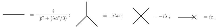
Figure 3.1: Feynman rules at $\phi_{0}=a$

Let us take a closer look at the case of small tadpoles, that is naturally amenable to a perturbative treatment. This can illustrate a further important subtlety: the diagrams that contribute to this series are not all 1PI, and thus by the usual rules should not all contribute to $\Gamma$. For instance, let us consider the Lagrangian

$${\cal L}\ =\ -\,\frac{1}{2}\,(\partial_{\mu}\phi)^{2}\ -\ \frac{\lambda}{4!}(\phi^{2}-a^{2})^{2}\ +\ c\;\phi\ ,$$ (3.22)

with a Mexican-hat section potential and a driving “magnetic field” represented by the tadpole $c$. The issue is to single out the terms produced in the gaussian expansion of the path integral of eq. (3.22) once the integration variable is shifted about the “wrong” vacuum $\phi_{0}=a$, writing $\phi=a+\chi$, so that

$$e^{\frac{i}{\hbar}\,W[J]}\ =\int[D\phi]\ e^{\frac{i}{\hbar}\int d^{\cal D}x\left(\;-\;\frac{1}{2}\partial_{\mu}\chi\partial^{\mu}\chi\,-\,\frac{\lambda a^{2}}{6}\chi^{2}\,-\,\frac{\lambda a}{3!}\chi^{3}\,-\,\frac{\lambda}{4!}\chi^{4}\,+\,c(a+\chi)\,+\,J(a+\chi)\right)}\ .$$ (3.23)

Notice that, once $\chi$ is rescaled to $\hbar^{1/2}\chi$ in order to remove all powers of $\hbar$ from the gaussian term, in addition to the usual positive powers of $\hbar$ associated to cubic and higher terms, a negative power $\hbar^{-1/2}$ accompanies the tadpole term in the resulting Lagrangian. As a result, the final ${\cal O}(1/\hbar)$ contribution that characterizes the classical vacuum energy results from infinitely many diagrams built with the Feynman rules summarized in fig. 3.1. The first two non-trivial contributions originate from the three-point vertex terminating on three tadpoles, from the four-point vertex terminating on four tadpoles and from the exchange diagram of fig. 3.2.

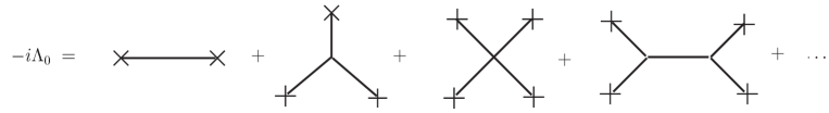
Figure 3.2: Vacuum energy

As anticipated, tadpoles affect substantially the character of the diagrams contributing to $\Gamma$, and in particular to the vacuum energy, that we shall denote by $\Lambda_{0}$. Beginning from the latter, let us note that, in the presence of a tadpole coupling $c$,

$$e^{-\frac{i}{\hbar}\Lambda_{0}\,{\cal V}}\ =\ \int[D\phi]\ e^{\frac{i}{\hbar}\left(S[\phi]\,+\,\int d^{\cal D}x\;c\phi\right)}\ ,$$ (3.24)

where ${\cal V}$ denotes the volume of space time. Hence, the vacuum energy is actually determined by a power series in $c$ whose coefficients are connected, rather than 1PI, amplitudes, since they are Green functions of W computed for a classical value of the current determined by $c$:

$$-\,\frac{i}{\hbar}\,\Lambda_{0}\,{\cal V}\ =\ \sum_{n}\ \frac{(i\;c)^{n}}{n!\;\hbar^{n}}\ W^{(n)}[\{p_{j}=0\}]\ .$$ (3.25)

A similar argument applies to the higher Green functions of $\Gamma$: the standard Legendre transform becomes effectively in this case

$$W[J+c]\ =\ \Gamma[\bar{\phi}]\ +\ J\bar{\phi}\ ,$$ (3.26)

since the presence of a tadpole shifts the argument of W. However, the l.h.s. of (3.26) contains an infinite series of conventional connected Green functions, and after the Legendre transform only those portions that do not depend on the tadpole $c$ are turned into 1PI amplitudes. The end conclusion is indeed that the contributions to $\Gamma$ that depend on the tadpoles involve arbitrary numbers of connected, but also non 1PI, diagrams.

The vacuum energy is a relatively simple and most important quantity that one can deal with from this viewpoint, and its explicit study will help to clarify the meaning of eq. (3.19). Using eqs. (3.14) and (3.16) one can indeed conclude that, at the classical level,

$$\Lambda_{0}\ =\ -\,\frac{W(J=0)}{\cal V}\ =\ -\,V(\phi_{0})\ -\ \frac{i}{2}\ \Delta\,\left.{\cal D}\right|_{p^{2}=0}\Delta+{\cal O}(\Delta^{3})\ ,$$ (3.27)

an equation that we shall try to illustrate via a number of examples in this Chapter. The net result of this Section is that resummations around a wrong vacuum lead nonetheless to extrema of the effective action. However, it should be clear from the previous derivation that the scalar propagator must be nonsingular, or equivalently the potential must not have an inflection point at $\phi_{0}$, in order that the perturbative corrections about the original wrong vacuum be under control. A related question is whether the resummation flow converges generically towards minima (local or global) or can end up in a maximum. As we shall see in detail shortly, the end point is generally an extremum and not necessarily a local minimum.

3.3 The end point of the resummation flow

The purpose of this Section is to investigate, for some explicit forms of the scalar potential $V(\phi)$ and for arbitrary initial values of the scalar field $\phi_{0}$, the end point reached by the system after classical tadpole resummations are performed. The answer, that will be justified in a number of examples, is as follows: starting from a wrong vacuum $\phi_{0}$, the system typically reaches a nearby extremum (be it a minimum or a maximum) of the potential not separated from it by any inflection. While this is the generic behavior, we shall also run across a notable exception to this simple rule: there exist some peculiar “large” flows, corresponding to special values of $\phi_{0}$, that can actually reach an extremum by going past an inflection, and in fact even crossing a barrier, but are nonetheless captured by the low orders of the perturbative expansion!

An exponential potential is an interesting example that is free of such inflection points, and is also of direct interest for supersymmetry breaking in String Theory. Let us therefore begin by considering a scalar field with the Lagrangian

$${\cal L}\ =\ -\,\frac{1}{2}\,\partial^{\mu}\phi\,\partial_{\mu}\phi\ -\ \alpha\ e^{b\phi}\ ,$$ (3.28)

where for definiteness the two coefficients $\alpha$ and $b$ are both taken to be positive. The actual minimum is reached as $\phi\to-\infty$, where the classical vacuum energy vanishes.

In order to recover this result from a perturbative expansion around a generic “wrong” vacuum $\phi_{0}$, let us shift the field, writing $\phi=\phi_{0}+\chi$. The Feynman rules can then be extracted from

$${\cal L}_{eff}=-\,\frac{1}{2}\ \partial^{\mu}\chi\,\partial_{\mu}\chi\ -\ \frac{\Delta}{b}\ e^{b\chi}\ ,$$ (3.29)

where $\Delta$, the one-point function in the “wrong” vacuum, is defined by

$$-\ \left.\frac{\delta{\cal L}_{eff}}{\delta\phi}\right|_{\phi_{0}}\ =\ \Delta\ =\ \alpha\ b\ e^{b\phi_{0}}\ ,$$ (3.30)

and the first few contributions to the classical vacuum energy are as in fig. 3.3.

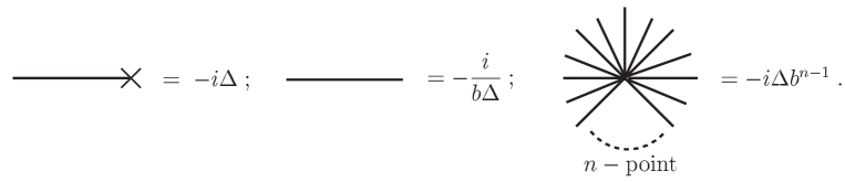
Figure 3.3: Feynman rules for the exponential potential

It is fairly simple to compute the first few diagrams. For instance, the two-tadpole correction to $-iV(\phi_{0})$ is

$$\ \frac{1}{2}\ \frac{-i}{b\Delta}\ (-i\Delta)^{2}=-\frac{1}{2}\left(\frac{-i\Delta}{b}\right)\ ,$$ (3.31)

while the three-tadpole correction, still determined by a single diagram, is

$$\frac{1}{3!}\ (-i\Delta\ b^{2})\ (-i\Delta)^{3}\left(\frac{-i}{b\Delta}\right)^{3}\ =\ -\ \frac{1}{6}\left(\frac{-i\Delta}{b}\right)\ .$$ (3.32)

On the other hand, the quartic contribution is determined by two distinct diagrams, and equals

$$\frac{1}{4!}\ (-i\Delta\ b^{3})\ (-i\Delta)^{4}\left(\frac{-i}{b\Delta}\right)^{4}+\frac{1}{8}\ (-i\Delta\ b^{2})^{2}\ (-i\Delta)^{4}\left(\frac{-i}{b\Delta}\right)^{5}\ =\ -\ \frac{1}{12}\left(\frac{-i\Delta}{b}\right)\ ,$$ (3.33)

while the quintic contribution originates from three diagrams. Putting it all together, one obtains

$$\Lambda_{0}\ =\ \frac{\Delta}{b}\ \left(1-\frac{1}{2}-\frac{1}{6}-\frac{1}{12}-\frac{1}{20}+\ldots\right)\ =\ \frac{\Delta}{b}\left[1-\sum_{n=1}^{\infty}\frac{1}{n(n+1)}\right]\ .$$ (3.34)

The resulting pattern is clearly identifiable, and suggests in an obvious fashion the series in (3.34). Notice that, despite the absence of a small expansion parameter, in this example the series in (3.34) actually converges to $1$, so that the correct vanishing value for the classical vacuum energy can be exactly recovered from an arbitrary wrong vacuum $\phi_{0}$.

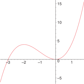
Figure 3.4: A cubic potential

We can now turn to a more intricate example and consider the model

$${\cal L}\ =\ -\,\frac{1}{2}(\partial_{\mu}\phi)^{2}\ -\ \frac{m^{2}\phi^{2}}{2}\ -\ \frac{\lambda\phi^{3}}{6}\ ,$$ (3.35)

the simplest setting where one can investigate the role of an inflection. Strictly speaking this example is pathological, since its Hamiltonian is unbounded from below, but for our purpose of gaining some intuition on classical resummations it is nonetheless instructive. The two extrema of the scalar potential $v_{1,2}$ and the inflection point $v_{I}$ are

$$v_{1}=0\ ,\quad v_{2}=-\frac{2m^{2}}{\lambda}\ ,\quad v_{I}=-\frac{m^{2}}{\lambda}\ .$$ (3.36)

Starting from an arbitrary initial value $\phi_{0}$, let us investigate the convergence of the resummation series and the resulting resummed value $\langle\phi\rangle$. A close look at the diagrammatic expansion indicates that

$$\langle\phi\rangle\ =\ \phi_{0}+\ \frac{V^{\prime}}{V^{{}^{\prime\prime}}}\ \sum_{n=0}^{\infty}c_{n}\left[\frac{\lambda V^{\prime}}{(V^{{}^{\prime\prime}})^{2}}\right]^{n}\ \equiv\ \phi_{0}+\frac{V^{\prime}}{V^{{}^{\prime\prime}}}\ f(x)\ ,$$ (3.37)

where the actual expansion variable is

$$x\ =\ \frac{\lambda V^{\prime}}{(V^{{}^{\prime\prime}})^{2}}\ ,$$ (3.38)

to be contrasted with the naive dimensionless expansion variable

$$z=\frac{\lambda\phi_{0}}{m^{2}}\ .$$ (3.39)

According to eq. (3.38), their relation is

$$x=\frac{z(z+2)}{2(z+1)^{2}}\ ,$$ (3.40)

whose inverse is

$$z=-1\ \mp\ \frac{1}{\sqrt{1-2x}}\ ,$$ (3.41)

where the upper sign corresponds to the region $(L)$ to the left of the inflection, while the lower sign corresponds to the region $(R)$ to the right of the inflection. In other words: $\phi_{0}$, and thus the naive variable $z$ of the problem, is actually a double-valued function of $x$, while the actual range covered by $x$ terminates at the inflection.

A careful evaluation of the symmetry factors of various diagrams with variable numbers of tadpole insertions shows that

$$f(x)\ =\ -\,\frac{\sqrt{\pi}}{2}\sum_{n=0}^{\infty}\frac{(-1)^{n}\ 2^{n+1}}{(n+1)!\ \Gamma{(1/2-n)}}\ x^{n}\ ,$$ (3.42)

a series that for $|x|<1/2$ converges to

$$f(x)\ =\ -\,\frac{1}{x}\ +\ \frac{\sqrt{1-2x}}{x}\ .$$ (3.43)

The relation between $z$ and $x$ implies that both $\phi_{0}$ and $V^{{}^{\prime\prime}}$ have two different expressions in terms of $x$ on the two sides of the inflection,

$$V^{{}^{\prime\prime}}=\pm\frac{m^{2}}{\sqrt{1-2x}}\quad,\quad\phi_{0}=-\frac{m^{2}}{\lambda}\mp\frac{m^{2}}{\lambda}\frac{1}{\sqrt{1-2x}}\ ,$$ (3.44)

where the upper signs apply to the region $(L)$ that lies to the left of the inflection, while the lower signs apply to the region $(R)$ that lies to the right of the inflection. Combining (3.43) and (3.44) finally yields the announced result:

$$\langle\phi\rangle\rightarrow 0\quad{\rm in\ the\ (R)\ region:}\quad-\frac{m^{2}}{\lambda}<\phi_{0}<\infty\ ,$$

$$\langle\phi\rangle\rightarrow-\frac{2m^{2}}{\lambda}\quad{\rm for\ in\ (L)\ region:}\quad-\infty<\phi_{0}<-\frac{m^{2}}{\lambda}\ .$$ (3.45)

The resummation clearly breaks down near the inflection point $v_{I}$. In the present case, the series in (3.43) converges for $|x|<1/2$, and this translates into the condition

$$\phi_{0}\in\left(-\infty,-\frac{m^{2}}{\lambda}\left(1+\frac{1}{\sqrt{2}}\right)\right)\ \bigcup\ \left(-\frac{m^{2}}{\lambda}\left(1-\frac{1}{\sqrt{2}}\right),\infty\right)\ .$$ (3.46)

A symmetric interval around the inflection point thus lies outside this region, while in the asymptotic regions $\phi_{0}\rightarrow\pm\infty$ the parameter $x$ tends to $1/2$, a limiting value for the convergence of the series (3.42).

The vacuum energy $\Lambda_{0}$ is another key quantity for this problem. Starting as before from an arbitrary initial value $\phi_{0}$, standard diagrammatic methods indicate that

$$\Lambda_{0}=\ V(\phi_{0})+\ \frac{(V^{\prime})^{2}}{V^{{}^{\prime\prime}}}\ \sum_{n=0}^{\infty}d_{n}\left[\frac{\lambda V^{\prime}}{(V^{{}^{\prime\prime}})^{2}}\right]^{n}\ \equiv\ V(\phi_{0})+\frac{(V^{\prime})^{2}}{V^{{}^{\prime\prime}}}\ h(x)\ .$$ (3.47)

A careful evaluation of the symmetry factors of various diagrams with arbitrary numbers of tadpole insertions then shows that

$$h(x)\ =\ -\,\frac{\sqrt{\pi}}{4}\sum_{n=0}^{\infty}\frac{(-1)^{n}\ 2^{n+2}}{(n+2)!\ \Gamma{(1/2-n)}}\ x^{n}\ ,$$ (3.48)

that for $|x|<1/2$ converges to

$$h(x)\ =\ \frac{1}{3x^{2}}\left[1-3x-(1-2x)^{3/2}\right]\ .$$ (3.49)

The two different relations between $z$ and $x$ in (3.41) that apply to the two regions $(L)$ and $(R)$ finally yield:

$$\Lambda_{0}\rightarrow 0\ ,\quad{\rm in\ the\ (R)\ region}\ -\frac{m^{2}}{\lambda}<\phi_{0}<\infty\ ,$$

$$\Lambda_{0}\rightarrow\frac{2m^{6}}{3\lambda^{2}}\ ,\quad{\rm in\ the\ (L)\ region}\ -\infty<\phi_{0}<-\frac{m^{2}}{\lambda}\ .$$ (3.50)

To reiterate, we have seen how in this model the resummations approach nearby extrema (local minima or maxima) not separated from the initial value $\phi_{0}$ by any inflection.

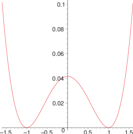
Figure 3.5: A quartic potential

A physically more interesting example is provided by a real scalar field described by the Lagrangian

$${\cal L}\ =\ -\,\frac{1}{2}(\partial_{\mu}\phi)^{2}\ -\ \frac{\lambda}{4!}\;(\phi^{2}-a^{2})^{2}\ ,$$ (3.51)

whose potential has three extrema, two of which are a pair of degenerate minima, $v_{1}=-a$ and $v_{3}=+a$, separated by a potential wall, while the third is a local maximum at the origin. Two inflection points are now present,

$$v^{(1)}_{I}=-\frac{a}{\sqrt{3}}\ ,\qquad v^{(2)}_{I}=\frac{a}{\sqrt{3}}\ ,$$ (3.52)

that also form a symmetric pair with respect to the vertical axis.

Starting from an arbitrary initial value $\phi_{0}$, one can again in principle sum all the diagrams, and a closer look shows that there are a pair of natural variables, $y_{1}$ and $y_{2}$, defined as

$$y_{1}\ =\ \phi_{0}\ \frac{\lambda V^{\prime}}{(V^{{}^{\prime\prime}})^{2}}\qquad{\rm and}\qquad y_{2}\ =\ \frac{\lambda{V^{\prime}}^{2}}{(V^{{}^{\prime\prime}})^{3}}\ ,$$ (3.53)

that reflect the presence of the cubic and quartic vertices and depend on the square of $\phi_{0}$. On the other hand, the naive dimensionless variable to discuss the resummation flow is in this case

$$z=\phi_{0}^{2}/{a}^{2}\ ,$$ (3.54)

and eqs. (3.53) imply that

$$y_{1} = 6\,\frac{z(z-1)}{(3z-1)^{2}}\ ,$$ (3.55)

$$y_{2} = 6\,\frac{z(z-1)^{2}}{(3z-1)^{3}}\ .$$ (3.56)

The diagrammatic expansions of $\langle\phi\rangle$ and $\Lambda_{0}$ are now more complicated than in the $\phi^{3}$ example. A careful evaluation of the symmetry factors of various diagrams, however, uncovers an interesting pattern, since

$$\langle\phi\rangle = \phi_{0}+\frac{V^{\prime}}{V^{{}^{\prime\prime}}}\left[-1-\frac{1}{2}\left(y_{1}-\frac{y_{2}}{3}\right)-\frac{1}{2}\left(y_{1}-\frac{y_{2}}{3}\right)\left(y_{1}-\frac{y_{2}}{2}\right)\right.$$

$$- \left.\frac{5}{8}\left(y_{1}-\frac{y_{2}}{3}\right)\left(y_{1}-\frac{2y_{2}}{3}\right)\left(y_{1}-\frac{2y_{2}}{5}\right)\right.$$

$$- \left.\frac{7}{8}\left(y_{1}-\frac{y_{2}}{3}\right)\left(y_{1}^{3}-\frac{5}{3}y_{1}^{2}y_{2}+\frac{55}{63}y_{1}y_{2}^{2}-\frac{55}{378}y_{2}^{3}\right)\right.$$

$$- \frac{21}{16}\ \left.\left(y_{1}-\frac{y_{2}}{3}\right)\left(y_{1}^{4}-\frac{16}{7}y_{1}^{3}y_{2}+\frac{13}{7}y_{1}^{2}y_{2}^{2}-\frac{52}{81}y_{1}y_{2}^{3}+\frac{13}{162}y_{2}^{4}\right)+\cdots\right]\ ,$$

$$\Lambda_{0} = V(\phi_{0})+\frac{(V^{\prime})^{2}}{V^{{}^{\prime\prime}}}\left[-\frac{1}{2}-\frac{1}{6}\left(y_{1}-\frac{y_{2}}{4}\right)-\frac{1}{8}\left(y_{1}-\frac{y_{2}}{3}\right)^{2}\right.$$ (3.57)

$$- \left.\frac{1}{8}\left(y_{1}-\frac{y_{2}}{3}\right)^{2}\left(y_{1}-\frac{1}{2}y_{2}\right)-\frac{7}{48}\left(y_{1}-\frac{y_{2}}{3}\right)^{2}\,\left(y_{1}^{2}-\frac{22}{21}y_{1}y_{2}+\frac{11}{42}y_{2}^{2}\right)\right.$$

$$- \left.\frac{3}{16}\left(y_{1}-\frac{y_{2}}{3}\right)^{2}\left(y_{1}^{3}-\frac{13}{8}y_{1}^{2}y_{2}+\frac{91}{108}y_{1}y_{2}^{2}-\frac{91}{648}y_{2}^{3}\right)+\cdots\right]\ ,$$

where all linear and higher-order corrections in $\langle\phi\rangle$ and all quadratic and higher order corrections in $\Lambda_{0}$ apparently disappear at the special point $y_{1}=y_{2}/3$. Notice that this condition identifies the three extrema $\phi_{0}=\pm a$ and $\phi_{0}=0$, but also, rather surprisingly, the two additional points $\phi_{0}=\pm\frac{a}{2}$. In all these cases the series expansions for $\langle\phi\rangle$ and $\Lambda_{0}$ apparently end after a few terms.

If one starts from a wrong vacuum sufficiently close to one of the extrema, one can convince oneself that, in analogy with the previous example,

$$\langle\phi\rangle\rightarrow-a\quad,\quad{\rm for\ region\ 1:}\quad-\infty<\phi_{0}<v^{(1)}_{I}\ ,$$

$$\langle\phi\rangle\rightarrow 0\quad,\quad{\rm for\ region\ 2:}\quad v^{(1)}_{I}<\phi_{0}<v^{(2)}_{I}\ ,$$

$$\langle\phi\rangle\rightarrow+a\quad,\quad{\rm for\ region\ 3:}\quad v^{(2)}_{I}<\phi_{0}<\infty\ ,$$ (3.58)

but we have not arrived at a single natural expansion parameter for this problem, an analog of the variable $x$ of the cubic potential. In addition, while these perturbative flows follow the pattern of the previous example, since they are separated by inflections that act like barriers, a puzzling and amusing result concerns the special initial points

$$\phi_{0}=\pm\frac{a}{2}\ .$$ (3.59)

In this case $y_{2}=3y_{1}$ and, as we have seen, apparently all but the first few terms in $\langle\phi\rangle$ and all but the first few terms in $\Lambda_{0}$ vanish. The non-vanishing terms in eq. (3.57) show explicitly that the endpoints of these resummation flows correspond to $\langle\phi\rangle=\pm a$ for $\phi_{0}=\mp\frac{a}{2}$, and that $\Lambda_{0}=0$, so that these two flows apparently “cross” the potential barrier and pass beyond an inflection. One might be tempted to dismiss this phenomenon, since after all this is a case with large tadpoles (and large values of $y_{1}$ and $y_{2}$), that is reasonably outside the region of validity of perturbation theory and hence of the strict range of applicability of eq. (3.57). Still, toward the end of this Section we shall encounter a similar phenomenon, clearly within a perturbative setting, where the resummation will unquestionably collapse to a few terms to land at an extremum, and therefore it is worthwhile to pause and devote to this issue some further thought.

Interestingly, the tadpole resummations that we are discussing have a simple interpretation in terms of Newton’s method of tangents, a very effective iterative procedure to derive the roots of non-linear algebraic equations. It can be simply adapted to our case, considering the function $V^{\prime}(\phi)$, whose zeroes are the extrema of the scalar potential. The method begins with guess, a “wrong vacuum” $\phi_{0}$, and proceeds via a sequence of iterations determined by the zeros of the sequence of straight lines

$$y-V^{\prime}(\phi^{(n)})\ =\ V^{{}^{\prime\prime}}(\phi^{(n)})\ (x-\phi^{(n)})\ ,$$ (3.60)

that are tangent to the curve at subsequent points, defined recursively as

$$\phi^{(n+1)}\ =\ \phi^{(n)}\ -\ \frac{V^{\prime}(\phi^{(n)})}{V^{{}^{\prime\prime}}(\phi^{(n)})}\ ,$$ (3.61)

where $\phi^{(n)}$ denotes the $n$-th iteration of the wrong vacuum $\phi^{(0)}=\phi_{0}$.

When applied to our case, restricting our attention to the first terms the method gives

$$\phi^{(1)} = \phi_{0}-\frac{V^{\prime}}{V^{{}^{\prime\prime}}}\ ,$$

$$\phi^{(2)} = \phi^{(1)}-\frac{V^{\prime}(\phi^{(1)})}{V^{{}^{\prime\prime}}(\phi^{(1)})}=\phi_{0}+\frac{V^{\prime}}{V^{{}^{\prime\prime}}}\left[\,-1\ -\ \frac{\frac{V^{\prime}\;V^{{}^{\prime\prime\prime}}}{2(V^{{}^{\prime\prime}})^{2}}-\frac{(V^{\prime})^{2}\;V^{{}^{\prime\prime\prime\prime}}}{6(V^{{}^{\prime\prime}})^{3}}}{1-\frac{V^{\prime}V^{{}^{\prime\prime\prime}}}{(V^{{}^{\prime\prime}})^{2}}+\frac{(V^{\prime})^{2}V^{{}^{\prime\prime\prime\prime}}}{2(V^{{}^{\prime\prime}})^{3}}}\,\right]$$ (3.62)

$$\cong \phi_{0}+\frac{V^{\prime}}{V^{{}^{\prime\prime}}}\biggl{[}-1-\frac{1}{2}(y_{1}-\frac{y_{2}}{3})-\frac{1}{2}(y_{1}-\frac{y_{2}}{3})(y_{1}-\frac{y_{2}}{2})\biggr{]}\ ,$$

where $y_{1}$ and $y_{2}$ are defined in (3.53) and, for brevity, the arguments are omitted whenever they are equal to $\phi_{0}$. Notice the precise agreement with the first four terms in (3.57), that imply that our tadpole resummations have a simple interpretation in terms of successive iterations of the solutions of the vacuum equations $V^{\prime}=0$ by Newton’s method. Notice the emergence of the combination $y_{1}-y_{2}/3$ after the first iteration: as a result, the pattern of eqs. (3.57) continues indeed to all orders.

In view of this interpretation, the non-renormalization points $\phi_{0}=\pm a/2$ acquire a clear geometrical interpretation: in these cases the iteration stops after the first term $\phi^{(1)}$, since the tangent drawn at the original “wrong” vacuum, say at $a/2$, happens to cross the real axis precisely at the extremum on the other side of the barrier, at $\langle\phi\rangle=-a$. Newton’s method can also shed some light on the behavior of the iterations, that stay on one side of the extremum or pass to the other side according to the concavity of the potential, and on the convergence radius of our tadpole resummations, that the second iteration already restricts $y_{1}$ and $y_{2}$ to the region

$$\left|y_{1}\ -\ \frac{y_{2}}{2}\right|\ <\ 1\ .$$ (3.63)

However, the tangent method behaves as a sort of Dyson resummation of the naive diagrammatic expansion, and has therefore better convergence properties. For instance, starting near the non-renormalization point $\phi_{0}\simeq-a/2$, the first iteration lands far away, but close to the minimum $\phi^{(1)}\simeq a$. The second correction, that when regarded as a resummation in (3.57) is large, is actually small in the tangent method, since it is proportional to $(1/16)(y_{1}-y_{2}/3)$. It should be also clear by now that not only the points $\phi_{0}=\pm a/2$, but finite intervals around them, move across the barrier as a result of the iteration. These steps, however, do not have a direct interpretation in terms of Feynman diagram tadpole resummations, since (3.63) is violated, so that the corresponding diagrammatic expansion actually diverges. The reason behind the relative simplicity of the cubic potential (3.35) is easily recognized from the point of view of the tangent method: the corresponding $V^{\prime}(\phi)$ is a parabola, for which Newton’s method never leads to tangents crossing the real axis past an inflection point.

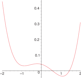
Figure 3.6: A quartic potential with a “magnetic” deformation

There is a slight technical advantage in returning to the example of eq. (3.22), since for a small magnetic field (tadpole) $c$ one can expand the complete expressions for the vacuum energy and the scalar v.e.v.’s in powers of the tadpole. The expansions (3.57) still apply, with an obvious change in the one-point function $V^{\prime}$, and their sums should coincide, term by term, with the tadpole resummations obtained starting from the undeformed “wrong” vacua $\phi_{0}=\pm a,0$.

In this case the vacuum energy is given by

$$\Lambda_{0}\ =\ \frac{\lambda}{4!}\,(v^{2}-a^{2})^{2}\ -\ c\;v\ ,$$ (3.64)

where the correct vacuum value $\langle\phi\rangle=v$ is determined by the cubic equation

$$\lambda\frac{v}{6}\;(v^{2}-a^{2})\ -\ c\ =\ 0\ ,$$ (3.65)

that can be easily solved perturbatively in the tadpole $c$, so that if one starts around $\phi_{0}=a$,

$$\Lambda_{0}\ =\ -\,c\;a\ -\ \frac{3c^{2}}{2\lambda a^{2}}\ +\ {\cal O}(c^{3})\ .$$ (3.66)

This result can be also recovered rather simply starting from the wrong vacuum $\phi_{0}=a$ and making use of eq. (3.27), since in this case $\Delta=-c$ and ${\cal D}(p^{2}=0)=-3i/\lambda a^{2}$. However, the cubic equation (3.65) can be also solved exactly in terms of radicals, and in the small tadpole limit its three solutions are real and can be written in the form

$$v\ =\ \frac{2a}{\sqrt{3}}\ \cos\left[\frac{\alpha}{3}+\frac{2\pi k}{3}\right]\qquad(k=0,1,2)\ ,$$ (3.67)

where

$$\cos(\alpha)=\xi\ ,\qquad\sin(\alpha)=\sqrt{1-\xi^{2}}\ ,\quad{\rm with}\quad\xi=\frac{9\sqrt{3}c}{\lambda a^{3}}\ .$$ (3.68)

For definiteness, let us consider a tadpole $c$ that is small and positive, so that the absolute minimum of the deformed potential lies in the vicinity of the original minimum of the Mexican-hat section at $v=a$ and corresponds to $k=0$. We can now describe the fate of the resummations that start from two different wrong vacua:

i) $\phi_{0}=a$. In this case and in the small tadpole limit $\xi<<1$ resummations in the diagrammatic language produce the first corrections

$$\langle\phi\rangle=a+\frac{3c}{\lambda a^{2}}-\frac{27c^{2}}{2\lambda^{2}a^{5}}+\cdots\ .$$ (3.69)

Alternatively, this result could be obtained solving eq. (3.65) in powers of the tadpole $c$ with the initial value $\phi_{0}=a$, so that, once more, starting from a wrong vacuum close to an extremum and resumming one can recover the correct answer order by order in the expansion parameter. In this case both a cubic and a quartic vertex are present, and the complete expression for the vacuum energy, obtained substituting (3.67) in (3.64), is

$$\Lambda_{0}\ =\ \frac{2\;\lambda a^{4}\;\xi}{27}\ \left[\frac{\xi}{16}\,\frac{1}{\cos^{2}\left(\frac{\alpha}{3}\right)}\ -\ \cos\left(\frac{\alpha}{3}\right)\right]\ .$$ (3.70)

This can be readily expanded in a power series in $\xi$, whose first few terms,

$$\Lambda_{0}\ =\ -a\;c\ -\ \frac{\sqrt{3}}{18}\;a\;c\;\xi\ +\ \frac{1}{54}\;a\;c\;\xi^{2}\ -\ \frac{\sqrt{3}}{243}\;a\;c\;\xi^{3}\ +\ {\cal O}(\xi^{4})\ .$$ (3.71)

match precisely the tadpole expansion (3.57).

ii) $\phi_{0}=0$. In this case the first corrections obtained resumming tadpole diagrams are

$$\langle\phi\rangle=-\frac{6c}{\lambda a^{2}}-\frac{216c^{3}}{\lambda^{3}a^{8}}+\cdots\ .$$ (3.72)

The same result can be obtained expanding the solution of (3.65) in powers of the tadpole $c$, starting from the initial value $\phi_{0}=0$. We can now compare (3.67) with (3.57), noting that in this case only the quartic vertex is present, so that $y_{1}=0$. Since $y_{2}=-8\xi^{2}/9$ for $\phi_{0}=0$, the v.e.v. $\langle\phi\rangle$ contains only odd powers of the tadpole $c$, a property that clearly holds in (3.67) as well, since $\xi\rightarrow-\xi$ corresponds to $\alpha\rightarrow\alpha+(2l+1)3\pi$, with $l$ integer and $v\rightarrow-v$ in (3.67). The contributions to $\langle\phi\rangle$ are small and negative, and therefore, starting from a wrong vacuum close to a maximum of the theory, the resummation flow leads once more to a nearby extremum (the local maximum slightly to the left of the origin, in this case), rather than rolling down to the minimum corresponding to the $k=0$ solution of (3.67). The important points in the scalar potential are again the extrema and the inflections, precisely as we had seen in the example with a cubic potential. Barring the peculiar behavior near the points identified by the condition $y_{1}=y_{2}/3$, the scalar field flows in general to the nearest extremum (minimum or maximum) of this potential, without passing through any inflection point along the whole resummation flow. It should be appreciated how the link with Newton’s method associates a neat geometrical interpretation to this behavior.

For $\xi=1$ the two extrema of the unperturbed potential located at $\ v=-a\$ and at $\ v=0\$ coalesce with the inflection at $-a/\sqrt{3}$. If the potential is deformed further, increasing the value of the tadpole, the left minimum disappears and one is left with only one real solution, corresponding to $k=0$. The correct parametrization for $\ \xi>1\$ is $\ \cosh(\alpha)=\xi\$ and $\ \sinh(\alpha)=\sqrt{\xi^{2}-1}\$, and the classical vacuum energy is like in (3.70), but with $\ \cos(\alpha/3)$ replaced by $\cosh(\alpha/3)$. In order to recover the result (3.71) working perturbatively in the “wrong” vacuum $v=a$, one should add the contributions of an infinite series of diagrams that build a power series in $1/\xi$, but this cannot be regarded as a tadpole resummation anymore. The meaning of the parameter $\xi$ should by now have become apparent: it is proportional to the product of the tadpole and the propagator in the wrong vacuum, $V^{\prime}/V^{\prime\prime}$, a natural expansion parameter for problems of this type. Notice that the ratio $V^{\prime}/V^{{}^{\prime\prime}}$ is twice as large (and of opposite sign) at the origin $\phi_{0}=0$ than at $\phi_{0}=a$. Therefore, the tadpole expansion first breaks down around $\phi_{0}=0$. As we have seen, the endpoint of the resummation flow for $\phi_{0}=0$ is the local maximum corresponding to $k=2$ in (3.67), that is reached for $\xi<1$. At $\xi=1$, however, the two extrema corresponding to $k=1$ and $k=2$ coalesce with the inflection at $-a/\sqrt{3}$, and hence there is no possible endpoint for the resummation flow. This is transparent in (3.67), since for $\xi\geq 1$ the $\xi$ expansion clearly breaks down. It should therefore be clear why, if the potential is deformed too extensively, corresponding to $\ \xi>1$, a perturbative expansion around the extrema $\ v=\pm a,0\$ in powers of $\xi$ is no longer possible. Another key issue that should have emerged from this discussion is the need for an independent, small expansion parameter when tadpoles are to be treated perturbatively. In this example, as anticipated, the expansion parameter $\xi$ can be simply related to the potential according to

$$\xi\ =\ \frac{3\sqrt{3}}{a}\ \left|\frac{V^{\prime}}{V^{\prime\prime}}\right|\ ,$$ (3.73)

that is indeed small if $c$ is small.

It is natural to ask about the fate of the points $\phi_{0}=\pm a/2$ of the previous example (3.51) when the magnetic field $c$ is turned on. Using the parameters $y_{i}$ in (3.53), the condition determining these special points, $y_{1}=y_{2}/3$, is equivalent to

$$V^{\prime}\ =\ 3\ \phi_{0}\ V^{{}^{\prime\prime}}\ .$$ (3.74)

It is readily seen that the solutions of this cubic equation are precisely $\phi_{0}=-v/2$, if $v$ denotes, collectively, the three extrema solving (3.65). Hence, in this case $\langle\phi\rangle=-2\phi_{0}=v$, confirming the persistence of these non-renormalization points. In the present case, however, there is a third non-renormalization point, $\phi_{0}=-v_{k=2}/2$, that for small values of $\xi$ is well inside the convergence region. This last point clearly admits an interpretation in terms of tadpole resummations, and the possible existence of effects of this type in String Theory raises the hope that explicit vacuum redefinitions could be constructed in a few steps for special values of the string coupling and of other moduli.

3.3.1 On Newton’s Tangent Method and the Quartic Potential

It is actually simple to prove that, if one starts with $\phi_{0}$ in region 1, one ends up in the vacuum $<\phi>=-a$, while if one starts in region 3 one ends up in $<\phi>=+a$, without ever crossing the barrier. This is due to the fact that the function $V^{\prime}$ is convex in those regions, and that at the corresponding extrema it has opposite signs. This implies that there is only one zero, and that Newton’s series converges to it. On the other hand region 2, to which we now turn, is far richer, even though, in some sense, it is “non-perturbative”. Hence, our discussion will rely directly on Newton’s method, but will be only loosely related to the conventional field theory expansion.

The inflections are “initial points” where the series clearly diverges, since $V^{\prime\prime}$ vanishes there. If we enter region 2 and move to the left of $a/\sqrt{3}$ (of course, going to the right of $-a/\sqrt{3}$ would lead to very similar results), the first iteration falls in region 1, while the successive ones lead inevitably to $<\phi>=-a$. Therefore, in this case Newton’s method leads to barrier crossing, and this happens until one hits a point that we will call of the “y-class”, that we shall denote by $y_{1}$. Starting from this point, the first iteration crosses the barrier and hits the $\phi$-axis exactly at $-a/\sqrt{3}$. $y_{1}$ solves the equation

$$2\sqrt{3}x^{3}+3ax^{2}-a^{3}=0\qquad.$$

Hence, after the first iteration, $y_{1}$ leads to a divergence. The region ${\cal Y}_{1}=\{y_{1}<\phi_{0}<a/\sqrt{3}\}$ is therefore the first “barrier-crossing” region: starting there, one ends up on the opposite side, at $<\phi>=-a$. This region, in particular, contains the “non renormalization point” $a/2$, that solves the equation

$$2x^{3}+3ax^{2}-a^{3}=0\qquad.$$

Moving to the left of $y_{1}$, another region opens up. This can be seen noticing that the first iteration intersects the $\phi$-axis to the right of $-a/\sqrt{3}$, in such a way that the second iteration ends inevitably inside region 3. Consequently, Newton’s method now leads to $<\phi>=+a$ after an infinite number of steps and after crossing the barrier. Again, this happens until one hits a point, that we will call of the “z-class”, say $z_{1}$, such that the second iteration exactly intersects the $\phi$-axis at the point $a/\sqrt{3}$, bringing again to a divergence. It should be noticed that the region ${\cal Z}_{1}=\{z_{1}<\phi_{0}<y_{1}\}$ is again of “barrier-crossing type” (or, better, of “bouncing type”), but the final vacuum is now $<\phi>=+a$. It can also be thought of as the region such that, after the first iteration, leads exactly to the opposite of ${\cal Y}_{1}$ region, because the iteration of $z_{1}$ falls exactly, by definition, onto $-y_{1}$.

The nature of the iterative procedure should now be apparent: moving to the left of $z_{1}$, one meets another “y-class” region, ${\cal Y}_{2}=\{y_{2}<\phi_{0}<z_{1}\}$, where $y_{2}$ now leads exactly to $y_{1}$ after two iterations, and to the left inflexion point $-a/\sqrt{3}$ after three iterations. To the left of $y_{2}$, there is the second “z-class” region, ${\cal Z}_{2}=\{z_{2}<\phi_{0}<y_{2}\}$, where $z_{2}$ falls on $z_{1}$ after two iterations, and on the inflection point $a/\sqrt{3}$ after four iterations, and so on. There is hence a countable infinity of “y-class” regions ${\cal Y}_{n}=\{y_{n}<\phi_{0}<z_{n-1}\}$, that alternate with “z-class” regions ${\cal Z}_{n}=\{z_{n}<\phi_{0}<y_{n}\}$. These regions become smaller and smaller as $n$ increases, and accumulate around a limiting point that delimits the region of convergence to $<\phi>=0$. This point is characterized by the fact that the first iteration leads to minus itself, in such a way that, $V^{\prime}$ being odd, the second iteration returns back to the original point. This peculiar point solves the equation

$$-x=x-\frac{x^{3}-a^{2}x}{3x^{2}-a^{2}}\qquad,$$

and is exactly $x=a/\sqrt{5}$. As a result, aside from the two series of ${\cal Y}_{n}$ and ${\cal Z}_{n}$ regions, there is the third region starting from which one ends at the maximum $<\phi>=0$, namely ${\cal O}=\{-a/\sqrt{5}<\phi_{0}<a/\sqrt{5}\}$.

3.4 Branes and tadpoles

3.4.1 Codimension one

Models whose tadpoles are confined to lower-dimensional surfaces are of particular interest. In String Theory there are large classes of examples of this type, including brane supersymmetry breaking models [58, 21], intersecting brane models [23, 86, 81] and models with internal fluxes [24]. If the space transverse to the branes is large, the tadpoles are ”diluted” and there is a concrete hope that their corrections to brane observables be small, as anticipated in [21]. In the codimension one case, tadpoles reflect themselves in boundary conditions on the scalar (dilaton) field and hence on its propagator, and as a result their effects on the Kaluza-Klein spectrum and on brane-bulk couplings are nicely tractable.

Let us proceed by considering again simple toy models that display the basic features of lower-dimensional tadpoles. The internal space-time is taken to be $S^{1}/Z_{2}$, with $S^{1}$ a circle, and the coordinate of the circle is denoted by $y$: in a string realization its two endpoints $y=0$ and $y=\pi R$ would be the two fixed points of the orientifold operation $\Omega^{\prime}=\Omega\ \Pi_{y}$, with $\Pi_{y}$ the parity in $y$. We also let the scalar field interact with a boundary gauge field, so that

$$S=\int d^{4}{\bf x}\int_{0}^{\pi R}dy\biggl{\{}\ -\frac{1}{2}({\partial\phi})^{2}\ -\ \left(T\ \phi\ +\ \frac{m}{2}\ \phi^{2}\ -\ \phi\ {\rm tr\,}(F^{2})\right)\ \delta(y-\pi R)\ \biggr{\}}\ .$$ (3.75)

The Lagrangian of this toy model describes a free massless scalar field living in the bulk, but with a tadpole and a mass-like term localized at one end of the interval $[0,\pi R]$. In String Theory, both the mass-like parameter $m$ and the tadpole $T$ in the examples we shall discuss would be perturbative in the string coupling constant $g_{s}$. Any non-analytic IR behavior associated with the possible emergence of $1/m$ terms would thus signal a breakdown of perturbation theory, according to the discussion presented in the first Section of this Chapter. Notice that, for dimensional reasons, the mass term is proportional to $m$, rather than to $m^{2}$ as is usually the case for bulk masses.

The starting point is the Kaluza-Klein expansion

$$\phi({\bf x},y)\ =\ \phi_{c}(y)+\sum_{k}\chi_{k}(y)\ \phi_{k}({\bf x})\ ,$$ (3.76)

where $\phi_{c}(y)$ is the classical field and the $\phi_{k}({\bf x})$ are higher Kaluza-Klein modes. The classical field $\ \phi_{c}\ =\ -\ T/m\$ solves the simple differential equation

$$\phi_{c}^{{}^{\prime\prime}}\ =\ 0\$$ (3.77)

in the internal space, with the boundary conditions

$$\phi_{c}^{{}^{\prime}}\ =\ 0\ \qquad{\rm at}\ y=0\ ,$$

$$\phi_{c}^{{}^{\prime}}\ =\ -\ T\ -\ m\ \phi_{c}\ \qquad{\rm at}\ y=\pi R\ ,$$ (3.78)

while the Kaluza-Klein modes satisfy in the internal space the equations

$$\chi_{k}^{{}^{\prime\prime}}\ +\ M_{k}^{2}\ \chi_{k}\ =\ 0\ ,$$ (3.79)

with the boundary conditions

$$\chi_{k}^{{}^{\prime}}\ =\ 0\quad{\rm at}\quad y\ =\ 0\ ,$$

$$\chi_{k}^{{}^{\prime}}\ =\ -\ m\ \chi_{k}\quad{\rm at}\quad{\rm at}\ y\ =\ \pi R\ .$$ (3.80)

The corresponding solutions are then

$$\chi_{k}(y)\ =\ A_{k}\ \cos{(M_{k}y)}\ ,$$ (3.81)

where the masses $M_{k}$ of the Kaluza-Klein modes are determined by the eigenvalue equation

$$M_{k}\tan{(M_{k}\pi R)}\ =\ m\ .$$ (3.82)

The classical vacuum energy can be computed directly working in the “right” vacuum. To this end, one ignores the Kaluza-Klein fluctuations and evaluates the classical action in the correct vacuum, as determined by the zero mode, with the end result that

$$\Lambda_{0}\ =\ -\ \frac{T^{2}}{2m}\ .$$ (3.83)

One can similarly compute in the “right” vacuum the gauge coupling, obtaining

$$\frac{1}{g^{2}}\ =\ -\ \phi_{c}(y=\pi R)\ =\ \frac{T}{m}\ .$$ (3.84)

It is amusing and instructive to recover these results expanding $\phi$ around the “wrong” vacuum corresponding to vanishing values for both $T$ and $m$. The Kaluza-Klein expansion is determined in this case by the Fourier decomposition

$$\phi({\bf x},y)=\frac{1}{\sqrt{\pi R}}\ \sum_{k=0}^{\infty}b_{k}\cos\left(\frac{ky}{R}\right)\ \phi^{(k)}({\bf x})\ ,\$$ (3.85)

where $b_{0}=1$ and $b_{k}=\sqrt{2}$ for $k\neq 0$, that turns the action into

$$S_{KK}\ =\ \int d^{4}{\bf x}\left\{\,-\,\frac{1}{2}\sum_{k,l\geq 0}\phi_{k}\;\mathcal{M}^{2}_{k,l}\;\phi_{l}\ -\ T\sum_{k\geq 0}\frac{b_{k}(-)^{k}}{\sqrt{\pi R}}\,\phi_{k}\right\}\ .$$ (3.86)

Here we are ignoring the kinetic term, since the vacuum energy is determined by the zero momentum propagator, while the mass matrix is

$${\mathcal{M}}^{2}_{kl}\ =\ \frac{k^{2}}{R^{2}}\ \delta_{k,l}\ +\ \frac{m}{\pi R}\ b_{k}b_{l}\ (-)^{k+l}\ .$$ (3.87)

The eigenvalues of this infinite dimensional matrix can be computed explicitly using the techniques in [89]. It is actually a nice exercise to show that the characteristic equation defining the eigenvalues of (3.87) is precisely (3.82), and consequently that the eigenvectors of (3.87) are the fields $\chi_{k}$ defined in (3.81). In fact, multiplying (3.87) by normalized eigenfunctions $\Psi^{\lambda}_{k}$ gives

$$\Psi^{\lambda}_{k}\ =\ (-)^{k}\ \frac{mb_{k}}{\pi R}\ \frac{\sum_{l}b_{l}(-)^{l}\Psi^{\lambda}_{l}}{\lambda^{2}-\frac{k^{2}}{R^{2}}}\ ,$$ (3.88)

so that

$$\langle k|\lambda\rangle\ =\ \Psi_{k}^{\lambda}\ =\ \mathcal{N}_{\lambda}\frac{b_{k}(-)^{k}}{\frac{k^{2}}{R^{2}}-\lambda^{2}}\ .$$ (3.89)

and therefore

$$\sum_{k=0}^{\infty}\frac{b_{k}^{2}}{\lambda^{2}-\frac{k^{2}}{R^{2}}}\ =\ \frac{\pi R}{m}\ .$$ (3.90)

The sum can be related to a well-known representation of trigonometric functions [90],

$${\rm cotg}(\lambda\pi R)\ =\ \frac{\lambda}{\pi R}\ \sum_{k=0}^{\infty}\frac{b_{k}^{2}}{\lambda^{2}-\frac{k^{2}}{R^{2}}}\ ,$$ (3.91)

and hence the eigenvalues of (3.87) coincide with those of (3.82). In order to compute the vacuum energy, one needs in addition the k-component of the eigenvector $|\lambda\rangle$, that can be read from (3.88). The normalization constant $\mathcal{N}_{\lambda}$ in (3.89) is then determined by the condition

$$1\ =\ \langle\lambda|\lambda\rangle\ =\ \mathcal{N}_{\lambda}^{2}\ \sum_{k=0}\frac{b_{k}^{2}}{\left(\frac{k^{2}}{R^{2}}-\lambda^{2}\right)^{2}}\ =\ \frac{\mathcal{N}_{\lambda}^{2}}{2\lambda}\ \frac{d}{d\lambda}\ \sum_{k=0}\frac{b_{k}^{2}}{\frac{k^{2}}{R^{2}}-\lambda^{2}}\ ,$$ (3.92)

that using again eq. (3.82) can be put in the form

$$\mathcal{N}^{2}_{\lambda}\ =\ \frac{2m^{2}\lambda^{2}}{\pi^{2}R^{2}}\ \frac{1}{\lambda^{2}+\alpha^{2}}\ ,$$ (3.93)

with

$$\alpha^{2}=\frac{m}{\pi R}\left(1+\pi R\;m\right)\ .$$ (3.94)

Notice that in the limit $R\,m<<1$, that in a string context, where $m$ would be proportional to the string coupling, would correspond to the small coupling limit [8], the physical masses in (3.82) are approximately determined by the solutions of the linearized eigenvalue equation, so that

$$M_{0}^{2} \cong \frac{m}{\pi R}\ ,$$

$$M_{k}^{2} \cong \frac{k^{2}}{R^{2}}+2\frac{m}{\pi R}\ .$$ (3.95)

One can now recover the classical vacuum energy using eq. (3.27),

$$\Lambda_{0}\ =\ -\frac{i}{2}\,\sum_{k,l}\Delta^{(k)}(y_{1}=\pi R)\,\langle k|{\cal D}({\bf 0}~{};y_{1}=\pi R,y_{2}=\pi R)|l\rangle\,\Delta^{(l)}l(y_{2}=\pi R)\ ,$$ (3.96)

that after inserting complete sets of eigenstates becomes

$$\Lambda_{0}\ =\ -\,\frac{T^{2}}{2\pi R}\sum_{\lambda,k,l}\ b_{k}b_{l}(-)^{k+l}\ \langle k|\Psi_{\lambda}\rangle\ \frac{1}{\lambda^{2}}\ \langle\Psi_{\lambda}|l\rangle\ =\ -\frac{T^{2}}{2\pi R}\sum_{\lambda}\ \frac{\mathcal{N}_{\lambda}^{2}}{\lambda^{2}}\ \left(\sum_{k=0}\frac{b_{k}^{2}}{\frac{k^{2}}{R^{2}}-\lambda^{2}}\right)^{2}\ ,$$ (3.97)

or, equivalently, using eq. (3.90)

$$\Lambda_{0}\ =\ -\,\frac{T^{2}}{\pi R}\ \sum_{\lambda}\frac{1}{\lambda^{2}+\alpha^{2}}\ .$$ (3.98)

The sum over the eigenvalues in (3.98) can be finally computed by a Sommerfeld-Watson transformation, turning it into a Cauchy integral according to

$$\sum_{\lambda}\frac{1}{\lambda^{2}+\alpha^{2}}\ =\ \frac{1}{2}\ \oint\frac{dz}{2\pi i}\ \frac{1}{z^{2}+\alpha^{2}}\ \frac{(1+m\pi R)\sin(\pi Rz)+\pi Rz\cos(\pi Rz)}{z\sin(\pi Rz)-m\cos(\pi Rz)}\ .$$ (3.99)

The path of integration encircles the real axis, but can be deformed to contain only the two poles at $z=\pm i\alpha$. The sum of the corresponding residues reproduces again (3.83), since

$$\frac{1}{2\alpha}\ \frac{(1+m\pi R)\sinh(\pi R\alpha)+\pi R\alpha\cosh(\pi R\alpha)}{\alpha\sinh(\pi R\alpha)+m\cosh(\pi R\alpha)}\ =\ \frac{\pi R}{2m}\ ,$$ (3.100)

where we used the definition of $\alpha$ in (3.94), even though the computation was now effected starting from a wrong vacuum.

It is useful to sort out the contributions to the vacuum energy coming from the zero mode $\Lambda_{0}^{(0)}$ and from the massive modes $\Lambda_{0}^{(m)}$. In a perturbative expansion using eq. (3.95), one finds

$$\Lambda_{0}^{(0)} \cong -\ \frac{T^{2}}{2m}\ +\ \frac{T^{2}}{4}\ \pi R\ ,$$

$$\Lambda_{0}^{(m)} \cong -\ \frac{T^{2}}{4}\ \pi R\ .$$ (3.101)

Notice that the correct result (3.83) for the classical vacuum energy is completely determined by the zero mode contribution, while to leading order the massive modes simply compensate the perturbation introduced by the tadpole, that in String Theory would be interpreted, by open-closed duality, as the one-loop gauge contribution to the vacuum energy. In a similar fashion, in the wrong vacuum the gauge coupling can be read simply from the amplitude with two external background gauge fields going into a dilaton tadpole. In this case there are no other corrections with internal gauge lines, since we are only considering a background gauge field. The result for the gauge couplings is then

$$\frac{1}{g^{2}}\ =\ \frac{T}{\pi R}\sum_{\lambda,k,l}\ b_{k}b_{l}(-)^{k+l}\ \langle k|\Psi_{\lambda}\rangle\ \frac{1}{\lambda^{2}}\ \langle\Psi_{\lambda}|l\rangle\ =\ \frac{T}{\pi R}\sum_{\lambda}\ \frac{\mathcal{N}_{\lambda}^{2}}{\lambda^{2}}\ \left(\sum_{k=0}\frac{b_{k}^{2}}{\frac{k^{2}}{R^{2}}-\lambda^{2}}\right)^{2}\ ,$$ (3.102)

so that using eq. (3.93) for $\ \mathcal{N}^{2}_{\lambda}\$ and performing the sum as above one can again recover the correct answer, displayed in (3.84).

3.4.2 Higher codimension

Antoniadis and Bachas argued that in orientifold models the quantum corrections to brane observables [91] have a negligible dependence on the moduli of the transverse space for codimension larger than two. This result is due to the rapid falloff of the Green function in the transverse space, but rests crucially on the condition that the global $NS$-$NS$ tadpole conditions be fulfilled. In this Subsection we would like to generalize the analysis to models with $NS$-$NS$ tadpoles, investigating in particular the sensitivity to scalar tadpoles of the quantum corrections to brane observables. To this end, let us begin by generalizing to higher codimension the example of the previous Subsection, with

$$S=\int d^{4}{\bf x}\int_{0}^{\pi R}d^{n}y\left\{\ -\frac{1}{2}({\partial\phi})^{2}\ -\ \left(T\ \phi\ +\ \frac{m^{2}}{2}\ \phi^{2}\right)\ \delta^{(n)}(y)\right\}\ .$$ (3.103)

The correct vacuum and the correct classical vacuum energy in this example are clearly

$$\phi_{c}\ =\ -\,\frac{T}{m^{2}}\ ,\qquad\Lambda_{0}\ =\ -\ \frac{T^{2}}{2m^{2}}\ .$$ (3.104)

For simplicity, we are considering a symmetric compact space of volume $V_{n}\equiv(\pi R)^{n}$, so that the Kaluza-Klein expansion in the wrong vacuum is

$$\phi({\bf x},y)=\frac{1}{\sqrt{V_{n}}}\ \sum_{{\bf k}}\prod_{i=1}^{n}\left[b_{k_{i}}\cos\left(\frac{k_{i}y_{i}}{R}\right)\right]\ \phi^{({\bf k})}({\bf x})\ .\$$ (3.105)

After the expansion, the action reads

$$S_{KK}\ =\ \int d^{4}{\bf x}\left(-\frac{1}{2}\sum_{{\bf k},{\bf l}}\phi_{\bf k}\,\mathcal{M}^{2}_{{\bf k},{\bf l}}\,\phi_{\bf l}\ -\ T\sum_{{\bf k}}\frac{b_{\bf k}}{\sqrt{V_{n}}}\ \phi_{\bf k}\right)\ ,$$ (3.106)

where, as in the previous Subsection, we neglected the space-time kinetic term, that does not contribute, and where the mass matrix is

$${\mathcal{M}}^{2}_{{\bf k}{\bf l}}\ =\ \frac{{\bf k}^{2}}{R^{2}}\ \delta_{{\bf k},{\bf l}}\ +\ \frac{m^{2}}{V_{n}}\ b_{\bf k}b_{\bf l}\ .$$ (3.107)

In this case the physical Kaluza-Klein spectrum is determined by the eigenvalues $\lambda$ of the mass matrix (3.107), and hence is governed by the solutions of the “gap equation”

$$1\ =\ \frac{m^{2}}{V_{n}}\sum_{\bf k}\frac{b_{\bf k}^{2}}{\lambda^{2}-{{\bf k}^{2}\over R^{2}}}\ .$$ (3.108)

We thus face a typical problem for Field Theory in all cases of higher codimension, the emergence of ultraviolet divergences in sums over bulk Kaluza-Klein states. In String Theory these divergences are generically cut off at the string scale $|{\bf k}|<RM_{s}$, and in the following we shall adopt this cutoff procedure in all UV dominated sums. In the small tadpole limit $Rm<<1$, approximate solutions to the eigenvalue equation can be obtained, to lowest order, inserting the Kaluza-Klein expansion (3.105) in the action, while the first correction to the masses of the lightest modes can be obtained integrating out, via tree-level diagrams, the heavy Kaluza-Klein states. In doing this, one finds that to first order the physical masses are given by

$$M_{0}^{2} = \frac{m^{2}}{V_{n}}\ \left(1+c\,\frac{m^{2}}{M_{s}^{2}}+\cdots\right)\ ,$$

$$M_{k}^{2} = \frac{k^{2}}{R^{2}}+2\,\frac{m^{2}}{V_{n}}+\cdots\ .$$ (3.109)

The would-be zero mode thus acquires a small mass that, as in the codimension-one example, signals a breakdown of perturbation theory, whereas the corrections to the higher Kaluza-Klein masses are very small and irrelevant for any practical purposes. We would like to stress that the correct classical vacuum energy (3.104) is precisely reproduced, in the wrong vacuum, by the boundary-to-boundary propagation of the single lightest mode, since

$$\Lambda_{0}\ =\ -\,\frac{1}{2}\ \frac{T}{\sqrt{V_{n}}}\,\left(\frac{m^{2}}{V_{n}}\right)^{-1}\frac{T}{\sqrt{V_{n}}}\ ,$$ (3.110)

while the breaking of string perturbation theory is again manifest in the nonanalytic behavior as $m\to 0$, so that the contribution (3.110) is actually classical. On the other hand, as expected, the massive modes give contributions that would not spoil perturbation theory and that, by open-closed duality, in String Theory could be interpreted as brane quantum corrections to the vacuum energy. This conclusion is valid for any brane observable, and for instance can be explicitly checked in this example for the gauge couplings. This strongly suggests that for quantities like differences of gauge couplings for different gauge group factors that, to lowest order, do not directly feel the dilaton zero mode, quantum corrections should decouple from the moduli of the transverse space, as advocated in [91]. The main effect of the tadpoles is then to renormalize the tree-level (disk) value, while the resulting quantum corrections decouple as in their absence.

3.5 On the inclusion of gravity

The inclusion of gravity, that in the Einstein frame enters the low-energy effective field theory of strings via

$$S\ =\ \frac{1}{2k^{2}}\,\int d^{\cal D}x\;\sqrt{-g}\left(R-\frac{1}{2}(\partial\varphi)^{2}\right)\ ,$$ (3.111)

presents further subtleties. First, one is dealing with a gauge theory, and the dilaton tadpole

$$\delta S\ =\ -T\int d^{\cal D}x\ \sqrt{-g}\ e^{b\varphi}\ ,$$ (3.112)

when developed in a power series around the wrong Minkowski vacuum according to

$$g_{\mu\nu}\ =\ \eta_{\mu\nu}\ +\ 2\;k\;h_{\mu\nu}\ ,\qquad\varphi=\varphi_{0}\ +\ \sqrt{2}\;k\;\phi\ ,$$ (3.113)

appears to destroy the gauge symmetry. For instance, up to quadratic order it results in tadpoles, masses and mixings between dilaton and graviton, since

$$T\sqrt{-g}\ e^{b\varphi}\ =\ Te^{b\varphi_{0}}\left[1+kh+b\phi-k^{2}\left(h_{\mu\nu}h^{\mu\nu}-\frac{1}{2}h^{2}\right)+kb\phi h+\frac{b^{2}}{2}\phi^{2}+\ldots\right]\ ,$$ (3.114)

where $h$ denotes the trace of $h_{\mu\nu}$. If these terms were treated directly to define the graviton propagator, no gauge fixing would seem to be needed. On the other hand, since the fully non-linear theory does possess the gauge symmetry, one should rather insist and gauge fix the Lagrangian as in the absence of the tadpole. Even when this is done, however, the resulting propagators present a further peculiarity, that is already seen ignoring the dilaton: the mass-like term for the graviton is not of Fierz-Pauli type, so that no van Dam-Veltman-Zakharov discontinuity [93] is present and a ghost propagates. Finally, the mass term is in fact tachyonic for positive tension, the case of direct relevance for brane supersymmetry breaking, a feature that can be regarded as a further indication of the instability of the Minkowski vacuum.

All these problems notwithstanding, in the spirit of this work it is reasonable to explore some of these features referring to a toy model, that allows to cast the problem in a perturbative setting. This is obtained coupling the linearized Einstein theory with a scalar field, adding to the Lagrangian (3.111)

$$\delta{\cal L}\ =\ -\frac{\lambda}{4!}(\phi^{2}-a^{2})^{2}+\frac{m^{2}}{2}(h_{\mu\nu}h^{\mu\nu}-h^{2})+(\phi^{2}-a^{2})(h^{2}+bh)\ .$$ (3.115)

This model embodies a couple of amusing features: in the correct vacuum $\langle\phi\rangle=a$, the graviton mass is of Fierz-Pauli type and describes five degrees of freedom in ${\cal D}=4$, the vacuum energy vanishes, and no mixing is present between graviton and dilaton. On the other hand, in the wrong vacuum $\langle\phi\rangle=a(1+\epsilon)$, the expected ${\cal O}(\epsilon)$ tadpoles are accompanied not only by a vacuum energy

$$\Lambda_{0}\ =\ \frac{\lambda a^{4}}{6}\,\epsilon^{2}\ ,$$ (3.116)

but also by a mixing between $h$ and $\phi$ and by an ${\cal O}(\epsilon)$ modification of the graviton mass, so that to quadratic order

$$\delta{\cal L}\to-\frac{\lambda}{4!}(4\epsilon^{2}a^{4}+8a^{3}\epsilon\phi+4a^{2}\phi^{2})+\frac{m^{2}}{2}(h_{\mu\nu}h^{\mu\nu}-h^{2})+2\epsilon a^{2}(bh+h^{2})+2ab\phi h\ .$$ (3.117)

Hence, in this model the innocent-looking displacement to the wrong vacuum actually affects the degrees of freedom described by the gravity field, since the perturbed mass term is no more of Fierz-Pauli type. It is instructive to compute the first contributions to the vacuum energy starting from the wrong vacuum. To this end, one only needs the propagators for the tensor and scalar modes at zero momentum to lowest order in $\epsilon$,

$$\langle h_{\mu\nu}h_{\rho\sigma}\rangle_{k=0}\ =\ \frac{i}{2m^{2}}\left[\eta_{\mu\rho}\eta_{\nu\sigma}+\eta_{\mu\sigma}\eta_{\nu\rho}-\frac{4ab-\frac{\lambda am^{2}}{3b}}{2ab{\cal D}+\frac{\lambda am^{2}(1-{\cal D})}{6b}}\eta_{\mu\nu}\eta_{\rho\sigma}\right]\ ,$$

$$\langle h_{\mu\nu}\varphi\rangle_{k=0}\ =\ \frac{i\,\eta_{\mu\nu}}{2ab{\cal D}+\frac{\lambda am^{2}(1-{\cal D})}{6b}}\ ,$$

$$\langle\varphi\varphi\rangle_{k=0}=-\frac{(1-{\cal D})m^{2}}{2ab}\,\frac{i}{2ab{\cal D}+\frac{\lambda am^{2}(1-{\cal D})}{6b}}\ .$$ (3.118)

There are three ${\cal O}(\epsilon^{2})$ corrections to the vacuum energy,

$${\rm a:\quad}\frac{\lambda b\epsilon^{2}a^{4}{\cal D}}{3}\ \frac{1}{2b{\cal D}+\frac{\lambda m^{2}}{6b}(1-{\cal D})}\ ,$$ (3.119)

$${\rm b:\quad}-\ \frac{2}{3}\lambda b\epsilon^{2}a^{4}{\cal D}\ \frac{1}{2b{\cal D}+\frac{\lambda m^{2}}{6b}(1-{\cal D})}\ ,$$ (3.120)

$${\rm c:\quad}-\ \frac{1}{36b}\lambda^{2}\epsilon^{2}a^{4}(1-{\cal D})m^{2}\ \frac{1}{2b{\cal D}+\frac{\lambda m^{2}}{6b}(1-{\cal D})}\ ,$$ (3.121)

coming from tensor-tensor, tensor-scalar and scalar-scalar exchanges, according to eq. (3.27), and their sum is seen by inspection to cancel the contribution from the initial wrong choice of vacuum. Of course, there are also infinitely many contributions that must cancel, order by order in $\epsilon$, and we have verified explicitly that this is indeed the case to ${\cal O}(\epsilon^{3})$. The lesson, once more, is that starting from a wrong vacuum for which the natural expansion parameter $\left|V^{\prime}/V^{\prime\prime}\right|$ is small, one can recover nicely the correct vacuum energy, even if there is a ghost field in the gravity sector, as is the case in String Theory after the emergence of a dilaton tadpole if one insists on quantizing the theory in the wrong Minkowski vacuum.

Chapter 4 Tadpoles in String Theory

4.1 Evidence for a new link between string vacua

We have already stressed that supersymmetry breaking in String Theory is generally expected to destabilize the Minkowski vacuum [30], curving the background space-time. Since the quantization of strings in curved backgrounds is a notoriously difficult problem, it should not come as a surprise that little progress has been made on the issue over the years. There are some selected instances, however, where something can be said, and we would like to begin this Chapter by discussing a notable example to this effect.

Classical solutions of the low-energy effective action are a natural starting point in the search for vacuum redefinitions, and their indications can be even of quantitative value whenever the typical curvature scales of the problem are well larger than the string scale and the string coupling is small throughout the resulting space time. If the configurations thus identified have an explicit string realization, one can do even better, since the key problem of vacuum redefinitions can then be explored at the full string level. Our starting point are some intriguingly simple classical configurations found in [94]. As we shall see, these solutions allow one to control to some extent vacuum redefinitions at the string level in an interesting case, a circumstance of clear interest to gain new insights into String Theory.

Let us therefore consider the type-I’ string theory, the T-dual version of the type-I theory, with $D8/O8$ brane/orientifold systems that we shall describe shortly, where for simplicity all branes are placed at the end points $y=0$ and $y=\pi R$ of the interval $S^{1}/Z_{2}$, the fixed points of the orientifold operation. Let us also denote by $T_{0}$ ($q_{0}$) the tension (R-R charge) of the $D8/O8$ collection at the origin, and by $T_{1}$ ($q_{1}$) the tension (R-R charge) of the $D8/O8$ collection at the other endpoint $y=\pi R$. The low-energy effective action for this system then reads

$$S = {1\over 2{\kappa}^{2}}\int d^{10}x\,\sqrt{-G}\left[e^{-2\varphi}(R+4({\partial\varphi})^{2})-{1\over 2\times 10!}F_{10}^{2}\right]$$

$$- \int_{y=0}d^{9}x\left(T_{0}\ \sqrt{-\gamma}\ e^{-\varphi}\ +q_{0}\ A_{9}\right)-\int_{y=\pi R}d^{9}x\left(T_{1}\sqrt{-\gamma}\ e^{-\varphi}\ +q_{1}A_{9}\right)\ ,$$

where we have included all lowest-order contributions. If supersymmetry is broken, it was shown in [94] that no classical solutions exist that depend only on the transverse $y$ coordinate, a result to be contrasted with the well-known supersymmetric case discussed by Polchinski and Witten in [8], where such solutions played an important role in identifying the meaning of local tadpole cancellation. It is therefore natural to inquire under what conditions warped solutions can be found that depend on $y$ and on a single additional spatial coordinate $z$, and to this end in the Einstein frame one can start from the ansatz

$$ds^{2}=e^{2A(y,z)}\eta_{\mu\nu}dx^{\mu}dx^{\nu}\ +\ e^{2B(y,z)}(dz^{2}+dy^{2})\ .$$ (4.2)

If the functions $A$ and $B$ and the dilaton $\varphi$ are allowed to depend on $y$ and on $z$, the boundary conditions at the two endpoints $0$ and $\pi R$ of the interval imply the two inequalities [94]

$$T_{0}^{2}\leq q_{0}^{2}\ ,\quad T_{1}^{2}\leq q_{1}^{2}\ ,$$ (4.3)

necessary but not sufficient in general to guarantee that a solution exist. As shown in [94], the actual solution depends on two parameters, $\lambda$ and $\omega$, that can be related to the boundary conditions at $y=0$ and $y=\pi R$ according to

$$\cos(\omega)=-T_{0}/|q_{0}|\ ,\quad\cos(\pi\lambda R+\omega)=T_{1}/|q_{1}|\ ,$$ (4.4)

and reads

$$e^{24A} = e^{b_{0}+5\varphi_{0}/4}\biggl{[}G_{0}+{{3{\kappa}^{2}|q_{0}|}\over{2\lambda}}\,e^{\lambda z}\sin(\lambda|y|+\omega)\biggr{]}\ ,$$

$$e^{24B} = e^{24\lambda z+25b_{0}+5\varphi_{0}/4}\biggl{[}G_{0}+{{3{\kappa}^{2}|q_{0}|}\over{2\lambda}}\,e^{\lambda z}\sin(\lambda|y|+\omega)\biggr{]}\ ,$$

$$e^{\Phi} = e^{-5b_{0}/6-\varphi_{0}/24}\biggl{[}G_{0}+{{3{\kappa}^{2}|q_{0}|}\over{2\lambda}}\,e^{\lambda z}\sin(\lambda|y|+\omega)\biggr{]}^{-{5\over 6}}\ ,$$ (4.5)

where $b_{0}$, $\varphi_{0}$ and $G_{0}$ are integration constants. The $z$ coordinate is noncompact, and as a result the effective Planck mass is infinite in this background. There are singularities for $z\to\pm\infty$ and, depending on the sign of $G_{0}$ and on the numerical values of $\lambda$ and $\omega$, the solution may develop additional singularities at a finite distance from the origin in the $(y,z)$ plane.

This solution can be actually related to the supersymmetric solution of [8]. Indeed, the conformal change of coordinates

$$Y\ =\ {1\over\lambda}\ e^{\lambda z}\,\sin(\lambda y+\omega)\ ,\quad Z\ =\ {1\over\lambda}\ e^{\lambda z}\,\cos(\lambda y+\omega)\ ,$$ (4.6)

or, more concisely

$$Z+i~{}Y\ =\ {e^{i\omega}\over\lambda}\ e^{\lambda(z+i~{}y)}\ ,$$ (4.7)

maps the strip in the $(y,z)$ plane between the two $O$ planes into a wedge in the $(Y,Z)$ plane and yields for $y>0$ the space-time metric

$$ds^{2}=\left[G_{0}+\frac{3{\kappa}^{2}|q_{0}|}{2}\,Y\right]^{1\over 12}\,\biggl{(}\eta_{\mu\nu}\,dx^{\mu}\,dx^{\nu}+dY^{2}+dZ^{2}\biggr{)}\ .$$ (4.8)

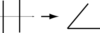
Figure 4.1: Eq. (4.7) maps a strip in the $(y,z)$ plane to a wedge in the $(Y,Z)$ plane

Notice that (4.8) is the metric derived by Polchinski and Witten [8] in the supersymmetric case, but for one notable difference: here the $Y$ direction is not compact. On the other hand, in the new coordinate system $(Y,Z)$ the periodicity under $y\to y+2\pi R$ reflects itself in the orbifold identification

$$Z+i\,Y\ \to\ e^{2\pi i\lambda R}\ (Z+i\,Y)\ ,$$ (4.9)

a two-dimensional rotation ${\cal R}_{\theta}$ in the $(Y,Z)$ plane by an angle $\theta=2\pi\lambda R$. In addition, the orientifold identification $y\rightarrow-y$ maps into a parity $\Pi_{Y}$ times a rotation ${\cal R}_{2\omega}$ by an angle $2\omega$, so that the new $\Omega$ projection is

$$\Omega^{\prime}\ =\ \Omega\ \Pi_{Y}\ {\cal R}_{2\omega}\ ,$$ (4.10)

where $\Omega$ denotes the conventional world-sheet parity. Notice that both the metric and the dilaton in (4.5) depend effectively on the real part of an analytic function, and thus generally on a pair of real variables, aside from the case of [8], where the function is a linear one, so that one of the real variables actually disappears. This simple observation explains the special role of the single-variable solution of [8] in this context.

As sketched in fig. 4.1, the exponential mapping turns the region delimited by the two parallel fixed lines of the orientifold operations in the $(y,z)$ plane into a wedge in the $(Y,Z)$ plane, delimited by the two lines

$$\Omega^{\prime}~{}:\ Y = \tan\omega\ Z\ ,$$

$$\Omega^{\prime}~{}{\cal R}_{2\pi\lambda R}:\ Y = \tan(\pi\lambda R+\omega)\ Z\ ,$$ (4.11)

so that the orientifolds and the branes at $y=0$ form an angle $\theta_{0}=\ \omega$ with the $Z$ axis, while those at $y=\pi R$ form an angle $\theta_{1}=\ \pi\lambda R+\omega$. Notice that the orbifold identification (4.9) implies that in general the two-dimensional $(Y,Z)$ plane contains singularities. In order to avoid subtleties of this type, in what follows we restrict our attention to a case where this complication is absent.

The example we have in mind is a variant of the M-theory breaking model of [20]. Its oriented closed part is related by a T-duality to a Scherk-Schwarz deformation of the toroidally compactified IIB spectrum of [20], described by

$$\mathcal{T} = (|V_{8}|^{2}+|S_{8}|^{2})\Lambda_{m,2n}+(|O_{8}|^{2}+|C_{8}|^{2})\Lambda_{m,2n+1}$$ (4.12)

$$- (V_{8}\bar{S}_{8}+S_{8}\bar{V}_{8})\Lambda_{m+1/2,2n}-(O_{8}\bar{C}_{8}+C_{8}\bar{O}_{8})\Lambda_{m+1/2,2n+1}\ .$$

Here the $\Lambda$’s are toroidal lattice sums, while the orientifold operation is based on $\Omega^{\prime}=\Omega\Pi_{1}$, with $\Pi_{1}$ the inversion along the circle, corresponding to the Klein-bottle amplitude

$$\mathcal{K}\ =\ \frac{1}{2}\,\left\{(V_{8}-S_{8})W_{2n}\ +\ (O_{8}-C_{8})W_{2n+1}\right\}\ ,$$ (4.13)

where the $W$’s are winding sums, and introduces an $O8_{+}$ plane at $y=0$ and an $\overline{O8}_{+}$ plane at $y=\pi R$. For consistency, these demand that no net R-R charge be introduced, a condition met by N pairs of D8-$\overline{D8}$ branes, where the choice $N=16$ is singled out by the connection with M-theory [20]. A simple extension of the arguments in [95] shows that the unoriented closed spectrum described by (4.12) and (4.13) precisely interpolates between the type I string in the $R\rightarrow\infty$ limit and the type 0B orientifold with the tachyonic orientifold projection of [69], to be contrasted with the non-tachyonic $0^{\prime}B$ projection of [73, 74, 75], in the $R\rightarrow 0$ limit.

In order to obtain a classical configuration as in (4.5), without tachyons in the open sector, one can put the $N$ $\overline{D8}$ branes on top of the $O8_{+}$ planes and the $N$ $D8$ branes on top of the $\overline{O8}_{+}$ planes. This configuration differs from the one emphasized in [20] and related to the phenomenon of “brane supersymmetry”, with the $D8$ on top of the $O8_{+}$ and the $\overline{D8}$ on top of the $\overline{O8}_{+}$, by an overall interchange of the positions of branes and anti-branes. This has an important physical effect: whereas in the model of [20] both the NS-NS tadpoles and the R-R charges are locally saturated at the two endpoints, in this case there is a local unbalance of charges and tensions that results in an overall attraction between the endpoints driving the orientifold system toward a vanishing value for the radius $R$.

The resulting open string amplitudes

$$\mathcal{A} = \frac{N^{2}+M^{2}}{2}\ (V_{8}-S_{8})W_{n}+NM(O_{8}-C_{8})W_{n+1/2}\ ,$$

$$\mathcal{M} = -\frac{N+M}{2}\ \hat{V}_{8}W_{n}-\frac{N+M}{2}\hat{S}_{8}(-1)^{n}W_{n}\ ,$$ (4.14)

describe matter charged with respect to an $SO(N)\times SO(M)$ gauge group, where $N=M$ on account of the R-R tadpole conditions, with nine-dimensional massless Majorana fermions in the symmetric representations ($N(N+1)/2$,1) and (1,$M(M+1)/2$) and massive fermions in the bi-fundamental representation ($N,M$). Notice that tachyons appear for small values of $R$. This spectrum should be contrasted with the one of [20] exhibiting “brane supersymmetry”, where the massless fermions are in antisymmetric representations. It is a simple exercise to evaluate tensions and R-R charges at the two ends of the interval:

$$T_{0}\ =\ (N-16)T_{8}\ ,\qquad T_{1}\ =\ (N-16)T_{8}\ ,$$

$$q_{0}\ =\ -\,(N+16)T_{8}\ ,\qquad q_{1}\ =\ (N+16)T_{8}\ .$$ (4.15)

These translate into corresponding values for the parameters $\lambda$ and $\omega$ of the classical solution in (4.4), that in this case are

$$\lambda=\frac{1}{R}\ ,\quad\cos\omega=\frac{16-N}{16+N}\ .$$ (4.16)

Hence, in the new coordinate system (4.6) the orbifold operation (4.9) becomes a $2\pi$ rotation, and can thus be related to the fermion parity $(-1)^{F}$, while the orientifold operation $\Omega^{\prime}$ combines a world-sheet parity with a rotation. Notice also that $\lambda\pi R=\pi$, and therefore the $O_{+}$ and $\overline{O}_{+}$ planes are actually juxtaposed in the $(Y,Z)$ plane along the real axis $Y=0$, forming somehow a bound state with vanishing total R-R charge. To be precise, the $O_{+}$ plane lies along the half-line $Y=0,$ $Z>0,$ while the ${\bar{O}}_{+}$ plane lies along the complementary half-line $Y=0,$ $Z<0.$ The end result is that in the $(Y,Z)$ plane one is describing the $0B$ (or $IIB/(-1)^{F}$) string, subject to the orientifold projection $\Omega^{\prime}=\Omega\Pi_{Y}$, where $Y,$ as already stressed, is here a noncompact coordinate. By our previous arguments, all this is somehow equivalent to the type IIB orientifold compactified on a circle that we started with. In more physical terms, the attraction between the sets of $D(\overline{D})$ branes and $O(\overline{O})$ planes at the ends of the interval drives them to collapse into suitable systems of $D$-branes and $O$-planes carrying no net R-R charge, that should be captured by the static solutions of the effective action (4.1), and these suggest a relation to the $0B$ theory. In this respect, a potentially singular fate of space time opens the way to a sensible string vacuum. We would like to stress, however, that the picture supplied by the classical solution (4.5) is incomplete, since the origin $Y=Z=0$ is actually the site of a singularity. Indeed, the resulting $O$-plane system has no global R-R charge, but has nonetheless a dipole structure: its $Z<0$ portion carries a positive charge, while its $Z>0$ portion carries a negative charge. While we are not able to provide more stringent arguments, it is reasonable to expect that the condensation of the open and closed-string tachyons emerging in the $R\to 0$ limit can drive a natural redistribution of the dipole charges between the two sides, with the end result of turning the juxtaposed $O$ and $\overline{O}$ into a charge-free type-$O$ orientifold plane. If this were the case, not only the resulting geometry of the bulk, but also the $D/O$ systems, would become those of the $0B$ string.

In order to provide further evidence for this, let us look more closely at the type 0B orientifold we identified, using the original ten-dimensional construction of [69]. The 0B torus amplitude is [68]

$$\mathcal{T} = (|O_{8}|^{2}+|V_{8}|^{2}+|S_{8}|^{2}+|C_{8}|^{2})\ ,$$ (4.17)

while the orientifold operation includes the parity $\Omega^{\prime}=\Omega\Pi_{Y}$, so that the Klein-bottle amplitude

$$\mathcal{K}=\frac{1}{2}\ \left(O_{8}+V_{8}-S_{8}-C_{8}\right)\$$ (4.18)

introduces an $O8$ plane at $Y=0$, without R-R charge and with a tension that precisely matches that of the type-IIB $O8$-$\overline{O8}$ bound state. In general the type-0 orientifold planes, being bound states of IIB orientifold planes, have in fact twice their tension. In the present case, the parity $\Pi_{Y}$ along a noncompact coordinate sends one of the orientifold planes to infinity, with the net result of halving the total tension seen in the $(Y,Z)$ plane.

One can also add to this system two different types of brane-antibrane pairs, and the open-string amplitudes read [69]

$$\mathcal{A} = \frac{n_{o}^{2}+n_{v}^{2}+n_{s}^{2}+n_{c}^{2}}{2}\ V_{8}+(n_{o}n_{v}+n_{s}n_{c})\ O_{8}$$

$$- (n_{s}n_{v}+n_{c}n_{o})\ S_{8}-(n_{s}n_{o}+n_{c}n_{v})\ C_{8}\ ,$$

$$\mathcal{M} = -\ \frac{n_{v}+n_{o}+n_{s}+n_{c}}{2}\ \hat{V}_{8}\ ,\$$ (4.19)

while the corresponding R-R tadpole conditions are

$$n_{o}\ =\ n_{v}=\ N\ ,\quad n_{s}\ =\ n_{c}=\ M\ .$$ (4.20)

The gauge group of this type-0 orientifold, $SO(N)^{2}\times SO(M)^{2}$, becomes remarkably similar to that of the type-II orientifold we started from, provided only branes of one type are present, together with the corresponding antibranes, a configuration determined setting for instance $M=0$. The resulting spectrum is then purely bosonic, and the precise statement is that, in the $R\rightarrow 0$ limit, the expected endpoint of the collapse, the spectrum of the type-II orientifold should match the purely bosonic spectrum of this type-0 orientifold, as was the case for their closed sectors. Actually, for the geometry of the $D/O$ configurations this was not totally evident, and the same is true for the open spectrum, due to an apparent mismatch in the fermionic content, but we would like to argue again that a proper account of tachyon condensation does justice to the equivalence.

The open-string tachyon $T_{ai}$ of the type-II orientifold is valued in the bi-fundamental, and therefore carries a pair of indices in the fundamental of the $SO(N)\times SO(N)$ gauge group. In the $R\rightarrow 0$ limit, all its Kaluza-Klein excitations acquire a negative mass squared. These tachyons will naturally condense, with $<T_{ai}>=T(y)\ \delta_{ai}$, where $T(y)$ denotes the tachyonic kink profile, breaking the gauge group to its diagonal $SO(N)$ subgroup, so that, after symmetry breaking and level by level, the fermions will fall in the representations

$$C^{(k+1/2)}~{}:\frac{N(N-1)}{2}+\frac{N(N+1)}{2}\ ,$$

$$S^{(2k)}~{}:\frac{N(N+1)}{2}\ ,\qquad S^{(2k+1)}~{}:\frac{N(N-1)}{2}\ .$$ (4.21)

In the $R\rightarrow 0$ limit the appropriate description of tachyon condensation is in the T-dual picture, and after a T-duality the interactions within the open sector must respect Kaluza-Klein number conservation. Therefore the Yukawa interactions, that before symmetry breaking are of the type

$$S_{(ij)}^{(2k)}C_{ja}^{t,(k+1/2)}T_{ai}^{(k-1/2)}\ ,\qquad S_{(ab)}^{(2k)}C_{bi}^{(k+1/2)}T_{ia}^{t,(k-1/2)}\ ,$$

$$S_{[ij]}^{(2k+1)}C_{ja}^{t,(k+1/2)}T_{ai}^{(k+1/2)}\ ,\qquad S_{[ab]}^{(2k+1)}C_{bi}^{(k+1/2)}T_{ia}^{t,(k+1/2)}\ ,$$ (4.22)

will give rise to the mass terms $S_{(ij)}C_{(ji)}$ , $S_{[ij]}C_{[ji]}$. The conclusion is that the final low-lying open spectra are bosonic on both sides and actually match precisely.

A more direct argument for the equivalence we are proposing would follow from a natural extension of Sen’s description of tachyon condensation [96]. As we have already stressed, the $O8$ and $\overline{O8}$ attract one another and drive the orientifold to a collapse. In the T-dual picture, the $O9$ and $\overline{O9}$ condense into a non-BPS orientifold plane in one lower dimension, that in the $R\rightarrow 0$ limit becomes the type-0 orientifold plane that we have described above. This type of phenomenon can plausibly be related to the closed-string tachyon non-trivial profile in this model, in a similar fashion to what happens for the open-string tachyon kink profile in $D$-$\overline{D}$ systems. At the same time, after T-duality the $D9$ and $\overline{D9}$ branes decay into non-BPS $D8$ branes via the appropriate tachyon kink profile. Due to the new $(-1)^{F}$ operation, these new non-BPS type-II branes match directly the non-BPS type-0 branes discussed in [69, 97], since the $(-1)^{F}$ operation removes the unwanted additional fermions. Let us stress that String Theory can resolve in this fashion the potential singularity associated to an apparent collapse of space-time: after tachyon condensation, the $O$-$\overline{O}$ attraction can give birth to a well defined type-0 vacuum.

In this example one is confronted with the ideal situation in which a vacuum redefinition can be analyzed to some extent in String Theory. In general, however, a string treatment in such detail is not possible, and it is therefore worthwhile to take a closer look, on the basis of the intuition gathered from Field Theory, at how the conventional perturbative string setting can be adapted to systems in need of vacuum redefinitions, and especially at what it can teach us about the generic features of the redefinitions. We intend to return to this issue in a future publication [32].

4.2 Threshold corrections in open strings and $NS$-$NS$ tadpoles

While $NS$-$NS$ tadpoles ask for classical resummations that are very difficult to perform systematically, it is often possible to identify physical observables for which resummations are needed only at higher orders of perturbation theory. This happens whenever, in the appropriate limit of moduli space (infinite tube length, in the case of disk tadpoles), massless exchanges cannot be attached to the sources. Examples of quantities of such type are provided by the quantum corrections to gauge couplings, commonly known as threshold corrections [101]. If the tree-level gauge coupling is $1/g^{2}$, the one-loop threshold corrections $\Delta$ are defined as

$$\left.\frac{4\pi^{2}}{g^{2}}\right|_{\rm one-loop}\ =\ \left.\frac{4\pi^{2}}{g^{2}}\right|_{\rm tree-level}\ +\ \Delta(\mu,\Phi_{i})\ ,$$ (4.23)

where $\Delta$ depends on the energy scale $\mu$ and on the moduli $\Phi_{i}$.

The study of quantum corrections to gauge couplings is very important from a phenomenological point of view. From Quantum Field Theory, we know that coupling constants run with energy due to the loop contributions of charged particles. Therefore, it is necessary to take into account the radiative corrections predicted by String Theory, in order to achieve a more realistic matching with the low-energy world, and indeed the study of threshold corrections is closely related to the issue of unification in supersymmetric theories. Moreover, as we said, threshold corrections depend on the moduli of the model in consideration, and the knowledge of this dependence is important for the issue of moduli stabilization after supersymmetry breaking.

Let us now discuss some properties of threshold corrections. From string computations one can see that $\Delta$ has the following general structure

$$\Delta\ =\ \frac{1}{4}\int_{0}^{\infty}\frac{dt}{t}{\cal B}(t)\ .$$ (4.24)

This integral is typically divergent in the (open) infrared limit, due to the massless charged particles circulating in the loop. Moreover, thinking of the model we want to study as compactified to four dimensions, for $t\to\infty\$ $\Delta$ has to reproduce the correct logarithmic divergence of the four-dimensional low-energy effective field four-dimensional low-energy effective field theory. Therefore we expect that, in such a converge to the usual one-loop $\beta$-function coefficient of the four-dimensional low energy gauge theory under consideration

$$\lim_{t\rightarrow\infty}{\cal B}(t)\ =\ b\ .$$ (4.25)

where $b$ is given by the usual formula

$$b\ =\ -\frac{11}{3}C_{2}(adj)+\frac{2}{3}\sum_{R}T(R)+\frac{1}{3}\sum_{r}T(r)\ ,$$ (4.26)

with $C_{2}(adj)$ the quadratic Casimir of the adjoint representation, and $T(R)$ and $T(r)$ the Dynkin indices of the representation $R$ for the four-dimensional Weyl fermions and of the representation $r$ for the four-dimensional complex scalars .

On the other hand, the (open) ultraviolet limit, corresponding to the infrared $\ell\to\infty$ limit in the transverse closed channel, in all supersymmetric cases is finite since the divergences arising from the propagation of massless closed states going into the vacuum are eliminated by tadpole cancellations.

In this Section we are interested in the ultraviolet limit of one-loop threshold corrections for models with supersymmetry breaking and NS-NS tadpoles. We will consider at first the Sugimoto model compactified on $T^{6}$. Then we will proceed to analyze the orbifold $T^{4}/{\mathbb{Z}}_{2}\times T^{2}$, both in the case of brane supersymmetry breaking and in the supersymmetric case, but with the addition of a brane-antibrane system that breaks supersymmetry. Finally, we will analyze the $0^{\prime}B$ model compactified on a torus $T^{6}$. In all these models, that have parallel branes and are free of closed tachyons, we will show that the one-loop threshold corrections are ultraviolet finite, despite the presence of uncancelled NS-NS tadpoles. One can understand this finiteness noting that in the $l\rightarrow\infty$ limit the string amplitudes acquire a field-theory interpretation in terms of dilaton and graviton exchanges between $Dp$-branes and $Op$-planes. For parallel localized sources, the relevant terms in the effective Lagrangian are

$$S = \frac{1}{2k_{10}^{2}}\int d^{10}x\sqrt{-G}\biggl{\{}R-\frac{1}{2}(\partial\varphi)^{2}-\frac{1}{2(p+2)~{}!}e^{(5-p-2)\varphi/2}F_{p+2}^{2}\biggr{\}}$$ (4.27)

$$- \int_{{\bf y}={\bf y_{i}}}d^{p+1}\xi\biggl{\{}\sqrt{-\gamma}\left[T_{p}e^{(p-3)\varphi/4}+e^{(p-7)\varphi/4}{\rm tr\,}F_{\mu\nu}^{2}\right]+qC^{(p+1)}\biggr{\}}\ ,$$

where ${\bf\xi}$ are brane world-volume coordinates, $q=\pm 1$ distinguishes between branes or $O$-planes and antibranes or $\overline{O}$-planes, $G$ is the 10-dimensional metric, $\gamma$ is the induced metric and $C^{(p+1)}$ denotes a $R$-$R$ form that couples to the branes. The result for the one-loop corrections to gauge couplings, obtained using (4.27) while treating for simplicity the K-K momenta as a continuum, is proportional to

$$T_{p}\int\frac{d^{9-p}k}{(2\pi)^{9-p}}\biggl{\{}-T^{\mu\nu}\,\langle h_{\mu\nu}h_{\rho\sigma}\rangle\,\eta^{\rho\sigma}\ +\ {\rm tr\,}F^{2}\langle\,\varphi\varphi\rangle\,\frac{(p-3)(p-7)}{16}\biggr{\}}\ ,$$ (4.28)

where

$$\langle h_{\mu\nu}h_{\rho\sigma}\rangle\ =\ \frac{1}{2k^{2}}\left(\eta_{\mu\rho}\eta_{\nu\sigma}+\eta_{\mu\sigma}\eta_{\nu\rho}-\frac{1}{4}\eta_{\mu\nu}\eta_{\rho\sigma}\right)$$ (4.29)

is the ten-dimensional graviton propagator in De Donder gauge,

$$\langle\varphi\varphi\rangle\ =\ \frac{1}{k^{2}}$$ (4.30)

is the ten-dimensional dilaton propagator, and

$$T_{\mu\nu}={\rm tr\,}\left(F_{\mu\rho}F_{\nu}^{\rho}-\frac{1}{4}\eta_{\mu\nu}F^{2}\right)$$ (4.31)

is the vector energy-momentum tensor.

The nice thing to notice in (4.28) is that the dilaton and graviton exchanges cancel precisely, source by source, in the threshold corrections, ensuring that the result is actually finite in spite of the presence of the dilaton and graviton tadpoles. This fact could be explained considering that in models with parallel branes with supersymmetry broken on the branes, the bulk is supersymmetric and therefore, in the (closed) infrared limit, threshold corrections are essentially given by supersymmetric expressions. actually, this type of argument applies also the non-tachyonic type $0^{\prime}B$ orientifold.

4.2.1 Background field method

The main goal of this Section is the computation of the one-loop corrections to gauge couplings in a number of string models with supersymmetry breaking. We will focus our attention on the ultraviolet behavior of such quantities, showing their UV finiteness in spite of the emergence of NS-NS tadpoles. Here, we review the background field method [102], the tool we shall use to extract from the one-loop open partition functions the expressions for threshold corrections.

The starting point is the one-loop vacuum energy that (in the Euclidean case) is provided by (1.41)

$$\Gamma\ =\ -\frac{V}{2}\int_{\epsilon}^{\infty}\frac{dt}{t}\ \int\frac{d^{D}p}{(2\pi)^{D}}\ e^{-tp^{2}}\ \mathrm{Str}\left(e^{-tM^{2}}\right)\ ,$$ (4.32)

We now restrict the previous formula to the case of open strings for which $M^{2}=\frac{1}{\alpha^{\prime}}(N+a)$. Performing the integral over momenta

$$\int\frac{dp^{D}}{(2\pi)^{D}}\ e^{-tp^{2}}\ =\ \frac{1}{(4\pi t)^{\frac{D}{2}}}\ ,$$ (4.33)

after a rescaling of the integration variable, $t=\alpha^{\prime}\pi\tau$, we obtain the general form of the annulus amplitude

$$\Gamma\ =\ -\frac{V_{D}}{2(4\alpha^{\prime}\pi^{2})^{\frac{D}{2}}}\ \int_{0}^{\infty}\frac{d\tau}{\tau^{\frac{D}{2}+1}}\ \mathrm{Str}\ e^{-\pi\tau\ (N+a)}\ .$$ (4.34)

The four-dimensional case is then recovered compactifying six dimensions on a torus, for example. Thus, let us fix $D=4$ and add the sum over internal momenta

$$P\ =\ \sum_{m}e^{-\alpha^{\prime}\pi\tau\ m^{\rm T}g^{-1}m}\ .$$ (4.35)

Of course, we have to add also the Möbius contribution, that as usual is obtained from the annulus amplitude projecting it with the orientifold operation $P=(1+\epsilon\Omega)/2$, where $\Omega$ is the world-sheet parity, while $\epsilon$ is a sign. Putting the factor $1/2$ of the orientifold projection inside the definition of $\cal{A}$ and $\cal{M}$, and considering the energy per unit volume, the general amplitudes for the unoriented open sector are given by

$$\cal{A}\ = \ -\frac{1}{(8\alpha^{\prime}\pi^{2})^{2}}\ \int_{0}^{\infty}\frac{d\tau}{\tau^{3}}\ \mathrm{Str}\ e^{-\pi\tau\ (N+a)}\ P\ ,$$

$$\cal{M}\ = \ -\frac{1}{(8\alpha^{\prime}\pi^{2})^{2}}\ \int_{0}^{\infty}\frac{d\tau}{\tau^{3}}\ \mathrm{Str}\ \left(e^{-\pi\tau(N+a)}\ \epsilon\Omega\ \right)\ P\ .$$ (4.36)

We now turn on a background magnetic field, for example in the $X^{1}$ direction

$$F_{23}\ =\ BQ\ ,$$ (4.37)

where $X^{0}\ldots X^{3}$ are the uncompactified dimensions and $Q$ is a generator of the gauge group, chosen with a suitable normalization . The net effect of the magnetic field on the open amplitudes [83] is to shift the oscillator frequencies of the complex coordinate $X_{2}+iX_{3}$ by an amount $\epsilon$, where

$$\pi\epsilon\ =\ \tan^{-1}(\pi q_{a}B)+\tan^{-1}(\pi q_{b}B)\ ,$$ (4.38)

and $q_{a(b)}$ are the eigenvalues of the generator $Q$ acting on the Chan-Paton charges at the left (right) endpoints of the string. Moreover, we fixed $2\alpha^{\prime}=1$, and we will use this convention in all the following computations.
The partition functions in the presence of $B$ are simply obtained replacing

$$p^{\mu}p_{\mu}\qquad{\rm with}\qquad-(p_{0})^{2}\ +\ (p_{1})^{2}\ +(2n+1)\epsilon\ +\ 2\epsilon\ \Sigma_{23}$$ (4.39)

and

$$(\sum_{bos}-\sum_{ferm})\ \int\frac{d^{4}p}{(2\pi)^{4}}\qquad{\rm with}\qquad(\sum_{bos}-\sum_{ferm})\frac{(q_{a}+q_{b})B}{2\pi}\ \sum_{n=0}\int\frac{d^{2}p}{(2\pi)^{2}}\ ,$$ (4.40)

where $n$ labels the Landau levels, $(q_{a}+q_{b})B/2\pi$ is the degeneracy of Landau levels per unit area, and $\Sigma$ is the spin along the direction of the magnetic field. Threshold corrections at one-loop are then obtained expanding the total one-loop vacuum energy in terms of $B$ [102]

$$\Lambda(B)\ =\left({\cal T}+{\cal K}+{\cal A}(B)+{\cal M}(B)\right)\ =\ \Lambda_{0}+\frac{1}{2}\left(\frac{B}{2\pi}\right)^{2}\Lambda_{2}+o(B^{4})\ ,$$ (4.41)

where the closed sector does not contribute to the expansion, since one can charge only the ends of open strings. The first term, $\Lambda_{0}$, is the one-loop cosmological constant and vanishes for a supersymmetric theory, while the quadratic term in the background field, $\Lambda_{2}$, gives just the one-loop threshold corrections to gauge couplings.

4.2.2 Sugimoto model

Let us consider the Sugimoto model compactified on $T^{6}$. We recall that the gauge group is $USp(32)$ and that the model contains $N$ $\overline{{\rm D}9}$ branes and an O9_- plane and thus the NS-NS tadpole is not cancelled. The starting point to compute the threshold corrections is to write the open amplitudes. First of all we consider the case $B=0$. The annulus and Möbius amplitudes, with their normalization and the integral and the contributions of the internal bosons explicitly displayed, are (see eq. (1.109) with $n_{+}=0\$, $\ n_{-}=N=32\$, $\ \epsilon_{NS}=\epsilon_{R}=+1$)

$${\cal A} = -\frac{N^{2}}{(4\pi^{2})^{2}}\int\frac{d\tau}{\tau^{3}}\ \frac{(V_{8}-S_{8})}{\eta^{8}}\ P^{(6)}\ ,$$

$${\cal M} = -\frac{N}{(4\pi^{2})^{2}}\int\frac{d\tau}{\tau^{3}}\ \frac{(\hat{V}_{8}+\hat{S}_{8})}{\hat{\eta}^{8}}\ P^{(6)}\ ,$$ (4.42)

where $P^{(6)}$ is defined as in (4.35). The integration moduli, $i\tau/2$ for the annulus amplitude and $i\tau/2+1/2$ for the Möbius strip, are understood. Expressing the $so(8)$ characters in terms of $\vartheta$-functions (1.3), the amplitudes read

$${\cal A} = -\ \frac{N^{2}}{2(4\pi^{2})^{2}}\int\frac{d\tau}{\tau^{3}}\ \sum_{\alpha,\beta}\eta_{\alpha\beta}\ \frac{\vartheta^{4}\left[{\textstyle{\alpha\atop\beta}}\right]}{\eta^{12}}\ P^{(6)}\ ,$$

$${\cal M} = -\ \frac{N}{2(4\pi^{2})^{2}}\int\frac{d\tau}{\tau^{3}}\ \sum_{\alpha,\beta}\eta_{\alpha\beta}\ e^{2\pi i\alpha}\ \frac{\vartheta^{4}\left[{\textstyle{\alpha\atop\beta}}\right]}{\eta^{12}}\ P^{(6)}\ ,$$ (4.43)

where $\alpha$ and $\beta$ are $0,1/2$, and $\eta_{\alpha\beta}=(-)^{2\alpha+2\beta+4\alpha\beta}$. In Appendix A we recall the definition of the Jacobi $\vartheta$-functions and some of their properties.

At this point we turn on a background magnetic field, $F_{23}=QB$, where $Q$ is a $U(1)$ generator in the Cartan subalgebra of the gauge group $USp(32)$. The magnetic filed shifts the frequency of string oscillators by

$$\pi\epsilon=\left\{\begin{array}[]{ll}\tan^{-1}{(\pi q_{a}B)}+\tan^{-1}{(\pi q_{b}B)}\ \simeq\ \pi(q_{a}+q_{b})B-\frac{\pi^{3}}{3}(q_{a}^{3}+q_{b}^{3})B^{3}\ ,&\quad{\cal A}\\ &\\ 2\tan^{-1}{\pi q_{a}B}\ \simeq\ 2\pi q_{a}B-\frac{2\pi^{3}}{3}q_{a}^{3}B^{3}\ .&\quad{\cal M}\end{array}\right.$$ (4.44)

In practice, if the magnetic field acts only on two coordinates, in our case $X^{2}$ and $X^{3}$, one has to perform the replacement

$$\frac{\vartheta\left[{\textstyle{\alpha\atop\beta}}\right](0|\tau)}{\eta}\ \longrightarrow\frac{\vartheta\left[{\textstyle{\alpha\atop\beta}}\right]\left(i\epsilon\tau/2|\tau\right)}{\eta}\ ,$$ (4.45)

for the two fermionic degrees of freedom affected by $B$, and

$$\frac{1}{\eta^{2}}\ \longrightarrow\frac{\eta}{\vartheta_{1}(i\epsilon\tau/2)}\ ,$$ (4.46)

for the bosonic coordinates. Then the amplitudes in the presence of $B$ read

$${\cal A} = -\ \frac{i\pi B}{2(4\pi^{2})^{2}}\int\frac{d\tau}{\tau^{2}}\ \sum_{a,b=1}^{32}(q_{a}+q_{b})\ \sum_{\alpha,\beta}\eta_{\alpha\beta}\ \frac{\vartheta\left[{\textstyle{\alpha\atop\beta}}\right]\left(\frac{i\epsilon\tau}{2}\right)}{\vartheta_{1}\left(\frac{i\epsilon\tau}{2}\right)}\ \frac{\vartheta^{3}\left[{\textstyle{\alpha\atop\beta}}\right]}{\eta^{9}}\ P^{(6)}\ ,$$

$${\cal M} = -\ \frac{i\pi B}{(4\pi^{2})^{2}}\int\frac{d\tau}{\tau^{2}}\ \sum_{a=1}^{32}q_{a}\ \sum_{\alpha,\beta}\eta_{\alpha\beta}\ e^{2\pi i\alpha}\ \frac{\vartheta\left[{\textstyle{\alpha\atop\beta}}\right]\left(\frac{i\epsilon\tau}{2}\right)}{\vartheta_{1}\left(\frac{i\epsilon\tau}{2}\right)}\ \frac{\vartheta^{3}\left[{\textstyle{\alpha\atop\beta}}\right]}{\eta^{9}}\ P^{(6)}\ ,$$ (4.47)

and one can verify that in the small magnetic field limit these expressions reduce to the ones in (4.2.2).

Since we are interested in the open ultraviolet limit, it is convenient to pass in the transverse channel where such a limit corresponds to the infrared $\ell\rightarrow\infty$ limit. For the annulus amplitude the transformation is $t=\tau/2$ and then $S:t\rightarrow 1/\ell$. We get a factor $2^{-3}$ from the lattice sum and a factor $2^{-1}$ from the integral measure, that together with the factor $1/2$ from the normalization of ${\cal A}$ reconstruct the right power $2^{-5}$. For the Möbius strip one has to perform a $P$-modular transformation, $i\tau/2+1/2\rightarrow i/2t+1/2$ and then make the substitution $\ell=t/2$. From the measure we gain a factor $2$, and defining

$$W^{(6)}\ =\ \sum_{n}\ e^{-\pi\ell\ n^{\rm T}gn/2\alpha^{\prime}}\ ,$$ (4.48)

and

$$v^{(d)}\ =\ \sqrt{\frac{{\rm det}\ g}{\alpha^{\prime\ d}}}\ ,$$ (4.49)

the amplitudes in the transverse channel are given by

$$\tilde{{\cal A}} = -\ \frac{\pi B\ v^{(6)}2^{-5}}{(4\pi^{2})^{2}}\int d\ell\ \sum_{a,b=1}^{32}(q_{a}+q_{b})\ \sum_{\alpha,\beta}\eta_{\alpha\beta}\ \frac{\vartheta\left[{\textstyle{\alpha\atop\beta}}\right](\epsilon)}{\vartheta_{1}(\epsilon)}\ \frac{\vartheta^{3}\left[{\textstyle{\alpha\atop\beta}}\right]}{\eta^{9}}\ W^{(6)}\ ,$$

$$\tilde{{\cal M}} = -\ \frac{2\pi Bv^{(6)}}{(4\pi^{2})^{2}}\int d\ell\ \sum_{a=1}^{32}q_{a}\ \sum_{\alpha,\beta}\eta_{\alpha\beta}\ e^{2\pi i\alpha}\ \frac{\vartheta\left[{\textstyle{\alpha\atop\beta}}\right]\left(\frac{\epsilon}{2}\right)}{\vartheta_{1}\left(\frac{\epsilon}{2}\right)}\ \frac{\vartheta^{3}\left[{\textstyle{\alpha\atop\beta}}\right]}{\eta^{9}}\ W^{(6)}_{e}\ ,$$ (4.50)

where the integrands are computed for $\tau=i\ell$ for the annulus and for $\tau=i\ell+1/2$ for the Möbius, and where as usual in the transverse Möbius only even windings propagate. Moreover, we used the fact that $\vartheta_{2,3,4}(z)$ are even functions of $z$, while $\vartheta_{1}(z)$ is odd. At this point one can use the identity (A.13)

$$\vartheta_{3}(z)\vartheta_{3}^{3}-\vartheta_{4}(z)\vartheta_{4}^{3}-\vartheta_{2}(z)\vartheta_{2}^{3}\ =\ 2\vartheta_{1}^{4}(z/2)\ ,$$ (4.51)

obtaining for the transverse amplitudes

$$\tilde{{\cal A}} = -\ \frac{2\pi B\ v^{(6)}2^{-5}}{(4\pi^{2})^{2}}\int d\ell\ \sum_{a,b=1}^{32}(q_{a}+q_{b})\ \frac{\vartheta_{1}^{4}(\epsilon/2)}{\vartheta_{1}(\epsilon)\eta^{9}}\ W^{(6)}\ ,$$

$$\tilde{{\cal M}} = -\ \frac{4\pi Bv^{(6)}}{(4\pi^{2})^{2}}\int d\ell\ \sum_{a=1}^{32}q_{a}\ \frac{\vartheta_{2}(\epsilon/2)\vartheta_{2}^{3}+\vartheta_{1}^{4}(\epsilon/4)}{\vartheta_{1}(\epsilon/2)\eta^{9}}\ W^{(6)}_{e}\ .$$ (4.52)

The contribution proportional to $\vartheta_{1}^{4}$ is what one would obtain in the supersymmetric case from the character $V_{8}-S_{8}$. Since $\mathcal{N}=1$ in $D=10$ corresponds to $\mathcal{N}=4$ in $D=4$, one expects no threshold corrections from such a term. And in fact, since for small $B$

$$\vartheta_{1}(z)\ \simeq\ 2\pi z\eta^{3}\ ,$$ (4.53)

the term proportional to $\vartheta_{1}^{4}$ in the annulus and in the Möbius amplitudes starts at the quartic order in $B$, giving no corrections to gauge coupling. On the other hand, the $\vartheta_{2}$ term in the Möbius strip contributes to threshold corrections. Expanding the $\vartheta$-functions for a small magnetic field

$$\vartheta_{2}(\epsilon/2)\ \simeq\ \vartheta_{2}+\frac{\epsilon^{2}}{8}\vartheta_{2}^{\prime\prime}\ ,$$

$$\vartheta_{1}(\epsilon/2)\ \simeq\ \frac{\epsilon}{2}\vartheta_{1}^{\prime}+\frac{\epsilon^{3}}{48}\vartheta_{1}^{\prime\prime\prime}\ =\ \pi\epsilon\ \eta^{3}+\frac{\epsilon^{3}}{48}\vartheta_{1}^{\prime\prime\prime}\ ,$$ (4.54)

and recalling that for the Möbius amplitude

$$\pi\epsilon\ \simeq\ 2\pi Bq_{a}-\frac{2\pi^{3}}{3}q_{a}^{3}B^{3}\ ,$$ (4.55)

we obtain at the second order in the magnetic field

$$\tilde{\cal M} = -\ \frac{2v^{(6)}}{(4\pi^{2})^{2}}\ N\ \int d\ell\frac{\vartheta_{2}^{4}}{\eta^{12}}\ W^{(6)}_{e}$$ (4.56)

$$-\frac{v^{(6)}B^{2}\ {\rm tr}Q^{2}}{(4\pi^{2})^{2}}\int d\ell\ \frac{\vartheta_{2}^{4}}{\eta^{12}}\ \left(\frac{2\pi^{2}}{3}+\frac{\vartheta_{2}^{\prime\prime}}{\vartheta_{2}}-\frac{\vartheta_{1}^{\prime\prime\prime}}{6\pi\eta^{3}}\right)W^{(6)}_{e}+o(B^{4})\ ,$$

where $N=32$ and ${\rm tr}Q^{2}=\sum_{a=1}^{32}q_{a}^{2}$, where the zeroth order is the contribution due to the uncancelled NS-NS tadpole.

Finally, from the second order terms one extracts the one-loop threshold corrections to the gauge coupling, that is

$$\Lambda_{2}\ =\ -\ \frac{v^{(6)}\ {\rm tr}Q^{2}}{2\pi^{2}}\int d\ell\ \frac{\vartheta_{2}^{4}}{\eta^{12}}\ \left(\frac{2\pi^{2}}{3}+\frac{\vartheta_{2}^{\prime\prime}}{\vartheta_{2}}-\frac{\vartheta_{1}^{\prime\prime\prime}}{6\pi\eta^{3}}\right)W^{(6)}_{e}\ .$$ (4.57)

The good infrared behavior of the last expression can be checked considering that the term proportional to $\vartheta_{2}(\epsilon/2)\vartheta_{2}^{3}$ in the expression for the Möbius transverse amplitude (4.2.2) is independent of $B$ in the $\ell\rightarrow\infty$ limit

$$\lim_{\ell\rightarrow\infty}\pi q_{a}B\ \frac{\vartheta_{2}(\epsilon/2)\ \vartheta_{2}^{3}}{\vartheta_{1}(\epsilon/2)\ \eta^{9}}\ =\ \frac{8\pi q_{a}B}{\tan{(\pi\epsilon/2)}}\ =\ 8,$$ (4.58)

where in the last equality we used the expression for $\epsilon$ given in (4.44).

One can also check that the open infrared limit of threshold corrections reconstruct just the right one-loop $\beta$-function coefficient of the low-energy effective field theory corresponding to the model. To study the behavior of (4.57) in such a limit it is convenient to consider the open channel. Threshold corrections from the open channel come only from the Möbius strip since the annulus is the same as in the supersymmetric theory, and in particular from a term

$$\frac{-i\pi B}{(4\pi^{2})^{2}}\ \int\frac{d\tau}{\tau^{2}}\ \sum_{a=1}^{32}q_{a}\ \frac{2\vartheta_{2}(i\epsilon\tau/2)\vartheta_{2}^{3}}{\vartheta_{1}(i\epsilon\tau/2)\eta^{9}}\ P^{(6)}\ ,$$ (4.59)

that in the $\tau\to\infty$ limit and to the second order in the magnetic field behaves as

$$-\ \frac{1}{3\pi^{2}}B^{2}{\rm tr}Q^{2}\ \int\frac{d\tau}{\tau}\ +\ {\rm IR\ finite\ terms}\ .$$ (4.60)

Hence, the leading open infrared limit of the threshold corrections, with the normalization ${\rm tr_{fund}}Q^{2}=1/2$ of the generator $Q$ in the fundamental representation, are given by

$$\Lambda_{2}=\frac{1}{4}\ \left(-\frac{16}{3}\right)\ \int\frac{d\tau}{\tau}\ ,$$ (4.61)

where $b=-16/3$ should be the one-loop $\beta$-function coefficient given by the usual four-dimensional formula 4.26. In our case the model at the massless field theory level contains a four-dimensional gauge vector together with 3 complex scalars in the adjoint representation and 4 four-dimensional Weyl fermions in the antisymmetric representation, and thus one recovers

$$b=\ -\frac{11}{3}\times 17+\frac{2}{3}\times 4\times 15+\frac{1}{3}\times 3\times 17=-\frac{16}{3}\ ,$$ (4.62)

where for $USp(N)$, with the normalization chosen, $T({\rm fund.})=1/2$, $\ T({\rm adj})=C_{2}({\rm adj})=N/2+1\$ and $T({\rm antisym.})=N/2-1$.

4.2.3 Brane supersymmetry breaking

In this Subsection we will compute the threshold corrections for the $T^{4}/{\mathbb{Z}}_{2}$ brane supersymmetry breaking model [21] compactified on a further $T^{2}$. This model contains D9 branes and $\overline{\rm D5}$ antibranes together with O9₊ and O5_- orientifold planes, and thus the NS-NS tadpoles on the $\overline{\rm D5}$ antibranes are not cancelled. The gauge group is $[SO(16)\times SO(16)]_{9}\times[USp(16)\times USp(16)]_{5}$.

The partition functions, that one can write starting from eqs (2.59) and (2.62) are

$${\cal A} = -\ \frac{1}{2(4\pi^{2})^{2}}\ \int\frac{d\tau}{\tau^{3}}\ \left[(Q_{o}+Q_{v})\left(N^{2}\frac{P^{(4)}}{\eta^{4}}+D^{2}\frac{W^{(4)}}{\eta^{4}}\right)\right.$$

$$\left.+(R_{N}^{2}+R_{D}^{2})(Q_{o}-Q_{v}){\left(\frac{2\eta}{\vartheta_{2}}\right)}^{2}\right.$$

$$\left.+2ND(O_{4}S_{4}-C_{4}O_{4}+V_{4}C_{4}-S_{4}V_{4}){\left(\frac{\eta}{\vartheta_{4}}\right)}^{2}\right.$$

$$\left.+2R_{N}R_{D}(-O_{4}S_{4}-C_{4}O_{4}+V_{4}C_{4}+S_{4}V_{4}){\left(\frac{\eta}{\vartheta_{3}}\right)}^{2}\right]\ \frac{P^{(2)}}{\eta^{2}}\ \frac{1}{\eta^{2}}\ ,$$

$${\cal M} = \frac{1}{2(4\pi^{2})^{2}}\ \int\frac{d\tau}{\tau^{3}}\Biggl{[}N\frac{P^{(4)}}{\hat{\eta}^{4}}(\hat{O}_{4}\hat{V}_{4}+\hat{V}_{4}\hat{O}_{4}-\hat{S}_{4}\hat{S}_{4}-\hat{C}_{4}\hat{C}_{4})$$ (4.63)

$$-D\frac{W^{(4)}}{\hat{\eta}^{4}}(\hat{O}_{4}\hat{V}_{4}+\hat{V}_{4}\hat{O}_{4}+\hat{S}_{4}\hat{S}_{4}+\hat{C}_{4}\hat{C}_{4})$$

$$-N(\hat{O}_{4}\hat{V}_{4}-\hat{V}_{4}\hat{O}_{4}-\hat{S}_{4}\hat{S}_{4}+\hat{C}_{4}\hat{C}_{4})\left({2{\hat{\eta}}\over{\hat{\vartheta}}_{2}}\right)^{2}$$

$$+D(\hat{O}_{4}\hat{V}_{4}-\hat{V}_{4}\hat{O}_{4}+\hat{S}_{4}\hat{S}_{4}-\hat{C}_{4}\hat{C}_{4})\left({2{\hat{\eta}}\over{\hat{\vartheta}}_{2}}\right)^{2}\Biggr{]}\ \frac{P^{(2)}}{\hat{\eta}^{2}}\frac{1}{\hat{\eta}^{2}}\ ,$$

where we wrote explicitly the integrals with their right normalization and the contributions of the two transverse bosons and of the internal bosons. The moduli, $i\tau/2$ for the annulus amplitude, and $i\tau/2+1/2$ for the Möbius strip, are understood. Moreover we recall that

$$N=n_{1}+n_{2}\,,\qquad D=d_{1}+d_{2}\,,$$

$$R_{N}=n_{1}-n_{2}\,,\qquad R_{D}=d_{1}-d_{2}\,,$$ (4.64)

and that

$$N=D=32\ ,\qquad\qquad R_{N}=R_{D}=0\ .$$ (4.65)

The lattice sums $P^{(4)}$ and $W^{(4)}$ on one hand, and $P^{(2)}$ on the other hand, refer respectively to the $T^{4}$ torus of the orbifold compactification and to the additional $T^{2}$ torus.

At this point we magnetize the $\overline{\rm D5}$ antibranes and, as usual, we turn on a magnetic field, $F_{23}=BQ$, along the complex direction $X^{2}+iX^{3}$, where $Q$ corresponds to a $U(1)$ subgroup of one of the two gauge factors $USp(16)$, normalized to ${\rm tr}_{fund}Q^{2}=1/2$. Thinking of such $U(1)$ factor as embedded in $SO(32)$, a good choice for it could be $Q_{32\times 32}={\rm diag}(1/2,-1/2,0\cdots 0)$ if $Q\subset USp(d_{1})\subset SO(32)$, or $Q_{32\times 32}={\rm diag}(0\cdots 0,1/2,-1/2)$ if $Q\subset USp(d_{2})\subset SO(32)$.

Then, since only the $\overline{\rm D5}$ antibranes are magnetized, let us consider only those terms of the amplitudes that can couple to $B$, let us say with an obvious notation ${\cal A}_{\bar{5}\bar{5}+\bar{5}9}$ and ${\cal M}_{\overline{5}}$. Notice that the term proportional to $Q_{o}+Q_{v}$ in the annulus amplitude is the usual supersymmetric combination of $\vartheta$-functions (it is like $V_{8}-S_{8}$)

$${\cal A}^{({\cal N}=4)}\ =\ -\ \frac{1}{4(4\pi^{2})^{2}}\ \int\frac{d\tau}{\tau^{3}}\ D^{2}W^{(4)}P^{(2)}\sum_{\alpha\beta}\eta_{\alpha,\beta}\frac{\vartheta^{4}\left[{\textstyle{\alpha\atop\beta}}\right]}{\eta^{12}}$$ (4.66)

and thus, in the presence of a magnetic field $B$, it would start at the order $B^{4}$, exactly as we already saw in the case of the Sugimoto model. This term in fact would give, after two $T$ dualities along the directions of $T^{2}$ that transform the $\overline{\rm D5}$ antibranes into $\overline{\rm D3}$ antibranes, the threshold corrections to gauge couplings (actually vanishing) of the four-dimensional ${\mathcal{N}}=4$ super Yang-Mills theory.

Using eqs. (1.172) and (2.4) to express the characters in terms of $\vartheta$-functions, the amplitudes read

$${\cal A}_{\bar{5}\bar{5}+\bar{5}9} = {\cal A}^{({\cal N}=4)}\ -\ \frac{1}{4(4\pi^{2})^{2}}\ \int\frac{d\tau}{\tau^{3}}\ \left(4R_{D}^{2}\ \frac{\vartheta_{3}^{2}\ \vartheta_{4}^{2}\ -\ \vartheta_{4}^{2}\ \vartheta_{3}^{2}}{\eta^{6}\ \vartheta_{2}^{2}}\right.$$

$$\left.+\ 2ND\ \frac{\vartheta_{3}^{2}\ \vartheta_{2}^{2}\ -\ \vartheta_{2}^{2}\ \vartheta_{3}^{2}}{\eta^{6}\ \vartheta_{4}^{2}}\right.\left.-2R_{N}R_{D}\ \frac{\vartheta_{4}^{2}\ \vartheta_{2}^{2}\ +\ \vartheta_{2}^{2}\ \vartheta_{4}^{2}}{\eta^{6}\ \vartheta_{3}^{2}}\right)\ P^{(2)}\ ,$$

$${\cal M}_{\bar{5}} = -\ \frac{1}{4(4\pi^{2})^{2}}\ \int\frac{d\tau}{\tau^{3}}\ \Biggl{(}DW^{(4)}P^{(2)}\ \sum_{\alpha\beta}\eta_{\alpha,\beta}\ e^{2\pi i\alpha}\ \frac{\vartheta^{4}\left[{\textstyle{\alpha\atop\beta}}\right]}{\eta^{12}}$$ (4.67)

$$+\ 4DP^{(2)}\ \frac{\vartheta_{3}^{2}\ \vartheta_{4}^{2}\ -\ \vartheta_{4}^{2}\ \vartheta_{3}^{2}}{\eta^{6}\ \vartheta_{2}^{2}}\Biggr{)}\ ,$$

where we used $\vartheta_{1}(0|\tau)=0$ without losing any of the terms that can couple to $B$, since, when we will turn on the magnetic field, in each term containing $\vartheta_{1}$-functions there will be at least one $\vartheta_{1}$ evaluated at $z=0$. Notice that the first contribution to ${\cal M}$, apart from a factor $1/2$ due to the orbifold projection, is the same that we found in the case of Sugimoto model, and so it will contribute to the threshold corrections with the same term we already wrote in eq. (4.57) (apart from the additional factor $1/2$ originating from the orbifold projection).

After the turning on of the magnetic field, whose action on the oscillator frequencies is given by

$$\pi\epsilon=\left\{\begin{array}[]{ll}\tan^{-1}{(\pi q_{a}B)}+\tan^{-1}{(\pi q_{b}B)}\ \simeq\ \pi(q_{a}+q_{b})B-\frac{\pi^{3}}{3}(q_{a}^{3}+q_{b}^{3})B^{3}\ ,&\quad{\cal A}_{{\bar{5}}{\bar{5}}}\\ &\\ \tan^{-1}{(\pi q_{a}B)}\ \simeq\ \pi q_{a}B-\frac{\pi^{3}}{3}q_{a}^{3}B^{3}\ ,&\quad{\cal A}_{\bar{5}9}\\ &\\ 2\tan^{-1}{\pi q_{a}B}\ \simeq\ 2\pi q_{a}B-\frac{2\pi^{3}}{3}q_{a}^{3}B^{3}\ ,&\quad{\cal M}_{\bar{5}}\end{array}\right.\$$ (4.68)

the open amplitudes read

$${\cal A}_{\bar{5}\bar{5}+\bar{5}9}\ =\ {\cal A}^{({\cal N}=4)}(B)$$

$$-\ \frac{i\pi B}{(4\pi^{2})^{2}}\int\frac{d\tau}{\tau^{2}}\ \sum_{a,b=1}^{32}(q_{a}+q_{b})\hat{R}_{aa}\hat{R}_{bb}\ \frac{\vartheta_{3}(i\epsilon\tau/2)\vartheta_{3}\vartheta_{4}^{2}\ -\ \vartheta_{4}(i\epsilon\tau/2)\vartheta_{4}\vartheta_{3}^{2}}{\eta^{3}\ \vartheta_{1}(i\epsilon\tau/2)\vartheta_{2}^{2}}\ P^{(2)}$$

$$-\ \frac{i\pi B16}{(4\pi^{2})^{2}}\int\frac{d\tau}{\tau^{2}}\ \sum_{a=1}^{32}q_{a}\ \frac{\vartheta_{3}(i\epsilon\tau/2)\vartheta_{3}\vartheta_{2}^{2}-\vartheta_{2}(i\epsilon\tau/2)\vartheta_{2}\vartheta_{3}^{2}}{\eta^{3}\ \vartheta_{1}(i\epsilon\tau/2)\vartheta_{4}^{2}}\ P^{(2)}\ ,$$

$${\cal M}_{\bar{5}}\ =\ -\ \frac{i\pi B}{2(4\pi^{2})^{2}}\int\frac{d\tau}{\tau^{2}}\ \sum_{a=1}^{32}q_{a}\ \sum_{\alpha,\beta}\eta_{\alpha\beta}\ e^{2\pi i\alpha}\ \frac{\vartheta\left[{\textstyle{\alpha\atop\beta}}\right]\left(\frac{i\epsilon\tau}{2}\right)}{\vartheta_{1}\left(\frac{i\epsilon\tau}{2}\right)}\ \frac{\vartheta^{3}\left[{\textstyle{\alpha\atop\beta}}\right]}{\eta^{9}}\ W^{(4)}P^{(2)}\$$

$$-\ \frac{2i\pi B}{(4\pi^{2})^{2}}\int\frac{d\tau}{\tau^{2}}\ \sum_{a=1}^{32}q_{a}\ \frac{\vartheta_{3}(i\epsilon\tau/2)\vartheta_{3}\vartheta_{4}^{2}-\vartheta_{4}(i\epsilon\tau/2)\vartheta_{4}\vartheta_{3}^{2}}{\eta^{3}\ \vartheta_{1}(i\epsilon\tau/2)\vartheta_{2}^{2}}\ P^{(2)}\ ,$$ (4.69)

where we used the fact that $R_{N}$ is identically zero and we fixed $N=32$. The matrix $\hat{R}$ is defined as $\hat{R}={\rm diag}(1\cdots 1,-1\cdots-1)$ with $d_{1}=16$ entrances equal to $+1$ and $d_{2}=16$ entrances equal to $-1$.

Now it is easy to perform an $S$-modular transformation for the annulus amplitude, and a $P$ transformation for the Möbius strip, to write the amplitudes in the transverse channel. The annulus gets a factor $1/2$ from the lattice sum and a factor $1/2$ from the integral measure, while the Möbius gets only a factor $2$ from the integral measure. If we denote with $v_{3}$ the normalized (as in 4.49) volume of the further $T^{2}$, and with $v_{1}v_{2}$ the normalized volume of the internal $T^{4}$ (that we think of as $T^{2}\times T^{2}$), the amplitudes in the transverse channel are given by

$$\tilde{\cal A}_{\overline{5}\overline{5}+\overline{5}9} = \tilde{{\cal A}}^{({\cal N}=4)}(B)$$

$$- \frac{\pi Bv_{3}}{4(4\pi^{2})^{2}}\int d\ell\ \sum_{a,b=1}^{32}(q_{a}+q_{b})\hat{R}_{aa}\hat{R}_{bb}\ \frac{\vartheta_{3}(\epsilon)\vartheta_{3}\vartheta_{2}^{2}\ -\ \vartheta_{2}(\epsilon)\vartheta_{2}\vartheta_{3}^{2}}{\eta^{3}\ \vartheta_{1}(\epsilon)\vartheta_{4}^{2}}\ W^{(2)}$$

$$- \frac{4\pi B\ v_{3}}{(4\pi^{2})^{2}}\int d\ell\ \sum_{a=1}^{32}q_{a}\ \frac{\vartheta_{3}(\epsilon)\vartheta_{3}\vartheta_{4}^{2}-\vartheta_{4}(\epsilon)\vartheta_{4}\vartheta_{3}^{2}}{\eta^{3}\ \vartheta_{1}(\epsilon)\vartheta_{2}^{2}}\ W^{(2)}\ ,$$

$$\tilde{\cal M}_{\overline{5}} = -\ \frac{\pi B}{(4\pi^{2})^{2}}\frac{v_{3}}{v_{1}v_{2}}\ \int d\ell\ \sum_{a=1}^{32}q_{a}\ \sum_{\alpha,\beta}\eta_{\alpha\beta}\ e^{2\pi i\alpha}\ \frac{\vartheta\left[{\textstyle{\alpha\atop\beta}}\right]\left(\frac{\epsilon}{2}\right)}{\vartheta_{1}\left(\frac{\epsilon}{2}\right)}\ \frac{\vartheta^{3}\left[{\textstyle{\alpha\atop\beta}}\right]}{\eta^{9}}\ P^{(4)}_{e}W^{(2)}_{e}\$$ (4.70)

$$- \frac{4\pi B\ v_{3}}{(4\pi^{2})^{2}}\int d\ell\ \sum_{a=1}^{32}q_{a}\ \frac{\vartheta_{4}(\epsilon/2)\vartheta_{4}\vartheta_{3}^{2}-\vartheta_{3}(\epsilon/2)\vartheta_{3}\vartheta_{4}^{2}}{\eta^{3}\ \vartheta_{1}(\epsilon/2)\vartheta_{2}^{2}}\ W^{(2)}_{e}\ .$$

At this point we can derive the threshold corrections. Using the definition of $\epsilon$ for ${\cal A}_{\bar{5}\bar{5}}$ given in eq. (4.68), $\epsilon\simeq(q_{a}+q_{b})B$, and recalling that $\vartheta_{2,3,4}(\epsilon)$ are even functions of their arguments, so that in their expansion there is the quadratic term in $\epsilon$ but not the linear one, we can expand the first contribution to the annulus up to second order in the magnetic field, obtaining

$$B\sum_{a,b=1}^{32}(q_{a}+q_{b})\hat{R}_{aa}\hat{R}_{bb}\ \frac{\vartheta_{3}(\epsilon)\vartheta_{3}\vartheta_{2}^{2}\ -\ \vartheta_{2}(\epsilon)\vartheta_{2}\vartheta_{3}^{2}}{\eta^{3}\ \vartheta_{1}(\epsilon)\vartheta_{4}^{2}}\$$

$$\simeq\ {\rm tr}\hat{R}^{2}\ \frac{\vartheta_{3}^{2}\vartheta_{2}^{2}\ -\ \vartheta_{2}^{2}\vartheta_{3}^{2}}{2\pi\eta^{6}\ \vartheta_{4}^{2}}\ +\ \pi B^{2}\sum_{a,b=1}^{32}(q_{a}+q_{b})^{2}\hat{R}_{aa}\hat{R}_{bb}\ ,$$ (4.71)

where we used the identity (A.14) between $\vartheta$-functions

$$\vartheta_{3}^{\prime\prime}\vartheta_{3}\vartheta_{2}^{2}-\vartheta_{2}^{\prime\prime}\vartheta_{2}\vartheta_{3}^{2}\ =\ 4\pi^{2}\eta^{6}\vartheta_{4}^{2}\ .$$ (4.72)

The term proportional to $({\rm tr}\hat{R})^{2}$ is identically zero since $({\rm tr}\hat{R})^{2}=R_{D}^{2}=0$. Also the second term is identically zero, being proportional to $2{\rm tr}(Q^{2}\hat{R})R_{D}+2{\rm tr}(Q\hat{R})^{2}$, and recalling the form of $Q$ and $\hat{R}$. Therefore this part of the annulus gives neither tadpoles nor threshold corrections.

Performing the same type of expansion in the second contribution to the annulus amplitude and in the second contribution to the Möbius amplitude, that have the same structure, it is easy to extract from them the term proportional to $B^{2}$

$$\ \frac{4\pi^{2}B^{2}v_{3}}{(4\pi^{2})^{2}}\ {\rm trQ^{2}}\ \int d\ell\ (W^{(2)}-W^{(2)}_{e})\ ,$$ (4.73)

where we used the suitable definition of $\epsilon$ given in (4.68), and the identity (A.15)

$$\vartheta_{4}^{\prime\prime}\vartheta_{4}\vartheta_{3}^{2}-\vartheta_{3}^{\prime\prime}\vartheta_{3}\vartheta_{4}^{2}\ =\ 4\pi^{2}\eta^{6}\vartheta_{2}^{2}\ .$$ (4.74)

The corresponding contribution to the threshold corrections is then given by

$$\Lambda_{2}^{({\cal N}=2)}\ =\ 2v_{3}\ {\rm tr}Q^{2}\ \int d\ell\ \left(W^{(2)}-W^{(2)}_{e}\right)\ .$$ (4.75)

We have to stress here that this result has the same structure as the four-dimensional ${\cal N}=2$ supersymmetric $T^{4}/{\mathbb{Z}}_{2}\times T^{2}$ model [102], and this fact can be understood if one notes that $ND$ term in the annulus amplitude and the last term in the Möbius amplitude, from which we derived (4.73), are the same as the supersymmetric $T^{4}/{\mathbb{Z}}_{2}$ orbifold, apart from a change of chirality. Moreover we notice that only the short BPS states of ${\cal N}=2$ contributes to $\Lambda_{2}^{({\cal N}=2)}$ while all the string oscillators decouple according to [100, 102]. In order to clarify the relation with ${\cal N}=2$, let us consider the open infrared limit of $\Lambda_{2}^{({\cal N}=2)}$. To do that we come back to the direct channel and we consider the $B^{2}$ terms from the mixed $ND$ sector in the annulus amplitude and from the second addend in the Möbius strip. After using the identities (A.14) and (A.15), we obtain

$$\Lambda_{2}^{({\cal N}=2)}={\rm tr}Q^{2}\ \int\frac{d\tau}{\tau}\left(4P^{(2)}-P^{(2)}\right)\ ,$$ (4.76)

where the first lattice sum comes from the annulus amplitude while the second comes from the Möbius amplitude. The integral can be computed, and indeed this was done in [102], but here let us consider the $\tau\to\infty$ limit after which only the massless Kaluza-Klein recurrences survive. Cutting-off the integration variable to $\tau<1/\mu^{2}$ and fixing ${\rm tr_{fund}}Q^{2}=1/2$, the leading term for $\tau\to\infty$ of $\Lambda_{2}^{({\cal N}=2)}$ is

$$\Lambda_{2}^{({\cal N}=2)}\ =\ -\ \frac{1}{4}\times\frac{1}{2}b^{({\cal N}=2)}\ \ln{\mu^{2}}\ +\ {\rm IR\ finite\ terms}\ ,$$ (4.77)

where

$$b^{({\cal N}=2)}=12\ ,$$ (4.78)

is the standard one-loop $\beta$-function coefficient of the four-dimensional ${\cal N}=2$ super Yang-Mills theory with a gauge multiplet in the adjoint representation of the gauge group $SU(16)$, two hyper-multiplets in the 120, and 16 hyper multiplets in the fundamental representation (this is just the open massless content of the supersymmetric $T^{4}/{\mathbb{Z}}_{2}$ model compactified to four dimensions)

$$b^{({\cal N}=2)}=2\left[-\ C_{2}({\rm adj})\ +\ 2\times T(120)\ +\ 16\times T({\rm fund})\right]=12\ .$$ (4.79)

On the other hand the complete expression for the threshold corrections of this model is obtained adding to $\Lambda_{2}^{({\cal N}=2)}$ the non supersymmetric contribution proportional to $v_{3}/v_{1}v_{2}$ coming from the Möbius strip, whose structure was already analyzed in the case of the Sugimoto model (see eq. (4.2.2)). Taking into account all the contributions, the result is

$$\Lambda_{2} = 2v_{3}\ {\rm tr}Q^{2}\ \int d\ell\ \left(W^{(2)}-W^{(2)}_{e}\right)$$ (4.80)

$$-\ \frac{{\rm tr}Q^{2}}{4\pi^{2}}\ \frac{v_{3}}{v_{1}v_{2}}\ \int d\ell\ \frac{\vartheta_{2}^{4}}{\eta^{12}}\ \left(\frac{2\pi^{2}}{3}+\frac{\vartheta_{2}^{\prime\prime}}{\vartheta_{2}}-\frac{\vartheta_{1}^{\prime\prime\prime}}{6\pi\eta^{3}}\right)P^{(4)}_{e}W^{(2)}_{e}\ .$$

The leading infrared (in the open channel) term is simply obtained adding to $\frac{b^{({\cal N}=2)}}{2}=6$ the non supersymmetric contribution $b^{({\cal N}=0)}=-8/3$ that we already discussed in the case of the Sugimoto model (here there is an additional factor $1/2$ due to the orbifold projection). This sum reproduces the right four-dimensional one-loop $\beta$-function coefficient of the low-energy effective field theory, as one can check using the formula (4.26)

$$b = -\ \frac{11}{3}\times 9\ +\ \frac{4}{3}\times\left(7+16\times\frac{1}{2}\right)\ +\ \frac{2}{3}\times\frac{1}{2}\times 16$$ (4.81)

$$+ \ \frac{1}{3}\times\left(9+2\times\frac{1}{2}\times 16+\frac{1}{2}\times 16\right)=\frac{10}{3}\ ,$$

where the massless four-dimensional fields charged with respect to the magnetic field are: from the $DD$ sector a gauge vector together with a complex scalar in the adjoint representation, 16$\times$2 complex scalars and 16$\times$2 Weyl fermions in the fundamental representation, 2 Weyl fermions in the antisymmetric representation, while from the $ND$ sector 16 complex scalars and 16 Weyl fermions in the fundamental representation.

Summarizing, the resulting threshold corrections (4.80) for the brane supersymmetry breaking model compactified to four dimensions are given by a non supersymmetric term that originates from the Möbius amplitude and by a supersymmetric term to which only the ${\cal N}=2$ BPS states contribute while string oscillators decouple. The remarkable property we want to stress is that, in spite of the presence of NS-NS tadpoles induced by supersymmetry breaking, the threshold corrections are ultraviolet (in the open channel) finite. Moreover, performing two $T$-dualities along the directions of the further torus $T^{2}$, that turn the winding sums $W^{(2)}$ into momentum sums $P^{(2)}$, the volume $v_{3}$ in the T-dual volume $1/v_{3}$ and the $\overline{\rm D5}$ in the $\overline{\rm D3}$, it is easy to see that, in the limit of large internal volume transverse to the $\overline{\rm D3}$, the non supersymmetric contribution is suppressed with respect to the supersymmetric one. Therefore, at the one-loop level, despite the supersymmetry breaking at the string scale on the antibranes, the threshold corrections are essentially determined by the supersymmetric contribution. This result confirms the conjecture, made in [21, 91], that in the brane supersymmetry breaking model (and also in models with brane-antibrane pairs, as we will see in the next Subsection) threshold corrections in codimension larger than two are essentially given by supersymmetric expressions, due to the supersymmetry of the bulk (closed string) spectrum.

4.2.4 Brane-antibrane systems

In this Subsection we compute the threshold corrections for the model obtained adding M D5-$\overline{\rm D5}$ pairs to the usual supersymmetric $T^{4}/Z_{2}$ orbifold of the Type $I$ superstring [69, 67]. Let us begin by recalling the open amplitudes for the supersymmetric model (see (1.196) and (1.201)), that here we write with the integral measure and the bosonic degrees of freedom

$${\cal A} = -\ \frac{1}{2(4\pi^{2})^{2}}\ \int\frac{d\tau}{\tau^{3}}\Biggl{[}\frac{Q_{o}+Q_{v}}{\eta^{8}}\left(N^{2}P^{(4)}_{m}+D^{2}W^{(4)}_{n}\right)$$

$$+\ \left(R_{N}^{2}+R_{D}^{2}\right)\frac{Q_{o}-Q_{v}}{\eta^{4}}\left({2\eta\over\vartheta_{2}}\right)^{2}\ +\ 2ND\,\frac{Q_{s}+Q_{c}}{\eta^{4}}\left({\eta\over\vartheta_{4}}\right)^{2}$$

$$+\ 2R_{N}R_{D}\,\frac{Q_{s}-Q_{c}}{\eta^{4}}\left({\eta\over\vartheta_{3}}\right)^{2}\Biggr{]}\ P^{(2)}_{m},$$

$${\cal M} = \frac{1}{2(4\pi^{2})^{2}}\ \int\frac{d\tau}{\tau^{3}}\left[\frac{\hat{Q}_{o}+\hat{Q}_{v}}{\hat{\eta}^{8}}\left(NP^{(4)}_{m}+DW^{(4)}_{n}\right)\right.$$ (4.82)

$$\qquad\qquad\qquad\quad\qquad\left.-\left(N+D\right)\frac{\hat{Q}_{o}-\hat{Q}_{v}}{\hat{\eta}^{4}}\left({2\hat{\eta}\over\hat{\vartheta}_{2}}\right)^{2}\right]\ P^{(2)}_{m},$$

where

$$N=n+\bar{n}\ ,\qquad D=d+\bar{d}\ ,$$

$$R_{N}=i(n-\bar{n})\ ,\qquad R_{D}=i(d-\bar{d})$$ (4.83)

and $n=\bar{n}=d=\bar{d}=16$. Moreover, we compactified two other dimensions on a further $T^{2}$ torus, as can be seen from the lattice sum $P_{m}^{(2)}$.

Now we add the $M$ brane-antibrane pairs. We denote with $M_{+}=M$ the number of D5 branes and with $M_{-}=M$ the number of $\overline{\rm D5}$ antibranes. Moreover, as in (4.2.4), we parameterize $M_{+}=m_{+}+\overline{m}_{+}$, and $M_{-}=m_{-}+\overline{m}_{-}$, with $m_{\pm}=\bar{m}_{\pm}$ to distinguish branes (or antibranes) from their imagine. If the additional $M_{+}$ D5 branes are placed, together with the original 32, at a given fixed point of the orbifold, while the $M_{-}=M\$ $\overline{\rm D5}$ are placed at a different fixed point, that for simplicity we take to be separated only along one of the internal directions, the resulting gauge group is $U(16)_{9}\times[U(16+m_{+})\times U(m_{-})]_{5}$. The $M$ pairs generate an NS-NS tadpole localized in six dimensions, that would be expected to introduce UV divergences in one-loop threshold corrections.

Let us first analyze the annulus amplitude. The amplitude is obtained changing the RR signs in the transverse channel of the sectors corresponding to exchanges between branes and antibranes, and reads

$${\cal A} = -\ \frac{1}{2(4\pi^{2})^{2}}\ \int\frac{d\tau}{\tau^{3}}\Biggl{[}\frac{Q_{o}+Q_{v}}{\eta^{8}}\left(N^{2}P^{(4)}_{m}+(D+M_{+})^{2}W^{(4)}_{n}+M_{-}^{2}W^{(4)}_{n}\right)$$

$$+\ 2(D+M_{+})M_{-}\ \frac{O_{4}O_{4}+V_{4}V_{4}-S_{4}C_{4}-C_{4}S_{4}}{\eta^{8}}\ W_{n+1/2}^{(4)}$$

$$+\ \left(R_{N}^{2}+R_{D+M_{+}}^{2}+R_{M_{-}}^{2}\right)\ \frac{Q_{o}-Q_{v}}{\eta^{4}}\left({2\eta\over\vartheta_{2}}\right)^{2}$$

$$+\ 2N(D+M_{+})\,\frac{Q_{s}+Q_{c}}{\eta^{4}}\left({\eta\over\vartheta_{4}}\right)^{2}$$

$$+\ 2NM_{-}\ \frac{O_{4}S_{4}-C_{4}O_{4}+V_{4}C_{4}-S_{4}V_{4}}{\eta^{4}}\left({2\eta\over\vartheta_{2}}\right)^{2}$$

$$+\ 2R_{N}R_{D+M_{+}}\,\frac{Q_{s}-Q_{c}}{\eta^{4}}\left({\eta\over\vartheta_{3}}\right)^{2}$$

$$+\ 2R_{N}R_{M_{-}}\ \frac{-O_{4}S_{4}+V_{4}C_{4}+S_{4}V_{4}-C_{4}O_{4}}{\eta^{4}}\ \left({\eta\over\vartheta_{3}}\right)^{2}\Biggr{]}\ P^{(2)}_{m},$$

where the shift of the windings $W_{n+1/2}^{(4)}$ in the term proportional to $(D+M_{+})M_{-}$ is due to the separation between D5 branes and $\overline{D5}$ antibranes. Moreover, we see that there are no mixed terms proportional to $R_{D+M_{+}}R_{M_{-}}$ and the reason is that such a term would come from the one proportional to $W_{n+1/2}^{(4)}$ that has no zero modes to project. The twisted sector is simply the one of the supersymmetric case with $D$ replaced by $D+M_{+}$ and $R_{D}$ by $R_{D+M_{+}}$ together with the addition of mixed terms between the $N\$ D9 branes and the $M_{-}\$ $\overline{D5}$ antibranes, terms that apart from a change of chirality are the same as those of the brane supersymmetry breaking model.

On the other hand, it is easy to write the Möbius amplitude for which the same characters propagate both in the direct and in the transverse channel (see (1.201) and (1.200)), so that in practice one can reverse the signs of the RR sectors proportional to $M_{-}$ directly in the open channel. The amplitude reads

$${\cal M} = \frac{1}{2(4\pi^{2})^{2}}\ \int\frac{d\tau}{\tau^{3}}\left[\frac{\hat{Q}_{o}+\hat{Q}_{v}}{\hat{\eta}^{8}}\left(NP^{(4)}_{m}+(D+M_{+})W^{(4)}_{n}\right)\right.$$ (4.85)

$$\left.+\ M_{-}\ \frac{V_{4}O_{4}+O_{4}V_{4}+C_{4}C_{4}+S_{4}S_{4}}{\hat{\eta}^{8}}\ W_{n}^{(4)}\right.$$

$$-\left.\left(N+D+M_{+}\right)\frac{\hat{Q}_{o}-\hat{Q}_{v}}{\hat{\eta}^{4}}\left({2\hat{\eta}\over\hat{\vartheta}_{2}}\right)^{2}\right.$$

$$\left.-M_{-}\ \frac{V_{4}O_{4}+C_{4}C_{4}-O_{4}V_{4}-S_{4}S_{4}}{\hat{\eta}^{4}}\ \left({2\hat{\eta}\over\hat{\vartheta}_{2}}\right)^{2}\right]\ P^{(2)}_{m}\ .$$

Let us notice that, while the first and third lines in (4.85) are essentially the same as the corresponding terms in the supersymmetric case with $D$ replaced by $D+M_{+}$, the other two lines, proportional to $M_{-}$, describe respectively the interactions of the $\overline{D5}$ antibranes with O5₊ planes, and with an $O9_{+}$ plane. Hence, the fourth line is the same as the corresponding term in the brane supersymmetry breaking model, apart from the usual change of chirality, while the second line has an opposite sign due to the fact that here there is an O5₊ plane while in the brane supersymmetry breaking model there is an O5_- plane.

At this point we can proceed with the background field method. Let us choose a $U(1)$ generator $Q$ in the Cartan subalgebra of the group $SU(16+m_{+})$, with the usual normalization ${\rm tr}_{fund}Q^{2}=1/2$, where the generator $Q$ has no components along the anomalous $U(1)$ factor. Moreover in the Chan-Paton basis in which we wrote the amplitudes (4.85) and (4.2.4) the fundamental and anti-fundamental representations of the group are disentangled [67].

The only sectors that can couple to the magnetic field are the ones proportional to the total number of antibranes $D+M_{+}$. In fact, the terms linear in $R_{N}$ vanish identically since $R_{N}=0$. Moreover, if we denote with $J$ the total number of D5 branes, say $J=D+M_{+}=j+\bar{j}$, and we parameterize $R_{J}=R_{D+M_{+}}$ following $R_{J}=i(j-\bar{j})$, with $j=\bar{j}$, the $R^{2}_{J}$ term in the annulus amplitude is proportional to

$$R_{J}^{2}\ (Q_{0}-Q_{v})\ =\ -(j^{2}+\bar{j}^{2}-2j\bar{j})\ (Q_{o}-Q_{v})\ ,$$ (4.86)

and after the coupling with $B$ it becomes

$$-\biggl{[}\sum_{a,b=1}^{j}(q_{a}+q_{b})\ \hat{R}_{aa}\hat{R}_{bb}+\sum_{\bar{a},\bar{b}=\bar{1}}^{\bar{j}}(\bar{q}_{\bar{a}}+\bar{q}_{\bar{b}})\hat{R}_{\bar{a}\bar{a}}\hat{R}_{\bar{b}\bar{b}}$$

$$-\sum_{a=1}^{j}\sum_{\bar{b}=\bar{1}}^{\bar{j}}(q_{a}+\bar{q}_{\bar{b}})\ \hat{R}_{aa}\hat{R}_{\bar{b}\bar{b}}-\sum_{\bar{a}=\bar{1}}^{\bar{j}}\sum_{b=1}^{j}(\bar{q}_{\bar{a}}+q_{b})\ \hat{R}_{\bar{a}\bar{a}}\hat{R}_{bb}\biggr{]}(Q_{o}-Q_{v})(B),$$ (4.87)

where $q_{a,b}$ and $\bar{q}_{\bar{a},\bar{b}}$ run over the fundamental or the anti-fundamental representations of the unitary gauge group and the matrices $\hat{R}$ are $\hat{R}_{aa}=\hat{R}_{bb}=\mathbf{1}_{j\times j}$ and $\hat{R}_{\bar{a}\bar{a}}=\hat{R}_{\bar{b}\bar{b}}=\mathbf{1}_{\bar{j}\times\bar{j}}$. Moreover, we left implicit the dependence of $Q_{o}-Q_{v}$ on $(q_{a}+q_{b})$. Then, expanding for small magnetic field the character $Q_{o}-Q_{v}$, the zeroth-order terms reconstruct the term with $R_{J}^{2}$, that is identically zero, while the quadratic order cancel thanks to the minus signs of the mixed $j\bar{j}$ terms.

The last consideration to make is about the terms in the amplitudes that are proportional to the character $Q_{o}+Q_{v}$ that is the supersymmetric one, and thus will give neither tadpole terms nor threshold corrections (we already saw that such a term would start at the quartic order in $B$).

The only terms that contribute to threshold corrections are the one proportional to $N(D+M_{+})$ from the annulus, and the one proportional to $D+M_{+}$ from the Möbius, that are identical, apart from a change of chirality, to the ones already discussed in the previous Subsection. Therefore, their contribution to threshold corrections is the same as the first term in (4.80). Moreover, there is another contribution coming from the $(D+M_{+})M_{-}$ term in the annulus, that is

$${\cal A}_{(D+M_{+})M_{-}} = -\ \frac{\pi iBM_{-}}{2(4\pi^{2})^{2}}\int\frac{d\tau}{\tau^{2}}\sum_{a=1}^{D+M_{+}}q_{a}$$ (4.88)

$$\times \frac{\vartheta_{3}\left(\frac{i\epsilon\tau}{2}\right)\vartheta_{3}^{3}+\vartheta_{4}\left(\frac{i\epsilon\tau}{2}\right)\vartheta_{4}^{3}-\vartheta_{2}\left(\frac{i\epsilon\tau}{2}\right)\vartheta_{2}^{3}}{\eta^{9}\ \vartheta_{1}\left(\frac{i\epsilon\tau}{2}\right)}\ W_{n+1/2}^{(4)}P^{(2)}_{m},$$

or in the transverse channel

$$\tilde{{\cal A}}_{(D+M_{+})M_{-}} = -\frac{2^{-5}\pi BM_{-}}{(4\pi^{2})^{2}}\frac{v_{3}}{v_{1}v_{2}}\int d\ell\sum_{a=1}^{D+M_{+}}q_{a}$$ (4.89)

$$\times \frac{\vartheta_{3}(\epsilon)\vartheta_{3}^{3}+\vartheta_{2}(\epsilon)\vartheta_{2}^{3}-\vartheta_{4}(\epsilon)\vartheta_{4}^{3}}{\eta^{9}\ \vartheta_{1}(\epsilon)}\ (-)^{m}P_{m}^{(4)}W^{(2)}_{n}.$$

The sum over the charges runs both in the fundamental and in the anti-fundamental representation of $SU(16+m_{+})$. At this point we can extract the threshold corrections expanding in $B$. Using the identity (A.13), the numerator of the integral can be written

$$\vartheta_{3}(\epsilon)\vartheta_{3}^{3}+\vartheta_{2}(\epsilon)\vartheta_{2}^{3}-\vartheta_{4}(\epsilon)\vartheta_{4}^{3}\ =\ 2\vartheta_{1}^{4}(\epsilon/2)+2\vartheta_{2}(\epsilon)\vartheta_{2}^{3}\ ,$$ (4.90)

and one can recognize the usual term proportional to $\vartheta_{1}^{4}(\epsilon)$ that, as we already know, starts at the fourth order in $B$. The remaining $\vartheta_{2}(\epsilon)$ term, with $\pi\epsilon\simeq\pi\epsilon q_{a}B-\frac{\pi^{3}}{3}q_{a}^{3}B^{3}$, is of the same kind we found from the Möbius in the previous Subsection and can be treated in the same way. Therefore the complete result for threshold corrections is

$$\Lambda_{2}=\ 2v_{3}\ {\rm tr}\left(Q^{2}+\bar{Q}^{2}\right)\ \int d\ell\ \left(W^{(2)}-W^{(2)}_{e}\right)$$

$$-\ \frac{{\rm tr}\left(Q^{2}+\bar{Q}^{2}\right)\ M}{2^{7}\pi^{2}}\ \frac{v_{3}}{v_{1}v_{2}}\ \int d\ell\ \frac{\vartheta_{2}^{4}}{\eta^{12}}\ \left(\frac{2\pi^{2}}{3}+\frac{\vartheta_{2}^{\prime\prime}}{\vartheta_{2}}-\frac{\vartheta_{1}^{\prime\prime\prime}}{6\pi\eta^{3}}\right)\ (-)^{m}P^{(4)}_{2m}\ W^{(2)}_{2m}\ ,$$

The non supersymmetric contribution originates from the annulus and reflects the interaction between branes and antibranes located at different orbifold fixed points. This term is finite both in the ultraviolet and in the infrared limit (in the open channel). The ultraviolet finiteness (infrared in the closed channel) is ensured by the same argument of the previous examples, see eq. (4.58), while the infrared finiteness is guaranteed by the separation between the branes and antibranes. The first contribution is the usual supersymmetric one [102] already met in the previous example. Therefore, like in the brane supersymmetry breaking model, in a model with brane-antibrane pairs, in spite of the presence of NS-NS tadpoles, the result is ultraviolet (in the open channel) finite. Moreover, in the limit of large internal volume transverse to the branes, the non supersymmetric contribution is suppressed with respect to the other one [21] and the result is essentially dominated by the supersymmetric part.

4.2.5 Type 0^′B

Let us finally consider the Type $0^{\prime}B$ model [73, 74, 75] whose open partition functions (2.22) and (2.24) (with $n=0$ in order to eliminate the open tachyon from the spectrum) are

$$\tilde{{\cal A}} = \frac{2^{-6}}{2}\ \left[(m+\bar{m})^{2}\ (V_{8}-C_{8})\ -\ (m-\bar{m})^{2}\ (O_{8}-S_{8})\right]\ ,$$

$$\tilde{\cal M} = (m+\bar{m})\hat{C}_{8}\ ,$$ (4.92)

and the gauge group is $SU(32)$, with $m=\bar{m}=32$. It is clear that from the annulus amplitude one can receive no contribution to threshold corrections, since one term vanishes identically after the effective identification of $m$ and $\bar{m}$, while the other one is the usual supersymmetric character that would start at the quartic order in $B$. The only possible contribution to threshold corrections is given by the Möbius that in the presence of a magnetic filed $B$ reads

$$\tilde{\cal M}\ =\ -\ \frac{2\pi Bv^{(6)}}{(4\pi)^{2}}\ \int d\ell\sum q_{a}\ \frac{\vartheta_{2}(\epsilon/2)\ \vartheta_{2}^{3}}{\vartheta_{1}(\epsilon/2)\ \eta^{9}}\ W^{(6)}_{e}\ ,$$ (4.93)

where we compactified six dimensions on a torus and the $\sum q_{a}$ runs over both the fundamental and the anti-fundamental representations of the gauge group. We already analyzed this kind of expression in the previous Subsections. In particular, apart from a factor $1/2$, it is equal to the first addend in the Möbius expression of eq. (4.2.2), where there is a further term the starts at the quartic order in the magnetic field. Therefore the threshold corrections are still the same

$$\Lambda_{2}\ =\ -\ \frac{v^{(6)}\ {\rm tr}\left(Q^{2}+\bar{Q}^{2}\right)}{4\pi^{2}}\int d\ell\ \frac{\vartheta_{2}^{4}}{\eta^{12}}\ \left(\frac{2\pi^{2}}{3}+\frac{\vartheta_{2}^{\prime\prime}}{\vartheta_{2}}-\frac{\vartheta_{1}^{\prime\prime\prime}}{6\pi\eta^{3}}\right)W^{(6)}_{e}\ .$$ (4.94)

The result is again ultraviolet finite while in the infrared limit it gives the usual logarithmic divergence with a one-loop $\beta$ coefficient equal to

$$b\ =\ -\ \frac{11}{3}\times 32\ +\ 2\times\frac{2}{3}\times 4\times 15\ +3\times\frac{1}{3}\times 32\ =\ -\frac{16}{3}\ ,$$ (4.95)

where we used the fact that the massless spectrum in four dimensions contains a gauge vector together with three complex scalars in the adjoint representation of $SU(32)$ and 4 Weyl fermions in the antisymmetric representation, together with four other Weyl fermions in its conjugate representation. For $SU(N)$ with the normalization fixed by ${\rm tr}Q^{2}=1/2\$, $T({\rm fund})=1/2$, the quadratic Casimir of the adjoint is $C_{2}({\rm adj})=N$, while $T({\rm antisym})=N/2-1$.

Conclusions

In this Thesis we approached at first the problem of tadpoles in Field Theory, where in a number of toy models we tried to ask what happens if one quantizes the theory around a point that is not a real vacuum. We focused our attention on the classical vacuum energy, a quantity of relevance in String Theory. What we learnt from the case of a quartic scalar potential is that, starting from an arbitrary initial value of the field, classical tadpole resummations typically drive the classical vacuum energy to an extremum, not necessarily a minimum. Of course the resummation does not have to touch any inflection point where the resummation breaks down and further subtleties can be present, since at times the procedure can lead to oscillations. Moreover, we found some special initial “non-renormalization” points for which all higher order corrections cancel, so that the flow is determined by only a few steps. We gave an interpretation of the flow, and in particular of such special points, in terms of Newton’s tangent method. But the convergence of tadpole resummations is a complicated issue, and in general one has to make sure to start well within the convergence domain. This is the case for example of a quartic potential deformed by a magnetic field, where we saw that for a magnetic field that is too large, there are some regions where the tadpole expansion makes no sense and perturbation theory breaks down.

We then analyzed the procedure for a string-inspired toy model with tadpoles localized on lower dimensional $D$-branes, performing explicitly the resummation.

We also tried to turn on gravity, coupling it to a scalar field. Of course the computation here was more complicated, due to the nature of gravity, but actually in this case another subtlety emerged. Quantizing a theory of gravity with a tadpole term around a Minkowski background gives a mass to the graviton that is not of Pauli-Fierz type, so that a ghost propagates. Despite this new complication, the tadpole resummation proved to work directly.

The resummation program is very difficult to carry out in String Theory, where the higher order tadpole corrections correspond to amplitudes of higher and higher genus. One could think to stop the resummation at the first orders but generally tadpoles are large. Moreover, the resummation in String Theory could be of practical use if the endpoint of the resummation is a stable vacuum of the theory. In that case the existence of the “non-renormalization” points in some string models would be of a great practical value.

In String Theory at first we analyzed a model in which the vacuum redefinition was performed at the full string level, without the need for a resummation. In particular we found that the correct vacuum of a Type II orientifold with local R-R tadpoles, is related to a Type 0 orientifold. Notice that this case is not really of the kind we search because NS-NS tadpoles are cancelled, but nevertheless is a very interesting first example that shows how the space configuration of a model can be interpreted, at the full string level, as the right vacuum, or the collapsing point, of an instable vacuum of another model.

Other quantities that we computed are the one-loop threshold corrections to gauge couplings, showing that in a number of models with supersymmetry breaking and parallel branes the results are essentially given by the combination of a supersymmetric contribution and a non supersymmetric contribution that actually, in the large internal volume limit, is suppressed with respect to the other one. Moreover, we saw that, in spite of the NS-NS tadpoles, the one-loop threshold corrections are (open) ultraviolet finite, and we understood this finiteness in terms of a cancellation of the closed massless states propagating in the bulk. There is no motivation why this cancellation should occur also at the higher orders and indeed we are very interested in performing such an explicit computation at genus $3/2$, that is left for a future work [32]. From a filed theory analysis, what we expect to happen in this case is that tadpole resummations lead to a breakdown of perturbation theory, and in particular that the genus $3/2$ is of the same order as the disk contribution.

The dilaton-graviton cancellation we described in models with parallel branes does not apply to the case of intersecting branes. In fact the couplings of bulk fields to a brane depend from their spin and, since the $D$-branes (and $O$-planes) are not parallel in this models, the cancellation can no more work. And indeed, as observed in [103], the one-loop threshold corrections are not UV finite in this type of models, but what can remain finite are the differences of gauge couplings for gauge groups related by Wilson lines, quantities that are of direct relevance for the issue of unification. We plan to analyze this class of models in relation with the tadpole problem in a future work [32].

Appendix A $\vartheta$-functions

The $\vartheta$-functions are defined through the infinite sums

$$\vartheta\left[{\textstyle{\alpha\atop\beta}}\right](z|\tau)=\sum_{n\in{\mathbb{Z}}}\ q^{\frac{1}{2}(n+\alpha)^{2}}\ e^{2\pi i(n+\alpha)(z+\beta)}\ ,$$ (A.1)

where $\ \alpha,\beta=0,\ \frac{1}{2}\$. Equivalently, the Jacobi $\vartheta$-functions can be defined in terms of infinite products

$$\vartheta\left[{\textstyle{\alpha\atop\beta}}\right](z|\tau) = e^{2i\pi\alpha(z+\beta)}\ q^{\alpha^{2}/2}\prod_{n=1}^{\infty}\ (1-q^{n})\prod_{n=1}^{\infty}\ (1+q^{n+\alpha-1/2}e^{2i\pi(z+\beta)})$$ (A.2)

$$\times\prod_{n=1}^{\infty}(1+q^{n-\alpha-1/2}e^{-2i\pi(z+\beta)})\ ,$$

so that, in particular

$$\vartheta\left[{\textstyle{0\atop 0}}\right](z|\tau)\ =\ \vartheta_{3}(z|\tau)\ =\ \prod_{m=1}^{\infty}(1-q^{m})(1+e^{2\pi iz}\ q^{m-1/2})(1+e^{-2\pi iz}\ q^{m-1/2})\ ,$$

$$\vartheta\left[{\textstyle{0\atop 1/2}}\right](z|\tau)\ =\ \vartheta_{4}(z|\tau)\ =\ \prod_{m=1}^{\infty}(1-q^{m})(1-e^{2\pi iz}\ q^{m-1/2})(1-e^{-2\pi iz}\ q^{m-1/2})\ ,$$

$$\vartheta\left[{\textstyle{1/2\atop 0}}\right](z|\tau)\ =\ \vartheta_{2}(z|\tau)\ =\ 2q^{1/8}\cos(\pi z)$$

$$\qquad\qquad\times\prod_{m=1}^{\infty}(1-q^{m})(1+e^{2\pi iz}\ q^{m})(1+e^{-2\pi iz}\ q^{m})\ ,$$

$$\vartheta\left[{\textstyle{1/2\atop 1/2}}\right](z|\tau)\ =\ -\vartheta_{1}(z|\tau)\ =\ -2q^{1/8}\sin(\pi z)$$

$$\qquad\qquad\times\prod_{m=1}^{\infty}(1-q^{m})(1-e^{2\pi iz}\ q^{m})(1-e^{-2\pi iz}\ q^{m})\ .$$ (A.3)

The modular transformations under $T$ and $S$ are expressed in a compact notation respectively by

$$\vartheta\left[{\textstyle{\alpha\atop\beta}}\right](z|\tau+1)=e^{-i\pi\alpha(\alpha-1)}\vartheta\left[{\textstyle{\alpha\atop\beta+\alpha-1/2}}\right](z|\tau)\ ,$$ (A.4)

and

$$\vartheta\left[{\textstyle{\alpha\atop\beta}}\right]\left(\frac{z}{\tau}\right|\left.-\frac{1}{\tau}\right)=(-i\tau)^{1/2}\ e^{2i\pi\alpha\beta+i\pi z^{2}/\tau}\ \vartheta\left[{\textstyle{\beta\atop-\alpha}}\right](z|\tau)\ .$$ (A.5)

More explicitly the modular transformations are

$$\vartheta_{3}(z|\tau+1)\ =\ \vartheta_{4}(z|\tau+1)\ ,$$

$$\vartheta_{4}(z|\tau+1)\ =\ \vartheta_{3}(z|\tau+1)\ ,$$

$$\vartheta_{2}(z|\tau+1)\ =\ q^{1/8}\ \vartheta_{2}(z|\tau+1)\ ,$$

$$\vartheta_{1}(z|\tau+1)\ =\ q^{1/8}\vartheta_{1}(z|\tau+1)\ ,$$ (A.6)

and

$$\vartheta_{3}(z/\tau|-1/\tau)\ =\ \sqrt{-i\tau}\ e^{\pi iz^{2}/\tau}\ \vartheta_{3}(z|\tau)\ ,$$

$$\vartheta_{4}(z/\tau|-1/\tau)\ =\ \sqrt{-i\tau}\ e^{\pi iz^{2}/\tau}\ \vartheta_{2}(z|\tau)\ ,$$

$$\vartheta_{2}(z/\tau|-1/\tau)\ =\ \sqrt{-i\tau}\ e^{\pi iz^{2}/\tau}\ \vartheta_{4}(z|\tau)\ ,$$

$$\vartheta_{1}(z/\tau|-1/\tau)\ =\ -i\sqrt{-i\tau}\ e^{\pi iz^{2}/\tau}\ \vartheta_{1}(z|\tau)\ .$$

The $\vartheta$-functions satisfy the identity

$$\vartheta_{3}^{4}-\vartheta_{4}^{4}-\vartheta_{2}^{4}\ =\ 0\ ,$$ (A.8)

known as the aequatio identica satis abstrusa of Jacobi.
Moreover, while

$$\vartheta(0|\tau)\ =\ 0\ ,$$ (A.9)

the first derivative of $\vartheta_{1}$ at zero is

$$\vartheta_{1}^{\prime}(0|\tau)\ =\ 2\pi\eta^{3}\ ,$$ (A.10)

where the Dedekind $\eta$-function is defined by

$$\eta(\tau)\ =\ q^{1/24}\ \prod_{n=1}^{\infty}(1-q^{n})\ ,$$ (A.11)

and the modular transformations of A.11 are

$$\eta(\tau+1)\ =\ e^{i\pi/12}\ \eta(\tau)\ ,$$

$$\eta(-1/\tau)\ =\ \sqrt{-i\tau}\ \eta(\tau)\ .$$ (A.12)

A very useful identity is [90]

$$\vartheta_{3}(z)\vartheta_{3}^{3}-\vartheta_{4}(z)\vartheta_{4}^{3}-\vartheta_{2}(z)\vartheta_{2}^{3}\ =\ 2\vartheta_{1}^{4}(z/2)\ ,$$ (A.13)

together with the identities computed at $z=0$ [90]

$$\vartheta_{3}^{\prime\prime}\vartheta_{3}\vartheta_{2}^{2}-\vartheta_{2}^{\prime\prime}\vartheta_{2}\vartheta_{3}^{2}\ =\ 4\pi^{2}\eta^{6}\vartheta_{4}^{2}\ ,$$ (A.14)

and

$$\vartheta_{4}^{\prime\prime}\vartheta_{4}\vartheta_{3}^{2}-\vartheta_{3}^{\prime\prime}\vartheta_{3}\vartheta_{4}^{2}\ =\ 4\pi^{2}\eta^{6}\vartheta_{2}^{2}\ .$$ (A.15)

Bibliography

- [1] S. Weinberg, “The Cosmological Constant Problem”, Rev. Mod. Phys. 61 (1989) 1, E. Witten, “The cosmological constant from the viewpoint of string theory”, arXiv:hep-ph/0002297, S. M. Carroll, “The cosmological constant”, Living Rev. Rel. 4 (2001) 1 [arXiv:astro-ph/0004075].
- [2] G. Veneziano, “Construction of a crossing-symmetric, Regge behaved amplitude for linearly rising trajectories”, Nuovo Cim. A57 (1968) 190.
- [3] M. A. Virasoro, “Alternative constructions of crossing-symmetric amplitudes with Regge behavior”, Phys. Rev. 177 (1969) 2309; J. A. Shapiro, “Narrow-resonance model with Regge behavior for - scattering”, Phys. Rev. 179 (1969) 1345.
- [4] A. Neveu and J. H. Schwarz, “Factorizable dual model of pions”, Nucl. Phys. B31 (1971) 86, “Quark model of dual pions”, Phys. Rev. D4 (1971) 1109; A. Neveu, J. H. Schwarz and C. B. Thorn, “Reformulation of the dual pion model”, Phys. Lett. B35 (1971) 529; P. Ramond, “An interpretation of dual theories”, Nuovo Cim. A4 (1971) 544, “Dual theory for free fermions”, Phys. Rev. D3 (1971) 2415,
- [5] F. Gliozzi, J. Scherk and D. I. Olive, “Supergravity and the spinor dual model”, Phys. Lett. B65 (1976) 282, “Supersymmetry, supergravity theories and the dual spinor model”, Nucl. Phys. B122 (1977) 253.
- [6] C. M. Hull and P. K. Townsend, “Unity of superstring dualities”, Nucl. Phys. B438 (1995) 109 [arXiv:hep-th/9410167]; P. K. Townsend, “The eleven-dimensional supermembrane revisited”, Phys. Lett. B350 (1995) 184 [arXiv:hep-th/9501068]; E. Witten, “String Theory dynamics in various dimensions”, Nucl. Phys. B443 (1995) 85 [arXiv:hep-th/9503124]. For reviews see, for instance: J. H. Schwarz, “Lectures on superstring and M theory dualities”, Nucl. Phys. Proc. Suppl. 55B (1997) 1 [arXiv:hep-th/9607201]; M. J. Duff, “M theory (the theory formerly known as strings)”, Int. J. Mod. Phys. A11 (1996) 5623 [arXiv:hep-th/9608117]; P. K. Townsend, “Four lectures on M-theory”, arXiv:hep-th/9612121.
- [7] P. Hořava and E. Witten, “Heterotic and type I string dynamics from eleven dimensions”, Nucl. Phys. B460 (1996) 506 [arXiv:hep-th/9510209], “Eleven-dimensional supergravity on a manifold with boundary”, Nucl. Phys. B475 (1996) 94 [arXiv:hep-th/9603142].
- [8] J. Polchinski and E. Witten, “Evidence for Heterotic - Type I String Duality”, Nucl. Phys. B460 (1996) 525 [arXiv:hep-th/9510169].
- [9] J. Polchinski, “Dirichlet-branes and Ramond-Ramond charges”, Phys. Rev. Lett. 75 (1995) 4724 [arXiv:hep-th/9510017].
- [10] J. Dai, R. G. Leigh and J. Polchinski, “New connections between string theories”, Mod. Phys. Lett. A4 (1989) 2073; R. G. Leigh, “Dirac-Born-Infeld Action from Dirichlet sigma model”, Mod. Phys. Lett. A4 (1989) 2767.
- [11] P. Hořava, “Background duality of open string models”, Phys. Lett. B231 (1989) 251.
- [12] M. B. Green, “Pointlike states for type 2b superstrings”, Phys. Lett. B329 (1994) 435 [arXiv:hep-th/9403040].
- [13] A. Sagnotti, “Open Strings And Their Symmetry Groups,” arXiv:hep-th/0208020.
- [14] M. B. Green and J. H. Schwarz, “Anomaly cancellation in supersymmetric gauge theory and superstring theory”, Phys. Lett. B149 (1984) 117.
- [15] A. Sagnotti, “A Note on the Green-Schwarz mechanism in open string theories”, Phys. Lett. B294 (1992) 196 [arXiv:hep-th/9210127].
- [16] L. J. Dixon, J. A. Harvey, C. Vafa and E. Witten, “Strings on orbifolds”, Nucl. Phys. B261 (1985) 678, “Strings on orbifolds. 2”, Nucl. Phys. B274 (1986) 285.
- [17] For a review see, for instance: P. S. Aspinwall, “K3 surfaces and string duality”, arXiv:hep-th/9611137.
- [18] R. Rohm, “Spontaneous Supersymmetry Breaking In Supersymmetric String Theories”, Nucl. Phys. B 237 (1984) 553; C. Kounnas and M. Porrati, “Spontaneous Supersymmetry Breaking In String Theory”, Nucl. Phys. B 310 (1988) 355; I. Antoniadis, C. Bachas, D. C. Lewellen and T. N. Tomaras, “On Supersymmetry Breaking In Superstrings”, Phys. Lett. B 207 (1988) 441; S. Ferrara, C. Kounnas, M. Porrati and F. Zwirner, “Superstrings With Spontaneously Broken Supersymmetry And Their Effective Theories”, Nucl. Phys. B 318 (1989) 75; C. Kounnas and B. Rostand, “Coordinate Dependent Compactifications And Discrete Symmetries”, Nucl. Phys. B 341 (1990) 641; I. Antoniadis, “A Possible New Dimension At A Few Tev”, Phys. Lett. B 246 (1990) 377; I. Antoniadis and C. Kounnas, “Superstring phase transition at high temperature”, Phys. Lett. B 261 (1991) 369; E. Kiritsis and C. Kounnas, “Perturbative and non-perturbative partial supersymmetry breaking: N = 4 N = 2 N = 1”, Nucl. Phys. B 503 (1997) 117 [arXiv:hep-th/9703059].
- [19] J. Scherk and J. H. Schwarz, “How To Get Masses From Extra Dimensions”, Nucl. Phys. B 153 (1979) 61; E. Cremmer, J. Scherk and J. H. Schwarz, “Spontaneously Broken N=8 Supergravity”, Phys. Lett. B 84 (1979) 83; P. Fayet, “Supersymmetric Grand Unification In A Six-Dimensional Space-Time”, Phys. Lett. B 159, 121 (1985).
- [20] I. Antoniadis, E. Dudas and A. Sagnotti, “Supersymmetry breaking, open strings and M-theory”, Nucl. Phys. B 544 (1999) 469 [arXiv:hep-th/9807011]; I. Antoniadis, G. D’Appollonio, E. Dudas and A. Sagnotti, “Partial breaking of supersymmetry, open strings and M-theory”, Nucl. Phys. B 553 (1999) 133 [arXiv:hep-th/9812118], “Open descendants of Z(2) x Z(2) freely-acting orbifolds”, Nucl. Phys. B 565 (2000) 123 [arXiv:hep-th/9907184]; A. L. Cotrone, “A Z(2) x Z(2) orientifold with spontaneously broken supersymmetry”, Mod. Phys. Lett. A 14, 2487 (1999) [arXiv:hep-th/9909116].
- [21] I. Antoniadis, E. Dudas and A. Sagnotti, “Brane supersymmetry breaking”, Phys. Lett. B 464 (1999) 38 [arXiv:hep-th/9908023]; C. Angelantonj, “Comments on open-string orbifolds with a non-vanishing B(ab)”, Nucl. Phys. B 566 (2000) 126 [arXiv:hep-th/9908064]; G. Aldazabal and A. M. Uranga, “Tachyon-free non-supersymmetric type IIB orientifolds via brane-antibrane systems”, JHEP 9910 (1999) 024 [arXiv:hep-th/9908072]; C. Angelantonj, I. Antoniadis, G. D’Appollonio, E. Dudas and A. Sagnotti, “Type I vacua with brane supersymmetry breaking”, Nucl. Phys. B 572 (2000) 36 [arXiv:hep-th/9911081].
- [22] A. M. Uranga, “Chiral four-dimensional string compactifications with intersecting D-branes”, Class. Quant. Grav. 20, S373 (2003) [arXiv:hep-th/0301032].
- [23] C. Bachas, “A way to break supersymmetry”, arXiv:hep-th/9503030.
- [24] S. B. Giddings, S. Kachru and J. Polchinski, “Hierarchies from fluxes in string compactifications,” Phys. Rev. D 66 (2002) 106006 [arXiv:hep-th/0105097]; S. Kachru, M. B. Schulz and S. Trivedi, “Moduli stabilization from fluxes in a simple IIB orientifold,” JHEP 0310 (2003) 007 [arXiv:hep-th/0201028]; S. Kachru, R. Kallosh, A. Linde and S. P. Trivedi, “De Sitter vacua in string theory,” Phys. Rev. D 68 (2003) 046005 [arXiv:hep-th/0301240]; R. Blumenhagen, D. Lust and T. R. Taylor, “Moduli stabilization in chiral type IIB orientifold models with fluxes,” Nucl. Phys. B 663, 319 (2003) [arXiv:hep-th/0303016]; J. F. G. Cascales and A. M. Uranga, “Chiral 4d N = 1 string vacua with D-branes and NSNS and RR fluxes,” JHEP 0305, 011 (2003) [arXiv:hep-th/0303024]; M. Grana, T. W. Grimm, H. Jockers and J. Louis, “Soft supersymmetry breaking in Calabi-Yau orientifolds with D-branes and fluxes,” Nucl. Phys. B 690, 21 (2004) [arXiv:hep-th/0312232]; F. Marchesano and G. Shiu, “MSSM vacua from flux compactifications,” arXiv:hep-th/0408059; P. G. Camara, L. E. Ibanez and A. M. Uranga, “Flux-induced SUSY-breaking soft terms on D7-D3 brane systems,” arXiv:hep-th/0408036.
- [25] I. Antoniadis, “A Possible New Dimension At A Few Tev”, Phys. Lett. B 246, 377 (1990).
- [26] I. Antoniadis, N. Arkani-Hamed, S. Dimopoulos and G. R. Dvali, “New dimensions at a millimeter to a Fermi and superstrings at a TeV”, Phys. Lett. B 436, 257 (1998) [arXiv:hep-ph/9804398].
- [27] N. Arkani-Hamed, S. Dimopoulos and G. R. Dvali, “The hierarchy problem and new dimensions at a millimeter”, Phys. Lett. B 429, 263 (1998) [arXiv:hep-ph/9803315].
- [28] L. E. Ibanez, “Standard model engineering with intersecting branes”, [arXiv:hep-ph/0109082], R. Blumenhagen, B. Kors, D. Lust and T. Ott, “Intersecting brane worlds on tori and orbifolds”, [arXiv:hep-th/0112015].
- [29] M. Born and L. Infeld, “Foundations of the new field theory”, Proc. Roy. Soc. Lond. A144 (1934) 425; P. A. Dirac, “An extensible model of the electron”, Proc. Roy. Soc. Lond. A268 (1962) 57.
- [30] W. Fischler and L. Susskind, “Dilaton Tadpoles, String Condensates And Scale Invariance”, Phys. Lett. B 171 (1986) 383, “Dilaton Tadpoles, String Condensates And Scale Invariance. 2”, Phys. Lett. B 173 (1986) 262.
- [31] E. Dudas, G. Pradisi, M. Nicolosi and A. Sagnotti, Nucl. Phys. B 708 (2005) 3 [arXiv:hep-th/0410101].
- [32] M. Berg, E. Dudas, M. Nicolosi, G. Pradisi and A. Sagnotti, work in progress.
- [33] A. M. Polyakov, “Quantum geometry of bosonic strings”, Phys. Lett. B103 (1981) 207,
- [34] P. Ginsparg, “Applied Conformal Field Theory”, HUTP-88-A054 Lectures given at Les Houches Summer School in Theoretical Physics, Les Houches, France, Jun 28 - Aug 5, 1988.
- [35] A. A. Belavin, A. M. Polyakov and A. B. Zamolodchikov, “Infinite conformal symmetry in two-dimensional quantum field theory”, Nucl. Phys. B241 (1984) 333.
- [36] M.B. Green, J.H. Schwarz, E. Witten, “Superstring theory”, vol.1,2
- [37] A. M. Polyakov, “Quantum geometry of fermionic strings”, Phys. Lett. B103 (1981) 211.
- [38] S. Deser and B. Zumino, “A complete action for the spinning string”, Phys. Lett. B65 (1976) 369; L. Brink, P. Di Vecchia and P. Howe, “A locally supersymmetric and reparameterization invariant action for the spinning string”, Phys. Lett. B65 (1976) 471.
- [39] D. Friedan, E. J. Martinec and S. H. Shenker, “Conformal invariance, supersymmetry and string theory”, Nucl. Phys. B271 (1986) 93.
- [40] L. Brink and H. B. Nielsen, “A simple physical interpretation of the critical dimension of space-time in dual models”, Phys. Lett. B45 (1973) 332.
- [41] E. Kiritsis, Introduction to Superstring Theory, (Leuven Univ. Press, Leuven, 1998) [arXiv:hep-th/9709062]
- [42] J. Polchinski, String Theory, 2 vols. (Cambridge Univ. Press, Cambridge, 1999).
- [43] L. Alvarez-Gaumé and E. Witten, “Gravitational anomalies”, Nucl. Phys. B234 (1984) 269. For a review see, for instance: L. Alvarez-Gaumé, “An introduction to anomalies”, HUTP-85/A092 Lectures given at Int. School on Mathematical Physics, Erice, Italy, Jul 1-14, 1985.
- [44] For a review of the progress on this issue see, for instance: S. L. Shatashvili, “On field theory of open strings, tachyon condensation and closed strings”, arXiv:hep-th/0105076; L. Rastelli, A. Sen and B. Zwiebach, “Vacuum string field theory”, arXiv:hep-th/0106010.
- [45] P. Horava, “Strings On World Sheet Orbifolds”, Nucl. Phys. B 327 (1989) 461, “Background Duality Of Open String Models”, Phys. Lett. B 231 (1989) 251;
- [46] E. Dudas, “Theory and phenomenology of type I strings and M-theory”, Class. Quant. Grav. 17, (2000) R41 [arXiv:hep-ph/0006190].
- [47] C. Angelantonj and A. Sagnotti, “Open strings”, Phys. Rept. 371, 1 (2002) [Erratum-ibid. 376, 339 (2003)] [arXiv:hep-th/0204089].
- [48] E. Verlinde, “Fusion rules and modular transformations in conformal field theory”, Nucl. Phys. B300 (1988) 360.
- [49] J. E. Paton and H. M. Chan, “Generalized Veneziano model with isospin”, Nucl. Phys. B10 (1969) 516.
- [50] N. Marcus and A. Sagnotti, “Tree level constraints on gauge groups for type I superstrings”, Phys. Lett. B119 (1982) 97.
- [51] G. Pradisi, unpublished (1988).
- [52] J. L. Cardy, “Boundary conditions, fusion rules and the Verlinde formula”, Nucl. Phys. B324 (1989) 581.
- [53] M. R. Douglas and B. Grinstein, “Dilaton tadpole for the open bosonic string”, Phys. Lett. B183 (1987) 52 [Erratum-ibid. B187 (1987) 442].
- [54] S. Weinberg, “Cancellation of one loop divergences in SO(8192) string theory”, Phys. Lett. B187 (1987) 278.
- [55] N. Marcus and A. Sagnotti, “Group theory from ‘quarks’ at the ends of strings”, Phys. Lett. B188 (1987) 58.
- [56] M. Bianchi and A. Sagnotti, “The partition function of the SO(8192) bosonic string”, Phys. Lett. B211 (1988) 407.
- [57] M. B. Green and J. H. Schwarz, “Infinity cancellations in SO(32) superstring theory”, Phys. Lett. B151 (1985) 21.
- [58] S. Sugimoto, “Anomaly cancellations in type I D9- system and the USp(32) String Theory”, Prog. Theor. Phys. 102 (1999) 685 [arXiv:hep-th/9905159].
- [59] E. Cremmer and J. Scherk, “Dual models in four-dimensions with internal symmetries”, Nucl. Phys. B103 (1976) 399, “Spontaneous compactification of extra space dimensions”, Nucl. Phys. B118 (1977) 61. For a review see, for instance: A. Giveon, M. Porrati and E. Rabinovici, “Target space duality in string theory”, Phys. Rept. 244 (1994) 77 [arXiv:hep-th/9401139].
- [60] M. Bianchi, G. Pradisi and A. Sagnotti, “Toroidal compactification and symmetry breaking in open string theories”, Nucl. Phys. B376 (1992) 365.
- [61] E. Witten, “Toroidal compactification without vector structure”, JHEP 9802 (1998) 006 [arXiv:hep-th/9712028].
- [62] M. Bianchi, “A note on toroidal compactifications of the type I superstring and other superstring vacuum configurations with 16 supercharges”, Nucl. Phys. B528 (1998) 73 [arXiv:hep-th/9711201].
- [63] A. Keurentjes, “Discrete moduli for type I compactifications”, Phys. Rev. D65 (2002) 026007 [arXiv:hep-th/0105101]; “Classifying orientifolds by flat -gerbes”, JHEP 0107 (2001) 010 [arXiv:hep-th/0106267].
- [64] I. Antoniadis, C. Bachas, C. Kounnas and P. Windey, “Supersymmetry among free fermions and superstrings”, Phys. Lett. B171 (1986) 51; I. Antoniadis and C. Bachas, “ fermionic superstrings with arbitrary twists”, Nucl. Phys. B298 (1988) 586.
- [65] G. Pradisi and A. Sagnotti, “Open string orbifolds”, Phys. Lett. B216 (1989) 59.
- [66] M. Bianchi and A. Sagnotti, “Twist symmetry and open string Wilson lines”, Nucl. Phys. B361 (1991) 519.
- [67] E. G. Gimon and J. Polchinski, “Consistency conditions for orientifolds and D-manifolds”, Phys. Rev. D54 (1996) 1667 [arXiv:hep-th/9601038].
- [68] L. J. Dixon and J. A. Harvey, “String Theories In Ten-Dimensions Without Space-Time Supersymmetry”, Nucl. Phys. B 274 (1986) 93; N. Seiberg and E. Witten, “Spin Structures In String Theory”, Nucl. Phys. B 276 (1986) 272.
- [69] M. Bianchi and A. Sagnotti, “On the systematics of open string theories”, Phys. Lett. B247 (1990) 517.
- [70] D. Fioravanti, G. Pradisi and A. Sagnotti, “Sewing constraints and nonorientable open strings”, Phys. Lett. B321 (1994) 349 [arXiv:hep-th/9311183].
- [71] G. Pradisi, A. Sagnotti and Y. S. Stanev, “Planar duality in SU(2) WZW models”, Phys. Lett. B354 (1995) 279 [arXiv:hep-th/9503207], “The open descendants of nondiagonal SU(2) WZW models”, Phys. Lett. B356 (1995) 230 [arXiv:hep-th/9506014].
- [72] G. Pradisi, A. Sagnotti and Y. S. Stanev, “Completeness conditions for boundary operators in Conformal Field Theory”, Phys. Lett. B381 (1996) 97 [arXiv:hep-th/9603097]. For short reviews see: A. Sagnotti and Y. S. Stanev, “Open descendants in conformal field theory”, Fortsch. Phys. 44 (1996) 585 [Nucl. Phys. Proc. Suppl. 55B (1996) 200] [arXiv:hep-th/9605042]; G. Pradisi, “Open superstrings”, Nuovo Cim. B112 (1997) 467 [arXiv:hep-th/9603104].
- [73] A. Sagnotti, “Some properties of open string theories”, arXiv:hep-th/9509080, “Surprises in open-string perturbation theory”, Nucl. Phys. Proc. Suppl. 56B (1997) 332 [arXiv:hep-th/9702093].
- [74] C. Angelantonj, “Non-tachyonic open descendants of the 0B String Theory”, Phys. Lett. B444 (1998) 309 [arXiv:hep-th/9810214].
- [75] R. Blumenhagen, A. Font and D. Lüst, “Tachyon-free orientifolds of type 0B strings in various dimensions”, Nucl. Phys. B558 (1999) 159 [arXiv:hep-th/9904069].
- [76] E. Witten, “Some properties of O(32) superstrings”, Phys. Lett. B149 (1984) 351.
- [77] M. Dine, N. Seiberg and E. Witten, “Fayet-Iliopoulos terms in string theory”, Nucl. Phys. B289 (1987) 589.
- [78] E. Dudas and J. Mourad, “Consistent gravitino couplings in non-supersymmetric strings”, Phys. Lett. B514 (2001) 173 [arXiv:hep-th/0012071]; G. Pradisi and F. Riccioni, “Geometric couplings and brane supersymmetry breaking”, arXiv:hep-th/0107090.
- [79] C. Angelantonj, I. Antoniadis, E. Dudas and A. Sagnotti, “Type I strings on magnetized orbifolds and brane transmutation”, Phys. Lett. B489 (2000) 223 [arXiv:hep-th/0007090].
- [80] C. Angelantonj and A. Sagnotti, “Type-I vacua and brane transmutation”, arXiv:hep-th/0010279.
- [81] M. Larosa and G. Pradisi, “Magnetized four-dimensional Z(2) x Z(2) orientifolds”, Nucl. Phys. B 667 (2003) 261 [arXiv:hep-th/0305224].
- [82] N. K. Nielsen and P. Olesen, “An unstable Yang-Mills field mode”, Nucl. Phys. B144 (1978) 376; J. Ambjorn, N. K. Nielsen and P. Olesen, “A hidden Higgs Lagrangian in QCD”, Nucl. Phys. B152 (1979) 75; H. B. Nielsen and M. Ninomiya, “A bound on bag constant and Nielsen-Olesen unstable mode in QCD”, Nucl. Phys. B156 (1979) 1.
- [83] A. Abouelsaood, C. G. Callan, C. R. Nappi and S. A. Yost, “Open strings in background gauge fields”, Nucl. Phys. B280 (1987) 599.
- [84] J. Polchinski and Y. Cai, “Consistency Of Open Superstring Theories”, Nucl. Phys. B 296 (1988) 91; M. Bianchi and J. F. Morales, “Anomalies and tadpoles”, JHEP 0003 (2000) 030 [arXiv:hep-th/0002149].
- [85] G. Aldazabal, L. E. Ibanez and F. Quevedo, “Standard-like models with broken supersymmetry from type I string vacua”, JHEP 0001 (2000) 031 [arXiv:hep-th/9909172]; D. Berenstein, V. Jejjala and R. G. Leigh, “The standard model on a D-brane”, Phys. Rev. Lett. 88 (2002) 071602 [arXiv:hep-ph/0105042].
- [86] Some related contributions are: M. Berkooz, M. R. Douglas and R. G. Leigh, “Branes intersecting at angles”, Nucl. Phys. B 480 (1996) 265 [arXiv:hep-th/9606139]; N. Ohta and P. K. Townsend, “Supersymmetry of M-branes at angles”, Phys. Lett. B 418 (1998) 77 [arXiv:hep-th/9710129]; R. Blumenhagen, L. Gorlich and B. Kors, “Supersymmetric orientifolds in 6D with D-branes at angles”, Nucl. Phys. B 569 (2000) 209 [arXiv:hep-th/9908130], “Supersymmetric 4D orientifolds of type IIA with D6-branes at angles”, JHEP 0001 (2000) 040 [arXiv:hep-th/9912204]; G. Pradisi, “Type I vacua from diagonal Z(3)-orbifolds”, Nucl. Phys. B 575 (2000) 134 [arXiv:hep-th/9912218]; R. Blumenhagen, L. Goerlich, B. Kors and D. Lust, “Noncommutative compactifications of type I strings on tori with magnetic background flux”, JHEP 0010 (2000) 006 [arXiv:hep-th/0007024]; C. Angelantonj, I. Antoniadis, E. Dudas and A. Sagnotti, “Type-I strings on magnetized orbifolds and brane transmutation”, Phys. Lett. B 489 (2000) 223 [arXiv:hep-th/0007090]; C. Angelantonj and A. Sagnotti, “Type-I vacua and brane transmutation”, arXiv:hep-th/0010279; G. Aldazabal, S. Franco, L. E. Ibanez, R. Rabadan and A. M. Uranga, “Intersecting brane worlds”, JHEP 0102 (2001) 047 [arXiv:hep-ph/0011132]; M. Cvetic, G. Shiu and A. M. Uranga, “Chiral four-dimensional N = 1 supersymmetric type IIA orientifolds from intersecting D6-branes”, Nucl. Phys. B 615 (2001) 3 [arXiv:hep-th/0107166]; C. Kokorelis, “New standard model vacua from intersecting branes”, JHEP 0209, 029 (2002) [arXiv:hep-th/0205147]; D. Bailin, G. V. Kraniotis and A. Love, “Standard-like models from intersecting D5-branes”, Phys. Lett. B 553 (2003) 79 [arXiv:hep-th/0210219]; G. Honecker, “Chiral supersymmetric models on an orientifold of Z(4) x Z(2) with intersecting D6-branes”, Nucl. Phys. B 666, 175 (2003) [arXiv:hep-th/0303015].
- [87] For a review see, for instance, J. P. Blaizot and E. Iancu, “The quark-gluon plasma: Collective dynamics and hard thermal loops”, Phys. Rept. 359 (2002) 355 [arXiv:hep-ph/0101103].
- [88] S. R. Coleman and E. Weinberg, “Radiative Corrections As The Origin Of Spontaneous Symmetry Breaking”, Phys. Rev. D 7 (1973) 1888; R. Jackiw, “Functional Evaluation Of The Effective Potential”, Phys. Rev. D 9 (1974) 1686.
- [89] K. R. Dienes, E. Dudas and T. Gherghetta, Phys. Rev. D 62 (2000) 105023 [arXiv:hep-ph/9912455]; J. A. Bagger, F. Feruglio and F. Zwirner, “Generalized symmetry breaking on orbifolds”, Phys. Rev. Lett. 88 (2002) 101601 [arXiv:hep-th/0107128], “Brane induced supersymmetry breaking”, JHEP 0202 (2002) 010 [arXiv:hep-th/0108010].
- [90] See, for instance, E. Whittaker and G.N. Watson, “A Course of Modern Analysis” (Cambridge, Cambridge Univ. Press).
- [91] I. Antoniadis and C. Bachas, “Branes and the gauge hierarchy”, Phys. Lett. B 450 (1999) 83 [arXiv:hep-th/9812093].
- [92] E. Dudas and J. Mourad, “String theory predictions for future accelerators”, Nucl. Phys. B 575 (2000) 3 [arXiv:hep-th/9911019]; E. Accomando, I. Antoniadis and K. Benakli, “Looking for TeV-scale strings and extra-dimensions”, Nucl. Phys. B 579, 3 (2000) [arXiv:hep-ph/9912287]; S. Cullen, M. Perelstein and M. E. Peskin, “TeV strings and collider probes of large extra dimensions”, Phys. Rev. D 62, 055012 (2000) [arXiv:hep-ph/0001166].
- [93] H. van Dam and M. J. G. Veltman, “Massive And Massless Yang-Mills And Gravitational Fields”, Nucl. Phys. B 22 (1970) 397; V.I. Zakharov, JETP Lett. 12 (1970) 312; M. Porrati, “Fully covariant van Dam-Veltman-Zakharov discontinuity, and absence thereof” Phys. Lett. B 534, 209 (2002) [arXiv:hep-th/0203014].
- [94] E. Dudas, J. Mourad and C. Timirgaziu, “Time and space dependent backgrounds from nonsupersymmetric strings”, Nucl. Phys. B 660 (2003) 3 [arXiv:hep-th/0209176], “On cosmologically induced hierarchies in string theory”, JCAP 0403 (2004) 005 [arXiv:hep-th/0309057]; E. Dudas and C. Timirgaziu, “Non-tachyonic Scherk-Schwarz compactifications, cosmology and moduli stabilization”, JHEP 0403 (2004) 060 [arXiv:hep-th/0401201].
- [95] J. D. Blum and K. R. Dienes, “Strong/weak coupling duality relations for non-supersymmetric string theories”, Nucl. Phys. B 516 (1998) 83 [arXiv:hep-th/9707160].
- [96] A. Sen, “Tachyon condensation on the brane antibrane system”, JHEP 9808 (1998) 012 [arXiv:hep-th/9805170], “Non-BPS states and branes in string theory”, arXiv:hep-th/9904207.
- [97] E. Dudas, J. Mourad and A. Sagnotti, “Charged and uncharged D-branes in various string theories”, Nucl. Phys. B 620, 109 (2002) [arXiv:hep-th/0107081].
- [98] I. Antoniadis, K. Benakli and A. Laugier, “D-brane models with non-linear supersymmetry”, Nucl. Phys. B 631 (2002) 3 [arXiv:hep-th/0111209].
- [99] I. Antoniadis, K. Benakli and M. Quiros, “Radiative symmetry breaking in brane models”, Nucl. Phys. B 583 (2000) 35 [arXiv:hep-ph/0004091].
- [100] J. A. Harvey and G. W. Moore, “Algebras, BPS States, and Strings”, Nucl. Phys. B 463, 315 (1996) [arXiv:hep-th/9510182].
- [101] V. S. Kaplunovsky, “One loop threshold effects in string unification”, arXiv:hep-th/9205070.
- [102] C. Bachas and C. Fabre, “Threshold Effects in Open-String Theory”, Nucl. Phys. B 476 (1996) 418 [arXiv:hep-th/9605028]; I. Antoniadis, C. Bachas and E. Dudas, “Gauge couplings in four-dimensional type I string orbifolds”, Nucl. Phys. B 560 (1999) 93 [arXiv:hep-th/9906039]; P. Bain and M. Berg, “Effective action of matter fields in four-dimensional string orientifolds”, JHEP 0004 (2000) 013 [arXiv:hep-th/0003185].
- [103] D. Lust and S. Stieberger, “Gauge threshold corrections in intersecting brane world models”, arXiv:hep-th/0302221; D. Lust, P. Mayr, R. Richter and S. Stieberger, “Scattering of gauge, matter, and moduli fields from intersecting branes”, Nucl. Phys. B 696, 205 (2004) [arXiv:hep-th/0404134].
- [104] A. Hebecker and A. Westphal, “Power-like threshold corrections to gauge unification in extra dimensions”, Annals Phys. 305 (2003) 119 [arXiv:hep-ph/0212175], “Gauge unification in extra dimensions: Power corrections vs. higher-dimension operators”, arXiv:hep-th/0407014.