hep-th/0503200
ITEP-TH-23/05
LPTENS-05/12
PUTP-2153
UUITP-05/05
Dedicated to the memory of Hans Bethe

1 Introduction

Non-abelian gauge theories discovered more than 40 years ago still do not have a satisfactory quantitative description at the intermediate and strong coupling regimes, in spite of their great importance for fundamental physics and substantial efforts of many theoretical and computational physicists and mathematicians. The most important of them, QCD and the standard model, are well studied perturbatively and to some extent we know the qualitative picture of strong coupling phenomena, such as confinement or instanton-induced processes. Nowadays lattice calculations provide some reasonable quantitative data confirming the qualitative picture, but they cannot replace systematic analytical methods, still absent.

A new boost to the study of these questions was given by supersymmetry: Supersymmetric Yang-Mills (SYM) theories appeared to have special BPS sectors where certain physical quantities, protected from renormalization by supersymmetry, can be computed exactly. Outstanding examples are the Seiberg–Witten low-energy effective action in $\mathcal{N}=2$ SYM and the Dijkgraaf–Vafa effective potential in $\mathcal{N}=1$ SYM. This shed a good deal of light on the role of confinement and of the Higgs mechanism in strongly coupled supersymmetric gauge theories. Still, the BPS sector is only a tiny fraction of the theory, the rest being as difficult to access as in non-supersymmetric theories.

New hope came from an issue which was not expected to play any role in interacting four-dimensional theories: Quantum integrability, discovered in a pioneering work of Hans Bethe [1] in relation to the Heisenberg XXX chain, usually applicable exclusively to exact solutions in (1+1)-dimensional theories, made its breakthrough into four-dimensional large-$N_{\mathrm{c}}$ gauge theories. Here, the simplifications of large-$N_{\mathrm{c}}$ lead to an essentially two-dimensional description of parts of the theory bypassing a no-go theorem for four dimensions. The first traces of integrability were observed and proved by Lipatov for reggeized gluons in QCD [2, 3]. In [4] the equivalence of the reggeon Hamiltonian and the Hamiltonian of the Heisenberg XXX₀ spin chain was shown. This result was independently derived by Faddeev and Korchemsky in [5] where also the Bethe and Baxter equations for this model are analyzed.

The observations of integrability look especially interesting and hopeful in the maximally supersymmetric gauge theory, $\mathcal{N}=4$ SYM. Again it was Lipatov who first noticed that the evolution equation for quasi-partonic operators (introduced in [6]) at one loop and in the large-$N_{\mathrm{c}}$ limit is equivalent to the Hamiltonian of a Heisenberg XXX spin chain [7] (see also [8]). Subsequently, integrability of evolution equations for quasi-partonic operators was found also in QCD and less supersymmetric theories [10, 11, 12] (see [13] for a recent review). The more recent achievements gave a boost to the search for integrability in $\mathcal{N}=4$ SYM: The planar one-loop matrix of anomalous dimensions for operators made from the six scalar fields was constructed in [14] and its integrability was shown. The eigenvalues of the matrix can thus be obtained using the Bethe ansatz for quantum spin chains with $\mathfrak{so}(6)$ symmetry. The one-loop dilatation operator for the full theory, i.e. including fermions and derivatives, was derived in [9]. Integrability allows to diagonalize the planar dilatation operator by means of an $\mathfrak{su}(2,2|4)$ algebraic Bethe ansatz [15] and thus obtain all the one-loop anomalous dimensions for all single-trace operators of any length (defined as the number of constituent fields).

All these results were at leading non-trivial order in the coupling constant. Integrability beyond one loop was first observed in [16] and conjectured to hold to all orders. The restriction to particular closed sectors of the $\mathcal{N}=4$ SYM theory allowed to derive the dilatation operator up to five loops under some reasonable assumptions [16, 17, 18, 19]. It now seems quite plausible to believe that integrability persists indeed up to at least three loops in the whole theory [20, 21]. This view is substantiated by some direct calculations of anomalous dimensions [22, 23] and an extrapolation [24] from an explicit three-loop calculation in QCD [25]; these results agree perfectly with the predictions of integrability! However, it is hard to imagine that we will discover the whole integrable structure of $\mathcal{N}=4$ SYM, if such exists, by just painfully computing higher and higher orders of the dilatation operator or of some anomalous dimensions. The calculations become too cumbersome and virtually impossible beyond the third order, although some progress [26, 27] was made in the case of the technically quite similar plane-wave matrix model [28] which can be thought of as a dimensionally reduced gauge theory [29].

In this situation, a great help can hopefully be provided by the AdS/CFT correspondence claiming the weak/strong duality of $\mathcal{N}=4$ SYM to the IIB string theory on the $AdS_{5}\times S^{5}$ background [30, 31, 32]. Although a weak/strong duality usually prevents quantitative comparisons in sectors not protected by supersymmetry, two proposals were made how this problem might be avoided: the plane-wave correspondence by Berenstein, Maldacena and Nastase [28] and the spinning strings proposal by Frolov and Tseytlin [33] (see [34, 35] and [36, 37] for earlier qualitative and quantitative proposals involving particular spinning string configurations). Both of them involve states with a large spin quantum number on $S^{5}$ or of $\mathfrak{so}(6)$ and an effective coupling constant which can be chosen to be small in both theories. Although the proposals turn out not to be applicable in a strict sense — both theories yield different results starting at third order in the effective coupling [38, 39] — they have unearthed a striking similarity between gauge theory and string theory [40, 41, 42] (see [19, 43, 44, 45, 46] for reviews). The use of coherent states for gauge theory enabled to make comparisons at the level of the Hamiltonians and thus show the equivalence of parts of the spectra [47, 48, 49] (and references in [50]).

It occurs that, just as $\mathcal{N}=4$ SYM, non-interacting IIB string theory on $AdS_{5}\times S^{5}$ is integrable. At the classical level this was shown by Bena, Polchinski and Roiban [51], but most likely it remains true in the quantum regime (see [52, 53, 54, 55, 56, 57, 58] for some indications). Integrability leads to a wide range of applications, most importantly in this context we can use it as a means of comparison. The classical integrable structure is closely related to the one of gauge theory in the thermodynamic limit of long operators [59, 60, 61, 62, 63, 64, 65, 55, 66] (see also [67, 68]).

In this way we see that the AdS/CFT correspondence in combination with integrability on both sides of the strong/weak duality strengthens our hope that the $\mathcal{N}=4$ superconformal gauge theory is integrable in the whole range of the ’t Hooft coupling $\lambda=Ng_{\mathrm{\scriptscriptstyle YM}}^{2}$. Let us note that even without the relation to strings, integrability in gauge theory is of great importance. Whereas direct or indirect perturbative computations become virtually impossible after the first few orders, a Bethe ansatz which applies to arbitrarily high orders might still have a reasonably simple form [18]. Moreover, the Bethe ansatz is very useful for simplifying the calculation of anomalous dimensions of operators with many constituent fields, i.e. in the thermodynamic limit. From a phenomenological point of view these operators look more exotic, but they are at the heart of the comparison to Frolov–Tseytlin spinning strings. The main importance of integrability lies in the possibility of comparing the structure of gauge theory with that of string theory in the space of all operators and of trying to spread it to all strengths of the coupling. We hope that this improves our understanding of the non-protected sector in $\mathcal{N}=4$ gauge theory.

To advance this program we found it useful to analyze the thermodynamic limit of one-loop planar $\mathcal{N}=4$ SYM for the full space of local operators. Using the Bethe ansatz equations diagonalizing the matrix of anomalous dimensions we construct the algebraic curve describing a complete and rather explicit solution for the dimensions of all long operators of the theory. Then we compare this curve with the one obtained in our recent paper [64] and find a perfect coincidence of the two curves in the Frolov–Tseytlin limit.

One important finding of the present paper, which completes the successful comparison to string theory in [64], is the discovery of apparently new bound states of Bethe roots in the thermodynamic limit. These involve different flavors, i.e. the Bethe roots belong to different nodes of the Dynkin diagram of the underlying superalgebra. We refer to these bound states as stacks, see Fig. 5 for an illustration. An important feature of stacks is that they can form long supports which we call strings of stacks. They manifest as cuts which connect non-neighboring sheets of the Riemann surface of the algebraic curve, similar to the cuts of the finite-gap solution for the string presented in [63, 64]. In this way we closed the gap in our understanding of the general structure of the algebraic curve of gauge theory. Another new phenomenon which we observe in this paper is the anomaly, a short distance effect giving in principle a contribution from the nearby roots. The existence of a simple form of Bethe equations for stacks is possible due to the cancellation of this anomaly. Although the anomaly proposed here cancels at leading order, its effects appear to be important in the corrections to the thermodynamic limit [57, 58].

We clarify the role of fermions in our construction of the algebraic curve, where they manifest themselves as certain solitary pole singularities. It is interesting that in the superstring curve the residues of these poles are nilpotent as they are bilinears of fermionic coordinates. This feature permits us to consistently project them out (if this is our desire). In gauge theory we can also neglect the fermions, albeit for a slightly different reason: In the gauge Bethe equations they appear as excitations with Fermi-statistics. They are excluded from forming condensates and consequently there can only be a few of these, but not a sufficient amount to contribute to the leading order of the thermodynamic limit. Nevertheless, we shall not drop the fermions, after all they are a very important ingredient of the theory, but carry them along and show that even including them, the agreement between gauge and string theory is perfect.

Another observation of this paper concerns the non-uniqueness of the Dynkin diagram, or the set of simple roots, for superalgebras. We show the equivalence of the algebraic Bethe ansätze corresponding to different bases of superunitary algebras in general and $\mathfrak{su}(2,2|4)$ in particular. This allows us to construct solutions for anomalous dimensions starting from different spin-chain vacua. In particular, we find a chain of transformations for Bethe equations from the “Beauty” to the “Beast” basis (see [15]), corresponding to the vacua given by the BPS states $\mathnormal{\Phi}^{L}$ and non-BPS states $\mathcal{F}^{L}$, respectively. Another transformation of this type interchanges the two bosonic factors, $\mathfrak{su}(4)$ and $\mathfrak{su}(2,2)$, of the superalgebra while leaving the $\mathnormal{\Phi}^{L}$ vacuum unchanged. These dualities can also provide useful information for relating different closed sectors of the theory.

The paper is organized as follows: Sec. 2 contains a brief review of the Bethe ansatz for the $\mathfrak{su}(2,2|4)$ superalgebra and its relation to one-loop dimensions of single-trace operators in $\mathcal{N}=4$ SYM; in Sec. 3 we present the duality transformations between different types of Bethe equations; in Sec. 4 we consider the thermodynamic limit of Bethe equations and introduce the stacks as bound states of roots of different flavors; the Bethe equations in this limit are rewritten in terms of densities of stacks and the complete factorization of the bosonic $\mathfrak{su}(4)$ and $\mathfrak{su}(2,2)$ sectors of the theory is shown; these sectors can interact only through fermions which appear in corrections to the thermodynamic limit; in Sec. 5 we construct the algebraic curve for the full one-loop theory in the thermodynamic limit of long operators extending the work [66]; in Sec. 6 we compare this curve to the algebraic curve in the Frolov–Tseytlin limit of the string theory and find a perfect coincidence proving another impressive manifestation of the similarity of string and gauge theories first noticed by ’t Hooft [72]. There are three appendices: App. A contains lengthy but useful formulae related to the Bethe ansatz description of the $\mathfrak{su}(2,2|4)$ spin chain; in App. B we describe the characteristic determinant of the quantum spin chain, in particular from the perspective of using it to generate transfer matrix eigenvalues; in App. C we discuss the anomaly arising from short distance configurations of Bethe roots in different flavors.

2 Review of the One-Loop Bethe Ansatz

In this chapter we shall briefly review one-loop integrability and the Bethe equations for $\mathcal{N}=4$ gauge theory [15]. This will set the stage for the sections to come.

States.

In gauge theory we are interested in dimensions of single-trace local operators of the form

$$\mathcal{O}=\mathop{\operator@font Tr}\nolimits\mathcal{W}_{A_{1}}\mathcal{W}_{A_{2}}\mathcal{W}_{A_{3}}\ldots\mathcal{W}_{A_{L}}$$ (2.1)

where $\mathcal{W}_{A}$ is any of the following fields of the theory and their derivatives

$$\mathcal{W}_{A}\in\bigl{\{}\mathcal{D}^{m}\mathnormal{\Phi},\mathcal{D}^{m}\mathnormal{\Psi},\mathcal{D}^{m}\mathcal{F}\bigr{\}}.$$ (2.2)

The fields are subject to the equations of motion: Terms like $\mathcal{D}\cdot\mathcal{D}$, $\gamma\cdot\mathcal{D}$ and $[\mathcal{D},\mathcal{D}]$ are not allowed within $\mathcal{W}_{A}$ because they can be expressed as some combination of fields. The number of fields in $\mathcal{O}$ is called the length $L$. Within the Bethe ansatz approach the operators correspond to states of a spin chain. Generically, states will not be of the simple form suggested in (2.1), they will rather be linear combinations of the basis states presented in (2.1).

Energies.

Local operators in a (super)conformal theory are characterized by their scaling dimension. Via the AdS/CFT correspondence, these are dual to energies of string states. We will therefore refer to scaling dimensions by the letter $E$. The dilatation operator $\mathbf{E}$ measures the scaling dimensions of local operators

$$\mathbf{E}\,\mathcal{O}=E\,\mathcal{O}.$$ (2.3)

The one-loop dilatation operator was derived in [9, 19]. In the large-$N$ approximation, this eigenvalue problem can be reformulated in terms of a quantum spin chain [14] where the dilatation operator represents the nearest-neighbor spin chain Hamiltonian. Following [14] this spin chain with $\mathfrak{su}(2,2|4)$ symmetry was shown to be integrable [15].

Bethe Ansatz.

Integrability leads to major simplifications in diagonalizing the Hamiltonian and thus finding the spectrum of scaling dimensions: The Bethe ansatz provides a set of algebraic equations whose solutions correspond to eigenstates and their energy alias scaling dimension can be read off immediately. An eigenstate within the Bethe ansatz is specified by a set of Bethe roots $\{u_{p}^{(j)}\}$. To formulate the algebraic Bethe ansatz for $\mathfrak{su}(2,2|4)$ we introduce the following seven flavors of Bethe roots

$$\bigl{\{}u_{p}^{(j)}\bigr{\}}\qquad\mbox{with}\quad j=1,\ldots,7,\quad p=1,\ldots,K_{j}$$ (2.4)

corresponding to 7 nodes of the Dynkin diagram. Here we make the following choice of grading for the eight components of the fundamental representation

$$\eta_{3,4,5,6}=+1,\qquad\eta_{1,2,7,8}=-1.$$ (2.5)

This means that Bethe roots with $j=2,6$ describe fermionic excitations while the others represent bosons. This corresponds to the “Beauty” choice of the Dynkin diagram of $\mathfrak{su}(2,2|4)$ in [15], c.f. Fig. 1.

Figure 1: “Beauty” [15] Dynkin diagram of $\mathfrak{su}(2,2|4)$.

Bethe Equations.

The Bethe equation for a root $u_{p}^{(j)}$ reads in a concise form

$$\left(\frac{u_{p}^{(j)}+{\textstyle\frac{i}{2}}V_{j}}{u_{p}^{(j)}-{\textstyle\frac{i}{2}}V_{j}}\right)^{L}=\prod_{j^{\prime}=1}^{7}\prod_{\textstyle\genfrac{}{}{0.0pt}{}{q=1}{(j,p)\neq(j^{\prime},q)}}^{K_{j^{\prime}}}\frac{u_{p}^{(j)}-u_{q}^{(j^{\prime})}+{\textstyle\frac{i}{2}}M_{j,j^{\prime}}}{u_{p}^{(j)}-u_{q}^{(j^{\prime})}-{\textstyle\frac{i}{2}}M_{j,j^{\prime}}}\,,$$ (2.6)

where $M_{j,j^{\prime}}$ is the Cartan matrix corresponding to Fig. 1 and $V_{j}$ are the Dynkin labels of the spin representation

$$M_{j,j^{\prime}}=\left(\begin{array}[]{r|r|rrr|r|r}-2&+1&&&&&\\ \hline\cr+1&0&-1&&&&\\ \hline\cr&-1&+2&-1&&&\\ &&-1&+2&-1&&\\ &&&-1&+2&-1&\\ \hline\cr&&&&-1&0&+1\\ \hline\cr&&&&&+1&-2\\ \end{array}\right),\qquad V_{j}=\left(\begin{array}[]{c}0\\ \hline\cr 0\\ \hline\cr 0\\ 1\\ 0\\ \hline\cr 0\\ \hline\cr 0\\ \end{array}\right).$$ (2.7)

The equations for all seven types of roots are spelled out in App. A.1. They can be viewed as a periodicity condition on spin excitations propagating around the chain. In an alternative approach the Bethe equations are derived as a consistency condition on a transfer matrix, see App. A.4. Some transfer matrices can be generated from the characteristic determinant, c.f. App. B, which plays a central role in the foundations of quantum integrable spin chains.

Local Charges.

States corresponding to single-trace operators of the $\mathcal{N}=4$ SYM theory obey, due to cyclicity of the trace, the zero total momentum condition

$$\prod_{j=1}^{7}\prod_{p=1}^{K_{j}}\frac{u_{p}^{(j)}+{\textstyle\frac{i}{2}}V_{j}}{u_{p}^{(j)}-{\textstyle\frac{i}{2}}V_{j}}=\prod_{p=1}^{K_{4}}\frac{u_{p}^{(4)}+{\textstyle\frac{i}{2}}}{u_{p}^{(4)}-{\textstyle\frac{i}{2}}}=1.$$ (2.8)

Note that only the roots of the middle node of the Dynkin diagram carry momentum because $V_{j}\neq 0$ only for $j=4$. The one-loop anomalous dimension $\delta E$ is determined by the (middle) Bethe roots through

$$\delta E=\frac{\lambda}{8\pi^{2}}\sum_{p=1}^{K_{4}}\frac{1}{\bigl{(}u_{p}^{(4)}\bigr{)}^{2}+{\textstyle\frac{1}{4}}}\,.$$ (2.9)

Finally, the local charges of the integrable spin chain are given by

$$Q_{r}=\sum_{p=1}^{K_{4}}q_{r}(u_{p}^{(4)}),\qquad q_{r}(u)=\frac{i}{r-1}\left(\frac{1}{(u-{\textstyle\frac{i}{2}})^{r-1}}-\frac{1}{(u-{\textstyle\frac{i}{2}})^{r-1}}\right).$$ (2.10)

Note that the momentum constraint (2.8) and anomalous dimension (2.9) can be written in terms of the first two charges as $Q_{1}=2\pi m$ and $\delta E=(\lambda/8\pi^{2})Q_{2}$.

Global Charges.

The global charges, i.e. the eigenvalues of the Cartan generators of $\mathfrak{su}(2,2|4)$, are determined by the excitation numbers. This lengthy relation is presented in App. A.2. The Bethe vacuum with $K_{j}=0$ represents the state

$$\mathcal{Z}^{L},$$ (2.11)

where $\mathcal{Z}$ is a complex combination of the scalar fields. The field $\mathcal{Z}$ the highest weight of the irreducible module of all fields $\mathcal{W}_{A}$ described by the Dynkin labels $V_{j}$. For a reasonable highest-weight state the excitation numbers $K_{j}$ should satisfy the bounds

$$\begin{array}[b]{c}0\leq K_{1}\leq K_{2}\leq K_{3}\leq K_{4}\geq K_{5}\geq K_{6}\geq K_{7}\geq 0,\\[3.01385pt] K_{2}+2L\geq K_{3}+L\geq K_{4}\leq K_{5}+L\leq K_{6}+2L.\end{array}$$ (2.12)

3 Duality Transformation

Before we engage in the thermodynamic limit and the comparison to string theory, we shall investigate an important class of exact duality transformations of the Bethe ansatz.

As opposed to bosonic algebras, the superalgebras allow multiple inequivalent choices of simple roots related to different orderings of the gradings within the fundamental representation. This is reflected by multiple choices of Dynkin diagrams, Cartan matrices and thus Bethe equations. In this chapter we explain a duality transformation which connects all the sets of Bethe equations and therefore show that they are equivalent. In the thermodynamic limit, discussed in the subsequent sections, this transformation is trivially realized as a reordering of Riemann sheets, but we can precisely perform the transformation for the discrete case as well. Such a transformation is known among statistical physicists as a particle-hole transformation [73, 74] and has been studied for various supersymmetric models solvable by Bethe ansatz [75, 76, 77]. The derivation of the Bethe equations for the $\mathfrak{sl}(2)$ sector from the “Beauty” form of the Bethe ansatz [21] is a particular case of the general duality transformations (in that case dual roots do not actually appear).

3.1 Bethe Equations and Dual Roots

Suppose that there are $K_{u}$ Bethe roots $\{u_{p}\}_{p=1}^{K_{u}}$ corresponding to a fermionic node of the Dynkin diagram. Due to the absence of self-interaction terms in the Bethe equations, we will show how to perform a duality transformation to eliminate $\{u_{p}\}$ and rewrite equations in terms of dual roots $\{{\tilde{u}}_{p}\}$. For a generic superunitary algebra, the fermionic roots appear in the set of Bethe equations as follows, see [78]:

$$\cdots\cdots = \prod_{q=1}^{K_{u}}\frac{v_{p}-u_{q}+\frac{i}{2}}{v_{p}-u_{q}-\frac{i}{2}}\cdots\cdots,$$ (3.1)

$$\left(\frac{u_{p}+\frac{i}{2}V_{u}}{u_{p}-\frac{i}{2}V_{u}}\right)^{L} = \prod_{q=1}^{K_{v}}\frac{u_{p}-v_{q}+\frac{i}{2}}{u_{p}-v_{q}-\frac{i}{2}}\prod_{r=1}^{K_{w}}\frac{u_{p}-w_{r}-\frac{i}{2}}{u_{p}-w_{r}+\frac{i}{2}}\,,$$ (3.2)

$$\cdots\cdots = \prod_{q}^{K_{w}}\frac{w_{p}-u_{q}-\frac{i}{2}}{w_{p}-u_{q}+\frac{i}{2}}\cdots\cdots.$$ (3.3)

Here, the roots $\{v_{p}\}_{p=1}^{K_{v}}$ and $\{w_{p}\}_{p=1}^{K_{w}}$ correspond to the neighboring nodes of the Dynkin diagram, i.e. in the notation of the previous section $v_{p}=u^{(j-1)}_{p}$, $u_{p}=u^{(j)}_{p}$, $w_{p}=u^{(j+1)}_{p}$.

Let us first consider the case of $V_{u}\neq 0$. The set of equations (3.2) is equivalent to the algebraic equation

$$P(u_{p})=0,$$ (3.4)

where the polynomial $P(u)$ is given by

$$P(u)\mathrel{} = \mathrel{}\phantom{+}\,(u+{\textstyle\frac{i}{2}}V_{u})^{L}\prod_{q=1}^{K_{v}}(u-v_{q}-{\textstyle\frac{i}{2}})\prod_{r=1}^{K_{w}}(u-w_{r}+{\textstyle\frac{i}{2}})$$

$$\mathord{}-(u-{\textstyle\frac{i}{2}}V_{u})^{L}\prod_{q=1}^{K_{v}}(u-v_{q}+{\textstyle\frac{i}{2}})\prod_{r=1}^{K_{w}}(u-w_{r}-{\textstyle\frac{i}{2}})$$

$$= \mathrel{}i(V_{u}L-K_{v}+K_{w})\,u^{L+K_{v}+K_{w}-1}+\cdots.$$

The polynomial $P(u)$ has $L+K_{v}+K_{w}-1$ zeros. By construction $\{u_{p}\}_{p=1}^{K_{u}}$ constitute a part of them, but there are $K_{{\tilde{u}}}$ residual zeros $\{{\tilde{u}}_{p}\}_{p=1}^{K_{\tilde{u}}}$ with

$$K_{\tilde{u}}=L+K_{v}+K_{w}-K_{u}-1.$$ (3.6)

Therefore, $P(u)$ factorizes as

$$P(u)=i(V_{u}L-K_{v}+K_{w})\prod_{p=1}^{K_{u}}(u-u_{p})\prod_{q=1}^{K_{\tilde{u}}}(u-{\tilde{u}}_{q}).$$ (3.7)

Note that each ${\tilde{u}}_{p}$ satisfies the same Bethe equation (3.2) as $u_{p}$. In this sense one can also regard $\{{\tilde{u}}_{p}\}_{p=1}^{K_{\tilde{u}}}$ as Bethe roots; they serve as dual roots to $\{u_{p}\}_{p=1}^{K_{u}}$ as we shall see below.

From the alternative representations (3.7) and (3.1) of the polynomial $P(u)$, it follows that

$$\frac{P(v_{p}+\frac{i}{2})}{P(v_{p}-\frac{i}{2})}\mathrel{} = \mathrel{}\prod_{q=1}^{K_{u}}\frac{v_{p}-u_{q}+\frac{i}{2}}{v_{p}-u_{q}-\frac{i}{2}}\prod_{r=1}^{K_{\tilde{u}}}\frac{v_{p}-{\tilde{u}}_{q}+\frac{i}{2}}{v_{p}-{\tilde{u}}_{q}-\frac{i}{2}}\,,$$

$$\frac{P(v_{p}+\frac{i}{2})}{P(v_{p}-\frac{i}{2})}\mathrel{} = \mathrel{}\left(\frac{v_{p}-\frac{i}{2}(V_{u}-1)}{v_{p}+\frac{i}{2}(V_{u}-1)}\right)^{L}\prod_{\textstyle\genfrac{}{}{0.0pt}{}{q=1}{q\neq p}}^{K_{v}}\frac{v_{p}-v_{q}+i}{v_{p}-v_{q}-i}\,.$$ (3.8)

Similarly one obtains

$$\frac{P(w_{p}-\frac{i}{2})}{P(w_{p}+\frac{i}{2})}\mathrel{} = \mathrel{}\prod_{q=1}^{K_{u}}\frac{w_{p}-u_{q}-\frac{i}{2}}{w_{p}-u_{q}+\frac{i}{2}}\prod_{r=1}^{K_{\tilde{u}}}\frac{w_{p}-{\tilde{u}}_{q}-\frac{i}{2}}{w_{p}-{\tilde{u}}_{q}+\frac{i}{2}}\,,$$

$$\frac{P(w_{p}-\frac{i}{2})}{P(w_{p}+\frac{i}{2})}\mathrel{} = \mathrel{}\left(\frac{w_{p}-\frac{i}{2}(V_{u}+1)}{w_{p}+\frac{i}{2}(V_{u}+1)}\right)^{L}\prod_{\textstyle\genfrac{}{}{0.0pt}{}{q=1}{q\neq p}}^{K_{w}}\frac{w_{p}-w_{q}-i}{w_{p}-w_{q}+i}\,.$$ (3.9)

By using these equations, one can eliminate $u_{p}$ from the Bethe equations (3.1,3.3) and rewrite them in terms of ${\tilde{u}}_{p}$. The same Bethe equation as (3.2) holds for ${\tilde{u}}_{p}$, we merely invert both sides, thus the $u_{p}$-dependent parts of (3.1–3.3) are replaced by

$$\cdots\cdots\left(\frac{v_{p}+\frac{i}{2}(V_{u}-1)}{v_{p}-\frac{i}{2}(V_{u}-1)}\right)^{L} = \prod_{\textstyle\genfrac{}{}{0.0pt}{}{q=1}{q\neq p}}^{K_{v}}\frac{v_{p}-v_{q}+i}{v_{p}-v_{q}-i}\prod_{q=1}^{K_{\tilde{u}}}\frac{v_{p}-{\tilde{u}}_{q}-\frac{i}{2}}{v_{p}-{\tilde{u}}_{q}+\frac{i}{2}}\cdots\cdots,$$

$$\left(\frac{{\tilde{u}}_{p}-\frac{i}{2}V_{u}}{{\tilde{u}}_{p}+\frac{i}{2}V_{u}}\right)^{L} = \prod_{q=1}^{K_{v}}\frac{{\tilde{u}}_{p}-v_{q}-\frac{i}{2}}{{\tilde{u}}_{p}-v_{q}+\frac{i}{2}}\prod_{q=1}^{K_{w}}\frac{{\tilde{u}}_{p}-w_{q}+\frac{i}{2}}{{\tilde{u}}_{p}-w_{q}-\frac{i}{2}}\,,$$

$$\cdots\cdots\left(\frac{w_{p}+\frac{i}{2}(V_{u}+1)}{w_{p}-\frac{i}{2}(V_{u}+1)}\right)^{L} = \prod_{\textstyle\genfrac{}{}{0.0pt}{}{q=1}{q\neq p}}^{K_{w}}\frac{w_{p}-w_{q}-i}{w_{p}-w_{q}+i}\prod_{q=1}^{K_{\tilde{u}}}\frac{w_{p}-{\tilde{u}}_{q}+\frac{i}{2}}{w_{p}-{\tilde{u}}_{q}-\frac{i}{2}}\cdots\cdots.$$ (3.10)

Next let us consider the case of $V_{u}=0$ which leads to different results. Now the polynomial $P(u)$ is given by

$$P(u) = \prod_{q=1}^{K_{v}}(u-v_{q}-{\textstyle\frac{i}{2}})\prod_{r=1}^{K_{w}}(u-w_{r}+{\textstyle\frac{i}{2}})-\prod_{q=1}^{K_{v}}(u-v_{q}+{\textstyle\frac{i}{2}})\prod_{r=1}^{K_{w}}(u-w_{r}-{\textstyle\frac{i}{2}})$$ (3.11)

$$= i(-K_{v}+K_{w})\prod_{p=1}^{K_{u}}(u-u_{p})\prod_{q=1}^{K_{\tilde{u}}}(u-{\tilde{u}}_{q})$$

and the number of dual roots $\{{\tilde{u}}_{p}\}$ is

$$K_{\tilde{u}}=K_{v}+K_{w}-K_{u}-1.$$ (3.12)

The same steps as before lead to the conclusion that the Bethe equations (3.1–3.3) with $V_{u}=0$ are replaced by

$$\cdots\cdots = \prod_{q=1}^{K_{v}}\frac{v_{p}-v_{q}+i}{v_{p}-v_{q}-i}\prod_{\textstyle\genfrac{}{}{0.0pt}{}{q=1}{q\neq p}}^{K_{\tilde{u}}}\frac{v_{p}-{\tilde{u}}_{q}-\frac{i}{2}}{v_{p}-{\tilde{u}}_{q}+\frac{i}{2}}\cdots\cdots,$$

$$1 = \prod_{q=1}^{K_{v}}\frac{{\tilde{u}}_{p}-v_{q}-\frac{i}{2}}{{\tilde{u}}_{p}-v_{q}+\frac{i}{2}}\prod_{q=1}^{K_{w}}\frac{{\tilde{u}}_{p}-w_{q}+\frac{i}{2}}{{\tilde{u}}_{p}-w_{q}-\frac{i}{2}}\,,$$

$$\cdots\cdots = \prod_{\textstyle\genfrac{}{}{0.0pt}{}{q=1}{q\neq p}}^{K_{w}}\frac{w_{p}-w_{q}-i}{w_{p}-w_{q}+i}\prod_{q=1}^{K_{\tilde{u}}}\frac{w_{p}-{\tilde{u}}_{q}+\frac{i}{2}}{w_{p}-{\tilde{u}}_{q}-\frac{i}{2}}\cdots\cdots.$$ (3.13)

3.2 Beauty and the Beast

Figure 2: From Beauty to Beast

\begin{picture}(80.0,18.0)\end{picture}

\begin{picture}(80.0,18.0)\end{picture}

Figure 3: Interchange of $\mathfrak{su}(4)$ and $\mathfrak{su}(2,2)$

The Bethe equations for the $\mathfrak{su}(2,2|4)$ algebra can be written in various ways since different Cartan matrices or Dynkin diagrams define the same superalgebra. The duality transformation connects all the possible Bethe equations corresponding to different Dynkin diagrams. For example, one can transform the Bethe equations from the “Beauty” to the “Beast” form, c.f. [15]. The dualization can be described in a compact schematic notation with the use of a sequence of Dynkin diagrams as illustrated in Fig. 3. Another example is given in Fig. 3, which shows a way of interchanging $\mathfrak{su}(4)$ and $\mathfrak{su}(2,2)$ in the Beauty form.

In the figures, we introduce a slightly extended convention for the various Dynkin diagrams of $\mathfrak{su}(n|m)$. We use two kinds of lines: a solid line and a dotted one, which respectively represent $-1$ and $+1$ as an element of the symmetrized Cartan matrix. A bosonic node grows two lines of the same kind while a fermionic node grows two different kinds. Also we extend the diagram by adding an exterior line on each end. Now the Dynkin diagram of $\mathfrak{su}(n|m)$ must have $n$ solid lines and $m$ dotted ones (or vice versa). This notation in fact manifests the order of gradings in the fundamental representation. The number above each node is the corresponding element of the spin representation vector, i.e. the Dynkin index, and we discard zeros. Down arrows indicate the nodes on which the Bethe roots are being dualized. Note that the final steps in each of Fig. 3,3 are not duality transformations but merely the simultaneous inversion of all Bethe equations.

Duality transformations can be performed on fermionic roots only. Each transformation interchanges the two lines attached to the corresponding fermionic node, in agreement with (3.1,3.1). Consequently, the gradings of the two neighboring nodes are inverted. If the node carries a non-zero Dynkin index, the transformation also modifies the Dynkin indices according to (3.1).

3.3 Local Charges

Here we study the transformation of local charges, in particular the momentum and energy, under dualization.

Momentum.

The momentum of a single Bethe root is given by the function

$$q_{1}(u,V_{u})=\frac{1}{i}\ln\frac{u+\frac{i}{2}V_{u}}{u-\frac{i}{2}V_{u}}\,.$$ (3.14)

Note that only the Bethe roots with non-zero $V_{u}$ carry non-zero charges, including momentum. For a single step of the dualization, it follows from (3.1) and (3.7) that

$$\frac{P(+\frac{i}{2}V_{u})}{P(-\frac{i}{2}V_{u})} = (-1)^{L+1}\exp\left(i\sum_{p=1}^{K_{v}}q_{1}(v_{p},V_{u}-1)+i\sum_{p=1}^{K_{w}}q_{1}(w_{p},V_{u}+1)\right),$$

$$\frac{P(+\frac{i}{2}V_{u})}{P(-\frac{i}{2}V_{u})} = \exp\left(i\sum_{p=1}^{K_{u}}q_{1}(u_{p},V_{u})+i\sum_{p=1}^{K_{\tilde{u}}}q_{1}({\tilde{u}}_{p},V_{u})\right).$$ (3.15)

These equations tell us that the total momentum phase

$$\exp(iQ_{1})=(-1)^{a(L+1)}\exp\left(i\sum_{j=1}^{7}\sum_{p=1}^{K_{j}}q_{1}(u^{(j)}_{p},V_{j})\right)$$ (3.16)

is conserved throughout the duality transformation. The constant $a$ counts the number of dualizations of nodes with a non-zero Dynkin label. For every such dualization, the exchange statistics of the spin vacuum changes. This is reflected by the sign $(-1)^{a(L+1)}$ which is required for the correct cyclicity condition $\exp(iQ_{1})=1$. For the inversion of the Bethe equations in the final steps in Fig. 3,3, we have to flip the signs within the exponent. This has no effect on the zero-momentum sector.

Energy.

The energy of a single Bethe root is expressed through the function

$$q_{2}(u,V_{u})=\frac{i}{u+\frac{i}{2}V_{u}}-\frac{i}{u-\frac{i}{2}V_{u}}\,.$$ (3.17)

It follows from (3.1) and (3.7) that

$$i\,\frac{P^{\prime}(+\frac{i}{2}V_{u})}{P(+\frac{i}{2}V_{u})}-i\,\frac{P^{\prime}(-\frac{i}{2}V_{u})}{P(-\frac{i}{2}V_{u})} = \frac{2L}{V_{u}}+\sum_{p=1}^{K_{v}}q_{2}(v_{p},V_{u}-1)+\sum_{p=1}^{K_{w}}q_{2}(w_{p},V_{u}+1),$$

$$i\,\frac{P^{\prime}(+\frac{i}{2}V_{u})}{P(+\frac{i}{2}V_{u})}-i\,\frac{P^{\prime}(-\frac{i}{2}V_{u})}{P(-\frac{i}{2}V_{u})} = \sum_{p=1}^{K_{u}}q_{2}(u_{p},V_{u})+\sum_{p=1}^{K_{\tilde{u}}}q_{2}({\tilde{u}}_{p},V_{u}).$$ (3.18)

Using this relation one can transform the total energy in terms of the Beauty roots to that in the Beast ones as

$$Q_{2}=\sum_{p=1}^{K_{4}}q_{2}(u^{(4)}_{p},+1)=3L-\sum_{p=1}^{{\tilde{K}}_{2}}q_{2}({\tilde{u}}^{(2)}_{p},-3)-\sum_{p=1}^{{\tilde{K}}_{3}}q_{2}({\tilde{u}}^{(3)}_{p},+2)$$ (3.19)

where ${\tilde{K}}_{j}$ are related to $K_{j}$ by (A.11). The minus signs in front of $q_{2}$ are due to the inversion of the Bethe equations in the last step. The final expression reproduces the energy formula in terms of the Beast roots found in [15].

Local Charges.

The generic expressions for the local charges

$$Q_{r}=c_{r}L\pm\sum_{j=1}^{7}\sum_{p=1}^{K_{j}}q_{r}(u^{(j)}_{p},V_{j})$$ (3.20)

do not change under dualization either. Only the inversion in the last step of Fig. 3,3 flips the sign. The transformation however requires the constants $c_{r}$, corresponding to the charge density of the vacuum, to be adjusted when the vacuum changes, see above.

3.4 The $\mathfrak{su}(1,1|2)$ Subsector

Figure 4: Duality transformation for $\mathfrak{su}(1,1|2)$

Let us present the Bethe equations for the $\mathfrak{su}(1,1|2)$ subsector (see e.g. [19] for an introduction to subsectors) as a sample application of the duality transformations. This subsector is realized in the Beauty basis by setting the numbers of Bethe roots to

$$(K_{1},K_{2},K_{3},K_{4},K_{5},K_{6},K_{7})=(0,K_{v}-1,K_{v},K_{u},K_{w},K_{w}-1,0).$$ (3.21)

After duality transformations on the second and the sixth nodes, c.f. [21], no dual Bethe roots emanate in this particular setup and hence we are left with the following set of Bethe equations:

$$1 = \prod_{q=1}^{K_{u}}\frac{v_{p}-u_{q}-\frac{i}{2}}{v_{p}-u_{q}+\frac{i}{2}}\,,$$

$$\left(\frac{u_{p}+\frac{i}{2}}{u_{p}-\frac{i}{2}}\right)^{L} = \prod_{q=1}^{K_{v}}\frac{u_{p}-v_{q}-\frac{i}{2}}{u_{p}-v_{q}+\frac{i}{2}}\prod_{\textstyle\genfrac{}{}{0.0pt}{}{q=1}{q\neq p}}^{K_{u}}\frac{u_{p}-u_{q}+i}{u_{p}-u_{q}-i}\prod_{q=1}^{K_{w}}\frac{u_{p}-w_{q}-\frac{i}{2}}{u_{p}-w_{q}+\frac{i}{2}}\,,$$

$$1 = \prod_{q=1}^{K_{u}}\frac{w_{p}-u_{q}-\frac{i}{2}}{w_{p}-u_{q}+\frac{i}{2}}\,,$$ (3.22)

where $v_{p}=u^{(3)}_{p},\ u_{p}=u^{(4)}_{p},\ w_{p}=u^{(5)}_{p}$. Corresponding Dynkin diagram is shown on the top of Fig. 4. This expression can be called the $\mathfrak{su}(2)$-favored form in the sense that it reduces to the $\mathfrak{su}(2)$ Bethe equation by setting $K_{v}=K_{w}=0$. Further applying a duality transformation to the roots $w_{p}$, one obtains

$$1 = \prod_{q=1}^{K_{u}}\frac{v_{p}-u_{q}-\frac{i}{2}}{v_{p}-u_{q}+\frac{i}{2}}\,,$$

$$\left(\frac{u_{p}+\frac{i}{2}}{u_{p}-\frac{i}{2}}\right)^{L} = \prod_{q=1}^{K_{v}}\frac{u_{p}-v_{q}-\frac{i}{2}}{u_{p}-v_{q}+\frac{i}{2}}\prod_{q=1}^{K_{{\tilde{w}}}}\frac{u_{p}-{\tilde{w}}_{q}+\frac{i}{2}}{u_{p}-{\tilde{w}}_{q}-\frac{i}{2}}\,,$$

$$1 = \prod_{q=1}^{K_{u}}\frac{{\tilde{w}}_{p}-u_{q}+\frac{i}{2}}{{\tilde{w}}_{p}-u_{q}-\frac{i}{2}}\,.$$ (3.23)

These equations are in the $\mathfrak{u}(1|1)$-favored form (Fig. 4, the middle row). Applying a duality transformation to the roots $v_{p}$ leads to the $\mathfrak{sl}(2)$-favored form (Fig. 4, the lower left-hand).

$$1 = \prod_{q=1}^{K_{u}}\frac{{\tilde{v}}_{p}-u_{q}+\frac{i}{2}}{{\tilde{v}}_{p}-u_{q}-\frac{i}{2}}\,,$$

$$\left(\frac{u_{p}+\frac{i}{2}}{u_{p}-\frac{i}{2}}\right)^{L} = \prod_{q=1}^{K_{{\tilde{v}}}}\frac{u_{p}-{\tilde{v}}_{q}+\frac{i}{2}}{u_{p}-{\tilde{v}}_{q}-\frac{i}{2}}\prod_{\textstyle\genfrac{}{}{0.0pt}{}{q=1}{q\neq p}}^{K_{u}}\frac{u_{p}-u_{q}-i}{u_{p}-u_{q}+i}\prod_{q=1}^{K_{{\tilde{w}}}}\frac{u_{p}-{\tilde{w}}_{q}+\frac{i}{2}}{u_{p}-{\tilde{w}}_{q}-\frac{i}{2}}\,,$$

$$1 = \prod_{q=1}^{K_{u}}\frac{{\tilde{w}}_{p}-u_{q}+\frac{i}{2}}{{\tilde{w}}_{p}-u_{q}-\frac{i}{2}}\,.$$ (3.24)

Finally, we can also dualize the middle node in (3.4) instead of the first. This leads to the equations

$$\left(\frac{v_{p}+i}{v_{p}-i}\right)^{L} = \prod_{\textstyle\genfrac{}{}{0.0pt}{}{q=1}{q\neq p}}^{K_{v}}\frac{v_{p}-v_{q}-i}{v_{p}-v_{q}+i}\prod_{q=1}^{K_{\tilde{u}}}\frac{v_{p}-{\tilde{u}}_{q}+\frac{i}{2}}{v_{p}-{\tilde{u}}_{q}-\frac{i}{2}}\,,$$

$$\left(\frac{{\tilde{u}}_{p}-\frac{i}{2}}{{\tilde{u}}_{p}+\frac{i}{2}}\right)^{L} = \prod_{q=1}^{K_{v}}\frac{{\tilde{u}}_{p}-v_{q}+\frac{i}{2}}{{\tilde{u}}_{p}-v_{q}-\frac{i}{2}}\prod_{q=1}^{K_{{\tilde{w}}}}\frac{{\tilde{u}}_{p}-{\tilde{w}}_{q}-\frac{i}{2}}{{\tilde{u}}_{p}-{\tilde{w}}_{q}+\frac{i}{2}}\,,$$

$$1 = \prod_{\textstyle\genfrac{}{}{0.0pt}{}{q=1}{q\neq p}}^{K_{{\tilde{w}}}}\frac{{\tilde{w}}_{p}-{\tilde{w}}_{q}+i}{{\tilde{w}}_{p}-{\tilde{w}}_{q}-i}\prod_{q=1}^{K_{{\tilde{u}}}}\frac{{\tilde{w}}_{p}-{\tilde{u}}_{q}-\frac{i}{2}}{{\tilde{w}}_{p}-{\tilde{u}}_{q}+\frac{i}{2}}\,.$$ (3.25)

which correspond to the distinguished basis for $\mathfrak{su}(1,1|2)$ (Fig. 4, the lower right-hand).

Using the transformation rules in (3.3) we obtain expressions for the momentum and energy in the distinguished basis (3.4). The momentum for the first three cases and the last case is given by

$$\exp(iQ_{1})\mathrel{} = \mathrel{}\exp\left(i\sum_{p=1}^{K_{u}}q_{1}(u_{p},+1)\right)$$ (3.26)

$$= \mathrel{}(-1)^{a(L+1)}\exp\left(i\sum_{p=1}^{K_{{\tilde{u}}}}q_{1}({\tilde{u}}_{p},-1)+i\sum_{p=1}^{K_{{\tilde{v}}}}q_{1}({\tilde{v}}_{p},+2)\right).$$

The sign is due to the fermionic spin vacuum. Similarly, the energy reads

$$Q_{2}=\sum_{p=1}^{K_{u}}q_{2}(u_{p},+1)=2L+\sum_{p=1}^{K_{{\tilde{u}}}}q_{2}({\tilde{u}}_{p},-1)+\sum_{p=1}^{K_{{\tilde{v}}}}q_{2}({\tilde{v}}_{p},+2).$$ (3.27)

The fermionic spins contribute a vacuum energy of $2L$.

4 Stacks and the Thermodynamic Limit

In this section we shall investigate the thermodynamic limit of the Bethe equations appropriate for the comparison with string theory. This scaling limit is specified by long spin chains $L\gg 1$ (i.e. SYM operators consisting of many fields) with macroscopically many excitations $K_{j}=\mathcal{O}(L)$ and in the low-energy regime $\delta E=\mathcal{O}(1/L)$. In this limit, the roots scale with $L$ as $u^{(j)}_{p}=\mathcal{O}(L)$. As we shall see, the roots are organized in two types of structures: Strings and stacks. A string is a collection of roots $u^{(j)}_{p}$ of fixed flavor $j$ which are stretched along a curve in the complex plane. A stack is a collection of roots $u^{(j)}_{p}$ with consecutive flavors $j,j+1,j+2,\ldots$ which are all centered around some point in the complex plane. In both cases, the typical separation of roots is $\mathcal{O}(1)$. Furthermore, strings and stacks can be combined into strings of stacks.

The interpretation of these two types of structures is as follows: A string corresponds to a (Bose-Einstein) condensate of excitations. In a stringy picture, the excitations are string oscillators of a fixed mode number. Their coherent behavior describes the macroscopic motion of the string. The type of stack specifies the orientation of the particular string oscillators in target space. There are only a handful of stack types which can be neatly associated to excitation modes of strings and, in particular, to the BMN spectrum.

4.1 Formation of Strings and Stacks

To explain qualitatively the possibility of stack formation, we recall the electrostatic interpretation of the Bethe equations (2.6): If we take their logarithms and expand, as usual, with respect to the inverse differences of rapidities, they can be viewed as equilibrium conditions for Coulomb-like particles $u^{(j)}_{p}$ on the complex plane. The sign of the force between two particles is determined by the Cartan matrix (2.7). Two alike bosonic particles ($j=j^{\prime}=1,3,4,5,7$) repel each other while two alike fermions ($j=j^{\prime}=2,6$) exert no forces on each other. Particles with adjacent flavor indices ($j=j^{\prime}\pm 1$) attract each other and all other pairs ($|j-j^{\prime}|>1$) do not feel each other’s presence. Finally, there is a global potential from the l.h.s. of (2.6) for particles with $V_{j}\neq 0$, i.e. $j=4$. These we shall call momentum-carrying, the others are called auxiliary.

Bethe roots live in an effective potential created by the other roots of a given solution and the global potential. They must reside at a point where the effective potential equals $2\pi n^{(j)}_{p}$, which stems from the branch ambiguity in the logarithmic form of the Bethe equations. Let us start with a momentum-carrying Bethe root $u^{(4)}_{p}$. Their equilibrium position is mainly determined by the global potential and their mode number $n^{(4)}_{p}$. If there are many roots with a coincident mode number they will all be forced to the same region of the complex plane. They will, however, not collapse onto the same point but, due to mutual repulsion, form extended structures in the complex plane, the so-called Bethe strings [79, 40].

The situation for an auxiliary root is different. There is no global potential so its position is determined through the effective potential of the other roots alone. As there is attraction between adjacent flavors of roots, the auxiliary roots will attach to some root with adjacent flavor. In this way, the roots will form extended structures in the flavor index, which we call stacks. A $(k,l)$-stack contains one root of each flavor $k\leq j<l$.

Stacks behave much like individual Bethe roots: Two stacks will either attract, repel or not feel each other’s presence. A stack is either bosonic or fermionic depending on the number of fermionic roots it contains. Two alike bosonic stacks repel each other while two alike fermionic stacks exert no mutual force. A stack is also either momentum-carrying or auxiliary depending on whether it contains a momentum-carrying root. Momentum-carrying stacks feel the global potential, while auxiliary ones live in the effective potential of the other stacks.

Just like the individual roots, stacks can form strings. We assume that the type of stack does not change within the string. Here we have to distinguish three cases depending on the grading according to (2.5):

• Bosonic stacks of positive grading $\eta_{k}=\eta_{l}=+1$ ($k,l=3,4,5,6$) are associated to the compact $\mathfrak{su}(4)$-part of the $\mathfrak{su}(2,2|4)$-algebra. These form strings which stretch out in the complex plane in the imaginary direction. This is similar to the solutions considered in [14, 63].

• Bosonic stacks of negative grading $\eta_{k}=\eta_{l}=-1$ ($k,l=1,2,7,8$) are associated to the non-compact $\mathfrak{su}(2,2)$-part of the $\mathfrak{su}(2,2|4)$-algebra. They form strings stretching along the real axis of the complex plane [61].

• Fermionic stacks which have mixed grading $\eta_{k}\neq\eta_{l}$ ($k=3,4,5,6$ and $l=1,2,7,8$ or vice versa) cannot form strings. There is no mutual repulsion of fermionic stacks, so two of them would collapse onto precisely the same point in the complex plane. However two Bethe roots of the same flavor must not coincide and in this way the Pauli principle is realized in the context of the Bethe ansatz. Note that the exclusion of coincident roots is valid for bosonic roots as well, but due to mutual repulsion they evade the Pauli principle. Therefore fermionic stacks must occupy well-separated points. Hence we expect only solitary, well-separated fermionic stacks which have to occupy different mode numbers. They must also lie on the real axis [66].

While bosonic stacks in general form strings with a macroscopic number of roots, there can only be a finite number of fermionic stacks. A finite number of excitations cannot influence the macroscopic Bethe strings in the main order of the thermodynamic limit and solitary stacks contribute only to $\mathcal{O}(1/L)$ corrections. However, a meaningful problem would be to find the positions of such roots in a given bosonic background.

Note that we can have infinitely small Bethe strings (consisting of a few bosonic stacks) which have a role very similar to fermionic stacks. In what follows, we shall rewrite the Bethe equations in a way where we treat all these stacks on equal footing and finally split up the different kinds of stacks.

4.2 Stacks of Roots

Now we shall introduce and investigate stacks of Bethe roots in the thermodynamic limit. A $(k,l)$-stack is a set of Bethe roots $\{u^{(j)}\}$ of types $k\leq j<l$, which are all close together and approximated by some $u^{(kl)}$, c.f. Fig. 5. To be more precise, the center $u^{(kl)}$ is large, $\mathcal{O}(L)$, while the deviations $u^{(j)}-u^{(kl)}$ within a stack will be small, $\mathcal{O}(1)$. We shall argue that, for higher-rank algebras, these are the fundamental objects in the thermodynamic limit. Furthermore, the precise positions of the roots $u^{(j)}$ are irrelevant, only the center $u^{(kl)}$ enters the effective Bethe equations in the thermodynamic limit.

Figure 5: A stack of $l-k=3$ Bethe roots $u^{(j)}$, $j=k,\ldots,l-1$. The distance between the roots $u^{(j+1)}-u^{(j)}$ is $\mathcal{O}(1)$ while their position $u^{(j)}$ is $\mathcal{O}(L)$.

Let us first consider the self-interaction of a stack. A single root does not self-interact, but there are interactions $s_{j,j^{\prime}}(u^{(j)},u^{(j^{\prime})})$ between the different constituent roots $u^{(j)}$ of the stack. Luckily, these have no influence on the center $u^{(kl)}$ which is again free. To obtain equations for $u^{(kl)}$ we simply multiply all the Bethe equations for the constituents $u^{(j)}$. In total we get for the scattering terms

$$s_{kl,kl}(u^{(kl)},u^{(kl)}):=\prod_{\textstyle\genfrac{}{}{0.0pt}{}{j,j^{\prime}=k}{j^{\prime}\neq j}}^{l-1}s_{j,j^{\prime}}(u^{(j)},u^{(j^{\prime})})=\prod_{\textstyle\genfrac{}{}{0.0pt}{}{j,j^{\prime}=k}{j^{\prime}\neq j}}^{l-1}\frac{u^{(j)}-u^{{(j^{\prime})}}+\frac{i}{2}M_{j,j^{\prime}}}{u^{(j)}-u^{(j^{\prime})}-\frac{i}{2}M_{j,j^{\prime}}}=1.$$ (4.1)

This follows from the antisymmetry of the the scattering phase of two different constituents of the stack, $s_{j,j^{\prime}}=s_{j^{\prime},j}^{-1}$, due to a symmetric Cartan matrix $M_{j,j^{\prime}}=M_{j^{\prime},j}$.

Let us now consider the interaction of two stacks, $\{u^{(j)}\}$ of type $(k,l)$ and $\{u^{\prime(j)}\}$ of type $(k^{\prime},l^{\prime})$. The combined scattering terms read

$$s_{kl,k^{\prime}l^{\prime}}(u^{(kl)},u^{\prime(k^{\prime}l^{\prime})}):=\prod_{j=k}^{l-1}\prod_{j^{\prime}=k^{\prime}}^{l^{\prime}-1}\frac{u^{(j)}-u^{\prime(j^{\prime})}+\frac{i}{2}M_{j,j^{\prime}}}{u^{(j)}-u^{\prime(j^{\prime})}-\frac{i}{2}M_{j,j^{\prime}}}\,.$$ (4.2)

When $u^{(kl)}$ and $u^{\prime(k^{\prime}l^{\prime})}$ are well-separated, i.e. $u^{(kl)}-u^{\prime(k^{\prime}l^{\prime})}\sim L$, we can straight-forwardly compute the thermodynamic limit:

$$s_{kl,k^{\prime}l^{\prime}}(u^{(kl)},u^{\prime(k^{\prime}l^{\prime})})=\exp\left(\frac{iM_{kl,k^{\prime}l^{\prime}}}{u^{(kl)}-u^{\prime(k^{\prime}l^{\prime})}}+\mathcal{O}(1/L^{2})\right),\qquad M_{kl,k^{\prime}l^{\prime}}=\sum_{j=k}^{l-1}\sum_{j^{\prime}=k^{\prime}}^{l^{\prime}-1}M_{j,j^{\prime}}.$$ (4.3)

Interestingly, for unitary algebras the double sum is non-zero only when $\{k,l\}$ and $\{k^{\prime},l^{\prime}\}$ have a common element: Two stacks interact only when they have coinciding labels

$$M_{kl,k^{\prime}l^{\prime}}=\eta_{k}\left(\delta_{k,k^{\prime}}-\delta_{k,l^{\prime}}\right)-\eta_{l}\left(\delta_{l,k^{\prime}}-\delta_{l,l^{\prime}}\right),$$ (4.4)

where $\eta_{k}=\pm 1$ describes the grading of the $k$-th component of the fundamental representation, i.e. $\eta_{1,2,7,8}=-1$ and $\eta_{3,4,5,6}=+1$ (2.5).

When two stacks are much closer, namely $u^{(kl)}-u^{\prime(k^{\prime}l^{\prime})}\sim O(L^{0})$, then strictly speaking (4.3) does not apply since we have to take into account short distance effects (we will call them anomaly). This generally happens only within strings of stacks. A string consists of stacks of the same type, therefore we should carefully investigate the case $(k^{\prime},l^{\prime})=(k,l)$ when some $u^{(kl)}$ and $u^{\prime(kl)}$ are close, to see whether we missed some contributions to (4.3). Fortunately, the exact definition (4.2) is manifestly antisymmetric

$$s_{kl,k^{\prime}l^{\prime}}(u^{(kl)},u^{\prime(kl)})=s^{-1}_{k^{\prime}l^{\prime},kl}(u^{\prime(kl)},u^{(kl)}),$$ (4.5)

in particular $s_{kl,kl}(u^{(kl)},u^{\prime(kl)})=s^{-1}_{kl,kl}(u^{\prime(kl)},u^{(kl)})$. Therefore there is no anomaly as described in App. C when inserting nearby stacks into a string. We conclude that the approximation (4.3) to the formula (4.2) is always valid in the thermodynamic limit and we can study strings of infinitely rigid stacks.

Finally, from the potential terms in the product of Bethe equations for a stack we obtain in the thermodynamic limit

$$v_{kl}(u^{(kl)}):=\prod_{j=k}^{l-1}\left(\frac{u^{(j)}+{\textstyle\frac{i}{2}}V_{j}}{u^{(j)}-{\textstyle\frac{i}{2}}V_{j}}\right)^{L}=\exp\left(\frac{iLV_{kl}}{u^{(kl)}}+\mathcal{O}(1/L)\right)\,,\qquad V_{kl}=\sum_{j=k}^{l-1}V_{j}.$$ (4.6)

Here, $V_{kl}=1$ for the momentum-carrying stacks with $k=1,2,3,4$ and $l=5,6,7,8$ and $V_{kl}=0$ otherwise. In analogy to (4.4) we can write $V_{kl}$ as

$$V_{kl}={\textstyle\frac{1}{2}}\varepsilon_{k}-{\textstyle\frac{1}{2}}\varepsilon_{l},\quad\mbox{with}\quad\varepsilon_{k}=(+1,+1,+1,+1,-1,-1,-1,-1).$$ (4.7)

It is well-understood that Bethe roots are associated to simple roots of the symmetry algebra. From the above discussion the algebraic meaning of the stacks becomes clear: They are associated to positive roots of the algebra.

4.3 Stacks as Fundamental Excitations

Stacks are labelled by $1\leq k<l\leq 8$, i.e. there are 28 types of stacks. There are 16 fermionic stacks which involve only one of the two fermionic roots ($\eta_{k}\neq\eta_{l}$). The remaining 12 bosonic roots can be distinguished by their grading: 6 stacks have positive grading ($\eta_{k}=\eta_{l}=+1$) and the other 6 have negative grading ($\eta_{k}=\eta_{l}=-1$). We can split down these numbers even further using the global potential. Only stacks with $\varepsilon_{k}\neq\varepsilon_{l}$, i.e. $k=1,2,3,4$ and $l=5,6,7,8$ can feel the global potential (4.6). Half of these 16 momentum-carrying stacks are fermionic and the remaining bosonic stacks split evenly between both gradings. The momentum-carrying sector thus consists of $4+4$ bosons, associated to the subalgebras $\mathfrak{su}(4)$ and $\mathfrak{su}(2,2)$, as well as $8$ fermions. The remaining 8 fermionic and $2+2$ bosonic modes do not see the potential ($\varepsilon_{k}=\varepsilon_{l}$) and can be considered auxiliary.

The momentum-carrying stacks agree precisely with the counting of modes in the BMN limit: A generic BMN operator contains sixteen types of elementary excitations eight of which are fermionic. A BMN state is obtained by inserting several of the sixteen types of excitations into the Bethe vacuum

$$\mathopen{|}0\mathclose{\rangle}=\mathcal{Z}^{L}.$$ (4.8)

To enumerate the excitations a $\mathfrak{su}(2)\times\mathfrak{su}(2)\times\mathfrak{su}(2)\times\mathfrak{su}(2)$ notation is very useful: The six scalars, sixteen fermions and four derivatives of $\mathcal{N}=4$ SYM can be written as

$$\mathcal{Z},\quad\mathnormal{\Phi}_{a\dot{b}},\quad\bar{\mathcal{Z}},\qquad\mathnormal{\Psi}_{\alpha a},\quad\mathnormal{\Psi}_{\alpha\dot{a}},\quad\mathnormal{\Psi}_{a\dot{\alpha}},\quad\mathnormal{\Psi}_{\dot{a}\dot{\alpha}},\qquad\mathcal{D}_{\alpha\dot{\beta}}$$ (4.9)

where $a,b=1,2$ and $\dot{a},\dot{b}=\dot{1},\dot{2}$ are indices of $\mathfrak{su}(2+2)$ and $\alpha,\beta={\mathit{1}},{\mathit{2}}$ and $\dot{\alpha},\dot{\beta}={\dot{\mathit{1}}},{\dot{\mathit{2}}}$ are indices of $\mathfrak{su}(2,2)$. Often a $\mathcal{N}=1$ language is employed where

$$\mathnormal{\Phi}_{\dot{a}b}\sim\left(\begin{array}[]{cc}\bar{\mathcal{X}}&\bar{\mathcal{Y}}\\ \mathcal{Y}&\mathcal{X}\end{array}\right),$$ (4.10)

$\mathnormal{\Psi}_{a\dot{\alpha}}=\varepsilon_{ac}\bar{\mathnormal{\Psi}}^{c}_{\dot{\alpha}}$, $\mathnormal{\Psi}_{\dot{a}\dot{\alpha}}=\varepsilon_{\dot{a}\dot{c}}\bar{\mathnormal{\Psi}}^{\dot{c}}_{\dot{\alpha}}$ as well as $\dot{2}=3$, $\dot{1}=4$. The scalar field $\mathcal{Z}$ represents the vacuum. The elementary excitations are given by the fields

$$\mathnormal{\Phi}_{a\dot{b}},\qquad\mathnormal{\Psi}_{\alpha\dot{a}},\quad\mathnormal{\Psi}_{a\dot{\alpha}},\qquad\mathcal{D}_{\alpha\dot{\beta}}\mathcal{Z},$$ (4.11)

which are to replace one $\mathcal{Z}$ in (4.8). All other fields $\bar{\mathcal{Z}},\mathnormal{\Psi}_{\alpha a},\mathnormal{\Psi}_{\dot{\alpha}\dot{a}}$, a derivative $\mathcal{D}_{\dot{\alpha}\beta}$ acting on anything but $\mathcal{Z}$ or multiple derivatives are considered to be multiple excitations on a single site and thus not elementary. Using a supersymmetric oscillator $\{a^{\alpha}\}_{\alpha={\mathit{1}}}^{\mathit{2}}$, $\{b^{\dot{\alpha}}\}_{\dot{\alpha}={\dot{\mathit{1}}}}^{\dot{\mathit{2}}}$, $\{c^{a}\}_{a=1}^{2}$ and $\{d^{\dot{a}}\}_{\dot{a}=\dot{1}}^{\dot{2}}$ satisfying

$$[a^{\alpha},a^{\dagger}_{\beta}]=\delta^{\alpha}_{\beta},\quad[b^{\dot{\alpha}},b^{\dagger}_{\dot{\beta}}]=\delta^{\dot{\alpha}}_{\dot{\beta}},\quad\{c^{a},c^{\dagger}_{b}\}=\delta^{a}_{b},\quad\{d^{\dot{a}},d^{\dagger}_{\dot{b}}\}=\delta^{\dot{a}}_{\dot{b}},$$ (4.12)

we can also write the elementary excitations as fields with precisely two oscillator excitations:

$$\begin{array}[b]{cccc}\mathopen{|}\bar{\mathcal{X}}\mathclose{\rangle}=c_{1}^{\dagger}d_{\dot{2}}^{\dagger}\mathopen{|}\mathcal{Z}\mathclose{\rangle},&\mathopen{|}\mathcal{D}_{{\mathit{1}}{\dot{\mathit{1}}}}\mathcal{Z}\mathclose{\rangle}=a_{\mathit{1}}^{\dagger}b_{\dot{\mathit{1}}}^{\dagger}\mathopen{|}\mathcal{Z}\mathclose{\rangle},&\mathopen{|}\mathnormal{\Psi}_{{\mathit{1}}3}\mathclose{\rangle}=a_{\mathit{1}}^{\dagger}d_{\dot{1}}^{\dagger}\mathopen{|}\mathcal{Z}\mathclose{\rangle},&\mathopen{|}\bar{\mathnormal{\Psi}}^{1}_{{\dot{\mathit{1}}}}\mathclose{\rangle}=c_{2}^{\dagger}b_{\dot{\mathit{1}}}^{\dagger}\mathopen{|}\mathcal{Z}\mathclose{\rangle},\\[4.30554pt] \mathopen{|}\mathcal{Y}\mathclose{\rangle}=c_{2}^{\dagger}d_{\dot{2}}^{\dagger}\mathopen{|}\mathcal{Z}\mathclose{\rangle},&\mathopen{|}\mathcal{D}_{{\mathit{2}}{\dot{\mathit{1}}}}\mathcal{Z}\mathclose{\rangle}=a_{\mathit{2}}^{\dagger}b_{\dot{\mathit{1}}}^{\dagger}\mathopen{|}\mathcal{Z}\mathclose{\rangle},&\mathopen{|}\mathnormal{\Psi}_{{\mathit{1}}4}\mathclose{\rangle}=a_{\mathit{1}}^{\dagger}d_{\dot{2}}^{\dagger}\mathopen{|}\mathcal{Z}\mathclose{\rangle},&\mathopen{|}\bar{\mathnormal{\Psi}}^{2}_{\dot{\mathit{1}}}\mathclose{\rangle}=c_{1}^{\dagger}b_{\dot{\mathit{1}}}^{\dagger}\mathopen{|}\mathcal{Z}\mathclose{\rangle},\\[4.30554pt] \mathopen{|}\mathcal{X}\mathclose{\rangle}=c_{2}^{\dagger}d_{\dot{1}}^{\dagger}\mathopen{|}\mathcal{Z}\mathclose{\rangle},&\mathopen{|}\mathcal{D}_{{\mathit{1}}{\dot{\mathit{2}}}}\mathcal{Z}\mathclose{\rangle}=a_{\mathit{1}}^{\dagger}b_{\dot{\mathit{2}}}^{\dagger}\mathopen{|}\mathcal{Z}\mathclose{\rangle},&\mathopen{|}\mathnormal{\Psi}_{{\mathit{2}}3}\mathclose{\rangle}=a_{\mathit{2}}^{\dagger}d_{\dot{1}}^{\dagger}\mathopen{|}\mathcal{Z}\mathclose{\rangle},&\mathopen{|}\bar{\mathnormal{\Psi}}^{1}_{\dot{\mathit{2}}}\mathclose{\rangle}=c_{2}^{\dagger}b_{\dot{\mathit{2}}}^{\dagger}\mathopen{|}\mathcal{Z}\mathclose{\rangle},\\[4.30554pt] \mathopen{|}\bar{\mathcal{Y}}\mathclose{\rangle}=c_{1}^{\dagger}d_{\dot{1}}^{\dagger}\mathopen{|}\mathcal{Z}\mathclose{\rangle},&\mathopen{|}\mathcal{D}_{{\mathit{2}}{\dot{\mathit{2}}}}\mathcal{Z}\mathclose{\rangle}=a_{\mathit{2}}^{\dagger}b_{\dot{\mathit{2}}}^{\dagger}\mathopen{|}\mathcal{Z}\mathclose{\rangle},&\mathopen{|}\mathnormal{\Psi}_{{\mathit{2}}4}\mathclose{\rangle}=a_{\mathit{2}}^{\dagger}d_{\dot{2}}^{\dagger}\mathopen{|}\mathcal{Z}\mathclose{\rangle},&\mathopen{|}\bar{\mathnormal{\Psi}}^{2}_{\dot{\mathit{2}}}\mathclose{\rangle}=c_{1}^{\dagger}b_{\dot{\mathit{2}}}^{\dagger}\mathopen{|}\mathcal{Z}\mathclose{\rangle}.\end{array}$$ (4.13)

The reference state $\mathopen{|}\mathcal{Z}\mathclose{\rangle}$ is annihilated by all $a^{\alpha},b^{\dot{\alpha}},c^{a},d^{\dot{a}}$.

Figure 6: All 28 types of stacks. The outer 16 stacks are momentum-carrying, the inner 12 are auxiliary. For all momentum-carrying stacks, we have indicated the elementary excitation in terms of fields of $\mathcal{N}=4$ SYM.

Let us now relate the momentum carrying stacks to the elementary excitations, c.f. Fig. 6. The bosonic stacks with $k,l=3,4,5,6$ correspond to $\mathfrak{su}(4)$ and should thus be related to the scalars $\mathnormal{\Phi}_{a\dot{b}}$. Analogously, the bosonic stacks with $k,l=1,2,7,8$ correspond to $\mathfrak{su}(2,2)$ and should be related to the derivatives $\mathcal{D}_{\alpha\dot{\beta}}$. Finally, the fermionic stacks correspond to $\mathnormal{\Psi}_{\alpha\dot{a}}$ and $\mathnormal{\Psi}_{a\dot{\alpha}}$. Note that the auxiliary stacks have no direct correspondence as fields of $\mathcal{N}=4$ SYM.

4.4 Strings of Stacks

In the scaling limit of long spin chains $L\gg 1$, corresponding to SYM operators consisting of many fields, the positions of the stacks scale as $u^{(kl)}_{p}=\mathcal{O}(L)$. For each type of stack, introduce a resolvent

$$G_{kl}(u)=\sum_{p=1}^{K_{kl}}\frac{1}{u^{(kl)}_{p}-uL}\,,\qquad 1\leq k<l\leq 8.$$ (4.14)

Bosonic stacks may form strings with a density $\rho_{kl}(u)$ along a (disconnected) curve $\mathcal{C}_{kl}$ as explained in Sec. 4.1, c.f. Fig. 7. Then the resolvent becomes

$$G_{kl}(u)=\int_{\mathcal{C}_{kl}}\frac{dv\,\rho_{kl}(v)}{v-u}\,.$$ (4.15)

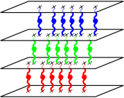
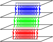
Figure 7: A string of stacks as $L$ approaches $\infty$. From left to right: $L$ small, $L$ large, thermodynamic limit.

The Bethe equations are obtained by the usual procedure, but applied to the stacks, rather than to individual roots: when a stack makes a tour around the chain its scattering phase after interaction with all other stacks is $2\pi\mathbb{Z}$, due to the periodicity:

$$-\sum_{k^{\prime}=1}^{7}\sum_{l^{\prime}=k^{\prime}+1}^{8}M_{kl,k^{\prime}l^{\prime}}\makebox[0.0pt][l]{\hskip 0.59998pt$/$}G_{k^{\prime}l^{\prime}}(u)-\frac{V_{kl}}{u}=2\pi n_{kl,a},\qquad\mbox{for }u\in\mathcal{C}_{kl,a}.$$ (4.16)

When we substitute (4.4,4.7) the above equation reads

$$-\eta_{k}\sum_{j=1}^{8}\makebox[0.0pt][l]{\hskip 0.59998pt$/$}G_{kj}(u)+\eta_{l}\sum_{j=1}^{8}\makebox[0.0pt][l]{\hskip 0.59998pt$/$}G_{lj}(u)-\frac{\varepsilon_{k}-\varepsilon_{l}}{2u}=2\pi n_{kl,a},\qquad\mbox{for }u\in\mathcal{C}_{kl,a}.$$ (4.17)

For convenience, we have defined all resolvents as antisymmetric in the stack indices $(k,l)$: $G_{lk}(u)=-G_{kl}(u)$. Here $\mathcal{C}_{kl,a}$ is a connected component of $\mathcal{C}_{kl}$ and $n_{kl,a}$ is the corresponding mode number. Note that we have used a slash to indicate a principal value prescription on all resolvents. In a given equation, it will however only be relevant for the resolvent $G_{kj}$ with the cut $\mathcal{C}_{kl,a}$. The remaining slashed resolvents coincide with their unslashed value.

Introduce the quasi-momenta

$$p_{k}(u)=\frac{\varepsilon_{k}}{2u}+\eta_{k}\sum_{l=1}^{8}G_{kl}(u)\,,\qquad k=1,\ldots,8.$$ (4.18)

These functions determine the eigenvalues of the transfer matrices, see App. A.4 and (A.16). They let us write the Bethe equations as

$$\makebox[0.0pt][l]{\hskip 0.59998pt$/$}p_{l}(u)-\makebox[0.0pt][l]{\hskip 0.59998pt$/$}p_{k}(u)=2\pi n_{kl,a},\qquad\mbox{for }u\in\mathcal{C}_{kl,a}.$$ (4.19)

4.5 Local and Global Charges

In the thermodynamic limit we can express the trace cyclicity (2.8), the one-loop anomalous dimension (2.9) and the higher integrable charges (2.10) in terms of the resolvents (4.14)

$$G_{\mathrm{mom}}(0)=2\pi m,\qquad\delta E=\frac{\lambda}{8\pi^{2}L}\,G_{\mathrm{mom}}^{\prime}(0).\qquad G_{\mathrm{mom}}(u)=\sum_{r=1}^{\infty}(Lu)^{r-1}Q_{r}.$$ (4.20)

Here, the combined resolvent $G_{\mathrm{mom}}(u)$ for momentum-carrying excitations reads

$$G_{\mathrm{mom}}(u)=\sum_{k=1}^{4}\sum_{l=5}^{8}G_{kl}(u).$$ (4.21)

Note that we can alternatively write the momentum-carrying resolvent using the quasi-momenta as

$$G_{\mathrm{mom}}(u)=\sum_{k=1}^{8}{\textstyle\frac{1}{2}}\eta_{k}\varepsilon_{k}p_{k}(u)=\sum_{k,l=1}^{8}{\textstyle\frac{1}{2}}\varepsilon_{k}G_{kl}(u).$$ (4.22)

As usual, the global charges are found in the asymptotics of the quasi-momenta $\tilde{p}_{k}(x)$ at $x=\infty$. The global charges associated to $S^{5}$ at $x=\infty$ are [63]

$$\tilde{p}_{1}(u)\mathrel{} = \mathrel{}\frac{1}{Lu}\left(+{\textstyle\frac{3}{4}}\tilde{r}_{1}+{\textstyle\frac{1}{2}}\tilde{r}_{2}+{\textstyle\frac{1}{4}}\tilde{r}_{3}+{\textstyle\frac{1}{4}}r^{\ast}\right)+\cdots\,,$$

$$\tilde{p}_{2}(u)\mathrel{} = \mathrel{}\frac{1}{Lu}\left(-{\textstyle\frac{1}{4}}\tilde{r}_{1}+{\textstyle\frac{1}{2}}\tilde{r}_{2}+{\textstyle\frac{1}{4}}\tilde{r}_{3}+{\textstyle\frac{1}{4}}r^{\ast}\right)+\cdots\,,$$

$$\tilde{p}_{3}(u)\mathrel{} = \mathrel{}\frac{1}{Lu}\left(-{\textstyle\frac{1}{4}}\tilde{r}_{1}-{\textstyle\frac{1}{2}}\tilde{r}_{2}+{\textstyle\frac{1}{4}}\tilde{r}_{3}+{\textstyle\frac{1}{4}}r^{\ast}\right)+\cdots\,,$$

$$\tilde{p}_{4}(u)\mathrel{} = \mathrel{}\frac{1}{Lu}\left(-{\textstyle\frac{1}{4}}\tilde{r}_{1}-{\textstyle\frac{1}{2}}\tilde{r}_{2}-{\textstyle\frac{3}{4}}\tilde{r}_{3}+{\textstyle\frac{1}{4}}r^{\ast}\right)+\cdots\,.$$ (4.23)

Here, $[\tilde{r}_{1},\tilde{r}_{2},\tilde{r}_{3}]$ are the the Dynkin labels of $\mathfrak{su}(4)$ related to orthogonal spins $J_{1,2,3}$ of $\mathfrak{so}(6)$ by $\tilde{r}_{1}=J_{2}-J_{3}$, $\tilde{r}_{2}=J_{1}-J_{2}$, $\tilde{r}_{3}=J_{2}+J_{3}$. Similarly, in the $\mathfrak{su}(2,2)$ sector [66]

$$\hat{p}_{1}(u)\mathrel{} = \mathrel{}-\frac{1}{Lu}\left(+{\textstyle\frac{3}{4}}\hat{r}_{1}+{\textstyle\frac{1}{2}}\hat{r}_{2}+{\textstyle\frac{1}{4}}\hat{r}_{3}-{\textstyle\frac{1}{4}}r^{\ast}\right)+\cdots\,,$$

$$\hat{p}_{2}(u)\mathrel{} = \mathrel{}-\frac{1}{Lu}\left(-{\textstyle\frac{1}{4}}\hat{r}_{1}+{\textstyle\frac{1}{2}}\hat{r}_{2}+{\textstyle\frac{1}{4}}\hat{r}_{3}-{\textstyle\frac{1}{4}}r^{\ast}\right)+\cdots\,,$$

$$\hat{p}_{3}(u)\mathrel{} = \mathrel{}-\frac{1}{Lu}\left(-{\textstyle\frac{1}{4}}\hat{r}_{1}-{\textstyle\frac{1}{2}}\hat{r}_{2}+{\textstyle\frac{1}{4}}\hat{r}_{3}-{\textstyle\frac{1}{4}}r^{\ast}\right)+\cdots\,,$$

$$\hat{p}_{4}(u)\mathrel{} = \mathrel{}-\frac{1}{Lu}\left(-{\textstyle\frac{1}{4}}\hat{r}_{1}-{\textstyle\frac{1}{2}}\hat{r}_{2}-{\textstyle\frac{3}{4}}\hat{r}_{3}-{\textstyle\frac{1}{4}}r^{\ast}\right)+\cdots\,.$$ (4.24)

The Dynkin labels $[\hat{r}_{1},\hat{r}_{2},\hat{r}_{3}]$ of $\mathfrak{su}(2,2)$ are related to orthogonal spins $(S_{1,2},E)$ of $\mathfrak{so}(2,4)$ by $\hat{r}_{1}=S_{1}-S_{2}$, $\hat{r}_{2}=-E-S_{1}$, $\hat{r}_{3}=S_{1}+S_{2}$. The relation to the fillings reads for $\mathfrak{su}(4)$

$$\begin{array}[]{rclcrcl}\tilde{r}_{1}\mathrel{}&=&\mathrel{}\tilde{K}_{2}-2\tilde{K}_{1},&&\tilde{K}_{1}\mathrel{}&=&\mathrel{}{\textstyle\frac{1}{2}}L-{\textstyle\frac{3}{4}}\tilde{r}_{1}-{\textstyle\frac{1}{2}}\tilde{r}_{2}-{\textstyle\frac{1}{4}}\tilde{r}_{3},\\[3.01385pt] \tilde{r}_{2}\mathrel{}&=&\mathrel{}L-2\tilde{K}_{2}+\tilde{K}_{1}+\tilde{K}_{3},&&\tilde{K}_{2}\mathrel{}&=&\mathrel{}\phantom{{\textstyle\frac{1}{2}}}L-{\textstyle\frac{1}{2}}\tilde{r}_{1}-\phantom{{\textstyle\frac{1}{2}}}\tilde{r}_{2}-{\textstyle\frac{1}{2}}\tilde{r}_{3},\\[3.01385pt] \tilde{r}_{3}\mathrel{}&=&\mathrel{}\tilde{K}_{2}-2\tilde{K}_{3},&&\tilde{K}_{3}\mathrel{}&=&\mathrel{}{\textstyle\frac{1}{2}}L-{\textstyle\frac{1}{4}}\tilde{r}_{1}-{\textstyle\frac{1}{2}}\tilde{r}_{2}-{\textstyle\frac{3}{4}}\tilde{r}_{3}.\end{array}$$ (4.25)

and for $\mathfrak{su}(2,2)$ correspondingly

$$\begin{array}[]{rclcrcl}\hat{r}_{1}\mathrel{}&=&\mathrel{}\hat{K}_{2}-2\hat{K}_{1},&&\hat{K}_{1}\mathrel{}&=&\mathrel{}-{\textstyle\frac{1}{2}}L-{\textstyle\frac{1}{2}}\delta E-{\textstyle\frac{3}{4}}\hat{r}_{1}-{\textstyle\frac{1}{2}}\hat{r}_{2}-{\textstyle\frac{1}{4}}\hat{r}_{3},\\[3.01385pt] \hat{r}_{2}\mathrel{}&=&\mathrel{}-L-\delta E-2\hat{K}_{2}+\hat{K}_{1}+\hat{K}_{3},&&\hat{K}_{2}\mathrel{}&=&\mathrel{}-\phantom{{\textstyle\frac{1}{2}}}L-\phantom{{\textstyle\frac{1}{2}}}\delta E-{\textstyle\frac{1}{2}}\hat{r}_{1}-\phantom{{\textstyle\frac{1}{2}}}\hat{r}_{2}-{\textstyle\frac{1}{2}}\hat{r}_{3},\\[3.01385pt] \hat{r}_{3}\mathrel{}&=&\mathrel{}\hat{K}_{2}-2\hat{K}_{3},&&\hat{K}_{3}\mathrel{}&=&\mathrel{}-{\textstyle\frac{1}{2}}L-{\textstyle\frac{1}{2}}\delta E-{\textstyle\frac{1}{4}}\hat{r}_{1}-{\textstyle\frac{1}{2}}\hat{r}_{2}-{\textstyle\frac{3}{4}}\hat{r}_{3}.\end{array}$$ (4.26)

Note that the Dynkin labels can be obtained as

$$\tilde{r}_{j}\mathrel{} = \mathrel{}\frac{L}{2\pi i}\oint_{\infty}du\,\bigl{(}\tilde{p}_{j}(u)-\tilde{p}_{j+1}(u)\bigr{)}.$$

$$\hat{r}_{j}\mathrel{} = \mathrel{}\frac{L}{2\pi i}\oint_{\infty}du\,\bigl{(}\hat{p}_{j+1}(u)-\hat{p}_{j}(u)\bigr{)}.$$ (4.27)

4.6 Separation into $\mathfrak{su}(4)$ and $\mathfrak{su}(2,2)$

As emphasized above, fermionic stacks are solitary and therefore irrelevant in the leading approximation of thermodynamic limit. Let us now write the Bethe equations in a form where the distinction between fermions and bosons becomes more apparent. We shall distinguish the quasi-momenta by their grading in the two sets $\tilde{p}=\{p_{3},p_{4},p_{5},p_{6}\}$ corresponding to $\mathfrak{su}(4)$ and $\hat{p}=\{p_{1},p_{2},p_{7},p_{8}\}$ corresponding to $\mathfrak{su}(2,2)$. In what follows we will denote them as

$$\begin{array}[b]{rclcrclcrclcrcl}p_{3}\mathrel{}&\equiv&\mathrel{}\tilde{p}_{1},&p_{4}\mathrel{}&\equiv&\mathrel{}\tilde{p}_{2},&p_{5}\mathrel{}&\equiv&\mathrel{}\tilde{p}_{3},&p_{6}\mathrel{}&\equiv&\mathrel{}\tilde{p}_{4},\\[4.0pt] p_{1}\mathrel{}&\equiv&\mathrel{}\hat{p}_{1},&p_{2}\mathrel{}&\equiv&\mathrel{}\hat{p}_{2},&p_{7}\mathrel{}&\equiv&\mathrel{}\hat{p}_{3},&p_{8}\mathrel{}&\equiv&\mathrel{}\hat{p}_{4}.\end{array}$$ (4.28)

In the same way we introduce three types of resolvents $\tilde{G}_{kl}(u)$ corresponding to bosons of $\mathfrak{su}(4)$, $\hat{G}_{kl}(u)$ corresponding to bosons of $\mathfrak{su}(2,2)$ and $G^{\ast}_{kl}(u)$ corresponding to fermions:

$$G_{kl}\mathrel{} \equiv \mathrel{}\tilde{G}_{k^{\prime}l^{\prime}},\quad\mbox{for }k,l=3,4,5,6,$$

$$G_{kl}\mathrel{} \equiv \mathrel{}\hat{G}_{k^{\prime}l^{\prime}},\quad\mbox{for }k,l=1,2,7,8,$$

$$G_{kl}\mathrel{} \equiv \mathrel{}G^{\ast}_{k^{\prime}l^{\prime}},\quad\mbox{for }k=3,4,5,6\mbox{ and }l=1,2,7,8,$$ (4.29)

where the primed indices are related to the unprimed ones corresponding to (4.28). In the leading approximation of the thermodynamic limit, the fermionic resolvents are irrelevant, $G^{\ast}_{kl}=\mathcal{O}(1/L)$, and we could set them to zero. Let us nevertheless carry them along to preserve the full supersymmetric structure.

These resolvents obey three sets of independent equations:

• The Bethe equations for $\mathfrak{su}(4)$ flavor excitations read

  $$\makebox[0.0pt][l]{\hskip 0.59998pt$/$}\tilde{p}_{l}(u)-\makebox[0.0pt][l]{\hskip 0.59998pt$/$}\tilde{p}_{k}(u)=2\pi\tilde{n}_{kl,a}\qquad\mbox{for }u\in\tilde{\mathcal{C}}_{kl,a},\qquad 1\leq k<l\leq 4$$ (4.30)

  where

  $$\tilde{p}_{k}(u)=\sum_{l=1}^{4}\tilde{G}_{kl}(u)+\sum_{l=1}^{4}G^{\ast}_{kl}(u)+\frac{\varepsilon_{k}}{2u}\,,\qquad k=1,\ldots,4.$$ (4.31)

  Here we have defined the reduced form of $\varepsilon_{k}$ as $\varepsilon_{k}=(+1,+1,-1,-1)$. Written in terms of resolvents, the Bethe equations read

  $$\sum_{j=1}^{4}\bigl{(}-\makebox[0.0pt][l]{\hskip 0.59998pt$/$}\tilde{G}_{kj}(u)+\makebox[0.0pt][l]{\hskip 0.59998pt$/$}\tilde{G}_{lj}(u)-G^{\ast}_{kj}(u)+G^{\ast}_{lj}(u)\bigr{)}-\frac{\varepsilon_{k}-\varepsilon_{l}}{2u}=2\pi\tilde{n}_{kl,a}\quad\mbox{for }u\in\tilde{\mathcal{C}}_{kl,a}.$$ (4.32)

• The Bethe equations for $\mathfrak{su}(2,2)$ derivative excitations read

  $$\makebox[0.0pt][l]{\hskip 0.59998pt$/$}\hat{p}_{l}(u)-\makebox[0.0pt][l]{\hskip 0.59998pt$/$}\hat{p}_{k}(u)=2\pi\hat{n}_{kl,a}\qquad\mbox{for }u\in\hat{\mathcal{C}}_{kl,a},\qquad 1\leq k<l\leq 4,$$ (4.33)

  where

  $$\hat{p}_{k}(u)=\sum_{l=1}^{4}\hat{G}_{lk}(u)+\sum_{l=1}^{4}G^{\ast}_{lk}(u)+\frac{\varepsilon_{k}}{2u}\,.$$ (4.34)

  Using resolvents, the Bethe equations become

  $$\sum_{j=1}^{4}\bigl{(}-\makebox[0.0pt][l]{\hskip 0.59998pt$/$}\hat{G}_{jk}(u)+\makebox[0.0pt][l]{\hskip 0.59998pt$/$}\hat{G}_{jl}(u)-G^{\ast}_{jk}(u)+G^{\ast}_{jl}(u)\bigr{)}-\frac{\varepsilon_{k}-\varepsilon_{l}}{2u}=2\pi\hat{n}_{kl,a}\quad\mbox{for }u\in\hat{\mathcal{C}}_{kl,a}.$$ (4.35)

• The Bethe equations for fermionic excitations read

  $$\makebox[0.0pt][l]{\hskip 0.59998pt$/$}\hat{p}_{l}(u)-\makebox[0.0pt][l]{\hskip 0.59998pt$/$}\tilde{p}_{k}(u)=2\pi n^{\ast}_{kl,a}\qquad\mbox{for }u=u^{\ast}_{kl,a},\qquad 1\leq k,l\leq 4.$$ (4.36)

The momentum-carrying resolvent determines the momentum, energy and local charges of a solution, c.f. (4.20), becomes

$$G_{\mathrm{mom}}=\sum_{k,l=1}^{4}{\textstyle\frac{1}{2}}\varepsilon_{k}\bigl{(}\tilde{G}_{kl}-\hat{G}_{lk}+G^{\ast}_{kl}-G^{\ast}_{lk}\bigr{)}.$$ (4.37)

Now let us switch off the fermions by setting $G^{\ast}_{kl}=0$. Then we see that the Bethe equations for the flavor and derivative sectors (4.32,4.35) become fully independent. Moreover these equations are very similar, they merely differ by the order of indices of resolvents $\tilde{G}_{kl}$ and $\hat{G}_{lk}$. When we order them in the same way, we see that effectively the potential term $(\varepsilon_{k}-\varepsilon_{l})/u$ changes sign. Nevertheless, the two sectors are not completely independent but they are related through the momentum constraint $G_{\mathrm{mom}}(0)=2\pi m$ with $G_{\mathrm{mom}}(u)$ defined in (4.37). Furthermore, the energy and local charges are the sums of energy and local charges in both sectors.

In Sec. 4.8 we present an even more particular case of Bethe equations only for $1+1|4$ modes in the $\mathfrak{su}(1,1|2)$ sector.

4.7 Fermions and Solitary Bosons

Let us now discuss the role of fermions in the thermodynamic limit. As mentioned above, fermionic stacks cannot form strings. The reason is the exclusion principle for Bethe roots in combination with the absence of repulsion for fermionic stacks. The absence of repulsion is the trivial consequence of the absence of self-scattering terms among fermionic stacks. In such a fermionic would-be string all the stacks would fall onto the minimum of the effective potential created by the bare potential $\pm 1/u+2\pi n$ and the Coulomb interaction with a given bosonic background. It follows from these arguments that one can have only solitary fermionic stacks at a given position in the $u$-plane. Such fermionic excitations have no influence on the bosonic background in the leading order for $L\to\infty$. The corresponding resolvents, consisting from a few poles at the positions of the fermionic stacks, can be dropped from Bethe equations since the residues at the poles are $\mathcal{O}(1/L)$. However, in the main order a meaningful problem is to find the positions of these fermionic poles. In particular, this is useful for the derivation of the spectrum of excitations of the bosonic background which is $\mathcal{O}(1/L)$.

The simplest example of such solitary fermionic roots is given by the purely fermionic $\mathfrak{u}(1|1)$ sector of the $\mathcal{N}=4$ SYM theory: The positions $u_{n}$ of roots are given by the equation [80]

$$\left(\frac{u+\frac{i}{2}}{u-\frac{i}{2}}\right)^{L}=1,$$ (4.38)

or in the thermodynamic limit

$$L/u_{n}=2\pi n,\qquad n\in\mathbb{Z}.$$ (4.39)

Here the effective potential coincides with the bare one and the fermions sit at its minima, no more than one in each.

Let us note that we can also consider solitary bosonic stacks, or very short strings consisting of them. This case does not differ significantly from the fermionic one: such short cuts do not contribute in the main order of the thermodynamic limit and the corresponding resolvents (consisting of a few pole terms) should be dropped from the Bethe equations.

We can find the positions of such fermionic or solitary bosonic $(k,l)$-stacks for a bosonic background given by a solution of (4.32,4.35,4.36). They are the solutions $u$ of the equation

$$p_{l}(u)-p_{k}(u)=2\pi n,$$ (4.40)

with $p_{k}(u)$ defined in (4.28,4.31,4.34). Here there is no principal value prescription since the solitary stack is not considered part of the quasi-momentum.

For an honest $\mathcal{O}(1/L)$ computation of the energy shift induced by adding a solitary stack, one must also take into account the deformation of the bosonic background. Luckily, the deformation does not influence the leading order position $u$ of the solitary excitation, but it has an effect on the energy and needs to be investigated. This is however beyond the scope of the current work.

4.8 The $\mathfrak{su}(1,1|2)$ Sector

Let us review the above arguments to derive the thermodynamic limit for the somewhat simpler $\mathfrak{su}(1,1|2)$ Bethe equations (3.4). Of course, all the derived equation equally follow by restriction of the results in the previous subsections. Consider first $K_{v}=K_{w}=K_{u}-1$, which corresponds to the $\mathfrak{sl}(2)$ sector after dualization. The middle equation then has a unique solution which allows one to express $v_{p}=w_{p}$’s in terms of $u_{q}$’s and reduce the Bethe equations to the $\mathfrak{sl}(2)$ form. How does this solution look like in the thermodynamic limit? We have to assume that $v_{p}\sim\mathcal{O}(L)$, otherwise the energy will be too high. However, a short inspection of the first equation shows that there is only finite number of solutions with $v_{p}\sim\mathcal{O}(L)$ and $v_{p}-u_{q}=\mathcal{O}(L)$. We have to relax the latter condition in order to allow for a macroscopically large number of $v$-roots. Therefore, the $v$-roots settle close to the $u$-roots and form stacks in the thermodynamic limit.

Figure 8: All six types of stacks for the $\mathfrak{su}(1,1|2)$ sector. The outer four stacks are momentum-carrying, the inner two are auxiliary. For each type of stack, we have indicated the corresponding resolvent.

In the pure $\mathfrak{sl}(2)$ case all roots (except one) will be combined into stacks of three: triples $(v_{p},u_{p},w_{p})$, $p=1,\ldots,K_{v}=K_{w}$. Conversely, in the $\mathfrak{su}(2)$ case there is only one flavor of roots. In a more general situation we have $\hat{K}$ stacks of all flavors and $\tilde{K}$ single roots of flavor $2$, c.f. Fig. 8. These two types of stacks are bosonic, are allowed to form strings and we introduce the corresponding integral resolvents

$$\hat{G}(u)=\int_{\tilde{\mathcal{C}}}\frac{dv\,\tilde{\rho}(v)}{v-u}\,,\qquad\tilde{G}(u)=\int_{\hat{\mathcal{C}}}\frac{dv\,\hat{\rho}(v)}{v-u}\,.$$ (4.41)

In addition, there can be finitely many fermionic stacks characterized by the discrete resolvents with $k,l=1,2$

$$G^{\ast}_{kl}(u)=\sum_{p=1}^{K^{\ast}_{kl}}\frac{1/L}{u^{\ast}_{kl,p}-u}\,.\qquad$$ (4.42)

We begin with the Bethe equation for roots of flavor $2$. This is given by the middle equation in (3.4) and the limit is

$$2\pi\tilde{n}_{p}+\frac{L}{u_{p}}=\sum_{q=1}^{K_{v}}\frac{1}{v_{q}-u_{p}}-\sum_{\textstyle\genfrac{}{}{0.0pt}{}{q=1}{q\neq p}}^{K_{u}}\frac{2}{u_{q}-u_{p}}+\sum_{q=1}^{K_{w}}\frac{1}{w_{q}-u_{p}}.$$ (4.43)

To turn the sums into the resolvents, we have to replace a sum over $v_{p}$ by $-G^{\ast}_{21}(u)-G^{\ast}_{11}(u)+\hat{G}(u)$, a sum over $u_{p}$ becomes $\tilde{G}(u)-G^{\ast}_{21}(u)+G^{\ast}_{12}(u)+\hat{G}(u)$ and finally the $w_{p}$-sums yield $G^{\ast}_{22}(u)-G^{\ast}_{21}(u)+\hat{G}(u)$, see Fig. 8. The resulting Bethe equation reads

$$2\pi\tilde{n}_{a}+\frac{1}{u}=-2\makebox[0.0pt][l]{\hskip 0.59998pt$/$}\tilde{G}(u)-G^{\ast}_{11}(u)-G^{\ast}_{12}(u)+G^{\ast}_{21}(u)+G^{\ast}_{22}(u)\quad\mbox{for }u\in\tilde{\mathcal{C}}_{a}.$$ (4.44)

Note that there is no anomaly for a single flavor of roots as explained in App. C. Also note that the term $\hat{G}(u)$ has dropped out from the equations since it has no common label with $\tilde{G}(u)$. To obtain the Bethe equation for stacks of three we first multiply all three Bethe equations and then take the limit (assuming that a stack is labelled by a common index $p$ for $u_{p}\approx v_{p}\approx w_{p}$)

$$2\pi\hat{n}_{p}+\frac{L}{u_{p}}=+\sum_{q=1}^{K_{u}}\frac{1}{u_{q}-v_{p}}+\sum_{q=1}^{K_{v}}\frac{1}{v_{q}-u_{p}}-\sum_{\textstyle\genfrac{}{}{0.0pt}{}{q=1}{q\neq p}}^{K_{u}}\frac{2}{u_{q}-u_{p}}+\sum_{q=1}^{K_{w}}\frac{1}{w_{q}-u_{p}}+\sum_{q=1}^{K_{u}}\frac{1}{u_{q}-w_{p}}.$$ (4.45)

In terms of resolvents we obtain

$$2\pi\hat{n}_{a}+\frac{1}{u}=+2\makebox[0.0pt][l]{\hskip 0.59998pt$/$}\hat{G}(u)-G^{\ast}_{11}(u)-G^{\ast}_{21}(u)+G^{\ast}_{12}(u)+G^{\ast}_{22}(u)\quad\mbox{for }u\in\hat{\mathcal{C}}_{a}.$$ (4.46)

Although the individual Bethe equations are anomalous, their product is anomaly-free, c.f. App. C. The equations which determine the position of the fermionic stacks are determined in a similar fashion:

$$2\pi n^{\ast}_{11,a}\mathrel{} = \mathrel{}+\tilde{G}(u)+\hat{G}(u)-G^{\ast}_{21}(u)+G^{\ast}_{12}(u)\quad\mbox{for }u=u^{\ast}_{11,a},$$

$$2\pi n^{\ast}_{21,a}+\frac{1}{u}\mathrel{} = \mathrel{}-\tilde{G}(u)+\hat{G}(u)-G^{\ast}_{11}(u)+G^{\ast}_{22}(u)\quad\mbox{for }u=u^{\ast}_{21,a},$$

$$2\pi n^{\ast}_{12,a}+\frac{1}{u}\mathrel{} = \mathrel{}-\tilde{G}(u)+\hat{G}(u)-G^{\ast}_{11}(u)+G^{\ast}_{22}(u)\quad\mbox{for }u=u^{\ast}_{12,a},$$

$$2\pi n^{\ast}_{22,a}\mathrel{} = \mathrel{}+\tilde{G}(u)+\hat{G}(u)-G^{\ast}_{21}(u)+G^{\ast}_{12}(u)\quad\mbox{for }u=u^{\ast}_{22,a},$$ (4.47)

In the leading order, we can drop the contribution from the finitely many fermions. The equations for the remaining bosonic modes can be written as

$$-2\pi\tilde{n}_{a}-\frac{1}{u}\mathrel{} = \mathrel{}2\makebox[0.0pt][l]{\hskip 0.59998pt$/$}\tilde{G}(u)\quad\mbox{for }u\in\tilde{\mathcal{C}}_{a},$$

$$2\pi\hat{n}_{a}+\frac{1}{u}\mathrel{} = \mathrel{}2\makebox[0.0pt][l]{\hskip 0.59998pt$/$}\hat{G}(u)\quad\mbox{for }u\in\hat{\mathcal{C}}_{a}.$$ (4.48)

These are two independent equations for $\mathfrak{sl}(2)$ and $\mathfrak{su}(2)$ densities, which are only coupled through the common momentum constraint and through the common expression for the energy

$$\tilde{G}(0)+\hat{G}(0)=2\pi m,\qquad\delta D=\frac{\lambda}{8\pi^{2}L}\,\bigl{(}\tilde{G}^{\prime}(0)+\hat{G}^{\prime}(0)\bigr{)}.$$ (4.49)

5 Algebraic Curve

Figure 9: Some configuration of cuts and poles for the sigma model. Cuts $\tilde{\mathcal{C}}_{a}$ between the sheets $\tilde{p}_{k}$ correspond to $S^{5}$ excitations and likewise cuts $\hat{\mathcal{C}}_{a}$ between the sheets $\hat{p}_{k}$ correspond to $AdS^{5}$ excitations. Poles $x^{\ast}_{a}$ on sheets $\tilde{p}_{k}$ and $\hat{p}_{l}$ correspond to fermionic excitations. The dashed line in the middle is related to physical excitations, cuts and poles which cross it contribute to the total momentum, energy shift and local charges.

We are now in position to construct the complete algebraic curve of the one-loop $\mathcal{N}=4$ SYM theory in the thermodynamic limit, in analogy with the full $AdS_{5}\times S^{5}$ curve of the string theory built in [64]. Note that if we drop the fermions, the problem is not principally new: the bosonic $\mathfrak{su}(4)$ and $\mathfrak{su}(2,2)$ sectors are almost completely factorized and each one is described by a separate curve of degree four.

As shown in [63], the $\mathfrak{su}(4)$ spectral curve has the form

$$\tilde{F}(\tilde{y},u)=\tilde{F}_{4}(u)\,\tilde{y}^{4}+\tilde{F}_{2}(u)\,\tilde{y}^{2}+\tilde{F}_{1}(u)\,\tilde{y}+\tilde{F}_{0}(u)=0$$ (5.1)

where

$$\tilde{y}(u)=u^{2}\,\tilde{p}^{\prime}(u).$$ (5.2)

For a curve with $\tilde{A}$ branch cuts, the leading coefficient $\tilde{F}_{4}(u)=\prod_{a=1}^{\tilde{A}}(u-\tilde{u}^{+}_{a})(u-\tilde{u}^{-}_{a})$ encodes the full information about all $2\tilde{A}$ branch points $\tilde{u}^{\pm}_{a}$ of the curve. Furthermore, the coefficient of $y^{3}$, $\tilde{F}_{3}(u)=0$ due to unimodularity $\tilde{p}_{1}(u)+\tilde{p}_{2}(u)+\tilde{p}_{3}(u)+\tilde{p}_{4}(u)=0$ of the monodromy matrix in this sector. In a $\mathfrak{su}(2,2)$ sector the situation is similar. The algebraic curve is given by [66]

$$\hat{F}(\hat{y},u)=\hat{F}_{4}(u)\,\hat{y}^{4}+\hat{F}_{2}(u)\,\hat{y}^{2}+\hat{F}_{1}(u)\,\hat{y}+\hat{F}_{0}(u)=0,$$ (5.3)

where again $\hat{F}_{4}(u)=\prod_{a=1}^{\hat{A}}(u-\hat{u}_{a}^{+})(u-\hat{u}_{a}^{-})$ encodes the full information about the $2\hat{A}$ branch points $\hat{u}^{\pm}_{a}$ of the curve. Note that $\hat{F}_{3}(u)=0$ since $\hat{p}_{1}(u)+\hat{p}_{2}(u)+\hat{p}_{3}(u)+\hat{p}_{4}(u)=0$.

The supersymmetric curve can be represented, in analogy with the string algebraic curve [64], in a rational form reflecting the characteristic rational function of a supermatrix (as opposed to a characteristic polynomial of a regular matrix)

$$F(y,u)=\frac{\tilde{F}_{4}(u)\,y^{4}+\tilde{F}_{3}(u)\,y^{3}+\tilde{F}_{2}(u)\,y^{2}+\tilde{F}_{1}(u)\,y+\tilde{F}_{0}(u)}{\hat{F}_{4}(u)\,y^{4}+\hat{F}_{3}(u)\,y^{3}+\hat{F}_{2}(u)\,y^{2}+\hat{F}_{1}(u)\,y+\hat{F}_{0}(u)}\,,$$ (5.4)

with $\tilde{F}_{k}(u),\hat{F}_{k}(u)$ polynomials in $u$. The curve $y(u)=\{\tilde{y}(u)||\hat{y}(u)\}$ obeys the algebraic equations

$$\tilde{F}(\tilde{y}(u),u)=0,\qquad\hat{F}(\hat{y}(u),u)=0.$$ (5.5)

Note that now we have

$$\frac{\tilde{F}_{3}(u)}{\tilde{F}_{4}(u)}=\frac{\hat{F}_{3}(u)}{\hat{F}_{4}(u)}$$ (5.6)

since instead of the two unimodularity conditions we have only one superunimodularity condition

$$\tilde{p}_{1}(u)+\tilde{p}_{2}(u)+\tilde{p}_{3}(u)+\tilde{p}_{4}(u)-\hat{p}_{1}(u)-\hat{p}_{2}(u)-\hat{p}_{3}(u)-\hat{p}_{4}(u)=0.$$ (5.7)

The dynamical singularities are encoded in $F_{4}(u)$ as

$$\tilde{F}_{4}(u)\mathrel{} = \mathrel{}\prod_{a=1}^{\tilde{A}}(u-\tilde{u}^{+}_{a})\prod_{a=1}^{\tilde{A}}(u-\tilde{u}^{-}_{a})\prod_{a=1}^{A^{\ast}}(u-u^{\ast}_{a})^{2},$$

$$\hat{F}_{4}(u)\mathrel{} = \mathrel{}\prod_{a=1}^{\hat{A}}(u-\hat{u}^{+}_{a})\prod_{a=1}^{\hat{A}}(u-\hat{u}^{-}_{a})\prod_{a=1}^{A^{\ast}}(u-u^{\ast}_{a})^{2}.$$ (5.8)

For $\tilde{F}_{4}(u),\hat{F}_{4}(u)$ there are in total $2\tilde{A}+2\hat{A}+A^{\ast}$ degrees of freedom.

At $u=\infty$ and $u=0$ the curve $y(u)$ approaches finite limiting values. This is achieved by letting all the polynomials $\tilde{F}_{k}(u)$ have the same order $2\tilde{A}$ as well as all the $\hat{F}_{k}(u)$ have the order $2\hat{A}$. Note that the behavior of $\tilde{F}_{2,1,0},\hat{F}_{2,1,0}$ is generic at the zeroes of $\tilde{F}_{4},\hat{F}_{4}$. The number of free coefficients in all $\tilde{F}_{k}(u),\hat{F}_{k}(u)$, $k\leq 2$ is $6\tilde{A}+6\hat{A}+12A^{\ast}+6$. Adding the parameters of $\tilde{F}_{4}(u),\hat{F}_{4}(u)$ we get $8\tilde{A}+8\hat{A}+13A^{\ast}+6$ relevant coefficients.

The unimodularity condition (5.6) imposes

$$\tilde{F}_{3}(u)\mathrel{} = \mathrel{}F_{3}^{\ast}(u)\prod_{a=1}^{\tilde{A}}(u-\tilde{u}^{+}_{a})\prod_{a=1}^{\tilde{A}}(u-\tilde{u}^{-}_{a}),$$

$$\hat{F}_{3}(u)\mathrel{} = \mathrel{}F_{3}^{\ast}(u)\prod_{a=1}^{\hat{A}}(u-\hat{u}^{+}_{a})\prod_{a=1}^{\hat{A}}(u-\hat{u}^{-}_{a}),$$ (5.9)

with some polynomial $F_{3}^{\ast}(u)$ of order $2A^{\ast}$, which contributes $2A^{\ast}+1$ free coefficients. In total we now have $8\tilde{A}+8\hat{A}+15A^{\ast}+7$ free parameters. Let us see how they can be fixed.

Singularities.

The coefficient of the double pole in $\tilde{p}_{k}^{\prime},\hat{p}_{k}^{\prime}$ at $u=0$ is read from (4.31,4.34). In terms of $y(u)$ it appears as

$$\tilde{y}_{k}(u),\,\hat{y}_{k}(u)=-{\textstyle\frac{1}{2}}\varepsilon_{k}+\mathcal{O}(u).$$ (5.10)

These can be used to fix the relative ratios among the constant terms $\tilde{F}_{k}(0)$ as $\tilde{F}_{4}(0)=-2\tilde{F}_{2}(0)=16\tilde{F}_{0}(0),\$ $\tilde{F}_{3}(0)=\tilde{F}_{1}(0)=0$. The same constraints hold for $\hat{F}_{k}(0)$ except $\hat{F}_{3}(0)=0$, which is automatically satisfied since we have already imposed (5.6) in the ansatz (5). In total we have 7 constraints which reduce the total degrees of freedom to $8\tilde{A}+8\hat{A}+15A^{\ast}$.

Unphysical Branch Points.

In addition to the physical branch points at $\tilde{u}^{\pm}_{a},\hat{u}^{\pm}_{a}$ the algebraic curve might have further ones. Generically, these singularities are square roots in contrast to the physical ones which are inverse square roots. We can remove them using conditions on the discriminants

$$\tilde{R}\mathrel{} = \mathrel{}-4\tilde{F}_{1}^{2}\tilde{F}_{2}^{3}\tilde{F}_{4}+16\tilde{F}_{0}\tilde{F}_{2}^{4}\tilde{F}_{4}-27\tilde{F}_{1}^{4}\tilde{F}_{4}^{2}+144\tilde{F}_{0}\tilde{F}_{1}^{2}\tilde{F}_{2}\tilde{F}_{4}^{2}-128\tilde{F}_{0}^{2}\tilde{F}_{2}^{2}\tilde{F}_{4}^{2}+256\tilde{F}_{0}^{3}\tilde{F}_{4}^{3}$$ (5.11)

$$\mathord{}+18\tilde{F}_{1}^{3}\tilde{F}_{2}\tilde{F}_{3}\tilde{F}_{4}-80\tilde{F}_{0}\tilde{F}_{1}\tilde{F}_{2}^{2}\tilde{F}_{3}\tilde{F}_{4}-192\tilde{F}_{0}^{2}\tilde{F}_{1}\tilde{F}_{3}\tilde{F}_{4}^{2}-6\tilde{F}_{0}\tilde{F}_{1}^{2}\tilde{F}_{3}^{2}\tilde{F}_{4}+144\tilde{F}_{0}^{2}\tilde{F}_{2}\tilde{F}_{3}^{2}\tilde{F}_{4}$$

$$\mathord{}+\tilde{F}_{1}^{2}\tilde{F}_{2}^{2}\tilde{F}_{3}^{2}-4\tilde{F}_{0}\tilde{F}_{2}^{3}\tilde{F}_{3}^{2}-4\tilde{F}_{1}^{3}\tilde{F}_{3}^{3}+18\tilde{F}_{0}\tilde{F}_{1}\tilde{F}_{2}\tilde{F}_{3}^{3}-27\tilde{F}_{0}^{2}\tilde{F}_{3}^{4}$$

and similarly for $\hat{R}$. The discriminants must have the form

$$\tilde{R}(u)\mathrel{} = \mathrel{}\prod_{a=1}^{\tilde{A}}(u-\tilde{u}^{+}_{a})\prod_{a=1}^{\tilde{A}}(u-\tilde{u}^{-}_{a})\,\tilde{Q}(u)^{2},$$

$$\hat{R}(u)\mathrel{} = \mathrel{}\prod_{a=1}^{\hat{A}}(u-\hat{u}^{+}_{a})\prod_{a=1}^{\hat{A}}(u-\hat{u}^{-}_{a})\,\hat{Q}(u)^{2}.$$ (5.12)

It is clear that $\tilde{u}^{\pm}_{a}$ and $\hat{u}^{\pm}_{a}$ are roots, because all terms in (5.11) contain $\tilde{F}_{4}$ or $\tilde{F}_{3}$. The degree of the polynomials $\hat{Q},\tilde{Q}$ is $5\tilde{A}+6A^{\ast}$ and $5\hat{A}+6A^{\ast}$, respectively. This special form of discriminants removes $5\tilde{A}+5\hat{A}+12A^{\ast}$ parameters and the remaining number of degrees of freedom is $3\tilde{A}+3\hat{A}+3A^{\ast}$.

Single Poles and A-Cycles.

We need to remove all the single poles to avoid undesired logarithmic behavior in the quasi-momentum. We can put all the integrals of $dp(u)$ around A-cycles to be zero

$$\oint_{\mathcal{A}_{a}}d\tilde{p}=0,$$ (5.13)

as explained in [60]. There are $\tilde{A}+\hat{A}$ A-cycles around bosonic cuts. Fermionic singularities contribute $2A^{\ast}$ independent single poles: One for $\tilde{y}$ and one for $\hat{y}$ at each $u=u^{\ast}_{a}$. At $u=0$, the curve $y(u)$ has a double pole but no single pole. This amounts to further $7$ constraints. Among all these single poles and A-cycles, there are $7$ relations from the sum over all residues on all independent sheets. In total the single-valuedness of $p(u)$ yields $\tilde{A}+\hat{A}+2A^{\ast}$ constraints and leaves $2\tilde{A}+2\hat{A}+A^{\ast}$ coefficients.

B-Periods.

For each bosonic cut and for each fermionic singularity there is a B-period. Due to the Bethe equations (4.30,4.33,4.36) it must be an integral multiple of $2\pi$

$$\int_{\mathcal{B}_{a}}dp=2\pi n_{a}.$$ (5.14)

In total we obtain $\tilde{A}+\hat{A}+A^{\ast}$ constraints and are left with $\tilde{A}+\hat{A}$ degrees of freedom.

Cyclicity.

Finally we should not forget the momentum constraint in (4.20)

$$q(0)=2\pi m,\qquad q(u)=\sum_{k=1}^{4}\varepsilon_{k}\bigl{(}\tilde{p}_{k}(u)-\hat{p}_{k}(u)\bigr{)}=G_{\mathrm{mom}}(u)$$ (5.15)

selecting curves with an integer winding number $m$. In total the admissible algebraic curves for one-loop gauge theory have $\tilde{A}+\hat{A}-1$ continuous moduli.

Let us just repeat (4.20), which defines the energy shift $\delta E$ and local charges $Q_{r}$, in terms of the generating function $q(u)$

$$\delta E=\frac{\lambda}{8\pi^{2}L}\,q^{\prime}(0).\qquad q(u)=\sum_{r=1}^{\infty}(Lu)^{r-1}Q_{r}.$$ (5.16)

Fillings.

We can now associate a particular integral around a cut, the filling, to each of the moduli

$$\tilde{K}_{kl,a}\mathrel{} = \mathrel{}-\frac{L}{2\pi i}\oint_{\tilde{\mathcal{A}}_{kl,a}}\tilde{p}_{k}(u)\,du,$$

$$\hat{K}_{kl,a}\mathrel{} = \mathrel{}-\frac{L}{2\pi i}\oint_{\hat{\mathcal{A}}_{kl,a}}\hat{p}_{l}(u)\,du,$$

$$K^{\ast}_{kl,a}\mathrel{} = \mathrel{}-\frac{L}{2\pi i}\oint_{{\mathcal{A}}^{\ast}_{kl,a}}\tilde{p}_{k}(u)\,du.$$ (5.17)

For completeness, we have defined fillings for fermionic poles as well, they must equal $1$. The fillings obey the constraint

$$\sum_{a=1}^{A}n_{a}K_{a}=mL$$ (5.18)

which can be derived from the Bethe equations (4.17) by integrating/summing over all cuts/poles. This reduces the number of independent fillings by one, in compliance with the total number of independent moduli.

Supersymmetric Landau-Lifshitz Model.

We would like to note that the curve discussed in this section is most likely the spectral curve of the generalized Landau-Lifshitz model proposed in [49]. This model appears to arise as the coherent-state picture in the thermodynamic limit of one-loop gauge theory. It seems to be a rather straight-forward generalization of the $\mathrm{SU}(2)/\mathrm{U}(1)$ coherent-state model in [47] to the larger and supersymmetric coset $\mathrm{PSU}(2,2|4)/\mathrm{PSU}(2|2)^{2}\times\mathrm{U}(1)^{2}$. For the smaller model, the Heisenberg magnet, the finite-gap solution was constructed in [60]. Like the above curve, this one has only one singularity at $u=0$ and $\mathfrak{psu}(2,2|4)$ symmetry generators at $u=\infty$. Furthermore, the highest weight state $\mathcal{Z}$ is invariant under $\mathrm{PSU}(2|2)^{2}$ and thus the residues $\varepsilon_{k}/2$ at $u=0$ should match. It would be interesting to construct some local charges of the supersymmetric Landau-Lifshitz model which arise in the expansion around $u=0$.

6 Comparison to String Theory

6.1 Spectral Curves

Now we will show that the most general algebraic curve of the SYM theory at one loop, constructed in the last section, coincides with that of the string sigma model [64] in the Frolov–Tseytlin limit $\lambda/L^{2}\to 0$ (see Sec. 3.7 of [64]). This coincidence was already observed for particular sectors in [60, 61, 63].

As in [63] we compare the analytical data defining the structure and the moduli of both curves in terms of a rescaled variable $u$ which is defined as $u=(\sqrt{\lambda}/4\pi L)\,x$ for the strings and is similar to the spectral parameter $u$ used through this paper. The parameter of “length” $L$ for strings was introduced in Sec. 3.3 of [64] as a modulus satisfying the equivalent of the constraint (5.18).

The algebraic curve for the string sigma model exhibits an inversion symmetry $x\mapsto 1/x$ with respect to the coordinate $x$ and all the branch points and fermionic poles form mutually symmetric pairs. In terms of the coordinate $u$ they can be expressed as

$$(u_{a},u_{A+a})=\left(u_{a},\frac{\lambda}{16\pi^{2}L^{2}}\,\frac{1}{u_{a}}\right),\quad a=1,\ldots,A$$ (6.1)

where we abbreviate $\tilde{u}_{a}^{\pm},\tilde{A}$, $\hat{u}_{a}^{\pm},\hat{A}$ or $u_{a}^{*},A^{*}$ by $u_{a},A$. In the Frolov–Tseytlin limit, the $u_{a}$’s remain finite while the $u_{A+a}$’s go to zero. This means that in the $x$-plane half of the cuts/poles approach $x=\infty$ and half of them approach $x=0$. We will concentrate our attention on that half of the cuts/poles which remain finite in the $u$-plane: $\tilde{\mathcal{C}}_{a},\ a=1,\ldots,\tilde{A}$, $\hat{\mathcal{C}}_{a},\ a=1,\ldots,\hat{A}$ and $u_{a}^{*},\ a=1,\ldots,A^{*}$. The other half of the cuts become infinitely short in the limit and the corresponding behavior at $u=0$ needs to be treated separately by completing the analytic structure of the curve at this point. We are thus left with half of the cuts/poles having no symmetry with respect to inversion $x\to 1/x$, as in the case of the SYM curve.

Both curves have the following common properties:

• In the limit $L\to\infty$ the overall structure of the spectral curve of the sigma model in Sec. 3.2 of [64] becomes the same as in Sec. 5 of the present paper for similar definitions of $\tilde{y}(u),\hat{y}(u)$.

• Any two of the eight sheets $y(u)$ of the curve can be connected by cuts/poles in both sigma model and gauge theory. Note however that in gauge theory the cuts connecting the non-neighboring sheets, say sheet 2 and sheet 8, are possible only due to the existence of stacks introduced in Sec. 4.

• The same conditions (5.13,5.14) of zero A-cycles and integrality of B-cycles for cuts and poles as in Sec. 3.1 of [64] for the sigma model.

• The same asymptotics for $p(u)$ at $u\to\infty$ for all the sheets, given through the $\mathrm{SO}(6)$ and $\mathrm{SU}(2,4)$ charges in Sec. 2.8 of [64] for the sigma model and by the equations (4.5,4.5) of the present paper for the SYM theory.

• The singular behavior of $p(u)$ at $u=0$ for the sigma model in the Frolov–Tseytlin limit is studied in Sec. 3.7 of [64]. After fixing a gauge for the $\mathrm{U}(1)$ hypercharge $B=0$ of the sigma model, $p(u)$ exhibits the same pole structure $\tilde{p}_{k}(u)\sim\hat{p}_{k}(u)\sim\varepsilon_{k}/2u$ as that of gauge theory following from the definitions (4.31,4.34). The extra poles at zero for the sigma model come from the poles at $u=\pm\sqrt{\lambda}/(4\pi L)$ when $\lambda/L^{2}\to 0$.

• The generating function $q$ of local charges of the string from Sec. 2.6, 3.7 in [64] coincides in the limit with $q$ of gauge theory defined in (5.15) and hence generates the same local charges (5.16). In particular, the momentum constraint (5.15) and definition of energy shift (5.16) are the same.

These properties define the one-loop algebraic curves and their relation to the physical data unambiguously and consequently they coincide.

6.2 Bethe Equations

Here we shall compare the thermodynamic limit of the Bethe equations (4.30,4.33) to the integral equations that describe classical superstrings in $AdS_{5}\times S^{5}$. The integral equations for the spectral data of the string have the same form as (4.30,4.33), but the quasi-momenta are defined a little differently [64]:

$$\tilde{p}_{k}(u)\mathrel{} = \mathrel{}\sum_{l=1}^{4}\bigl{(}\tilde{G}_{kl}(u)+\tilde{G}^{\ast}_{kl}(u)\bigr{)}+\varepsilon_{k}\tilde{F}(u)+F^{\ast}(u),$$

$$\hat{p}_{k}(u)\mathrel{} = \mathrel{}\sum_{l=1}^{4}\bigl{(}\hat{G}_{lk}(u)+\tilde{G}^{\ast}_{lk}(u)\bigr{)}+\varepsilon_{k}\hat{F}(u)+F^{\ast}(u).$$ (6.2)

The spectral parameters in the gauge and string theory are non-trivial functions of one another: $x+1/x=4\pi Lu/\sqrt{\lambda}$, but at one loop only the linear part of the transformation matters: $x=4\pi Lu/\sqrt{\lambda}+\cdots$. The forces (as functions of the string spectral parameter) are given by

$$\tilde{F}(x)\mathrel{} = \mathrel{}\left(\frac{2\pi\,L}{\sqrt{\lambda}}+\tilde{G}^{\prime}_{\mathrm{sum}}(0)\right)\frac{1/x}{1-1/x^{2}}+\frac{\hat{G}_{\mathrm{sum}}(0)}{1-1/x^{2}}-\tilde{G}_{\mathrm{sum}}(1/x)+\tilde{G}_{\mathrm{sum}}(0)-\hat{G}_{\mathrm{sum}}(0),$$

$$\hat{F}(x)\mathrel{} = \mathrel{}\left(\frac{2\pi\,L}{\sqrt{\lambda}}+\tilde{G}^{\prime}_{\mathrm{sum}}(0)\right)\frac{1/x}{1-1/x^{2}}+\frac{\hat{G}_{\mathrm{sum}}(0)}{1-1/x^{2}}-\hat{G}_{\mathrm{sum}}(1/x),$$

$$F^{\ast}(x)\mathrel{} = \mathrel{}\left(\frac{2\pi\,B}{\sqrt{\lambda}}+G^{\ast\prime}_{\mathrm{sum}}(0)\right)\frac{1/x}{1-1/x^{2}}+\frac{G^{\ast}_{\mathrm{sum}}(0)}{1-1/x^{2}}-G^{\ast}_{\mathrm{sum}}(1/x)\,.$$ (6.3)

with some combinations $G_{\mathrm{sum}}$ of the resolvents which we do not have to specify any closer. To recover (4.32,4.35), we expand in $\lambda$ to the leading order. The external force simplifies in that limit to $\tilde{F}(u)=1/2u=\hat{F}(u)$ and $F^{\ast}(u)=0$ when we fix the hypercharge of the vacuum $B=0$.

When, at leading order, we consistently drop the fermions in $G^{\ast}$, the crucial point is the separation of the $\mathfrak{su}(4)$ and $\mathfrak{su}(2,2)$ excitations via stacks. Equations (4.30) and (4.33) become independent. Their solutions are only connected through the common expressions for the momentum and energy. This is precisely what we expect from the bosonic string where the motion of the string in $S^{5}$ and in $AdS_{5}$ is independent and only related by the Virasoro constraint.

7 Conclusions

We have studied the spectrum of gauge-invariant local single-trace operators in the ${\cal N}=4$ super Yang-Mills theory at one loop. The emphasis is on the so-called thermodynamic limit of long operators, consisting of many elementary fields. This limit can be compared directly with a certain classical limit for the dual string theory on $AdS_{5}\times S^{5}$ background. The full classical finite-gap solution of this integrable string theory was presented in our previous paper [64].

As is now well established (see [19] and references therein), the analysis of one-loop planar $\mathcal{N}=4$ SYM theory can be greatly simplified due to integrability and the spectral problem can be viewed as a set of algebraic equations on a set of Bethe roots arising from the Bethe ansatz description of the $\mathfrak{su}(2,2|4)$ quantum spin chain. These equations can be viewed as an electrostatic equilibrium problem for 2D Coulomb charges with coordinates given by the roots.

After presenting the details of the Bethe ansatz description, we have discussed a duality transformation, which appears to be a crucial tool for the unified understanding of Bethe equations for super Lie algebras: A super spin chain admits various different sets of Bethe equations as fundamental equations due to the non-uniqueness of the assignment of the gradings in the super Lie algebra. The duality transformation connects all such descriptions and is accompanied by the introduction of dual Bethe roots. It serves as a transformation not only for the Bethe equations but also for local charges such as the momentum and the energy. We have presented the most general transformation for the $\mathfrak{sl}(m|n)$ algebras and then illustrated it for the $\mathfrak{su}(2,2|4)$ algebra as well as for the $\mathfrak{su}(1,1|2)$ subsector.

Another key observation of our analysis was the formation of stacks of Bethe roots in the thermodynamic limit. The existence of stacks is crucial to complete the precise gauge/string dictionary. A stack is a bound state of Bethe roots of different flavors (nodes of the Dynkin diagram) and is formed due to the attractive force among them. Algebraically, the stacks represent positive roots in the same way as single Bethe roots represent simple roots of the $\mathfrak{su}(2,2|4)$ algebra. On the string side, stacks correspond to elementary excitations of the world sheet. In this respect it would be interesting to understand what are the collective “coordinates” of stacks on the spectral plane before the thermodynamic limit. A hint may come from the duality transformations of the Bethe equations between different systems of roots of the superalgebra, where apparently the dual roots play the role of such “coordinates”, at least for some types of stacks. Another question, interesting for the theory of the Bethe ansatz: Do the stacks survive in the more traditional thermodynamic limit when the length of the spin chain is large but the Bethe roots remain finite instead of scaling out to infinity?

Finally, we solve the Bethe equations in the thermodynamic limit by constructing an algebraic curve which contains all the relevant information on the anomalous dimension of the corresponding long SYM operator. The curve perfectly agrees with the one of the classical sigma model on $AdS_{5}\times S^{5}$ in the Frolov–Tseytlin limit which was constructed in [64]. Various strings of stacks form cuts which may connect any two remote Riemann sheets, in the same way as strings of single roots form cuts between two adjacent Riemann sheets. Stacks corresponding to fermionic roots of Lie superalgebras stay solitarily and do not form cuts, in similarity with the fermionic poles found on the sigma model side [64]. Note that in the thermodynamic limit, the duality transformation reduces to nothing but a relabelling of sheets of the Riemann surface of the curve.

We hope that the understanding of basic properties of the Bethe equations diagonalizing the one-loop dilatation operator of SYM theory can play a significant role in advancing us to the main purpose: discovery of the complete integrable structure of the theory for arbitrary strength of the coupling and extracting some non-trivial physical quantities out of it. One problem which seems to be at the reach of our present possibilities is the generalization of the one-loop Bethe equations to two and three loops, as it was already done in a the smallest closed sectors $\mathfrak{su}(2)$ [39] as well as $\mathfrak{u}(1|1)$ and $\mathfrak{sl}(2)$ [21], or even asymptotically in $\mathfrak{su}(2)$ [18]. Our previous paper [64] provides valuable information for this purpose since it allows to compare the classical solution of the full dual string theory with the thermodynamic limit of the SYM spin chain. The higher order corrections on both sides can be also compared, though we know that some discrepancies, attributed to differences of weak and strong coupling regime, start to appear already from the third order [38, 39].

Maybe the most promising prospect stemming from our results of this and the previous paper [64] is to attempt quantizing the full string theory directly and thus to construct the solution of both sides of the AdS/CFT correspondence. In contrast to the $\mathbb{R}_{t}\times S^{3}$ sigma model, corresponding to the $\mathfrak{su}(2)$ sector of SYM theory, we know that the full superstring sigma model on $AdS_{5}\times S^{5}$ is conformally invariant and can possibly be quantized by transforming to action/angle variables. As we noticed in [64], the algebraic curve established there provides the action variables and identifies in principle the angle variables to be quantized.

In spite of spectacular progress of the last years, the subject of the AdS/CFT correspondence and the attempts to find its full integrable structure are still at the “experimental” stage [85]. We are collecting and comparing various facts on both sides of AdS/CFT integrability. We do not know for sure which of them will lead to the solution of this important problem, but we hope that the structure of the complete theory (and not only of its particular sectors) unveiled here and in [64] will substantially improve our “experimental” tools.

Acknowledgements

We thank V. Bazhanov, A. Gorsky, L. Lipatov, A. Mikhailov, J. Minahan, R. Roiban, D. Serban, F. Smirnov, A. Sorin, M. Staudacher, A. Tseytlin, P. Wiegmann, A. Zamolodchikov for discussions and useful comments on the manuscript. N. B. would like to thank the Ecole Normale Supérieure for the kind hospitality during parts of this work. The work of N. B. is supported in part by the U.S. National Science Foundation Grant No. PHY02-43680. Any opinions, findings and conclusions or recommendations expressed in this material are those of the authors and do not necessarily reflect the views of the National Science Foundation. The work of V. K. was partially supported by the European Union under the RTN contracts HPRN-CT-2000-00122 and 00131 and by NATO grant PST.CLG.978817. The work of K. S. is supported by the Nishina Memorial Foundation. The work of K. Z. was supported in part by the Swedish Research Council under contracts 621-2002-3920 and 621-2004-3178, by Göran Gustafsson Foundation and by RFBR grants 02-02-17260 and NSh-1999.2003.2.

Appendix A Sleeping Beauty

This appendix contains lengthy expressions related to the complete superalgebra using the ‘Beauty’ form of $\mathfrak{su}(2,2|4)$ [15], c.f. Fig. 1. In this form, the grading of the sheets corresponding to the fundamental representation reads

$$\eta_{k}=(-1,-1,+1,+1,+1,+1,-1,-1).$$ (A.1)

The sheets of the quasi-momentum are arranged according to (4.28)

$$p_{1,2,7,8}=\hat{p}_{1,2,3,4},\qquad p_{3,4,5,6}=\tilde{p}_{1,2,3,4}.$$ (A.2)

A.1 Bethe Equations

Written out explicitly, the one-loop Bethe equations (2.6) for gauge theory read

$$1\mathrel{} = \mathrel{}\phantom{\prod\nolimits_{q}s_{+1}\bigl{(}u^{(1)}_{p}-u^{(2)}_{q}\bigr{)}}\prod\nolimits_{q}^{\prime}s_{-2}\bigl{(}u^{(1)}_{p}-u^{(1)}_{q}\bigr{)}\prod\nolimits_{q}s_{+1}\bigl{(}u^{(1)}_{p}-u^{(2)}_{q}\bigr{)},$$

$$1\mathrel{} = \mathrel{}\prod\nolimits_{q}s_{+1}\bigl{(}u^{(2)}_{p}-u^{(1)}_{q}\bigr{)}\,\phantom{\prod\nolimits_{q}^{\prime}s_{-2}\bigl{(}u^{(1)}_{p}-u^{(1)}_{q}\bigr{)}}\prod\nolimits_{q}s_{-1}\bigl{(}u^{(2)}_{p}-u^{(3)}_{q}\bigr{)},$$

$$1\mathrel{} = \mathrel{}\prod\nolimits_{q}s_{-1}\bigl{(}u^{(3)}_{p}-u^{(2)}_{q}\bigr{)}\prod\nolimits_{q}^{\prime}s_{+2}\bigl{(}u^{(3)}_{p}-u^{(3)}_{q}\bigr{)}\prod\nolimits_{q}s_{-1}\bigl{(}u^{(3)}_{p}-u^{(4)}_{q}\bigr{)},$$

$$\Bigl{(}s_{+1}\bigl{(}u_{p}^{(4)}\bigr{)}\Bigr{)}^{L}\mathrel{} = \mathrel{}\prod\nolimits_{q}s_{-1}\bigl{(}u^{(4)}_{p}-u^{(3)}_{q}\bigr{)}\prod\nolimits_{q}^{\prime}s_{+2}\bigl{(}u^{(4)}_{p}-u^{(4)}_{q}\bigr{)}\prod\nolimits_{q}s_{-1}\bigl{(}u^{(4)}_{p}-u^{(5)}_{q}\bigr{)},$$

$$1\mathrel{} = \mathrel{}\prod\nolimits_{q}s_{-1}\bigl{(}u^{(5)}_{p}-u^{(4)}_{q}\bigr{)}\prod\nolimits_{q}^{\prime}s_{+2}\bigl{(}u^{(5)}_{p}-u^{(5)}_{q}\bigr{)}\prod\nolimits_{q}s_{-1}\bigl{(}u^{(5)}_{p}-u^{(6)}_{q}\bigr{)},$$

$$1\mathrel{} = \mathrel{}\prod\nolimits_{q}s_{-1}\bigl{(}u^{(6)}_{p}-u^{(5)}_{q}\bigr{)}\,\phantom{\prod\nolimits_{q}^{\prime}s_{-2}\bigl{(}u^{(7)}_{p}-u^{(7)}_{q}\bigr{)}}\prod\nolimits_{q}s_{+1}\bigl{(}u^{(6)}_{p}-u^{(7)}_{q}\bigr{)},$$

$$1\mathrel{} = \mathrel{}\prod\nolimits_{q}s_{+1}\bigl{(}u^{(7)}_{p}-u^{(6)}_{q}\bigr{)}\prod\nolimits_{q}^{\prime}s_{-2}\bigl{(}u^{(7)}_{p}-u^{(7)}_{q}\bigr{)}$$ (A.3)

with the scattering term

$$s_{t}(u)=\frac{u+{\textstyle\frac{i}{2}}t}{u-{\textstyle\frac{i}{2}}t}\,.$$ (A.4)

The products go over all allowed values $q=1,\ldots,K_{j}$ for the particular flavor $j$ of Bethe roots $u^{(j)}_{q}$. For the primed product means that that the term with coinciding roots, $q=p$, is omitted.

A.2 Global Charges

The excitation numbers $K_{j}$ are related to the Dynkin labels $[r_{1};r_{2};r_{3},r_{4},r_{5};r_{6};r_{7}]$ of the state through

$$r_{1}\mathrel{} = \mathrel{}K_{2}-2K_{1},$$

$$r_{2}\mathrel{} = \mathrel{}K_{3}-K_{1}+{\textstyle\frac{1}{2}}\delta E,$$

$$r_{3}\mathrel{} = \mathrel{}K_{2}+K_{4}-2K_{3},$$

$$r_{4}\mathrel{} = \mathrel{}L-2K_{4}+K_{3}+K_{5},$$

$$r_{5}\mathrel{} = \mathrel{}K_{4}+K_{6}-2K_{5},$$

$$r_{6}\mathrel{} = \mathrel{}K_{5}-K_{7}+{\textstyle\frac{1}{2}}\delta E,$$

$$r_{7}\mathrel{} = \mathrel{}K_{6}-2K_{7}.$$ (A.5)

or for short

$$\bar{\eta}_{j}r_{j}=V_{j}\,L+\bar{V}_{j}\,\delta E-M_{jj^{\prime}}K_{j^{\prime}}.$$ (A.6)

Here $\bar{\eta}_{j}=[-1;+1;+1,+1,+1;+1;-1]$ are conventional factors for the definition of the Dynkin labels. The Dynkin labels $V_{j}=[0;0;0,1,0;0;0]$ characterize the spin representation to which each field of $\mathcal{N}=4$ SYM belongs. The labels $\bar{V}_{j}=[0;{\textstyle\frac{1}{2}};0,0,0;{\textstyle\frac{1}{2}};0]$ indicate the change of (fermionic) Dynkin labels induced by the energy shift. Note that the Dynkin labels obey the central charge constraint

$$-r_{1}+2r_{2}+r_{3}=r_{5}+2r_{6}-r_{7}.$$ (A.7)

The inverse relation between Dynkin labels and excitation numbers is given by

$$\begin{array}[]{rccrcrcrcrcrcrcrcrcrcrcr}K_{1}&=&-&{\textstyle\frac{1}{2}}L&+&{\textstyle\frac{1}{2}}B&-&{\textstyle\frac{1}{4}}r^{\ast}&-&{\textstyle\frac{3}{4}}r_{1}&+&{\textstyle\frac{1}{2}}r_{2}&+&{\textstyle\frac{1}{2}}r_{3}&+&{\textstyle\frac{1}{2}}r_{4}&+&{\textstyle\frac{1}{2}}r_{5}&+&{\textstyle\frac{1}{2}}r_{6}&-&{\textstyle\frac{1}{4}}r_{7}&-&{\textstyle\frac{1}{2}}\delta E,\\[3.01385pt] K_{2}&=&-&L&+&B&-&{\textstyle\frac{1}{2}}r^{\ast}&-&{\textstyle\frac{1}{2}}r_{1}&+&r_{2}&+&r_{3}&+&r_{4}&+&r_{5}&+&r_{6}&-&{\textstyle\frac{1}{2}}r_{7}&-&\delta E,\\[3.01385pt] K_{3}&=&-&{\textstyle\frac{1}{2}}L&+&{\textstyle\frac{1}{2}}B&-&{\textstyle\frac{1}{4}}r^{\ast}&-&{\textstyle\frac{1}{2}}r_{1}&+&r_{2}&+&{\textstyle\frac{1}{4}}r_{3}&+&{\textstyle\frac{1}{2}}r_{4}&+&{\textstyle\frac{3}{4}}r_{5}&+&r_{6}&-&{\textstyle\frac{1}{2}}r_{7}&-&\delta E,\\[3.01385pt] K_{4}&=&&&&&&&-&{\textstyle\frac{1}{2}}r_{1}&+&r_{2}&+&{\textstyle\frac{1}{2}}r_{3}&&&+&{\textstyle\frac{1}{2}}r_{5}&+&r_{6}&-&{\textstyle\frac{1}{2}}r_{7}&-&\delta E,\\[3.01385pt] K_{5}&=&-&{\textstyle\frac{1}{2}}L&-&{\textstyle\frac{1}{2}}B&+&{\textstyle\frac{1}{4}}r^{\ast}&-&{\textstyle\frac{1}{2}}r_{1}&+&r_{2}&+&{\textstyle\frac{3}{4}}r_{3}&+&{\textstyle\frac{1}{2}}r_{4}&+&{\textstyle\frac{1}{4}}r_{5}&+&r_{6}&-&{\textstyle\frac{1}{2}}r_{7}&-&\delta E,\\[3.01385pt] K_{6}&=&-&L&-&B&+&{\textstyle\frac{1}{2}}r^{\ast}&-&{\textstyle\frac{1}{2}}r_{1}&+&r_{2}&+&r_{3}&+&r_{4}&+&r_{5}&+&r_{6}&-&{\textstyle\frac{1}{2}}r_{7}&-&\delta E,\\[3.01385pt] K_{7}&=&-&{\textstyle\frac{1}{2}}L&-&{\textstyle\frac{1}{2}}B&+&{\textstyle\frac{1}{4}}r^{\ast}&-&{\textstyle\frac{1}{4}}r_{1}&+&{\textstyle\frac{1}{2}}r_{2}&+&{\textstyle\frac{1}{2}}r_{3}&+&{\textstyle\frac{1}{2}}r_{4}&+&{\textstyle\frac{1}{2}}r_{5}&+&{\textstyle\frac{1}{2}}r_{6}&-&{\textstyle\frac{3}{4}}r_{7}&-&{\textstyle\frac{1}{2}}\delta E.\\[3.01385pt] \end{array}$$ (A.8)

The constant $B$ represents the hypercharge of the vacuum. In gauge theory we conventionally set it to zero. The label $r^{\ast}$ describes the hypercharge of the state. It is a conserved quantity at the one-loop level, but violated by higher-loop effects.

In the thermodynamic limit, the excitation numbers are replaced by the global fillings defined as

$$K_{j}=\sum_{a=1}^{A}\frac{L}{2\pi i}\oint_{\mathcal{C}_{a}}du\sum_{k=1}^{j}\eta_{k}p_{k}(u).$$ (A.9)

The global filling $K_{j}$ essentially measures the total filling of all $(k,l)$-cuts with $k\leq j<l$. The Dynkin labels are directly obtained through the residues at infinity

$$\bar{\eta}_{j}r_{j}=\frac{L}{2\pi i}\oint_{\infty}du\,\bigl{(}p_{j}(u)-p_{j+1}(u)\bigr{)}.$$ (A.10)

A.3 Dualization of Excitation Numbers

Let $\{K_{j}\}_{j=1}^{7}$, $\{{\tilde{K}}_{j}\}_{j=1}^{7}$ respectively denote the excitation numbers in the Beauty and Beast basis. According to (3.6) and (3.12) one obtains

$$\begin{array}[b]{ccr@{\,}r@{\,}r@{\,}r@{\,}r@{\,}r@{\,}r@{\,}r@{\,}r}{\tilde{K}}_{1}&=&&K_{1},&&&&&&&\\[1.29167pt] {\tilde{K}}_{2}&=&&&K_{2},\!\!&&&&&&\\[1.29167pt] {\tilde{K}}_{3}&=&2L&&+K_{2}&&&&-K_{6}&+K_{7}&-4,\\[1.29167pt] {\tilde{K}}_{4}&=&2L&&+K_{2}&&&&-K_{6}&&-8,\\[1.29167pt] {\tilde{K}}_{5}&=&L&&&+K_{3}&&&-K_{6}&&-6,\\[1.29167pt] {\tilde{K}}_{6}&=&&&&&K_{4}&&-K_{6}&&-4,\\[1.29167pt] {\tilde{K}}_{7}&=&&&&&&K_{5}&-K_{6}&&-2.\end{array}$$ (A.11)

The representation of the state does not change under dualization. However, the interpretation of highest weight state changes by $\tilde{E}=E+4$, $\tilde{r}^{\ast}=r^{\ast}+4$, c.f. App. A.2, and leads to the constant finite shifts in (A.11). The remaining Beauty labels $r_{1},r_{3},r_{4},r_{5},r_{7}$ do not change, c.f. [15] for the translation of $\tilde{K}_{j}$ into Dynkin labels. The inverse relation reads

$$\begin{array}[b]{ccr@{\,}c@{\,}c@{\,}c@{\,}c@{\,}c@{\,}c@{\,}c@{\,}c}K_{1}&=&&{\tilde{K}}_{1},&&&&&&&\\[1.29167pt] K_{2}&=&&&{\tilde{K}}_{2},\!\!\!\!\!\!&&&&&\\[1.29167pt] K_{3}&=&L&&+{\tilde{K}}_{2}&&-{\tilde{K}}_{4}&+{\tilde{K}}_{5}&&&-2,\\[1.29167pt] K_{4}&=&2L&&+{\tilde{K}}_{2}&&-{\tilde{K}}_{4}&&+{\tilde{K}}_{6}&&-4,\\[1.29167pt] K_{5}&=&2L&&+{\tilde{K}}_{2}&&-{\tilde{K}}_{4}&&&+{\tilde{K}}_{7}&-6,\\[1.29167pt] K_{6}&=&2L&&+{\tilde{K}}_{2}&&-{\tilde{K}}_{4}&&&&-8,\\[1.29167pt] K_{7}&=&&&&{\tilde{K}}_{3}&-{\tilde{K}}_{4}&&&&-4.\end{array}$$ (A.12)

For the interchange of $\mathfrak{su}(4)$ and $\mathfrak{su}(2,2)$, c.f. Fig. 3, the excitation numbers are related by

$$\begin{array}[b]{ccr@{\,}c@{\,}c@{\,}c@{\,}c@{\,}c@{\,}c@{\,}c@{\,}c}{\tilde{K}}_{1}&=&&-K_{2}&+K_{3}&&&&&-2,\\[1.29167pt] {\tilde{K}}_{2}&=&&-K_{2}&&+K_{4}&&&&-4,\\[1.29167pt] {\tilde{K}}_{3}&=&K_{1}&-K_{2}&&+K_{4}&&&&-2,\\[1.29167pt] {\tilde{K}}_{4}&=&&&&K_{4},\!\!\!\!\!\!&&&&\\[1.29167pt] {\tilde{K}}_{5}&=&&&&K_{4}\!\!\!\!&&-K_{6}&+K_{7}&-2,\\[1.29167pt] {\tilde{K}}_{6}&=&&&&K_{4}\!\!\!\!&&-K_{6}&&-4,\\[1.29167pt] {\tilde{K}}_{7}&=&&&&&K_{5}&-K_{6}&&-2.\end{array}$$ (A.13)

Here the highest weight state is shifted by $\tilde{E}=E+4$, $\tilde{J}=J+4$, with $J={\textstyle\frac{1}{2}}r_{3}+r_{4}+{\textstyle\frac{1}{2}}r_{5}$ the main spin of $\mathfrak{su}(4)$ in the Beauty basis. All the other Beauty labels $r_{1},r_{3},r_{5},r_{7}$ remain unchanged.

A.4 Fundamental Transfer Matrix

A central object of the Bethe ansatz is a formula which determines the eigenvalue of a transfer matrix for a given set of Bethe roots $\{u_{p}^{(j)}\}$. The transfer matrix in the fundamental representation is [66]

$$\begin{array}[b]{r@{\,}l@{\;}l@{\;}l}T_{{\mathbf{4|4}}}(u)=-&S_{1}^{+}(u)&&U_{+1}(u)\\[3.01385pt] -&S_{1}^{-}(u-i)&S_{2}^{+}(u-{\textstyle\frac{i}{2}})&U_{+1}(u)\\[3.01385pt] +&S_{3}^{-}(u-i)&S_{2}^{+}(u-{\textstyle\frac{i}{2}})&U_{+1}(u)\\[3.01385pt] +&S_{3}^{+}(u)&S_{4}^{-}(u-{\textstyle\frac{i}{2}})&U_{+1}(u)\\[3.01385pt] +&S_{5}^{-}(u)&S_{4}^{+}(u+{\textstyle\frac{i}{2}})&U_{-1}(u)\\[3.01385pt] +&S_{5}^{+}(u+i)&S_{6}^{-}(u+{\textstyle\frac{i}{2}})&U_{-1}(u)\\[3.01385pt] -&S_{7}^{+}(u+i)&S_{6}^{-}(u+{\textstyle\frac{i}{2}})&U_{-1}(u)\\[3.01385pt] -&S_{7}^{-}(u)&&U_{-1}(u)\end{array}$$ (A.14)

with the scattering and potential terms

$$S_{j}^{\pm}(u)=\prod_{p=1}^{K_{j}}\frac{u-u^{(j)}_{p}\pm{\textstyle\frac{i}{2}}}{u-u^{(j)}_{p}\mp{\textstyle\frac{i}{2}}}\qquad\mbox{and}\qquad U_{s}(u)=\left(\frac{u+{\textstyle\frac{i}{2}}s}{u}\right)^{L}.$$ (A.15)

From a transfer matrix one can read off the Bethe equations: The equation for a root $u_{p}^{(j)}$ is equivalent to the cancellation of poles in $T_{{\mathbf{4|4}}}(u)$ (except for the trivial $L$-fold pole at $u=0$) from each $S_{j}^{\pm}$ entering in two consecutive terms. The resulting Bethe equations are spelled out in (A.1).

In the thermodynamic limit, the leading order of the transfer matrix is determined through the quasi-momenta introduced in (4.18)

$$T_{{\mathbf{4|4}}}(u)=\sum_{k=1}^{8}\eta_{k}\exp(ip_{k}(u))+\cdots\,.$$ (A.16)

Transfer matrices exist for any representation of the symmetry algebra. Those in oscillator representations, e.g., are generated by the characteristic determinant, see App. B.

A.5 Dualization of the Transfer Matrix

The eigenvalue of the transfer matrix (A.14) is made up of the scattering function and the potential function (A.15). For these functions the following relations are derived from the definition of dual roots:

$$S_{u}^{+}(u)\left(S_{v}^{-}(u-{\textstyle\frac{i}{2}})-S_{w}^{-}(u-{\textstyle\frac{i}{2}})\right)=S_{\tilde{u}}^{-}(u)\left(S_{w}^{+}(u+{\textstyle\frac{i}{2}})-S_{v}^{+}(u+{\textstyle\frac{i}{2}})\right)$$ (A.17)

for $s_{u}=0$ and

$$\mathrel{}S_{u}^{+}(u)\left(S_{v}^{-}(u-{\textstyle\frac{i}{2}})U_{t+s_{u}-1}(u-{\textstyle\frac{i}{2}}t)-S_{w}^{-}(u-{\textstyle\frac{i}{2}})U_{t-s_{u}-1}(u-{\textstyle\frac{i}{2}}t)\right)$$ (A.18)

$$= \mathrel{}S_{\tilde{u}}^{-}(u)\left(S_{w}^{+}(u+{\textstyle\frac{i}{2}})U_{t+s_{u}+1}(u-{\textstyle\frac{i}{2}}t)-S_{v}^{+}(u+{\textstyle\frac{i}{2}})U_{t-s_{u}+1}(u-{\textstyle\frac{i}{2}}t)\right)$$

for $s_{u}\neq 0$. Here $S_{\tilde{u}}^{\pm}(u)$ denotes the scattering function for the dual roots $\{{\tilde{u}}_{j}\}$ and $t$ is an arbitrary parameter. These relations provide us with the duality transformation among transfer matrices. For example, one can transform $T_{{\mathbf{4|4}}}(u)$ in (A.14) into

$$\begin{array}[b]{r@{\,}l@{\;}l@{\;}l}T_{{\mathbf{4|4}}}^{\mathrm{Beast}}(u)=-&S_{1}^{+}(u)&&U_{+1}(u)\\[3.01385pt] -&S_{1}^{-}(u-i)&S_{2}^{+}(u-{\textstyle\frac{i}{2}})&U_{+1}(u)\\[3.01385pt] -&\tilde{S}_{3}^{+}(u-i)&S_{2}^{-}(u-{\textstyle\frac{3i}{2}})&U_{-5}(u)\\[3.01385pt] -&\tilde{S}_{3}^{-}(u-2i)&\tilde{S}_{4}^{+}(u-{\textstyle\frac{3i}{2}})&U_{-1}(u)\\[3.01385pt] +&\tilde{\phantom{H}}\tilde{S}_{5}^{-}(u-2i)&\tilde{S}_{4}^{+}(u-{\textstyle\frac{3i}{2}})&U_{-1}(u)\\[3.01385pt] +&\tilde{\phantom{H}}\tilde{S}_{5}^{+}(u-i)&\tilde{\phantom{H}}\tilde{S}_{6}^{-}(u-{\textstyle\frac{3i}{2}})&U_{-1}(u)\\[3.01385pt] +&\tilde{S}_{7}^{-}(u-i)&\tilde{\phantom{H}}\tilde{S}_{6}^{+}(u-{\textstyle\frac{i}{2}})&U_{-1}(u)\\[3.01385pt] +&\tilde{S}_{7}^{+}(u)&&U_{-1}(u)\end{array}$$ (A.19)

by following the sequence of duality transformations as illustrated in Fig. 3. Scattering terms for dualized roots are denoted by $\tilde{S},\tilde{\phantom{H}}\tilde{S}$. Another example is obtained from the transformation illustrated in Fig. 3. One can also transform $T_{{\mathbf{4|4}}}(u)$ into

$$\begin{array}[b]{r@{\,}l@{\;}l@{\;}l}T_{{\mathbf{4|4}}}^{\mathrm{Beauty^{\prime}}}(u)=+&\tilde{S}_{1}^{-}(u)&&U_{+1}(u)\\[3.01385pt] +&\tilde{S}_{1}^{+}(u+i)&\tilde{\phantom{H}}\tilde{S}_{2}^{-}(u+{\textstyle\frac{i}{2}})&U_{+1}(u)\\[3.01385pt] -&\tilde{S}_{3}^{+}(u+i)&\tilde{\phantom{H}}\tilde{S}_{2}^{-}(u+{\textstyle\frac{i}{2}})&U_{+1}(u)\\[3.01385pt] -&\tilde{S}_{3}^{-}(u)&S_{4}^{+}(u+{\textstyle\frac{i}{2}})&U_{+1}(u)\\[3.01385pt] -&\tilde{S}_{5}^{+}(u)&S_{4}^{-}(u-{\textstyle\frac{i}{2}})&U_{-1}(u)\\[3.01385pt] -&\tilde{S}_{5}^{-}(u-i)&\tilde{\phantom{H}}\tilde{S}_{6}^{+}(u-{\textstyle\frac{i}{2}})&U_{-1}(u)\\[3.01385pt] +&\tilde{S}_{7}^{-}(u-i)&\tilde{\phantom{H}}\tilde{S}_{6}^{+}(u-{\textstyle\frac{i}{2}})&U_{-1}(u)\\[3.01385pt] +&\tilde{S}_{7}^{+}(u)&&U_{-1}(u),\end{array}$$ (A.20)

which corresponds to the second diagram from the bottom. The transfer matrix corresponding to the bottom has the same form as (A.14) except that all the spins $s$ of $U_{s}(u)$ are inverted. This one and (A.20) are equivalent in the sense that both of them produce the same Bethe equations.

Appendix B Characteristic Determinant

Let us briefly discuss the characteristic determinant of our spin chain. The characteristic determinant is part of the Baxter equation, which is an important equation for quantum integrable models. We will however focus on a different aspect, namely that the characteristic determinant can be understood as a generating operator for transfer matrix eigenvalues in various representations. This represents a shortcut to the process of fusion of the fundamental transfer matrix with itself [89]. In case of the unitary algebra $\mathfrak{su}(m)$, the characteristic determinant $\mathnormal{\Psi}_{u}$ is of the form [89] (see also [90])

$$\mathnormal{\Psi}_{u}\sim\prod_{k=1}^{m}\left(\exp(i\partial_{u})-S_{k}^{-}(u+\cdots)\,S_{k-1}^{+}(u+\cdots)\,U_{\ldots}(u+\cdots)\right)$$ (B.1)

with $S$ and $U$ as in (A.15). The omitted constants will not be of importance here.

Antisymmetric Representations.

The characteristic determinant can be brought to the form of a difference operator

$$\mathnormal{\Psi}_{u}=\sum_{s=0}^{m}(-1)^{s}e^{is\partial_{u}/2}\,T_{{\mathbf{[s]}}}(u)\,e^{is\partial_{u}/2}.$$ (B.2)

The coefficients are given by the eigenvalues of transfer matrices $T_{{\mathbf{[s]}}}(u)$ in totally antisymmetric products of the fundamental representation. The characteristic determinant is thus a generating operator for transfer matrix eigenvalues.

Symmetric Representations.

The eigenvalues of transfer matrices in totally symmetric products of the fundamental representation $T_{{\mathbf{\{s\}}}}(u)$ are also contained in $\mathnormal{\Psi}_{u}$, or more precisely in the inverse

$$\mathnormal{\Psi}^{-1}_{u}=\sum_{s=0}^{\infty}e^{-is\partial_{u}/2-im/2}\,T_{{\mathbf{\{\bar{s}\}}}}(u)\,e^{-is\partial_{u}/2-im/2}.$$ (B.3)

Here we expand all the factors within $\mathnormal{\Psi}_{u}^{-1}$ according to

$$\left(\exp(i\partial_{u})-F(u)\right)^{-1}=\exp(-i\partial_{u})+\exp(-i\partial_{u})F(u)\exp(-i\partial_{u})+\cdots\,.$$ (B.4)

in other words we assume $\exp(i\partial_{u})$ to be large. An alternative mode of expansion leads to the eigenvalues of transfer matrices in totally symmetric products of the antifundamental representation $T_{{\mathbf{\{\bar{s}\}}}}(u)$:

$$\mathnormal{\Psi}^{-1}_{u}=(-1)^{m}\sum_{s=0}^{\infty}e^{is\partial_{u}/2}\,T_{{\mathbf{\{s\}}}}(u)\,e^{is\partial_{u}/2}.$$ (B.5)

To obtain this form, we consider $\exp(i\partial_{u})$ to be small

$$\left(\exp(i\partial_{u})-F(u)\right)^{-1}=-F(u)^{-1}-F(u)^{-1}\exp(i\partial_{u})F(u)^{-1}-\cdots\,,$$ (B.6)

Non-Compact Representations.

This does not even exhaust the set of representations contained in $\mathnormal{\Psi}_{u}$. We can choose to expand some of the factors within $\mathnormal{\Psi}_{u}^{-1}$ according to (B.4) and the others according to (B.6). This leads to an expansion

$$\mathnormal{\Psi}^{-1}_{u}=(-1)^{l}\sum_{s=-\infty}^{\infty}e^{is\partial_{u}/2}\,T_{{\mathbf{\{l,s\}}}}(u)\,e^{is\partial_{u}/2}.$$ (B.7)

in terms of transfer matrix eigenvalues $T_{{\mathbf{\{l,s\}}}}(u)$ in some representations ${\mathbf{\{l,s\}}}$. Here $l$ is the number of factors expanded according to (B.6). All these representations are infinite-dimensional, the transfer matrix eigenvalues thus contain infinitely many terms. This expansion is particularly useful for non-compact forms $\mathfrak{su}(m,n)$ of the unitary algebra, especially the the conformal group $\mathfrak{su}(2,2)$. The representations taken by fields within a conformal field theory are of the form ${\mathbf{\{2,s\}}}$, where $s$ corresponds to the conformal spin.

Oscillator Representations.

The representations appearing above can be summarized as the oscillator representations of $\mathfrak{su}(m)$. Let us briefly outline the relationship between oscillator representation and the above expansions of the characteristic determinant. One introduces a set of $m$ oscillators $\mathbf{a}^{k}$ and their conjugates $\mathbf{a}^{\dagger}_{k}$. The generators of $\mathfrak{su}(m)$ are represented by mixed bilinears $\mathbf{a}^{\dagger}_{k}\mathbf{a}^{l}$. The oscillator number $M=\sum_{k=1}^{m}\mathbf{a}^{\dagger}_{k}\mathbf{a}^{k}$ commutes with $\mathfrak{su}(m)$. Thus the oscillator representation naturally splits into various irreducible representations labelled by the eigenvalues of $M$. This label corresponds to the parameter $k$ in the above expansions of $\mathnormal{\Psi}_{u}$. Now we can choose the oscillators to obey commutation or anticommutation relations. Fermionic oscillators lead to totally antisymmetric products of the fundamental representation and thus to the expansion of $\mathnormal{\Psi}_{u}$ in (B.2). Conversely, bosonic generators correspond to the expansions of the inverse characteristic determinant $\mathnormal{\Psi}^{-1}_{u}$. Here we can choose, for each oscillator $k$, whether the oscillator vacuum should be annihilated by $\mathbf{a}^{k}$ or by $\mathbf{a}^{\dagger}_{k}$. These two choices correspond to the expansions (B.4) or (B.6) of the inverse factors within $\mathnormal{\Psi}_{u}^{-1}$.

The Superalgebra $\mathfrak{su}(2,2|4)$.

For the superalgebra, it is natural to expect the existence of a similar characteristic determinant. As the oscillator representation of a supersymmetric algebra contains bosonic and fermionic oscillators, we should expect the characteristic determinant to consist of regular and inverse factors. Using the knowledge of (A.14) and of the Bethe equations for the superalgebra $\mathfrak{su}(2,2|4)$, we suggest the following form of the characteristic operator to generalize (B.1)

$$\mathnormal{\Psi}_{u}\mathrel{} = \mathrel{}\phantom{\cdot}\left(\exp(i\partial_{u})-S_{1}^{+}(u+{\textstyle\frac{i}{2}})\ \hskip 54.06006ptU_{+1}(u+{\textstyle\frac{i}{2}})\right)^{-1}$$ (B.8)

$$\mathord{}\cdot\left(\exp(i\partial_{u})-S_{1}^{-}(u+{\textstyle\frac{i}{2}})\ S_{2}^{+}(u+i)\ U_{+1}(u+{\textstyle\frac{3i}{2}})\right)^{-1}$$

$$\mathord{}\cdot\left(\exp(i\partial_{u})-S_{3}^{-}(u+{\textstyle\frac{i}{2}})\ S_{2}^{+}(u+i)\ U_{+1}(u+{\textstyle\frac{3i}{2}})\right)$$

$$\mathord{}\cdot\left(\exp(i\partial_{u})-S_{3}^{+}(u+{\textstyle\frac{i}{2}})\ S_{4}^{-}(u)\hskip 22.76228ptU_{+1}(u+{\textstyle\frac{i}{2}})\right)$$

$$\mathord{}\cdot\left(\exp(i\partial_{u})-S_{5}^{-}(u-{\textstyle\frac{i}{2}})\ S_{4}^{+}(u)\hskip 22.76228ptU_{-1}(u-{\textstyle\frac{i}{2}})\right)$$

$$\mathord{}\cdot\left(\exp(i\partial_{u})-S_{5}^{+}(u-{\textstyle\frac{i}{2}})\ S_{6}^{-}(u-i)\ U_{-1}(u-{\textstyle\frac{3i}{2}})\right)$$

$$\mathord{}\cdot\left(\exp(i\partial_{u})-S_{7}^{+}(u-{\textstyle\frac{i}{2}})\ S_{6}^{-}(u-i)\ U_{-1}(u-{\textstyle\frac{3i}{2}})\right)^{-1}$$

$$\mathord{}\cdot\left(\exp(i\partial_{u})-S_{7}^{-}(u-{\textstyle\frac{i}{2}})\ \hskip 54.06006ptU_{-1}(u-{\textstyle\frac{i}{2}})\right)^{-1},$$

see (A.15) for the definition of $S$ and $U$.

There are various ways of expanding this expression. We can consider all $\exp(i\partial_{u})$ to be large and obtain

$$\mathnormal{\Psi}_{u}=\sum_{s=0}^{\infty}(-1)^{s}e^{-is\partial_{u}/2}T_{{\mathbf{[s\}}}}(u)\,e^{-is\partial_{u}/2},\qquad\mathnormal{\Psi}^{-1}_{u}=\sum_{s=0}^{\infty}e^{-is\partial_{u}/2}\,T_{{\mathbf{\{s]}}}(u)\,e^{-is\partial_{u}/2}.$$ (B.9)

The expansion coefficients are the transfer matrix eigenvalues in super(anti)symmetric representations; supersymmetric means that the representation is totally symmetric w.r.t. $\mathfrak{su}(4)$ and totally antisymmetric w.r.t. $\mathfrak{su}(2,2)$ and vice versa for superantisymmetric. Both towers are infinite because they contain totally symmetric representations of either $\mathfrak{su}(4)$ or $\mathfrak{su}(2,2)$. The fundamental transfer matrix (A.14) appears at the first level of both towers.

$$T_{{\mathbf{4|4}}}(u)=T_{{\mathbf{[1\}}}}(u)=T_{{\mathbf{\{1]}}}(u)$$ (B.10)

Similarly, we can consider all $\exp(i\partial_{u})$ to be small and obtain the conjugate representations

$$\mathnormal{\Psi}_{u}=\sum_{s=0}^{\infty}(-1)^{s}e^{is\partial_{u}/2}T_{{\mathbf{[\bar{s}\}}}}(u)\,e^{is\partial_{u}/2},\qquad\mathnormal{\Psi}^{-1}_{u}=\sum_{s=0}^{\infty}e^{is\partial_{u}/2}\,T_{{\mathbf{\{\bar{s}]}}}(u)\,e^{is\partial_{u}/2}.$$ (B.11)

A further important mode of expansion is as follows. The first two factors in (B.8) should be expanded according to (B.4), the last two using (B.6). We then obtain transfer matrix elements in infinite-dimensional representations

$$\mathnormal{\Psi}_{u}=\sum_{s=-\infty}^{\infty}(-1)^{s}e^{is\partial_{u}/2}T_{{\mathbf{(s)}}}(u)\,e^{is\partial_{u}/2}.$$ (B.12)

The transfer matrix eigenvalue $T_{{\mathbf{(0)}}}(u)$ for $s=0$ turns out to be the generator of local charges $Q_{r}$.

Dualization.

The duality transformation of Sec. 3 can be applied to the characteristic determinant. Let us consider the product of two consecutive terms within $\mathnormal{\Psi}_{u}$. For these the following two identities hold for $s_{u}=0$

$$\mathrel{}\phantom{\cdot}\left(\exp(i\partial_{u})-S_{u}^{+}(u+{\textstyle\frac{i}{2}})\ S_{v}^{-}(u)\ F(u+{\textstyle\frac{i}{2}})\right)^{-1}$$ (B.13)

$$\mathord{}\cdot\left(\exp(i\partial_{u})-S_{u}^{+}(u+{\textstyle\frac{i}{2}})\ S_{w}^{-}(u)\ F(u+{\textstyle\frac{i}{2}})\right)$$

$$= \mathrel{}\phantom{\cdot}\left(\exp(i\partial_{u})-S_{{\tilde{u}}}^{-}(u-{\textstyle\frac{i}{2}})\ S_{v}^{+}(u)\ F(u-{\textstyle\frac{i}{2}})\right)$$

$$\mathord{}\cdot\left(\exp(i\partial_{u})-S_{{\tilde{u}}}^{-}(u-{\textstyle\frac{i}{2}})\ S_{w}^{+}(u)\ F(u-{\textstyle\frac{i}{2}})\right)^{-1}.$$

with some arbitrary function $F(u)$ and for $s_{u}\neq 0$

$$\mathrel{}\phantom{\cdot}\left(\exp(i\partial_{u})-S_{u}^{+}(u+{\textstyle\frac{i}{2}})\ S_{v}^{-}(u)\ U_{t-1+s_{u}}(u-{\textstyle\frac{i}{2}}t+{\textstyle\frac{i}{2}})\ F(u+{\textstyle\frac{i}{2}})\right)^{-1}$$ (B.14)

$$\mathord{}\cdot\left(\exp(i\partial_{u})-S_{u}^{+}(u+{\textstyle\frac{i}{2}})\ S_{w}^{-}(u)\ U_{t-1-s_{u}}(u-{\textstyle\frac{i}{2}}t+{\textstyle\frac{i}{2}})\ F(u+{\textstyle\frac{i}{2}})\right)$$

$$= \mathrel{}\phantom{\cdot}\left(\exp(i\partial_{u})-S_{{\tilde{u}}}^{-}(u-{\textstyle\frac{i}{2}})\ S_{v}^{+}(u)\ U_{t+1-s_{u}}(u-{\textstyle\frac{i}{2}}t-{\textstyle\frac{i}{2}})\ F(u-{\textstyle\frac{i}{2}})\right)$$

$$\mathord{}\cdot\left(\exp(i\partial_{u})-S_{{\tilde{u}}}^{-}(u-{\textstyle\frac{i}{2}})\ S_{w}^{+}(u)\ U_{t+1+s_{u}}(u-{\textstyle\frac{i}{2}}t-{\textstyle\frac{i}{2}})\ F(u-{\textstyle\frac{i}{2}})\right)^{-1}.$$

To show the agreement, we have to multiply the inverse terms to the other side and expand. The identities (A.17,A.18) then guarantee the equality. Dualization of the characteristic determinant thus consists of permuting one factor with an adjacent inverse factor according to the above relations.

Appendix C Anomaly

Consider two sets of roots $\{u_{p}\}_{p=1}^{K}$ and $\{v_{p}\}_{p=1}^{K}$ which are pairwise close to each other: $v_{p}=u_{p}+\mathcal{O}(1)$. It is the situation which we encounter in strings of stacks, where two roots $u_{p},v_{p}$ belong to the same $p$-th stack, and the size of the string is large $K=\mathcal{O}(L)$. In other words, each $v$-root is attached to one of the $u$-roots. Let us denote the distance between $u$- and $v$-roots by $\xi_{p}=v_{p}-u_{p}=\mathcal{O}(1)$. Then the scattering factor for root $v_{p}$ off the roots $\{u_{q}\}_{q=1}^{K}$

$$\prod_{q=1}^{K}\frac{v_{p}-u_{q}-\frac{i}{2}}{v_{p}-u_{q}+\frac{i}{2}}$$ (C.1)

contains two contributions: from short distances, when $v_{p}-u_{q}={\cal O}(1)$, and from large distances, when $v_{p}-u_{q}={\cal O}(L)$. Let us divide the above product into two parts, $|p-q|\leq A$ and $|p-q|>A$, where $1\ll A\ll L$.

Consider first the short-distance part of the product. For sufficiently small $r$, we can approximate

$$u_{p+r}\mathrel{} = \mathrel{}u_{p}+\frac{r}{\rho(u_{p}/L)}+\mathcal{O}(1/L),$$

$$v_{p+r}\mathrel{} = \mathrel{}u_{p}+\xi_{p}+\frac{r}{\rho(u_{p}/L)}+\mathcal{O}(1/L),$$ (C.2)

and neglect the $1/L$ correction as far as $|r|\ll L$. Note that the density of roots $\rho(u)$ at $uL\approx u_{p}$ is the same for $u_{p}$ as for $v_{p}$ by construction. Then

$$\prod_{r=-A}^{A}\frac{v_{p}-u_{p+r}-\frac{i}{2}}{v_{p}-u_{p+r}+\frac{i}{2}}=\prod_{r=-A}^{A}\frac{\xi_{p}-\frac{i}{2}-{r}/{\rho(u_{p}/L)}}{\xi_{p}+\frac{i}{2}-{r}/{\rho(u_{p}/L)}}+\cdots$$ (C.3)

holds up to ${\cal O}(1/L)$ corrections. Since $A\gg 1$ and the product quickly converges, we can replace the upper limit of multiplication by infinity and then find the full anomaly contribution, similarly to [70]

$$\prod_{r=-A}^{A}\frac{v_{p}-u_{p+r}-\frac{i}{2}}{v_{p}-u_{p+r}+\frac{i}{2}}=\frac{\sin\left(\pi\rho(u_{p}/L)\left(\xi_{p}-\frac{i}{2}\right)\right)}{\sin\left(\pi\rho(u_{p}/L)\left(\xi_{p}+\frac{i}{2}\right)\right)}+\cdots\,.$$ (C.4)

If $|q-p|\gg 1$, we can neglect ${\cal O}(1)$ terms in $v_{p}-u_{q}$ and approximate $v_{p}$ by $u_{p}$. Hence, the large-distance part of the product in (C.1) is

$$\prod_{|q-p|>A}\frac{v_{p}-u_{q}-\frac{i}{2}}{v_{p}-u_{q}+\frac{i}{2}}=\exp\bigl{(}i\makebox[0.0pt][l]{\hskip 0.59998pt$/$}G(u_{p}/L)+\cdots\bigr{)},$$ (C.5)

where

$$\makebox[0.0pt][l]{\hskip 0.59998pt$/$}G(u)=\makebox[0.0pt][l]{\hskip 3.4pt$-$}\int\frac{dv\,\rho(v)}{v-u}$$ (C.6)

is the principal value of the $u$-resolvent (which coincides with the $v$-resolvent).

Finally we get

$$\prod_{q=1}^{K}\frac{v_{p}-u_{q}-\frac{i}{2}}{v_{p}-u_{q}+\frac{i}{2}}=\exp\bigl{(}iH_{vu}(u_{p}/L)+i\makebox[0.0pt][l]{\hskip 0.59998pt$/$}G(u_{p}/L)+\cdots\bigr{)},$$ (C.7)

where we introduced the anomaly term stemming from the $\xi$ shift between the roots $v$ and $u$

$$H_{vu}(u)=\frac{1}{i}\log\frac{\sin\bigl{(}\pi\rho(u)(\xi(u)-\frac{i}{2})\bigr{)}}{\sin\bigl{(}\pi\rho(u)(\xi(u)+\frac{i}{2})\bigr{)}}\,.$$ (C.8)

The function $\xi(u)\approx\xi_{p}$ represents the $\mathcal{O}(1)$ separation of the strings of $u$- and $v$-roots at position $uL\approx u_{p}$. Note that if we considered the scattering of roots within the same flavor then $v_{p}=u_{p}$, i.e. $\xi_{p}=0$ for any $p$, and we would get no anomaly term in (C.7) in the leading order, $H_{uu}(u)=0$. The formula (C.8) does not directly generalize to $\xi(u)=0$ due to omission of the term $p=q$ for alike roots in the Bethe equations.

Now we can verify that the scattering factor between two stacks discussed in Sec. 4.2 is anomaly free. The scattering factor (4.2) can be decomposed as follows

$$s_{kl,kl}(u,u^{\prime})\mathrel{} = \mathrel{}\prod_{j=k}^{l-1}\frac{u^{(j)}-u^{\prime(j)}+\frac{i}{2}M_{j,j}}{u^{(j)}-u^{\prime(j)}-\frac{i}{2}M_{j,j}}$$ (C.9)

$$\mathord{}\times\prod_{j=k}^{l-1}\prod_{j^{\prime}=j+1}^{l-1}\left(\frac{u^{(j)}-u^{\prime(j^{\prime})}+\frac{i}{2}M_{j,j^{\prime}}}{u^{(j)}-u^{\prime(j^{\prime})}-\frac{i}{2}M_{j,j^{\prime}}}\,\frac{u^{(j^{\prime})}-u^{\prime(j)}+\frac{i}{2}M_{j,j^{\prime}}}{u^{(j^{\prime})}-u^{\prime(j)}-\frac{i}{2}M_{j,j^{\prime}}}\right)\,.$$

Terms in the single product do not yield any anomaly, as is explained above. On the other hand, each term in the double products yields an anomaly. However, by observing the odd property of the anomaly term

$$H_{vu}(u)=-H_{uv}(u),$$ (C.10)

we see that anomalies completely cancel out in total, as far as dealing with Bethe equations corresponding to a symmetric Cartan matrix $M_{j,j^{\prime}}=M_{j^{\prime},j}$.

References

- [1] H. Bethe, “Zur Theorie der Metalle. I. Eigenwerte und Eigenfunktionen der Linearen Atomkette”, Z. Phys. 71, 205 (1931).
- [2] L. N. Lipatov, “High-energy asymptotics of multicolor QCD and two- dimensional conformal field theories”, Phys. Lett. B309, 394 (1993).
- [3] L. N. Lipatov, “High-energy asymptotics of multicolor QCD and exactly solvable lattice models”, hep-th/9311037.
- [4] L. N. Lipatov, “Asymptotic behavior of multicolor QCD at high energies in connection with exactly solvable spin models”, JETP Lett. 59, 596 (1994).
- [5] L. D. Faddeev and G. P. Korchemsky, “High-energy QCD as a completely integrable model”, Phys. Lett. B342, 311 (1995), hep-th/9404173.
- [6] A. P. Bukhvostov, G. V. Frolov, L. N. Lipatov and E. A. Kuraev, “Evolution equations for quasi-partonic operators”, Nucl. Phys. B258, 601 (1985).
- [7] L. N. Lipatov, “Evolution equations in QCD”, in: “Perspectives in Hadronic Physics”, Proceedings of the Conference, ICTP, Trieste, Italy, 12-16 May 1997, ed.: S. Boffi, C. Ciofi Degli Atti and M. Giannini, World Scientific (1998), Singapore.
- [8] L. N. Lipatov, “Duality symmetry of Reggeon interactions in multicolour QCD”, Nucl. Phys. B548, 328 (1999), hep-ph/9812336.
- [9] N. Beisert, “The Complete One-Loop Dilatation Operator of 4 Super Yang-Mills Theory”, Nucl. Phys. B676, 3 (2004), hep-th/0307015.
- [10] V. M. Braun, S. E. Derkachov and A. N. Manashov, “Integrability of three-particle evolution equations in QCD”, Phys. Rev. Lett. 81, 2020 (1998), hep-ph/9805225.
- [11] V. M. Braun, S. E. Derkachov, G. P. Korchemsky and A. N. Manashov, “Baryon distribution amplitudes in QCD”, Nucl. Phys. B553, 355 (1999), hep-ph/9902375.
- [12] A. V. Belitsky, “Renormalization of twist-three operators and integrable lattice models”, Nucl. Phys. B574, 407 (2000), hep-ph/9907420.
- [13] A. V. Belitsky, V. M. Braun, A. S. Gorsky and G. P. Korchemsky, “Integrability in QCD and beyond”, Int. J. Mod. Phys. A19, 4715 (2004), hep-th/0407232.
- [14] J. A. Minahan and K. Zarembo, “The Bethe-ansatz for 4 super Yang-Mills”, JHEP 0303, 013 (2003), hep-th/0212208.
- [15] N. Beisert and M. Staudacher, “The 4 SYM Integrable Super Spin Chain”, Nucl. Phys. B670, 439 (2003), hep-th/0307042.
- [16] N. Beisert, C. Kristjansen and M. Staudacher, “The dilatation operator of 4 conformal super Yang-Mills theory”, Nucl. Phys. B664, 131 (2003), hep-th/0303060.
- [17] N. Beisert, “Higher loops, integrability and the near BMN limit”, JHEP 0309, 062 (2003), hep-th/0308074.
- [18] N. Beisert, V. Dippel and M. Staudacher, “A Novel Long Range Spin Chain and Planar 4 Super Yang-Mills”, JHEP 0407, 075 (2004), hep-th/0405001.
- [19] N. Beisert, “The Dilatation Operator of 4 Super Yang-Mills Theory and Integrability”, Phys. Rept. 405, 1 (2005), hep-th/0407277.
- [20] N. Beisert, “The su(23) dynamic spin chain”, Nucl. Phys. B682, 487 (2004), hep-th/0310252.
- [21] M. Staudacher, “The factorized S-matrix of CFT/AdS”, JHEP 0505, 054 (2005), hep-th/0412188.
- [22] A. V. Kotikov, L. N. Lipatov and V. N. Velizhanin, “Anomalous dimensions of Wilson operators in 4 SYM theory”, Phys. Lett. B557, 114 (2003), hep-ph/0301021.
- [23] B. Eden, C. Jarczak and E. Sokatchev, “A three-loop test of the dilatation operator in 4 SYM”, Nucl. Phys. B712, 157 (2005), hep-th/0409009.
- [24] A. V. Kotikov, L. N. Lipatov, A. I. Onishchenko and V. N. Velizhanin, “Three-loop universal anomalous dimension of the Wilson operators in 4 SUSY Yang-Mills model”, Phys. Lett. B595, 521 (2004), hep-th/0404092.
- [25] A. Vogt, S. Moch and J. A. M. Vermaseren, “The three-loop splitting functions in QCD: The singlet case”, Nucl. Phys. B691, 129 (2004), hep-ph/0404111.
- [26] T. Klose and J. Plefka, “On the Integrability of large Plane-Wave Matrix Theory”, Nucl. Phys. B679, 127 (2004), hep-th/0310232.
- [27] T. Fischbacher, T. Klose and J. Plefka, “Planar plane-wave matrix theory at the four loop order: Integrability without BMN scaling”, JHEP 0502, 039 (2005), hep-th/0412331.
- [28] D. Berenstein, J. M. Maldacena and H. Nastase, “Strings in flat space and pp waves from 4 Super Yang Mills”, JHEP 0204, 013 (2002), hep-th/0202021.
- [29] N. Kim, T. Klose and J. Plefka, “Plane-wave Matrix Theory from 4 Super Yang-Mills on ”, Nucl. Phys. B671, 359 (2003), hep-th/0306054.
- [30] J. M. Maldacena, “The large N limit of superconformal field theories and supergravity”, Adv. Theor. Math. Phys. 2, 231 (1998), hep-th/9711200.
- [31] S. S. Gubser, I. R. Klebanov and A. M. Polyakov, “Gauge theory correlators from non-critical string theory”, Phys. Lett. B428, 105 (1998), hep-th/9802109.
- [32] E. Witten, “Anti-de Sitter space and holography”, Adv. Theor. Math. Phys. 2, 253 (1998), hep-th/9802150.
- [33] S. Frolov and A. A. Tseytlin, “Multi-spin string solutions in ”, Nucl. Phys. B668, 77 (2003), hep-th/0304255.
- [34] S. S. Gubser, I. R. Klebanov and A. M. Polyakov, “A semi-classical limit of the gauge/string correspondence”, Nucl. Phys. B636, 99 (2002), hep-th/0204051.
- [35] S. Frolov and A. A. Tseytlin, “Semiclassical quantization of rotating superstring in ”, JHEP 0206, 007 (2002), hep-th/0204226.
- [36] J. G. Russo, “Anomalous dimensions in gauge theories from rotating strings in ”, JHEP 0206, 038 (2002), hep-th/0205244.
- [37] J. A. Minahan, “Circular semiclassical string solutions on ”, Nucl. Phys. B648, 203 (2003), hep-th/0209047.
- [38] C. G. Callan, Jr., H. K. Lee, T. McLoughlin, J. H. Schwarz, I. Swanson and X. Wu, “Quantizing string theory in : Beyond the pp-wave”, Nucl. Phys. B673, 3 (2003), hep-th/0307032.
- [39] D. Serban and M. Staudacher, “Planar 4 gauge theory and the Inozemtsev long range spin chain”, JHEP 0406, 001 (2004), hep-th/0401057.
- [40] N. Beisert, J. A. Minahan, M. Staudacher and K. Zarembo, “Stringing Spins and Spinning Strings”, JHEP 0309, 010 (2003), hep-th/0306139.
- [41] S. Frolov and A. A. Tseytlin, “Rotating string solutions: AdS/CFT duality in non-supersymmetric sectors”, Phys. Lett. B570, 96 (2003), hep-th/0306143.
- [42] N. Beisert, S. Frolov, M. Staudacher and A. A. Tseytlin, “Precision Spectroscopy of AdS/CFT”, JHEP 0310, 037 (2003), hep-th/0308117.
- [43] A. A. Tseytlin, “Spinning strings and AdS/CFT duality”, hep-th/0311139, in: “From Fields to Stings: Circumnavigating Theoretical Physics”, Ian Kogan Memorial Volume, ed.: M. Shifman, A. Vainshtein and J. Wheater, World Scientific (2005), Singapore.
- [44] A. A. Tseytlin, “Semiclassical strings in and scalar operators in 4 SYM theory”, Comptes Rendus Physique 5, 1049 (2004), hep-th/0407218.
- [45] N. Beisert, “Higher-loop integrability in 4 gauge theory”, Comptes Rendus Physique 5, 1039 (2004), hep-th/0409147.
- [46] K. Zarembo, “Semiclassical Bethe ansatz and AdS/CFT”, Comptes Rendus Physique 5, 1081 (2004), hep-th/0411191.
- [47] M. Kruczenski, “Spin chains and string theory”, Phys. Rev. Lett. 93, 161602 (2004), hep-th/0311203.
- [48] M. Kruczenski, A. V. Ryzhov and A. A. Tseytlin, “Large spin limit of string theory and low energy expansion of ferromagnetic spin chains”, Nucl. Phys. B692, 3 (2004), hep-th/0403120.
- [49] A. Mikhailov, “Supersymmetric null-surfaces”, JHEP 0409, 068 (2004), hep-th/0404173.
- [50] A. A. Tseytlin, “Semiclassical strings and AdS/CFT”, hep-th/0409296, in: “String Theory: from Gauge Interactions to Cosmology”, Proceedings of the NATO Advanced Study Institute, Cargèse, France, 7-19 June 2004, ed.: L. Baulieu, J. de Boer, B. Pioline and E. Rabinovici, Springer (2005), Berlin, Germany, 410p.
- [51] I. Bena, J. Polchinski and R. Roiban, “Hidden symmetries of the superstring”, Phys. Rev. D69, 046002 (2004), hep-th/0305116.
- [52] G. Arutyunov, S. Frolov and M. Staudacher, “Bethe ansatz for quantum strings”, JHEP 0410, 016 (2004), hep-th/0406256.
- [53] N. Beisert, “Spin chain for quantum strings”, Fortsch. Phys. 53, 852 (2005), hep-th/0409054.
- [54] I. Swanson, “Quantum string integrability and AdS/CFT”, Nucl. Phys. B709, 443 (2005), hep-th/0410282.
- [55] G. Arutyunov and S. Frolov, “Integrable Hamiltonian for classical strings on ”, JHEP 0502, 059 (2005), hep-th/0411089.
- [56] N. Berkovits, “Quantum consistency of the superstring in background”, JHEP 0503, 041 (2005), hep-th/0411170.
- [57] N. Beisert, A. A. Tseytlin and K. Zarembo, “Matching quantum strings to quantum spins: one-loop vs. finite-size corrections”, Nucl. Phys. B715, 190 (2005), hep-th/0502173.
- [58] R. Hernández, E. López, A. Periáñez and G. Sierra, “Finite size effects in ferromagnetic spin chains and quantum corrections to classical strings”, hep-th/0502188.
- [59] G. Arutyunov and M. Staudacher, “Matching Higher Conserved Charges for Strings and Spins”, JHEP 0403, 004 (2004), hep-th/0310182.
- [60] V. A. Kazakov, A. Marshakov, J. A. Minahan and K. Zarembo, “Classical/quantum integrability in AdS/CFT”, JHEP 0405, 024 (2004), hep-th/0402207.
- [61] V. A. Kazakov and K. Zarembo, “Classical/quantum integrability in non-compact sector of AdS/CFT”, JHEP 0410, 060 (2004), hep-th/0410105.
- [62] G. Arutyunov and M. Staudacher, “Two-loop commuting charges and the string/gauge duality”, hep-th/0403077, in: “Lie Theory and its Applications in Physics V”, Proceedings of the Fifth International Workshop, Varna, Bulgaria, 16-22 June 2003, ed.: H.-D. Doebner and V. K. Dobrev, World Scientific (2004), Singapore.
- [63] N. Beisert, V. A. Kazakov and K. Sakai, “Algebraic curve for the SO(6) sector of AdS/CFT”, hep-th/0410253.
- [64] N. Beisert, V. Kazakov, K. Sakai and K. Zarembo, “The Algebraic Curve of Classical Superstrings on ”, hep-th/0502226.
- [65] L. F. Alday, G. Arutyunov and A. A. Tseytlin, “On Integrability of Classical SuperStrings in ”, hep-th/0502240.
- [66] S. Schäfer-Nameki, “The algebraic curve of 1-loop planar 4 SYM”, Nucl. Phys. B714, 3 (2005), hep-th/0412254.
- [67] G. Arutyunov, S. Frolov, J. Russo and A. A. Tseytlin, “Spinning strings in and integrable systems”, Nucl. Phys. B671, 3 (2003), hep-th/0307191.
- [68] L. Dolan, C. R. Nappi and E. Witten, “A Relation Between Approaches to Integrability in Superconformal Yang-Mills Theory”, JHEP 0310, 017 (2003), hep-th/0308089.
- [69] A. Matytsin, “On the large N limit of the Itzykson-Zuber integral”, Nucl. Phys. B411, 805 (1994), hep-th/9306077.
- [70] J.-M. Daul and V. A. Kazakov, “Wilson loop for large N Yang-Mills theory on a two- dimensional sphere”, Phys. Lett. B335, 371 (1994), hep-th/9310165.
- [71] D. V. Boulatov, “Wilson loop on a sphere”, Mod. Phys. Lett. A9, 365 (1994), hep-th/9310041.
- [72] G. ’t Hooft, “A Planar Diagram Theory for Strong Interactions”, Nucl. Phys. B72, 461 (1974).
- [73] F. Woynarowich, “Low-energy excited states in a Hubbard chain with on-site attraction”, J. Phys. C16, 6593 (1983).
- [74] P. Bares, J. M. P. Carmelo, J. Ferrer and P. Horsch, “Charge-spin recombination in the one-dimensional supersymmetric t-J model”, Phys. Rev. B46, 14624 (1992).
- [75] F. H. L. Essler and V. E. Korepin, “A New solution of the supersymmetric T-J model by means of the quantum inverse scattering method”, hep-th/9207007.
- [76] F. H. L. Essler, V. E. Korepin and K. Schoutens, “Exact solution of an electronic model of superconductivity in (1+1)-dimensions. 1”, cond-mat/9211001.
- [77] F. Göhmann and A. Seel, “A note on the Bethe ansatz solution of the supersymmetric t-J model”, cond-mat/0309138.
- [78] P. P. Kulish, “Integrable graded magnets”, J. Sov. Math. 35, 2648 (1986).
- [79] B. Sutherland, “Low-Lying Eigenstates of the One-Dimensional Heisenberg Ferromagnet for any Magnetization and Momentum”, Phys. Rev. Lett. 74, 816 (1995).
- [80] C. G. Callan, Jr., J. Heckman, T. McLoughlin and I. Swanson, “Lattice super Yang-Mills: A virial approach to operator dimensions”, Nucl. Phys. B701, 180 (2004), hep-th/0407096.
- [81] R. Hernández and E. López, “Spin chain sigma models with fermions”, JHEP 0411, 079 (2004), hep-th/0410022.
- [82] S. Bellucci, P.-Y. Casteill and J. F. Morales, “Superstring sigma models from spin chains: The SU(1,11) case”, hep-th/0503159.
- [83] B. Stefański, Jr. and A. A. Tseytlin, “Super spin chain coherent state actions and superstring”, Nucl. Phys. B718, 83 (2005), hep-th/0503185.
- [84] J. A. Minahan, “The SU(2) sector in AdS/CFT”, hep-th/0503143.
- [85] A. M. Polyakov, “Non-critical strings and conformal fixed points”, talk at Strings ’04, recording at http://strings04.lpthe.jussieu.fr/.
- [86] Z. Tsuboi, “Analytic Bethe Ansatz And Functional Equations Associated With Any Simple Root Systems Of The Lie Superalgebra SL(r+1/s+1)”, Physica A252, 565 (1998).
- [87] Z. Tsuboi, “Analytic Bethe ansatz and functional equations for Lie superalgebra sl(r+1s+1)”, J. Phys. A30, 7975 (1997).
- [88] Z. Tsuboi, “Analytic Bethe ansatz related to a one-parameter family of finite-dimensional representations of the Lie superalgebra sl(r+1s+1)”, J. Phys. A31, 5485 (1998).
- [89] I. Krichever, O. Lipan, P. Wiegmann and A. Zabrodin, “Quantum integrable models and discrete classical Hirota equations”, Commun. Math. Phys. 188, 267 (1997), hep-th/9604080.
- [90] A. Kuniba and J. Suzuki, “Analytic Bethe Ansatz for fundamental representations of Yangians”, Commun. Math. Phys. 173, 225 (1995), hep-th/9406180.