Inflation and String Cosmology

Abstract

After 25 years of its existence, inflationary theory gradually becomes the standard cosmological paradigm. However, we still do not know which of the many versions of inflationary cosmology will be favored by the future observational data. Moreover, it may be quite nontrivial to obtain a natural realization of inflationary theory in the context of the ever changing theory of all fundamental interactions. In this paper I will describe the history and the present status of inflationary cosmology, including recent attempts to implement inflation in the context of string theory.

I Brief history of inflation

The first model of inflationary type was proposed by Alexei Starobinsky Star . It was based on investigation of conformal anomaly in quantum gravity. This model was rather complicated, and its goal was somewhat different from the goals of inflationary cosmology. Instead of attempting to solve the homogeneity and isotropy problems, Starobinsky considered the model of the universe which was homogeneous and isotropic from the very beginning, and emphasized that his scenario was “the extreme opposite of Misner’s initial “chaos”.”

On the other hand, Starobinsky model did not suffer from the graceful exit problem, and it was the first model predicting gravitational waves with flat spectrum Star . More importantly, the first mechanism of production of adiabatic perturbations of metric with a flat spectrum, which are responsible for galaxy production, and which were found by the observations of the CMB anisotropy, was proposed by Mukhanov and Chibisov Mukh in the context of this model.

A much simpler inflationary model with a very clear physical motivation was proposed by Alan Guth Guth . His model, which is now called “old inflation,” was based on the theory of supercooling during the cosmological phase transitions Kirzhnits . Even though this scenario did not work, it played a profound role in the development of inflationary cosmology since it contained a very clear explanation how inflation may solve the major cosmological problems.

According to this scenario, inflation is as exponential expansion of the universe in a supercooled false vacuum state. False vacuum is a metastable state without any fields or particles but with large energy density. Imagine a universe filled with such “heavy nothing.” When the universe expands, empty space remains empty, so its energy density does not change. The universe with a constant energy density expands exponentially, thus we have inflation in the false vacuum. This expansion makes the universe very big and very flat. Then the false vacuum decays, the bubbles of the new phase collide, and our universe becomes hot.

Unfortunately, this simple and intuitive picture of inflation in the false vacuum state, which is often presented in the popular literature, is somewhat misleading. If the bubbles of the new phase are formed near each other, their collisions make the universe extremely inhomogeneous. If they are formed far away from each other, each of them represents a separate open universe with a vanishingly small $\Omega$. Both options are unacceptable, which has lead to the conclusion that this scenario cannot be improved (graceful exit problem) Guth ; Hawking:1982ga ; Guth:1982pn .

This problem was resolved with the invention of the new inflationary theory New ; New2 . In this theory, inflation may begin either in the false vacuum, or in an unstable state at the top of the effective potential. Then the inflaton field $\phi$ slowly rolls down to the minimum of its effective potential. The motion of the field away from the false vacuum is of crucial importance: density perturbations produced during the slow-roll inflation are inversely proportional to $\dot{\phi}$ Mukh ; Hawk ; Mukh2 . Thus the key difference between the new inflationary scenario and the old one is that the useful part of inflation in the new scenario, which is responsible for the homogeneity of our universe, does not occur in the false vacuum state, where $\dot{\phi}=0$.

Some authors recently started using a generalized notion of the false vacuum, defining it as a vacuum-like state with a slowly changing energy density. While the difference between this definition and the standard one is very subtle, it is exactly this difference that is responsible for solving all problems of the old inflation scenario, and it is exactly this subtlety that made it so difficult to find this solution.

The new inflationary scenario became so popular in the beginning of the 80’s that even now most textbooks on astrophysics incorrectly describe inflation as an exponential expansion during high temperature phase transitions in grand unified theories. Unfortunately, new inflation was plagued by its own problems. It works only if the effective potential of the field $\phi$ has a very a flat plateau near $\phi=0$, which is somewhat artificial. In most versions of this scenario the inflaton field has an extremely small coupling constant, so it could not be in thermal equilibrium with other matter fields. The theory of cosmological phase transitions, which was the basis for old and new inflation, did not work in such a situation. Moreover, thermal equilibrium requires many particles interacting with each other. This means that new inflation could explain why our universe was so large only if it was very large and contained many particles from the very beginning. Finally, inflation in this theory begins very late. During the preceding epoch the universe can easily collapse or become so inhomogeneous that inflation may never happen book .

Old and new inflation represented a substantial but incomplete modification of the big bang theory. It was still assumed that the universe was in a state of thermal equilibrium from the very beginning, that it was relatively homogeneous and large enough to survive until the beginning of inflation, and that the stage of inflation was just an intermediate stage of the evolution of the universe. In the beginning of the 80’s these assumptions seemed most natural and practically unavoidable. On the basis of all available observations (CMB, abundance of light elements) everybody believed that the universe was created in a hot big bang. That is why it was so difficult to overcome a certain psychological barrier and abandon all of these assumptions. This was done with the invention of the chaotic inflation scenario Chaot . This scenario resolved all problems of old and new inflation. According to this scenario, inflation may occur even in the theories with simplest potentials such as $V(\phi)\sim\phi^{n}$. Inflation may begin even if there was no thermal equilibrium in the early universe, and it may start even at the Planckian density, in which case the problem of initial conditions for inflation can be easily resolved book .

II Chaotic Inflation

Consider the simplest model of a scalar field $\phi$ with a mass $m$ and with the potential energy density $V(\phi)={m^{2}\over 2}\phi^{2}$. Since this function has a minimum at $\phi=0$, one may expect that the scalar field $\phi$ should oscillate near this minimum. This is indeed the case if the universe does not expand, in which case equation of motion for the scalar field coincides with equation for harmonic oscillator, $\ddot{\phi}=-m^{2}\phi$.

However, because of the expansion of the universe with Hubble constant $H=\dot{a}/a$, an additional term $3H\dot{\phi}$ appears in the harmonic oscillator equation:

$$\ddot{\phi}+3H\dot{\phi}=-m^{2}\phi\ .$$ (1)

The term $3H\dot{\phi}$ can be interpreted as a friction term. The Einstein equation for a homogeneous universe containing scalar field $\phi$ looks as follows:

$$H^{2}+{k\over a^{2}}={1\over 6}\,\left(\dot{\phi}^{2}+m^{2}\phi^{2})\right)\ .$$ (2)

Here $k=-1,0,1$ for an open, flat or closed universe respectively. We work in units $M_{p}^{-2}=8\pi G=1$.

If the scalar field $\phi$ initially was large, the Hubble parameter $H$ was large too, according to the second equation. This means that the friction term $3H\dot{\phi}$ was very large, and therefore the scalar field was moving very slowly, as a ball in a viscous liquid. Therefore at this stage the energy density of the scalar field, unlike the density of ordinary matter, remained almost constant, and expansion of the universe continued with a much greater speed than in the old cosmological theory. Due to the rapid growth of the scale of the universe and a slow motion of the field $\phi$, soon after the beginning of this regime one has $\ddot{\phi}\ll 3H\dot{\phi}$, $H^{2}\gg{k\over a^{2}}$, $\dot{\phi}^{2}\ll m^{2}\phi^{2}$, so the system of equations can be simplified:

$$H={\dot{a}\over a}={m\phi\over\sqrt{6}}\ ,~{}~{}~{}~{}~{}~{}\dot{\phi}=-m\ \sqrt{2\over 3}.$$ (3)

The first equation shows that if the field $\phi$ changes slowly, the size of the universe in this regime grows approximately as $e^{Ht}$, where $H={m\phi\over\sqrt{6}}$. This is the stage of inflation, which ends when the field $\phi$ becomes much smaller than $M_{p}=1$. Solution of these equations shows that after a long stage of inflation the universe initially filled with the field $\phi\gg 1$ grows exponentially book ,

$$a=a_{0}\ e^{\phi^{2}/4}\ .$$ (4)

This is as simple as it could be. Inflation does not require supercooling and tunneling from the false vacuum Guth , or rolling from an artificially flat top of the effective potential New ; New2 . It appears in the theories that can be as simple as a theory of a harmonic oscillator Chaot . Only when it was realized, I started to really believe that inflation is not just a trick necessary to fix problems of the old big bang theory, but a generic cosmological regime.

Figure 1: Motion of the scalar field in the theory with $V(\phi)={m^{2}\over 2}\phi^{2}$. Several different regimes are possible, depending on the value of the field $\phi$. If the potential energy density of the field is greater than the Planck density $M_{p}^{4}$, quantum fluctuations of space-time are so strong that one cannot describe it in usual terms. Such a state is called space-time foam. At a somewhat smaller energy density (region A: $mM_{p}^{3}<V(\phi)<M_{p}^{4}$) quantum fluctuations of space-time are small, but quantum fluctuations of the scalar field $\phi$ may be large. Jumps of the scalar field due to quantum fluctuations lead to a process of eternal self-reproduction of inflationary universe which we are going to discuss later. At even smaller values of $V(\phi)$ (region B: $m^{2}M_{p}^{2}<V(\phi)<mM_{p}^{3}$ ) fluctuations of the field $\phi$ are small; it slowly moves down as a ball in a viscous liquid. Inflation occurs both in the region A and region B. Finally, near the minimum of $V(\phi)$ (region C) the scalar field rapidly oscillates, creates pairs of elementary particles, and the universe becomes hot.

But what’s about the initial conditions required for chaotic inflation? Let us consider first a closed Universe of initial size $l\sim 1$ (in Planck units), which emerges from the space-time foam, or from singularity, or from ‘nothing’ in a state with the Planck density $\rho\sim 1$. Only starting from this moment, i.e. at $\rho\lesssim 1$, can we describe this domain as a classical Universe. Thus, at this initial moment the sum of the kinetic energy density, gradient energy density, and the potential energy density is of the order unity:  ${1\over 2}\dot{\phi}^{2}+{1\over 2}(\partial_{i}\phi)^{2}+V(\phi)\sim 1$.

We wish to emphasize, that there are no a priori constraints on the initial value of the scalar field in this domain, except for the constraint ${1\over 2}\dot{\phi}^{2}+{1\over 2}(\partial_{i}\phi)^{2}+V(\phi)\sim 1$. Let us consider for a moment a theory with $V(\phi)=const$. This theory is invariant under the shift symmetry $\phi\to\phi+c$. Therefore, in such a theory all initial values of the homogeneous component of the scalar field $\phi$ are equally probable.

The only constraint on the amplitude of the field appears if the effective potential is not constant, but grows and becomes greater than the Planck density at $\phi>\phi_{p}$, where $V(\phi_{p})=1$. This constraint implies that $\phi\lesssim\phi_{p}$, but there is no reason to expect that initially $\phi$ must be much smaller than $\phi_{p}$. This suggests that the typical initial value of the field $\phi$ in such a theory is $\phi\sim\phi_{p}$.

Thus, we expect that typical initial conditions correspond to ${1\over 2}\dot{\phi}^{2}\sim{1\over 2}(\partial_{i}\phi)^{2}\sim V(\phi)=O(1)$. If ${1\over 2}\dot{\phi}^{2}+{1\over 2}(\partial_{i}\phi)^{2}\lesssim V(\phi)$ in the domain under consideration, then inflation begins, and then within the Planck time the terms ${1\over 2}\dot{\phi}^{2}$ and ${1\over 2}(\partial_{i}\phi)^{2}$ become much smaller than $V(\phi)$, which ensures continuation of inflation. It seems therefore that chaotic inflation occurs under rather natural initial conditions, if it can begin at $V(\phi)\sim 1$.

As we will see shortly, the realistic value of the mass $m$ is about $3\times 10^{-6}$, in Planck units. Therefore, according to Eq. (4), the total amount of inflation achieved starting from $V(\phi)\sim 1$ is of the order $10^{10^{10}}$. The total duration of inflation in this model is about $10^{-30}$ seconds. When inflation ends, the scalar field $\phi$ begins to oscillate near the minimum of $V(\phi)$. As any rapidly oscillating classical field, it looses its energy by creating pairs of elementary particles. These particles interact with each other and come to a state of thermal equilibrium with some temperature $T_{r}$ oldtheory ; KLS ; tach ; Desroche:2005yt ; latticeold ; latticeeasy ; thermalization . From this time on, the universe can be described by the usual big bang theory.

The main difference between inflationary theory and the old cosmology becomes clear when one calculates the size of a typical inflationary domain at the end of inflation. Investigation of this question shows that even if the initial size of inflationary universe was as small as the Planck size $l_{P}\sim 10^{-33}$ cm, after $10^{-30}$ seconds of inflation the universe acquires a huge size of $l\sim 10^{10^{10}}$ cm! This number is model-dependent, but in all realistic models the size of the universe after inflation appears to be many orders of magnitude greater than the size of the part of the universe which we can see now, $l\sim 10^{28}$ cm. This immediately solves most of the problems of the old cosmological theory Chaot ; book .

Our universe is almost exactly homogeneous on large scale because all inhomogeneities were exponentially stretched during inflation. The density of primordial monopoles and other undesirable “defects” becomes exponentially diluted by inflation. The universe becomes enormously large. Even if it was a closed universe of a size $\sim 10^{-33}$ cm, after inflation the distance between its “South” and “North” poles becomes many orders of magnitude greater than $10^{28}$ cm. We see only a tiny part of the huge cosmic balloon. That is why nobody has ever seen how parallel lines cross. That is why the universe looks so flat.

If our universe initially consisted of many domains with chaotically distributed scalar field $\phi$ (or if one considers different universes with different values of the field), then domains in which the scalar field was too small never inflated. The main contribution to the total volume of the universe will be given by those domains which originally contained large scalar field $\phi$. Inflation of such domains creates huge homogeneous islands out of initial chaos. (That is why I called this scenario “chaotic inflation.”) Each homogeneous domain in this scenario is much greater than the size of the observable part of the universe.

The first models of chaotic inflation were based on the theories with polynomial potentials, such as $V(\phi)=\pm{m^{2}\over 2}\phi^{2}+{\lambda\over 4}\phi^{4}$. But, as was emphasized in Chaot , the main idea of this scenario is quite generic. One should consider any particular potential $V(\phi)$, polynomial or not, with or without spontaneous symmetry breaking, and study all possible initial conditions without assuming that the universe was in a state of thermal equilibrium, and that the field $\phi$ was in the minimum of its effective potential from the very beginning.

This scenario strongly deviated from the standard lore of the hot big bang theory and was psychologically difficult to accept. Therefore during the first few years after invention of chaotic inflation many authors claimed that the idea of chaotic initial conditions is unnatural, and made attempts to realize the new inflation scenario based on the theory of high-temperature phase transitions, despite numerous problems associated with it. Some authors believed that the theory must satisfy so-called ‘thermal constraints’ which were necessary to ensure that the minimum of the effective potential at large $T$ should be at $\phi=0$ OvrStein , even though the scalar field in the models they considered was not in a state of thermal equilibrium with other particles. It took several years until it finally became clear that the idea of chaotic initial conditions is most general, and it is much easier to construct a consistent cosmological theory without making unnecessary assumptions about thermal equilibrium and high temperature phase transitions in the early universe.

The issue of thermal initial conditions played the central role in the long debate about new inflation versus chaotic inflation in the 80’s book , but now the debate is over: no realistic versions of new inflation based on the theory of thermal phase transitions and supercooling have been proposed so far. As a result, the corresponding terminology gradually changed. Chaotic inflation, as defined in Chaot , occurs in all models with sufficiently flat potentials, including the potentials with a flat maximum, originally used in new inflation Linde:cd . Now the versions of inflationary scenario with such potentials for simplicity are often called ‘new inflation’, even though inflation begins there not as in the original new inflation scenario, but as in the chaotic inflation scenario. A new twist in terminology was suggested very recently, when this version of chaotic inflation was called ‘hilltop inflation’ Boubekeur:2005zm .

III Hybrid inflation

In the previous section we considered the simplest chaotic inflation theory based on the theory of a single scalar field $\phi$. The models of chaotic inflation based on the theory of two scalar fields may have some qualitatively new features. One of the most interesting models of this kind is the hybrid inflation scenario Hybrid . The simplest version of this scenario is based on chaotic inflation in the theory of two scalar fields with the effective potential

$$V(\sigma,\phi)={1\over 4\lambda}(M^{2}-\lambda\sigma^{2})^{2}+{m^{2}\over 2}\phi^{2}+{g^{2}\over 2}\phi^{2}\sigma^{2}\ .$$ (5)

The effective mass squared of the field $\sigma$ is equal to $-M^{2}+g^{2}\phi^{2}$. Therefore for $\phi>\phi_{c}=M/g$ the only minimum of the effective potential $V(\sigma,\phi)$ is at $\sigma=0$. The curvature of the effective potential in the $\sigma$-direction is much greater than in the $\phi$-direction. Thus at the first stages of expansion of the universe the field $\sigma$ rolled down to $\sigma=0$, whereas the field $\phi$ could remain large for a much longer time.

At the moment when the inflaton field $\phi$ becomes smaller than $\phi_{c}=M/g$, the phase transition with the symmetry breaking occurs. The fields rapidly fall to the absolute minimum of the potential at $\phi=0,\sigma^{2}=M^{2}/\lambda$. If $m^{2}\phi_{c}^{2}=m^{2}M^{2}/g^{2}\ll M^{4}/\lambda$, the Hubble constant at the time of the phase transition is given by $H^{2}={M^{4}\over 12\lambda}$ (in units $M_{p}=1$). If $M^{2}\gg{\lambda m^{2}\over g^{2}}$ and $m^{2}\ll H^{2}$, then the universe at $\phi>\phi_{c}$ undergoes a stage of inflation, which abruptly ends at $\phi=\phi_{c}$.

One of the advantages of this scenario is the possibility to obtain small density perturbations even if coupling constants are large, $\lambda,g=O(1)$, and if the inflaton field $\phi$ is much smaller than $M_{p}$. The last condition is absolutely unnecessary in the usual theory of scalar fields coupled to gravity, but it may be important if the scalar field has a certain geometric meaning, which is often the case in supergravity and string theory. This makes hybrid inflation an attractive playground for those who wants to achieve inflation in supergravity and string theory. We will return to this question later.

IV Quantum fluctuations and density perturbations

The vacuum structure in the exponentially expanding universe is much more complicated than in ordinary Minkowski space. The wavelengths of all vacuum fluctuations of the scalar field $\phi$ grow exponentially during inflation. When the wavelength of any particular fluctuation becomes greater than $H^{-1}$, this fluctuation stops oscillating, and its amplitude freezes at some nonzero value $\delta\phi(x)$ because of the large friction term $3H\dot{\phi}$ in the equation of motion of the field $\phi$. The amplitude of this fluctuation then remains almost unchanged for a very long time, whereas its wavelength grows exponentially. Therefore, the appearance of such a frozen fluctuation is equivalent to the appearance of a classical field $\delta\phi(x)$ that does not vanish after averaging over macroscopic intervals of space and time.

Because the vacuum contains fluctuations of all wavelengths, inflation leads to the creation of more and more new perturbations of the classical field with wavelengths greater than $H^{-1}$. The average amplitude of such perturbations generated during a typical time interval $H^{-1}$ is given by Vilenkin:wt ; Linde:uu

$$|\delta\phi(x)|\approx\frac{H}{2\pi}\ .$$ (6)

These fluctuations lead to density perturbations that later produce galaxies. The theory of this effect is very complicated Mukh ; Hawk , and it was fully understood only in the second part of the 80’s Mukh2 . The main idea can be described as follows:

Fluctuations of the field $\phi$ lead to a local delay of the time of the end of inflation, $\delta t={\delta\phi\over\dot{\phi}}\sim{H\over 2\pi\dot{\phi}}$. Once the usual post-inflationary stage begins, the density of the universe starts to decrease as $\rho=3H^{2}$, where $H\sim t^{-1}$. Therefore a local delay of expansion leads to a local density increase $\delta_{H}$ such that $\delta_{H}\sim\delta\rho/\rho\sim{\delta t/t}$. Combining these estimates together yields the famous result Mukh ; Hawk ; Mukh2

$$\delta_{H}\sim\frac{\delta\rho}{\rho}\sim{H^{2}\over 2\pi\dot{\phi}}\ .$$ (7)

This derivation is oversimplified; it does not tell, in particular, whether $H$ should be calculated during inflation or after it. This issue was not very important for new inflation where $H$ was nearly constant, but it is of crucial importance for chaotic inflation.

The result of a more detailed investigation Mukh2 shows that $H$ and $\dot{\phi}$ should be calculated during inflation, at different times for perturbations with different momenta $k$. For each of these perturbations the value of $H$ should be taken at the time when the wavelength of the perturbation becomes of the order of $H^{-1}$. However, the field $\phi$ during inflation changes very slowly, so the quantity ${H^{2}\over 2\pi\dot{\phi}}$ remains almost constant over exponentially large range of wavelengths. This means that the spectrum of perturbations of metric is flat.

A detailed calculation in our simplest chaotic inflation model the amplitude of perturbations gives

$$\delta_{H}\sim{m\phi^{2}\over 5\pi\sqrt{6}}\ .$$ (8)

The perturbations on scale of the horizon were produced at $\phi_{H}\sim 15$ book . This, together with COBE normalization $\delta_{H}\sim 2\times 10^{-5}$ gives $m\sim 3\times 10^{-6}$, in Planck units, which is approximately equivalent to $7\times 10^{12}$ GeV. An exact value of $m$ depends on $\phi_{H}$, which in its turn depends slightly on the subsequent thermal history of the universe.

When the fluctuations of the scalar field $\phi$ are first produced (frozen), their wavelength is given by $H(\phi)^{-1}$. At the end of inflation, the wavelength grows by the factor of $e^{\phi^{2}/4}$, see Eq. (4). In other words, the logarithm of the wavelength $l$ of the perturbations of metric is proportional to the value of $\phi^{2}$ at the moment when these perturbations were produced. As a result, according to (8), the amplitude of perturbations of metric depends on the wavelength logarithmically: $\delta_{H}\sim{m\,\ln l}$. A similar logarithmic dependence (with different powers of the logarithm) appears in other versions of chaotic inflation with $V\sim\phi^{n}$ and in the simplest versions of new inflation.

Since the observations provide us with information about a rather limited range of $l$, it is often possible to parametrize the scale dependence of density perturbations by a simple power law, $\delta_{H}\sim l^{(1-n_{s})/2}$. An exactly flat spectrum, called Harrison-Zeldovich spectrum, would correspond to $n_{s}=1$.

Flatness of the spectrum of density perturbations, together with flatness of the universe ($\Omega=1$), constitute the two most robust predictions of inflationary cosmology. It is possible to construct models where $\delta_{H}$ changes in a very peculiar way, and it is also possible to construct theories where $\Omega\not=1$, but it is difficult to do so.

However, there is a subtle but important difference between the prediction of flatness of the universe and the flatness of the spectrum of perturbations of metric. It is very difficult (though possible) to construct an inflationary model deviating from the simple prediction $\Omega=1$. Meanwhile, the situation with the flatness of the spectrum is opposite: it is very difficult (though possible) to construct a model with an exactly flat spectrum of perturbations of metric. In this sense, existence of a small deviation of the spectrum of inflationary perturbations from the flat Harrison-Zeldovich spectrum (i.e. the breaking of the scale invariance of the spectrum) represents an additional robust prediction of inflation.

The small deviation from the scale invariance discussed above is fundamentally important for understanding of the global structure of inflationary universe. Here an analogy with a different branch of physics may be rather helpful.

This year we celebrated a discovery of asymptotic freedom Gross:1973id ; Politzer:1973fx , which is based, in the simplest cases, on the logarithmic growth of the coupling constants with distance. If one ignores this logarithmic dependence, one could incorrectly say that the theory is scale-invariant.

Similarly, in the simplest models of inflation the amplitude of density perturbations logarithmically increases with distance. If one ignores this logarithmic dependence, one obtains the flat Harrison-Zeldovich spectrum.

In QCD, the logarithmic dependence leads to the asymptotic freedom on small scale and to the growth of the coupling on large scale, which results in a nonperturbative regime and quark confinement. In inflationary cosmology, a similar logarithmic dependence leads to the growth of density perturbations on large scales, which results in a nonperturbative regime, fractal structure of the universe, and eternal inflation, which we are going to discuss in the next section. In both cases, the deviation of the scale invariance appears to be profoundly important. That is why it would be very interesting to find a possible deviation of the index $n_{s}$ from 1. Hopefully, this can be achieved in future observations; in particular, Planck satellite may be capable of measuring the deviation $n_{s}-1$ with an accuracy about 0.5%.

For future reference, we will give here a list of equations which are often used for comparison of predictions of inflationary theories with observations in the slow roll approximation.

The amplitude of scalar perturbations of metric can be characterized either by $\delta_{H}$, or by a closely related quantity $\Delta_{\cal R}$ LL . Similarly, the amplitude of tensor perturbations is given by $\Delta_{h}$. Following LL ; WMAP ; Tegmark ; Seljak , one can represent these quantities as

$$\Delta^{2}_{\cal R}(k) = \Delta^{2}_{\cal R}(k_{0})\left(\frac{k}{k_{0}}\right)^{n_{s}-1},$$ (9)

$$\Delta^{2}_{h}(k) = \Delta^{2}_{h}(k_{0})\left(\frac{k}{k_{0}}\right)^{n_{t}},$$ (10)

where $\Delta^{2}(k_{0})$ is a normalization constant, and $k_{0}$ is a normalization point. Here we ignored running of the indexes $n_{s}$ and $n_{t}$ since there is no observational evidence that it is significant.

One can also introduce the tensor/scalar ratio $r$, the relative amplitude of the tensor to scalar modes,

$$r\equiv\frac{\Delta^{2}_{h}(k_{0})}{\Delta^{2}_{\cal R}(k_{0})}.$$ (11)

There are three slow-roll parameters LL

$$\epsilon=\frac{1}{2}\left(\frac{V^{\prime}}{V}\right)^{2},~{}~{}\eta=\frac{V^{\prime\prime}}{V},~{}~{}\xi=\frac{V^{\prime}V^{\prime\prime\prime}}{V^{2}},$$ (12)

where prime denotes derivatives with respect to the field $\phi$. All parameters must be smaller than one for the slow-roll approximation to be valid.

A standard slow roll analysis gives observable quantities in terms of the slow roll parameters to first order as

$$\Delta^{2}_{\cal R}=\frac{V}{24\pi^{2}\epsilon}=\frac{V^{3}}{12\pi^{2}(V^{\prime})^{2}},$$ (13)

$$n_{s}-1=-6\epsilon+2\eta,$$ (14)

$$r=16\epsilon,$$ (15)

$$n_{t}=-2\epsilon=-\frac{r}{8}.$$ (16)

The equation $n_{t}=-r/8$ is known as the consistency relation for single-field inflation models; it becomes an inequality for multi-field inflation models. If $V$ during inflation is sufficiently large, as in the simplest models of chaotic inflation, one may have a chance to find the tensor contribution to the CMB anisotropy. The possibility to determine $n_{t}$ is less certain. It may be rather difficult, though maybe not impossible Sigurdson:2005cp , to find the tensor contribution in new inflation and in hybrid inflation. The most important information which can be obtained now from the cosmological observations at present is related to Eqs. (13) and (14).

Following notational conventions in WMAP , we use $A(k_{0})$ for the scalar power spectrum amplitude, where $A(k_{0})$ and $\Delta^{2}_{\cal R}(k_{0})$ are related through

$$\Delta^{2}_{\cal R}(k_{0})\simeq 3\times 10^{-9}A(k_{0}).$$ (17)

The parameter $A$ is often normalized at $k_{0}\sim 0.05$/Mpc; its observational value is about 0.8 WMAP ; Tegmark . This leads to the observational constraint on $V(\phi)$ following from the normalization of the spectrum of the large-scale density perturbations:

$${V^{{3/2}}\over V^{\prime}}\simeq 5\times 10^{-4}\ .$$ (18)

Here $V(\phi)$ should be evaluated for the value of the field $\phi$ which is determined by the condition that the perturbations produced at the moment when the field was equal $\phi$ evolve into the present time perturbations with momentum $k_{0}\sim 0.05$/Mpc. In the first approximation, one can find the corresponding moment by assuming that it happened 60 e-foldings before the end of inflation. The number of e-foldings can be calculated in the slow roll approximation using the relation

$${N}\simeq\int_{\phi_{\rm end}}^{\phi}{V\over V^{\prime}}d\phi\ .$$ (19)

Finally, recent observational data imply Seljak that

$$n_{s}=1-{3}\left(\frac{V^{\prime}}{V}\right)^{2}+2\frac{V^{\prime\prime}}{V}=0.98\pm 0.03\ .$$ (20)

These relations are very useful for comparing inflationary models with observations. In particular, the simplest versions of chaotic and new inflation predict $n_{s}<1$, whereas in hybrid inflation one may have either $n_{s}<1$ or $n_{s}>1$, depending on the model.

Here we concentrated on the simplest and most general mechanism of production of adiabatic perturbations of metric in inflationary cosmology. However, one should keep in mind that quantum fluctuations produced during inflation may also lead to isocurvature fluctuations Linde:1985yf , which may later convert into adiabatic perturbations (the so-called curvaton mechanism Lyth:2001nq ; Moroi:2001ct ; Mollerach:1989hu ; Linde:1996gt ). One may also produce adiabatic perturbations by perturbing effective coupling constants, which modulates the process of reheating Dvali:2003em ; Kofman:2003nx .

V Eternal inflation

A significant step in the development of inflationary theory was the discovery of the process of self-reproduction of inflationary universe. This process was known to exist in old inflationary theory Guth and in the new one StLin ; Vilenkin:xq , but its significance was fully realized only after the discovery of the regime of eternal inflation in the simplest versions of the chaotic inflation scenario Eternal ; LLM . It appears that in many models large quantum fluctuations produced during inflation which may locally increase the value of the energy density in some parts of the universe. These regions expand at a greater rate than their parent domains, and quantum fluctuations inside them lead to production of new inflationary domains which expand even faster. This leads to an eternal process of self-reproduction of the universe.

To understand the mechanism of self-reproduction one should remember that the processes separated by distances $l$ greater than $H^{-1}$ proceed independently of one another. This is so because during exponential expansion the distance between any two objects separated by more than $H^{-1}$ is growing with a speed exceeding the speed of light. As a result, an observer in the inflationary universe can see only the processes occurring inside the horizon of the radius $H^{-1}$. An important consequence of this general result is that the process of inflation in any spatial domain of radius $H^{-1}$ occurs independently of any events outside it. In this sense any inflationary domain of initial radius exceeding $H^{-1}$ can be considered as a separate mini-universe.

To investigate the behavior of such a mini-universe, with an account taken of quantum fluctuations, let us consider an inflationary domain of initial radius $H^{-1}$ containing sufficiently homogeneous field with initial value $\phi\gg M_{p}$. Equation (3) implies that during a typical time interval $\Delta t=H^{-1}$ the field inside this domain will be reduced by $\Delta\phi=\frac{2}{\phi}$. By comparison this expression with $|\delta\phi(x)|\approx\frac{H}{2\pi}={m\phi\over 2\pi\sqrt{6}}$ one can easily see that if $\phi$ is much less than $\phi^{*}\sim{5\over\sqrt{m}}$, then the decrease of the field $\phi$ due to its classical motion is much greater than the average amplitude of the quantum fluctuations $\delta\phi$ generated during the same time. But for $\phi\gg\phi^{*}$ one has $\delta\phi(x)\gg\Delta\phi$. Because the typical wavelength of the fluctuations $\delta\phi(x)$ generated during the time is $H^{-1}$, the whole domain after $\Delta t=H^{-1}$ effectively becomes divided into $e^{3}\sim 20$ separate domains (mini-universes) of radius $H^{-1}$, each containing almost homogeneous field $\phi-\Delta\phi+\delta\phi$. In almost a half of these domains the field $\phi$ grows by $|\delta\phi(x)|-\Delta\phi\approx|\delta\phi(x)|=H/2\pi$, rather than decreases. This means that the total volume of the universe containing growing field $\phi$ increases 10 times. During the next time interval $\Delta t=H^{-1}$ this process repeats. Thus, after the two time intervals $H^{-1}$ the total volume of the universe containing the growing scalar field increases 100 times, etc. The universe enters eternal process of self-reproduction.

The existence of this process implies that the universe will never disappear as a whole. Some of its parts may collapse, the life in our part of the universe may perish, but there always will be some other parts of the universe where life will appear again and again, in all of its possible forms.

One should be careful, however, with the interpretation of these results. There is still an ongoing debate of whether eternal inflation is eternal only in the future or also in the past. In order to understand what is going on, let us consider any particular time-like geodesic line at the stage of inflation. One can show that for any given observer following this geodesic, the duration $t_{i}$ of the stage of inflation on this geodesic will be finite. One the other hand, eternal inflation implies that if one takes all such geodesics and calculate the time $t_{i}$ for each of them, then there will be no upper bound for $t_{i}$, i.e. for each time $T$ there will be such geodesic which experience inflation for the time $t_{i}>T$. Even though the relative number of long geodesics can be very small, exponential expansion of space surrounding them will lead to an eternal exponential growth of the total volume of inflationary parts of the universe.

Similarly, if one concentrates on any particular geodesic in the past time direction, one can prove that it has finite length Borde:2001nh , i.e. inflation in any particular point of the universe should have a beginning at some time $\tau_{i}$. However, there is no reason to expect that there is an upper bound for all $\tau_{i}$ on all geodesics. If this upper bound does not exist, then eternal inflation is eternal not only in the future but also in the past.

In other words, there was a beginning for each part of the universe, and there will be an end for inflation at any particular point. But there will be no end for the evolution of the universe as a whole in the eternal inflation scenario, and at present we do not have any reason to believe that there was a single beginning of the evolution of the whole universe at some moment $t=0$, which was traditionally associated with the Big Bang.

To illustrate the process of eternal inflation, we present here the results of computer simulations of evolution of a system of two scalar fields during inflation. The field $\phi$ is the inflaton field driving inflation; it is shown by the height of the distribution of the field $\phi(x,y)$ in a two-dimensional slice of the universe. The second field, $\Phi$, determines the type of spontaneous symmetry breaking which may occur in the theory. We paint the surface black if this field is in a state corresponding to one of the two minima of its effective potential; we paint it white if it is in the second minimum corresponding to a different type of symmetry breaking, and therefore to a different set of laws of low-energy physics.

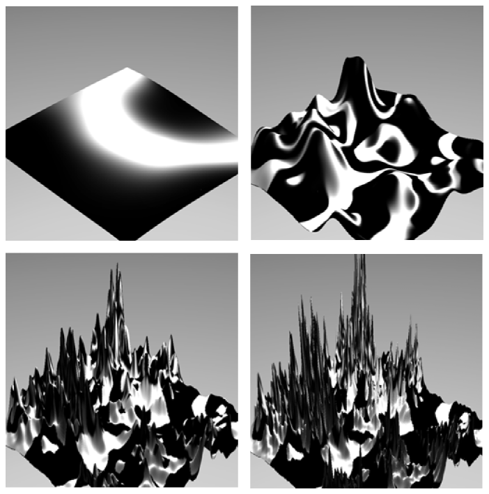
Figure 2: Evolution of scalar fields $\phi$ and $\Phi$ during the process of self-reproduction of the universe. The height of the distribution shows the value of the field $\phi$ which drives inflation. The surface is painted black in those parts of the universe where the scalar field $\Phi$ is in the first minimum of its effective potential, and white where it is in the second minimum. Laws of low-energy physics are different in the regions of different color. The peaks of the “mountains” correspond to places where quantum fluctuations bring the scalar fields back to the Planck density. Each of such places in a certain sense can be considered as a beginning of a new Big Bang.

In the beginning of the process the whole inflationary domain is black, and the distribution of both fields is very homogeneous. Then the domain became exponentially large (but it has the same size in comoving coordinates, as shown in Fig. 2). Each peak of the mountains corresponds to nearly Planckian density and can be interpreted as a beginning of a new “Big Bang.” The laws of physics are rapidly changing there, but they become fixed in the parts of the universe where the field $\phi$ becomes small. These parts correspond to valleys in Fig. 2. Thus quantum fluctuations of the scalar fields divide the universe into exponentially large domains with different laws of low-energy physics, and with different values of energy density.

If this scenario is correct, then physics alone cannot provide a complete explanation for all properties of our part of the universe. The same physical theory may yield large parts of the universe that have diverse properties. According to this scenario, we find ourselves inside a four-dimensional domain with our kind of physical laws not because domains with different dimensionality and with alternate properties are impossible or improbable, but simply because our kind of life cannot exist in other domains.

The fact that inflation may happen in a different manner in different parts of the universe was recognized at the very early stages of development of inflationary theory, which allowed us to justify the use of anthropic principle in inflationary cosmology Linde:1984je . Eternal inflation makes it possible to go even further: It implies that even if the universe started in a single domain with well defined initial conditions, the process of eternal inflation will divide it into infinitely many exponentially large domains that have different laws of low-energy physics Eternal ; LLM . Among all of these domains, we can live and make observations only in those that are compatible with our existence.

Eternal inflation scenario was extensively studied during the last 20 years. I should mention, in particular, the discovery of the topological eternal inflation TopInf , calculation of the fractal dimension of the universe Aryal:1987vn ; LLM , and development of various methods describing statistical/probabilistic aspects of the self-reproducing universe, see LLM ; Garcia-Bellido:1993wn ; Vilenkin:1995yd ; Tegmark:2004qd and references therein. This scenario may have especially interesting implications in the context of string theory, which allows exponentially large number of different de Sitter vacuum states book ; landscape ; BP ; Douglas , see Sect. XIII.

VI Creation of matter after inflation: reheating and preheating

The theory of reheating of the universe after inflation is the most important application of the quantum theory of particle creation, since almost all matter constituting the universe was created during this process.

At the stage of inflation all energy is concentrated in a classical slowly moving inflaton field $\phi$. Soon after the end of inflation this field begins to oscillate near the minimum of its effective potential. Eventually it produces many elementary particles, they interact with each other and come to a state of thermal equilibrium with some temperature $T_{r}$.

Early discussions of reheating of the universe after inflation oldtheory were based on the idea that the homogeneous inflaton field can be represented as a collection of the particles of the field $\phi$. Each of these particles decayed independently. This process can be studied by the usual perturbative approach to particle decay. Typically, it takes thousands of oscillations of the inflaton field until it decays into usual elementary particles by this mechanism. More recently, however, it was discovered that coherent field effects such as parametric resonance can lead to the decay of the homogeneous field much faster than would have been predicted by perturbative methods, within few dozen oscillations KLS . These coherent effects produce high energy, nonthermal fluctuations that could have significance for understanding developments in the early universe, such as baryogenesis. This early stage of rapid nonperturbative decay was called ‘preheating.’ In tach it was found that another effect known as tachyonic preheating can lead to even faster decay than parametric resonance. This effect occurs whenever the homogeneous field rolls down a tachyonic ($V^{\prime\prime}<0$) region of its potential. When that occurs, a tachyonic, or spinodal instability leads to exponentially rapid growth of all long wavelength modes with $k^{2}<|V^{\prime\prime}|$. This growth can often drain all of the energy from the homogeneous field within a single oscillation.

We are now in a position to classify the dominant mechanisms by which the homogeneous inflaton field decays in different classes of inflationary models. Even though all of these models, strictly speaking, belong to the general class of chaotic inflation (none of them is based on the theory of thermal initial conditions), one can break them into three classes: small field, or new inflation models New , large field, or chaotic inflation models of the type of the model $m^{2}\phi^{2}/2$ Chaot , and multi-field, or hybrid models Hybrid . This classification is incomplete, but still rather helpful.

In the simplest versions of chaotic inflation, the stage of preheating is generally dominated by parametric resonance, although there are parameter ranges where this can not occur KLS . In tach it was shown that tachyonic preheating dominates the preheating phase in hybrid models of inflation. New inflation in this respect occupies an intermediate position between chaotic inflation and hybrid inflation: If spontaneous symmetry breaking in this scenario is very large, reheating occurs due to parametric resonance and perturbative decay. However, for the models with spontaneous symmetry breaking at or below the GUT scale, $\phi\ll 10^{{-2}}M_{p}$, preheating occurs due to a combination of tachyonic preheating and parametric resonance. The resulting effect is very strong, so that the homogeneous mode of the inflaton field typically decays within few oscillations Desroche:2005yt .

A detailed investigation of preheating usually requires lattice simulations, which can be achieved following latticeold ; latticeeasy . Note that preheating is not the last stage of reheating; it is followed by a period of turbulence thermalization , by a much slower perturbative decay described by the methods developed in oldtheory , and by eventual thermalization.

VII Inflation and observations

Inflation is not just an interesting theory that can resolve many difficult problems of the standard Big Bang cosmology. This theory made several predictions which can be tested by cosmological observations. Here are the most important predictions:

1) The universe must be flat. In most models $\Omega_{total}=1\pm 10^{-4}$.

2) Perturbations of metric produced during inflation are adiabatic.

3) Inflationary perturbations have nearly flat spectrum. In most inflationary models the spectral index $n_{s}=1\pm 0.2$ ($n_{s}=1$ means totally flat).

4) The spectrum of inflationary perturbations should be slightly non-flat. (It is very difficult to construct a model with $n_{s}=1$.)

5) These perturbations are gaussian.

6) Perturbations of metric could be scalar, vector or tensor. Inflation mostly produces scalar perturbations, but it also produces tensor perturbations with nearly flat spectrum, and it does not produce vector perturbations. There are certain relations between the properties of scalar and tensor perturbations produced by inflation.

7) Inflationary perturbations produce specific peaks in the spectrum of CMB radiation. (For a simple pedagogical interpretation of this effect see e.g. Dodelson:2003ip ; a detailed theoretical description can be found in Mukhanov:2003xr .)

It is possible to violate each of these predictions if one makes this theory sufficiently complicated. For example, it is possible to produce vector perturbations of metric in the models where cosmic strings are produced at the end of inflation, which is the case in some versions of hybrid inflation. It is possible to have an open or closed inflationary universe, or even a small periodic inflationary universe, it is possible to have models with nongaussian isocurvature fluctuations with a non-flat spectrum. However, it is very difficult to do so, and most of the inflationary models obey the simple rules given above.

It is not easy to test all of these predictions. The major breakthrough in this direction was achieved due to the recent measurements of the CMB anisotropy. The latest results based on the WMAP experiment, in combination with the Sloan Digital Sky Survey, are consistent with predictions of the simplest inflationary models with adiabatic gaussian perturbations, with $\Omega=1.01\pm 0.02$, and $n_{s}=0.98\pm 0.03$ WMAP ; Tegmark ; Seljak , see Fig. 3.

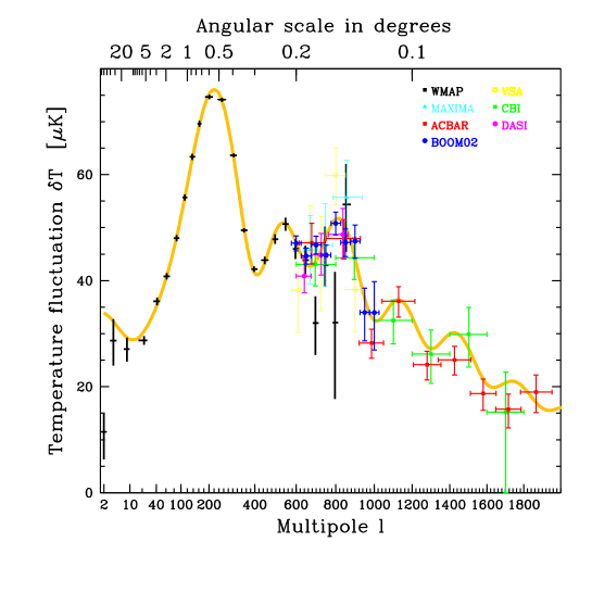
Figure 3: CMB data versus the predictions of one of the simplest inflationary models (thick yellow line), according to Tegmark .

There are still some question marks to be examined, such as an unexpectedly small anisotropy of CMB at large angles WMAP and possible correlations between low multipoles. However, the observational status and interpretation of these effects is rather uncertain Efstathiou:2003wr , and it is quite significant that all proposed explanations of these observations are based on inflationary cosmology, see e.g. Contaldi .

VIII Alternatives to inflation?

Inflationary scenario is very versatile, and now, after 20 years of persistent attempts of many physicists to propose an alternative to inflation, we still do not know any other way to construct a consistent cosmological theory. Indeed, in order to compete with inflation a new theory should make similar predictions and should offer an alternative solution to many difficult cosmological problems. Let us look at these problems before starting a discussion.

1) Homogeneity problem. Before even starting investigation of density perturbations and structure formation, one should explain why the universe is nearly homogeneous on the horizon scale.

2) Isotropy problem. We need to understand why all directions in the universe are similar to each other, why there is no overall rotation of the universe. etc.

3) Horizon problem. This one is closely related to the homogeneity problem. If different parts of the universe have not been in a causal contact when the universe was born, why do they look so similar?

4) Flatness problem. Why $\Omega\approx 1$? Why parallel lines do not intersect?

5) Total entropy problem. The total entropy of the observable part of the universe is greater than $10^{87}$. Where did this huge number come from? Note that the lifetime of a closed universe filled with hot gas with total entropy $S$ is $S^{2/3}\times 10^{-43}$ seconds book . Thus $S$ must be huge. Why?

6) Total mass problem. The total mass of the observable part of the universe has mass $\sim 10^{60}M_{p}$. Note also that the lifetime of a closed universe filled with nonrelativistic particles of total mass $M$ is ${M\over M_{P}}\times 10^{-43}$ seconds. Thus $M$ must be huge. But why?

7) Structure formation problem. If we manage to explain the homogeneity of the universe, how can we explain the origin of inhomogeneities required for the large scale structure formation?

8) Monopole problem, gravitino problem, etc.

This list is very long. That is why it was not easy to propose any alternative to inflation even before we learned that $\Omega\approx 1$, $n_{s}\approx 1$, and that the perturbations responsible for galaxy formation are mostly adiabatic, in agreement with the predictions of the simplest inflationary models.

Despite this difficulty, there was always a tendency to announce that we have eventually found a good alternative to inflation. This was the ideology of the models of structure formation due to topological defects, or textures, which were often described as competitors to inflation, see e.g. SperTur . However, it was clear from the very beginning that these theories at best could solve only one problem (structure formation) out of 8 problems mentioned above. Therefore the true question was not whether one can replace inflation by the theory of cosmic strings/textures, but whether inflation with cosmic strings/textures is better than inflation without cosmic strings/textures. Recent observational data favor the simplest version of inflationary theory, without topological defects, or with an extremely small (few percent) admixture of the effects due to cosmic strings.

A similar situation emerged with the introduction of the ekpyrotic scenario KOST . In the original version of this theory it was claimed that this scenario can solve all cosmological problems without using the stage of inflation, i.e. without a prolonged stage of an accelerated expansion of the universe, which was called in KOST “superluminal expansion.” However, this original idea did not work KKL ; KKLTS , and the idea to avoid “superluminal expansion” was abandoned by the authors of KOST . A more recent version of this scenario, the cyclic scenario cyclic , uses an infinite number of periods of “superluminal expansion”, i.e. inflation, in order to solve the major cosmological problems. In this sense, the cyclic scenario is not a true alternative to inflationary scenario, but its rather peculiar version. The main difference between the usual inflation and the cyclic inflation, just as in the case of topological defects and textures, is the mechanism of generation of density perturbations. However, since the theory of density perturbations in cyclic inflation requires a solution of the cosmological singularity problem Liu:2002ft ; Horowitz:2002mw , it is difficult to say anything definite about it. The latest attempts to do so (despite our inability to address the singularity problem) indicate that the spectrum of metric perturbations produced in the cyclic scenario is incompatible with observations Creminelli:2004jg ; Bozza:2005wn .

Thus at the moment it is hard to see any real alternative to inflationary cosmology; instead of a competition between inflation and other ideas, we witness a competition between many different models of inflationary theory.

This competition goes in several different directions. First of all, we must try to implement inflation in realistic theories of fundamental interactions. But what do we mean by ‘realistic?’ Here we have an interesting and even somewhat paradoxical situation. In the absence of a direct confirmation of M/string theory and supergravity by high energy physics experiments (which may change when we start receiving data from the LHC), the definition of what is realistic becomes increasingly dependent on cosmology and the results of the cosmological observations. In particular, one may argue that those versions of the theory of all fundamental interactions that cannot describe inflation and the present stage of acceleration of the universe are disfavored by observations.

On the other hand, not every theory which can lead to inflation does it in an equally good way. Many inflationary models have been already ruled out be observations. This happened long ago with such models as extended inflation extended and the simplest versions of “natural inflation” natural . Recent data from WMAP and SDSS almost ruled out a particular version of chaotic inflation with $V(\phi)\sim\phi^{4}$ WMAP ; Tegmark .

However, observations test only the last stages of inflation. In particular, they do not say anything about the properties of the inflaton potential at $V(\phi)\gtrsim 10^{-10}M_{p}^{4}$. Thus there may exist many different models which describe all observational data equally well. In order to compare such models, one should not only compare their predictions with the results of the cosmological observations, but also carefully examine whether these models are internally consistent and whether it is possible to solve the problem of initial conditions for inflation in these models. One should also try to find out the best way to implement inflationary scenario in the context of realistic models of all fundamental interactions, including the models based on supergravity and string theory.

IX Shift symmetry and chaotic inflation in supergravity

Most of the existing inflationary models are based on the idea of chaotic initial conditions, which is the trademark of the chaotic inflation scenario. In the simplest versions of chaotic inflation scenario with the potentials $V\sim\phi^{n}$, the process of inflation occurs at $\phi>1$, in Planck units. Meanwhile, there are many other models where inflation may occur at $\phi\ll 1$.

There are several reasons why this difference may be important. First of all, some authors argue that the generic expression for the effective potential can be cast in the form

$$V(\phi)=V_{0}+\alpha\phi+{m^{2}\over 2}\phi^{2}+{\beta\over 3}\phi^{3}+{\lambda\over 4}\phi^{4}+\sum_{n}\lambda_{n}{\phi^{4+n}\over{M_{p}}^{n}}\,,$$ (21)

and then they assume that generically $\lambda_{n}=O(1)$, see e.g. Eq. (128) in LythRiotto . If this assumption were correct, one would have little control over the behavior of $V(\phi)$ at $\phi>M_{p}$.

Here we have written $M_{p}$ explicitly, to expose the implicit assumption made in LythRiotto . Why do we write $M_{p}$ in the denominator, instead of $1000M_{p}$? An intuitive reason is that quantum gravity is non-renormalizable, so one should introduce a cut-off at momenta $k\sim M_{p}$. This is a reasonable assumption, but it does not imply validity of Eq. (21). Indeed, the constant part of the scalar field appears in the gravitational diagrams not directly, but only via its effective potential $V(\phi)$ and the masses of particles interacting with the scalar field $\phi$. As a result, the terms induced by quantum gravity effects are suppressed not by factors ${\phi^{n}\over{M_{p}}^{n}}$, but by factors $V\over{M_{p}}^{4}$ and $m^{2}(\phi)\over{M_{p}}^{2}$ book . Consequently, quantum gravity corrections to $V(\phi)$ become large not at $\phi>M_{p}$, as one could infer from (21), but only at super-Planckian energy density, or for super-Planckian masses. This justifies our use of the simplest chaotic inflation models.

The simplest way to understand this argument is to consider again the case where the potential of the field $\phi$ is a constant, $V=V_{0}$. Then the theory has a shift symmetry, $\phi\to\phi+c$. This symmetry is not broken by perturbative quantum gravity corrections, so no such terms as $\sum_{n}\lambda_{n}{\phi^{4+n}\over{M_{p}}^{n}}$ are generated. This symmetry may be broken by nonperturbative quantum gravity effects (wormholes? virtual black holes?), but such effects, even if they exist, can be made exponentially small Kallosh:1995hi .

The idea of shift symmetry appears to be very fruitful in application to inflation; we will return to it many times in this paper. However, in some cases the scalar field $\phi$ itself may have physical (geometric) meaning, which may constrain the possible values of the fields during inflation. The most important example is given by $N=1$ supergravity.

The effective potential of the complex scalar field $\Phi$ in supergravity is given by the well-known expression (in units $M_{p}=1$):

$$V=e^{K}\left[K_{\Phi\bar{\Phi}}^{-1}\,|D_{\Phi}W|^{2}-3|W|^{2}\right].$$ (22)

Here $W(\Phi)$ is the superpotential, $\Phi$ denotes the scalar component of the superfield $\Phi$; $D_{\Phi}W={\partial W\over\partial\Phi}+{\partial K\over\partial\Phi}W$. The kinetic term of the scalar field is given by $K_{\Phi\bar{\Phi}}\,\partial_{\mu}\Phi\partial_{\mu}\bar{\Phi}$. The standard textbook choice of the Kähler potential corresponding to the canonically normalized fields $\Phi$ and $\bar{\Phi}$ is $K=\Phi\bar{\Phi}$, so that $K_{\Phi\bar{\Phi}}=1$.

This immediately reveals a problem: At $\Phi>1$ the potential is extremely steep. It blows up as $e^{|\Phi|^{2}}$, which makes it very difficult to realize chaotic inflation in supergravity at $\phi\equiv\sqrt{2}|\Phi|>1$. Moreover, the problem persists even at small $\phi$. If, for example, one considers the simplest case when there are many other scalar fields in the theory and the superpotential does not depend on the inflaton field $\phi$, then Eq. (22) implies that at $\phi\ll 1$ the effective mass of the inflaton field is $m^{2}_{\phi}=3H^{2}$. This violates the condition $m^{2}_{\phi}\ll H^{2}$ required for successful slow-roll inflation (so-called $\eta$-problem).

The major progress in SUGRA inflation during the last decade was achieved in the context of the models of the hybrid inflation type, where inflation may occur at $\phi\ll 1$. Among the best models are the F-term inflation, where different contributions to the effective mass term $m^{2}_{\phi}$ cancel F , and D-term inflation D , where the dangerous term $e^{K}$ does not affect the potential in the inflaton direction. A detailed discussion of various versions of hybrid inflation in supersymmetric theories can be found in LythRiotto . A recent version of this scenario, P-term inflation, which unifies F-term and D-term models, was proposed in pterm .

However, hybrid inflation occurs only on a relatively small energy scale, and many of its versions do not lead to eternal inflation. Therefore it would be nice to obtain inflation in a context of a more general class of supergravity models.

This goal seemed very difficult to achieve; it took almost 20 years to find a natural realization of chaotic inflation model in supergravity. Kawasaki, Yamaguchi and Yanagida suggested to take the Kähler potential

$$K={1\over 2}(\Phi+\bar{\Phi})^{2}+X\bar{X}$$ (23)

of the fields $\Phi$ and $X$, with the superpotential $m\Phi X$ jap .

At the first glance, this Kähler potential may seem somewhat unusual. However, it can be obtained from the standard Kähler potential $K=\Phi\bar{\Phi}+X\bar{X}$ by adding terms $\Phi^{2}/2+\bar{\Phi}^{2}/2$, which do not give any contribution to the kinetic term of the scalar fields $K_{\Phi\bar{\Phi}}\,\partial_{\mu}\Phi\partial_{\mu}\bar{\Phi}$. In other words, the new Kähler potential, just as the old one, leads to canonical kinetic terms for the fields $\Phi$ and $X$, so it is as simple and legitimate as the standard textbook Kähler potential. However, instead of the U(1) symmetry with respect to rotation of the field $\Phi$ in the complex plane, the new Kähler potential has a shift symmetry; it does not depend on the imaginary part of the field $\Phi$. The shift symmetry is broken only by the superpotential.

This leads to a profound change of the potential (22): the dangerous term $e^{K}$ continues growing exponentially in the direction $(\Phi+\bar{\Phi})$, but it remains constant in the direction $(\Phi-\bar{\Phi})$. Decomposing the complex field $\Phi$ into two real scalar fields, $\Phi={1\over\sqrt{2}}(\eta+i\phi)$, one can find the resulting potential $V(\phi,\eta,X)$ for $\eta,|X|\ll 1$:

$$V={m^{2}\over 2}\phi^{2}(1+\eta^{2})+m^{2}|X|^{2}.$$ (24)

This potential has a deep valley, with a minimum at $\eta=X=0$. Therefore the fields $\eta$ and $X$ rapidly fall down towards $\eta=X=0$, after which the potential for the field $\phi$ becomes $V={m^{2}\over 2}\phi^{2}$. This provides a very simple realization of eternal chaotic inflation scenario in supergravity jap . This model can be extended to include theories with different power-law potentials, or models where inflation begins as in the simplest versions of chaotic inflation scenario, but ends as in new or hybrid inflation, see e.g. Yamaguchi:2001pw ; Yok .

It is amazing that for almost 20 years nothing but inertia was keeping us from using the version of the supergravity which was free from the famous $\eta$ problem. As we will see shortly, the situation with inflation in string theory is very similar, and may have a similar resolution.

X Towards Inflation in String Theory

X.1 de Sitter vacua in string theory

For a long time, it seemed rather difficult to obtain inflation in M/string theory. The main problem here was the stability of compactification of internal dimensions. For example, ignoring non-perturbative effects to be discussed below, a typical effective potential of the effective 4d theory obtained by compactification in string theory of type IIB can be represented in the following form:

$$V(\varphi,\rho,\phi)\sim e^{\sqrt{2}\varphi-\sqrt{6}\rho}\ \tilde{V}(\phi)$$ (25)

Here $\varphi$ and $\rho$ are canonically normalized fields representing the dilaton field and the volume of the compactified space; $\phi$ stays for all other fields, including the inflaton field.

If $\varphi$ and $\rho$ were constant, then the potential $\tilde{V}(\phi)$ could drive inflation. However, this does not happen because of the steep exponent $e^{\sqrt{2}\varphi-\sqrt{6}\rho}$, which rapidly pushes the dilaton field $\varphi$ to $-\infty$, and the volume modulus $\rho$ to $+\infty$. As a result, the radius of compactification becomes infinite; instead of inflating, 4d space decompactifies and becomes 10d.

Thus in order to describe inflation one should first learn how to stabilize the dilaton and the volume modulus. The dilaton stabilization was achieved in GKP . The most difficult problem was to stabilize the volume. The solution of this problem was found in KKLT (KKLT construction). It consists of two steps.

First of all, due to a combination of effects related to warped geometry of the compactified space and nonperturbative effects calculated directly in 4d (instead of being obtained by compactification), it was possible to obtain a supersymmetric AdS minimum of the effective potential for $\rho$. In the original version of the KKLT scenario, it was done in the theory with the Kähler potential

$$K=-3\log(\rho+\bar{\rho}),$$ (26)

and with the nonperturbative superpotential of the form

$$W=W_{0}+Ae^{-a\rho},$$ (27)

with $a=2\pi/N$. The corresponding effective potential for the complex field $\rho=\sigma+i\alpha$ had a minimum at finite, moderately large values of the volume modulus field $\sigma_{0}$, which fixed the volume modulus in a state with a negative vacuum energy. Then an anti-${D3}$ brane with the positive energy $\sim\sigma^{-2}$ was added. This addition uplifted the minimum of the potential to the state with a positive vacuum energy, see Fig. 4.

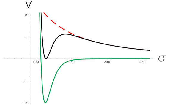
Figure 4: KKLT potential as a function of $\sigma={\rm Re}\,\rho$. Thin green line corresponds to AdS stabilized potential for $W_{0}=-10^{{-4}}$, $A=1$, $a=0.1$. Dashed line shows the additional term, which appears either due to the contribution of a $\overline{D3}$ brane or of a D7 brane. Thick black line shows the resulting potential with a very small but positive value of $V$ in the minimum. All potentials are shown multiplied by $10^{15}$.

Instead of adding an anti-${D3}$ brane, which explicitly breaks supersymmetry, one can add a D7 brane with fluxes. This results in the appearance of a D-term which has a similar dependence on $\rho$, but leads to spontaneous supersymmetry breaking Burgess:2003ic . In either case, one ends up with a metastable dS state which can decay by tunneling and formation of bubbles of 10d space with vanishing vacuum energy density. The decay rate is extremely small KKLT , so for all practical purposes, one obtains an exponentially expanding de Sitter space with the stabilized volume of the internal space.

X.2 Inflation in string theory

There are two different versions of string inflation. In the first version, which we will call modular inflation, the inflaton field is associated with one of the moduli, the scalar fields which are already present in the KKLT construction. In the second version, the inflaton is related to the distance between branes moving in the compactified space. (This scenario should not be confused with inflation in the brane world scenario Arkani-Hamed:1998rs ; Randall:1999ee . This is a separate interesting subject, which we are not going to discuss in this paper.)

X.2.1 Modular inflation

An example of the KKLT-based modular inflation is provided by the racetrack inflation model of Ref. Blanco-Pillado:2004ns . It uses a slightly more complicated superpotential

$$W=W_{0}+Ae^{-a\rho}+Be^{-b\rho}.$$ (28)

The potential of this theory has a saddle point as a function of the real and the complex part of the volume modulus: It has a local minimum in the direction $\rm Re\,\rho$, which is simultaneously a very flat maximum with respect to $\rm Im\,\rho$. Inflation occurs during a slow rolling of the field $\rm Im\,\rho$ away from this maximum (i.e. from the saddle point). The existence of this regime requires a significant fine-tuning of parameters of the superpotential. However, in the context of the string landscape scenario describing from $10^{100}$ to $10^{1000}$ different vacua (see below), this may not be such a big issue. A nice feature of this model is that it does not require adding any new branes to the original KKLT scenario, i.e. it is rather economical. Another attractive feature of this model is the existence of the regime of eternal inflation near the saddle point.

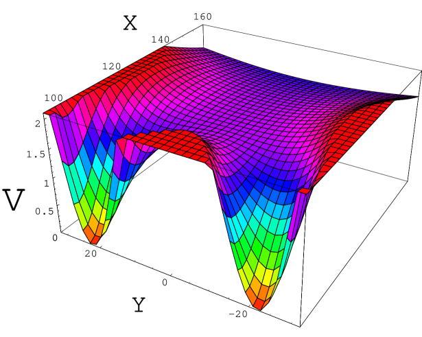
Figure 5: Plot for the potential in the racetrack model (rescaled by $10^{16}$). Here X stays for $\sigma={\rm Re}\,\rho$ and Y stays for $\alpha={\rm Im}\,\rho$. Inflation begins in a vicinity of the saddle point at $X_{\rm saddle}=123.22$, $Y_{\rm saddle}=0$. Units are $M_{p}=1$.

X.2.2 Brane inflation and shift symmetry

During the last few years there were many suggestions how to obtain hybrid inflation in string theory by considering motion of branes in the compactified space, see Dvali:1998pa ; Quevedo and references therein. The main problem of all of these models was the absence of stabilization of the compactified space. Once this problem was solved for dS space KKLT , one could try to revisit these models and develop models of brane inflation compatible with the volume stabilization.

The first idea KKLMMT was to consider a pair of D3 and anti-D3 branes in the warped geometry studied in KKLT . The role of the inflaton field $\phi$ could be played by the interbrane separation. A description of this situation in terms of the effective 4d supergravity involved Kähler potential

$$K=-3\log(\rho+\bar{\rho}-k(\phi,\bar{\phi})),$$ (29)

where the function $k(\phi,\bar{\phi})$ for the inflaton field $\phi$, at small $\phi$, was taken in the simplest form $k(\phi,\bar{\phi})=\phi\bar{\phi}$. If one makes the simplest assumption that the superpotential does not depend on $\phi$, then the $\phi$ dependence of the potential (22) comes from the term $e^{K}=(\rho+\bar{\rho}-\phi\bar{\phi})^{-3}$. Expanding this term near the stabilization point $\rho=\rho_{0}$, one finds that the inflaton field has a mass $m^{2}_{\phi}=2H^{2}$. Just like the similar relation $m^{2}_{\phi}=3H^{2}$ in the simplest models of supergravity, this is not what we want for inflation.

One way to solve this problem is to consider $\phi$-dependent superpotentials. By doing so, one may fine-tune $m^{2}_{\phi}$ to be $O(10^{-2})H^{2}$ in a vicinity of the point where inflation occurs KKLMMT . Whereas fine-tuning is certainly undesirable, in the context of string cosmology it may not be a serious drawback. Indeed, if there exist many realizations of string theory Douglas , then one might argue that all realizations not leading to inflation can be discarded, because they do not describe a universe in which we could live. Meanwhile, those non-generic realizations, which lead to eternal inflation, describe inflationary universes with an indefinitely large and ever-growing volume of inflationary domains. This makes the issue of fine-tuning less problematic. A more detailed investigation of this issue can be found in Buchel:2003qj .

Can we avoid fine-tuning altogether? One of the possible ideas is to find theories with some kind of shift symmetry. Another possibility is to construct something like D-term inflation, where the flatness of the potential is not spoiled by the term $e^{K}$. Both of these ideas were explored in Ref. Hsu:2003cy based on the model of D3/D7 inflation in string theory renata . In this model the Kähler potential is given by

$$K=-3\log(\rho+\bar{\rho})-{1\over 2}(\phi-\bar{\phi})^{2},$$ (30)

and superpotential depends only on $\rho$. The role of the inflaton field is played by the field $s={\rm Re}\,\phi$, which represents the distance between the D3 and D7 branes. The shift symmetry $s\to s+c$ in this model is related to the requirement of unbroken supersymmetry of branes in a BPS state.

The effective potential with respect to the field $\rho$ in this model coincides with the KKLT potential KKLT ; Burgess:2003ic . The potential is exactly flat in the direction of the inflaton field $s$, see Fig. 6, until one adds a hypermultiplet of other fields $\phi_{\pm}$, which break this flatness due to quantum corrections and produce a logarithmic potential for the field $s$. The resulting potential with respect to the fields $s$ and $\phi_{\pm}$ is very similar to the potential of D-term hybrid inflation D .

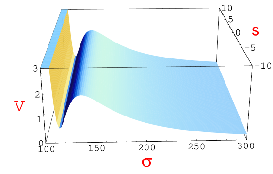
Figure 6: Inflationary potential as a function of the compactification modulus $\sigma$ and the inflaton field $s$. This potential is exactly flat in the inflaton direction due to shift symmetry, which is violated only by radiative corrections.

During inflation, $\phi_{\pm}=0$, and the field $s$ slowly rolls down to its smaller values. When it becomes sufficiently small, the theory becomes unstable with respect to generation of the field $\phi_{+}$, see Fig. 7. The fields $s$ and $\phi_{+}$ roll down to the KKLT minimum, and inflation ends.

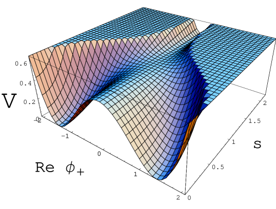
Figure 7: Inflationary potential as a function of the inflaton field $s$ and ${\rm Re}\,\phi_{+}$. In the beginning, the field $s$ rolls along the valley $\phi_{+}=0$, and then it falls down to the KKLT minimum.

One may wonder whether the shift symmetry is just a condition which we want to impose on the theory in order to get inflation Tye , or an unavoidable property of the theory, which remains valid even after the KKLT volume stabilization. The answer to this question appears to be model-dependent. It was shown in Angelantonj:2003up ; kalrecent that in a certain class of models, including D3/D7 models renata ; Hsu:2003cy ; Koyama:2003yc , the shift symmetry of the effective 4d theory is not an assumption but an unambiguous consequence of the underlying mathematical structure of the theory. This may allow us to obtain a natural realization of inflation in string theory. For the latest developments in D3/D7 inflation see Dasgupta:2004dw ; Chen:2005ae ; KLupdate .

All inflationary models discussed above were formulated in the context of Type IIB string theory with the KKLT stabilization. A discussion of the possibility to obtain inflation in the heterotic string theory with stable compactification can be found in Buchbinder:2004nt ; Becker:2005sg .

Finally, we should mention that making the effective potential flat is not the only way to achieve inflation. There are some models with nontrivial kinetic terms where inflation may occur even without any potential kinfl . One may also consider models with steep potentials but with anomalously large kinetic terms for the scalar fields see e.g. Dim . In application to string theory, such models, called ‘DBI inflation,’ were developed in Silverstein:2003hf .

XI Scale of inflation, scale of SUSY breaking and the gravitino mass

So far, we did not discuss relation of the new class of models with particle phenomenology. This relation is rather unexpected and may impose strong constraints either on particle phenomenology or on inflationary models: Recently it was shown that the Hubble constant and the inflaton mass in the simplest models based on the KKLT mechanism with the superpotential (27) are always smaller than the gravitino mass Kallosh:2004yh ,

$$H\lesssim m_{{3/2}}\ .$$ (31)

The reason for this constraint is that adding a large vacuum energy density to the KKLT potential may destabilize it, see Fig. 8.

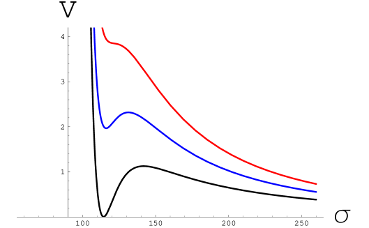
Figure 8: The lowest curve with dS minimum is the one from the KKLT model. The height of the barrier in this potential is of the order $m_{3/2}^{2}$. The second line shows the $\sigma$-dependence of the D3/D7 inflationary potential with the term $V_{\rm infl}={V(s,\phi_{\pm})\over\sigma^{3}}$ added to the KKLT potential; it originates from fluxes on D7 brane. The top curve shows that when the inflationary potential becomes too large, the barrier disappears, and the internal space decompactifies. This explains the origin of the constraint $H\lesssim m_{3/2}$. This constraint appears in a broad class of inflationary models based on the simplest KKLT potential.

Since in the slow-roll models the inflaton mass must be much smaller than $H$, its mass must be much smaller than $m_{{3/2}}$. Therefore if one insists on the standard SUSY phenomenology assuming that the gravitino mass is smaller than $O(1)$ TeV, one will need to find realistic particle physics model where the nonperturbative string theory dynamics occurs at the LHC scale (!!!), and inflation occurs at least 30 orders of magnitude below the Planck energy density. Such models are possible, but their parameters should be substantially different from the parameters used in all presently existing models of string theory inflation.

There are several different ways to address this problem. First of all, one may try to construct realistic particle physics models with superheavy gravitinos DeWolfe:2002nn ; Arkani-Hamed:2004fb . Another possibility is to consider models with the racetrack superpotential (28) and find such parameters that the minimum of the potential even before the uplifting will occur at vanishingly small energy density. This goal was achieved in Kallosh:2004yh .

Figure 9: The potential in the theory (28) for $A=1,\ B=-5,\ a=2\pi/100,\ b=2\pi/50,\ W_{0}=-0.05$. A Minkowski minimum at $V=0$ stabilizes the volume at $\sigma_{0}\approx 37$. AdS vacuum at $V<0$ occurs at $\sigma_{0}\sim 66$. There is a barrier protecting the Minkowski minimum, with the height $V_{{\rm B}}\sim 5\times 10^{-9}$, in units of the Planck energy density. The height of the barrier is not correlated with the gravitino mass, which vanishes if the system is trapped in Minkowski vacuum.

An intriguing property of the new version of the KKLT construction is that the minimum of the potential prior to the uplifting corresponds to a supersymmetric Minkowski vacuum. The gravitino mass in this minimum (and the magnitude of SUSY breaking there) can be vanishingly small as compared to all other parameters of the model, and the constraint $H\lesssim m_{{3/2}}$ disappears. Anywhere outside this minimum the gravitino mass and the magnitude of SUSY breaking is extremely large. This means that the Minkowski minimum shown in Fig. 9 is a point of enhanced symmetry, which is a trapping point for the motion of the moduli fields, in accordance with Kofman:2004yc . This fact may increase the probability that among all possible minima in the string theory landscape, the minimum with a low-scale SUSY breaking is dynamically preferred.

The original KKLT model with the potential shown by the black line in Fig. 4, and its new version with the potential shown in Fig. 9, represent the two presently available models of dark energy based on string theory. In both cases the universe experiences constant acceleration determined by the small positive vacuum energy in the minimum of the potential. In both cases, these vacuum states are expected to be metastable, with an extremely long lifetime. These states may decay by forming expanding bubble of a new phase. It would be very hard to detect such a bubble and even harder to report the results of the observations, since the bubble walls move with the speed approaching the speed of light, so an observer would see the bubble wall at the moment when it hits him.

The difference between these two versions is that the interior of the bubble in the simplest version of the KKLT scenario represents a 10D Minkowski space, whereas an interior of the bubble in its modified version shown in Fig. 9 will correspond to a very rapidly collapsing open universe with a negative energy density.

The only good thing about this grim picture is that in an eternally existing self-reproducing universe there will always remain some parts of space where somebody else will enjoy life.

XII Initial conditions for the low-scale inflation and topology of the universe

One of the advantages of the simplest chaotic inflation scenario is that inflation may begin in the universe immediately after its creation at the largest possible energy density $M_{p}^{4}$, of a smallest possible size (Planck length), with the smallest possible mass $M\sim M_{p}$ and with the smallest possible entropy $S=O(1)$. This provides a true solution to the flatness, horizon, homogeneity, mass and entropy problems book .

Meanwhile, in the new inflation scenario, inflation occurs on the mass scale 3 orders of magnitude below $M_{p}$, when the total size of the universe was very large. If, for example, the universe is closed, its total mass at the beginning of new inflation must be greater than $10^{6}M_{p}$, and its total entropy must be greater than $10^{9}$. In other words, in order to explain why the entropy of the universe at present is greater than $10^{87}$ one should assume that it was extremely large from the very beginning. This does not look like a real solution of the entropy problem. A similar problem exists for many of the models advocated in Lyth:2003kp ; Boubekeur:2005zm . Finally, in cyclic inflation, the process of exponential expansion of the universe occurs only if the total mass of the universe is greater than its present mass $M\sim 10^{60}M_{p}$ and its total entropy is greater than $10^{87}$. This scenario does not solve the flatness, mass and entropy problems.

Is it at all possible to solve the problem of initial conditions for the low scale inflation? The answer to this question appears to be positive though perhaps somewhat unexpected: One should consider a compact flat or open universe with nontrivial topology (usual flat or open universes are infinite). The universe may initially look like a nearly homogeneous torus of a Planckian size containing just one or two photons or gravitons. It can be shown that such a universe continues expanding and remains homogeneous until the onset of inflation, even if inflation occurs only at a very low scale ZelStar ; chaotmix ; topol4 ; Coule ; Linde:2004nz .

Consider for simplicity the flat compact universe having the topology of a torus, $S_{1}^{3}$,

$$ds^{2}=dt^{2}-a_{i}^{2}(t)\,dx_{i}^{2}$$ (32)

with identification $x_{i}+1=x_{i}$ for each of the three dimensions. Consider for simplicity the case $a_{1}=a_{2}=a_{3}=a(t)$. In this case the curvature of the universe and the Einstein equations written in terms of $a(t)$ will be the same as in the infinite flat Friedmann universe with metric $ds^{2}=dt^{2}-a^{2}(t)\,d{\bf x^{2}}$. In our notation, the scale factor $a(t)$ is equal to the size of the universe in Planck units $M_{p}^{{-1}}=1$.

Let us assume, that at the Planck time $t_{p}\sim M_{p}^{-1}=1$ the universe was radiation dominated, $V\ll T^{4}=O(1)$. Let us also assume that at the Planck time the total size of the box was Planckian, $a(t_{p})=O(1)$. In such case the whole universe initially contained only $O(1)$ relativistic particles such as photons or gravitons, so that the total entropy of the whole universe was O(1).

The size of the universe dominated by relativistic particles was growing as $a(t)\sim\sqrt{t}$, whereas the mean free path of the gravitons was growing as $H^{-1}\sim t$. If the initial size of the universe was $O(1)$, then at the time $t\gg 1$ each particle (or a gravitational perturbation of metric) within one cosmological time would run all over the torus many times, appearing in all of its parts with nearly equal probability. This effect, called “chaotic mixing,” should lead to a rapid homogenization of the universe chaotmix ; topol4 . Note, that to achieve a modest degree of homogeneity required for inflation to start when the density of ordinary matter drops down, we do not even need chaotic mixing. Indeed, density perturbations do not grow in a universe dominated by ultrarelativistic particles if the size of the universe is smaller than $H^{-1}$. This is exactly what happens in our model. Therefore the universe should remain relatively homogeneous until the thermal energy density drops below $V$ and inflation begins.

Thus we see that in this scenario, just as in the simplest chaotic inflation scenario, inflation begins if we had a sufficiently homogeneous domain of a smallest possible size (Planck scale), with the smallest possible mass (Planck mass), and with the total entropy O(1). The only additional requirement is that this domain should have identified sides, in order to make a flat or open universe compact. We see no reason to expect that the probability of formation of such domains is strongly suppressed.

One can come to a similar conclusion from a completely different point of view. Investigation of the quantum creation of a closed or an infinite open inflationary universe with a small value of the vacuum energy shows that this process is forbidden at the classical level, and therefore it occurs only due to tunneling. As a result, the probability of this process is exponentially suppressed Linde:1983mx ; Vilenkin:1984wp ; Open . Meanwhile, creation of the flat or open universe is possible without any need for the tunneling, and therefore there is no exponential suppression for the probability of quantum creation of a topologically nontrivial compact flat or open inflationary universe ZelStar ; Coule ; Linde:2004nz ; KLS2005 .

These results suggest that if inflation can occur only much below the Planck density, then the topologically nontrivial flat or open universes should be much more probable than the standard Friedmann universes described in every textbook on cosmology.

Until now, we discussed creation of compact universes which have approximately equal size in all directions. If at the Planck time our universe was of a Planck size in some directions, but it was much larger in some other directions, then it consisted of many causally disconnected Planck size regions. This results in a particular version of the horizon/homogeneity problem: The probability that the universe was homogeneous in all of these causally disconnected regions should be exponentially small KLS2005 .

In application to the initial conditions in the 10D universe described by string theory, this suggests that it is more natural to start with the universe which would have similar initial size in all 9 spatial directions. In terms of the KKLT potential, this implies that the initial value of the volume modulus $\sigma$ should be very small, so that $V(\sigma)=O(1)$. But then the field $\sigma$ will rapidly fall down. It can easily roll over the very law KKLT barrier, and continue moving to infinitely large $\sigma$.

One of the recent attempts to solve this problem was based on the dynamical slow-down of the field $\sigma$ in the universe filled with radiation Brustein:2004jp . But this mechanism typically works only if the initial value of the effective potential is several orders of magnitude smaller than O(1).

It is not quite clear whether this is a real problem because those parts of the universe which start at large $V(\sigma)$, become ten-dimensional, so we cannot live there. We will live in the parts of the universe which started at smaller $V(\sigma)$, even if it may seem improbable from the point of view of initial conditions. This is similar to the fact that we live at the 2D surface of a relatively small planet instead of living in the vast but empty interstellar space.

One can also argue LLM that eternal inflation may alleviate some of the problems of the problem of initial conditions for the low-scale inflation. Note, however, that eternal inflation, which naturally occurs in the simplest versions of chaotic inflation, in new inflation, and in the racetrack scenario Blanco-Pillado:2004ns , may not exist in many versions of string theory inflation of the hybrid type, such as the models of KKLMMT ; Hsu:2003cy ; KLupdate . Of course, models of low-scale non-eternal inflation are still much better than the models with no inflation at all, but I do not think that we should settle for the second-best. An indeed we should not, if we are able to combine the slow-roll inflation, which ends in our vacuum, with the eternal inflation in a collection of different metastable dS states in the string theory landscape.

XIII Eternal inflation and the string theory landscape

Even though we are still at the very first stages of implementing inflation in string theory, it is very tempting to speculate about possible generic features and consequences of such a construction.

First of all, KKLT construction shows that the vacuum energy after the volume stabilization is a function of many different parameters in the theory. One may wonder how many different choices do we actually have. There were many attempts to investigate this issue. For example, many years ago it was argued Duff that there are infinitely many $AdS_{4}\times X7$ vacua of D=11 supergravity. An early estimate of the total number of different 4d string vacua gave the number $10^{1500}$ Lerche . At present we are more interested in counting different flux vacua BP ; Douglas , where the possible numbers, depending on specific assumptions, may vary in the range from $10^{20}$ to $10^{1000}$. Some of these vacuum states with positive vacuum energy can be stabilized using the KKLT approach. Each of such states will correspond to a metastable vacuum state. It decays within a cosmologically large time, which is, however, smaller than the ‘recurrence time’ $e^{S(\phi)}$, where $S(\phi)={24\pi^{2}\over V(\phi)}$ is the entropy of dS space with the vacuum energy density $V(\phi)$ KKLT .

But this is not the whole story; old inflation does not describe our world. In addition to these metastable vacuum states, there should exist various slow-roll inflationary solutions, where the properties of the system practically do not change during the cosmological time $H^{-1}$. It might happen that such states, corresponding to flat directions in the string theory landscape, exist not only during inflation in the very early universe, but also at the present stage of the accelerated expansion of the universe. This would simplify obtaining an anthropic solution of the cosmological constant problem along the lines of Linde84 ; BP .

If the slow-roll condition $V^{\prime\prime}\ll V$ is satisfied all the way from one dS minimum of the effective potential to another, then one can show, using stochastic approach to inflation, that the probability to find the field $\phi$ at any of these minima, or at any given point between them, is proportional to $e^{S(\phi)}$. In other words, the relative probability to find the field taking some value $\phi_{1}$ as compared to some other value $\phi_{0}$, is proportional to $e^{\Delta S}=e^{S(\phi_{1})-S(\phi_{0})}$ Open ; KKLT . One may argue, using Euclidean approach, that this simple thermodynamic relation should remain valid for the relative probability to find a given point in any of the metastable dS vacua, even if the trajectory between them does not satisfy the slow-roll condition $m^{2}\ll H^{2}$ HM ; Lee:qc ; Garriga:1997ef ; Dyson:2002pf .

The resulting picture resembles eternal inflation in the old inflation scenario. However, now we have an incredibly large number of false vacuum states, plus some states which may allow slow-roll inflation. Once inflation begins, different parts of the universe start jumping from one of these vacuum states to another, so that the universe becomes divided into indefinitely many regions with all possible laws of low-energy physics corresponding to different 4D vacua of string theory book .

The best inflationary scenario would describe a slow-roll eternal inflation starting at the maximal possible energy density (minimal dS entropy). It would be almost as good to have a low-energy slow-roll eternal inflation. Under certain conditions, such regimes may exist in string theory KKLMMT . Here we are going to discuss a different but equally interesting possibility. Multi-level eternal inflation of the old inflation type, which appears in string theory in the context of the KKLT construction, may be very useful being combined with the slow-roll inflation, even if the slow-roll inflation by itself is not eternal. We will give a particular example, which is based on the ideas developed in Ref. Linde:1987yb .

Suppose we have two noninteracting scalar fields: field $\phi$ with the potential of the old inflation type, and field $s$ with the potential which may lead to a slow-roll inflation. Let us consider the worst case scenario: the slow-roll inflation occurs only on low energy scale, and it is not eternal.

Let us assume that the Hubble constant at the stage of old inflation is much greater than the curvature of the potential which drives the slow-roll inflation. This is a natural assumption, considering huge number of possible dS states, and the presumed smallness of energy scale of the slow-roll inflation. The validity of this assumption is ensured if the shift symmetry with respect to the slow-rolling inflaton field $s$ is preserved in many different string theory vacua. This may be the case in the D3/D7 scenario, where the shift symmetry is related to the isometry of the compactified space but not to the particular values of the fluxes Hsu:2003cy ; kalrecent ; KLupdate . In this case large inflationary fluctuations of the field $s$ will be generated during eternal old inflation. These fluctuations will push the field $s$ from the minimum of its effective potential and will give it different values in different exponentially large parts of the universe. When old inflation ends, there will be many practically homogeneous parts of the universe where the field $s$ will take values corresponding to good initial conditions for a slow-roll inflation.

Thus, the existence of many different dS vacua in string theory leads to the regime of eternal inflation. This regime may help us to solve the problem of initial conditions for the slow-roll inflation even in the models where the slow-roll inflation by itself is not eternal and would occur only on a small energy scale.

- (1) A. A. Starobinsky, “Spectrum Of Relict Gravitational Radiation And The Early State Of The Universe,” JETP Lett. 30, 682 (1979) [Pisma Zh. Eksp. Teor. Fiz. 30, 719 (1979)]; A. A. Starobinsky, “A New Type Of Isotropic Cosmological Models Without Singularity,” Phys. Lett. B 91, 99 (1980).
- (2) V. F. Mukhanov and G. V. Chibisov, “Quantum Fluctuation And ‘Nonsingular’ Universe,” JETP Lett. 33, 532 (1981) [Pisma Zh. Eksp. Teor. Fiz. 33, 549 (1981)].
- (3) A. H. Guth, “The Inflationary Universe: A Possible Solution To The Horizon And Flatness Problems,” Phys. Rev. D 23, 347 (1981).
- (4) D. A. Kirzhnits and A. D. Linde, “Symmetry Behavior In Gauge Theories,” Annals Phys. 101, 195 (1976).
- (5) S. W. Hawking, I. G. Moss and J. M. Stewart, “Bubble Collisions In The Very Early Universe,” Phys. Rev. D 26, 2681 (1982).
- (6) A. H. Guth and E. J. Weinberg, “Could The Universe Have Recovered From A Slow First Order Phase Transition?,” Nucl. Phys. B 212, 321 (1983).
- (7) A. D. Linde, “A New Inflationary Universe Scenario: A Possible Solution Of The Horizon, Flatness, Homogeneity, Isotropy And Primordial Monopole Problems,” Phys. Lett. B 108, 389 (1982); A. D. Linde, “Coleman-Weinberg Theory And A New Inflationary Universe Scenario,” Phys. Lett. B 114, 431 (1982); A. D. Linde, “Temperature Dependence Of Coupling Constants And The Phase Transition In The Coleman-Weinberg Theory,” Phys. Lett. B 116, 340 (1982); A. D. Linde, “Scalar Field Fluctuations In Expanding Universe And The New Inflationary Universe Scenario,” Phys. Lett. B 116, 335 (1982).
- (8) A. Albrecht and P. J. Steinhardt, “Cosmology For Grand Unified Theories With Radiatively Induced Symmetry Breaking,” Phys. Rev. Lett. 48, 1220 (1982).
- (9) S. W. Hawking, “The Development Of Irregularities In A Single Bubble Inflationary Universe,” Phys. Lett. B 115, 295 (1982); A. A. Starobinsky, “Dynamics Of Phase Transition In The New Inflationary Universe Scenario And Generation Of Perturbations,” Phys. Lett. B 117, 175 (1982); A. H. Guth and S. Y. Pi, “Fluctuations In The New Inflationary Universe,” Phys. Rev. Lett. 49, 1110 (1982); J. M. Bardeen, P. J. Steinhardt and M. S. Turner, “Spontaneous Creation Of Almost Scale - Free Density Perturbations In An Inflationary Universe,” Phys. Rev. D 28, 679 (1983).
- (10) V. F. Mukhanov, “Gravitational Instability Of The Universe Filled With A Scalar Field,” JETP Lett. 41, 493 (1985) [Pisma Zh. Eksp. Teor. Fiz. 41, 402 (1985)]; V. F. Mukhanov, H. A. Feldman and R. H. Brandenberger, “Theory Of Cosmological Perturbations,” Phys. Rept. 215, 203 (1992); V. F. Mukhanov, Physical Foundations of Cosmology, Cambridge University Press, to be published.
- (11) A.D. Linde, Particle Physics and Inflationary Cosmology (Harwood, Chur, Switzerland, 1990).
- (12) A. D. Linde, “Chaotic Inflation,” Phys. Lett. B 129, 177 (1983).
- (13) A. D. Dolgov and A. D. Linde, “Baryon Asymmetry In Inflationary Universe,” Phys. Lett. B 116, 329 (1982); L. F. Abbott, E. Farhi and M. B. Wise, “Particle Production In The New Inflationary Cosmology,” Phys. Lett. B 117, 29 (1982).
- (14) L. Kofman, A. D. Linde and A. A. Starobinsky, “Reheating after inflation,” Phys. Rev. Lett. 73, 3195 (1994) [arXiv:hep-th/9405187]; L. Kofman, A. D. Linde and A. A. Starobinsky, “Towards the theory of reheating after inflation,” Phys. Rev. D 56, 3258 (1997) [arXiv:hep-ph/9704452].
- (15) G. N. Felder, J. Garcia-Bellido, P. B. Greene, L. Kofman, A. D. Linde and I. Tkachev, “Dynamics of symmetry breaking and tachyonic preheating,” Phys. Rev. Lett. 87, 011601 (2001) [arXiv:hep-ph/0012142]; G. N. Felder, L. Kofman and A. D. Linde, “Tachyonic instability and dynamics of spontaneous symmetry breaking,” Phys. Rev. D 64, 123517 (2001) [arXiv:hep-th/0106179].
- (16) M. Desroche, G. N. Felder, J. M. Kratochvil and A. Linde, “Preheating in new inflation,” arXiv:hep-th/0501080.
- (17) S. Y. Khlebnikov and I. I. Tkachev, “Classical decay of inflaton,” Phys. Rev. Lett. 77, 219 (1996) [arXiv:hep-ph/9603378]; S. Y. Khlebnikov and I. I. Tkachev, “Resonant decay of Bose condensates,” Phys. Rev. Lett. 79, 1607 (1997) [arXiv:hep-ph/9610477].
- (18) G. N. Felder and I. Tkachev, “LATTICEEASY: A program for lattice simulations of scalar fields in an expanding universe,” arXiv:hep-ph/0011159.
- (19) G. N. Felder and L. Kofman, “The development of equilibrium after preheating,” Phys. Rev. D 63, 103503 (2001) [arXiv:hep-ph/0011160]; R. Micha and I. I. Tkachev, “Turbulent thermalization,” Phys. Rev. D 70, 043538 (2004) [arXiv:hep-ph/0403101].
- (20) B. A. Ovrut and P. J. Steinhardt, “Supersymmetry And Inflation: A New Approach,” Phys. Lett. B 133, 161 (1983); B. A. Ovrut and P. J. Steinhardt, “Inflationary Cosmology And The Mass Hierarchy In Locally Supersymmetric Theories,” Phys. Rev. Lett. 53, 732 (1984); B. A. Ovrut and P. J. Steinhardt, “Locally Supersymmetric Cosmology And The Gauge Hierarchy,” Phys. Rev. D 30, 2061 (1984); B. A. Ovrut and P. J. Steinhardt, “Supersymmetric Inflation, Baryon Asymmetry And The Gravitino Problem,” Phys. Lett. B 147, 263 (1984).
- (21) A. D. Linde, “Primordial Inflation Without Primordial Monopoles,” Phys. Lett. B 132 (1983) 317.
- (22) L. Boubekeur and D. H. Lyth, “Hilltop inflation,” arXiv:hep-ph/0502047.
- (23) A. D. Linde, “Axions in inflationary cosmology,” Phys. Lett. B 259, 38 (1991); A. D. Linde, “Hybrid inflation,” Phys. Rev. D 49, 748 (1994) [astro-ph/9307002].
- (24) A. Vilenkin and L. H. Ford, “Gravitational Effects Upon Cosmological Phase Transitions,” Phys. Rev. D 26, 1231 (1982).
- (25) A. D. Linde, “Scalar Field Fluctuations In Expanding Universe And The New Inflationary Universe Scenario,” Phys. Lett. B 116, 335 (1982).
- (26) D. J. Gross and F. Wilczek, “Ultraviolet Behavior Of Non-Abelian Gauge Theories,” Phys. Rev. Lett. 30, 1343 (1973).
- (27) H. D. Politzer, “Reliable Perturbative Results For Strong Interactions?,” Phys. Rev. Lett. 30, 1346 (1973).
- (28) A.R. Liddle and D. H. Lyth, Cosmological Inflation and Large-Scale Structure, (Cambridge University Press, Cambridge 2000).
- (29) H. V. Peiris et al., “First year Wilkinson Microwave Anisotropy Probe (WMAP) observations: Implications for inflation,” Astrophys. J. Suppl. 148, 213 (2003) [arXiv:astro-ph/0302225].
- (30) M. Tegmark et al. [SDSS Collaboration], “Cosmological parameters from SDSS and WMAP,” Phys. Rev. D 69, 103501 (2004) [arXiv:astro-ph/0310723].
- (31) U. Seljak et al., “Cosmological parameter analysis including SDSS Ly-alpha forest and galaxy bias: Constraints on the primordial spectrum of fluctuations, neutrino mass, and dark energy,” arXiv:astro-ph/0407372.
- (32) K. Sigurdson and A. Cooray, “Cosmic 21-cm Delensing of Microwave Background Polarization and the Minimum Detectable Energy Scale of Inflation,” arXiv:astro-ph/0502549.
- (33) A. D. Linde, “Generation Of Isothermal Density Perturbations In The Inflationary Universe,” Phys. Lett. B 158, 375 (1985); L. A. Kofman and A. D. Linde, “Generation Of Density Perturbations In The Inflationary Cosmology,” Nucl. Phys. B 282 (1987) 555.
- (34) D. H. Lyth and D. Wands, “Generating the curvature perturbation without an inflaton,” Phys. Lett. B 524, 5 (2002) [arXiv:hep-ph/0110002].
- (35) T. Moroi and T. Takahashi, “Effects of cosmological moduli fields on cosmic microwave background,” Phys. Lett. B 522, 215 (2001) [Erratum-ibid. B 539, 303 (2002)] [arXiv:hep-ph/0110096].
- (36) S. Mollerach, “Isocurvature Baryon Perturbations And Inflation,” Phys. Rev. D 42, 313 (1990).
- (37) A. D. Linde and V. Mukhanov, “Nongaussian isocurvature perturbations from inflation,” Phys. Rev. D 56, 535 (1997) [arXiv:astro-ph/9610219].
- (38) G. Dvali, A. Gruzinov and M. Zaldarriaga, “A new mechanism for generating density perturbations from inflation,” Phys. Rev. D 69, 023505 (2004) [arXiv:astro-ph/0303591].
- (39) L. Kofman, “Probing string theory with modulated cosmological fluctuations,” arXiv:astro-ph/0303614; F. Bernardeau, L. Kofman and J. P. Uzan, “Modulated fluctuations from hybrid inflation,” Phys. Rev. D 70, 083004 (2004) [arXiv:astro-ph/0403315].
- (40) P. J. Steinhardt, “Natural Inflation,” In: The Very Early Universe, ed. G.W. Gibbons, S.W. Hawking and S.Siklos, Cambridge University Press, (1983); A. D. Linde, “Nonsingular Regenerating Inflationary Universe,” Cambridge University preprint Print-82-0554 (1982).
- (41) A. Vilenkin, “The Birth Of Inflationary Universes,” Phys. Rev. D 27, 2848 (1983).
- (42) A. D. Linde, “Eternally Existing Self-reproducing Chaotic Inflationary Universe,” Phys. Lett. B 175, 395 (1986); A. S. Goncharov, A. D. Linde and V. F. Mukhanov, “The Global Structure Of The Inflationary Universe,” Int. J. Mod. Phys. A 2, 561 (1987).
- (43) A. D. Linde, D. A. Linde and A. Mezhlumian, “From the Big Bang theory to the theory of a stationary universe,” Phys. Rev. D 49, 1783 (1994) [arXiv:gr-qc/9306035].
- (44) A. Borde, A. H. Guth and A. Vilenkin, “Inflationary space-times are incomplete in past directions,” Phys. Rev. Lett. 90, 151301 (2003) [arXiv:gr-qc/0110012].
- (45) A.D. Linde, “The New Inflationary Universe Scenario,” In: The Very Early Universe, ed. G.W. Gibbons, S.W. Hawking and S.Siklos, pp. 205-249 (Cambridge University Press,1983); A.D. Linde, “Inflation Can Break Symmetry In SUSY,” Phys. Lett. B 131, 330 (1983); A.D. Linde, “The Inflationary Universe,” Rept. Prog. Phys. 47, 925 (1984).
- (46) A. D. Linde, “Monopoles as big as a universe,” Phys. Lett. B 327, 208 (1994) [arXiv:astro-ph/9402031]; A. Vilenkin, “Topological inflation,” Phys. Rev. Lett. 72, 3137 (1994) [arXiv:hep-th/9402085]; A. D. Linde and D. A. Linde, “Topological defects as seeds for eternal inflation,” Phys. Rev. D 50, 2456 (1994) [arXiv:hep-th/9402115]; I. Cho and A. Vilenkin, “Spacetime structure of an inflating global monopole,” Phys. Rev. D 56, 7621 (1997) [arXiv:gr-qc/9708005].
- (47) M. Aryal and A. Vilenkin, “The Fractal Dimension Of Inflationary Universe,” Phys. Lett. B 199, 351 (1987).
- (48) J. Garcia-Bellido, A. D. Linde and D. A. Linde, “Fluctuations of the gravitational constant in the inflationary Brans-Dicke cosmology,” Phys. Rev. D 50, 730 (1994) [arXiv:astro-ph/9312039]; J. Garcia-Bellido and A. D. Linde, “Stationarity of inflation and predictions of quantum cosmology,” Phys. Rev. D 51, 429 (1995) [arXiv:hep-th/9408023]; J. Garcia-Bellido and A. D. Linde, “Stationary solutions in Brans-Dicke stochastic inflationary cosmology,” Phys. Rev. D 52, 6730 (1995) [arXiv:gr-qc/9504022]; A. D. Linde and A. Mezhlumian, “On Regularization Scheme Dependence of Predictions in Inflationary Cosmology,” Phys. Rev. D 53, 4267 (1996) [arXiv:gr-qc/9511058].
- (49) A. Vilenkin, “Making predictions in eternally inflating universe,” Phys. Rev. D 52, 3365 (1995) [arXiv:gr-qc/9505031]; S. Winitzki and A. Vilenkin, “Uncertainties of predictions in models of eternal inflation,” Phys. Rev. D 53, 4298 (1996) [arXiv:gr-qc/9510054]; A. Vilenkin, “Unambiguous probabilities in an eternally inflating universe,” Phys. Rev. Lett. 81, 5501 (1998) [arXiv:hep-th/9806185]; V. Vanchurin, A. Vilenkin and S. Winitzki, “Predictability crisis in inflationary cosmology and its resolution,” Phys. Rev. D 61, 083507 (2000) [arXiv:gr-qc/9905097]; J. Garriga and A. Vilenkin, “A prescription for probabilities in eternal inflation,” Phys. Rev. D 64, 023507 (2001) [arXiv:gr-qc/0102090].
- (50) M. Tegmark, “What does inflation really predict?,” arXiv:astro-ph/0410281.
- (51) L. Susskind, “The anthropic landscape of string theory,” arXiv:hep-th/0302219.
- (52) R. Bousso and J. Polchinski, “Quantization of four-form fluxes and dynamical neutralization of the cosmological constant,” JHEP 0006, 006 (2000) [arXiv:hep-th/0004134].
- (53) M. R. Douglas, “The statistics of string / M theory vacua,” JHEP 0305, 046 (2003) [arXiv:hep-th/0303194] M. R. Douglas, B. Shiffman and S. Zelditch, “Critical points and supersymmetric vacua,” arXiv:math.cv/0402326. F. Denef and M. R. Douglas, “Distributions of flux vacua,” JHEP 0405, 072 (2004) [arXiv:hep-th/0404116]; A. Giryavets, S. Kachru and P. K. Tripathy, “On the taxonomy of flux vacua,” JHEP 0408, 002 (2004) [arXiv:hep-th/0404243]; F. Denef, M. R. Douglas and B. Florea, “Building a better racetrack,” JHEP 0406, 034 (2004) [arXiv:hep-th/0404257].
- (54) S. Dodelson, “Coherent phase argument for inflation,” AIP Conf. Proc. 689, 184 (2003) [arXiv:hep-ph/0309057].
- (55) V. Mukhanov, “CMB-slow, or How to Estimate Cosmological Parameters by Hand,” arXiv:astro-ph/0303072.
- (56) G. Efstathiou, “The Statistical Significance of the Low CMB Multipoles,” arXiv:astro-ph/0306431; G. Efstathiou, “A Maximum Likelihood Analysis of the Low CMB Multipoles from WMAP,” Mon. Not. Roy. Astron. Soc. 348, 885 (2004) [arXiv:astro-ph/0310207]. A. Slosar and U. Seljak, “Assessing the effects of foregrounds and sky removal in WMAP,” Phys. Rev. D 70, 083002 (2004) [arXiv:astro-ph/0404567].
- (57) C. R. Contaldi, M. Peloso, L. Kofman and A. Linde, “Suppressing the lower Multipoles in the CMB Anisotropies,” JCAP 0307, 002 (2003) [arXiv:astro-ph/0303636].
- (58) D. Spergel and N. Turok, “Textures and cosmic structure,” Scientific American 266, 52 (1992).
- (59) J. Khoury, B. A. Ovrut, P. J. Steinhardt and N. Turok, “The ekpyrotic universe: Colliding branes and the origin of the hot big bang,” Phys. Rev. D 64, 123522 (2001) [arXiv:hep-th/0103239].
- (60) R. Kallosh, L. Kofman and A. D. Linde, “Pyrotechnic universe,” Phys. Rev. D 64, 123523 (2001) [arXiv:hep-th/0104073].
- (61) R. Kallosh, L. Kofman, A. D. Linde and A. A. Tseytlin, “BPS branes in cosmology,” Phys. Rev. D 64, 123524 (2001) [arXiv:hep-th/0106241].
- (62) P. J. Steinhardt and N. Turok, “Cosmic evolution in a cyclic universe,” Phys. Rev. D 65, 126003 (2002) [arXiv:hep-th/0111098].
- (63) H. Liu, G. Moore and N. Seiberg, “Strings in a time-dependent orbifold,” JHEP 0206, 045 (2002) [arXiv:hep-th/0204168].
- (64) G. T. Horowitz and J. Polchinski, “Instability of spacelike and null orbifold singularities,” Phys. Rev. D 66, 103512 (2002) [arXiv:hep-th/0206228].
- (65) P. Creminelli, A. Nicolis and M. Zaldarriaga, “Perturbations in bouncing cosmologies: Dynamical attractor vs scale invariance,” arXiv:hep-th/0411270.
- (66) V. Bozza and G. Veneziano, “Scalar perturbations in regular two-component bouncing cosmologies,” arXiv:hep-th/0502047.
- (67) D. La and P. J. Steinhardt, “Extended Inflationary Cosmology,” Phys. Rev. Lett. 62, 376 (1989) [Erratum-ibid. 62, 1066 (1989)].
- (68) K. Freese, J. A. Frieman and A. V. Olinto, “Natural Inflation With Pseudo - Nambu-Goldstone Bosons,” Phys. Rev. Lett. 65, 3233 (1990).
- (69) R. Kallosh, A. Linde, D. Linde and L. Susskind, “Gravity and global symmetries,” Phys. Rev. D52, 912 (1995) [hep-th/9502069].
- (70) E. J. Copeland, A. R. Liddle, D. H. Lyth, E. D. Stewart and D. Wands, “False vacuum inflation with Einstein gravity,” Phys. Rev. D 49, 6410 (1994) [astro-ph/9401011]; G. R. Dvali, Q. Shafi and R. Schaefer, “Large scale structure and supersymmetric inflation without fine tuning,” Phys. Rev. Lett. 73, 1886 (1994) [hep-ph/9406319]; A. D. Linde and A. Riotto, “Hybrid inflation in supergravity,” Phys. Rev. D 56, 1841 (1997) [arXiv:hep-ph/9703209].
- (71) P. Binetruy and G. Dvali, “D-term inflation,” Phys. Lett. B 388, 241 (1996) [hep-ph/9606342]; E. Halyo, “Hybrid inflation from supergravity D-terms,” Phys. Lett. B 387, 43 (1996) [hep-ph/9606423].
- (72) D. H. Lyth and A. Riotto, “Particle physics models of inflation and the cosmological density perturbation,” Phys. Rept. 314, 1 (1999) [hep-ph/9807278].
- (73) R. Kallosh and A. Linde, “P-term, D-term and F-term inflation,” JCAP 0310, 008 (2003) [arXiv:hep-th/0306058].
- (74) M. Kawasaki, M. Yamaguchi and T. Yanagida, “Natural chaotic inflation in supergravity,” Phys. Rev. Lett. 85, 3572 (2000) [arXiv:hep-ph/0004243].
- (75) M. Yamaguchi and J. Yokoyama, “New inflation in supergravity with a chaotic initial condition,” Phys. Rev. D 63, 043506 (2001) [arXiv:hep-ph/0007021]; M. Yamaguchi, “Natural double inflation in supergravity,” Phys. Rev. D 64, 063502 (2001) [arXiv:hep-ph/0103045].
- (76) M. Yamaguchi and J. Yokoyama, “Chaotic hybrid new inflation in supergravity with a running spectral arXiv:hep-ph/0307373.
- (77) S. B. Giddings, S. Kachru and J. Polchinski, “Hierarchies from fluxes in string compactifications,” Phys. Rev. D66, 106006 (2002) [arXiv:hep-th/0105097].
- (78) S. Kachru, R. Kallosh, A. Linde and S. P. Trivedi, “De Sitter vacua in string theory,” Phys. Rev. D 68, 046005 (2003) [arXiv:hep-th/0301240].
- (79) C. P. Burgess, R. Kallosh and F. Quevedo, “de Sitter string vacua from supersymmetric D-terms,” JHEP 0310, 056 (2003) [arXiv:hep-th/0309187].
- (80) E. Silverstein, “(A)dS backgrounds from asymmetric orientifolds,” arXiv:hep-th/0106209; A. Maloney, E. Silverstein and A. Strominger, “De Sitter space in noncritical string theory,” arXiv:hep-th/0205316.
- (81) N. Arkani-Hamed, S. Dimopoulos and G. R. Dvali, “The hierarchy problem and new dimensions at a millimeter,” Phys. Lett. B 429, 263 (1998) [arXiv:hep-ph/9803315]; I. Antoniadis, N. Arkani-Hamed, S. Dimopoulos and G. R. Dvali, “New dimensions at a millimeter to a Fermi and superstrings at a TeV,” Phys. Lett. B 436, 257 (1998) [arXiv:hep-ph/9804398].
- (82) L. Randall and R. Sundrum, “A large mass hierarchy from a small extra dimension,” Phys. Rev. Lett. 83, 3370 (1999) [arXiv:hep-ph/9905221].
- (83) J. J. Blanco-Pillado et al., “Racetrack inflation,” JHEP 0411, 063 (2004) [arXiv:hep-th/0406230].
- (84) G. R. Dvali and S. H. H. Tye, “Brane inflation,” Phys. Lett. B 450, 72 (1999) [arXiv:hep-ph/9812483].
- (85) F. Quevedo, “Lectures on String/Brane Cosmology,” hep-th/0210292.
- (86) S. Kachru, R. Kallosh, A. Linde, J. Maldacena, L. McAllister and S. P. Trivedi, “Towards inflation in string theory,” JCAP 0310, 013 (2003) [arXiv:hep-th/0308055].
- (87) A. Buchel and R. Roiban, “Inflation in warped geometries,” Phys. Lett. B 590, 284 (2004) [arXiv:hep-th/0311154]; M. Berg, M. Haack and B. Kors, “Loop corrections to volume moduli and inflation in string theory,” Phys. Rev. D 71, 026005 (2005) [arXiv:hep-th/0404087]; C. P. Burgess, J. M. Cline, H. Stoica and F. Quevedo, “Inflation in realistic D-brane models,” JHEP 0409, 033 (2004) [arXiv:hep-th/0403119]; O. DeWolfe, S. Kachru and H. Verlinde, “The giant inflaton,” [arXiv:hep-th/0403123]; N. Iizuka and S. P. Trivedi, “An inflationary model in string theory,” Phys. Rev. D 70, 043519 (2004) [arXiv:hep-th/0403203]; A. Buchel and A. Ghodsi, “Braneworld inflation,” Phys. Rev. D 70, 126008 (2004) [arXiv:hep-th/0404151]; H. Firouzjahi and S. H. Tye, “Brane inflation and cosmic string tension in superstring theory,” arXiv:hep-th/0501099.
- (88) J. P. Hsu, R. Kallosh and S. Prokushkin, “On brane inflation with volume stabilization,” JCAP 0312, 009 (2003) [arXiv:hep-th/0311077].
- (89) R. Kallosh, “N = 2 supersymmetry and de Sitter space,” arXiv:hep-th/0109168; C. Herdeiro, S. Hirano and R. Kallosh, “String theory and hybrid inflation/acceleration,” JHEP 0112 (2001) 027 [arXiv:hep-th/0110271]; K. Dasgupta, C. Herdeiro, S. Hirano and R. Kallosh, “D3/D7 inflationary model and M-theory,” Phys. Rev. D 65, 126002 (2002) [arXiv:hep-th/0203019].
- (90) H. Firouzjahi and S. H. H. Tye, “Closer towards inflation in string theory,” Phys. Lett. B 584, 147 (2004) [arXiv:hep-th/0312020].
- (91) C. Angelantonj, R. D’Auria, S. Ferrara and M. Trigiante, “K3 x T**2/Z(2) orientifolds with fluxes, open string moduli and critical points,” Phys. Lett. B 583, 331 (2004) [arXiv:hep-th/0312019].
- (92) J. P. Hsu and R. Kallosh, “Volume Stabilization and the Origin of the Inflaton Shift Symmetry in String Theory,” hep-th/0402047.
- (93) F. Koyama, Y. Tachikawa and T. Watari, “Supergravity analysis of hybrid inflation model from D3-D7 system,” Phys. Rev. D 69, 106001 (2004) [Erratum-ibid. D 70, 129907 (2004)] [arXiv:hep-th/0311191].
- (94) L. McAllister, “An inflaton mass problem in string inflation from threshold corrections to volume stabilization,” arXiv:hep-th/0502001.
- (95) K. Dasgupta, J. P. Hsu, R. Kallosh, A. Linde and M. Zagermann, “D3/D7 brane inflation and semilocal strings,” JHEP 0408, 030 (2004) [arXiv:hep-th/0405247].
- (96) P. Chen, K. Dasgupta, K. Narayan, M. Shmakova and M. Zagermann, “Brane inflation, solitons and cosmological solutions: I,” arXiv:hep-th/0501185.
- (97) R. Kallosh and A. Linde, in preparation.
- (98) E. I. Buchbinder, “Five-brane dynamics and inflation in heterotic M-theory,” Nucl. Phys. B 711, 314 (2005) [arXiv:hep-th/0411062].
- (99) K. Becker, M. Becker and A. Krause, “M-theory inflation from multi M5-brane dynamics,” arXiv:hep-th/0501130.
- (100) C. Armendariz-Picon, T. Damour and V. Mukhanov, “k-inflation,” Phys. Lett. B 458, 209 (1999) [arXiv:hep-th/9904075].
- (101) S. Dimopoulos and S. Thomas, “Discretuum versus continuum dark energy,” Phys. Lett. B 573, 13 (2003) [arXiv:hep-th/0307004].
- (102) E. Silverstein and D. Tong, “Scalar speed limits and cosmology: Acceleration from D-cceleration,” Phys. Rev. D 70, 103505 (2004) [arXiv:hep-th/0310221]; M. Alishahiha, E. Silverstein and D. Tong, “DBI in the sky,” Phys. Rev. D 70, 123505 (2004) [arXiv:hep-th/0404084].
- (103) R. Kallosh and A. Linde, “Landscape, the scale of SUSY breaking, and inflation,” JHEP 0412, 004 (2004) [arXiv:hep-th/0411011].
- (104) O. DeWolfe and S. B. Giddings, “Scales and hierarchies in warped compactifications and brane worlds,” Phys. Rev. D 67, 066008 (2003) [arXiv:hep-th/0208123].
- (105) N. Arkani-Hamed and S. Dimopoulos, “Supersymmetric unification without low energy supersymmetry and signatures for fine-tuning at the LHC,” arXiv:hep-th/0405159; N. Arkani-Hamed, S. Dimopoulos, G. F. Giudice and A. Romanino, “Aspects of split supersymmetry,” Nucl. Phys. B 709, 3 (2005) [arXiv:hep-ph/0409232].
- (106) L. Kofman, A. Linde, X. Liu, A. Maloney, L. McAllister and E. Silverstein, “Beauty is attractive: Moduli trapping at enhanced symmetry points,” JHEP 0405, 030 (2004) [arXiv:hep-th/0403001].
- (107) D. H. Lyth, “Which is the best inflation model?,” arXiv:hep-th/0311040.
- (108) Y. B. Zeldovich and A. A. Starobinsky, “Quantum Creation Of A Universe In A Nontrivial Topology,” Sov. Astron. Lett. 10, 135 (1984).
- (109) O. Heckmann & E. Schucking, in Handbuch der Physik, ed. S. Flugge (Springer, Berlin, 1959), Vol. 53, p.515; G.F. Ellis, Gen. Rel. Grav. 2, 7 (1971); J.R. Gott, “Chaotic Cosmologies,” Mon. Not. R. Astron. Soc. 193, 153 (1980); C.N. Lockhart, B.Misra and I. Prigogine, Phys. Rev. D25, 921 (1982); H.V. Fagundes, Phys. Rev. Lett. 51, 517 (1983).
- (110) N. J. Cornish, D. N. Spergel and G. D. Starkman, “Does chaotic mixing facilitate inflation?” Phys. Rev. Lett. 77, 215 (1996) [arXiv:astro-ph/9601034].
- (111) D. H. Coule and J. Martin, “Quantum cosmology and open universes,” Phys. Rev. D 61, 063501 (2000) [arXiv:gr-qc/9905056].
- (112) A. Linde, “Creation of a compact topologically nontrivial inflationary universe,” JCAP 0410, 004 (2004) [arXiv:hep-th/0408164].
- (113) L.Kofman, A. Linde, and A. Starobinsky, in preparation.
- (114) A. D. Linde, “Quantum Creation Of The Inflationary Universe,” Lett. Nuovo Cim. 39, 401 (1984).
- (115) A. Vilenkin, “Quantum Creation Of Universes,” Phys. Rev. D 30, 509 (1984); A. Vilenkin, “Quantum Cosmology And The Initial State Of The Universe,” Phys. Rev. D 37, 888 (1988); A. Vilenkin, “The Interpretation Of The Wave Function Of The Universe,” Phys. Rev. D 39, 1116 (1989).
- (116) A. D. Linde, “Quantum creation of an open inflationary universe,” Phys. Rev. D 58, 083514 (1998) [arXiv:gr-qc/9802038].
- (117) R. Brustein, S. P. de Alwis and P. Martens, “Cosmological stabilization of moduli with steep potentials,” Phys. Rev. D 70, 126012 (2004) [arXiv:hep-th/0408160].
- (118) M. J. Duff, B. E. W. Nilsson and C. N. Pope, “Kaluza-Klein Supergravity,” Phys. Rept. 130, 1 (1986).
- (119) W. Lerche, D. Lust and A. N. Schellekens, “Chiral Four-Dimensional Heterotic Strings From Selfdual Lattices,” Nucl. Phys. B 287, 477 (1987); M. J. Duff, “Not The Standard Superstring Review,” CERN-TH-4749-87 Proc. of Int. School of Subnuclear Physics, The Super-World II, Erice, Italy, Aug 6-14, 1987.
- (120) A. D. Linde, “The Inflationary Universe,” Rept. Prog. Phys. 47, 925 (1984); A. D. Sakharov, “Cosmological Transitions With A Change In Metric Signature,” Sov. Phys. JETP 60, 214 (1984) [Zh. Eksp. Teor. Fiz. 87, 375 (1984)]; A.D. Linde, “Inflation And Quantum Cosmology,” Print-86-0888 (June 1986) in 300 Years of Gravitation, ed. by S.W. Hawking and W. Israel, Cambridge University Press, Cambridge (1987); S. Weinberg, “Anthropic Bound On The Cosmological Constant,” Phys. Rev. Lett. 59, 2607 (1987); A. Vilenkin, “Predictions From Quantum Cosmology,” Phys. Rev. Lett. 74, 846 (1995) [arXiv:gr-qc/9406010]; G. Efstathiou, MNRAS 274, L73 (1995); H. Martel, P. R. Shapiro and S. Weinberg, “Likely Values of the Cosmological Constant,” Astrophys. J. 492, 29 (1998) [arXiv:astro-ph/9701099]; J. Garriga and A. Vilenkin, “On likely values of the cosmological constant,” Phys. Rev. D 61, 083502 (2000) [arXiv:astro-ph/9908115]; J. L. Feng, J. March-Russell, S. Sethi and F. Wilczek, “Saltatory relaxation of the cosmological constant,” Nucl. Phys. B 602, 307 (2001) [arXiv:hep-th/0005276].
- (121) S. W. Hawking and I. G. Moss, “Supercooled Phase Transitions In The Very Early Universe,” Phys. Lett. B 110, 35 (1982).
- (122) K. M. Lee and E. J. Weinberg, “Decay Of The True Vacuum In Curved Space-Time,” Phys. Rev. D 36, 1088 (1987).
- (123) J. Garriga and A. Vilenkin, “Recycling universe,” Phys. Rev. D 57, 2230 (1998) [arXiv:astro-ph/9707292].
- (124) L. Dyson, M. Kleban and L. Susskind, “Disturbing implications of a cosmological constant,” JHEP 0210, 011 (2002) [arXiv:hep-th/0208013]; N. Goheer, M. Kleban and L. Susskind, “The trouble with de Sitter space,” JHEP 0307, 056 (2003) [arXiv:hep-th/0212209]; B. Freivogel and L. Susskind, “A framework for the landscape,” Phys. Rev. D 70, 126007 (2004) [arXiv:hep-th/0408133].
- (125) A. D. Linde, “Chaotic Inflation With Constrained Fields,” Phys. Lett. B 202, 194 (1988); A. D. Linde and A. Mezhlumian, “Inflation with ,” Phys. Rev. D 52, 6789 (1995) [arXiv:astro-ph/9506017].