We extend a classification of irreducible, almost commutative geometries whose spectral action is dynamically non-degenerate to internal algebras that have four simple summands.

PACS-92: 11.15 Gauge field theories
MSC-91: 81T13 Yang-Mills and other gauge theories

CPT-2005/P.015

1 Introduction

A Yang-Mills-Higgs model is specified by choosing a real compact Lie group describing the gauge bosons and three unitary representations describing the left- and right-handed fermions and the Higgs scalars. Connes [1] remarks that the set of all Yang-Mills-Higgs models comes in two classes, fig.1. The first is tiny and contains all those models that derive from gravity by generalizing Riemannian to almost commutative geometry. The intersections of this tiny class with the classes of left-right symmetric, grand unified or supersymmetric Yang-Mills-Higgs models are all empty. However the tiny class does contain the standard model of electromagnetic, weak and strong forces with an arbitrary number of colours.

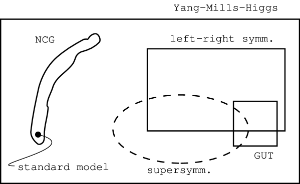
Figure 1: Pseudo forces from noncommutative geometry

The first class is tiny, but still infinite and difficult to assess. We have started putting some order into this class. The criteria we apply are heteroclitic [2].

Two criteria are simply motivated by simplicity: we take the internal algebra to be simple, or with two, three,… simple summands, we take the internal triple to be irreducible.

Two criteria are motivated from perturbative quantum field theory of the non-gravitational part in flat timespace: vanishing Yang-Mills anomalies and dynamical non-degeneracy. The later imposes that the number of possible fermion mass equalities be restricted to the minimum and that they be stable under renormalization flow. The origin of these mass equalities is the following. In almost commutative geometry, the fermionic mass matrix is the ‘Riemannian metric’ of internal space and as such becomes a dynamical variable. Its ‘Einstein equation’ is the requirement that the fermionic mass matrix minimize the Higgs potential. Indeed, in almost commutative geometry, the Higgs potential is the ‘Einstein-Hilbert action’ of internal space.

Two criteria are motivated from particle phenomenology: We want the fermion representation to be complex under the little group in each of its irreducible components, because we want to distinguish particles from anti-particles by means of unbroken charges. We want possible massless fermions to remain neutral under the little group, i.e. not to couple to massless gauge bosons.

Two criteria are motivated from the hope that, one day, we will have a unified quantum theory of all forces: vanishing mixed gravitational Yang-Mills anomalies and again dynamical non-degeneracy.

Our analysis is based on a classification of all finite spectral triples by means of Krajewski diagrams [3] and centrally extended spin lifts of the automorphism group of their algebras [4]. The central extension serves two purposes: (i) It makes the spin lift of complex algebras $M_{n}(\mathbb{C})$ well defined. (ii) It allows the corresponding $U(n)$ anomalies to cancel.

Of course we started with the case of a simple internal algebra. Here there is only one contracted, irreducible Krajewski diagram and all induced Yang-Mills-Higgs models are dynamically degenerate.

The second case concerns algebras with two simple summands. It admits three contracted, irreducible Krajewski diagrams, one of them being a direct sum of two diagrams from the first case. The corresponding triples induce two Yang-Mills-Higgs models which are dynamically non-degenerate and anomaly free: $SU(2)$ with a doublet of left-handed fermions and a singlet of right-handed fermions. The Higgs scalar is a doublet. Therefore the little group is trivial, $SU(2)\rightarrow\{1_{2}\}$, and the fermion representation is real under the little group. The second model is the $SO(2)$ submodel of the first.

The case of three summands has 41 contracted, irreducible diagrams plus direct sums. Its combinatorics is on the limit of what we can handle without a computer. There are only four induced models satisfying all criteria: The first is the standard model with $C$ colours, $C\geq 2$, $SU(2)\times U(1)\times SU(C)$, with one generations of leptons and quarks and one colourless $SU(2)$ doublet of scalars. The three others are submodels, $SO(2)\times U(1)\times SU(C)$, $SU(2)\times U(1)\times SO(C)$ and $SU(2)\times U(1)\times USp(C/2)$ and must have $C\geq 2$, the last submodel of course requires $C$ even, $C\geq 4$.

In the following we push our classification to four summands. For simplicity we will only consider diagrams made of letter changing arrows, i.e. we exclude arrows of type $a\ \bar{a}$ because in the first three cases these arrows always produced degeneracy. When the algebra is simple, of course all arrows are of this type and all models were degenerate. All direct sum diagrams in cases two and three necessarily contain such arrows. For two summands, there is only one contracted, irreducible diagram, that is not a direct sum and that is made of letter changing arrows, for three summands there are 30 such diagrams.

For four summands, a well educated computer [5] tells us that there are 22 contracted, irreducible diagrams made of letter changing arrows and which are not direct sums. They are shown in fig.2. We have two pleasant surprises: (i) the number of these diagrams is small, (ii) there are only two ladder diagrams, diagrams 18 and 19, i.e. diagrams with vertically aligned arrows, and all other diagrams have no subdiagrams of ladder form. We will see that these other diagrams are easily dealt with.

2 Statement of the result

Consider a finite, real, $S^{0}$-real, irreducible spectral triple whose algebra has four simple summands and the extended lift as described in [4]. Consider the list of all Yang-Mills-Higgs models induced by these triples and lifts. Discard all models that have either

• a dynamically degenerate fermionic mass spectrum,

• Yang-Mills or gravitational anomalies,

• a fermion multiplet whose representation under the little group is real or pseudo-real,

• or a massless fermion transforming non-trivially under the little group.

The remaining models are the following, $C$ is the number of colours, the gauge group is on the left-hand side of the arrow, the little group on the right-hand side:

$C=3,5...$

$$\frac{SU(2)\times U(1)\times SU(C)}{\mathbb{Z}_{2}\times\mathbb{Z}_{C}} \longrightarrow \frac{U(1)\times SU(C)}{\mathbb{Z}_{C}}$$

The left-handed fermions transform according to a multiplet ${\underline{2}}\otimes{\underline{C}}$ with hypercharge $q/(2C)$ and a multiplet ${\underline{C}}$ with hypercharge $-q/2$. The right-handed fermions sit in two multiplets ${\underline{C}}$ with hypercharges $q(1+C)/(2C)$ and $q(1-C)/(2C)$ and one singlet with hypercharge $-q$, $q\in\mathbb{Q}$. The elements in $\mathbb{Z}_{2}\times\mathbb{Z}_{C}$ are embedded in the center of $SU(2)\times U(1)\times SU(C)$ as

$$\left(\exp{\frac{2\pi ik}{2}}\,1_{2}\,,\,\exp[2\pi i(Ck-2\ell)/q]\,,\,\exp{\frac{2\pi i\ell}{C}}\,1_{p}\right),\quad k=0,1,\quad\ell=0,1,...,C-1.$$

The Higgs scalar transforms as an $SU(2)$ doublet, $SU(C)$ singlet and has hypercharge $-q/2$.

With the number of colours $C=3$, this is the standard model with one generation of quarks and leptons.

We also have in our list two submodels of the above model defined by the subgroups

$$\frac{SO(2)\times U(1)\times SU(C)}{\mathbb{Z}_{2}\times\mathbb{Z}_{C}} \longrightarrow \frac{U(1)\times SU(C)}{\mathbb{Z}_{C}},$$ (1)

$$\frac{SU(2)\times U(1)\times SO(C)}{\mathbb{Z}_{2}} \longrightarrow U(1)\times SO(C).$$

They have the same particle content as the standard model, in the first case only the $W^{\pm}$ bosons are missing, in the second case roughly half the gluons are lost.

$C=2,4...$

$$\frac{SU(2)\times U(1)\times SU(C)}{\mathbb{Z}_{C}} \longrightarrow \frac{U(1)\times SU(C)}{\mathbb{Z}_{C}}$$

with the same particle content as for odd $C$. But now we have three possible submodels:

$$\frac{SO(2)\times U(1)\times SU(C)}{\mathbb{Z}_{C}} \longrightarrow \frac{U(1)\times SU(C)}{\mathbb{Z}_{C}}\,,$$ (4)

$${SU(2)\times U(1)\times SO(C)} \longrightarrow {U(1)\times SO(C)},$$ (7)

$$\frac{SU(2)\times U(1)\times USp(C/2)}{\mathbb{Z}_{2}} \longrightarrow \frac{U(1)\times USp(C/2)}{\mathbb{Z}_{2}}.$$

electro-strong

$${U(1)\times SU(C)} \longrightarrow {U(1)\times SU(C)}$$

The fermionic content is ${\underline{C}}\oplus{\underline{1}}$, one quark and one charged lepton. The two fermion masses are arbitrary but different and nonvanishing. The number of colours is greater than or equal to two, the two charges are arbitrary but vectorlike, of course the lepton charge must not vanish. There is no scalar and no symmetry breaking.

3 Diagram by diagram

We will use the following letters to denote algebra elements and unitaries: Let $\mathcal{A}=M_{A}(\mathbb{C})\oplus M_{B}(\mathbb{C})\oplus M_{C}(\mathbb{C})\oplus M_{D}(\mathbb{C})\owns(a,b,c,d)$. The extended lift is defined by

$$L(u,v,w,z):=\rho(\hat{u},\hat{v},\hat{w},\hat{z})\,J\rho(\hat{u},\hat{v},\hat{w},\hat{z})J^{-1}$$ (10)

with

$$\hat{u} := u\,(\det u)^{q_{11}}(\det v)^{q_{12}}(\det w)^{q_{13}}(\det z)^{q_{14}}\in U(A),$$ (11)

$$\hat{v} := v\,(\det u)^{q_{21}}(\det v)^{q_{22}}(\det w)^{q_{23}}(\det z)^{q_{24}}\in U(B),$$ (12)

$$\hat{w} := w\,(\det u)^{q_{31}}(\det v)^{q_{32}}(\det w)^{q_{33}}(\det z)^{q_{34}}\in U(C),$$ (13)

$$\hat{z} := z\,(\det u)^{q_{41}}(\det v)^{q_{42}}(\det w)^{q_{43}}(\det z)^{q_{44}}\in U(D),$$ (14)

and unitaries $(u,v,w,z)\in U(M_{A}(\mathbb{C})\oplus M_{B}(\mathbb{C})\oplus M_{C}(\mathbb{C})\oplus M_{D}(\mathbb{C}))$. It is understood that for instance if $A=1$ we set $u=1$ and $q_{j1}=0$, $j=1,2,3,4$. If $M_{A}(\mathbb{C})$ is replaced by $M_{A}(\mathbb{R})$ or $M_{A/2}(\mathbb{H})$ we set $q_{j1}=0$ and $q_{1j}=0$.

Diagram 1 yields:

$$\rho_{L}=\pmatrix{b\otimes 1_{A}&0\cr 0&d\otimes 1_{C}}, \rho_{R}=\pmatrix{a\otimes 1_{A}&0\cr 0&{}^{\alpha}a\otimes 1_{C}},$$ (15)

$$\rho_{L}^{c}=\pmatrix{1_{B}\otimes\,^{\alpha^{\prime}}a&0\cr 0&1_{D}\otimes c}, \rho_{R}^{c}=\pmatrix{1_{A}\otimes\,^{\alpha^{\prime}}a&0\cr 0&1_{A}\otimes c},$$ (18)

and

$$\mathcal{M}=\pmatrix{M_{1}\otimes 1_{A}&0\cr 0&M_{2}\otimes 1_{C}},\quad M_{1}\in M_{B\times A}(\mathbb{C}),\ M_{2}\in M_{D\times A}(\mathbb{C}).$$ (19)

The parameters $\alpha$ and $\alpha^{\prime}$ take values $\pm 1$ and distinguish between fundamental representation and its complex conjugate: ${}^{1}a:=a$, ${}^{-1}a:=\bar{a}$. The colour algebras consist of $a$s and $c$s. The $a$s are broken and therefore we must have $A=1$. We want at most one massless Weyl fermion, which leaves us with three possibilities. The first is $B=2,\ D=1$. The fluctuations read:

$$\varphi_{1}=\sum_{j}r_{j}\,\hat{v}_{j}M_{1}\hat{u}_{j}^{-1},\quad\varphi_{2}=\sum_{j}r_{j}\,\hat{z}_{j}M_{2}\,^{\alpha}\hat{u}_{j}^{-1}.$$ (20)

We can decouple the two scalars $\varphi_{1}$ and $\varphi_{2}$ by means of the fluctuation: $r_{1}={\textstyle\frac{1}{2}},$ $\hat{u}_{1}=1,$ $\hat{v}_{1}=1_{2},$ $\hat{w}_{1}=1_{C}$, $\hat{z}_{1}=1$, $r_{2}={\textstyle\frac{1}{2}},$ $\hat{u}_{2}=1,$ $\hat{v}_{2}=-1_{2},$ $\hat{w}_{2}=1_{C}$, $\hat{z}_{2}=1$. Since the arrows $M_{1}$ and $M_{2}$ are disconnected, the Higgs potential is a sum of a potential in $\varphi_{1}$ and of a potential in $\varphi_{2}$. The minimum is $\stackrel{{\scriptstyle\circ}}{{\varphi}}_{1}=\mu{(4\lambda})^{-\frac{1}{2}}\pmatrix{1\cr 0}$ and $\stackrel{{\scriptstyle\circ}}{{\varphi}}_{2}=\mu{(4\lambda})^{-\frac{1}{2}}$ and the model is dynamically degenerate. The same accidents happen for the second possibility, $B=1,\ D=2$. We are left with the third possibility, $B=D=1$. Anomaly cancellations imply that the fermion couplings are vectorial: $q_{13}=q_{23}$, $q_{43}=\alpha q_{13}$, and there is no spontaneous symmetry breaking, $SU(C)\times U(1)\,\rightarrow\,SU(C)\times U(1)$. The model describes electro-strong forces with one charged lepton, one quark and no scalar. The masses of both fermions are arbitrary but nonvanishing, the electric charges are arbitrary, nonvanishing for the lepton, and the number of colours $C$ is arbitrary, $C\geq 2$.

Diagrams 3, 4 and 7 are treated in the same way and produce only the electro-strong model.

Diagram 2 yields:

$$\rho_{L}=\pmatrix{b\otimes 1_{A}&0\cr 0&{}^{\alpha}a\otimes 1_{C}}, \rho_{R}=\pmatrix{a\otimes 1_{A}&0\cr 0&d\otimes 1_{C}},$$ (21)

$$\rho_{L}^{c}=\pmatrix{1_{B}\otimes\,^{\alpha^{\prime}}a&0\cr 0&1_{A}\otimes c}, \rho_{R}^{c}=\pmatrix{1_{A}\otimes\,^{\alpha^{\prime}}a&0\cr 0&1_{D}\otimes c},$$ (24)

and

$$\mathcal{M}=\pmatrix{M_{1}\otimes 1_{A}&0\cr 1_{A}\otimes M_{3}&M_{2}\otimes 1_{C}},\quad M_{1}\in M_{B\times A}(\mathbb{C}),\ M_{2}\in M_{A\times D}(\mathbb{C}),\ M_{3}\in M_{C\times A}(\mathbb{C}).$$ (25)

If $M_{3}=0$ diagram 2 is treated as diagram 1. We consider the case $M_{3}\not=0$. Then the first order axiom implies $\alpha=1$. The colour algebras consist of $a$s and $c$s. Both are broken and we take $A=C=1$. Then $\mathcal{M}$ is of rank two or less. If we want at most one massless Weyl fermion, we must take $B=2$ and $D=1$ or $B=1$ and $D=2$. Anomaly cancellations then imply that the doublet of fermions does not couple to the determinant of the $2\times 2$ unitary, ‘the hypercharge of the doublet is zero’. On the other hand the little group turns out either trivial or $U(1)$. In the latter case the neutrino sitting in the doublet is charged under this $U(1)$.

Diagram 5 has no unbroken colour and fails as the first possibility of diagram 1, $B=2,\ D=1$.

Diagram 6 has colour $a$ and $b$, both are broken implying $A=B=1$. Then we must have $C=D=1$ to avoid two or more neutrinos.

Diagram 8 yields

$$\rho_{L}=\pmatrix{a\otimes 1_{C}&0\cr 0&c\otimes 1_{B}}, \rho_{R}=\pmatrix{a\otimes 1_{A}&0\cr 0&d\otimes 1_{C}},$$ (26)

$$\rho_{L}^{c}=\pmatrix{1_{A}\otimes\,^{\gamma}c&0\cr 0&1_{C}\otimes b}, \rho_{R}^{c}=\pmatrix{1_{A}\otimes b&0\cr 0&1_{D}\otimes b},$$ (29)

and

$$\mathcal{M}=\pmatrix{1_{A}\otimes M_{1}&0\cr M_{3}\otimes 1_{B}&M_{2}\otimes 1_{B}},\quad M_{1}\in M_{C\times B}(\mathbb{C}),\ M_{2}\in M_{C\times D}(\mathbb{C}),\ M_{3}\in M_{C\times A}(\mathbb{C}).$$ (30)

We suppose that $M_{3}$ does not vanish otherwise diagram 8 is treated as diagram 1. Broken colour implies $A=B=1$. Neutrino counting leaves two possibilities, $C=1$ and $D=2$ or $C=D=2$. The first possibility is disposed of as in diagram 2. For the second possibility, anomaly cancellations imply that the determinants of the $2\times 2$ unitaries $w$ and $z$ do not couple to the right-handed fermions.

Diagrams 14, 15, 16 and 17 share the fate of diagram 6.

Diagram 9 yields

$$\rho_{L}=\pmatrix{b\otimes 1_{A}&0&0\cr 0&c\otimes 1_{B}&0\cr 0&0&d\otimes 1_{D}}, \rho_{R}=\pmatrix{a\otimes 1_{A}&0&0\cr 0&{}^{\beta_{1}}b\otimes 1_{B}&0\cr 0&0&{}^{\beta_{2}}b\otimes 1_{D}},$$ (31)

$$\rho_{L}^{c}=\pmatrix{1_{B}\otimes\,^{\alpha^{\prime}}a&0&0\cr 0&1_{C}\otimes\,^{\beta^{\prime}}b&0\cr 0&0&1_{D}\otimes\,^{\delta^{\prime}}d}, \rho_{R}^{c}=\pmatrix{1_{A}\otimes\,^{\alpha^{\prime}}a&0&0\cr 0&1_{B}\otimes\,^{\beta^{\prime}}b&0\cr 0&0&1_{B}\otimes\,^{\delta^{\prime}}d},$$

and

$$\mathcal{M}=\pmatrix{M_{1}\otimes 1_{A}&1_{B}\otimes M_{4}&1_{B}\otimes M_{5}\cr 0&M_{2}\otimes 1_{B}&0\cr 0&0&M_{3}\otimes 1_{D}}$$ (34)

with $M_{1}\in M_{B\times A}(\mathbb{C}),\ M_{2}\in M_{C\times D}(\mathbb{C}),\ M_{3}\in M_{D\times B}(\mathbb{C}),\ M_{4}\in M_{A\times B}(\mathbb{C}),\ M_{5}\in M_{A\times D}(\mathbb{C}).$ If $M_{4}$ is nonzero $\beta_{1}$ must be one and if $M_{5}$ is nonzero $\beta_{2}$ must be one. From broken colour and neutrino counting we have $A=B=D=1$ and $C=2$. Vanishing anomalies imply that the first and the third fermion have vectorlike hypercharges, while the hypercharges of the second fermion are zero. It is therefore neutral under the little group $U(1)$.

Diagrams 10, 11, 12 and 13 fail in the same way.

Diagram 18 produces the following triple:

$$\rho_{L}=\pmatrix{a\otimes 1_{C}&0\cr 0&{}^{\alpha}a\otimes 1_{D}}, \rho_{R}=\pmatrix{b\otimes 1_{C}&0&0\cr 0&{}^{\beta_{1}}\bar{b}\otimes 1_{C}&0\cr 0&0&{}^{\beta_{2}}\bar{b}\otimes 1_{D}},$$ (35)

$$\rho_{L}^{c}=\pmatrix{1_{A}\otimes c&0\cr 0&1_{A}\otimes d\cr}, \rho_{R}^{c}=\pmatrix{1_{B}\otimes c&0&0\cr 0&1_{B}\otimes c&0\cr 0&0&1_{B}\otimes d},$$

and

$$\mathcal{M}=\pmatrix{M_{1}\otimes 1_{C}&M_{2}\otimes 1_{C}&0\cr 0&0&M_{3}\otimes 1_{D}},\quad M_{1},\ M_{2},\ M_{3}\in M_{A\times B}(\mathbb{C}).$$ (38)

Counting neutrinos leaves two possibilities, $A=2$ and $B=1$, or $A=1$ and $B=1$. If the neutrino is to be neutral under the little group we must have $D=1$ for the first possibility and $C=1$ for the second.

The first possibility has two $U(1)$s if $C\geq 2$ and all four algebras consist of matrices with complex entries. They are parameterized by $\det u$ and by $\det w$. For $(\alpha,\beta_{1},\beta_{2})=+++,\ -++,\ ++-$, and $-+-$, anomaly cancellations imply that the fermionic hypercharges of both $U(1)$s are proportional:

$$q_{11}=-{\textstyle\frac{1}{2}},\ q_{21}=Cp, q_{31}=p,\quad\quad\ q_{41}=-Cp,$$ (39)

$$q_{13}=0,\quad\ q_{23}=Cq, q_{33}=q-{\textstyle\frac{1}{C}},\ q_{43}=-Cq,$$ (40)

with $p,q\in\mathbb{Q}$. Consequently one linear combination of the two generators decouples from the fermions and is absent from the spectral action. This is similar to what happens to the scalar in the electro-strong model of diagram 1. The hypercharges of the remaining generator are those of the standard model with $C$ colours. In the remaining four cases $(\alpha,\beta_{1},\beta_{2})=+-+,\ --+,\ +--,$ and$---$, all 10 fermionic hypercharges vanish and the three leptons are neutral under the little group. Finally the cases where some of the four summands consist of matrices with real or quaternionic entries are treated as in the situation with three summands and they produce the same submodels of the standard model.

The first possibility with $C=1$ has only one $U(1)$. For the four sign assignments: $(\alpha,\beta_{1},\beta_{2})=+++,\ -++,\ ++-$, and $-+-$, we find anomaly free lifts with non-trivial little group. E.g. for the first assignment, we get $q_{11}=-1/2$, $q_{21}=p$, $q_{31}=-p$, and $q_{41}=-p$, with $p\in\mathbb{Q}$. All four assignments produce the electro-weak model $(SU(2)\times U(1))/\mathbb{Z}_{2}\rightarrow U(1)$ of protons, neutrons, neutrinos and electrons.

The second possibility, $A=B=C=1$, contains at least one chiral lepton with vanishing hypercharge and therefore neutral under the little group.

Diagram 19 gives the same results as diagram 18.

In diagrams 20, 21 and 22, the elements $a$ and $b$ must be matrices with complex entries to allow for conjugate representations. Without both the fundamental representation and its complex conjugate these diagrams would violate the condition that every nonvanishing entry of the multiplicity matrix of a (blown up) Krajewski diagram must have the same sign as its transposed element if the latter is not zero. Diagram 20 is treated and fails as diagram 2, diagrams 21 and 22 are treated and fail as diagram 13.

At this point we have exhausted all diagrams of figure 2.

4 Conclusion and outlook

For three summands there was essentially one irreducible spectral triple satisfying all items on our shopping list: the standard model with one generation of quarks and leptons and an arbitrary number of colours (greater than or equal to two). We say ‘essentially’ because a few submodels of the standard model can be obtained. Going to four summands adds precisely one model, the electro-strong model for one massive quark with an arbitrary number of colours and one massive, charged lepton. Note that this is the first appearance of a spectral triple without any Higgs scalar and without symmetry breaking.

We still have to prove that spectral triples in four summands involving letter preserving arrows like $a\ \bar{a}$ do not produce any model compatible with our shopping list.

We are curious to know what happens in five (and more) summands. Here ladder diagrams do not exist and we may speculate that our present list of models exhausts our shopping list also in any number of summands.

Anyhow two questions remain: Who ordered three colours? Who ordered three generations?

diag. 1	diag. 2	diag. 3
diag. 4	diag. 5	diag. 6
diag. 7	diag. 8	diag. 9
diag. 10	diag. 11	diag. 12

diag. 13	diag. 14	diag. 15
diag. 16	diag. 17	diag. 18
diag. 19	diag. 20	diag. 21
diag. 22

References

• [1] A. Connes, Noncommutative Geometry, Academic Press (1994)
A. Connes, Noncommutative geometry and reality, J. Math. Phys. 36 (1995) 6194
A. Connes, Gravity coupled with matter and the foundation of noncommutative geometry, hep-th/9603053, Comm. Math. Phys. 155 (1996) 109
A. Chamseddine & A. Connes, The spectral action principle, hep-th/9606001, Comm. Math. Phys. 182 (1996) 155
• [2] B. Iochum, T. Schücker & C. Stephan, On a classification of irreducible almost commutative geometries, hep-th/0312276, J. Math. Phys, in press
J.-H. Jureit & C. Stephan, On a classification of irreducible almost commutative geometries, a second helping, hep-th/0501134, J. Math. Phys, in press
T. Schücker, Krajewski diagrams and spin lifts, hep-th/0501181
• [3] M. Paschke & A. Sitarz, Discrete spectral triples and their symmetries, q-alg/9612029, J. Math. Phys. 39 (1998) 6191
T. Krajewski, Classification of finite spectral triples, hep-th/9701081, J. Geom. Phys. 28 (1998) 1
• [4] S. Lazzarini & T. Schücker, A farewell to unimodularity, hep-th/0104038, Phys.Lett. B 510 (2001) 277
• [5] J.-H. Jureit & C. Stephan, Finding the standard model of particle physics, a combinatorial problem, hep-th/0503085
$\textstyle{a}$ $\textstyle{b}$ $\textstyle{c}$ $\textstyle{d}$ $\textstyle{a}$ $\textstyle{b}$ $\textstyle{c}$ $\textstyle{d}$        $\textstyle{a}$ $\textstyle{b}$ $\textstyle{c}$ $\textstyle{d}$ $\textstyle{a}$ $\textstyle{b}$ $\textstyle{c}$ $\textstyle{d}$        $\textstyle{a}$ $\textstyle{b}$ $\textstyle{c}$ $\textstyle{d}$ $\textstyle{a}$ $\textstyle{b}$ $\textstyle{c}$ $\textstyle{d}$