CERN-PH-TH/2004-259; OUTP-0502P
Racetrack inflation and assisted moduli stabilisation

Abstract

We present a model of inflation based on a racetrack model without flux stabilization. The initial conditions are set automatically through topological inflation. This ensures that the dilaton is not swept to weak coupling through either thermal effects or fast roll. Including the effect of non-dilaton fields we find that moduli provide natural candidates for the inflaton. The resulting potential generates slow-roll inflation without the need to fine-tune parameters. The energy scale of inflation must be near the GUT scale and the scalar density perturbation generated has a spectrum consistent with WMAP data.

1 Introduction

The issues of hierarchical supersymmetry breakdown and moduli stabilization have long been the central problems of superstring phenomenology. In the original version of the weakly coupled heterotic string these two phenomena are related to each other — once supersymmetry is broken a potential for the moduli fields is generated and their expectation values, hence the parameters of the low energy effective Lagrangian, are determined. If one is to quantify this, the first question to answer is what is the source of supersymmetry breakdown? The next task is to explain how some of the (local or absolute) vacuua of the moduli have just those values which correspond to the observed Universe. Finally one needs to explain how, given that there are many candidate vacuua, just the right one is selected. This latter problem turns out to be particularly difficult to solve because in string-motivated models there always exists a trivial vacuum corresponding to a noninteracting theory. The problem arises because this trivial vacuum is separated from the relevant non-trivial vacuua by an energy barrier which is many orders of magnitude lower than the Planck scale; this follows because of the large hierarchy between the Planck scale and the supersymmetry breaking scale. The problem is that if the initial values for moduli fields are not fine-tuned, the moduli roll so fast that they readily cross the barrier separating the desired minimum from the trivial vacuum. Thus the problem of moduli stabilization is not simply a question of the existence of suitable minima of the potential, it is rather a question about the cosmological dynamics of the theory. These problems have been discussed many times over the last two decades without a satisfactory resolution, see e.g. ref.[1].

Recently a new twist has been added to the discussion in the context of type IIB string compactifications with fluxes. It has been shown that due to the presence of nonzero fluxes of form-fields, all but one of the moduli, including the dilaton but excluding the overall breathing mode of the compact manifold, can be stabilised [2, 3]. The remaining volume modulus can be stabilised with the help of brane-antibrane forces combined with the gaugino-condensation induced nonperturbative potential.  Moreover, in this context the axionic superpartner of the volume modulus can play the role of the cosmological inflaton. To achieve this the authors of ref.[5] invoked a constant piece in the superpotential and the explicitly supersymmetry-breaking term in the scalar potential associated with brane-antibrane forces. However to achieve a significant amount of inflation it proved necessary to fine-tune parameters at the level of one part in a thousand. It was argued on anthropic grounds that such fine-tuning is acceptable. Here we eschew such arguments and look for inflationary solutions which do not involve any fine-tuning — for other relevant proposals see refs.[6, 7].

In this paper we consider these problems in the more traditional setup of ‘racetrack’ models having two gaugino condensates, generated by two asymptotically free non-Abelian hidden gauge sectors in $N=1$ supergravity [8, 9, 10, 11]. Unlike the fluxed models we do not include a constant piece in the superpotential, or break supersymmetry explicitly. We give special attention to the trapping, through topological inflation, of the dilaton at a finite value away from the zero coupling limit at infinity. We discuss how this can avoid the fast-roll problem, and also the problem associated with thermal corrections to the dilaton potential. Although we concentrate on the implications for the weakly coupled heterotic string without fluxes, our results are also relevant to type IIB string compactifications with fluxes. We stress that all this is possible within the well known field-theoretical framework of gaugino-condensation racetrack models; hence the mechanism should be applicable in a wide range of models obtained from various string compactifications.

In Section 2 we discuss how the racetrack potential, through threshold effects, necessarily involves non-dilaton fields, in particular moduli. We discuss how these effects are included in the superpotential and calculate the resulting scalar potential.

In Section 3 we consider how inflation can occur through the slow-roll relaxation of such fields. We show that while slow-roll in the dilaton direction can occur after inflation, the theory is likely to be driven to the free limit. This problem does not occur for the inflationary periods generated by slow-roll in the moduli direction. In this case there is a pseudo-Goldstone inflaton which naturally solves the ‘$\eta$ problem’. We present a numerical study of slow-roll inflation in which we show that the model readily leads to an adequate period of inflation with density perturbations in agreement with observation and a spectral index between 0.96 and 1 (the allowed $1\sigma$ range from WMAP-3 being $0.932\leq n_{s}\leq 0.970$, if a scale-free power-law spectrum is assumed [12]).

In Section 4 we discuss the initial conditions for inflation. We show how the race-track potential necessarily exhibits topological inflation which automatically sets the appropriate initial conditions leading to the slow-roll inflationary era discussed in Section 3. In particular, provided the reheat temperature after inflation is not too large, topological inflation provides a simple mechanism to evade the thermal overshoot problem [13] and avoid the dilaton overshoot problem [14]. We also discuss how the non-inflaton moduli fields are stabilised in a manner that avoids the difficulties discussed in ref. [4]. Finally in Section 5 we present a summary and our conclusions.

2 The gaugino condensation superpotential

There are notable differences between gaugino condensation [15, 16, 17, 18] and fluxes as sources of the superpotential. Perhaps the most important for the present discussion is the fact that the gaugino condensation scale is sensitive to the beta function which in turn is sensitive to the actual mass spectrum at a given energy scale, so the effective nonperturbative potential responds to expectation values of various fields which control the actual mass terms. Fluxes, on the other hand, are imprinted into geometry of the compact manifold and the parameters of the respective superpotential are fixed below the Planck scale. In this paper we will show that the fact that the gaugino condensates take into account the backreaction of other fields on the dilaton provides a natural origin for an inflaton sector. We begin with a discussion of this important backreaction effect.

2.1 The condensation scale

The relation between the field theoretical coupling and the string coupling at the Planck scale is given by

$$\frac{4\pi}{g_{i}^{2}(M)}=\frac{4\pi}{g_{\mathrm{s}}^{2}}+\frac{\Delta_{i}}{4\pi}\ ,$$ (1)

where $\Delta_{i}$ denote string threshold corrections computed at the string scale. The string coupling is related to the dilaton field by $\mathrm{Re}(S)=2\pi/\alpha_{\mathrm{s}}$. At 1-loop the running coupling is given by

$$\frac{1}{\alpha(Q)}=\frac{1}{\alpha(\mu)}+\frac{b_{0}^{\prime}}{2\pi}\log\left(\frac{Q}{\mu}\right),$$ (2)

where for supersymmetric $SU(N)$ with $K$ copies of the vectorlike representation $N+\bar{N}$, the beta function coefficient $b_{0}^{\prime}$ is given by: $b_{0}^{\prime}=3N-K$. The gaugino condensation scale, $\Lambda$, is given approximately by the scale $Q$ at which $1/\alpha(Q)\rightarrow 0$. Using this definition one obtains

$$\Lambda=M\mathrm{e}^{-\mathrm{Re}(S)/b_{0}^{\prime}},$$ (3)

where $M$ is the string cut-off scale, which in leading order corresponds to the gauge coupling unification scale ($5\times 10^{17}$ GeV in the weakly-coupled heterotic string).

The effect of string threshold corrections can be estimated in field theory by including the contribution to the condensation scale from heavy states with mass less than the string cut-off scale, which is typically close to the Planck scale. When the compactification radius is greater than the string radius, the massive fields include those Kaluza-Klein modes lighter than the string scale, but there may be further massive fields which get their mass through a stage of symmetry breaking after compactification.

Now if some gauge non-singlet fields acquire mass $m$ below the string cut-off scale, then the beta function, $b_{0}^{\prime}$, changes to $b_{0}$. In this case the condensation scale acquires an explicit dependence on the scale $m$:

$$\Lambda=M\mathrm{e}^{-\mathrm{Re}(S)/b_{0}}\left|\frac{M}{m}\right|^{(b_{0}^{\prime}-b_{0})/b_{0}}.$$ (4)

We see that the 1-loop threshold correction is of the form $\left|\frac{M}{m}\right|^{(b_{0}^{\prime}-b_{0})/b_{0}}$ which needs to be summed over the contribution of all massive states below the cut-off scale.

2.2 Moduli dependence of the gaugino condensate

In the case the mass, $m$, has a dependence on the vacuum expectation value, $\langle\chi\rangle$, of a scalar field, $\chi$ it is clear that the condensation scale, and hence the dilaton potential which determines the condensation scale, will also depend on $\langle\chi\rangle$. A particularly interesting case is the dependence of the masses on moduli fields. This can arise through the moduli dependence of the couplings involved in the mass generation after a stage of symmetry breakdown. For example a gauge-non singlet field, $\Phi$, may get a mass from a coupling to a field, $\Psi$, when it acquires a vacuum expectation value through a Yukawa coupling in the superpotential of the form $W=\lambda\Psi\Phi\Phi$.  In general the coupling $\lambda$ will depend on the complex structure moduli, $\lambda=\lambda(\langle\chi\rangle)$, and so the mass of the $\Phi$ field will be moduli dependent: $m=\lambda(\langle\chi\rangle)\langle\Psi\rangle$. In what follows we will consider the implications of a very simple dependence of $m$ on the $\langle\chi\rangle$ which is sufficient to illustrate how $\chi$ can provide an inflaton if it is a (modulus) field which has no potential other than that coming from the $m$ dependence of the condensation scale (and the above superpotential coupling). In particular we take $m=\alpha+\beta\langle\chi\rangle$ where $\alpha$ is a mass coming from another sector of the theory, possibly also through a stage of symmetry breaking. With this we have $|m|=|\alpha+\beta\langle\chi\rangle|$ in eq.(4). We shall assume for simplicity a canonical kinetic term for the modulus, $K=\bar{\chi}\chi$, although in practice the form of its Kähler potential may be more complicated.

2.3 The moduli dependent superpotential

Gaugino condensation is described by a nonperturbative superpotential involving the dilaton superfield of the form $W_{\mathrm{npert}}=AN_{1}M^{3}\mathrm{e}^{-S/N_{1}}$ [16, 17, 18]. The question that arises at this point is how to turn the non-holomorphic threshold dependence that enters the condensation scale (4) due to the running in eq.(2) into a holomorphic superpotential. As we have discussed the radiative corrections giving rise to the moduli dependence of the gauge coupling naturally involve the modulus of the mass of the states involved in the loop. However this is because one is calculating the Wilsonian coupling, $g_{\mathrm{c}}$, with canonical kinetic terms, which is not holomorphic. There is a simple relation of this coupling to the holomorphic coupling, $g_{\mathrm{h}}$, with non-canonical kinetic term [19] which is the quantity most closely connected to the superpotential description of gaugino condensation. At the 1-loop level one has

$$\mathrm{Re}\left(\frac{1}{g_{\mathrm{h}}^{2}}\right)=\frac{1}{g_{\mathrm{c}}^{2}}\ .$$ (5)

Since the non-holomorphicity arises from the term proportional to $\log\frac{M}{|\alpha+\beta\langle\chi\rangle|}$ on the rhs of eq.(5), the only way of defining the holomorphic gauge coupling which is consistent with eq.(5) is to replace the absolute value $|\alpha+\beta\langle\chi\rangle|$ appearing under the logarithm by $\alpha+\beta\chi$ itself (i.e. to restore the dependence on the phase of $\chi$). This leads to the holomorphic gauge kinetic function below the scale set by $|\chi|$ of the form

$$f(S,\chi)=\frac{S}{8\pi^{2}}-\frac{b_{0}^{\prime}-b_{0}}{8\pi^{2}}\log\left(\frac{M}{\alpha+\beta\chi}\right),$$ (6)

where the kinetic term of the gauge field has normalisation given by $L_{\mathrm{k}}=\frac{1}{4}\mathrm{Re}(f(S,\chi))F^{2}$. As a consequence, corresponding to the gaugino condensation scale $\Lambda^{3}$ of eq.(3) we have the holomorphic superpotential

$$W=CM^{3}\mathrm{e}^{-24\pi^{2}f(S,\chi)/b_{0}},$$ (7)

where the normalisation factor, $C$, is given in ref.[18].

That this is the correct field dependence of the nonperturbative superpotential can also be seen by considering the supergravity action in its component form with explicit vacuum expectation values for the gaugino bilinears. The relevant part of the scalar potential is

$$V=\mathrm{e}^{K}g^{i\bar{j}}\left(D_{i}W_{\mathrm{pert}}+\frac{1}{4}\mathrm{e}^{-K/2}\partial_{i}f\langle\lambda\lambda\rangle\right)\left(D_{\bar{j}}\bar{W}_{\mathrm{pert}}+\frac{1}{4}\mathrm{e}^{-K/2}\partial_{\bar{j}}\bar{f}\langle\bar{\lambda}\bar{\lambda}\rangle\right).$$ (8)

Following Kaplunovski and Louis [20], we take

$$\langle\lambda\lambda\rangle_{\mathrm{sugra}}=\mathrm{e}^{K/2}\langle\lambda\lambda\rangle_{\mathrm{susy}}=\mathrm{e}^{K/2}M^{3}\mathrm{e}^{-24\pi^{2}f(S,\chi)/b_{0}}.$$

Substituting this into the expression for the scalar potential one finds that contributions coming from condensates are proportional to $\partial_{\chi}W$ and $\partial_{S}W$ with $W$ given by eq.(7) — as is indeed expected.

2.4 The racetrack superpotential

We are now in a position to write down the form of the superpotential corresponding to two gaugino condensates driven by two hidden sectors with gauge group $SU(N_{1})$ and $SU(N_{2})$ respectively. For simplicity we allow for a moduli dependence in the second condensate only. The race-track superpotential has the form

$$W_{\mathrm{npert}}=AN_{1}M^{3}\mathrm{e}^{-S/N_{1}}-BN_{2}M^{3}\mathrm{e}^{-S/N_{2}}\left(\frac{M^{2}}{(\alpha+\beta\chi)^{2}}\right)^{3(N_{2}^{\prime}-N_{2})/(2N_{2})}.$$ (9)

The coefficients $A,\,B$ are related to the remaining string thresholds $\Delta_{i}$ by $A=\mathrm{e}^{-\Delta_{1}/(2N_{1})}/N_{1}$ etc, whose moduli dependence we do not consider here.

3 The racetrack scalar potential

In this paper we will consider a simple model with the dilaton, $S$, the moduli field $\chi$, and the breathing mode of the compact 6-dim space, $T$ which is associated with the overall volume of the compact manifold, $\mathrm{Re}T=V^{1/3}$. We adopt the following standard Kähler potential

$$K(S,\bar{S};T,\bar{T};\chi,\bar{\chi})=-3\log(T+\bar{T})-\log(S+\bar{S})+\chi\bar{\chi}\ ,$$ (10)

where $S=s+i\phi$, $\chi=x\,\mathrm{e}^{i\theta}$, $T=t+i\eta$. An important issue is the freezing of the volume modulus $T$. In particular for the racetrack potential alone there is a runaway direction with $t$ tending to zero. This means $t$ must be fixed by another sector of the theory so we address this issue first.

3.1 Fixing the volume modulus $T$

For the reason just discussed we concentrate here on the $T$ modulus although much of the follwing discussion applies also to other string moduli. The general comment is that, although moduli do not appear on their own in the superpotential and are associated with flat directions, these are lifted after supersymmetry breaking so the moduli will be fixed. In this sense, provided one has a mechanism for supersymmetry breaking, it is not necessary to fix moduli by fluxes. As we now discuss it is not even necessary for supersymmetry breaking to occur for moduli to acquire masses in the absence of fluxes. This can readily happen if there is a stage of spontaneous symmetry breaking in which non-moduli fields acquire vevs which can destroy the flatness of the moduli potential. This is explicitly illustrated below for the $T$ modulus.

In the large volume limit the Kähler potential for the $T$ field assumes the form $K(T,\bar{T})=-3\log(T+\bar{T})$, and that is the form which we have assumed here. The result is that the scalar potential, except the $D$-term contribution, is multiplied by the factor $(2t)^{-3}$. In fact, we do not need to address in detail the issue of low-energy stabilization of $T$ — all we require is that during inflation $t$ should be frozen. There are a number of mechanisms which can do this. The obvious and easiest thing in the present context is if a matter field, $\Phi_{1}$, charged under an anomalous $U(1)$ gauge group has a $T$-dependent kinetic term. This is the case for example for fields carrying non-zero modular weights in heterotic compactifications. Then there appears a $T$-dependent $D$-term contribution to the scalar potential

$$V_{D}=\frac{g^{2}}{2}(f_{1}(t)|\Phi_{1}|^{2}-\xi)^{2},$$ (11)

where $\xi$ arises from the Green-Schwarz term. To preserve supersymmetry, $\Phi_{1}$ must acquire a vev, and this in turn generates a mass for $t$. However it is clear that this term only requires $\langle f_{1}(t)|\Phi_{1}|^{2}\rangle=\xi$, so additional terms must be included to fix the relative value of $\langle\,t\rangle$ and $\langle\Phi_{1}\rangle.$ This can readily happen through the soft mass term $m_{\Phi_{1}}^{2}\left|\Phi_{1}\right|^{2}$. The resulting potential has the form

$$V(T,S,\chi)=V_{\mathrm{RT}}(S,\chi)\frac{(1+\left|\Phi_{1}\right|^{2})}{t^{3}}+\frac{g^{2}}{2}(f_{1}(t)|\Phi_{1}|^{2}-\xi)^{2},$$

where $V_{\mathrm{RT}}(S,\chi)/t^{3}$ is the full racetrack potential and the term $V_{\mathrm{RT}}(S,\chi)\left|\Phi_{1}\right|^{2}/t^{3}$ is the $m_{\Phi_{1}}^{2}\left|\Phi_{1}\right|^{2}$ term during inflation which is automatically present in the supergravity potential. Clearly minimising this with respect to $t$ and $\Phi_{1}$ fixes them independently of the minimisation with respect to $S$ and $\chi$. Note that this means we do not encounter the difficulties found in ref.[4] in their analysis of flux stabilised models where the minimisation must be done simultaneously. For the case $\Phi_{1}$ has a nontrivial modular weight $n_{1}$ we have $f_{1}=(2t)^{-n_{1}}$ and hence $\langle\,t\rangle\simeq\left(\frac{3}{2\xi(n_{1}-3)}\right)^{1/n_{1}}$ for $n_{1}>3$. (For $n_{1}<3$ there is still a minimum at finite $t$ provided the soft mass $m_{\Phi_{1}}^{2}$ is driven negative by radiative corrections at some scale.)

This example illustrates how the $T$ field can be fixed by kinetic terms. Another well known example with $T$-dependent kinetic terms of matter fields are models with a warp factor. In the case of an exponential warp factor the Kähler potential takes the form $K=-3\log(1-\exp(-T-\bar{T}+|\Phi|^{2})-|C|^{2})$ where $\Phi$ denotes warped and $C$ unwarped matter fields. If under a gauge symmetry $T$ transforms nonlinearly, $\delta T=iq\epsilon$, and $\Phi$ and $C$ linearly, $\delta\Phi=i\epsilon Q_{\Phi}\Phi,\,\delta C=i\epsilon Q_{C}C$, then vanishing of the corresponding D-term leads to the approximate relation [21]:

$$\mathrm{e}^{-2t}=\frac{Q_{C}|C|^{2}}{q-Q_{\Phi}|\Phi|^{2}}\ .$$ (12)

So far we have considered the case when there is no $T$ dependence in the superpotential. This has the advantage that the minimum of the potential is at vanishing cosmological constant. When the superpotential depends on $T$, which is often the case, the scalar potential becomes more complicated, and the actual minimum corresponds to negative cosmological constant. This is the situation when one uses target space modular symmetry covariant superpotentials, or when one invokes an exponential superpotential of the form $W_{\mathrm{nonpert}}=AN_{1}\mathrm{e}^{-S/N_{1}}+BN_{2}\mathrm{e}^{-T/N_{2}}-W_{0}$. However, even in such cases it if often possible to argue that the largest term in the potential in the inflationary regime is given by the one we consider, $\mathrm{e}^{K}K^{S\bar{S}}|D_{S}W|^{2}$, with $T$ frozen, for instance by the $D$-term as discussed above.

In fact, the rank of the gauge group permitting, one can stabilise both $S$ and $T$ with the help of condensates and use the inflationary mechanism discussed below to trap both of these moduli. Moreover, if there is a second anomalous $U(1)$ with an assignment of charges such that the Green-Schwarz term $\xi$ cannot be compensated, one has a source of a residual cosmological constant. This may be phenomenologically relevant provided that the moduli dependence leads to a dramatic suppression of its magnitude. Moduli dependent Green-Schwarz terms are associated at the level of the effective 4-dim Lagrangian with gaugings of the imaginary shifts of various moduli fields, $M$. In this case the moduli dependence arises because the Green-Schwarz terms are proportional to $\frac{\partial\,K(M,\bar{M})}{\partial\bar{M}}$ [21]. 

3.2 The racetrack potential

In what follows we assume that one of the mechanisms discussed in the last Section fixes $t$ and allows us to consider the dependence of the racetrack potential only on $S$ and $\chi$. In addition we introduce the notation $\epsilon=(N_{1}-N_{2})/(N_{1}N_{2})$ (assuming $N_{1}>N_{2}$) and $\gamma=3(N_{2}^{\prime}-N_{2})/(2N_{2})$.

For the case of the $T$ independent racetrack superpotential we obtain a positive semi-definite scalar potential for the dilaton and $\chi$-modulus given by

$$V(S)=\frac{1}{2s}\kappa\left|A(2s+N_{1})\mathrm{e}^{-s/N_{1}}-B\mathrm{e}^{-i\epsilon\phi}\left(\alpha+\beta\chi\right)^{-2\gamma}(2s+N_{2})\mathrm{e}^{-s/N_{2}}\right|^{2}\mathrm{e}^{|\chi|^{2}}$$ (13)

$$+\frac{|\chi|^{2}}{2s}\kappa\left|AN_{1}\mathrm{e}^{-s/N_{1}}-B\mathrm{e}^{-i\epsilon\phi}\left(\alpha+\beta\chi\right)^{-2\gamma}N_{2}\mathrm{e}^{-s/N_{2}}\left(1-\frac{2\gamma\beta}{\alpha\bar{\chi}+\beta|\chi|^{2}}\right)\right|^{2}e^{|\chi|^{2}},$$

where $\kappa=1/(8t^{3})$ and the factor $e^{|\chi|^{2}}$ (in Planck units) comes from the factor $\mathrm{e}^{K}$ present in the supergravity potential.

After expanding the perfect squares one obtains a rather complicated function of 4 real variables:

$$V(s,\phi,x,\theta) = \frac{e^{x^{2}}}{2s}\kappa\left(A^{2}(2s+N_{1})^{2}\mathrm{e}^{-2s/N_{1}}+B^{2}(2s+N_{2})^{2}\mathrm{e}^{-2s/N_{2}}[r(x,\theta)]^{-4\gamma}\right.$$ (14)

$$-2AB(2s+N_{1})(2s+N_{2})\mathrm{e}^{-s(\frac{1}{N_{1}}+\frac{1}{N_{2}})}[r(x,\theta)]^{-2\gamma}\cos[\epsilon\phi+2\gamma\delta(x,\theta)]\left.\right)$$

$$+\frac{e^{x^{2}}}{2s}\kappa\left(x^{2}A^{2}N_{1}^{2}\mathrm{e}^{-2s/N_{1}}+B^{2}N_{2}^{2}\mathrm{e}^{-2s/N_{2}}[r(x,\theta)]^{-4\gamma}[r^{\prime}(x,\theta)]^{2}\right.$$

$$-2xABN_{1}N_{2}\mathrm{e}^{-s(\frac{1}{N_{1}}+\frac{1}{N_{2}})}[r(x,\theta)]^{-2\gamma}r^{\prime}(x,\theta)\cos[\epsilon\phi+2\gamma\delta(x,\theta)-\delta^{\prime}(x,\theta)]\left.\right),$$

where

$$r^{2}(x,\theta)=[\alpha+\beta x\cos\theta]^{2}+\beta^{2}x^{2}\sin^{2}\theta,$$

$$r^{\prime}{}^{2}(x,\theta)=\left(x-2\gamma\beta\frac{\beta x+\alpha\cos\theta}{\beta^{2}x^{2}+\alpha^{2}+2\alpha\beta x\cos\theta}\right)^{2}+\frac{4\gamma^{2}\beta^{2}\alpha^{2}\sin^{2}\theta}{(\beta^{2}x^{2}+\alpha^{2}+2\alpha\beta x\cos\theta)^{2}}\ ,$$

$$\tan[\delta(x,\theta)]=\frac{\beta x\sin\theta}{\alpha+\beta x\cos\theta}\ ,$$

$$\tan[\delta^{\prime}(x,\theta)]=\frac{2\gamma\beta\alpha\sin\theta}{\beta^{2}x^{2}+\alpha^{2}+2\alpha\beta x\cos\theta}\left(x-2\gamma\beta\frac{\beta x+\alpha\cos\theta}{\beta^{2}x^{2}+\alpha^{2}+2\alpha\beta x\cos\theta}\right)^{-1}\ .$$ (15)

As discussed above it is consistent to fix $T$ and $\kappa$ independently of the minimisation with respect to $S$ and $\chi$. Thus in the above potential $T$ and $\kappa$ are to be considered constant. Their values provide additional parameters which determine the overall scale of the potential.

3.2.1 Properties of the pure dilaton potential

Given the complexity of the potential it is very difficult to study the most general form as a function of the 4 real variables. As a start to understanding its structure we first study the properties of the purely dilatonic potential.  While we will find that it can generate inflation it suffers from the problem of dilaton overshoot after inflation leading to the non-interacting theory in the post-inflationary era. Thus this Section will serve to motivate the consideration of the more involved potential involving the moduli. The purely dilatonic potential has the form:

$$V(S)=\frac{1}{2s}\left|A(2s+N_{1})\mathrm{e}^{-s/N_{1}}\mathrm{e}^{i\epsilon\phi}-B(2s+N_{2})\mathrm{e}^{-s/N_{2}}\right|^{2}.$$ (16)

This can be written down as a sum of two positive semi-definite terms

$$V(s,\phi)=\frac{1}{2s}\left(A(2s+N_{1})\mathrm{e}^{-s/N_{1}}-B(2s+N_{2})\mathrm{e}^{-s/N_{2}}\right)^{2}$$

$$+\frac{1}{s}AB(2s+N_{1})(2s+N_{2})\mathrm{e}^{-(s/N_{1}+s/N_{2})}\left(1-\cos(\phi\epsilon)\right).$$ (17)

Only the second term depends on the phase $\phi$, and it is minimised for $\phi_{k}=k\,\pi/\epsilon,\;k=0,\pm 1,\pm 2,\ldots$ Notice that the minimum corresponds to a relative minus sign between the two condensates which allows for the cancellation between the terms. This can lead to one or more minima at finite $s$, but, as mentioned above, it may be very difficult to access these minima. For example if initially the phase is displaced from its minimum the cancellation between the terms is no longer complete and the dilaton may be in domain of attraction of the run-away region $s\rightarrow\infty$. We will return in later Sections to the question of how to access minima of the racetrack potential at finite $s$.

It is straightforward to establish that, for $B/A>1$, there is a minimum of the potential at finite $s$ and that the potential vanishes there. We will discuss below whether inflation occurs in the flow from some initial value of $s$ towards this minimum. If $1>B/A>N_{2}/N_{1}$, there is still a minimum at finite $s$ but the potential does not vanish there. Although for the pure dilaton potential this de Sitter minimum is not suitable for generating a finite period of inflation, its existence may be relevant to the case the superpotential has additional moduli dependence allowing for an exit from the de Sitter phase. We will explore this possibility below. Note that in general the first term in the dilaton potential may have up to 4 finite critical points, and one more with infinite vacuum value of the dilaton.

4 Challenges for racetrack inflation

As mentioned in the Introduction, racetrack models have been extensively explored earlier and several difficulties identified which have so far prevented the construction of a viable model (in the absence of fluxes) which can yield inflation and lead to an acceptable Universe afterwards. In this Section we briefly review these difficulties.

4.1 The weak coupling regime of the pure dilaton potential

We first discuss the possibility that, in the pure dilaton potential of eq.(16) there is inflation in the flow to the minimum at finite $s$ in the weak coupling limit. In this limit and assuming the phase of the dilaton field is at its minimum, the position of the minimum and the position of the maximum of the barrier separating it from the minimum at infinity are given by

$$s_{\mathrm{min}}=\frac{1}{\epsilon}\log\left(\frac{B}{A}\right),\quad s_{\mathrm{max}}=\frac{1}{\epsilon}\log\left(\frac{BN_{1}}{AN_{2}}\right).$$ (18)

It is straightforward to check whether the necessary conditions for slow-roll inflation in the $s$ direction are fulfilled at the top of the barrier, i.e. whether $\eta=s^{2}\frac{\partial^{2}V}{\partial s^{2}}\ll 1$. In the large $s$ limit this can be calculated to be

$$\eta=2s_{\mathrm{max}}^{2}\frac{\log(\frac{BN_{1}}{AN_{2}})}{N_{1}-N_{2}},$$ (19)

which is larger than unity in the weak coupling domain, thus slow-roll inflation does not occur.

The other possibility for the pure dilaton potential in the weak coupling domain is slow-roll inflation in the direction of the phase of the dilaton. The slow-roll parameter is now given by: $\eta_{\phi}=(\epsilon s)^{2}\frac{\cos(\epsilon\phi)}{1-\cos(\epsilon\phi)}$.  The requirement that $\eta$ should be much smaller than unity imposes a lower bound on the value of the phase $\phi$. Unfortunately for such high values of the phase, the minimum along the direction of the dilaton has already disappeared — the necessary condition for the presence of that minimum is $\cos^{2}(\epsilon\phi)>4(N_{2}/N_{1})/(1+N_{2}/N_{1})^{2}$, which prefers smaller values of the phase.

4.2 The strong coupling regime and the ‘rapid roll problem’

In order to evade this conclusion and to find a region where inflation can occur it is necessary to move towards the strong coupling domain. In fact there is a saddle-point of the potential (9) in the strong coupling regime which can generate a significant amount of inflation.  However now we face the fundamental problem of explaining how, after inflation, the dilaton moves to the weak coupling minimum at finite $s$ rather than to the non-interacting region $s\rightarrow\infty$. Since the problem occurs at weak coupling it can be reliably estimated even though inflation occurs at strong coupling.

To illustrate the magnitude of the problem we consider a particular example of eq.(16) with $\gamma=3(N_{2}^{\prime}-N_{2})/(2N_{2})=1/2$, $N_{1}=10,\,N_{2}=9,\,A=1$, $B=1.112$. The potential (see Fig. 1) has two minima in the dilaton direction in the strong coupling regime and there is a significant amount of inflation generated in the roll to the minima from the local directional maximum in the direction of $s(z)$.

Figure 1: The shape of the potential in the dilaton $z$ direction (taking $\chi=\alpha=0$) for two illustrative cases: (i) $B=1.112$ — two minima, (ii) $B=1.149$ — a single minimum with vanishing energy (strongly coupled regime).

Of course it is necessary to move from the strong coupling regime at the end of inflation and this can be done by allowing for a moduli dependence of the coefficient $B\rightarrow B\left(1+\beta\chi\right)^{-2\gamma}.$ We should now use the full potential (13) but this still has the relevant saddle-point needed to generate inflation. We now consider the dilaton dependence of the two-condensate potential when the additional field $\chi$ varies. It does so to reduce the vacuum energy and this drives the dilaton to larger values (see Fig. 2), where the form of the potential (13) is reliable.

Figure 2: Sketch of how small change of parameters (represented here by $B$) of the racetrack potential interpolates between the strongly coupled (small $s$) and weakly coupled (large $s$) regimes (arbitrary scales).

In what follows we switch from $s$ to the canonically normalised variable $z=\log(s)$. The problem is that the height of the barrier between the weakly coupled minimum and infinity is very small. We have approximately

$$V_{\mathrm{weak\,barrier}}=m_{3/2}^{2}\left[\frac{8\pi}{g^{2}}+\frac{1}{\epsilon}\log\left(\frac{N_{1}}{N_{2}}\right)\right]\frac{8\pi}{g^{2}},$$ (20)

which for the parameters assumed here is of the order of $10^{-26}$ in Planck units. At the same time it can be seen from Fig. 1 that the vacuum energy during inflation is of order $10^{-2}$ in the same units. Thus the vacuum energy being released is $10^{24}$ times greater than the potential barrier. Even though the fields are damped by expansion during the roll to weak coupling much of this potential energy is converted to kinetic energy and it is overwhelmingly likely that the dilaton will simply jump the barrier between the weakly coupled minimum and infinity and flow to the unphysical decoupling limit. This is the rapid-roll problem emphasised by Brustein and Steinhardt [14].

The underlying problem is that the scale of racetrack potential is dominated by the exponential factors $\mathrm{e}^{-s/N_{1,2}}$, and in the roll from strong to weak coupling these factors require that there is a huge release of potential energy. To avoid this problem it is necessary to look for an inflationary regime which occurs at weak coupling. This offers the possibility of evading the rapid-roll problem because the barrier between the physical minimum and the non-interacting minimum is of order of the vacuum energy during inflation. As discussed above weak coupling inflation does not happen for the pure dilaton potential but we will show that it can occur in the moduli dependent racetrack potential.

4.3 Finite temperature effects and the ‘thermal roll problem’

A related problem to the rapid roll problem is the possibility that thermal effects will drive the dilaton to the non-interacting region $s\rightarrow\infty.$ This has been discussed recently by Buchmüller et al. [13]. The point is that since the couplings of hot matter depend on the dilaton, the free energy of the hot gas adds to the zero-temperature effective potential for the dilaton, and this may change its behaviour if the temperature-dependent piece is sufficiently large. More specifically, the complete dilaton potential is

$$V_{\mathrm{tot}}=V(s)+F(g,T)=V(s)-\frac{\pi^{2}T^{4}}{24}\left(a_{0}+a_{2}g^{2}+\mathcal{O}(g^{3})\right),$$ (21)

where the hot QCD free energy has been taken into account and the gauge coupling $g$ is a function of the dilaton $s$. For the hot QCD plasma, the coefficient $a_{0}$ is positive, but $a_{2}$ is negative so the second term has a minimum for $g=0$. For temperatures above a critical value, $T_{\mathrm{crit}}$, this term fills in the minimum of the $T=0$ dilaton potential at finite $s$ and as a result at high temperatures the dilaton is driven to the non-interacting regime and remains there as the temperature drops. The critical temperature was estimated to be of $\mathcal{O}(10^{13}$) GeV [13]. In the context of inflation driven by the racetrack potential, the problem is that such thermal effects can move the initial conditions far from the saddle point at which inflation occurs.

However there is a straightforward possibility that evades this problem. At a very high value for the Hubble parameter, close to the Planck scale, there is insufficient time for scattering processes to establish thermal equilibrium [22]. In this era the dilaton will not feel the thermal potential and can be in the region where inflation occurs. To quantify this we note that the interaction rate in the quark-gluon gas can be approximated as

$$\Gamma_{\mathrm{int}}=\alpha_{\mathrm{s}}^{2}\,T$$ (22)

and the expansion rate is given by $H_{\mathrm{hot}}=\sqrt{N_{\mathrm{eff}}}T^{2}/M_{\mathrm{P}}$, where $N_{\mathrm{eff}}$ is the effective number of massless degrees of freedom and $M_{\mathrm{P}}\simeq 2.4\times 10^{18}$ GeV is the reduced Planck scale. Requiring that $\Gamma_{\mathrm{int}}>H_{\mathrm{hot}}$ gives the condition for thermal equilibrium:

$$T<T_{\mathrm{eq}}=M_{\mathrm{P}}\frac{\alpha_{\mathrm{s}}^{2}}{\sqrt{N_{\mathrm{eff}}}}.$$ (23)

This means the universe cannot thermalise above $T_{\mathrm{eq}}\sim 10^{15}$ GeV. Although a rough estimate, this is close to the value of $T_{\mathrm{eq}}=3\times 10^{14}$ GeV from a careful analysis [23]. So provided the inflationary potential scale is above $\sqrt{\alpha_{\mathrm{s}}^{2}T_{\mathrm{eq}}M_{\mathrm{P}}}\sim 3\times 10^{15}$ GeV, the thermal-roll problem is avoided.  Of course a viable theory must ensure that the thermal-roll problem does not reappear after inflation in the reheat phase. This simply puts an upper bound on the reheat temperature, $T_{\mathrm{rh}},$ given by $T_{\mathrm{rh}}<T_{\mathrm{eq}}$. This is however far less stringent than the upper bound of $T_{\mathrm{rh}}<10^{8}-10^{10}$ GeV set already by consideration of gravitino production [25], so this will not be a problem in any phenomenologically acceptable model.

5 Inflation from the racetrack potential

We will now argue that the racetrack potential has all the ingredients to meet the challenges just discussed. There are two main aspects to this. Firstly the domain walls generated by the racetrack potential naturally satisfy the conditions needed for topological inflation. As a result there will be eternal inflation within the wall which sets the required initial conditions for a subsequent period of slow-roll inflation during which the observed density perturbations are generated. The second aspect is the existence of a saddle point(s) close to which the potential is sufficiently flat to allow for slow-roll inflation in the weak coupling domain. As noted above this is not the case for the pure dilaton potential but does occur when one includes a simple moduli dependence.

5.1 Topological inflation

As pointed out by Vilenkin [26] and Linde [27], “topological inflation” can occur within a domain wall separating two distinct vacuua. The condition for this to happen is that the thickness of the wall should be larger than the local horizon at the location of the top of the domain wall (we call this the ‘coherence condition’). In this case the initial conditions for slow-roll inflation are arranged by the dynamics of the domain wall which align the field configuration within the wall to minimise the overall energy. The formation of the domain wall is inevitable if one assumes chaotic initial conditions which populate both distinct vacuua and moreover walls extending over a horizon volume are topologically stable. Although the core of the domain wall is stable due to the wall dynamics and is eternally inflating, the region around it is not. As a result there are continually produced regions of space in which the field value is initially close to that at the centre of the wall but which evolve to one or other of the two minima of the potential. If the shape of the potential near the wall is almost flat these regions will generate a further period of slow-roll inflation, at which time density perturbations will be produced.

In the case of the racetrack potential the coherence condition [26] necessary for topological inflation appears to be rather easily satisfied. This condition states that the physical width of the approximate domain wall interpolating between the minimum at infinity and the minimum corresponding to a finite coupling should be larger than the local horizon computed at the location of the top of the barrier that separates them. The width of the domain wall, $\Delta$, is such that the gradient energy stored in the wall equals its potential energy, $\left(\frac{2\delta}{\Delta}\right)^{2}=V(s_{\mathrm{max}})$, where $\delta=\log(s_{\mathrm{max}}/s_{\mathrm{min}})$.  For the racetrack potential (16), the ratio of the width to the local horizon — the coherence ratio — turns out to be:

$$\Delta/H^{-1}=\sqrt{32\pi/3}\log\left(1+N_{1}N_{2}\log(N_{1}/N_{2})/s_{\mathrm{min}}\right).$$ (24)

The weak coupling region corresponds to $s>2\pi$.  Since $s_{\mathrm{min}}\simeq N_{1}N_{2}$ one sees that the coherence ratio is typically larger than 1 in this region.

In fact one can obtain another form for the coherence ratio that demonstrates this more clearly. Close to the top of the domain wall one can approximate the potential in its neighbourhood by the zeroth and quadratic terms in the Taylor expansion: $V(z)=V_{0}-\frac{\mu^{2}}{2}z^{2}$. Let us define the value of $z$ limiting the domain wall as $V(z_{1/n})=V_{0}/n$. Then noticing that the spatial width of the domain wall is such that the potential energy is comparable to the gradient energy $V_{0}=(2z_{1/n})^{2}/\Delta^{2}$ one finds that the ratio $\Delta/H^{-1}$ is inversely proportional to the square root of the slow-roll parameter $\eta=V^{\prime\prime}/V$:

$$\frac{\Delta^{2}}{H^{-2}}=\frac{32\pi}{3}\frac{2(n-1)}{n}\frac{1}{\eta}.$$ (25)

Thus even for $\eta$ of $\mathcal{O}(1)$ the condition for topological inflation is satisfied and even more comfortably so if $\eta$ is as small as is needed for an acceptable spectral index for density perturbations during the slow-roll inflationary period discussed below.

The fact that the racetrack potential readily generates topological inflation offers solutions to all the problems discussed above. With chaotic initial conditions for the dilaton at the Planck era the different vacuua will be populated because the height of the domain walls separating the minima is greater than $T_{\mathrm{eq}}$ so thermal effects will not have time to drive the dilaton to large values. This avoids the initial thermal-roll problem. Then there will be regions of space in which the dilaton rolls from the domain wall value into the minimum at finite $s$, moving from larger to smaller values, and thus avoiding the thermal-roll problem. In fact once created the vacuum bag at finite $s$ is stable, because it cannot move back into the core and over to the other vacuum — the border of the inflating wall escapes exponentially fast — so the respective region of space is trapped in the local vacuum. Finally, if after inflation the reheat temperature is lower than the critical temperature $T_{\mathrm{crit}}$ the thermal effects will be too small to fill in the racetrack minimum at finite $s$ and the region of space in this minimum will remain there, thus avoiding a late thermal-roll problem.

Although the existence of topological inflation seems necessary for a viable inflationary model, by itself it is not sufficient to generate acceptable density perturbations. What is needed is a subsequent period of slow-roll inflation with the appropriate characteristics to generate an universe of the right size ($>50-60$ e-folds of inflation) and density perturbations of the magnitude observed. In the next Section we show that the racetrack potential has the correct properties to achieve this if one includes a simple moduli dependence of the form discussed in Section 2.2.

5.2 Inflation in the weak coupling regime

In this Section we present an example of a viable inflationary model in which the inflaton is the pseudo-Goldstone boson associated with the phase $\theta$ of the field $\chi$.

Figure 3: The $s$ dependence of the potential (in units of $10^{-15}M_{\mathrm{P}}^{4}$) in the neighbourhood of the weakly coupled minimum.

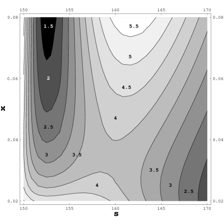
Figure 4: The contour plot in the $s,x$ plane in the neighbourhood of the saddle point. The numbers on the contours give the corresponding values of the scalar potential in units of $10^{-15}M_{\mathrm{P}}^{4}$.

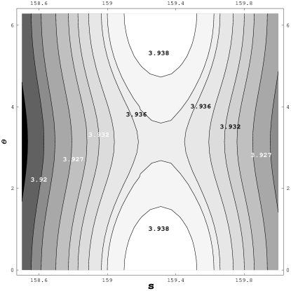
Figure 5: The $\theta$ dependence of the potential in the neighbourhood of the saddle point. Note that the slope along the direction of $\theta$ is much smaller than the slope in the direction of $s$. The numbers on the contours give the corresponding values of the scalar potential in units of $10^{-15}M_{\mathrm{P}}^{4}$.

Figure 6: The “running” of the scalar spectral index, plotted as a function of the number of e-folds from the end of inflation. Note that observationally relevant scales correspond to just the last 5 or so e-folds.

We start with the Kähler potential, eq.(10). The model relies on additional threshold factors of the type discussed in eq.(4) coming from the contribution of additional massive states to the beta function. For simplicity we consider the case that these states have mass given by the vev of $\chi$ up to a coupling constant. The effect of the threshold factors is to add the multiplicative factors $\chi^{p},$ $\chi^{p^{\prime}}$to the two condensates giving the superpotential.

$$W_{\mathrm{npert}}=\chi^{p}AN_{1}M^{3}\mathrm{e}^{-S/N_{1}}-\chi^{p^{\prime}}BN_{2}M^{3}\mathrm{e}^{-S/N_{2}}\left(\frac{M^{2}}{(\alpha+\beta\chi)^{2}}\right)^{3(N_{2}^{\prime}-N_{2})/(2N_{2})}.$$ (26)

Here the exponents $p$ and $p^{\prime}$ are given by the change in the beta functions $(b_{0}^{\prime}-b_{0})/b_{0}$, $c.f.$ $eq.(\ref{fieldthreshold})$. In what follows we consider $p^{\prime}=p$, although typically these powers are different for different gauge sectors. For a range of $p$ and $p^{\prime}$ this simplification does not make a significant difference to the inflationary potential. The analytic expressions for the scalar potentials are not very illuminating, but we give them below for completeness:

$$V(s,\phi,x,\theta) = \frac{\mathrm{e}^{x^{2}}}{2s}\kappa x^{2p}\left(A^{2}(2s+N_{1})^{2}\mathrm{e}^{-2s/N_{1}}+B^{2}(2s+N_{2})^{2}\mathrm{e}^{-2s/N_{2}}[r(x,\theta)]^{-4\gamma}\right.$$ (27)

$$-2AB(2s+N_{1})(2s+N_{2})\mathrm{e}^{-s(\frac{1}{N_{1}}+\frac{1}{N_{2}})}[r(x,\theta)]^{-2\gamma}\cos[\epsilon\phi+2\gamma\delta(x,\theta)]\left.{}\right)$$

$$+\frac{e^{x^{2}}}{2s}\kappa x^{2p}(1+\frac{p}{x^{2}})^{2}\left(x^{2}A^{2}N_{1}^{2}\mathrm{e}^{-2s/N_{1}}+B^{2}N_{2}^{2}\mathrm{e}^{-2s/N_{2}}[r(x,\theta)]^{-4\gamma}r^{\prime}{}^{2}(x,\theta)\right.$$

$$-2xABN_{1}N_{2}\mathrm{e}^{-s(\frac{1}{N_{1}}+\frac{1}{N_{2}})}[r(x,\theta)]^{-2\gamma}r^{\prime}(x,\theta)\cos(\epsilon\phi+2\gamma\delta(x,\theta)-\delta^{\prime}(x,\theta))\left.\right),$$

where

$$r^{2}(x,\theta)=[\alpha+\beta x\cos\theta]^{2}+\beta^{2}x^{2}\sin^{2}\theta),$$

$$r^{\prime}{}^{2}(x,\theta)=\left(x-2\tilde{\gamma}(x)\beta\frac{\beta x+\alpha\cos\theta}{\beta^{2}x^{2}+\alpha^{2}+2\alpha\beta x\cos\theta}\right)^{2}+\frac{4\tilde{\gamma}^{2}(x)\beta^{2}\alpha^{2}\sin^{2}\theta}{(\beta^{2}x^{2}+\alpha^{2}+2\alpha\beta x\cos\theta)^{2}}\ ,$$

$$\tan[\delta(x,\theta)]=\frac{\beta x\sin\theta}{\alpha+\beta x\cos\theta}\ ,$$

$$\tan[\delta^{\prime}(x,\theta)]=\frac{2\tilde{\gamma}(x)\beta\alpha\sin\theta}{\beta^{2}x^{2}+\alpha^{2}+2\alpha\beta x\cos\theta}\left(x-2\tilde{\gamma}(x)\beta\frac{\beta x+\alpha\cos\theta}{\beta^{2}x^{2}+\alpha^{2}+2\alpha\beta x\cos\theta}\right)^{-1}.$$ (28)

and $\tilde{\gamma}(x)=\gamma(1+\frac{p}{x^{2}})^{-1}$. As discussed above it is consistent to fix $T=t+i\eta$ independently of the minimisation with respect to $S$ and $\chi$. Thus in the above potential $\kappa=\kappa(t)$ is to be considered constant. Its value provides an additional parameter which determines the overall scale of the potential.

Numerical analysis of the complete Lagrangian in the $(S,\,\chi)$ hyperplane shows that typically it admits inflationary solutions. A nice example corresponds to the choice of parameters $A=1.5,\;B=8.2,\;N_{1}=10,\;N_{2}=9,\;p=0.5,\;\alpha=1,\;\beta=2.3$ and $\gamma=10^{-4}$. There is a weakly interacting minimum at $s=152.6,\;\phi=0,\;x=0.42$ and $\theta=3.16$ (we remind the reader that $S=s+i\phi$ and $\chi=xe^{i\theta}$). The structure of the potential in the neighbourhood of $s=152.6$ is shown in Figure 3 from which it may be seen that there is a maximum at $s=162.2$. There is a domain wall between the weakly interacting minimum and the non-interacting minimum at $s=\infty$. As may be seen from Figures 4 and 5 it has a saddle point at $s=162.2,$ $\phi=0,$ $x=0.074,$ $\theta=3.152$. Inflation occurs (eternally) within the domain wall and there is further slow-roll inflation outside the wall as it inflates to a size not supported by the dynamics generating it.

The initial conditions for this slow-roll deserve comment. The $s$ field starts very close to the saddle point at $s=162.2$. The same is true for the fields $\phi$ and $x$ which, at the saddle point, have masses larger than the Hubble expansion parameter at this point. However the field $\theta$ is a pseudo-Goldstone field and acquires a mass-squared proportional to $\gamma$. As may be seen from Figure 5, since $\gamma$ is small, the potential is very flat in the $\theta$ direction and the mass of $\theta$ is much smaller than the Hubble expansion parameter. As a result the vev of $\theta$ during the eternal domain wall inflation undergoes a random walk about the saddle point and so its initial value can be quite far from saddle point.

With these initial conditions it is now straightforward to determine the nature of the inflationary period after the fields emerge from the region of the domain wall. This corresponds to the roll of the fields, $s$, $\phi$ and $x$ from the saddle point to the weakly interacting minimum, but allows for $\theta$ to be far from the saddle point. The $s$, $\phi$ and $x$ fields rapidly roll to their minima. However the gradient in the direction of the $\theta$ field is anomalously small due to the pseudo-Goldstone nature of the field. Quantitatively, in the neighbourhood of the weakly interacting minimum, we find a negative eigenvalue of the squared-mass matrix corresponding to the phase $\theta$, and its absolute value is about $10^{4}$ times smaller than the positive eigenvalues. This is much smaller than the Hubble expansion parameter at the start of the roll and so the $\theta$ field indeed generates slow-roll inflation. The remaining degrees of freedom can be integrated out along the inflationary trajectory. Inflation stops after about $7800$ e-folds at $\theta_{\mathrm{e}}=3.54$ and the pivot point corresponds to $\theta_{\star}=4.71$. The value of the curvature of the potential at this point is $\eta_{\star}=-0.0089$ so the scalar spectral index is $n_{\star}\simeq 1+2\eta_{\star}\simeq 0.98$, consistent with the WMAP-3 value at $2\sigma$. The agreement with the normalisation of the spectrum is also readily achieved (we remind the reader that the expectation value of $t$ can be considered as a free parameter for the purpose of tuning the overall height of the inflationary potential, as it is fixed in a separate sector of the model). The evolution of the spectral index during inflation is shown in Figure 6. Note that the ‘running’ of the spectral index is very small, $\mathrm{d}\ln n_{\mathrm{s}}/\mathrm{d}\ln k<\times 10^{-5}$, hence probably undetectable.

To summarise, the moduli dependent racetrack potential has a saddle point which lead to a phenomenologically acceptable period of slow-roll inflation with the inflaton being a component of the moduli. No fine-tuning of parameters is required and the initial conditions are set naturally by the first stage of topological inflation. After inflation there will be a period of reheat and the nature of this depends on the non-inflaton sector of the theory which we have not specified here. From the point of view of the racetrack potential the main constraint on this sector is that the reheat temperature should be less than $T_{\mathrm{crit}}$ to avoid the thermal roll problem. However $T_{\mathrm{crit}}$ is quite high, much higher for example than the maximum reheat temperature allowed by considerations of gravitino production, so this constraint should be comfortably satisfied in any acceptable reheating model.

6 Summary and outlook

There are notable differences between gaugino condensation and fluxes as sources of the superpotential. First of all, the condensation scale is sensitive to the actual mass spectrum at a given energy scale, so the effective nonperturbative potential responds to expectation values of various fields which control the actual mass terms. This readily provides promising candidates for the inflaton field. Fluxes, on the other hand, are imprinted into the geometry of the compact manifold and the parameters of the respective superpotential are fixed below the Planck scale. In fact, the coefficients of these effective superpotentials are quantised in units of the Planck scale, which implies that any lower energy scale can arise only through a miscancellation of these Planck scale terms. By contrast gaugino condensation explains the presence of the inflationary energy scale through logarithmic renormalisation group evolution, and the tuning of the parameters of the effective superpotential can be understood naturally in terms of stringy and field-theoretical threshold corrections.

The formalism developed here takes into account the backreaction of other fields, which must be excited in the early universe, on the dilaton. The resulting inflationary scheme has several attractive features :

• There is an initial period of topological inflation which naturally sets the initial conditions for slow-roll inflation and avoids the rapid-roll and thermal-roll problems usually associated with the racetrack potential. As a result there is no difficulty in having our universe settle in the weakly coupled minimum of the dilaton potential instead of evolving to the runaway non-interacting minimum. This reinstates gaugino condensation as an attractive candidate for supersymmetry breaking.

• The racetrack potential with simple moduli dependence has saddle points which lead to slow-roll inflation capable of generating the observed density fluctuations with a spectral index close to unity. Due to the initial period of topological inflation, the initial conditions for the slow-roll inflation are set automatically without fine-tuning. The fact that one is initially close to a saddle point also means that there is no need to fine-tune the curvature of the potential as is usually necessary for supergravity inflation models.

• The inflationary models constructed here lie within the well known field theoretical framework of gaugino-condensation induced racetrack models. Thus the mechanism should be applicable to a wide range of models obtained from various string-theoretical setups, including models with fluxes. In fact, including the possible effects of fluxes, e.g. a constant piece in the superpotential, or those of warping of the internal space such as an exponential superpotential for the volume modulus $T$, is rather straightforward.

Acknowledgements

We would like to thank Andre Lukas for useful discussions. Z.L. thanks Theoretical Physics of Oxford University for hospitality and S.S. acknowledges a PPARC Senior Research Fellowship (PPA/C506205/1). This work was partially supported by the EC research and training networks MRTN-CT-2004-503369 and HPRN-CT-2000-00152, as well as by the Polish State Committee for Scientific Research (grant KBN 1 P03D 014 26) and POLONIUM 2005.

References

- [1] T. Banks, M. Berkooz, S. H. Shenker, G. W. Moore and P. J. Steinhardt, “Modular cosmology,” Phys. Rev. D 52 (1995) 3548 [arXiv:hep-th/9503114].
- [2] S. Kachru, R. Kallosh, A. Linde and S. P. Trivedi, “De Sitter vacua in string theory,” Phys. Rev. D 68 (2003) 046005 [arXiv:hep-th/0301240].
- [3] R. Kallosh and A. Linde, “Landscape, the scale of SUSY breaking, and inflation,” arXiv:hep-th/0411011.
- [4] K. Choi, A. Falkowski, H. P. Nilles, M. Olechowski and S. Pokorski, “Stability of flux compactifications and the pattern of supersymmetry breaking,” JHEP 0411 (2004) 076 [arXiv:hep-th/0411066].
- [5] J. J. Blanco-Pillado, C. P. Burgess, J. M. Cline, C. Escoda, M. Gomez-Reino, R. Kallosh, A. Linde and F. Quevedo, “Racetrack inflation,” JHEP 0411, 063 (2004) [arXiv:hep-th/0406230].
- [6] R. Brustein, S. P. De Alwis and E. G. Novak, “Inflationary cosmology in the central region of string / M-theory moduli space,” Phys. Rev. D 68 (2003) 023517 [arXiv:hep-th/0205042].
- [7] N. Iizuka and S. P. Trivedi, “An inflationary model in string theory,” Phys. Rev. D 70 (2004) 043519 [arXiv:hep-th/0403203].
- [8] L. J. Dixon, “Supersymmetry breaking in string theory,” SLAC-PUB-5229 Invited talk given at 15th APS Div. of Particles and Fields General Mtg., Houston,TX, Jan 3-6, 1990
- [9] N. V. Krasnikov, “On supersymmetry breaking in superstring theories,” Phys. Lett. B 193 (1987) 37.
- [10] J. A. Casas, Z. Lalak, C. Munoz and G. G. Ross, “Hierarchical supersymmetry breaking and dynamical determination of compactification parameters by nonperturbative effects,” Nucl. Phys. B 347 (1990) 243.
- [11] B. de Carlos, J. A. Casas and C. Munoz, “Supersymmetry breaking and determination of the unification gauge coupling constant in string theories,” Nucl. Phys. B 399 (1993) 623 [arXiv:hep-th/9204012].
- [12] D. N. Spergel et al., “Wilkinson Microwave Anisotropy Probe (WMAP) three year results: Implications for cosmology,” arXiv:astro-ph/0603449.
- [13] W. Buchmuller, K. Hamaguchi, O. Lebedev and M. Ratz, “Dilaton destabilization at high temperature,” Nucl. Phys. B 699 (2004) 292 [arXiv:hep-th/0404168].
- [14] R. Brustein and P. J. Steinhardt, “Challenges for superstring cosmology,” Phys. Lett. B 302, 196 (1993) [arXiv:hep-th/9212049].
- [15] T. R. Taylor, G. Veneziano and S. Yankielowicz, “Supersymmetric QCD and its massless limit: an effective Lagrangian analysis,” Nucl. Phys. B 218, 493 (1983).
- [16] M. Dine, R. Rohm, N. Seiberg and E. Witten, “Gluino condensation in superstring models,” Phys. Lett. B 156 (1985) 55.
- [17] J. P. Derendinger, L. E. Ibanez and H. P. Nilles, “On the low-energy D = 4, N=1 supergravity theory extracted from the D = 10, N=1 superstring,” Phys. Lett. B 155 (1985) 65.
- [18] D. Amati, K. Konishi, Y. Meurice, G. C. Rossi and G. Veneziano, “Nonperturbative aspects in supersymmetric gauge theories,” Phys. Rept. 162, 169 (1988).
- [19] N. Arkani-Hamed and H. Murayama, “Holomorphy, rescaling anomalies and exact beta functions in supersymmetric gauge theories,” JHEP 0006 (2000) 030 [arXiv:hep-th/9707133].
- [20] V. Kaplunovsky and J. Louis, “Field dependent gauge couplings in locally supersymmetric effective quantum field theories,” Nucl. Phys. B 422, 57 (1994) [arXiv:hep-th/9402005].
- [21] R. Ciesielski and Z. Lalak, “Racetrack models in theories from extra dimensions,” JHEP 0212 (2002) 028 [arXiv:hep-ph/0206134].
- [22] J. R. Ellis and G. Steigman, “Nonequilibrium in the very early universe,” Phys. Lett. B 89, 186 (1980).
- [23] K. Enqvist and J. Sirkka, “Chemical equilibrium in QCD gas in the early universe,” Phys. Lett. B 314 (1993) 298 [arXiv:hep-ph/9304273].
- [24] W. H. Kinney, E. W. Kolb, A. Melchiorri and A. Riotto, “Inflation model constraints from the Wilkinson microwave anisotropy probe three-year data,” arXiv:astro-ph/0605338.
- [25] J. R. Ellis, D. V. Nanopoulos and S. Sarkar, “The cosmology Of decaying gravitinos,” Nucl. Phys. B 259 (1985) 175.
- [26] A. Vilenkin, “Topological inflation,” Phys. Rev. Lett. 72, 3137 (1994) [arXiv:hep-th/9402085].
- [27] A. D. Linde and D. A. Linde, “Topological defects as seeds for eternal inflation,” Phys. Rev. D 50, 2456 (1994) [arXiv:hep-th/9402115].