On the invariance under area preserving diffeomorphisms of noncommutative Yang-Mills theory in two dimensions

Abstract:

We present an investigation on the invariance properties of noncommutative Yang-Mills theory in two dimensions under area preserving diffeomorphisms. Stimulated by recent remarks by Ambjorn, Dubin and Makeenko who found a breaking of such an invariance, we confirm both on a fairly general ground and by means of perturbative analytical and numerical calculations that indeed invariance under area preserving diffeomorphisms is lost. However a remnant survives, namely invariance under linear unimodular tranformations.

1 Introduction

Ordinary Yang-Mills theory on a two-dimensional manifold (YM₂) has been long known to be invariant under area preserving diffeomorphisms [1]. Such a symmetry of the classical action is apparent when one realizes that, in two dimensions, the action depends only on the choice of the measure since the field strength of the Yang-Mills field is a two-form. Invariance then follows under all diffeomorphisms which preserve the volume element of the manifold. The theory acquires an almost topological flavor [2] and, as a consequence, quantum YM₂ turns out to be exactly solvable. Beautiful pieces of literature have produced exact expressions for the partition function and Wilson loop averages exploiting such an invariance which led to the discovery of powerful group-theoretic methods [3]. In particular, the derivation of a regular version of the Makeenko-Migdal loop equation by Kazakov and Kostov [4] was possible in two dimensions due to the circumstance that the Wilson loop average for a multiply-intersecting contour depends only on the area of the windows it singles out on the manifold. This property can also be explicitly verified via a perturbative computation in the axial gauge with the principal value prescription, or on the lattice as well, and finds its root in the above mentioned symmetry.

A perturbative computation with all-order resummation for the Wilson loop average was performed in [5]. Invariance under area preserving diffeomorphisms allowed to choose a particular contour, namely a circle, which provides a dramatic simplification in calculations when the Wu-Mandelstam-Leibbrandt [6] prescription for the light-cone gauge propagator is adopted. The authors further probed the invariance performing numerical checks on contours with different shapes. Moreover, a clarification of the role of non-perturbative contributions, and a generalization to contours with arbitrary winding numbers were then obtained in [7], where again the forementioned invariance turns out to play a crucial role.

So far the common lore has been that such an invariance persists in Yang-Mills theories defined on a noncommutative two-dimensional space and it should play a fundamental role inside the large noncommutative gauge group underlying the model. The structure of such a group has been indeed widely investigated because of the intriguing merging of internal and space-time transformations. Its topology, from the very beginning, was argued to be related to $U(\infty)$ and investigated, for example, in [8]. The connection between the large-$N$ limit of $U(N)$ algebras and the algebra of area preserving reparametrizations of two-dimensional tori was elucidated in [9].

A detailed study of the algebra of noncommutative gauge transformations is contained in [10], where they are shown to generate symplectic diffeomorphisms (see also [11]).

The complete gauge transformation is then shown to provide a deformation of the symplectomorphism algebra of $R^{d}$. Finally, since symplectomorphisms in turn coincide with area preserving diffeomorphisms in two dimensions, one might be led to expect that in this case noncommutative Yang-Mills could be exactly solved, exploiting the fact that observables depend purely on the area to apply powerful geometric procedures.

Most of the approaches to this problem start by contemplating the theory on a noncommutative torus. An analysis of the gauge algebra on such a manifold in connection with area preserving diffeomorphisms is presented for example in [12]. There one can exploit Morita equivalence in order to relate the model to its dual on a commutative torus, in which case invariance under area preserving diffeomorphisms is granted. A peculiar limit is then needed to obtain the theory on the noncommutative plane, and one would still expect that the same invariance is there (see for instance [13]).

Wilson loop computations directly on the noncommutative plane and in perturbation theory were performed in [14, 15, 16]. All the results obtained there were consistent with the expected invariance, namely the expansion in the coupling constant and in $1/\theta$, $\theta$ being the noncommutativity parameter, at the orders checked, was found to depend solely on the area.

Recently, however, the authors of [17] were able to extend the results of [14, 15] and found different answers for the Wilson loop on a circle and on a rectangle of the same area. Still, invariance under rotations and symplectic dilatations was expected.

This is the main motivation to dwell on this issue and consider the Wilson loop based on a wide class of contours with the same area. In this paper we limit ourselves to non self-intersecting contours and find that, indeed, invariance under area preserving diffeomorphisms is lost even for smooth contours, the breaking being rooted in the non-local nature of the Moyal product.

A remnant of the invariance is nonetheless retained, precisely the invariance under linear unimodular transformations ($SL(2,R)$).

The issue of volume preserving diffeomorphisms is also crucial in the study of dynamics of noncommutative D-branes [18]. Since noncommutative Yang-Mills theory effectively describes the low-energy behaviour of D-branes embedded in a constant antisymmetric background, the present analysis could be relevant also in a more general string-theoretic context.

The outline of the paper is as follows: In Sect. 2 we prove that $SL(2,R)$ is preserved at any generic order in axial-gauge perturbation theory, provided the gauge-fixing vector is also consistently transformed. We show how the procedure works at ${\cal{O}}(g^{4})$, and how it can be easily generalized. In Sect. 3 we show that the $\theta^{-2}$ term at ${\cal{O}}(g^{4})$ is invariant under $SL(2,R)$, without transforming the gauge vector, by explicitly acting on it with the corresponding algebra generators (technical details are deferred to the Appendix). This term is used in Sect. 4 to perform a series of analytic and numerical computations for a wide class of contours, both smooth and non-smooth, which confirm the outlined picture. In Section 5 we explain why the invariance under area preserving diffeomorphisms, which occurs in ordinary YM₂, is broken to linear $SL(2,R)$ transformations in the noncommutative case. Sect. 6 is finally devoted to our conclusions.

2 Linear transformations: combined shape- and gauge-invariance in perturbation theory

We will concentrate on the noncommutative Euclidean $U(1)$ gauge theory defined on the two-dimensional plane. The results can be easily generalized to the $U(N)$ case. The quantum average of a Wilson loop can be defined by means of the Moyal product as [19] 

$${\cal W}[C]=\int{\cal D}(\tilde{n}A)\,e^{-S[\tilde{n}A]}P_{\star}\exp\left(ig\int_{C}(\tilde{n}A)(z(s))\,\,{{(\tilde{n}\dot{z})}\over{\tilde{n}^{2}}}ds\right)\,,$$ (1)

where $C$ is a closed contour parameterized by $z(s)$, with $0\leq s\leq 1$, $z(0)=z(1)$ and $P_{\star}$ denotes noncommutative path ordering along $z(s)$ from left to right with respect to increasing $s$ of $\star$-products of functions, defined as

$$a*b=\left[\exp{[i{{\theta}\over{2}}\epsilon^{\mu\nu}{\partial}^{x_{1}}_{\mu}{\partial}^{x_{2}}_{\nu}]}a(x_{1})b(x_{2})\right]_{|x_{1}=x_{2}}.$$ (2)

The axial gauge fixing is $nA=0$, $n$ being an arbitrary, fixed vector, and the vector $\tilde{n}$ can be chosen to obey $\tilde{n}_{\mu}=\epsilon_{\mu\nu}n_{\nu}$, so that $n^{2}=\tilde{n}^{2}$ and $n\tilde{n}=0$.

The perturbative expansion of ${\cal W}[C]$, expressed by Eq. (1), reads

$${\cal W}[C] = \sum_{k=0}^{\infty}(ig)^{k}\int_{0}^{1}ds_{1}\ldots\int_{s_{k-1}}^{1}ds_{k}\,{{\tilde{n}\dot{z}(s_{1})}\over{\tilde{n}^{2}}}\ldots{{\tilde{n}\dot{z}(s_{k})}\over{\tilde{n}^{2}}}$$ (3)

$$\phantom{\sum_{k=0}^{\infty}(ig)^{k}}\times\langle 0\left|{\cal T}\left[(\tilde{n}A)(z(s_{1}))\star\ldots\star(\tilde{n}A)(z(s_{k}))\right]\right|0\rangle,$$

and is shown to be an (even) power series in $g$, so that we can write

$${\cal W}[C]=\sum_{k=0}^{\infty}g^{2k}{\cal W}_{2k}\,.$$ (4)

The Moyal phase can be handled in an easier way if we perform a Fourier transform, namely if we work in momentum space. We use the axial gauge propagator $D_{\mu\nu}(p)$, which appears always contracted with $\tilde{n}_{\mu}\tilde{n}_{\nu}$, so that the relevant quantity is $\tilde{n}_{\mu}\,D_{\mu\nu}(p)\,\tilde{n}_{\nu}=n^{2}\tilde{n}^{2}/(np)^{2}$. Each order in the expansion Eq. (4) is indeed a sum of terms like the following

$${\cal W}_{2k}^{\alpha\beta}=\int[ds]\,\tilde{n}\dot{z_{1}}\ldots\tilde{n}\dot{z_{2k}}\int{{d^{2}p_{1}\ldots d^{2}p_{k}}\over{(2\pi)^{2k}}}\,{{1}\over{(np_{1})^{2}\ldots(np_{k})^{2}}}$$ (5)

$$\phantom{{\cal W}_{2k}=\int[ds]\,\tilde{n}\dot{z}(s_{1})\ldots\tilde{n}\dot{z}(s_{2k})}\times\exp\{i\sum_{i<j}^{k}M_{ij}\,p_{i}\wedge p_{j}\}\,\exp\{i\sum_{r=1}^{k}p_{r}\cdot(z_{\alpha(r)}-z_{\beta(r)})\}\,,$$

where $z_{i}$ is a shorthand notation for $z(s_{i})$, $[ds]$ means the suitably ordered measure around the contour and we have taken into account that $n^{4}\,\tilde{n}^{-4}=1$. The notation $\{\alpha(r)<\beta(r)\}$ refers to couples which exhaust the $2k$ positive integers and $M_{ij}$ is a suitable constant antisymmetric matrix. All these quantities depend on the topology of the diagram considered and $p\wedge q\equiv\theta p_{\mu}\epsilon_{\mu\nu}q_{\nu}$.

One can now fairly easily show that the expression above is invariant under linear $SL(2,R)$ transformations provided we rotate the gauge vector accordingly, namely we are considering combined gauge and linear unimodular deformation of the contour. In a noncommutative setting these transformations belong to the $U(\infty)$ gauge invariance group. Since we believe there is independence of the choice of the axial gauge-fixing vector, our result is tantamount to prove invariance under linear deformations of the contour.

In the sequel we shall explicitly exhibit the invariance of the fourth order term ${\cal O}(g^{4})$, but the proof can be straightforwardly generalized to any arbitrary order, i.e. to the generic term appearing in Eq. (5). Eq. (5) leads to the following expression for ${\cal W}_{4}^{np}$, the non-planar contribution to the Wilson loop at ${\cal O}(g^{4})$

$${\cal W}_{4}^{np}=\int[ds]\,\tilde{n}\dot{z}_{1}\ldots\tilde{n}\dot{z}_{4}\int{{d^{2}p\,d^{2}q}\over{(2\pi)^{4}}}\,{{\exp i\{p\wedge q+p(z_{1}-z_{3})+q(z_{2}-z_{4})\}}\over{(np)^{2}\,(nq)^{2}}}\,.$$ (6)

We now perform on $z_{\mu}$ the transformation $z_{\mu}=S_{\mu\nu}\,\xi_{\nu}$, with $\det S=1$, corresponding to the linear unimodular deformation of the contour discussed above. We simultaneously introduce the vectors $P_{\mu}$, $Q_{\nu}$ such that $p_{\mu}=(PS^{-1})_{\mu}$, $q_{\nu}=(QS^{-1})_{\nu}$. It is immediate to verify that $p\wedge q=P\wedge Q$, since the following matrix relation holds

$$S^{-1}\epsilon(S^{-1})^{T}=\epsilon\,,$$ (7)

where the matrix $\epsilon$ is defined as $(\epsilon)_{\mu\nu}=\epsilon_{\mu\nu}$. Then Eq. (6) becomes

$${\cal W}_{4}^{np}=\int[ds]\,(\tilde{n}S\dot{\xi})_{1}\ldots(\tilde{n}S\dot{\xi})_{4}\int{{d^{2}P\,d^{2}Q}\over{(2\pi)^{4}}}\,{{\exp i\{P\wedge Q+P(\xi_{1}-\xi_{3})+Q(\xi_{2}-\xi_{4})\}}\over{(PS^{-1}n)^{2}\,(QS^{-1}n)^{2}}}\,.$$ (8)

The next step consists in defining a new gauge fixing vector according to $\nu=S^{-1}n$ and choosing $\tilde{\nu}$ such that $\tilde{\nu}=\tilde{n}S$. Hence we still have $\tilde{\nu}=\epsilon\nu$ and one can easily realize, with the help of Eq. (7), that the conditions $\nu\tilde{\nu}=0$ and $\tilde{\nu}^{2}=\nu^{2}$ are satisfied. Finally, substituting $n$, $\tilde{n}$ with $\nu$, $\tilde{\nu}$, respectively, in Eq. (8), we conclude our proof, namely that the Wilson loop average, at ${\cal O}(g^{4})$, is invariant under linear $SL(2,R)$ transformations provided we rotate the gauge vector accordingly.

3 $SL(2,R)$ invariance of the coefficient of $\theta^{-2}$ at ${\cal O}(g^{4})$

We prove the invariance under linear deformations of the contour without changing the gauge vector for the $\theta^{-2}$ term in the expansion in $1\over\theta$ of the Wilson loop at ${\cal O}(g^{4})$. This quantity will in turn be used to prove the breaking of the local unimodular invariance in the noncommutative context.

The $\theta^{-2}$ term of the Wilson loop, at the perturbative order $g^{4}$, which will be indicated as $W[C]$ throughout this section for the sake of simplicity, will be computed below for a number of various contours, in order to check whether, and to what extent, invariance under area preserving diffeomorphisms holds. Invariance would imply that $W[C]=kA_{C}^{4}$, where $A_{C}$ is the area enclosed by the contour $C$, the constant $k$ being universal, i.e. independent of the shape of $C$. The starting point for our explicit (both analytical and numerical) computations is [14, 17]

$$W[C]={{g^{4}}\over{4!4\pi^{2}\theta^{2}}}\times$$ (9)

$$\times{\mbox{\bf P}}\!\int\!\int\!\int\!\int{{((x_{1}-z_{1})(y_{2}-t_{2})-(y_{1}-t_{1})(x_{2}-z_{2}))^{4}}\over{(x_{2}-y_{2})^{2}(y_{2}-t_{2})^{2}}}dx_{2}dy_{2}dz_{2}dt_{2}\,,$$

where the integration variables are ordered as $x<y<z<t$ with respect to a given parametrization of $C$ and the subscripts $1,2$ refer to the Euclidean components of the coordinates (the axial gauge is $A_{1}=0$).

This expression can be seen to be equivalent to

$$W[C]= {{g^{4}}\over{4!4\pi^{2}\theta^{2}}}\times\left[A_{C}^{4}+\right.$$ (10)

$$+30\,{\mbox{\bf P}}\!\int\!\int\!\int x_{1}y_{1}z_{1}(x_{1}(y_{2}-z_{2})+y_{1}(z_{2}-x_{2})+z_{1}(x_{2}-y_{2}))\,dx_{2}\,dy_{2}\,dz_{2}+$$

$$+{{5}\over{2}}\oint\oint\left({{4}\over{3}}x_{1}^{3}y_{1}+x_{1}^{2}y_{1}^{2}+{{4}\over{3}}x_{1}y_{1}^{3}\right)(x_{2}-y_{2})^{2}\,dx_{2}\,dy_{2}\,\left.\right]\,,$$

which is particularly suitable for performing calculations since denominators no longer appear. Here the triple integral is ordered according to $x<y<z$, while the double integral is not ordered. Another obvious advantage of Eq. (10) is that, being explicitly finite, it can be run as it stands by a computer program, in order to estimate numerically $W[C]$ for curves that are analytically untractable, such as the even order Fermat curves $C_{2n}\equiv\{(x,y):\ x^{2n}+y^{2n}\ =1$ with $n\geq 1\}$.

The result, as we shall discuss in detail, is that invariance is lost, but a weaker remnant still holds, namely invariance under linear area preserving maps (elements of $SL(2,R)$). Invariance of the quantum average of a Wilson loop under translations is automatic in noncommutative theories owing to the trace-integration over space-time (see also [20]). If we define

$$W[C]={{g^{4}A_{C}^{4}}\over{4!4\pi^{2}\theta^{2}}}\,{\cal I}[C]\,,$$ (11)

it is apparent from Eq. (9) and from dimensional analysis that $\cal I[C]$ is dimensionless and characterizes the shape (and, a priori, the orientation) of a given contour.

Before reporting on specific calculations it is worth showing explicitly that Eq. (9) is invariant under linear area preserving maps. This turns out to be more involved than expected.

A convenient choice for the infinitesimal generators of area preserving diffeomorphisms is given by the set of analytical vector fields

$$\{V_{m,n}\equiv nx_{1}^{m}x_{2}^{n-1}\partial_{x_{1}}-mx_{1}^{m-1}x_{2}^{n}\partial_{x_{2}}\,;(m,n)\in\mathbb{N}\times\mathbb{N}-(0,0)\},$$ (12)

which close on the infinite-dimensional Lie algebra

$$\left[V_{m,n},V_{p,q}\right]=(np-mq)V_{m+p-1,n+q-1}\,.$$

When acting on the coordinates, these generators produce the infinitesimal variations

$$\delta_{V_{m,n}}(x_{1},x_{2})=(nx_{1}^{m}x_{2}^{n-1},-mx_{1}^{m-1}x_{2}^{n})\,,$$

which obviously satisfy the (infinitesimal) unimodularity condition $\partial_{i}\delta x_{i}=0$. We notice that the generators with $n+m\leq 2$ span a finite subalgebra and exponentiate to unimodular inhomogeneous linear maps, namely translations and elements of $SL(2,R)$, while higher level generators exponentiate to non-linear area preserving maps.

Eq. (9) is easily seen to be invariant under translations (which are built in) and under $V_{0,2},V_{1,1}$: the numerator is invariant under linear symplectic maps, and, as far as denominator and measure are concerned, $V_{0,2}$ does not affect the component parallel to the axial gauge vector, while $V_{1,1}$ scales it homogeneously. Indeed Eq. (9) is manifestly invariant under the subgroup generated by $V_{0,2},V_{1,1}$, namely under transformations of the type

$$x_{1}^{\prime}=ax_{1}+bx_{2}\,,\qquad x_{2}^{\prime}=a^{-1}x_{2}\,.$$

A proof of invariance under a third, independent generator, the simplest choice being $V_{2,0}$, can be obtained via the equivalent form Eq. (10) and is presented in the Appendix.

4 Explicit computations for various contours

The computation of the Wilson loop is in principle straightforward for polygonal contours, since only polynomial integrations are required; nonetheless, a considerable amount of algebra makes it rather involved.

Here we summarize our results:

• Triangle: ${\cal I}[\mbox{Triangle}]$ was computed for an arbitrary triangle, the result being ${\cal I}[\mbox{Triangle}]={{8}\over{3}}\simeq 2.6667$. This is consistent with $SL(2,R)$ invariance, since any two given triangles of equal area can be mapped into each other via a linear unimodular map.

• Parallelogram: ${\cal I}[\mbox{Parallelogram}]$ was computed for an arbitrary parallelogram with a basis along $x_{1}$, the result being ${\cal I}[\mbox{Parallelogram}]={{91}\over{36}}\simeq 2.5278$. Again, this is consistent with $SL(2,R)$ invariance, by the same token as above.

• Trapezoid: Here we can see analytically an instance of the broken invariance. Trapezoids of equal area cannot in general be mapped into one other by a linear transformation, since the ratio of the two basis $b_{1}/b_{2}$ is a $SL(2,R)$ invariant. One might say that the space of trapezoids of a given area, modulo $SL(2,R)$, has at least (and indeed, exactly) one modulus, which can be conveniently chosen as the ratio $b_{1}/b_{2}$. Actually, the result we obtained for ${\cal I}[\mbox{Trapezoid}]$ reads

  $${\cal I}[\mbox{Trapezoid}]={{4(6b_{1}^{4}+24b_{1}^{3}b_{2}+31b_{1}^{2}b_{2}^{2}+24b_{1}b_{2}^{3}+6b_{2}^{4})}\over{9(b_{1}+b_{2})^{4}}}\,,$$ (13)

  namely a function of $b_{1}/b_{2}$ only, duly invariant under the exchange of $b_{1}$ and $b_{2}$, and correctly reproducing ${\cal I}[\mbox{Parallelogram}]$ when $b_{1}=b_{2}$, and ${\cal I}[\mbox{Triangle}]$ when $b_{1}=0$. It is plotted in Fig. (1).

  

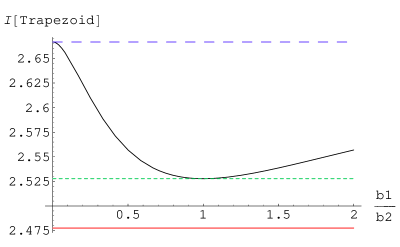
  Figure 1: ${\cal I}[\mbox{Trapezoid}]$ as a function of the ratio of the basis $b_{1}/b_{2}$; the continuous, dashed and dotted straight lines refer to ${\cal I}[\mbox{Circle}]$, ${\cal I}[\mbox{Triangle}]$ and ${\cal I}[\mbox{Square}]$, respectively.

Thus, the main outcome of our computations is that different polygons turn out to produce different results, unless they can be mapped into each other through linear unimodular maps.

As opposed to polygonal contours, smooth contours cannot be in general computed analytically, with the noteworthy exceptions of the circle and the ellipse. A circle can be mapped to any ellipse of equal area by the forementioned area preserving linear maps. Indeed, it is easy to realize from Eq. (10) (because of homogeneity, using the obvious parametrizations), that an ellipse with the axes parallel to $x_{1},x_{2}$ gives the same result as the circle

$${\cal I}[\mbox{Circle}]={\cal I}[{\mbox{Ellipse}}]=1+{{175}\over{12\pi^{2}}}\,$$ (14)

and it turns out to be the lowest value among the (so far computed) non self-intersecting contours. It might be interesting to understand whether this circumstance has any deeper origin. Clearly the same equality does not hold for polygonal contours, e.g. ${\cal I}[{\mbox{Triangle}}]\neq{\cal I}[{\mbox{Circle}}]$.

In the lack of explicit computations for smooth contours, different from circles and ellipses, this scenario might have left open the question whether in the noncommutative case invariance would still be there for smooth contours of equal area, only failing for polygons due to the presence of cusps. We did the check by numeric computations for the (even order) Fermat curves $C_{2n}$ which constitute a family of closed and smooth contours, “interpolating”, in a discrete sense, between two analytically known results, i.e. the circle ($n=1$) and the square (the $n\to\infty$ limit). The numerical computations were performed with two different and independent algorithms, which provided identical results within the level of accuracy required.

As shown in Fig. (2) and in Table (1), ${\cal I}[C_{2n}]$ definitely varies with $n$ and in the $n\to\infty$ limit approaches ${\cal I}[{\mbox{Square}}]$.

Thus we conclude that invariance under area preserving diffeomorphisms does not hold.

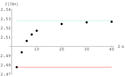
Figure 2: ${\cal I}[C_{2n}]$ for Fermat curves with different $n$; the continuous, dotted lines refer to ${\cal I}[\mbox{Circle}]$, ${\cal I}[\mbox{Square}]$, respectively.

n	1	2	3	4	5	10	15	20
${\cal I}[C_{2n}]$	2.4776	2.4937	2.5060	2.5129	2.5171	2.5243	2.5361	2.5268

Table 1: Numerical results for ${\cal I}[C_{2n}]$ for Fermat curves with different $n$.

Furthermore, we explicitly checked that the numerical results displayed above are invariant (within our numerical accuracy) under rotations of the contours.

By considering higher order generators we were able to show that:

1. All the generators annihilate $W[C]$ on a circle: $\delta_{V_{m,n}}W[C]|_{\mbox{Circle}}=0\,\,\forall(m,n)\,.$ This seems consistent with the fact that $W[\mbox{Circle}]$ is the lowest value among the so far checked non self-intersecting contours, and suggests that actually the circle is likely to be a local weak minimum (of course, there must be flat directions, corresponding to the surviving mentioned symmetries). Nevertheless, the constrained second variation is not easy to compute, and we have not succeeded so far to see whether it is positive semi-definite as we would expect.

2. It was checked by explicit computation that higher level generators do not leave $W[C]$ invariant around a generic triangle. As an example, the variation under $V_{3,0}$ of the triangle defined in the $(x_{1},x_{2})$ plane by the vertices $\{(0,0),(l_{1},h_{1}),(l_{2},h_{2})\}$ is

   $$A_{C}^{4}\cdot\delta_{V_{3,0}}{\cal I}[C]|_{\mbox{Triangle}}={{1}\over{12}}l_{1}l_{2}(l_{1}-l_{2})(l_{1}h_{2}-l_{2}h_{1})^{3}$$

   and vanishes (for non degenerate triangles) only if one of the sides is parallel to the $x_{2}$ axis. Different vanishing conditions arise for different generators, and it can be seen that for no triangle at all is $W[C]$ invariant under the full group of area preserving diffeomorphisms.

5 Arguments concerning invariance under general transformations

Let us provide now a general argument which shows that the expectation value of the Wilson loop is invariant under area preserving diffeomorphisms in ordinary YM₂. We discuss for simplicity the $U(1)$ case.

To start with, let us consider the path integral in $d$ dimensions

$$W[C]=\int{\cal D}Ae^{-S[A]}w[C,A]\,,$$ (15)

where $S[A]={{1}\over{4}}\int F_{ij}F_{kl}\eta^{ik}\eta^{jl}d^{d}x$ is a functional of the vector field $A$, and $w[C,A]=P\exp{i\,\int_{C}A_{i}dx^{i}}$ is a functional of $A$ and of the contour $C$. This has been formulated in cartesian coordinates with metric $\eta_{ij}$. Under a different choice of coordinates $x^{\prime}=x^{\prime}(x)$, $W[C]$ can be rewritten as

$$W[C]=\int{\cal D}Ae^{-S_{gen}[A^{\prime},\,g^{\prime}]}w[C^{\prime},A^{\prime}],$$ (16)

where $S_{gen}[A,g]={{1}\over{4}}\int F_{\mu\nu}F_{\rho\sigma}g^{\mu\nu}g^{\rho\sigma}\sqrt{\det{g}}\,d^{d}x$, provided $A$ and $\eta$ transform to $A^{\prime},g^{\prime}$ like tensors. Notice that $\det{g}$ is positive and the definition of $F_{\mu\nu}$ is left unchanged in the covariantized formulation.

On the other hand, we can consider the same functional computed for the deformed contour $C^{\prime}$

$$W[C^{\prime}]=\int{\cal D}Ae^{-S[A]}w[C^{\prime},A],$$ (17)

the deformation being described by the same map $x^{\prime}=x^{\prime}(x)$ as above.

The condition

$$S_{gen}[A,g^{\prime}]=S[A]$$ (18)

would describe a symmetry of the classical action, which, in dimensions $d>2$, is a tight condition to fulfill. In $d=2$, due to the circumstance that $F_{\mu\nu}$ is a two-form, we get

$$S[A]={{1}\over{2}}\int F_{12}^{2}d^{2}x,$$ (19)

while in $S_{gen}[A,g]$ the contractions with the inverse metric contribute a factor $(\det g)^{-1}$

$$S_{gen}[A,g]={{1}\over{2}}\int F_{12}^{2}{{1}\over{\sqrt{\det{g}}}}d^{2}x.$$ (20)

The condition Eq. (18) then amounts to $\det{g}=1$, which is ensured if the Jacobian of the map is one, namely if $C$ can be deformed to $C^{\prime}$ by an area preserving map.

It is well known that in ordinary YM₂ a Wilson loop depends only on the area it encloses (and not on its shape); thereby the classical symmetry persists at the quantum level, in turn implying ${\cal D}A={\cal D}A^{\prime}$.

When we turn to the noncommutative theory in $d=2$, the expectation value of the Wilson loop becomes

$$W_{nc}[C,*]=\int{\cal D}Ae^{-S_{nc}[A,*]}w_{nc}[C,A,*]\,,$$ (21)

where the Moyal product has been introduced

$$S_{nc}[A,*]={{1}\over{4}}\int F_{ij}*F_{kl}\,\eta^{ik}\eta^{jl}d^{d}x$$

$$w_{nc}[C,A,*]=P_{*}\exp{i\,\int_{C}A_{i}dx^{i}}\,,$$

and the dependence of the involved functionals on $*$ is explicitly exhibited in order to make what follows clear.

Also $W_{nc}$ can be rewritten in general coordinates, provided a covariantized $*^{g}$ product is defined as

$$a*^{g}b=\left[\exp{[i{{\theta}\over{2}}{{\epsilon^{\mu\nu}}\over{\sqrt{\det{g}}}}{\cal D}^{x_{1}}_{\mu}{\cal D}^{x_{2}}_{\nu}]}a(x_{1})b(x_{2})\right]_{|x_{1}=x_{2}},$$ (22)

${\cal D}_{\mu}$ being the covariant derivative associated to the Riemannian connection for the metric $g$.  Under the same reparametrization we then obtain

$$W_{nc}[C,*]=\int{\cal D}Ae^{-S_{nc,gen}[A^{\prime},g^{\prime},*^{g^{\prime}}]}w_{nc}[C^{\prime},A^{\prime},*^{g^{\prime}}],$$ (23)

where the noncommutative action in general coordinates

$$S_{nc,gen}[A,g,*^{g}]={{1}\over{4}}\int F_{\mu\nu}*^{g}F_{\rho\sigma}g^{\mu\nu}g^{\rho\sigma}\sqrt{\det{g}}\,d^{2}x$$ (24)

and Wilson loop

$$w_{nc,gen}[C,A,*^{g}]=P_{*^{g}}\exp{i\,\int A_{\mu}dx^{\mu}}$$ (25)

have been introduced.

Assuming the absence of functional anomalies also in the noncommutative case, we compare Eq. (23) with the functional $W_{nc}[C^{\prime},*]$ computed for the deformed contour $C^{\prime}$

$$W_{nc}[C^{\prime},*]=\int{\cal D}Ae^{-S_{nc}[A,*]}w_{nc}[C^{\prime},A,*].$$ (26)

The two quantities coincide if the following two sufficient conditions are met

• $*^{g}=*$,

• $S_{nc,gen}[A,g^{\prime},*]=S_{nc}[A,*].$

These conditions imply that the map is at most linear, since the Riemannian connection must vanish, and that its Jacobian equals unity. In conclusion, only $SL(2,R)$ linear maps are allowed.

6 Conclusions

Gauge theories defined on a noncommutative two-dimensional manifold were from the beginning believed to be invariant under the group of area preserving diffeomorphisms, as it occurs in their commutative counterparts. This property holding, one would have a deeper understanding of the structure of the noncommutative gauge group underlying these models, and a larger set of geometric tools available for challenging a complete solution. However, a perturbative computation of the Wilson loop revealed a lack of this invariance: at order ${\cal{O}}(g^{4})$ in the coupling constant and ${\cal{O}}(\theta^{-2})$ in the noncommutativity parameter, the Wilson loop $W[C]$ is not the same when evaluated on a circle and on a rectangle of equal area [17]. While this could be the signal of a breaking of invariance under the group of area preserving diffeomorphisms at the perturbative level, the questions of the generalization of this result to other classes of contours, and of the possible existence of unbroken subgroups, immediately arose.

In this paper we reported in detail a number of analytic and numerical computations of the above mentioned term $W[C]$ for a wide choice of different contours. In so doing we confirmed the breaking of the invariance: we found different values for triangles, parallelograms, trapezoids, circles and Fermat curves. An interesting result we found is that the latter nicely interpolate between the values of the the circle and of the square. We pointed out the existence of an unbroken subgroup, namely the one of area preserving linear maps of the plane $SL(2,R)$. We also explained why invariance under a local area preserving diffeomorphism, which is present in the commutative case, cannot persist in the noncommutative context, owing to the non-local nature of the Moyal product, at least perturbatively.

While our findings give a generalized proof of the perturbative breaking of invariance under area preserving diffeomorphisms, some issues deserve further investigation. It would be interesting to possibly extend our results to nonperturbative approaches appeared in the literature [21]. In turn they might also be relevant for the physics of membranes, which is tightly related to noncommutative gauge theories. On another side they may entail important consequences on the analysis of the merging of space-time and internal symmetries in a noncommutative context.

7 Acknowledgements

We thank Jan Ambjorn and Yuri Makeenko for stimulating insights stressing the breaking of the general invariance under area preserving diffeomorphisms in noncommutative YM₂. We are grateful to Pieralberto Marchetti for general comments concerning invariance properties in QFT. Finally, A.T. wishes to thank Harald Dorn, Christoph Sieg and Sebastian de Haro for discussions.

8 Appendix

We show here that Eq. (10) in the main text is invariant under the action of the infinitesimal generator $V_{2,0}$, which can be read from Eq. (12). The proof goes as follows. First we compute the variation of Eq. (10) under a generic infinitesimal tranformation $(\delta x_{1},\delta x_{2})$. Let us indicate the integrands in the triple and double integrals in Eq. (10) as $f(x,y,z)$ and $g(x,y)$ and notice that $f$ is a completely antisymmetric function of its arguments, whereas $g$ is symmetric. Integrating by parts and taking into due account the fact that the curve is closed, which, together with the aforementioned symmetry properties, allows to cancel all the “finite parts”, we find

$$A_{C}^{4}\cdot\delta{\cal I}[C]={{5}\over{2}}\oint\oint[\partial_{x_{1}}g(\delta x_{1}\,dx_{2}dy_{2}-\delta x_{2}\,dx_{1}dy_{2})+\partial_{y_{1}}g(\delta y_{1}\,dx_{2}dy_{2}-\delta y_{2}\,dx_{2}dy_{1})]$$

$$+30\,{\mbox{\bf P}}\!\int\!\!\!\int\!\!\!\int[\partial_{x_{1}}f(\delta x_{1}\,dx_{2}dy_{2}dz_{2}-\delta x_{2}\,dx_{1}dy_{2}dz_{2})+\partial_{y_{1}}f(\delta y_{1}\,dx_{2}dy_{2}dz_{2}-\delta y_{2}\,dx_{2}dy_{1}dz_{2})$$

$$\phantom{30\,{\mbox{\bf P}}\!\int\!\!\!\int\!\!\!\int}+\partial_{z_{1}}f(\delta z_{1}\,dx_{2}dy_{2}dz_{2}-\delta x_{2}\,dx_{2}dy_{2}dz_{1})]\,;$$ (27)

when we specialize the expression above to the $V_{2,0}$ generator, it becomes

$$A_{C}^{4}\cdot\delta_{V_{2,0}}{\cal I}[C]=5\oint\oint[(4x_{1}^{3}y_{1}+2x_{1}^{2}y_{1}^{2}+{{4}\over{3}}x_{1}y_{1}^{3})(x_{2}^{2}-2x_{2}y_{2}+y_{2}^{2})\,dx_{1}dy_{2}$$ (28)

$$\phantom{A_{C}^{4}\cdot\delta_{V_{2,0}}{\cal I}[C]=5\oint[}+({{4}\over{3}}x_{1}^{3}y_{1}+2x_{1}^{2}y_{1}^{2}+4x_{1}y_{1}^{3})(x_{2}^{2}-2x_{2}y_{2}+y_{2}^{2})\,dx_{2}dy_{1}]$$

$$+60\,{\mbox{\bf P}}\!\int\!\!\!\int\!\!\!\int[(2x_{1}^{2}y_{1}z_{1}(y_{2}-z_{2})+x_{1}y_{1}^{2}z_{1}(z_{2}-x_{2})+x_{1}y_{1}z_{1}^{2}(x_{2}-y_{2}))\,dx_{1}dy_{2}dz_{2}$$

$$\phantom{+60\,{\mbox{\bf P}}\!\int\!\!\!\int\!\!\![}+(x_{1}^{2}y_{1}z_{1}(y_{2}-z_{2})+2x_{1}y_{1}^{2}z_{1}(z_{2}-x_{2})+x_{1}y_{1}z_{1}^{2}(x_{2}-y_{2}))\,dx_{2}dy_{1}dz_{2}$$

$$\phantom{+60\,{\mbox{\bf P}}\!\int\!\!\!\int\!\!\![}+(x_{1}^{2}y_{1}z_{1}(y_{2}-z_{2})+x_{1}y_{1}^{2}z_{1}(z_{2}-x_{2})+2x_{1}y_{1}z_{1}^{2}(x_{2}-y_{2}))\,dx_{2}dy_{2}dz_{1}]\,.$$

A few tricks now are useful to simplify Eq. (28), namely:

1. terms in which only one component of one of the points $x,y,z$ appears, such as $x_{1}^{2}dx_{1}$, can be explicitly integrated, giving rise to either ordered double integrals (from the triple integral) or simple loop integrals (from the double one). That is, e.g.

   $$\mbox{\bf P}\!\int\!\int\!\int y_{1}y_{2}z_{1}^{2}x_{1}dx_{1}dy_{2}dz_{2}\to{{1}\over{2}}\mbox{\bf P}\!\int\!\int y_{1}y_{2}(y_{1}^{2}-t_{1}^{2})z_{1}^{2}dy_{2}dz_{2}\,,$$

   $t=(t_{1},t_{2})$ being the starting point of the parametrization;

2. terms in which each point appears with both components, are integrated by parts in the component “1”, e.g. $x_{1}x_{2}dx_{1}=d({{x_{1}^{2}x_{2}}\over{2}})-{{x_{1}^{2}}\over{2}}dx_{2}$, leaving a “lower-order” integral as above, plus an integral where the $dx_{1}$ differential has been traded for $dx_{2}$;

3. an ordered double integral, whose integrand $h$ is symmetric, $h(x,y)=h(y,x)\,,$ amounts to one half of the corresponding unordered integral

   $${\mbox{\bf P}}\!\int\!\int h(x,y)dx_{2}dy_{2}={{1}\over{2}}\oint\oint h(x,y)dx_{2}dy_{2}\,.$$

When all this has been done, we are left with a triple ordered integral with measure $dx_{2}dy_{2}dz_{2}$, whose integrand vanishes. A collection of double, non ordered integrals survives, but it can be shown it cancels as well.

The proof of invariance of $W[C]$ under $SL(2,R)$ is thereby completed.

References

- [1] E. Witten, “On quantum gauge theories in two-dimensions,” Commun. Math. Phys. 141 (1991) 153; “Two-dimensional gauge theories revisited,” J. Geom. Phys. 9 (1992) 303 [arXiv:hep-th/9204083].
- [2] A. A. Migdal, “Recursion Equations In Gauge Field Theories,” Sov. Phys. JETP 42 (1975) 413 [Zh. Eksp. Teor. Fiz. 69 (1975) 810].
- [3] B. E. Rusakov, “Loop Averages And Partition Functions In U(N) Gauge Theory On Two-Dimensional Manifolds,” Mod. Phys. Lett. A 5 (1990) 693; “Large N quantum gauge theories in two-dimensions,” Phys. Lett. B 303 (1993) 95 [arXiv:hep-th/9212090]; M. R. Douglas and V. A. Kazakov, “Large N phase transition in continuum QCD in two-dimensions,” Phys. Lett. B 319 (1993) 219 [arXiv:hep-th/9305047]; D. V. Boulatov, “Wilson loop on a sphere,” Mod. Phys. Lett. A 9 (1994) 365 [arXiv:hep-th/9310041]; J. M. Daul and V. A. Kazakov, “Wilson loop for large N Yang-Mills theory on a two-dimensional sphere,” Phys. Lett. B 335 (1994) 371 [arXiv:hep-th/9310165].
- [4] V. A. Kazakov and I. K. Kostov, “Nonlinear Strings In Two-Dimensional U(Infinity) Gauge Theory,” Nucl. Phys. B 176 (1980) 199; “Computation Of The Wilson Loop Functional In Two-Dimensional U(Infinite) Lattice Gauge Theory,” Phys. Lett. B 105 (1981) 453; V. A. Kazakov, “Wilson Loop Average For An Arbitrary Contour In Two-Dimensional U(N) Gauge Theory,” Nucl. Phys. B 179 (1981) 283.
- [5] M. Staudacher and W. Krauth, “Two-dimensional QCD in the Wu-Mandelstam-Leibbrandt prescription,” Phys. Rev. D 57 (1998) 2456 [arXiv:hep-th/9709101].
- [6] T.T. Wu, “Two-dimensional Yang-Mills theory in the leading expansion,” Phys. Lett. B 71 (1977) 142; S. Mandelstam, “Light-cone superspace and the ultraviolet finiteness of the model,” Nucl. Phys. B 213 (1983) 149; G. Leibbrandt, “The light-cone gauge in Yang-Mills theory.” Phys. Rev. D 29 (1984) 1699; A. Bassetto, M. Dalbosco, I. Lazzizzera and R. Soldati, “Yang-Mills theories in the light-cone gauge,” Phys. Rev. D 31 (1985) 2012.
- [7] A. Bassetto, F. De Biasio and L. Griguolo, “Lightlike Wilson loops and gauge invariance of Yang-Mills theory in (1+1)-dimensions,” Phys. Rev. Lett. 72 (1994) 3141 [arXiv:hep-th/9402029]; A. Bassetto and L. Griguolo, “Two-dimensional QCD, instanton contributions and the perturbative Wu-Mandelstam-Leibbrandt prescription,” Phys. Lett. B 443 (1998) 325 [arXiv:hep-th/9806037]; A. Bassetto, L. Griguolo and F. Vian, “Instanton contributions to Wilson loops with general winding number in two dimensions and the spectral density,” Nucl. Phys. B 559 (1999) 563 [arXiv:hep-th/9906125].
- [8] J. A. Harvey, “Topology of the gauge group in noncommutative gauge theory,” [arXiv:hep-th/0105242].
- [9] D. B. Fairlie, P. Fletcher and C. K. Zachos, “Infinite Dimensional Algebras And A Trigonometric Basis For The Classical Lie Algebras,” J. Math. Phys. 31 (1990) 1088; E. Sezgin, “Area-Preserving Diffeomorphisms, Algebras and Gravity,” [arXiv:hep-th/9202086].
- [10] F. Lizzi, R. J. Szabo and A. Zampini, “Geometry of the gauge algebra in noncommutative Yang-Mills theory,” JHEP 0108 (2001) 032 [arXiv:hep-th/0107115].
- [11] M. R. Douglas and N. A. Nekrasov, “Noncommutative field theory,” Rev. Mod. Phys. 73 (2001) 977 [arXiv:hep-th/0106048].
- [12] M. M. Sheikh-Jabbari, “Renormalizability of the supersymmetric Yang-Mills theories on the noncommutative torus,” JHEP 9906 (1999) 015 [arXiv:hep-th/9903107].
- [13] L. D. Paniak and R. J. Szabo, “Open Wilson lines and group theory of noncommutative Yang-Mills theory in two dimensions,” JHEP 0305 (2003) 029 [arXiv:hep-th/0302162].
- [14] A. Bassetto, G. Nardelli and A. Torrielli, “Perturbative Wilson loop in two-dimensional non-commutative Yang-Mills theory,” Nucl. Phys. B 617 (2001) 308 [arXiv:hep-th/0107147].
- [15] A. Bassetto, G. Nardelli and A. Torrielli, “Scaling properties of the perturbative Wilson loop in two-dimensional non-commutative Yang-Mills theory,” Phys. Rev. D 66 (2002) 085012 [arXiv:hep-th/0205210].
- [16] A. Torrielli, “Noncommutative perturbative quantum field theory: Wilson loop in two-dimensional Yang-Mills, and unitarity from string theory,” PhD thesis [arXiv:hep-th/0301091].
- [17] J. Ambjorn, A. Dubin and Y. Makeenko, “Wilson loops in 2D noncommutative Euclidean gauge theory. I: Perturbative expansion,” JHEP 0407 (2004) 044 [arXiv:hep-th/0406187].
- [18] B. de Wit, J. Hoppe and H. Nicolai, “On The Quantum Mechanics Of Supermembranes,” Nucl. Phys. B 305 (1988) 545; E. Bergshoeff, E. Sezgin, Y. Tanii and P. K. Townsend, “Super P-Branes As Gauge Theories Of Volume Preserving Diffeomorphisms,” Annals Phys. 199 (1990) 340; Y. Matsuo and Y. Shibusa, “Volume preserving diffeomorphism and noncommutative branes,” JHEP 0102 (2001) 006 [arXiv:hep-th/0010040]; E. Langmann and R. J. Szabo, “Teleparallel gravity and dimensional reductions of noncommutative gauge theory,” Phys. Rev. D 64 (2001) 104019 [arXiv:hep-th/0105094].
- [19] N. Ishibashi, S. Iso, H. Kawai and Y. Kitazawa, “Wilson loops in noncommutative Yang-Mills,” Nucl. Phys. B 573 (2000) 573 [arXiv:hep-th/9910004]; D. J. Gross, A. Hashimoto and N. Itzhaki, “Observables of non-commutative gauge theories,” Adv. Theor. Math. Phys. 4 (2000) 893 [arXiv:hep-th/0008075]; L. Alvarez-Gaume and S. R. Wadia, “Gauge theory on a quantum phase space,” Phys. Lett. B 501 (2001) 319 [arXiv:hep-th/0006219].
- [20] M. Abou-Zeid, H. Dorn, “Dynamics of Wilson Observables in Noncommutative Gauge Theory,” Phys. Lett. B 504 (2001) 165 [arXiv:hep-th/0009231].
- [21] L. D. Paniak and R. J. Szabo, “Instanton expansion of noncommutative gauge theory in two dimensions,” Commun. Math. Phys. 243 (2003) 343 [arXiv:hep-th/0203166]; L. Griguolo and D. Seminara, “Classical solutions of the TEK model and noncommutative instantons in two dimensions,” JHEP 0403 (2004) 068 [arXiv:hep-th/0311041]; H. Dorn and A. Torrielli, “Loop equation in two-dimensional noncommutative Yang-Mills theory,” JHEP 0401 (2004) 026 [arXiv:hep-th/0312047]; W. Bietenholz, F. Hofheinz and J. Nishimura, “The renormalizability of 2D Yang-Mills theory on a non-commutative geometry,” JHEP 0209 (2002) 009 [arXiv:hep-th/0203151]; W. Bietenholz, A. Bigarini, F. Hofheinz, J. Nishimura, Y. Susaki and J. Volkholz, “Numerical results for U(1) gauge theory on 2d and 4d non-commutative spaces,” [arXiv:hep-th/0501147].