LPTENS-05/11

LMU-ASC 23/05

hep-th/0503173

Special geometry of local Calabi-Yau manifolds

and superpotentials from holomorphic matrix models
Adel Bilal¹ and Steffen Metzger^1,2

¹ Laboratoire de Physique Théorique, École Normale Supérieure - CNRS

24 rue Lhomond, 75231 Paris Cedex 05, France

² Arnold-Sommerfeld-Center for Theoretical Physics,

Department für Physik, Ludwig-Maximilians-Universität

Theresienstr. 37, 80333 Munich, Germany

e-mail: adel.bilal@lpt.ens.fr, metzger@physique.ens.fr

Abstract

We analyse the (rigid) special geometry of a class of local Calabi-Yau manifolds given by hypersurfaces in $\mathbb{C}^{4}$ as $W^{\prime}(x)^{2}+f_{0}(x)+v^{2}+w^{2}+z^{2}=0$, that arise in the study of the large $N$ duals of four-dimensional $\mathcal{N}=1$ supersymmetric $SU(N)$ Yang-Mills theories with adjoint field $\Phi$ and superpotential $W(\Phi)$. The special geometry relations are deduced from the planar limit of the corresponding holomorphic matrix model. The set of cycles is split into a bulk sector, for which we obtain the standard rigid special geometry relations, and a set of relative cycles, that come from the non-compactness of the manifold, for which we find cut-off dependent corrections to the usual special geometry relations. The (cut-off independent) prepotential is identified with the (analytically continued) free energy of the holomorphic matrix model in the planar limit. On the way, we clarify various subtleties pertaining to the saddle point approximation of the holomorphic matrix model. A formula for the superpotential of IIB string theory with background fluxes on these local Calabi-Yau manifolds is proposed that is based on pairings similar to the ones of relative cohomology.

1 Introduction

Compactifications of string theory on Calabi-Yau manifolds have been studied for almost two decades [1]. One particularly appealing property of Calabi-Yau compactifications is that the special geometry structure of the effective supergravity theory [2] can be understood from the fact that the (Kähler and complex structure) moduli spaces of a Calabi-Yau manifold are special Kähler manifolds. What is more, the prepotential that corresponds to the complex structure deformations can be expressed in terms of period integrals on the Calabi-Yau space [3]. For these periods one can deduce the Picard-Fuchs differential equations and so get interesting physical quantities from the solutions of these equations. In general the computation of the Kähler part is more complicated as in this case the period integrals are corrected by world-sheet instantons. However, mirror symmetry comes to the rescue since the Kähler moduli space of a Calabi-Yau $X$ can be mapped to the complex structure moduli space of its mirror $\tilde{X}$. The Kähler prepotential can then be computed using the mirror map.

To be more precise, if $\mathcal{F}$ is the prepotential on the moduli space of complex structures of a Calabi-Yau manifold $X$, one has the special geometry relations [3]
$\displaystyle X^{I}$ $\displaystyle=$ $\displaystyle\int_{\Gamma_{A^{I}}}\Omega\ ,$ $\displaystyle\mathcal{F}_{I}\equiv{\partial\mathcal{F}\over\partial X^{I}}$ $\displaystyle=$ $\displaystyle\int_{\Gamma_{B_{I}}}\Omega\ .$
Here $\Omega$ is the unique holomorphic $(3,0)$-form on the Calabi-Yau, $I\in\{0,\ldots,h^{2,1}\}$ and $\{\Gamma_{A^{I}},\Gamma_{B_{J}}\}$ is a symplectic basis of $H_{3}(X)$. The homogeneous function $\mathcal{F}$ can be obtained from $2\mathcal{F}=X^{I}\mathcal{F}_{I}$.

Triggered by the success of Seiberg and Witten in solving four-dimensional gauge theories [4] it became apparent that local Calabi-Yau manifolds are also quite useful to extract important information about four-dimensional physics [5]. These are non-compact Kähler manifolds with vanishing first Chern class and the idea is that they are local models of proper Calabi-Yau manifolds. They also appeared in the context of geometrical engineering and local mirror symmetry, see e.g. [6], where they are constructed from toric geometry, and especially the analysis of the topological string with these target manifolds has led to a variety of interesting results [7, 8], see [9] for a review.

More recently a different class of local Calabi-Yau manifolds appeared [10], [11]. These are given as deformations of the space $\mathcal{O}(-2)\oplus\mathcal{O}(0)\rightarrow\mathbb{CP}^{1}$ by a polynomial $W$. Instead of a single $\mathbb{CP}^{1}$, the deformed manifold, let us call it $Y$, contains $n$ two-spheres if the degree of $W$ is $n+1$. These spaces can be taken through a geometric transition [11], similar to the conifold transition of Gopakumar and Vafa [12]. The resulting space, we call it $X$, is a hypersurface in $\mathbb{C}^{4}$ described by

$$W^{\prime}(x)^{2}+f_{0}(x)+v^{2}+w^{2}+z^{2}=0\ ,$$ (1.2)

where $(v,w,x,z)\in\mathbb{C}^{4}$ and $f_{0}(x)$ is a polynomial of degree $n-1$.
An obvious and important question to ask is whether we can find special geometry for these manifolds as well. In fact, a local Calabi-Yau manifold also comes with a holomorphic $(3,0)$-form $\Omega$ and we want to check whether its integrals over an appropriate basis of three-cycles satisfy (LABEL:SG). Clearly, the naive special geometry relations need to be modified since our local Calabi-Yau manifold $X$ now contains a non-compact three-cycle $\Gamma_{\hat{B}}$ and the integral of $\Omega$ over this cycle is divergent. This can be remedied by introducing a cut-off $\Lambda_{0}$, but then the integral over the regulated cycle is cut-off dependent whereas the prepotential is expected to be independent of any cut-off. The question therefore is how the relation

$$\int_{\Gamma_{B_{I}}}\Omega\stackrel{{\scriptstyle?}}{{=}}{\partial\mathcal{F}\over\partial X^{I}}$$ (1.3)

should be modified to make sense on local Calabi-Yau manifolds. Related issues have been addressed recently in [13].

Mathematically the relation between the spaces $Y$ and $X$ is obvious from the fact that both are related to the singular space

$$W^{\prime}(x)^{2}+v^{2}+w^{2}+z^{2}=0\ .$$ (1.4)

$X$ is simply the deformation and $Y$ is nothing but the small resolution of all the singularities in (1.4). Following previous work in [12, 14] it was shown in [11] that this geometric transition has a beautiful physical interpretation in type IIB string theory. Starting from the manifold $Y$ one can wrap $N_{i}$ D5-branes around the $i$-th $\mathbb{CP}^{1}$ to get an effective $\mathcal{N}=1$ $U(N)$ theory with an adjoint field $\Phi$ in a vacuum that breaks the gauge group as $U(N)\rightarrow U(N_{1})\times\ldots\times U(N_{n})$, where $N:=\sum_{i}N_{i}$. After the transition the branes disappear and we are left with a dual $\mathcal{N}=1$ $U(1)^{n}$ theory with background flux three-form $H$ with $\int_{\Gamma_{A^{i}}}H=N_{i}$. The effective superpotential of the dual gauge theory can be calculated from the formula [11]

$$W_{eff}=\sum_{i=1}^{n}\left(\int_{\Gamma_{A^{i}}}H\int_{\Gamma_{B_{i}}}\Omega-\int_{\Gamma_{B_{i}}}H\int_{\Gamma_{A^{i}}}\Omega\right)\ .$$ (1.5)

The $\Gamma_{A^{i}},\Gamma_{B_{i}}$ form a symplectic basis of three-cycles and Eq. (1.5) obviously is invariant under symplectic changes of basis which include the “electric magnetic” duality transformations $\Gamma_{A^{i}}\rightarrow\Gamma_{B_{i}},\ \Gamma_{B_{i}}\rightarrow-\Gamma_{A^{i}}$. Note that we do not write the right-hand side as $\int_{X}H\wedge\Omega$ as it is not clear whether the Riemann bilinear relation can be extended to non-compact Calabi-Yau manifolds without modification. In [11] the $\Gamma_{A}$-cycles where taken to be compact and the $\Gamma_{B}$-cycles all non-compact. But $\int_{\Gamma_{B_{i}}}\Omega$ contains a term that diverges polynomially together with a term with a logarithmic divergence. The latter has a nice interpretation in terms of the $\beta$-function of the gauge theory but the polynomial divergence has not been understood. One of the goals of this note is to shed some light on this aspect.

In a series of influential papers [15], Dijkgraaf and Vafa reviewed these local Calabi-Yau manifolds and showed that the field theory corresponding to branes wrapped on $\mathbb{CP}^{1}$s in $Y$, which is holomorphic Chern-Simons theory [16], reduces to a holomorphic matrix model. In fact, as will be discussed below, the structure of the space (1.2) is essentially captured by a Riemann surface and a very similar Riemann surface appears in the planar limit of the matrix model. This is why one can learn something about the local Calabi-Yau manifold from an analysis of the well-understood matrix model. Specifically we are interested in understanding the detailed form of the special geometry relations on local Calabi-Yau manifolds from the analysis in the holomorphic matrix model.

The holomorphic matrix model is similar to the hermitian one, but its potential $W(x)$ is defined on the complex plane, has complex coefficients and the integration is performed over complex $\hat{N}\times\hat{N}$ matrices with eigenvalues that are constrained to lie on some path $\gamma$ in the complex plane. The precise definition and solution involve various subtleties, many of which have been addressed in [17], and others will be clarified in this note. The planar limit of the free energy of the matrix model is given, as usual, by a saddle point approximation. We show that saddle point solutions exist only for an appropriate choice of the path $\gamma$, which is determined self-consistently in such a way that all critical points of $W(x)$ appear as stable critical points along the path! For the case of finite $\hat{N}$ this can be seen from an approximate solution of the saddle point equations. In the planar limit one usually constructs the eigenvalue density $\rho_{0}(s)$ ($s$ is a real parameter along $\gamma$) from the Riemann surface that appears in this limit. As a matter of fact, every Riemann surface that arises in the planar limit of a matrix model leads to a real density $\rho_{0}(s)$. A way to see this is to note that the filling fractions, i.e. the numbers of eigenvalues in certain domains of $\mathbb{C}$, can be calculated as real integrals over $\rho_{0}(s)$. One can also turn the argument around and construct a $\rho_{0}(s)$ from an arbitrary hyperelliptic Riemann surface. In general this $\rho_{0}(s)$ will be complex and one obtains constraints on the moduli of the surface from the condition that $\rho_{0}(s)$ should be real. Once we fix the filling fractions, the moduli of the Riemann surface are in fact uniquely determined. This, in turn, gives the positions of the cuts $\mathcal{C}_{i}$ which support the eigenvalues and as the cuts have to lie on the path $\gamma$ we get conditions for the path.
Coupling the filling fractions to sources then gives a planar free energy $F_{0}(J_{i})$, and its Legendre transform $\mathcal{F}_{0}(\tilde{S}_{i})$ is the candidate prepotential. In fact, the $\tilde{S}_{i}$ are related to the filling fractions in such a way that they are given by the period integrals over the (compact) $\alpha_{i}$-cycles on the Riemann surface and the ${\partial\mathcal{F}_{0}\over\partial\tilde{S}_{i}}(\tilde{S}_{j})$ can be shown to be integrals over the corresponding (compact) $\beta_{i}$-cycles. These properties can in fact be generalised to arbitrary hyperelliptic Riemann surfaces by analytically continuing the $\tilde{S}_{i}$ to complex values. The prepotential then still has the same form, but now it depends on complex variables (and then it can no longer be interpreted as the planar limit of the free energy of a matrix model). This proves the standard special geometry relations for the standard cycles. The same methods allow us to derive the modifications of the special geometry relations for the relative cycles appearing in the setup. Indeed, the non-compact period integrals contain, in addition to the derivatives of the prepotential, a polynomial and a logarithmical cut-off dependence and can therefore not be written as a derivative of the prepotential. While the logarithmic divergence is interpreted as related to the $\beta$-function of the dual gauge theory, the polynomial divergence has no counterpart and should not appear in the effective superpotential. This will be achieved by defining appropriate pairings similar to the ones appearing in relative cohomology.

The analysis in the matrix model and the derivation of the special geometry relations show that it is useful to work with a symplectic basis of (relative) one-cycles on the Riemann surface which consists of $n-1$ compact cycles $\alpha^{i}$ and the $n-1$ corresponding compact cycles $\beta_{i}$, together with two (relative) cycles $\hat{\alpha}$ and $\hat{\beta}$, where only $\hat{\beta}$ is non-compact. Indeed, then one can perform symplectic transformations in the set $\{\alpha^{i},\beta_{j}\}$ maintaining the usual special geometry relations. However, once the relative cycle $\hat{\beta}$ is combined with other cycles the special geometry relations are modified. Quite importantly the transformed prepotential always stays finite and cut-off independent.

This paper is organised as follows. In the next section we explain the structure of the local Calabi-Yau spaces we are considering. In particular we review how the set of three-cycles in $X$ maps to the set of relative one-cycles on a Riemann surface with marked points. Section three deals with holomorphic matrix models, where the potential of the model is chosen to correspond to the $W(x)$ of the Calabi-Yau manifold. We start with a short exposition of general facts from holomorphic matrix models and then discuss how to deal with the above-mentioned subtleties. We explain how special geometry arises from the matrix model and how the modifications for the non-compact cycles can be derived. Furthermore, we discuss the properties of the prepotential and how electric-magnetic duality is implemented. In section four we propose a formula for the effective superpotential of IIB string theory on these local Calabi-Yau manifolds. It contains the above-mentioned pairings that are similar to the ones appearing in relative cohomology and provides a precise reformulation of the formulae found in [11] and [15]. Section five contains our conclusions.

2 Local Calabi-Yau Manifolds and hyperelliptic Riemann surfaces

Let then $(v,w,x,z)\in\mathbb{C}^{4}$, $W(x)$ a polynomial of degree $n+1$ with $W(0)=g_{0}$, leading coefficient one, and non-degenerate critical points, i.e. if $W^{\prime}(p)=0$ then $W^{\prime\prime}(p)\neq 0$. Furthermore let $f_{0}(x)$ a polynomial of degree $n-1$. In this note we are only interested in local Calabi-Yau manifolds $X$ described by the equation

$$F(v,w,x,z)\equiv W^{\prime}(x)^{2}+f_{0}(x)+v^{2}+w^{2}+z^{2}=0\ .$$ (2.1)

In particular, we want to see how the special geometry relations (LABEL:SG) have to be modified in this case.

The holomorphic three-form on $X$ is given as [11], [18]

$$\Omega={{\rm d}v\wedge{\rm d}w\wedge{\rm d}x\over{2z}}\ .$$ (2.2)

Because of the simple dependence of the surface (2.1) on $v$ and $w$, every three-cycle of the space (2.1) can be understood [5] as a fibration of a two-sphere over a line segment in the hyperelliptic Riemann surface $\Sigma$,

$$y^{2}=W^{\prime}(x)^{2}+f_{0}(x)=\prod_{i=1}^{n}(x-a_{i}^{+})(x-a_{i}^{-})\ ,$$ (2.3)

of genus ${\hat{g}}=n-1$, see [19] for a review. $\Sigma$ is a two-sheeted covering of the complex plane where the two sheets are connected by $n$ cuts between the points $a_{i}^{-}$ and $a_{i}^{+}$. Our conventions are such that if $y_{0}$ is the branch of the Riemann surface with $y_{0}(x)\sim W^{\prime}(x)$ for $|x|\rightarrow\infty$, then $y_{0}$ is defined on the upper sheet and $y_{1}=-y_{0}$ on the lower one. For compact three-cycles the line segment connects two of the branch points of the curve and the volume of the $S^{2}$-fibre depends on the position on the base line segment. At the end points of the segment one has $y^{2}=0$ and the volume of the sphere shrinks to zero size. Non-compact three-cycles on the other hand are fibrations of $S^{2}$ over a half-line that runs from one of the branch points to infinity on the Riemann surface. Integration over the fibre is elementary and gives

$$\int_{S^{2}}\Omega=\pm 2\pi i\ y(x){\rm d}x\ ,$$ (2.4)

(the sign ambiguity will be fixed momentarily) and thus the integral of the holomorphic $\Omega$ over a three-cycle is reduced to an integral of $\pm 2\pi iy{\rm d}x$ over a line segment in $\Sigma$. Clearly, the integrals over line segments that connect two branch points can be rewritten in terms of integrals over compact cycles on the Riemann surface, whereas the integrals over non-compact three-cycles can be expressed as integrals over a line that links the two infinities on the two complex sheets. In fact, the one-form

$$\zeta:=y{\rm d}x$$ (2.5)

is meromorphic and diverges at infinity (poles of order $n+2$) on the two sheets and therefore it is well-defined only on the Riemann surface with the two infinities, we denote them by $Q$ and $Q^{\prime}$, removed. This surface with two points cut out is called $\hat{\Sigma}$. We are naturally led to consider the relative homology $H_{1}(\Sigma,\{Q,Q^{\prime}\})$. This group contains both, all the compact cycles, as well as cycles connecting $Q$ and $Q^{\prime}$ on the Riemann surface. If we take, for example, $W(x)={x^{2}\over 2}$ and $f_{0}(x)=-\mu$ the surface (2.1) is nothing but the deformed conifold, which is $T^{*}S^{3}$. This space contains two three-cycles, the compact base $\Gamma_{\hat{\alpha}}\cong S^{3}$, which maps to the compact one-cycle $\hat{\alpha}$ surrounding the cut of the surface $y^{2}=x^{2}-\mu$, and the non-compact fiber $\Gamma_{\hat{\beta}}:=T_{p}^{*}S^{3}$, which maps to the non-compact one-cycle $\hat{\beta}$ which runs from $Q^{\prime}$, i.e. infinity on the lower sheet through the cut to $Q$, i.e. infinity on the upper sheet. This can be generalised readily for arbitrary polynomials $W,f_{0}$ and one finds a one-to-one correspondence between the (compact and non-compact) three-cycles in (2.1) and $H_{1}(\Sigma,\{Q,Q^{\prime}\})$.

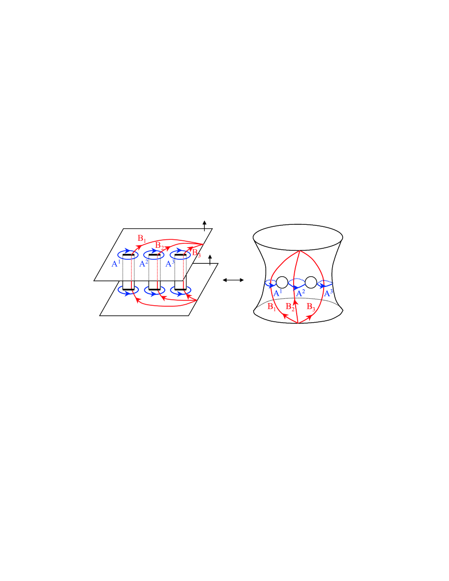
Figure 1: A symplectic choice of compact $A$- and non-compact $B$-cycles for $n=3$. Note that the orientation of the two planes on the left-hand side is chosen such that both normal vectors point to the top. This is why the orientation of the $A$-cycles is different on the two planes. To go from the representation of the Riemann surface on the left to the one on the right one has to flip the upper plane.

There are various symplectic bases of this relative homology group. One such basis is $\{A^{i},B_{j}\}$, with $i,j=1,\ldots n$, where the one-cycle $A^{i}$ runs around the $i$-th cut and the relative one-cycles $B_{j}$ are all non-compact and run from $Q^{\prime}$ through the $j$-th cut to $Q$. This is the choice of cycles used in [11] and it is shown in Fig.1.

Another useful symplectic basis is the set $\{\alpha^{i},\beta_{j},\hat{\alpha},\hat{\beta}\}$, with ${\hat{g}}=n-1$ compact cycles $\alpha^{i}$ and ${\hat{g}}=n-1$ compact cycles $\beta_{i}$, with intersection numbers $\alpha^{i}\cap\beta_{j}=\delta^{i}_{j}$, together with one compact cycle $\hat{\alpha}$ and one non-compact cycle $\hat{\beta}$, with $\hat{\alpha}\cap\hat{\beta}=1$, see Fig.2. Note that although these bases are equivalent, since one can be obtained from the other by a symplectic transformation, the second basis is much more useful for our purpose. This is because it contains only one non-compact cycle and the new features coming from the non-compactness of the space should be contained entirely in the corresponding integral. Finally, we take $\Gamma_{A^{i}},\Gamma_{B_{j}}$ to be the $S^{2}$-fibrations over $A^{i},B_{j}$ and $\Gamma_{\alpha^{i}},\Gamma_{\beta_{j}}$ $S^{2}$-fibrations over $\alpha^{i},\beta_{j}$.

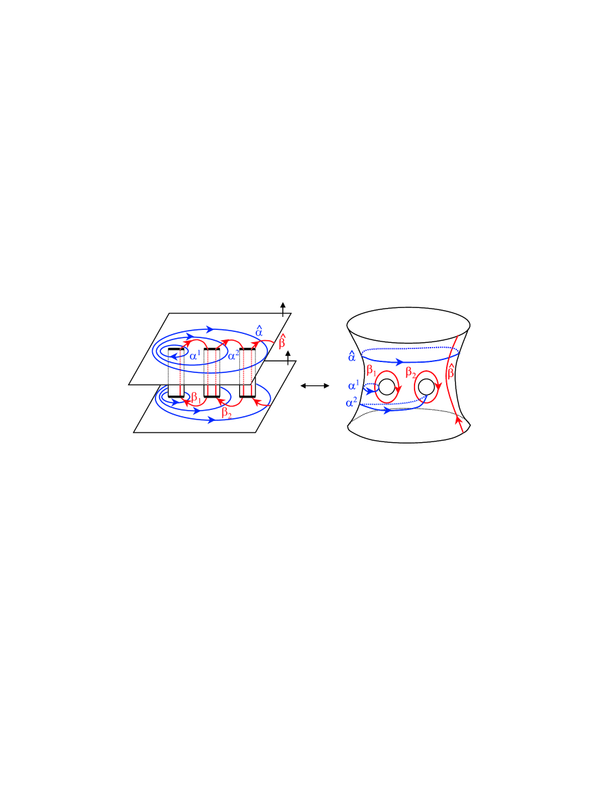
Figure 2: A symplectic set of cycles containing only one non-compact cycle $\hat{\beta}$. The cycle $\alpha^{i}$ surrounds $i$ of the cuts, whereas the cycle $\beta_{i}$ runs from cut $i$ to cut $i+1$ on the upper sheet and from cut $i+1$ to cut $i$ on the lower one. As before one has to flip the upper plane to find the representation of the surface on the right.

So the problem effectively reduces to calculating the integrals

$$\int_{\Gamma_{\gamma}}\Omega=-i\pi\int_{\gamma}\zeta\ \ \ \mbox{for}\ \ \ \gamma\in\{\alpha^{i},\beta_{j},\hat{\alpha},\hat{\beta}\}\ .$$ (2.6)

For ${\hat{g}}=1$ they can be reduced to various combinations of elliptic integrals of the three kinds.

As we mentioned already, we expect new features to be contained in the integral $\int_{\hat{\beta}}\zeta$, where $\hat{\beta}$ runs from $Q^{\prime}$ on the lower sheet to $Q$ on the upper one. Indeed, it is easy to see that this integral is divergent. It will be part of our task to understand and properly treat this divergence. As usual, we will regulate the integral and we have to make sure that physical quantities do not depend on the regulator and remain finite once the regulator is removed. Usually this is achieved by simply discarding the divergent part. Instead, we want to give a more intrinsic geometric prescription that will be similar to standard procedures in relative cohomology. To render the integral finite we simply cut out two “small” discs around the points $Q,Q^{\prime}$. If $x,x^{\prime}$ are coordinates on the upper and lower sheet respectively, we restrict ourselves to $|x|\leq\Lambda_{0}$, $|x^{\prime}|\leq\Lambda_{0}$, $\Lambda_{0}\in\mathbb{R}$. Furthermore we take the cycle $\hat{\beta}$ to run from the point $\Lambda_{0}^{\prime}$ on the real axis of the lower sheet to $\Lambda_{0}$ on the real axis of the upper sheet. (Actually we could take $\Lambda_{0}$ and $\Lambda_{0}^{\prime}$ to be complex. We will come back to this point later on.)

3 Holomorphic Matrix Models and Special Geometry

Our goal is to relate the integrals (2.6) to the prepotential $\mathcal{F}_{0}$. It turns out that in order to address this problem it is useful to perform calculations in the matrix model that corresponds to our local Calabi-Yau manifold. Indeed, the analysis of Dijkgraaf and Vafa tells us [15] that one should identify the prepotential and the planar limit of the free energy of the holomorphic matrix model with potential $W(x)$. Therefore, our goal will be to find the special geometry relation in the holomorphic matrix model and to see how the integrals (2.6) over the cycles $\alpha^{i},\beta_{j},\hat{\alpha},\hat{\beta}$ are related to the planar limit of the free energy.
One should note, however, that in the matrix model the filling fractions $S_{i}$, related to the integrals over the $A$-cycles, are manifestly real, even though $W(x)$ has arbitrary complex coefficients. So, strictly speaking, the matrix model does not explore the full moduli space of the Calabi-Yau manifold. Nevertheless, we will see that all relevant formulae can be immediately continued to complex values of the $S_{i}$ and, in particular, the special geometry relations continue to be true.

3.1 The Holomorphic Matrix Model

The proper definition of the holomorphic matrix model is somewhat more subtle than the one of the hermitian matrix model. Many of these subtleties were nicely addressed in [17] and we will briefly review them here. The usual identification of the planar limit with the saddle point approximation involves even more subtleties which we will have to clarify in this subsection. Particular attention is paid to the dependence of the free energy on the various parameters.

3.1.1 The partition function and convergence properties

We begin by defining the partition function of the holomorphic one-matrix model following [17]. In order to do so, one chooses a smooth path $\gamma:\mathbb{R}\rightarrow\mathbb{C}$ without self-intersection, such that $\dot{\gamma}(u)\neq 0\ \forall u\in\mathbb{R}$ and $|\gamma(u)|\rightarrow\infty$ for $u\rightarrow\pm\infty$. Consider the ensemble $\Gamma(\gamma)$ of $\hat{N}\times\hat{N}$ complex matrices $M$ with spectrum spec$(M)=\{\lambda_{1},\ldots\lambda_{\hat{N}}\}$ in $\gamma$ and distinct eigenvalues,

$$\Gamma(\gamma):=\{M\in\mathbb{C}^{\hat{N}\times\hat{N}}:\mbox{spec}(M)\subset\gamma,\ \mbox{all}\ \lambda_{m}\ \mbox{distinct}\}\ .$$ (3.1)

The holomorphic measure on $\mathbb{C}^{\hat{N}\times\hat{N}}$ is just ${\rm d}M\equiv\wedge_{p,q}{\rm d}M_{pq}$ with some appropriate sign convention. The (super-)potential is

$$W(x):=g_{0}+\sum_{k=1}^{n+1}{g_{k}\over k}x^{k},\ \ \ g_{n+1}=1\ .$$ (3.2)

Without loss of generality we have chosen $g_{n+1}=1$. The only restriction for the other complex parameters $\{g_{k}\}_{k=0,\ldots n}$, collectively denoted by $g$, comes from the fact that the $n$ critical points $\mu_{i}$ of $W$ should not be degenerate, i.e. $W^{\prime\prime}(\mu_{i})\neq 0$ if $W^{\prime}(x)=\prod_{i=1}^{n}(x-\mu_{i})$. Then the partition function of the holomorphic one-matrix model is

$$Z(\Gamma(\gamma),g,g_{s},\hat{N}):=C_{\hat{N}}\int_{\Gamma(\gamma)}{\rm d}M\ \exp\left(-{1\over g_{s}}\,{\rm tr}\,W(M)\right),$$ (3.3)

where $g_{s}$ is a positive coupling constant and $C_{\hat{N}}$ is some normalisation factor. To avoid cluttering the notation we will omit the dependence on $\gamma$ and $g$ and write $Z(g_{s},\hat{N}):=Z(\Gamma(\gamma),g,g_{s},\hat{N})$. As usual one diagonalises $M$ and performs the integral over the diagonalising matrices. The constant $C_{\hat{N}}$ is chosen in such a way that one arrives at

$$Z(g_{s},\hat{N})={1\over{\hat{N}!}}\int_{\gamma}{\rm d}\lambda_{1}\ldots\int_{\gamma}{\rm d}\lambda_{\hat{N}}\exp\left({-\hat{N}^{2}S(g_{s},\hat{N};\lambda_{m})}\right)=:e^{-F(g_{s},\hat{N})}\ ,$$ (3.4)

where

$$S(g_{s},\hat{N};\lambda_{m})={1\over\hat{N}^{2}g_{s}}\sum_{m=1}^{\hat{N}}W(\lambda_{m})-{1\over\hat{N}^{2}}\sum_{p\neq q}\ln(\lambda_{p}-\lambda_{q})\ .$$ (3.5)

See [17] for more details.

The convergence of the $\lambda_{m}$ integrals depends on the polynomial $W$ and the choice of the path $\gamma$. For given $W$ the asymptotic part of the complex plane ($|x|$ large) can be divided into convergence domains $G_{k}^{(c)}$ and divergence domains $G_{k}^{(d)}$, $k=1,\ldots n+1$, where $e^{-{1\over g_{s}}W(x)}$ converges, respectively diverges as $|x|\rightarrow\infty$. The path $\gamma$ has to be chosen [17] to go from some convergence domain $G_{k}^{(c)}$ to some other $G_{l}^{(c)}$, with $k\neq l$; call such a path $\gamma_{kl}$, see Fig.3.

Figure 3: Example of convergence and divergence domains for $n=2$ and a possible choice of $\gamma_{21}$. Because of holomorphicity the path can be deformed without changing the partition function, for instance one could use the path $\tilde{\gamma}_{21}$ instead.

Then the value of the partition function depends only on the pair $(k,l)$ and, because of holomorphicity, is not sensitive to deformations of $\gamma_{kl}$. In particular, instead of $\gamma_{kl}$ we can make the equivalent choice

$$\tilde{\gamma}_{kl}=\gamma_{p_{1}p_{2}}\cup\gamma_{p_{2}p_{3}}\cup\ldots\cup\gamma_{p_{n-1}p_{n}}\cup\gamma_{p_{n}p_{n+1}}\ \ \ \mbox{with}\ p_{1}=k,\ p_{n+1}=l,$$ (3.6)

as shown in Fig.3. Here we split the path into $n$ components, each component running from one convergence sector to another. Again, due to holomorphicity we can choose the decomposition in such a way that every component $\gamma_{p_{i}p_{i+1}}$ runs through one of the $n$ critical points of $W$ in $\mathbb{C}$, or at least comes close to it. This choice of $\tilde{\gamma}_{kl}$ will turn out to be very useful to understand the saddle point approximation discussed below. Hence, the partition function and the free energy depend on the pair $(k,l),g,g_{s}$ and $\hat{N}$. Of course, one can always relate the partition function for arbitrary $(k,l)$ to one with $(k^{\prime},1)$, $k^{\prime}=k-l+1$ mod $n$, and redefined coupling constants $g$.

3.1.2 Matrix model technology

Next, we need to recall some standard technology adapted to the holomorphic matrix model. We first assume that the path $\gamma$ consists of a single connected piece. The case (3.6) will be discussed later on. Let $s$ be the length coordinate of the path $\gamma$, centered at some point on $\gamma$, and let $\lambda(s)$ denote the parameterisation of $\gamma$ with respect to this coordinate. Then, for an eigenvalue $\lambda_{m}$ on $\gamma$, one has $\lambda_{m}=\lambda(s_{m})$ and the partition function can be rewritten as

$$Z(g_{s},\hat{N})={1\over{\hat{N}!}}\int_{\mathbb{R}}{\rm d}s_{1}\ldots\int_{\mathbb{R}}{\rm d}s_{\hat{N}}\prod_{l=1}^{\hat{N}}\dot{\lambda}(s_{l})\exp\left(-\hat{N}^{2}S(g_{s},\hat{N};\lambda(s_{m}))\right)\ .$$ (3.7)

The spectral density is defined as

$$\rho(s,s_{m}):={1\over\hat{N}}\sum_{m=1}^{\hat{N}}\delta(s-s_{m})\ ,$$ (3.8)

so that $\rho$ is normalised to one, $\int_{-\infty}^{\infty}\rho(s,s_{m}){\rm d}s=1$. The normalised trace of the resolvent of the matrix $M$ is given by

$$\omega(x,s_{m}):={1\over\hat{N}}\,{\rm tr}\,{1\over{x-M}}={1\over\hat{N}}\sum_{m=1}^{\hat{N}}{1\over{x-\lambda(s_{m})}}=\int{\rm d}s{\rho(s,s_{m})\over{x-\lambda(s)}}\ ,$$ (3.9)

for $x\in\mathbb{C}$. Following [17] we decompose the complex plane into domains $D_{i}$, $i\in\{1,\ldots,n\}$, with mutually disjoint interior, $(\cup_{i}\overline{D}_{i}=\mathbb{C},\ \ D_{i}\cap D_{j}=\emptyset\ \ \mbox{for}\ i\neq j)$. These domains are chosen in such a way that $\gamma$ intersects each $\overline{D}_{i}$ along a single line segment $\Delta_{i}$, and $\cup_{i}\Delta_{i}=\gamma$. Furthermore, $\mu_{i}$, the $i$-th critical point of $W$, should lie in the interior of $D_{i}$. One defines

$$\chi_{i}(M):=\int_{\partial D_{i}}{{\rm d}x\over 2\pi i}{1\over{x-M}}\ ,$$ (3.10)

(which projects on the space spanned by the eigenvectors of $M$ whose eigenvalues lie in $D_{i}$), and the filling fractions $\tilde{\sigma}_{i}(\lambda_{m}):={1\over\hat{N}}\,{\rm tr}\,\chi_{i}(M)$ and

$$\sigma_{i}(s_{m}):=\tilde{\sigma}_{i}(\lambda(s_{m}))=\int{\rm d}s\ \rho(s,s_{m})\chi_{i}(\lambda(s))=\int_{\partial D_{i}}{{\rm d}x\over 2\pi i}\ \omega(x,s_{m})\ ,$$ (3.11)

(which count the eigenvalues in the domain $D_{i}$, times $1/\hat{N}$). Obviously

$$\sum_{i=1}^{n}\sigma_{i}(s_{m})=1\ .$$ (3.12)

One can apply standard methods (e.g. the ones of [20]) to derive the loop equations of the holomorphic matrix model,

$$\langle\omega(x,s_{m})^{2}\rangle-{1\over t}W^{\prime}(x)\langle\omega(x,s_{m})\rangle-{1\over 4t^{2}}\langle f(x,s_{m})\rangle=0\ .$$ (3.13)

Here

$$t=g_{s}\hat{N}$$ (3.14)

is the quantity that will be held fixed in the planar limit below,

$$f(x,s_{m}):=-{4t\over{\hat{N}}}\sum_{m=1}^{\hat{N}}{{W^{\prime}(x)-W^{\prime}(\lambda(s_{m}))}\over{x-\lambda(s_{m})}}=-4t\int{\rm d}s\ \rho(s,s_{m}){{W^{\prime}(x)-W^{\prime}(\lambda(s))}\over{x-\lambda(s)}}\ ,$$ (3.15)

and the expectation value is defined for a $h(\lambda_{m})=h(\lambda(s_{m}))$ as usual:

$$\langle h(\lambda_{m})\rangle:={1\over Z(g_{s},\hat{N})}\cdot{1\over\hat{N}!}\int_{\gamma}{\rm d}\lambda_{1}\ldots\int_{\gamma}{\rm d}\lambda_{\hat{N}}\ h(\lambda_{m})\exp\left(-\hat{N}^{2}S(g_{s},\hat{N};\lambda_{m})\right)\ .$$ (3.16)

It will be useful to define an effective action as

$$S_{eff}(g_{s},\hat{N};s_{m}):=S(g_{s},\hat{N};\lambda(s_{m}))-{1\over\hat{N}^{2}}\sum_{m=1}^{\hat{N}}\ln(\dot{\lambda}(s_{m}))$$

$$=\int{\rm d}s\ \rho(s;s_{m})\left({1\over t}W(\lambda(s))-{1\over{\hat{N}}}\ln(\dot{\lambda}(s))-\mathcal{P}\int{\rm d}s^{\prime}\ \rho(s^{\prime};s_{p})\ln(\lambda(s)-\lambda(s^{\prime}))\right)\ \ \ \ \ \ \ \ \ \$$ (3.17)

so that

$$Z(g_{s},\hat{N})={1\over{\hat{N}!}}\int{\rm d}s_{1}\ldots\int{\rm d}s_{\hat{N}}\ \exp\left(-\hat{N}^{2}S_{eff}(g_{s},\hat{N};s_{m})\right)\ .$$ (3.18)

Note that the principal value is defined as

$$\mathcal{P}\ \ln\left(\lambda(s)-\lambda(s^{\prime})\right)={1\over 2}\lim_{\epsilon\rightarrow 0}\left[\ln\left(\lambda(s)-\lambda(s^{\prime})+i\epsilon\dot{\lambda}(s)\right)+\ln\left(\lambda(s)-\lambda(s^{\prime})-i\epsilon\dot{\lambda}(s)\right)\right]\ .$$ (3.19)

The equations of motion corresponding to this effective action, ${\delta S_{eff}\over\delta s_{m}}=0$, read

$${1\over t}W^{\prime}(\lambda(s_{m}))={2\over{\hat{N}}}\sum_{p=1,\ p\neq m}^{\hat{N}}{1\over{\lambda(s_{m})-\lambda(s_{p})}}+{1\over{\hat{N}}}{\ddot{\lambda}(s_{m})\over\dot{\lambda}(s_{m})^{2}}\ .$$ (3.20)

Using these equations of motion one can show that

$$\omega(x,s_{m})^{2}-{1\over t}W^{\prime}(x)\omega(x,s_{m})-{1\over 4t^{2}}f(x,s_{m})+$$

$$+{1\over\hat{N}}{{\rm d}\over{\rm d}x}\omega(x,s_{m})+{1\over\hat{N}^{2}}\sum_{m=1}^{\hat{N}}{\ddot{\lambda}(s_{m})\over\dot{\lambda}(s_{m})^{2}}{1\over{x-\lambda(s_{m})}}=0\ .$$ (3.21)

Solutions of the equations of motion
Note that in general the effective action is a complex function of the real $s_{m}$. Hence, in general, i.e. for a generic path $\gamma_{kl}$ with parameterisation $\lambda(s)$, there will be no solution to (3.20). One clearly expects that the existence of solutions must constrain the path $\lambda(s)$ appropriately. Let us study this in more detail.
Recall that we defined the domains $D_{i}$ in such a way that $\mu_{i}\subset D_{i}$. Let $\hat{N}_{i}$ be the number of eigenvalues $\lambda(s_{m})$ which lie in the domain $D_{i}$, so that $\sum_{i=1}^{n}\hat{N}_{i}=\hat{N}$, and denote them by $\lambda(s_{a}^{(i)})$, $a\in\{1,\ldots\hat{N}_{i}\}$.
Solving the equations of motion in general is a formidable problem. To get a good idea, however, recall the picture of $\hat{N}_{i}$ fermions filled into the $i$-th “minimum” of ${1\over t}W$ [21]. For small $t$ the potential is deep and the fermions are located not too far from the minimum, in other words all the eigenvalues are close to $\mu_{i}$. To be more precise consider (3.20) and drop the last term, an approximation that will be justified momentarily. Let us take $t$ to be small and look for solutions $\lambda(s_{a}^{(i)})=\mu_{i}+\sqrt{t}\delta\lambda_{a}^{(i)}$, where $\delta\lambda_{a}^{(i)}$ is of order one. So, we assume that the eigenvalues $\lambda(s_{a}^{(i)})$ are not too far from the critical point $\mu_{i}$. Then the equation reads

$$W^{\prime\prime}(\mu_{i})\delta\lambda_{a}^{(i)}={2\over\hat{N}}\sum_{b=1,\ b\neq a}^{\hat{N}_{i}}{1\over{\delta\lambda^{(i)}_{a}-\delta\lambda_{b}^{(i)}}}+o(\sqrt{t})\ ,$$ (3.22)

so we effectively reduced the problem to finding the solution for $n$ distinct quadratic potentials. If we set $z_{a}:=\sqrt{\hat{N}W^{\prime\prime}(\mu_{i})\over 2}\delta\lambda_{a}^{(i)}$ and neglect the $o(\sqrt{t})$-terms this gives

$$z_{a}=\sum_{b=1,\ b\neq a}^{\hat{N}_{i}}{1\over{z_{a}-z_{b}}}\ ,$$ (3.23)

which can be solved explicitly for small $\hat{N}_{i}$. It is obvious that $\sum_{a=1}^{\hat{N}_{i}}z_{a}=0$, and one finds that there is a unique solution (up to permutations) with the $z_{a}$ symmetrically distributed around 0 on the real axis. This justifies a posteriori that we really can neglect the term proportional to the second derivative of $\lambda(s)$, at least to leading order. Furthermore, setting $W^{\prime\prime}(\mu_{i})=|W^{\prime\prime}(\mu_{i})|e^{i\phi_{i}}$ one finds that the $\lambda(s_{a}^{i})$ sit on a tilted line segment around $\mu_{i}$ where the angle of the tilt is given by $-\phi_{i}/2$. This means for example that for a potential with $W^{\prime}(x)=x(x-1)(x+1)$ the eigenvalues are distributed on the real axis around $\pm 1$ and on the imaginary axis around 0. Note further that, in general, the reality of $z_{a}$ implies that ${W^{\prime\prime}(\mu_{i})\over 2}\left({\delta\lambda^{(i)}_{a}}\right)^{2}>0$ which tells us that, close to $\mu_{i}$, $W(\lambda(s))-W(\mu_{i})$ is real with a minimum at $\lambda(s)=\mu_{i}$.
So we have found that the path $\gamma_{kl}$ has to go through the critical points $\mu_{i}$ with a tangent direction fixed by the phase of the second derivative of $W$. On the other hand, we know that the partition function does not depend on the form of the path $\gamma_{kl}$. Of course, there is no contradiction: if one wants to compute the partition function from a saddle point expansion, as we will do below, and as is implicit in the planar limit, one has to make sure that one expands around solutions of (3.20) and the existence of these solutions imposes conditions on how to choose the path $\gamma_{kl}$. From now on we will assume that the path is chosen in such a way that it satisfies all these constraints. Furthermore, for later purposes it will be useful to use the path $\tilde{\gamma}_{kl}$ of (3.6) chosen such that its part $\gamma_{p_{i}p_{i+1}}$ goes through all $\hat{N}_{i}$ solutions $\lambda_{a}^{(i)}$, $a=1,\ldots\hat{N}_{i}$, and lies entirely in $D_{i}$, see Fig.4.

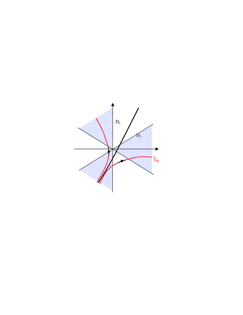
Figure 4: For the cubic potential of Fig.3 we show the choice of the domains $D_{1}$ and $D_{2}$ and of the path $\tilde{\gamma}_{21}$ with respect to the two critical points, as well as the cuts that form around these points.

It is natural to assume that these properties together with the uniqueness of the solution (up to permutations) extend to higher numbers of $\hat{N}_{i}$ as well. Of course once one goes beyond the leading order in $\sqrt{t}$ the eigenvalues are no longer distributed on a straight line, but on a line segment that is bent in general and that might or might not pass through $\mu_{i}$.

The large $\hat{N}$ limit
We are interested in the large $\hat{N}$ limit of the matrix model free energy. It is well known that the expectation values of the relevant quantities like $\rho$ or $\omega$ have expansions of the form

$$\langle\rho(s,s_{m})\rangle=\sum_{I=0}^{\infty}\rho_{I}(s)\hat{N}^{-I}\ \ \ ,\ \ \ \langle\omega(x,s_{m})\rangle=\sum_{I=0}^{\infty}\omega_{I}(x)\hat{N}^{-I}\ .$$ (3.24)

Clearly, $\omega_{0}(x)$ is related to $\rho_{0}(s)$ by the large $\hat{N}$ limit of (3.9), namely

$$\omega_{0}(x)=\int{\rm d}s{\rho_{0}(s)\over{x-\lambda(s)}}\ .$$ (3.25)

We saw already that an eigenvalue ensemble that solves the equations of motion is distributed along line segments around the critical points $\mu_{i}$. In the limit $\hat{N}\rightarrow\infty$ this will turn into a continuous distribution on the segments $\mathcal{C}_{i}$, through or close to the critical points of $W$. Then $\rho_{0}(s)$ has support only on these $\mathcal{C}_{i}$ and $\omega_{0}(x)$ is analytic in $\mathbb{C}$ with cuts $\mathcal{C}_{i}$. Conversely, $\rho_{0}(s)$ is given by the discontinuity of $\omega_{0}(x)$ across its cuts:

$$\rho_{0}(s):=\dot{\lambda}(s)\lim_{\epsilon\rightarrow 0}{1\over 2\pi i}[\omega_{0}(\lambda(s)-i\epsilon\dot{\lambda}(s))-\omega_{0}(\lambda(s)+i\epsilon\dot{\lambda}(s))]\ .$$ (3.26)

The planar limit we are interested in is $\hat{N}\rightarrow\infty$, $g_{s}\rightarrow 0$ with $t=g_{s}\hat{N}$ held fixed. Hence we rewrite all $\hat{N}$ dependence as a $g_{s}$ dependence and consider the limit $g_{s}\rightarrow 0$. Then, the equation of motion (3.20) reduces to

$${1\over t}W^{\prime}(\lambda(s))=2\mathcal{P}\int{\rm d}s^{\prime}\ {\rho_{0}(s^{\prime})\over{\lambda(s)-\lambda(s^{\prime})}}\ .$$ (3.27)

Note that this equation is only valid for those $s$ where eigenvalues exist, i.e. where $\rho_{0}(s)\neq 0$. In principle one can use this equation to compute the planar eigenvalue distribution $\rho_{0}(s)$ for given $W^{\prime}$.

Riemann surfaces and planar solutions
The leading term in the expansion (3.24) for $\langle\omega(s,s_{m})\rangle$ can be calculated from a saddle point approximation, where the $\{s_{m}\}$ are given by a solution $\{s_{m}^{*}\}$ of (3.20): $\omega_{0}(x)=\omega(x;s_{m}^{*})$. This is true for all “microscopic” operators, i.e. operators that do not modify the saddle point equations (3.20). (Things would be different for “macroscopic”operators like $e^{\hat{N}\sum_{p=1}^{\hat{N}}V(\lambda_{p})}$.) In particular, this shows that expectation values factorise in the large $\hat{N}$ limit, and the loop equation (3.13) reduces to the algebraic equation

$$\omega_{0}(x)^{2}-{1\over t}W^{\prime}(x)\omega_{0}(x)-{1\over 4t^{2}}f_{0}(x)=0\ ,$$ (3.28)

where

$$f_{0}(x)=-4t\int{\rm d}s\ \rho_{0}(s){{W^{\prime}(x)-W^{\prime}(\lambda(s))}\over{x-\lambda(s)}}$$ (3.29)

is a polynomial of degree $n-1$ with leading coefficient $-4t$. Note that this coincides with the planar limit of equation (3.1.2). If we define

$$y_{0}(x):=W^{\prime}(x)-{2t}\omega_{0}(x)\ ,$$ (3.30)

then $y_{0}$ is one of the branches of the algebraic curve

$$y^{2}=W^{\prime}(x)^{2}+f_{0}(x)\ ,$$ (3.31)

as can be seen from (3.28). On this curve we use the same conventions as in section 2, i.e. $y_{0}(x)$ is defined on the upper sheet and cycles and orientations are chosen as in Fig.1 and Fig.2.

Solving a matrix model in the planar limit means to find a normalised, real, non-negative $\rho_{0}(s)$ and a path $\tilde{\gamma}_{kl}$ which satisfy (3.25), (3.27) and (3.28/3.29) for a given potential $W(z)$ and a given asymptotics $(k,l)$ of $\gamma$.

Interestingly, for any algebraic curve (3.31) there is a contour $\tilde{\gamma}_{kl}$ supporting a formal solution of the matrix model in the planar limit. To construct it start from an arbitrary polynomial $f_{0}(x)$ or order $n-1$, with leading coefficient $-4t$, which is given together with the potential $W(x)$ of order $n+1$. The corresponding Riemann surface is given by (3.31), and we denote its branch points by $a_{i}^{\pm}$ and choose branch-cuts $\mathcal{C}_{i}$ between them. We can read off the two solutions $y_{0}$ and $y_{1}=-y_{0}$ from (3.31), where we take $y_{0}$ to be the one with a behaviour $y_{0}\stackrel{{\scriptstyle x\rightarrow\infty}}{{\rightarrow}}+W^{\prime}(x)$. $\omega_{0}(x)$ is defined as in (3.30) and we choose a path $\tilde{\gamma}_{kl}$ such that $\mathcal{C}_{i}\subset\tilde{\gamma}_{kl}$ for all $i$. Then the formal planar spectral density satisfying all the requirements can be determined from (3.26) (see [17]). However, in general, this will lead to a complex distribution $\rho_{0}(s)$. This can be understood from the fact the we constructed $\rho_{0}(s)$ from a completely arbitrary hyperelliptic Riemann surface. However, in the matrix model the algebraic curve (3.31) is not general, but the coefficients $\alpha_{k}$ of $f_{0}(x)$ are constraint. This can be seen by computing the filling fractions

$$\nu_{i}^{*}:=\langle\sigma_{i}(s_{m})\rangle={1\over 2\pi i}\int_{\partial D_{i}}\omega_{0}(x){\rm d}x={1\over 4\pi it}\int_{A^{i}}y_{0}(x){\rm d}x=\int_{\gamma^{-1}(\mathcal{C}_{i})}\rho_{0}(s){\rm d}s\ ,$$ (3.32)

which must be real and non-negative. Here we used the fact that the $D_{i}$ were chosen such that $\gamma_{p_{i}p_{i+1}}\subset D_{i}$ and therefore $\mathcal{C}_{i}\subset D_{i}$, so for $D_{i}$ on the upper plane, $\partial D_{i}$ is homotopic to $-A^{i}$. Hence, ${\rm Im}\left(i\int_{A^{i}}y(x){\rm d}x\right)=0$ which constrains the $\alpha_{k}$. We conclude that to construct distributions $\rho_{0}(s)$ that are relevant for the matrix model one can proceed along the lines described above, but one has to impose the additional constraint that $\rho_{0}(s)$ is real. As for finite $\hat{N}$, this will impose conditions on the possible paths $\tilde{\gamma}_{kl}$ supporting the eigenvalue distributions.

To see this, we assume that the coefficients $\alpha_{k}$ in $f_{0}(x)$ are small, so that the lengths of the cuts are small compared to the distances between the different critical points: $|a_{i}^{+}-a_{i}^{-}|\ll|\mu_{i}-\mu_{j}|$. Then in first approximation the cuts are straight line segments between $a_{i}^{+}$ and $a_{i}^{-}$. For $x$ close to the cut $\mathcal{C}_{i}$ we have $y^{2}\approx(x-a_{i}^{+})(x-a_{i}^{-})\prod_{j\neq i}(\mu_{i}-\mu_{j})^{2}=(x-a_{i}^{+})(x-a_{i}^{-})(W^{\prime\prime}(\mu_{i}))^{2}$. If we set $W^{\prime\prime}(\mu_{i})=|W^{\prime\prime}(\mu_{i})|e^{i\phi_{i}}$ and $a_{i}^{+}-a_{i}^{-}=r_{i}e^{i\psi_{i}}$, then, on the cut $\mathcal{C}_{i}$, the path $\gamma$ is parameterised by $\lambda(s)={a_{i}^{+}-a_{i}^{-}\over|a_{i}^{+}-a_{i}^{-}|}s=se^{i\psi_{i}}$, and we find from (3.26)

$$\rho_{0}(s) = {1\over 2\pi t}\sqrt{|\lambda(s)-a_{1}^{+}|}\sqrt{|\lambda(s)-a_{1}^{-}|}\ |W^{\prime\prime}(\mu_{i})|e^{i(\phi_{i}+2\psi_{i})}$$ (3.33)

$$= {1\over 2\pi t}\sqrt{|\lambda(s)-a_{1}^{+}|}\sqrt{|\lambda(s)-a_{1}^{-}|}\ W^{\prime\prime}(\mu_{i})(\dot{\lambda}(s))^{2}\ .$$

So reality and positivity of $\rho_{0}(s)$ lead to conditions on the orientation of the cuts in the complex plane, i.e. on the path $\gamma$:

$$\psi_{i}=-{\phi_{i}/2}\ \ \ \ \ \ ,\ \ \ \ \ W^{\prime\prime}(\mu_{i})(\dot{\lambda}(s))^{2}>0\ .$$ (3.34)

These are precisely the conditions we already derived for the case of finite $\hat{N}$. We see that the two approaches are consistent and, for given $W$ and fixed $\hat{N}_{i}$ respectively $\nu_{i}^{*}$, lead to a unique solution $\{\lambda(s),\rho_{0}(s)\}$ with real and positive eigenvalue distribution. Note again that the requirement of reality and positivity of $\rho_{0}(s)$ constrains the phases of $a_{i}^{+}-a_{i}^{-}$ and hence the coefficients $\alpha_{k}$ of $f_{0}(x)$.

3.1.3 The saddle point approximation for the partition function

Recall that our goal is to find a relation between the planar limit ($t=g_{s}\hat{N}$ fixed, $g_{s}\rightarrow 0$) of the free energy of the matrix model and the period integrals of $y(x){\rm d}x$ on the corresponding Riemann curve. Since the standard planar free energy $F_{0}(t)$ depends on $t$ only it cannot appear in relations like (LABEL:SG), and one has to introduce a set of sources $J_{i}$ to have a free energy that depends on more variables. In this subsection we evaluate this source dependent free energy and its Legendre transform $\mathcal{F}_{0}(t,S)$ in the planar limit using a saddle point expansion.

We start by coupling sources to the filling fractions,

$$Z(g_{s},\hat{N},J) := {1\over{\hat{N}!}}\int_{\gamma}{\rm d}\lambda_{1}\ldots\int_{\gamma}{\rm d}\lambda_{\hat{N}}\exp\left(-\hat{N}^{2}S(g_{s},\hat{N};\lambda_{m})-{\hat{N}\over g_{s}}\sum_{i=1}^{n-1}J_{i}\tilde{\sigma}_{i}(\lambda_{m})\right)$$ (3.35)

$$= \exp\left(-F(g_{s},\hat{N},J)\right)\ .$$

where $J:=\{J_{1},\ldots,J_{n-1}\}$. Note that because of the constraint $\sum_{i=1}^{n}\tilde{\sigma}_{i}(\lambda_{m})=1$, $\tilde{\sigma}_{n}(\lambda_{m})$ is not an independent quantity and we can have only $n-1$ sources. This differs from the treatment in [17] and has important consequences, as we will see in the next section. We want to evaluate this partition function for $\hat{N}\rightarrow\infty$, $t=g_{s}\hat{N}$ fixed, from a saddle point approximation. We therefore use the path $\tilde{\gamma}_{kl}$ from (3.6) that was chosen in such a way that the equation of motion (3.20) has solutions $s_{m}^{*}$ and, for large $\hat{N}$, $\mathcal{C}_{i}\subset\gamma_{p_{i}p_{i+1}}$. It is only then that the saddle point expansion converges and makes sense. Obviously then each integral $\int_{\gamma}{\rm d}\lambda_{m}$ splits into a sum $\sum_{i=1}^{n}\int_{\gamma_{p_{i}p_{i+1}}}{\rm d}\lambda_{m}$. Let $s^{(i)}\in\mathbb{R}$ be the length coordinate on $\gamma_{p_{i}p_{i+1}}$, so that $s^{(i)}$ runs over all of $\mathbb{R}$. Furthermore, $\tilde{\sigma}_{i}(\lambda_{m})$ only depends on the number $\hat{N}_{i}$ of eigenvalues in $\tilde{\gamma}_{kl}\cap D_{i}=\gamma_{p_{i}p_{i+1}}$. Then the partition function (3.35) is a sum of contributions with fixed $\hat{N}_{i}$ and we rewrite is as

$$Z(g_{s},N,J)=\sum_{\stackrel{{\scriptstyle\sum_{i}\hat{N}_{i}=\hat{N}}}{{\hat{N}_{1},\ldots,\hat{N}_{n}}}}Z(g_{s},\hat{N},\hat{N}_{i})e^{-{1\over g_{s}}\sum_{i=1}^{n-1}J_{i}\hat{N}_{i}}\ ,$$ (3.36)

where now

$$Z(g_{s},\hat{N},\hat{N}_{i})=$$

$$={1\over\hat{N}_{1}\ldots\hat{N}_{n}!}\int_{\gamma_{p_{1}p_{2}}}{\rm d}\lambda^{(1)}_{1}\ldots\int_{\gamma_{p_{1}p_{2}}}{\rm d}\lambda^{(1)}_{\hat{N}_{1}}\ldots\int_{\gamma_{p_{n}p_{n+1}}}{\rm d}\lambda^{(n)}_{1}\ldots\int_{\gamma_{p_{n}p_{n+1}}}{\rm d}\lambda^{(n)}_{\hat{N}_{n}}\exp\left(-{t^{2}\over g_{s}^{2}}S(g_{s},t;\lambda_{k}^{(i)})\right)$$

$$=:\exp\left(\tilde{\mathcal{F}}(g_{s},t,\hat{N}_{i})\right)$$ (3.37)

is the partition function with the additional constraint that precisely $\hat{N}_{i}$ eigenvalues lie on $\gamma_{p_{i}p_{i+1}}$. Note that it depends on $g_{s},t=g_{s}\hat{N}$ and $\hat{N}_{1},\ldots\hat{N}_{n-1}$ only, as $\sum_{i=1}^{n}\hat{N}_{i}=\hat{N}$. Now that these numbers have been fixed, there is precisely one solution to the equations of motion, i.e. a unique saddle-point configuration, up to permutations of the eigenvalues, on each $\gamma_{p_{i}p_{i+1}}$. These permutations just generate a factor $\prod_{i}\hat{N}_{i}!$ which cancels the corresponding factor in front of the integral. As discussed above, it is important that we have chosen the $\gamma_{p_{i}p_{i+1}}$ to support this saddle point configuration close to the critical point $\mu_{i}$ of $W$. Moreover, since $\gamma_{p_{i}p_{i+1}}$ runs from one convergence sector to another and by (3.34) the saddle point really is dominant (stable), the “one-loop” and other higher order contributions are indeed subleading as $g_{s}\rightarrow 0$ with $t=g_{s}\hat{N}$ fixed. This is why we had to be so careful about the choice of our path $\gamma$ as being composed of $n$ pieces $\gamma_{p_{i}p_{i+1}}$. In the planar limit $\nu_{i}:={\hat{N}_{i}\over\hat{N}}$ is finite, and $\tilde{\mathcal{F}}(g_{s},t,\nu_{i})={1\over g_{s}^{2}}\tilde{\mathcal{F}}_{0}(t,\nu_{i})+\ldots$. The saddle point approximation gives

$$\tilde{\mathcal{F}}_{0}(t,\nu_{i})=-t^{2}S_{eff}(g_{s}=0,t;s_{a}^{(j)*}(\nu_{i}))\ ,$$ (3.38)

where (cf. (3.1.2)) $S_{eff}(g_{s}=0,t;s_{a}^{(j)*}(\nu_{i}))$ is meant to be the value of $S(g_{s}=0,t;\lambda(s_{a}^{(j)*}(\nu_{i})))$, with $\lambda(s_{a}^{(j)*}(\nu_{i}))$ the point on $\gamma_{p_{i}p_{i+1}}$ corresponding to the unique saddle point value $s_{a}^{(j)*}$ with fixed fraction $\nu_{i}$ of eigenvalues $\lambda_{m}$ in $D_{i}$. Note that the ${1\over\hat{N}^{2}}\sum\dot{\lambda}(s_{m})$-term in (3.1.2) disappears in the present planar limit. Furthermore, to evaluate the “one-loop” term one has to compute the logarithm of the determinant of an $\hat{N}\times\hat{N}$ matrix which gives a contribution to $\mathcal{F}(g_{s},t,\nu_{i})$ of order $\hat{N}\sim g_{s}^{-1}$, as well as an irrelevant constant $c(\hat{N})=-{\hat{N}\over 2}\log\hat{N}$. The latter can be absorbed in the overall normalisation of $Z$.

It remains to sum over the $\hat{N}_{i}$ in (3.36). In the planar limit these sums are replaced by integrals:

$$Z(g_{s},t,J) = \int_{0}^{1}{\rm d}\nu_{1}\ldots\int_{0}^{1}{\rm d}\nu_{n}\ \delta\left(\sum_{i=1}^{n}\nu_{i}-1\right)$$ (3.39)

$$\exp\left[-{1\over g_{s}^{2}}\left(t\sum_{i=1}^{n-1}J_{i}\nu_{i}-\tilde{\mathcal{F}}_{0}(t,\nu_{i})\right)+c(\hat{N})+o(g_{s}^{-1})\right]\ .$$

Once again, in the planar limit, this integral can be evaluated using the saddle point technique and for the source-dependent free energy $F(g_{s},t,J)={1\over g_{s}^{2}}F_{0}(t,J)+\ldots$ we find

$$F_{0}(t,J)=\sum_{i=1}^{n-1}J_{i}\ t\nu_{i}^{*}-\tilde{\mathcal{F}}_{0}(t,\nu_{i}^{*})\ ,$$ (3.40)

where $\nu_{i}^{*}$ solves the new saddle point equation,

$$tJ_{i}={\partial\tilde{\mathcal{F}}_{0}\over\partial\nu_{i}}(t,\nu_{j})\ .$$ (3.41)

This shows that $F_{0}(t,J)$ is nothing but the Legendre transform of $\tilde{\mathcal{F}}_{0}(t,\nu_{i}^{*})$ in the $n-1$ latter variables. If we define

$$S_{i}:=t\nu_{i}^{*}\ ,\ \mbox{for}\ i=1,\ldots,n-1,$$ (3.42)

we have the inverse relation

$$S_{i}={\partial F_{0}\over\partial J_{i}}(t,J)\ ,$$ (3.43)

and with $\mathcal{F}_{0}(t,S):=\tilde{\mathcal{F}}_{0}(t,{S_{i}\over t})$, where $S:=\{S_{1},\ldots,S_{n-1}\}$, one has from (3.40)

$$\mathcal{F}_{0}(t,S)=\sum_{i=1}^{n-1}J_{i}S_{i}-F_{0}(t,J)\ ,$$ (3.44)

where $J_{i}$ solves (3.43). From (3.38) and the explicit form of $S_{eff}$, Eq.(3.1.2) with $\hat{N}\rightarrow\infty$, we deduce that

$$\mathcal{F}_{0}(t,S)=t^{2}\mathcal{P}\int{\rm d}s\int{\rm d}s^{\prime}\ \ln(\lambda(s)-\lambda(s^{\prime}))\rho_{0}(s;t,S_{i})\rho_{0}(s^{\prime};t,S_{i})-t\int{\rm d}s\ W(\lambda(s))\rho_{0}(s;t,S_{i})\ ,$$ (3.45)

where $\rho_{0}(s;t,S_{i})$ is the eigenvalue density corresponding to the saddle point configuration $s_{a}^{(i)*}$ with ${\hat{N}_{i}\over\hat{N}}=\nu_{i}$ fixed to be $\nu_{i}^{*}={S_{i}\over t}$. Hence it satisfies

$$t\int_{\gamma^{-1}(\mathcal{C}_{i})}\rho_{0}(s;t,S_{j}){\rm d}s=S_{i}\ \ \mbox{for}\ i=1,2,\ldots n-1\ ,$$ (3.46)

and obviously

$$t\int_{\gamma^{-1}(\mathcal{C}_{n})}\rho_{0}(s;t,S_{j}){\rm d}s=t-\sum_{i=1}^{n-1}S_{i}\ .$$ (3.47)

Note that the integrals in (3.45) are convergent and $\mathcal{F}_{0}(t,S)$ is a well-defined function.

3.2 Special Geometry Relations

After this rather detailed study of the planar limit of holomorphic matrix models we now turn to the derivation of the special geometry relations for the Riemann surface (2.3) and hence the local Calabi-Yau (2.1). Recall that in the matrix model the $S_{i}=t\nu_{i}^{*}$ are real and therefore $\mathcal{F}_{0}(t,S)$ of Eq. (3.45) is a function of real variables. This is reflected by the fact that one can generate only a subset of all possible Riemann surfaces (2.3) from the planar limit of the holomorphic matrix model, namely those for which $\nu_{i}^{*}={1\over 4\pi it}\int_{A^{i}}\zeta$ is real (recall $\zeta=y{\rm d}x$). We are, however, interested in the special geometry of the most general surface of the form (2.3), which can no longer be understood as a surface appearing in the planar limit of a matrix model. Nevertheless, for any such surface we can apply the formal construction of $\rho_{0}(s)$, which will in general be complex. Then one can use this complex “spectral density” to calculate the function $\mathcal{F}_{0}(t,S)$ from (3.45), that now depends on complex variables. Although this is not the planar limit of the free energy of the matrix model, it will turn out to be the prepotential for the general hyperelliptic Riemann surface (2.3) and hence of the local Calabi-Yau manifold (2.1).

3.2.1 Rigid special geometry

Let us then start from the general hyperelliptic Riemann surface (2.3) which we view as a two-sheeted cover of the complex plane (cf. Figs.1,2), with its cuts $\mathcal{C}_{i}$ between $a_{i}^{-}$ and $a_{i}^{+}$. We choose a path $\gamma$ on the upper sheet with parameterisation $\lambda(s)$ in such a way that $\mathcal{C}_{i}\subset\gamma$. The complex function $\rho_{0}(s)$ is determined from (3.26) and (3.30), as described above. We define the complex quantities

$$S_{i}:={1\over 4\pi i}\int_{A^{i}}\zeta=t\int_{\gamma^{-1}(\mathcal{C}_{i})}\rho_{0}(s)\ \ \ \mbox{for}\ i=1,\ldots,n-1\ ,$$ (3.48)

and the prepotential $\mathcal{F}_{0}(t,S)$ as in (3.45) (of course, $t$ is $-{1\over 4}$ times the leading coefficient of $f_{0}$ and it can now be complex as well).

Following [17] one defines the “principal value of $y_{0}$” along the path $\gamma$ (c.f. (3.19))

$$y_{0}^{p}(s):={1\over 2}\lim_{\epsilon\rightarrow 0}[y_{0}(\lambda(s)+i\epsilon\dot{\lambda}(s))+y_{0}(\lambda(s)-i\epsilon\dot{\lambda}(s))]\ .$$ (3.49)

For points $\lambda(s)\in\gamma$ outside $\mathcal{C}:=\cup_{i}\mathcal{C}_{i}$ we have $y_{0}^{p}(s)=y_{0}(\lambda(s))$, while $y_{0}^{p}(s)=0$ on $\mathcal{C}$. With

$$\phi(s):=W(\lambda(s))-2t\mathcal{P}\int{\rm d}s^{\prime}\ln(\lambda(s)-\lambda(s^{\prime}))\rho_{0}(s^{\prime};t,S_{i})$$ (3.50)

one finds, using (3.25), (3.30) and (3.19),

$${d\over ds}\phi(s)=\dot{\lambda}(s)y_{0}^{p}(s)\ .$$ (3.51)

The fact that $y_{0}^{p}(s)$ vanishes on $\mathcal{C}$ implies

$$\phi(s)=\xi_{i}:=\mbox{constant on}\ \mathcal{C}_{i}\ .$$ (3.52)

Integrating (3.51) between $\mathcal{C}_{i}$ and $\mathcal{C}_{i+1}$ gives

$$\xi_{i+1}-\xi_{i}=\int_{a^{+}_{i}}^{a^{-}_{i+1}}{\rm d}\lambda\ y_{0}(\lambda)={1\over 2}\int_{\beta_{i}}{\rm d}x\ y(x)={1\over 2}\int_{\beta_{i}}\zeta\ .$$ (3.53)

From (3.45) we find for $i<n$

$${\partial\over\partial S_{i}}\mathcal{F}_{0}(t,S)=-t\int{\rm d}s{\partial\rho_{0}(s;t,S_{j})\over\partial S_{i}}\phi(s)=\xi_{n}-\xi_{i}\ .$$ (3.54)

To arrive at the last equality we used that $\rho_{0}(s)\equiv 0$ on the complement of the cuts, while on the cuts $\phi(s)$ is constant and we can use (3.46) and (3.47). Then, for $i<n-1$,

$${\partial\over\partial S_{i}}\mathcal{F}_{0}(t,S)-{\partial\over\partial S_{i+1}}\mathcal{F}_{0}(t,S)={1\over 2}\int_{\beta_{i}}\zeta\ .$$ (3.55)

For $i=n-1$, on the other hand, we find

$${\partial\over\partial S_{n-1}}\mathcal{F}_{0}(t,S)=\xi_{n}-\xi_{n-1}={1\over 2}\int_{\beta_{n-1}}\zeta\ .$$ (3.56)

We change coordinates to

$$\tilde{S}_{i}:=\sum_{j=1}^{i}S_{j}\ ,$$ (3.57)

and find the rigid special geometry relations

$$\tilde{S}_{i} = {1\over 4\pi i}\int_{\alpha_{i}}\zeta\ ,$$ (3.58)

$${\partial\over\partial\tilde{S}_{i}}\mathcal{F}_{0}(t,\tilde{S}) = {1\over 2}\int_{\beta_{i}}\zeta\ .$$ (3.59)

for $i=1,\ldots,n-1$. Note that the basis of one-cycles that appears in these equations is the one shown in Fig.2 and differs from the one used in [17]. The origin of this difference is the fact that we introduced only $n-1$ currents $J_{i}$ in the partition function (3.35).
Next we use the same methods to derive the relation between the integrals of $\zeta$ over the cycles $\hat{\alpha}$ and $\hat{\beta}$ and the planar free energy.

3.2.2 Integrals over relative cycles

The first of these integrals encircles all the cuts, and by deforming the contour one sees that it is given by the residue of the pole of $\zeta$ at infinity, which is determined by the leading coefficient of $f_{0}(x)$:

$${1\over 4\pi i}\int_{\hat{\alpha}}\zeta=t\ .$$ (3.60)

The cycle $\hat{\beta}$ starts at infinity of the lower sheet, runs to the $n$-th cut and from there to infinity on the upper sheet. The integral of $\zeta$ along $\hat{\beta}$ is divergent, so we introduce a (real) cut-off $\Lambda_{0}$ and instead take $\hat{\beta}$ to run from $\Lambda_{0}^{\prime}$ on the lower sheet through the $n$-th cut to $\Lambda_{0}$ on the upper sheet. We find

$${1\over 2}\int_{\hat{\beta}}\zeta=\int_{a^{+}_{n}}^{\Lambda_{0}}y_{0}(\lambda){\rm d}\lambda = \phi(\lambda^{-1}(\Lambda_{0}))-\phi(\lambda^{-1}(a^{+}_{n}))=\phi(\lambda^{-1}(\Lambda_{0}))-\xi_{n}$$ (3.61)

$$= W(\Lambda_{0})-2t\mathcal{P}\int{\rm d}s^{\prime}\ln(\Lambda_{0}-\lambda(s^{\prime}))\rho_{0}(s^{\prime};t,\tilde{S}_{i})-\xi_{n}.$$

On the other hand we can calculate

$${\partial\over\partial t}\mathcal{F}_{0}(t,\tilde{S})=-\int{\rm d}s\ \phi(\lambda(s)){\partial\over\partial t}[t\rho_{0}(s;t,\tilde{S}_{i})]=-\sum_{i=1}^{n}\xi_{i}\int_{\gamma^{-1}(\mathcal{C}_{i})}{\rm d}s\ {\partial\over\partial t}[t\rho_{0}(s;t,\tilde{S}_{i})]=-\xi_{n}\ ,$$ (3.62)

(where we used (3.46) and (3.47)) which leads to

$${1\over 2}\int_{\hat{\beta}}\zeta = {\partial\over\partial t}\mathcal{F}_{0}(t,\tilde{S})+W(\Lambda_{0})-2t\mathcal{P}\int{\rm d}s^{\prime}\ln(\Lambda_{0}-\lambda(s^{\prime}))\rho_{0}(s^{\prime};t,\tilde{S}_{i})$$ (3.63)

$$= {\partial\over\partial t}\mathcal{F}_{0}(t,\tilde{S})+W(\Lambda_{0})-t\log\Lambda_{0}^{2}+o\left({1\over\Lambda_{0}}\right)\ .$$

Together with (3.60) this looks very similar to the usual special geometry relation. In fact, the cut-off independent term is the one one would expect from special geometry. However, the equation is corrected by cut-off dependent terms. The last terms vanishes if we take $\Lambda_{0}$ to infinity but there remain two divergent terms which we want to interpret in section 4.

3.2.3 Homogeneity of the prepotential

The prepotential on the moduli space of complex structures of a compact Calabi-Yau manifold is a holomorphic function that is homogeneous of degree two. On the other hand, the structure of the local Calabi-Yau manifold (2.1) is captured by a Riemann surface and it is well-known that these are related to rigid special geometry. The prepotential of rigid special manifolds does not have to be homogeneous (see for example [22]), and it is therefore important to explore the homogeneity structure of $\mathcal{F}_{0}(t,\tilde{S})$. The result is quite interesting and it can be written in the form

$$\sum_{i=1}^{n-1}\tilde{S}_{i}{\partial\mathcal{F}_{0}\over\partial\tilde{S_{i}}}(t,\tilde{S}_{i})+t{\partial\mathcal{F}_{0}\over\partial t}(t,\tilde{S}_{i})=2\mathcal{F}_{0}(t,\tilde{S}_{i})+t\int{\rm d}s\ \rho_{0}(s;t,\tilde{S}_{i})W(\lambda(s))\ .$$ (3.64)

To derive this relation we rewrite Eq.(3.45) as

$$2\mathcal{F}_{0}(t,\tilde{S}_{i}) = -t\int{\rm d}s\ \rho_{0}(s;t,\tilde{S}_{i})\left[\phi(s)+W(\lambda(s))\right]$$ (3.65)

$$= -t\int{\rm d}s\ \rho_{0}(s;t,\tilde{S}_{i})W(\lambda(s))+\sum_{i=1}^{n-1}(\xi_{n}-\xi_{i})S_{i}-t\xi_{n}\ .$$

Furthermore, we have $\sum_{i=1}^{n-1}\tilde{S}_{i}{\partial\mathcal{F}_{0}\over\partial\tilde{S}_{i}}(t,\tilde{S}_{i})=\sum_{i=1}^{n-1}S_{i}{\partial\mathcal{F}_{0}\over\partial S_{i}}(t,S_{i})=\sum_{i=1}^{n-1}S_{i}(\xi_{n}-\xi_{i})$, where we used (3.54). The result then follows from (3.62).
Of course, the prepotential was not expected to be homogeneous, since already for the simplest example, the conifold, $\mathcal{F}_{0}$ is known to be non-homogeneous (see section 4.3). However, Eq.(3.64) shows the precise way in which the homogeneity relation is modified on the local Calabi-Yau manifold (2.1).

3.2.4 Duality transformations

The choice of the basis $\{\alpha^{i},\beta_{j},\hat{\alpha},\hat{\beta}\}$ for the (relative) one-cycles on the Riemann surface was particularly useful in the sense that the integrals over the compact cycles $\alpha^{i}$ and $\beta_{j}$ reproduce the familiar rigid special geometry relations, whereas new features appear only in the integrals over $\hat{\alpha}$ and $\hat{\beta}$. In particular, we may perform any symplectic transformation of the compact cycles $\alpha^{i}$ and $\beta_{j}$, $i,j=1,\ldots n-1$, among themselves to obtain a new set of compact cycles which we call $a^{i}$ and $b_{j}$. Such symplectic transformations can be generated from (i) transformations that do not mix $a$-type and $b$-type cycles, (ii) transformations $a^{i}=\alpha^{i},\ b_{i}=\beta_{i}+\alpha^{i}$ for some $i$ and (iii) transformations $a^{i}=\beta_{i}$, $b_{i}=-\alpha^{i}$ for some $i$. (These are analogue to the trivial, the $T$ and the $S$ modular transformations of a torus.) For transformations of the first type the prepotential $\mathcal{F}$ remains unchanged, except that it has to be expressed in terms of the new variables $s_{i}$, which are the integrals of $\zeta$ over the new $a^{i}$ cycles. Since the transformation is symplectic, the integrals over the new $b_{j}$ cycles then automatically are the derivatives ${\partial\mathcal{F}_{0}(t,s)\over\partial s_{i}}$. For transformations of the second type the new prepotential is given by $\mathcal{F}_{0}(t,\tilde{S}_{i})+i\pi\tilde{S}_{i}^{2}$ and for transformations of the third type the prepotential is a Legendre transform with respect to $\int_{a^{i}}\zeta$. In the corresponding gauge theory the latter transformations realise electric-magnetic duality. Consider e.g. a symplectic transformation that exchanges all compact $\alpha^{i}$-cycles with all compact $\beta_{i}$ cycles:

$$\left(\begin{array}[]{c}\alpha^{i}\\ \beta_{i}\end{array}\right)\rightarrow\left(\begin{array}[]{c}a^{i}\\ b_{i}\end{array}\right)=\left(\begin{array}[]{c}\beta_{i}\\ -\alpha^{i}\end{array}\right),\ \ \ i=1,\ldots n-1\ .$$ (3.66)

Then the new variables are the integrals over the $a_{i}$-cycles which are

$$\tilde{\pi}_{i}:={1\over 2}\int_{\beta_{i}}\zeta={\partial\mathcal{F}_{0}(t,\tilde{S})\over\partial\tilde{S}_{i}}$$ (3.67)

and the dual prepotential is given by the Legendre transformation

$$\mathcal{F}_{D}(t,\tilde{\pi}):=\sum_{i=1}^{n-1}\tilde{S}_{i}\tilde{\pi}_{i}-\mathcal{F}_{0}(t,\tilde{S})\ ,$$ (3.68)

such that the new special geometry relation is

$${\partial\mathcal{F}_{D}(t,\tilde{\pi})\over\partial\tilde{\pi}_{i}}=\tilde{S}_{i}={1\over 4\pi i}\int_{\alpha^{i}}\zeta\ .$$ (3.69)

Comparing with (3.40) one finds that $\mathcal{F}_{D}(t,\tilde{\pi})$ actually coincides with $F_{0}(t,J)$ where $J_{i}-J_{i+1}=\tilde{\pi}_{i}$ for $i=1,\ldots n-2$ and $J_{n-1}=\tilde{\pi}_{n-1}$.

Next, let us see what happens if we also include symplectic transformations involving the relative cycles $\hat{\alpha}$ and $\hat{\beta}$. An example of a transformation of type (i) that does not mix $\{\alpha,\hat{\alpha}\}$ with $\{\beta,\hat{\beta}\}$ cycles is the one from $\{\alpha^{i},\beta_{j},\hat{\alpha},\hat{\beta}\}$ to $\{A^{i},B_{j}\}$, c.f. Figs.1,2. This corresponds to

$$\bar{S}_{1} := \tilde{S}_{1}\ ,$$

$$\bar{S}_{i} := \tilde{S}_{i}-\tilde{S}_{i-1}\ \ \ \mbox{for}\ \ i=2,\ldots n-1\ ,$$ (3.70)

$$\bar{S}_{n} := t-\tilde{S}_{n-1}\ ,$$

so that

$$\bar{S}_{i}={1\over 4\pi i}\int_{A^{i}}\zeta\ .$$ (3.71)

The prepotential does not change, except that it has to be expressed in terms of the $\bar{S}_{i}$. One then finds for $B_{i}=\sum_{j=i}^{n-1}\beta_{j}+\hat{\beta}$

$${1\over 2}\int_{B_{i}}\zeta={\partial\mathcal{F}_{0}(t,\bar{S})\over\partial\bar{S}_{i}}+W(\Lambda_{0})-\left(\sum_{j=1}^{n}\bar{S}_{i}\right)\log\Lambda_{0}^{2}+o\left({1\over\Lambda_{0}}\right)\ .$$ (3.72)

We see that as soon as one “mixes” the cycle $\hat{\beta}$ into the set $\{\beta_{i}\}$ one obtains a number of relative cycles $B_{i}$ for which the special geometry relations are corrected by cut-off dependent terms. An example of transformation of type (iii) is $\hat{\alpha}\rightarrow\hat{\beta}$, $\hat{\beta}\rightarrow-\hat{\alpha}$. Instead of $t$ one then uses

$$\hat{\pi}:={\partial\mathcal{F}_{0}(t,\tilde{S})\over\partial t}=\lim_{\Lambda_{0}\rightarrow\infty}\left[{1\over 2}\int_{\hat{\beta}}\zeta-W(\Lambda_{0})+t\log\Lambda_{0}^{2}\right]$$ (3.73)

as independent variable and the Legendre transformed prepotential is

$$\hat{\mathcal{F}}(\hat{\pi},\tilde{S}):=t\hat{\pi}-\mathcal{F}_{0}(t,\tilde{S})\ ,$$ (3.74)

so that now

$${\partial\hat{\mathcal{F}}(\hat{\pi},\tilde{S})\over\partial\hat{\pi}}=t={1\over 4\pi i}\int_{\hat{\alpha}}\zeta\ .$$ (3.75)

Note that the prepotential is well-defined and independent of the cut-off in all cases (in contrast to the treatment in [13]). The finiteness of $\hat{\mathcal{F}}$ is due to $\hat{\pi}$ being the corrected, finite integral over the relative $\hat{\beta}$-cycle.
Note also that if one exchanges all coordinates simultaneously, i.e. $\alpha^{i}\rightarrow\beta_{i},\ \hat{\alpha}\rightarrow\hat{\beta},\beta_{i}\rightarrow-\alpha^{i},\ \hat{\beta}\rightarrow-\hat{\alpha}$, one has

$$\hat{\mathcal{F}}_{D}(\hat{\pi},\tilde{\pi}):=t\hat{\pi}+\sum_{i=1}^{n-1}\tilde{S}_{i}\tilde{\pi}_{i}-\mathcal{F}_{0}(t,\tilde{S}_{i})\ .$$ (3.76)

Using the generalised homogeneity relation (3.64) this can be rewritten as

$$\hat{\mathcal{F}}_{D}(\hat{\pi},\tilde{\pi})=\mathcal{F}_{0}(t,\tilde{S}_{i})+t\int{\rm d}s\ \rho_{0}(s;t,\tilde{S}_{i})W(\lambda(s))\ .$$ (3.77)

It would be quite interesting to understand the results of this chapter concerning the parameter spaces of local Calabi-Yau manifolds in a more geometrical way in the context of (rigid) special Kähler manifolds along the lines of [22].

4 The superpotential

Adding a background three-form flux to type IIB strings on a local Calabi-Yau manifold generates an effective superpotential and breaks the $\mathcal{N}=2$ supersymmetry of the effective action to $\mathcal{N}=1$. Starting from the usual formula for the effective superpotential [11] and performing a change of basis one arrives at

$$W_{eff}=\sum_{i=1}^{n-1}\left(\int_{\Gamma_{\alpha^{i}}}H\int_{\Gamma_{\beta_{i}}}\Omega-\int_{\Gamma_{\beta_{i}}}H\int_{\Gamma_{\alpha^{i}}}\Omega\right)+\left(\int_{\Gamma_{\hat{\alpha}}}H\int_{\Gamma_{\hat{\beta}}}\Omega-\int_{\Gamma_{\hat{\beta}}}H\int_{\Gamma_{\hat{\alpha}}}\Omega\right)\ .$$ (4.1)

As explained before, the integrals over three-cycles reduce to integrals over the one-cycles in $H_{1}(\Sigma,\{Q,Q^{\prime}\})$ on the Riemann surface $\Sigma$. But this implies that the divergent terms in (3.63) are quite problematic, as they lead to a divergence of the superpotential which has to be removed for the potential to make sense.

4.1 Pairings on Riemann surfaces with marked points

To understand the divergence somewhat better we will study the meromorphic one-form $\zeta$ in more detail. First of all we observe that the integrals $\int_{\alpha^{i}}\zeta$ and $\int_{\beta_{j}}\zeta$ only depend on the cohomology class $[\zeta]\in H^{1}(\hat{\Sigma})$, whereas $\int_{\hat{\beta}}\zeta$ (where $\hat{\beta}$ extends between the poles of $\zeta$, i.e. from $\infty^{\prime}$ on the lower sheet, corresponding to $Q^{\prime}$, to $\infty$ on the upper sheet, corresponding to $Q$,) is not only divergent, it also depends on the representative of the cohomology class, since for $\tilde{\zeta}=\zeta+{\rm d}\rho$ one has $\int_{\hat{\beta}}\tilde{\zeta}=\int_{\hat{\beta}}\zeta+\int_{\partial\hat{\beta}}\rho\left(\neq\int_{\hat{\beta}}\zeta\right)$. Note that the integral would be independent of the choice of the representative if we constrained $\rho$ to be zero at $\partial\hat{\beta}$. But as we marked $Q,Q^{\prime}$ on the Riemann surface, $\rho$ is allowed to take finite or even infinite values at these points and therefore the integrals differ in general.

The origin of this complication is, of course, that our cycles are elements of the relative homology group $H_{1}(\Sigma,\{Q,Q^{\prime}\})$. Then, their is a natural map $\langle.,.\rangle:H_{1}(\Sigma,\{Q,Q^{\prime}\})\times H^{1}(\Sigma,\{Q,Q^{\prime}\})\rightarrow\mathbb{C}$. $H^{1}(\Sigma,\{Q,Q^{\prime}\})$ is the relative cohomology group dual to $H_{1}(\Sigma,\{Q,Q^{\prime}\})$. In general, on a manifold $M$ with submanifold $N$, elements of relative cohomology can be defined as follows (see for example [23]). Let $\Omega^{k}(M,N)$ be the set of $k$-forms on $M$ that vanish on $N$. Then $H^{k}(M,N):=Z^{k}(M,N)/B^{k}(M,N)$, where $Z^{k}(M,N):=\{\omega\in\Omega^{k}(M,N):{\rm d}\omega=0\}$ and $B^{k}(M,N):={\rm d}\Omega^{k-1}(M,N)$. For $[\hat{\Gamma}]\in H_{k}(M,N)$ and $[\eta]\in H^{k}(M,N)$ the pairing is defined as

$$\langle\hat{\Gamma},\eta\rangle:=\int_{\hat{\Gamma}}\eta\ .$$ (4.2)

This does not depend on the representative of the classes, since the forms are constraint to vanish on $N$.
Now consider $\xi\in\Omega^{k}(M)$ such that $i^{*}\xi={\rm d}\phi$, where $i:N\rightarrow M$ is the inclusion mapping. Note that $\xi$ is not a representative of an element of relative cohomology, as it does not vanish on $N$. However, there is another representative in its cohomology class $[\xi]\in H^{k}(M)$, namely $\xi_{\phi}=\xi-{\rm d}\phi$ which now is also a representative of $H^{k}(M,N)$. For elements $\xi$ with this property we can extend the definition of the pairing to

$$\langle\hat{\Gamma},\xi\rangle:=\int_{\hat{\Gamma}}\left(\xi-{\rm d}\phi\right)\ .$$ (4.3)

Clearly, the one-form $\zeta=y{\rm d}x$ on $\hat{\Sigma}$ is not a representative of an element of $H^{1}(\Sigma,\{Q,Q^{\prime}\})$. According to the previous discussion, one might try to find $\zeta_{\varphi}=\zeta-{\rm d}\varphi$ where $\varphi$ is chosen in such a way that $\zeta_{\varphi}$ vanishes at $Q,Q^{\prime}$, so that in particular $\int_{\hat{\beta}}\zeta_{\varphi}=\mbox{finite}$. In other words we would like to find a representative of $[\zeta]\in H^{1}(\hat{\Sigma})$ which is also a representative of $H^{1}(\Sigma,\{Q,Q^{\prime}\})$. Unfortunately, this is not possible, because of the logarithmic divergence, i.e. the simple poles at $Q,Q^{\prime}$, which cannot be removed by an exact form. The next best thing we can do instead is to determine $\varphi$ by the requirement that $\zeta_{\varphi}=\zeta-{\rm d}\varphi$ only has simple poles at $Q,Q^{\prime}$. Then we define the pairing

$$\left\langle\hat{\beta},\zeta\right\rangle:=\int_{\hat{\beta}}\left(\zeta-{\rm d}\varphi\right)=\int_{\hat{\beta}}\zeta_{\varphi}\ ,$$ (4.4)

which diverges only logarithmically. To regulate this divergence we introduce a cut-off as before, i.e. we take $\hat{\beta}$ to run from $\Lambda_{0}^{\prime}$ to $\Lambda_{0}$. We will have more to say about this logarithmic divergence in the next section. So although $\zeta_{\varphi}$ is not a representative of a class in $H^{1}(\Sigma,\{Q,Q^{\prime}\})$ it is as close as we can get.

We now want to determine $\varphi$ explicitly. To keep track of the poles and zeros of the various terms it is useful to apply the theory of divisors, as explained e.g. in [24]. Let $P_{1},\ldots P_{2{\hat{g}}+2}$ denote those points on the Riemann surface of genus ${\hat{g}}=n-1$ that correspond to the zeros of $y$ (i.e. to the $a_{i}^{\pm}$). Close to $a_{i}^{\pm}$ the good coordinates are $z_{i}^{\pm}=\sqrt{x-a_{i}^{\pm}}$. This shows that the divisor of $y$ is ${P_{1}\dots P_{2{\hat{g}}+2}\over Q^{{\hat{g}}+1}Q^{\prime{\hat{g}}+1}}$, which simply states that $y$ has simple zeros at $P_{1},\ldots P_{2{\hat{g}}+2}$ and poles of order up to ${\hat{g}}+1$ at $Q$ and $Q^{\prime}$. Let $R,R^{\prime}$ be the points on the Riemann surface that correspond to zero on the upper and lower sheet, respectively, then the divisor of $x$ is given by ${RR^{\prime}\over QQ^{\prime}}$. Finally the divisor of ${\rm d}x$ is ${P_{1}\dots P_{2{\hat{g}}+2}\over Q^{2}Q^{\prime 2}}$, since close to $a_{i}^{\pm}$ one has ${\rm d}x\sim z_{i}^{\pm}{\rm d}z_{i}^{\pm}$, and obviously ${\rm d}x$ has double poles at $Q$ and $Q^{\prime}$. To study the leading poles and zeros of combinations of these quantities one simply has to multiply the corresponding divisors. In particular, the divisor of ${{\rm d}x\over y}$ is $Q^{{\hat{g}}-1}Q^{\prime{\hat{g}}-1}$ and for ${\hat{g}}\geq 1$ it has no poles. Also, the divisor of $\zeta=y^{2}{{\rm d}x\over y}$ is ${P_{1}^{2}\ldots P_{2{\hat{g}}+2}^{2}\over Q^{{\hat{g}}+3}Q^{\prime{\hat{g}}+3}}$ showing that $\zeta$ has poles of order ${\hat{g}}+3,{\hat{g}}+2,\ldots 2,1$ at $Q$ and $Q^{\prime}$.
Consider now $\varphi_{k}:={x^{k}\over y}$ with ${\rm d}\varphi_{k}={{kx^{k-1}{\rm d}x}\over y}-{x^{k}{y^{2}}^{\prime}{\rm d}x\over 2y^{3}}$. For $x$ close to $Q$ or $Q^{\prime}$ the leading term of this expression is $\pm(k-{\hat{g}}-1)x^{k-{\hat{g}}-2}{\rm d}x.$ This has no pole at $Q,Q^{\prime}$ for $k\leq{\hat{g}}$, and for $k={\hat{g}}+1$ the coefficient vanishes, so that we do not get simple poles at $Q,Q^{\prime}$. This is as expected as ${\rm d}\varphi_{k}$ is exact and cannot contain poles of first order. For $k\geq{\hat{g}}+2=n+1$ the leading term has a pole of order $k-{\hat{g}}$ and so ${\rm d}\varphi_{k}$ contains poles of order $k-{\hat{g}},k-{\hat{g}}-1,\ldots 2$ at $Q,Q^{\prime}$. Note also that at $P_{1},\ldots P_{2{\hat{g}}+2}$ one has double poles for all $k$ (unless a zero of $y$ occurs at $x=0$). Next, we set

$$\varphi={\mathcal{P}\over y},$$ (4.5)

with $\mathcal{P}$ a polynomial of order $2{\hat{g}}+3$. Then ${\rm d}\varphi$ has poles of order ${\hat{g}}+3,{\hat{g}}+2,\ldots 2$ at $Q,Q^{\prime}$, and double poles at the zeros of $y$ (unless a zero of $\mathcal{P}_{k}$ coincides with one of the zeros of $y$). From the previous discussion it is clear that we can choose the coefficients in $\mathcal{P}$ such that $\zeta_{\varphi}=\zeta-{\rm d}\varphi$ only has a simple pole at $Q,Q^{\prime}$ and double poles at $P_{1},P_{2},\ldots P_{2{\hat{g}}+2}$. Actually, the coefficients of the monomials $x^{k}$ in $\mathcal{P}$ with $k\leq{\hat{g}}$ are not fixed by this requirement. Only the ${\hat{g}}+2$ highest coefficients will be determined, in agreement with the fact that we cancel the ${\hat{g}}+2$ poles of order ${\hat{g}}+3,\ldots 2$.

It remains to determine the polynomial $\mathcal{P}$ explicitly. The part of $\zeta$ contributing to the poles of order $\geq 2$ at $Q,Q^{\prime}$ is easily seen to be $\pm W^{\prime}(x){\rm d}x$ and we obtain the condition

$$W^{\prime}(x)-\left(\mathcal{P}(x)\over\sqrt{W^{\prime}(x)^{2}+f(x)}\right)^{\prime}=o\left(1\over x^{2}\right)\ .$$ (4.6)

Integrating this equation, multiplying by the square root and developing the square root leads to

$$W(x)W^{\prime}(x)-{2t\over{n+1}}x^{n}-\mathcal{P}(x)=cx^{n}+o\left(x^{n-1}\right)\ ,$$ (4.7)

where $c$ is an integration constant. We read off

$$\varphi(x)={W(x)W^{\prime}(x)-\left({2t\over{n+1}}+c\right)x^{n}+o\left(x^{n-1}\right)\over y}\ ,$$ (4.8)

and in particular, for $x$ close to infinity on the upper or lower sheet,

$$\varphi(x)\sim\pm\left[W(x)-c+o\left(1\over x\right)\right]\ .$$ (4.9)

The arbitrariness in the choice of $c$ has to do with the fact that the constant $W(0)$ does not appear in the description of the Riemann surface. In the sequel we will choose $c=0$, such that the full $W(x)$ appears in (4.9). As is clear from our construction, and is easily verified explicitly, close to $Q,Q^{\prime}$ one has $\zeta_{\varphi}\sim\left(\mp{2t\over x}+o\left({1\over x^{2}}\right)\right){\rm d}x$.

With this $\varphi$ we find

$$\int_{\hat{\beta}}\zeta_{\varphi}=\int_{\hat{\beta}}\zeta-\int_{\hat{\beta}}{\rm d}\varphi=\int_{\hat{\beta}}\zeta-\varphi(\Lambda_{0})+\varphi(\Lambda_{0}^{\prime})=\int_{\hat{\beta}}\zeta-2\left(W(\Lambda_{0})+o\left(1\over\Lambda_{0}\right)\right)\ .$$ (4.10)

Note that, contrary to $\zeta$, $\zeta_{\varphi}$ has poles at the zeros of $y$, but these are double poles and it does not matter how the cycle is chosen with respect to the location of these poles (as long as it does not go right through the poles). Note also that we do not need to evaluate the integral of $\zeta_{\varphi}$ explicitly. Rather one can use the known result (3.63) for the integral of $\zeta$ to find from (4.10)

$${1\over 2}\left\langle\hat{\beta},\zeta\right\rangle={1\over 2}\int_{\hat{\beta}}\zeta_{\varphi}={\partial\over\partial t}\mathcal{F}_{0}(t,\tilde{S})-t\log\Lambda_{0}^{2}+o\left({1\over\Lambda_{0}}\right)\ .$$ (4.11)

Finally, let us comment on the independence of the representative of the class $[\zeta]\in H^{1}(\hat{\Sigma})$. Suppose we had started from $\tilde{\zeta}:=\zeta+{\rm d}\rho$ instead of $\zeta$. Then determining $\tilde{\varphi}$ by the same requirement that $\tilde{\zeta}-{\rm d}\tilde{\varphi}$ only has first order poles at $Q$ and $Q^{\prime}$ would have led to $\tilde{\varphi}=\varphi+\rho$ (a possible ambiguity related to the integration constant $c$ again has to be fixed). Then obviously

$$\left\langle\hat{\beta},\tilde{\zeta}\right\rangle=\int_{\hat{\beta}}\tilde{\zeta}-\int_{\partial\hat{\beta}}\tilde{\varphi}=\int_{\hat{\beta}}\zeta-\int_{\partial\hat{\beta}}\varphi=\left\langle\hat{\beta},\zeta\right\rangle\ ,$$ (4.12)

and hence our pairing only depends on the cohomology class $[\zeta]$.

4.2 The superpotential revisited

At last we turn to the effective superpotential $W_{eff}$ of the low energy gauge theory given by the integrals of the three-forms $\Omega$ and $H$ over the three-cycles of the Calabi-Yau manifold (c.f. Eq.(4.1)). Following [11] and [15] we define for the integrals of $H$ over the cycles $\Gamma_{A}$ and $\Gamma_{B}$:

$$N_{i}=\int_{\Gamma_{A^{i}}}H\ \ ,\ \ \tau_{i}=\left\langle\Gamma_{B_{i}},H\right\rangle\ \ \ \ \mbox{for}\ \ i=1,\ldots n\ .$$ (4.13)

It follows for the integrals over the cycles $\Gamma_{\alpha}$ and $\Gamma_{\beta}$

$$\tilde{N}_{i}=\int_{\Gamma_{\alpha^{i}}}H=\sum_{j=1}^{i}N_{j}\ \ \ \ \tilde{\tau}_{i}=\int_{\Gamma_{\beta_{i}}}H=\tau_{i}-\tau_{i+1}\ \ \ \ \mbox{for}\ \ i=1,\ldots n-1\ ,$$ ,

$$N=\sum_{i=1}^{n}N_{i}=\int_{\Gamma_{\hat{\alpha}}}H\ \ \ \ \tilde{\tau}_{0}=\left\langle\Gamma_{\hat{\beta}},H\right\rangle=\tau_{n}\ .$$ , (4.14)

For the non-compact cycles, instead of the usual integrals, we use the pairings of the previous section. On the Calabi-Yau, the pairings are to be understood e.g. as $\tau_{i}=-i\pi\left\langle B_{i},h\right\rangle$, where $\int_{S^{2}}H=-2\pi ih$ and $S^{2}$ is the sphere in the fibre of $\Gamma_{B_{i}}\rightarrow B_{i}$. Note that this implies that the $\tau_{i}$ as well as $\tilde{\tau}_{0}$ have (at most) a logarithmic divergence, whereas the $\tilde{\tau}_{i}$ are finite. We propose that the superpotential should be defined as

$$W_{eff} = \sum_{i=1}^{n-1}\left(\int_{\Gamma_{\alpha^{i}}}H\int_{\Gamma_{\beta_{i}}}\Omega-\int_{\Gamma_{\beta_{i}}}H\int_{\Gamma_{\alpha^{i}}}\Omega\right)+\left(\int_{\Gamma_{\hat{\alpha}}}H\cdot\left\langle\Gamma_{\hat{\beta}},\Omega\right\rangle-\left\langle\Gamma_{\hat{\beta}},H\right\rangle\int_{\Gamma_{\hat{\alpha}}}\Omega\right)$$ (4.15)

$$= -i\pi\sum_{i=1}^{n-1}\left(\tilde{N}_{i}\int_{\beta_{i}}\zeta-\tilde{\tau}_{i}\int_{\alpha^{i}}\zeta\right)-i\pi\left(N\left\langle\hat{\beta},\zeta\right\rangle-\tilde{\tau}_{0}\int_{\hat{\alpha}}\zeta\right)\ .$$

This formula is very similar to the one advocated for example in [25], but now the pairing (4.4) is to be used. Note that Eq.(4.15) is invariant under symplectic transformations on the basis of (relative) three-cycles on the local Calabi-Yau manifold, resp. (relative) one-cycles on the Riemann surface, provided one uses the pairing (4.4) for every relative cycle. These include $\alpha^{i}\rightarrow\beta_{i},\ \hat{\alpha}\rightarrow\hat{\beta},\ \beta_{i}\rightarrow-\alpha^{i},\ \hat{\beta}\rightarrow-\hat{\alpha}$, which acts as electric-magnetic duality. Using the special geometry relations (3.58), (3.59) for the standard cycles and (3.60), (4.11) for the relative cycles, we obtain

$$-{1\over 2\pi i}W_{eff} = \sum_{i=1}^{n-1}\tilde{N}_{i}{\partial\over\partial\tilde{S}_{i}}\mathcal{F}_{0}(t,\tilde{S}_{1},\ldots,\tilde{S}_{n-1})-2\pi i\sum_{i=1}^{n-1}\tilde{\tau}_{i}\tilde{S}_{i}$$

$$+N{\partial\over\partial t}\mathcal{F}_{0}(t,\tilde{S}_{1},\ldots,\tilde{S}_{n-1})-\left(N\log\Lambda^{2}_{0}+2\pi i\tilde{\tau}_{0}\right)t+o\left({1\over\Lambda_{0}}\right)\ .$$

The limit $\Lambda_{0}\rightarrow\infty$ can now be taken provided

$$N\log\Lambda_{0}^{2}+2\pi i\tilde{\tau}_{0}=N\log\Lambda^{2}+2\pi i\tau$$ (4.17)

with finite $\Lambda$ and $\tau$. Indeed, $\tilde{\tau}_{0}$ is the only flux number in (LABEL:WL0) that depends on $\Lambda_{0}$, and its divergence is logarithmic because of its definition as a pairing $\left\langle\hat{\beta},h\right\rangle$. It is, of course, its interpretation as the $SU(N)$ gauge coupling constant $\tilde{\tau}_{0}={\theta_{0}\over 2\pi}+{4\pi i\over g_{0}^{2}}$ which ensures the exact cancellation of the $\log\Lambda_{0}$ -terms.

Eq.(LABEL:WL0) can be brought into the form of [15] if we use the coordinates $\bar{S}_{i}$, as defined in (3.70) and such that $\bar{S}_{i}={1\over 4\pi i}\int_{A^{i}}\zeta$ for all $i=1,\ldots n$. We get

$$-{1\over 2\pi i}W_{eff} = \sum_{i=1}^{n}N_{i}{\partial\over\partial\bar{S}_{i}}\mathcal{F}_{0}(\bar{S})$$

$$-\sum_{i=1}^{n-1}\bar{S}_{i}\left(2\pi i\sum_{j=i}^{n-1}\tilde{\tau}_{j}+N\log\Lambda^{2}+2\pi i\tau\right)-\bar{S}_{n}(2\pi i\tau+N\log\Lambda^{2})\ .$$

Setting

$$2\pi i\sum_{j=i}^{n-1}\tilde{\tau}_{j}+N\log\Lambda^{2}=N_{i}\log\Lambda_{i}^{2}\ \ \ \mbox{for}\ i\in\{1,\ldots n-1\}$$ (4.19)

and $\Lambda_{n}:=\Lambda$ we arrive at

$$-{1\over 2\pi i}W_{eff}=\sum_{i=1}^{n}\left[N_{i}{\partial\over\partial\bar{S}_{i}}\mathcal{F}_{0}(\bar{S})-\bar{S}_{i}\log\Lambda_{i}^{2N_{i}}-2\pi i\bar{S}_{i}\tau\right]\ .$$ (4.20)

This coincides with the corresponding formula in [15] provided we identify ${\partial\mathcal{F}_{0}(S)\over\partial\bar{S}_{i}}$ with ${\partial\mathcal{F}_{0}^{pert}(S)\over\partial\bar{S}_{i}}+\bar{S}_{i}\log\bar{S}_{i}$. Indeed, $\mathcal{F}_{0}^{pert}$ was the perturbative part of the free energy of the matrix model and it was argued in [15] that the $S\log S$ term comes from the measure. Here instead, $\mathcal{F}_{0}$ is computed in the exact planar limit of the matrix model, including perturbative and non-perturbative terms and therefore the $S_{i}\log S_{i}$-terms are already included.

Finally, note that we could have chosen $\hat{\beta}$ to run from a point $\Lambda_{0}^{\prime}=|\Lambda_{0}|e^{i\theta/2}$ on the lower sheet to a point $\Lambda_{0}=|\Lambda_{0}|e^{i\theta/2}$ on the upper sheet. Then one would have obtained an additional term $-it\theta$, on the right-hand side of (4.11), which would have led to

$$\tau\rightarrow\tau+N{\theta\over 2\pi}$$ (4.21)

in (4.20), as expected.

4.3 Example: the conifold

Next we want to illustrate our general discussion by looking at the simplest example, i.e. $n=1$. If we take $W={x^{2}\over 2}$ and $f(x)=-\mu=-4t$, $\mu\in\mathbb{R}^{+}$, the local Calabi-Yau is nothing but the deformed conifold,

$$x^{2}+v^{2}+w^{2}+z^{2}-\mu=0\ .$$ (4.22)

As $n=1$ the corresponding Riemann surface has genus zero. Then

$$\zeta=y{\rm d}x=\left\{\begin{array}[]{c}\ \ \sqrt{x^{2}-4t}\ {\rm d}x\ \ \ \mbox{on the upper sheet}\\ -\sqrt{x^{2}-4t}\ {\rm d}x\ \ \ \mbox{on the lower sheet}\end{array}\right.\ .$$ (4.23)

We have a cut $\mathcal{C}=[-2\sqrt{t},2\sqrt{t}]$ and take $\lambda(s)=s$ to run along the real axis. The corresponding $\rho_{0}(s)$ is immediately obtained from (3.26) and (3.30) and yields the well-known $\rho_{0}(s)={1\over 2\pi t}\sqrt{4t-s^{2}}$, for $s\in[-2\sqrt{t},2\sqrt{t}]$ and zero otherwise, and from (3.45) we find the planar free energy

$$\mathcal{F}_{0}(t)={t^{2}\over 2}\log t-{3\over 4}t^{2}\ .$$ (4.24)

Note that $t\int{\rm d}s\,\rho_{0}(s)W(\lambda(s))={t^{2}\over 2}$ and $\mathcal{F}_{0}$ satisfies the generalised homogeneity relation (3.64)

$$t{\partial\mathcal{F}_{0}\over\partial t}(t)=2\mathcal{F}_{0}(t)+{t^{2}\over 2}\ .$$ (4.25)

Obviously one has $\zeta=-2t{{\rm d}x\over y}+{\rm d}\left(xy\over 2\right)$, which would correspond to $\varphi={xy\over 2}$. Comparing with (4.8) this would yield $c=t$. The choice $c=0$ instead leads to $\varphi={xy\over 2}+t{x\over y}$ and $\zeta=-2t{{\rm d}x\over y}+4t^{2}{{\rm d}x\over y^{3}}+{\rm d}\varphi$. The first term has a pole at infinity and leads to the logarithmic divergence, while the second term has no pole at infinity but second order poles at $\pm 2\sqrt{t}$. One has

$$\int_{\hat{\alpha}}\zeta = 4\pi it=4\pi i\bar{S}$$ (4.26)

$$\int_{\hat{\beta}}\zeta = \Lambda_{0}\sqrt{\Lambda_{0}^{2}-4t}-4t\log\left({\Lambda_{0}\over 2\sqrt{t}}+\sqrt{{\Lambda_{0}^{2}\over 4t}-1}\right)$$ (4.27)

$$2\varphi(\Lambda_{0}) = \Lambda_{0}\sqrt{\Lambda_{0}^{2}-4t}+2t{\Lambda_{0}\over\sqrt{\Lambda_{0}^{2}-4t}}\ .$$ (4.28)

Then

$${1\over 2}\left\langle\hat{\beta},\zeta\right\rangle = t\log\left({4t\over\Lambda_{0}^{2}}\right)-2t\log\left(1+\sqrt{{1-{4t\over\Lambda_{0}^{2}}}}\right)-t{1\over\sqrt{1-{4t\over\Lambda_{0}^{2}}}}$$ (4.29)

$$= {\partial\mathcal{F}_{0}(t)\over\partial t}-t\log\Lambda_{0}^{2}+o\left({1\over\Lambda_{0}^{2}}\right)\ ,$$

where we used the explicit form of $\mathcal{F}_{0}(t)$, (4.24). Finally, in the present case, Eq.(4.15) for the superpotential only contains the relative cycles,

$$W_{eff}=-i\pi N\left\langle{\hat{\beta}},\zeta\right\rangle+i\pi\tilde{\tau}_{0}\int_{\hat{\alpha}}\zeta$$ (4.30)

or ($\bar{S}=t$)

$$-{1\over 2\pi i}W_{eff} = N\left(t\log t-t-t\log\Lambda_{0}^{2}\right)-2\pi i\tilde{\tau}_{0}t+o\left({1\over\Lambda_{0}^{2}}\right)$$ (4.31)

$$= \bar{S}\log\left({\bar{S}^{N}\over\Lambda^{2N}}\right)-\bar{S}N-2\pi i\tau\bar{S}+o\left({1\over\Lambda_{0}^{2}}\right)\ .$$

Sending now $\Lambda_{0}$ to infinity, we get a finite effective superpotential of Veneziano-Yankielowicz type.

5 Conclusions

In this note we analysed the special geometry relations on local Calabi-Yau manifolds of the form

$$W^{\prime}(x)^{2}+f_{0}(x)+v^{2}+w^{2}+z^{2}=0\ .$$ (5.1)

The space of compact and non-compact three-cycles on this manifold maps to the relative homology group $H_{1}(\Sigma,\{Q,Q^{\prime}\})$ on a Riemann surface $\Sigma$, given by $y^{2}=W^{\prime}(x)^{2}+f_{0}(x)$, with two marked points $Q,Q^{\prime}$. We have shown that it is useful to split the elements of this set into a set of compact cycles $\alpha^{i}$ and $\beta_{i}$ and a set containing the compact cycle $\hat{\alpha}$ and the non-compact cycle $\hat{\beta}$ which together form a symplectic basis. The corresponding three-cycles on the Calabi-Yau manifold are $\Gamma_{\alpha^{i}},\Gamma_{\beta_{j}},\Gamma_{\hat{\alpha}},\Gamma_{\hat{\beta}}$. This choice of cycles is appropriate since the properties that arise from the non-compactness of the manifold are then captured entirely by the integral of the holomorphic three-form $\Omega$ over the non-compact three-cycle $\Gamma_{\hat{\beta}}$ which corresponds to $\hat{\beta}$. Indeed, one finds the following relations

$$-{1\over 2\pi i}\int_{\Gamma_{\alpha^{i}}}\Omega = 2\pi i\tilde{S}_{i}\ ,$$ (5.2)

$$-{1\over 2\pi i}\int_{\Gamma_{\beta_{i}}}\Omega = {\partial\mathcal{F}_{0}(t,\tilde{S})\over\partial\tilde{S}_{i}}\ ,$$ (5.3)

$$-{1\over 2\pi i}\int_{\Gamma_{\hat{\alpha}}}\Omega = 2\pi it\ ,$$ (5.4)

$$-{1\over 2\pi i}\int_{\Gamma_{\hat{\beta}}}\Omega = {\partial\mathcal{F}_{0}(t,\tilde{S})\over\partial t}+W(\Lambda_{0})-t\log\Lambda_{0}^{2}+o\left({1\over\Lambda_{0}}\right)\ .$$ (5.5)

In the last relation the integral is understood to be over the regulated cycle $\Gamma_{\hat{\beta}}$ which is an $S^{2}$-fibration over a line segment running from the $n$-th cut to the cut-off $\Lambda_{0}$. Clearly, once the cut-off is removed, the last integral diverges. To get rid of the polynomial divergence we introduced a pairing on (5.1) defined as

$$\left\langle\Gamma_{\hat{\beta}},\Omega\right\rangle:=\int_{\Gamma_{\hat{\beta}}}\left(\Omega-{\rm d}\Phi\right)=(-i\pi)\int_{\hat{\beta}}\left(\zeta-{\rm d}\varphi\right)\ ,$$ (5.6)

where

$$\Phi:={W(x)W^{\prime}(x)-{2t\over{n+1}}x^{n}\over W^{\prime}(x)^{2}+f_{0}(x)}\cdot{{\rm d}v\wedge{\rm d}w\over 2z}$$ (5.7)

is such that $\int_{\Gamma_{\hat{\beta}}}{\rm d}\Phi=-i\pi\int_{\hat{\beta}}{\rm d}\varphi$. This pairing is very similar in structure to the one appearing in the context of relative (co-)homology and we proposed that one should use this pairing so that Eq.(5.5) is replaced by

$$-{1\over 2\pi i}\left\langle\Gamma_{\hat{\beta}},\Omega\right\rangle={\partial\mathcal{F}_{0}(t,\tilde{S})\over\partial t}-t\log\Lambda_{0}^{2}+o\left({1\over\Lambda_{0}}\right)\ .$$ (5.8)

At any rate, whether one uses this pairing or not, the integral over the non-compact cycle $\Gamma_{\hat{\beta}}$ is not just given by the derivative of the prepotential with respect to $t$.
The set of cycles $\{\alpha^{i},\hat{\alpha},\beta_{i},\hat{\beta}\}$ is particularly convenient since we can perform arbitrary symplectic (duality) transformations in $\{\alpha^{i},\beta_{j}\}$ without changing the structure of the special geometry relations (5.2), (5.3). However, once we mix $\beta_{i}$- and $\hat{\beta}$-cycles, more special geometry relations are modified by cut-off dependent terms.

Furthermore, we reconsidered the effective superpotential that arises if we compactify IIB string theory on (5.1) in the presence of a background flux $H$. We emphasize that, although the commonly used formula $W_{eff}=\int\Omega\wedge H$ is very elegant, it should rather be considered as a mnemonic for

$$W_{eff}=\sum_{i=1}^{n-1}\left(\int_{\Gamma_{\alpha^{i}}}H\int_{\Gamma_{\beta_{i}}}\Omega-\int_{\Gamma_{\beta_{i}}}H\int_{\Gamma_{\alpha^{i}}}\Omega\right)+\left(\int_{\Gamma_{\hat{\alpha}}}H\left\langle\Gamma_{\hat{\beta}},\Omega\right\rangle-\left\langle\Gamma_{\hat{\beta}},H\right\rangle\int_{\Gamma_{\hat{\alpha}}}\Omega\right)$$ (5.9)

because the Riemann bilinear relations do not necessarily hold on non-compact Calabi-Yau manifolds. We noted that Eq.(5.9) is invariant under symplectic transformations of the basis of the (relative) 3-cycles, provided one uses the pairing (5.6) whenever a relative cycle appears. Some of these transformations act as electric-magnetic duality in the $U(1)^{n}$ gauge theory. By manipulating (5.9) one obtains both the explicit results of [11] and the more formal ones of [15]. Although the introduction of the pairing did not render the integrals of $\Omega$ and $H$ over the $\Gamma_{\hat{\beta}}$-cycle finite since they are still logarithmically divergent, these divergences cancel in (5.9) and the effective superpotential is well-defined.

To derive these results we used the holomorphic matrix model as a technical tool to find the explicit form of the prepotential. On the way we have clarified several points related to the saddle point expansion of the holomorphic matrix model. We showed that although the partition function is independent of the choice of the path $\gamma$ appearing in the matrix model, one has to choose a specific path once one wants to evaluate the free energy from a saddle point expansion. Since the spectral density $\rho_{0}(s)$ of the holomorphic matrix model is real by definition we found that the cuts that form around the critical points of the superpotential $W$ have specific orientations given by the second derivatives $W^{\prime\prime}$ at the critical points. A path $\gamma$ that is consistent with the saddle point expansion has then to be chosen in such a way that all the cuts lie on $\gamma$. This guarantees that one expands around a configuration for which the first derivatives of the effective action indeed vanish. To ensure that saddle points are really stable we were led to choose $\gamma$ to consist of $n$ pieces where each piece contains one cut and runs from infinity in one convergence domain to infinity of another domain. Then the “one-loop” term is a convergent, subleading Gaussian integral. Using these results for the saddle point expansion of the matrix model we then determined the free energy of the model in the planar limit $\mathcal{F}_{0}(t,\tilde{S}_{i})$. Here the $\tilde{S}_{i}$ fix the fraction of eigenvalues that sit close to the $i$-th critical point. The Riemann surfaces that appear in the planar limit of the matrix model only are a subset of the more general surfaces one obtains from the local Calabi-Yau manifolds, since the $\tilde{S}_{i}$ are manifestly real. We proved the (modified) special geometry relations in terms of $\mathcal{F}_{0}(t,\tilde{S}_{i})$ for these Riemann surfaces. These relations can then be “analytically continued” to complex values of $t$ and $\tilde{S}_{i}$, and we used the same $\mathcal{F}_{0}(t,\tilde{S}_{i})$ to prove the modified special geometry relations for the general hyperelliptic Riemann surface (2.3). One should note, however, that once $t$ and $\tilde{S}_{i}$ are taken to be complex, $\mathcal{F}_{0}(t,\tilde{S}_{i})$ still is the prepotential but it loses its interpretation as the planar limit of the free energy of a a matrix model.

Acknowledgements

Steffen Metzger gratefully acknowledges support by the Gottlieb Daimler- und Karl Benz-Stiftung as well as by the Studienstiftung des deutschen Volkes. We would like to thank Jan Troost and Volodya Kazakov for helpful discussions.

References

• [1] P. Candelas , G.T. Horowitz, A. Strominger and E. Witten, Vacuum configurations for superstrings, Nucl. Phys. B258, (1985) 46
• [2] B. de Wit and A. Van Proeyen, Potentials and symmetries of general gauged $\mathcal{N}=2$ supergravity - Yang-Mills models, Nucl. Phys. B245 (1984) 89; B. de Wit, P. Lauwers and A. Van Proeyen, Lagrangians of $\mathcal{N}=2$ supergravity - matter systems, Nucl. Phys. B255 (1985) 569; E. Cremmer, C. Kounnas, A. Van Proeyen, J.P. Derendinger, S. Ferrara, B. de Wit and L. Girardello, Vector multiplets coupled to $\mathcal{N}=2$ supergravity: superhiggs effect, flat potentials and geometric structure, Nucl. Phys. B250 (1985) 385
• [3] P. Candelas and X. de la Ossa, Moduli space of Calabi-Yau manifolds, Nucl. Phys. B355 (1991) 455
• [4] N. Seiberg and E. Witten, Electric-Magnetic Duality, Monopole Condensation, and Confinement in $\mathcal{N}=2$ Supersymmetric Yang-Mills Theory, Nucl. Phys. B426 (1994) 19, Erratum-ibid. B430 (1994) 485, hep-th/9407087; Monopoles, Duality and Chiral Symmetry Breaking in $\mathcal{N}=2$ Supersymmetric QCD, Nucl. Phys. B431 (1994) 484, hep-th/9408099
• [5] A. Klemm, W. Lerche, P. Mayr, C. Vafa and N. Warner, Self-Dual Strings and $\mathcal{N}=2$ Supersymmetric Field Theory, Nucl. Phys. B477 (1996) 746, hep-th/9604034
• [6] S. Katz, A. Klemm and C. Vafa, Geometric Engineering of Quantum Field Theories, Nucl. Phys. B497 (1997) 173, hep-th/9609239
• [7] M. Aganagic, A. Klemm, M. Mariño and C. Vafa, The Topological Vertex, Commun. Math. Phys. 254 (2005) 425, hep-th/0305132
• [8] M. Aganagic, R. Dijkgraaf, A. Klemm, M. Mariño and C. Vafa, Topological Strings and Integrable Hierarchies, hep-th/0312085
• [9] M. Mariño, Chern-Simons Theory and Topological Strings, hep-th/0406005
• [10] S. Kachru, S. Katz, A. Lawrence, J. McGreevy, Open string instantons and superpotentials, Phys. Rev. D62 (2000) 026001, hep-th/9912151
• [11] F. Cachazo, K.A. Intriligator and C. Vafa, A Large $N$ Duality via a Geometric Transition, Nucl. Phys. B603 (2001) 3, hep-th/0103067
• [12] R. Gopakumar and C. Vafa, M-theory and topological strings-I, hep-th/9809187; M-theory and topological strings-II, hep-th/9812127; On the gauge theory/geometry correspondence, Adv. Theor. Math. Phys. 3 (1999) 1415, hep-th/9811131
• [13] U.H. Danielsson, M.E. Olsson and M. Vonk, Matrix models, 4D black holes and topological strings on non-compact Calabi-Yau manifolds, JHEP 0411 (2004) 007, hep-th/0410141
• [14] C. Vafa, Superstrings and topological strings at large $N$, J. Math. Phys. 42, (2001) 2798, hep-th/0008142
• [15] R. Dijkgraaf and C. Vafa, Matrix Models, Topological Strings, and Supersymmetric Gauge Theories, Nucl. Phys. B644 (2002) 3, hep-th/0206255; On Geometry and Matrix Models, Nucl. Phys. B644 (2002) 21, hep-th/0207106; A Perturbative Window into Non-Perturbative Physics, hep-th/0208048
• [16] E. Witten, Chern-Simons Gauge Theory as a String Theory, Prog. Math. 133 (1995) 637, hep-th/9207094
• [17] C.I. Lazaroiu, Holomorphic matrix models, JHEP 0305 (2003) 044, hep-th/0303008
• [18] V.I. Arnold et. al. Singularity Theory, Springer-Verlag, Berlin Heidelberg 1998
• [19] W. Lerche, Introduction to Seiberg-Witten Theory and its Stringy Origin, hep-th/9611190
• [20] I.K. Kostov, Conformal Field Theory Techniques in Random Matrix Models, hep-th/9907060
• [21] I.R. Klebanov, String theory in two dimensions, Trieste Spring School (1991) 30, hep-th/9108019
• [22] B. Craps, F. Roose, W. Troost and A. Van Proyen, What is Special Kähler Geometry?, Nucl. Phys. B503 (1997) 565, hep-th/9703082
• [23] M. Karoubi and C. Leruste, Algebraic Topology via Differential Geometry, Cambridge University Press, Cambridge 1987
• [24] H.M. Farkas and I. Kra, Riemann Surfaces, Springer Verlag, New York 1992
• [25] W. Lerche, P. Mayr and N. Warner, Holomorphic N=1 Special Geometry of Open-Closed Type II Strings, hep-th/0207259; N=1 Special Geometry, Mixed Hodge Variations and Toric Geometry, hep-th/0208039; W. Lerche, Special Geometry and Mirror Symmetry for Open String Backgrounds with N=1 Supersymmetry, hep-th/0312326