Improved analysis of black hole formation
in high-energy particle collisions

Abstract

We investigate formation of an apparent horizon (AH) in high-energy particle collisions in four- and higher-dimensional general relativity, motivated by TeV-scale gravity scenarios. The goal is to estimate the prefactor in the geometric cross section formula for the black hole production. We numerically construct AHs on the future light cone of the collision plane. Since this slice lies to the future of the slice used previously by Eardley and Giddings (gr-qc/0201034) and by one of us and Nambu (gr-qc/0209003), we are able to improve the prefactor estimates. The black hole production cross section increases by 40-70% in the higher-dimensional cases, indicating larger black hole production rates in future-planned accelerators than previously estimated. We also determine the mass and the angular momentum of the final black hole state, as allowed by the area theorem.

I Introduction

Several scenarios in which the fundamental Planck energy could be $O({\rm TeV})$ have been proposed. In these scenarios, our space is a 3-brane in large ADD98 or warped RS99 extra dimension(s), and gauge particles and interactions are confined on it. If this is the case, a black hole smaller than the extra-dimension size is well described as a $D$-dimensional black hole centered on the brane (where $D$ is the total number of the large dimensions ), and its gravitational radius is far larger than that of a usual black hole with the same mass. This implies that such black holes could be produced using future-planned accelerators, because the gravitational interaction becomes dominant in particle collisions above the TeV scale, and the black hole production cross section

$$\sigma_{\rm BH}\sim\pi\left[r_{h}(2\mu)\right]^{2}$$ (1)

becomes sufficiently large. Here, $\mu$ is the energy of each incoming particle in the center-of-mass frame of the collision and $r_{h}(2\mu)$ is the gravitational radius of a $D$-dimensional Schwarzschild black hole of mass $2\mu$, given by MP86

$$r_{h}(2\mu)=\left[\frac{16\pi G_{D}(2\mu)}{(D-2)\Omega_{D-2}}\right]^{1/(D-3)},$$ (2)

where $G_{D}$ is the $D$-dimensional gravitational constant, and $\Omega_{D-2}$ is the $(D-2)$-area of a unit sphere.

The phenomenology of black hole production in accelerators was first discussed in BHUA (for reviews, see reviews ; for a related issue of black hole production in cosmic rays, see e.g. cosmic ). There are four stages in the time evolution of a produced black hole. The first one is horizon formation in the particle collision. Next the balding phase follows, in which classical emission of gravitational waves occurs, and the produced black hole relaxes to a $D$-dimensional Kerr black hole, whose metric was found by Myers and Perry MP86 . The third stage is the evaporation phase, in which the black hole evaporates due to the Hawking radiation and superradiance. The particles emitted in this process are observed as the signals in accelerators. As the black hole evaporates, its mass approaches the Planck mass. In this Planck phase, quantum gravity effects will become important.

The Planck phase may lead to a number of unexpected phenomena as predicted by string theory, non-commutative geometry, etc. quantum . On the other hand, the first three phases are well described by classical or semi-classical gravity. Quantitative predictions concerning these phases are important, since such predictions are necessary to test the validity of higher-dimensional general relativity. Furthermore, since quantum gravity effects will be observed by the difference from the semi-classical signals, precise prediction of the semi-classical signals is required.

Related to the evaporation phase, several studies of the greybody factors of $D$-dimensional black holes are available greybody (see also related for related issues). On the other hand, it is also necessary to investigate the process of the black hole production and its relaxation, because the black hole production cross section is directly related to the black hole production rate in accelerators. Furthermore, the classical gravitational radiation determines the mass and angular momentum of the final state of the produced black hole, which provides the initial conditions for the evaporation process. Hence, the study of the high-energy two-particle system is an important problem.

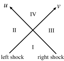
Figure 1: Schematic picture of the spacetime of colliding high-energy particles.

The high-energy two-particle system in four dimensions has been discussed to some extent before the appearance of the brane world scenarios. The metric of one high-energy particle was obtained by Aichelburg and Sexl AS71 by boosting the Schwarzschild black hole to the speed of light with fixed energy $\mu$. The gravitational wave emission in the axisymmetric system of two combined Aichelburg-Sexl particles was studied by D’Eath D'Eath and D’Eath and Payne DP92 (summarized in D96 ). A schematic picture of the spacetime with two Aichelburg-Sexl particles is shown in Fig. 1. Two particles collide at the speed of light. The gravitational field of each incoming particle is infinitely Lorentz-contracted and forms a shock wave. Except at the shock waves, the spacetime is flat before the collision (i.e., regions I, II, and III). After the collision, the two shocks nonlinearly interact with each other, and the spacetime within the future lightcone of the collision (i.e., region IV) becomes highly curved. The ultimate goal would be to clarify the structure of region IV. If this is possible, the black hole production cross section and the gravitational waves emitted in the relaxation process could be determined. But this analysis is difficult because of the quite complicated structure of the gravitational field, and no one has succeeded in deriving the metric in region IV even numerically.

Nonetheless, one can estimate the lower bound on the black hole production cross section only with the knowledge of regions I, II, and III. This can be done by finding an apparent horizon (AH), because the AH existence is a sufficient condition for the event horizon (EH) formation W84 (assuming the cosmic censorship P69 ). As mentioned in D'Eath ; DP92 ; D96 (see also EG02 ), Penrose (1974, unpublished) constructed an AH on the slice $u=0,v<0$ and $v=0,u<0$ in the head-on collision case in four-dimensional spacetime. Because this AH has intrinsic geometry of combined two flat disks, it is often called the Penrose flat disks. Eardley and Giddings EG02 extended the AH solution of Penrose flat disks to positive impact parameters. They analytically derived the maximal impact parameter $\hat{b}_{max}$ for the AH formation in a grazing collision in the four-dimensional spacetime. Subsequently, one of us and Nambu YN03 extended this analysis to higher-dimensional spacetimes. The values of $\hat{b}_{max}$ in $D$-dimensional cases were obtained numerically, and they can be well approximated by $\hat{b}_{max}\simeq 1.5\times 2^{-1/(D-3)}r_{h}(2\mu)$.

The AH method provides a lower bound on the true collision cross section. This lower bound depends on the slice used to determine the AH and becomes larger if a future slice is chosen. Indeed, the maximal impact parameter of the AH formation will be larger for such a slice (simply because it is possible that, for a given impact parameter, an AH has not yet formed on the old slice, while it forms by the time a later slice is reached). The lower bound would asymptotically approach the exact cross section as we move into the far future. Because of the monotonic growth, the further we move into the future, the smaller the difference between the true cross section and the estimate provided by the AH method would become.

After the works of EG02 ; YN03 , one of us raised doubts in the validity of the setup of the high-energy two-particle system R04 , because of possible strong curvature effects in colliding shocks. However, this problem was later shown to be an artifact of the unphysical classical point-particle limit: for a particle described by a small quantum wavepacket large curvatures do not arise GR04 (see also R04-2 ). Roughly, if a wave packet of Planck size $\delta z$ is taken, curvature remains sufficiently small, while corrections to the Aichelburg-Sexl geometry are $O(\delta z/r_{h})\ll 1$. This argument justified the use of the Aichelburg-Sexl two-particle system to compute the black hole production cross section in elementary particle collisions. See also Y05 , R04-3 for other characteristics of incoming particles that could affect black hole formation.

In light of the above discussion, the purpose of this paper is as follows. In the previous analysis EG02 ; YN03 , the AH was constructed on the union of the two incoming shocks $u=0,v<0$ and $v=0,u<0$ (referred below as the old slice). However, it is clear from Fig. 1 that this slice is not at all optimal in the sense that there exist other slices within regions I, II, III, located to the future of the old slice. Motivated by this observation, we proceed with the AH analysis on the slice of the future light cone of the shock collision plane, given by the union of the outgoing shocks $u=0,v>0$ and $v=0,u>0$ (referred below as the new slice). This slice is optimal in the sense that it is the future-most slice that can be taken without the knowledge of region IV. By this analysis, we will improve the lower bound on the cross section of the black hole production. In addition, using the area theorem H71 , we will find restrictions on the mass $M$ and the angular momentum $J$ of the final state (i.e. the produced black hole after the balding phase). This part of the analysis is new compared to YN03 , and provides indirect information about the spacetime structure of region IV of the Aichelburg-Sexl two-particle system.

This paper is organized as follows. In the next section, we explain the system setup and derive the AH equation and the boundary conditions in the new slice. Then we present the analytic solution of the AH equation in the head-on collision case and explain the numerical method for the more physically important grazing collision case. In Sec. III, we present our numerical results. We summarize the results for the maximal impact parameter and discuss the mass $M$ and angular momentum $J$ of the final state, as allowed by the area theorem. Sec. IV is devoted to the summary and discussion.

Our new lower bounds on $\sigma_{\rm BH}$, most precise to date, are summarized in Table II.

II Apparent horizons in the high-energy particle system

II.1 System setup

We begin by reviewing the Aichelburg-Sexl metric, describing the gravitational field of a high-energy particle. Following the analysis in EG02 ; YN03 , we use the metric of a massless point particle of AS71 ; D'Eath ; DH ; EG02 that is obtained by boosting the Schwarzschild black hole to the speed of light with fixed energy $\mu=\gamma M$. The result is

$$ds^{2}=-d\bar{u}d\bar{v}+d\bar{r}^{2}+\bar{r}^{2}d\bar{\Omega}_{D-3}^{2}+\Phi(\bar{r})\delta(\bar{u})d\bar{u}^{2},$$ (3)

$$\Phi(\bar{r})=\left\{\begin{array}[]{ll}-2\log\bar{r}&(D=4),\\ {2}/{(D-4)\bar{r}^{D-4}}&(D\geq 5).\end{array}\right.$$ (4)

Here we adopt $r_{0}=\left(8\pi G_{D}\mu/\Omega_{D-3}\right)^{1/(D-3)}$ as the unit of length, which is close to $r_{h}(2\mu)$. The delta function in Eq. (3) indicates that the coordinate system is discontinuous at $\bar{u}=0$, and that a distributional Riemann curvature (i.e., a gravitational shock wave) is located there. The continuous coordinates are introduced by

$$\bar{u} =u,$$ (5)

$$\bar{v} =\left\{\begin{array}[]{ll}v-2\log r\theta(u)+{u\theta(u)}/{r^{2}}&(D=4),\\ v+{2\theta(u)}/{(D-4)r^{D-4}}+{u\theta(u)}/{r^{2D-6}}&(D\geq 5),\end{array}\right.$$ (8)

$$\bar{r} =r\left(1-\frac{u}{r^{D-2}}\theta(u)\right),$$ (9)

$$\bar{\phi}_{i} =\phi_{i},$$ (10)

where $\bar{\phi}_{i}$ are the coordinates on the $(D-3)$-sphere. The metric becomes D'Eath ; R04

$$ds^{2}=-dudv+\left[1+(D-3)\frac{u}{r^{D-2}}\theta(u)\right]^{2}dr^{2}+r^{2}\left[1-\frac{u}{r^{D-2}}\theta(u)\right]^{2}d\Omega^{2}_{D-3},$$ (11)

where $\theta(u)$ denotes the Heaviside step function. Note that $u=r^{D-2}$ is a coordinate singularity for $u\geq 0$, because the $(D-3)$-sphere shrinks to zero size. Thus the $\bar{u}>0$ region is mapped onto the $0<u\leq r^{D-2}$ region by this coordinate transformation.

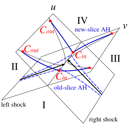
Figure 2: Schematic picture of the spacetime of colliding high-energy particles with $(D-3)$ dimensions suppressed. The schematic shape of AH on the new slice ($u>0,v=0$ and $v>0,u=0$) is shown by solid lines, while the AH on the old slice ($u<0,v=0$ and $v<0,u=0$) is shown by dashed lines. Dotted lines indicate coordinate singularities.

By causality, we can construct the metric of a high-energy two-particle system in regions I, II, and III by simply combining the metric of the left and the right particles, because there is no interaction before the collision. Figure 2 shows the schematic spacetime structure adding one dimension to Fig. 1. Our goal is to construct an AH on the new slice, i.e., on the union of the two null surfaces $u=0,~{}v>0$ and $u>0,~{}v=0$. By the left-right symmetry (we work in the center-of-mass frame), it is sufficient to consider the $u>0,~{}v=0$ surface. We introduce a coordinate $\phi$ such that the metric in region II is given by

$$ds^{2}=-dudv+\left[1+(D-3)\frac{u}{r^{D-2}}\right]^{2}dr^{2}+r^{2}\left[1-\frac{u}{r^{D-2}}\right]^{2}\left(d\phi^{2}+\sin^{2}\phi d\Omega^{2}_{D-4}\right).$$ (12)

The radial coordinate $r$ in region II is adapted to the left particle, which is thus located at $r=0$. In these coordinates, the right particle will cross the transverse collision plane $u=v=0$ at a point distance $b$ from the origin, where $b$ is the impact parameter. We will choose coordinate $\phi$ so that this point is $r=b$, $\phi=0$. This setup is identical to the one used in EG02 and YN03 .

II.2 AH equation and boundary conditions

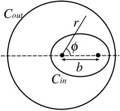
Figure 3: Schematic picture of the boundaries $C_{in}$ and $C_{out}$. We should solve for $h(r,\phi)$ in the region surrounded by the two boundaries.

The schematic shape of the AH on the new slice is also shown in Fig. 2. Because $u=r^{D-2}$ is a coordinate singularity, we have two boundaries in this analysis: $C_{in}$ at $u=v=0$ and $C_{out}$ at $u=r^{D-2},v=0$. We show the schematic shapes of $C_{in}$ and $C_{out}$ in Fig. 3. Between these boundaries, the AH shape is specified by an unknown function $u=h(r,\phi)$. The tangent vector $k^{\mu}$ of the null geodesic congruence of the AH surface can be found in terms of this function using metric (12) and is given by

$$k^{u} =\frac{1}{2}\left\{\left[1+(D-3)\frac{h}{r^{D-2}}\right]^{-2}h_{,r}^{2}+r^{-2}\left(1-\frac{h}{r^{D-2}}\right)^{-2}h_{,\phi}^{2}\right\},$$ (13)

$$k^{v} =2,$$ (14)

$$k^{r} =\left[1+(D-3)\frac{h}{r^{D-2}}\right]^{-2}h_{,r},$$ (15)

$$k^{\phi} =r^{-2}\left(1-\frac{h}{r^{D-2}}\right)^{-2}h_{,\phi}.$$ (16)

Imposing that this congruence has zero expansion, we get the AH equation:

$$\left(r^{D-2}-h\right)^{2}\left\{h_{,rr}+(D-3)\frac{h_{,r}}{r}\left[1+\frac{(D-2)h-(3/2)rh_{,r}}{r^{D-2}+(D-3)h}+\frac{(D-2)h-(1/2)rh_{,r}}{r^{D-2}-h}\right]\right\}+\\ r^{-2}\left[r^{D-2}+(D-3)h\right]^{2}\left\{h_{,\phi\phi}+(D-4)\cot\phi h_{,\phi}+\frac{h_{,\phi}^{2}}{2}\left[\frac{D-3}{r^{D-2}+(D-3)h}-\frac{D-7}{r^{D-2}-h}\right]\right\}\\ =0.$$ (17)

Now we consider the boundary conditions. At $C_{in}$, the continuity of the AH requires

$$h(r,\phi)=0.$$ (18)

Another condition comes from the continuity of the null tangent vector (up to a factor). This condition is equivalent to $k^{u}(x)k^{v}(x^{\star})=k^{v}(x)k^{u}(x^{\star})$ or

$$\left(h_{,r}^{2}+r^{-2}h_{,\phi}^{2}\right)\big{|}_{x}\left(h_{,r}^{2}+r^{-2}h_{,\phi}^{2}\right)\big{|}_{x^{\star}}=16,$$ (19)

where $x^{\star}$ denotes the point symmetric to $x$ with respect to the center of $C_{in}$ (i.e. the point $r=b/2,\phi=0$).

Now we turn to the boundary conditions at $C_{out}$. Because $u=r^{D-2}$ is a coordinate singularity, $C_{out}$ has to be located at some fixed unknown radius $r=r_{max}$ so that the AH is continuous. Hence we have

$$h=r_{max}^{D-2},$$ (20)

on $C_{out}$.

The last boundary condition follows by imposing the continuity of $k^{\mu}$ on $C_{out}$. For this purpose, we should translate $k^{\mu}$ into the $(\bar{u},\bar{v},\bar{r},\bar{\phi})$ coordinates. Using the fact that $h$ behaves like

$$h=r_{max}^{D-2}+h_{,r}(\phi)(r-r_{max})+\frac{1}{2}h_{,rr}(\phi)(r-r_{max})^{2}+\cdots$$ (21)

in the neighborhood of $C_{out}$, we obtain

$$k^{\bar{u}} =1,$$ (22)

$$k^{\bar{v}} =r_{max}^{6-2D}-\frac{4}{(D-2)r_{max}^{D-3}}\left[h_{,r}-(D-2)r_{max}^{D-3}\right]/F,$$ (23)

$$k^{\bar{r}} =-r_{max}^{3-D}+2(D-2)^{-1}h_{,r}/F,$$ (24)

$$k^{\bar{\phi}} =2r_{max}^{2D-6}\left[h_{,r}-(D-2)r_{max}^{D-3}\right]^{-2}(r-r_{max})^{-1}h_{,r\phi}/F.$$ (25)

where

$$F=(D-2)^{-2}h_{,r}^{2}+r_{max}^{2D-6}\left[h_{,r}-(D-2)r_{max}^{D-3}\right]^{-2}h_{,r\phi}^{2}.$$ (26)

In order that $k^{\mu}$ be continuous, $k^{\bar{v}}$ should be constant for all $\phi$:

$$\left[{h_{,r}-(D-2)r_{max}^{D-3}}\right]/F=\bar{B}.$$ (27)

There are also two other conditions given by

$$k^{\bar{r}}=Br_{max}^{3-D}\cos\phi,$$ (28)

$$k^{\bar{\phi}}=-\frac{Br_{max}^{3-D}}{\bar{r}}\sin\phi,$$ (29)

where we have used the symmetry of this system. (These conditions are analogous to the conditions for smoothness of a non-axisymmetric surface written in cylindrical coordinates.) Here, $B$ and $\bar{B}$ are related as

$$\bar{B}=\frac{(D-2)r_{max}^{3-D}}{4}(1-B^{2})$$ (30)

by the null condition $k_{\mu}k^{\mu}=0$. Using Eqs. (24), (27), (28) and (30), we derive

$$h_{,r}=(D-2)r_{max}^{D-3}\left(1+\frac{1-B^{2}}{1+B^{2}+2B\cos\phi}\right).$$ (31)

This is the second boundary condition at $C_{out}$. Although we have not used Eqs. (25) and (29), we can easily check the consistency. The boundary condition (31) is also consistent with the AH equation (17). Substituting the series (21) into Eq. (17), the leading-order term is

$$h_{,r\phi\phi}+(D-4)\cot\phi h_{,r\phi}+\frac{(1/2)(D-7)h_{,r\phi}^{2}}{h_{,r}-(D-2)r_{max}^{D-3}}\\ +\frac{(D-3)}{2(D-2)^{2}}r_{max}^{6-2D}h_{,r}\left[h_{,r}-(D-2)r_{max}^{D-3}\right]\left[h_{,r}-2(D-2)r_{max}^{D-3}\right]=0.$$ (32)

By substituting Eq. (31) into the left-hand side, we can confirm that this equation is actually satisfied.

In summary, there are two boundary conditions for each boundary: Eqs. (18) and (19) for $C_{in}$ and Eqs. (20) and (31) for $C_{out}$. We should determine the shape of the boundary $C_{in}$ and the values of $r_{max}$ and $B$, as well as the function $h(r,\phi)$, so as to be consistent with these four boundary conditions.

The AH equation (17) is highly nonlinear and finding analytic solutions for $b\neq 0$ seems almost impossible even for $D=4$. This is in contrast with the old-slice case EG02 , where the AH equation was given by the Laplace equation. But as a numerical problem, the new case is quite similar to the old case except that one boundary is added (the $C_{in}$ boundary conditions are the same as in the old case). We can solve this problem by extending the numerical techniques developed in YN03 as explained later.

II.3 Head-on collision case

In the head-on collision case, we can solve the AH equation analytically. In this case, the function $h$ depends only on $r$ and the boundaries $C_{in}$ and $C_{out}$ are given by $r=r_{min}$ and $r=r_{max}$, respectively. The equation and the boundary conditions become

$$h_{,rr}+\frac{(D-3)}{r}h_{,r}\left[1+\frac{(D-2)h-(3/2)rh_{,r}}{r^{D-2}+(D-3)h}+\frac{(D-2)h-(1/2)rh_{,r}}{r^{D-2}-h}\right]=0,$$ (33)

$$h(r_{min})=0,$$ (34)

$$h_{,r}(r_{min})=2,$$ (35)

$$h(r_{max})=r_{max}^{D-2},$$ (36)

$$h_{,r}(r_{max})=2(D-2)r_{max}^{D-3}.$$ (37)

In $D=4$ case, the solution is given by

$$h=2r^{2}\log r,$$ (38)

$$r_{min}=1,$$ (39)

$$r_{max}=\sqrt{e}.$$ (40)

In $D\geq 5$ cases, the solutions are as follows:

$$h=\frac{2}{(D-4)}r^{D-2}\left(r^{D-4}-1\right),$$ (41)

$$r_{min}=1,$$ (42)

$$r_{max}=\left(\frac{D-2}{2}\right)^{1/(D-4)}.$$ (43)

The total AH area is easily calculated. Restoring the length units, we have

$$A_{D-2}=\frac{2\Omega_{D-3}}{(D-2)}\left(\frac{8\pi G_{D}\mu}{\Omega_{D-3}}\right)^{(D-2)/(D-3)}.$$ (44)

This is exactly the same value as the area of two Penrose flat disks (i.e., the AH on the old slice) given in EG02 . This coincidence can be interpreted as follows. Because the null geodesic congruence of the Penrose flat disk does not have shear, the expansion rate does not change (i.e. stays equals to zero) while propagating into region II according to Raychaudhuri’s equation. Hence, the null geodesic congruence of the AH on the new slice $v=0,u>0$ is the same as that of the Penrose flat disk, and the areas of the two AHs coincide.

However, for positive impact parameters (grazing collisions), the shear of the null geodesic congruence of the AH on the old slice will be non-zero. While propagating, the expansion rate becomes negative according to Raychaudhuri’s equation, and the null geodesic congruence of the AH on the new slice will not be the same as on the old slice. This suggests that, using the new slice, we should find larger AH areas and larger maximal impact parameters compared to those in the previous results of EG02 ; YN03 .

II.4 Numerical method for grazing collision

In the grazing collision case, a numerical calculation is required to determine the AH. To solve the AH equation, we introduce coordinates $(\tilde{r},\tilde{\phi})$ by

$$r\cos\phi =\tilde{r}\cos\tilde{\phi}+b/2,$$ (45)

$$r\sin\phi =\tilde{r}\sin\tilde{\phi}.$$ (46)

In these coordinates, the central point of $C_{in}$ is given by $\tilde{r}=0$. (Because of the left-right symmetry, $C_{in}$ will be symmetric with respect to the lines $\tilde{\phi}=0$ and $\tilde{\phi}=\pi/2$.) We specify the boundaries $C_{in}$ and $C_{out}$ by

$$\tilde{r} =g_{in}(\tilde{\phi}),$$ (47)

$$\tilde{r} =g_{out}(\tilde{\phi})=-(1/2)b\cos\phi+\left[r_{max}^{2}-(1/4)b^{2}\sin^{2}\tilde{\phi}\right]^{1/2},$$ (48)

respectively. We make a further transformation

$$R=\frac{\tilde{r}-g_{in}(\tilde{\phi})}{g_{out}(\tilde{\phi})-g_{in}(\tilde{\phi})},$$ (49)

and solve the AH equation using the $(R,\tilde{\phi})$ coordinates. The advantage of these coordinates is that $C_{in}$ and $C_{out}$ are specified by $R=0$ and $R=1$, respectively, and the boundary conditions are easily imposed.

The following algorithm was used in the numerical solution of our boundary value problem. First, some test boundaries $C_{in}$ and $C_{out}$ are taken, and the solution of the AH equation satisfying only the two boundary conditions (18) and (20) is constructed (using a finite-difference discretization of the partial differential equation, and a convergent iterative procedure). Next, the difference from the boundary condition (19) is calculated:

$$\Delta_{in}(\tilde{\phi})=\left(h_{,r}^{2}+r^{-2}h_{,\phi}^{2}\right)\big{|}_{x}\left(h_{,r}^{2}+r^{-2}h_{,\phi}^{2}\right)\big{|}_{x^{\star}}-16,$$ (50)

and $C_{in}$ is modified as follows:

$$g_{in}^{\rm next}(\tilde{\phi})=g_{in}(\tilde{\phi})+\epsilon_{in}\Delta_{in}(\tilde{\phi}).$$ (51)

The $C_{out}$ is also modified at this step, as follows. Recall that $C_{out}$ is characterized by $r_{max}$ and $B$. We determine $B$ using Eq. (31) at $\tilde{\phi}=0$ and calculate the difference from the boundary condition (31) at $\tilde{\phi}=\pi$:

$$\Delta_{out}=h_{,r}-2(D-2)r_{max}^{D-3}/{(1-B)}.$$ (52)

Using this value, we modify $r_{max}$ as follows:

$$r_{max}^{\rm next}=r_{max}+\epsilon_{out}\Delta_{out}.$$ (53)

If we choose $\epsilon_{in}$ and $\epsilon_{out}$ appropriately, we can make the boundaries converge by iterating these steps. We truncated the iteration when the absolute values of $\Delta_{in}(\tilde{\phi})$ and $\Delta_{out}$ become less than $10^{-5}$.

Table 1: The error estimated by the difference from the $C_{out}$ boundary condition, i.e., Eq. (54) evaluated at $b=b_{max}$. The error decreases by a factor of about $4$ when doubling the resolution. This indicates the correctness of our numerical calculations.

$D$	$4$	$5$	$6$	$7$	$8$	$9$	$10$	$11$
$(25\times 50)$ grids	$0.21\%$	$2.0\%$	$4.2\%$	$-$	$-$	$-$	$-$	$-$
$(50\times 100)$ grids	$0.052\%$	$0.49\%$	$1.1\%$	$1.9\%$	$3.0\%$	$4.0\%$	$4.6\%$	$5.1\%$
$(100\times 200)$ grids	$-$	$-$	$0.29\%$	$0.50\%$	$0.75\%$	$1.1\%$	$1.4\%$	$1.8\%$

To evaluate the numerical error, the following method was used. In the numerical method explained above, we could use only two grid points to impose the boundary condition at $C_{out}$, because the values to be determined are only $r_{max}$ and $B$. In principle, the boundary conditions (31) should be satisfied at the remaining grid points because Eq. (31) is compatible with the AH equation in the neighborhood of $C_{out}$, as expressed by (32). However, in practice, because of the finiteness of the number of grid points, small differences from the boundary condition (31) will be present in the intermediate grid points ($0<\phi<\pi$). This suggests to estimate the characteristic error as follows:

$$\delta=\frac{1}{N}\sum\left|1-h_{,r}^{-1}(D-2)r_{max}^{D-3}\left(1+\frac{1-B^{2}}{1+B^{2}+2B\cos\phi}\right)\right|,$$ (54)

where the sum is taken over all grid points on $C_{out}$, and $N$ is the total number of these points.

Table I summarizes the resolution of the grids used to discretize the $(R,\tilde{\phi})$ coordinates in our computations, as well as the error $\delta$ at $b=b_{max}$. We observed that the error estimated by $\delta$ becomes larger as $b$ increases, and takes the largest value at $b=b_{max}$; it also becomes larger for larger $D$. For fixed $b$ and $D$, the $\delta$ typically decreases by a factor of about $4$ if a grid with double resolution (i.e. with 4 times as many points) is used. Such behavior of the error strongly indicates the correctness of our numerical program, and the convergence to the continuum limit. Although $\delta$ seems somewhat large for large $D$, it turned out that the error in $b_{max}$ is much smaller, as follows by comparing the values of $b_{max}$ obtained for different grid resolutions. We estimate the error in $b_{max}$ at the level of about $0.2\%$ for all $D$. Instead, the $\delta$ reflects the error in the AH shape. To summarize, the error in Figs. 4-8, 10-14 is roughly of the magnitude given in Table I, while the error in Table II is about 0.2%.

III Numerical results

In this section, we present the numerical results for the AHs in the grazing collision. The section is divided into two parts. We first provide the results for the AH shape and the maximal impact parameter of the AH formation. Next, we introduce two quantities that indicate the amount of energy trapped by the AH and discuss the final state of the produced black hole, as allowed or prohibited by the area theorem.

III.1 AH shape and the maximal impact parameter

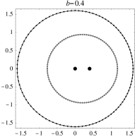
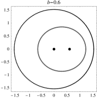
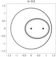
Figure 4: The shape of $C_{in}$ and $C_{out}$ for $b/r_{0}=0.4,0.6,0.8,0.841$ in the $D=4$ case. Two dots in each figure indicate the location of incoming particles. The old-slice AHs in EG02 for $b/r_{0}=0.4,0.6,0.8$ are shown by gray lines. We could not find the AH for $b/r_{0}=0.842$.

Figure 4 shows the shapes of $C_{in}$ and $C_{out}$ for various values of $b$ in the $D=4$ case. The old-slice AHs of Eardley and Giddings EG02 are also shown. As $b$ increases, $C_{in}$ becomes oblate, and $r_{max}$ becomes smaller. For small $b$, $C_{in}$ and the corresponding boundary curve of the old-slice AH almost coincide, which again indicates the correctness of our numerical program. For larger $b$, $C_{in}$ lies outside the old-slice AH curve. For even larger $b$, we have a situation when there exists an AH in the new slice, while there is no AH in the old slice. The $b_{max}$ becomes about 5% larger than the previous result of EG02 .

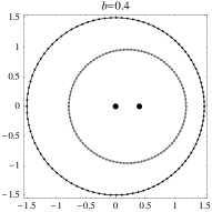
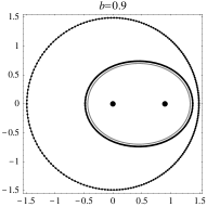
Figure 5: The shapes of $C_{in}$ and $C_{out}$ for $b=0.4,0.9,1.1,1.145$ in the $D=5$ case. Two dots in each figure indicate the location of the incoming particles. The old-slice AHs of YN03 for $b/r_{0}=0.4,0.9$ are shown by gray lines. We could not find the AH for $b/r_{0}=1.146$.

Figure 5 shows the shapes of $C_{in}$ and $C_{out}$ in the $D=5$ case. In this case, $r_{max}$ is almost constant for all $b$ and the shape of $C_{in}$ becomes oblate as $b$ increases. It is quite interesting that $C_{in}$ becomes non-convex around $b=b_{max}$. The value of $b_{max}$ is about 18% larger than the previous result of Yoshino and Nambu YN03 , which leads to 40% larger cross section of the AH formation, the present value being $\sigma_{\rm AH}\simeq 1.5\pi\left[r_{h}(2\mu)\right]^{2}$.

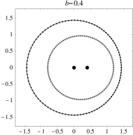
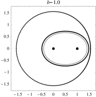
Figure 6: The shape of $C_{in}$ and $C_{out}$ for $b/r_{0}=0.4,1.0,1.3,1.333$ in the $D=6$ case. Two dots in each figure indicate the location of the incoming particles. The old-slice AHs of YN03 for $b=0.4,1.0$ are shown by gray lines. We could not find the AH for $b/r_{0}=1.334$.

Figure 6 shows the shapes of $C_{in}$ and $C_{out}$ in the $D=6$ case. In this case, $r_{max}$ becomes larger as $b$ increases. The shape of $C_{in}$ at $b=b_{max}$ is even more non-convex than that in the $D=5$ case. The value of $b_{max}$ is about 26% larger than the previous result of YN03 . This leads to 59% larger cross section of the AH formation, the present value being $\sigma_{\rm AH}\simeq 2.1\pi\left[r_{h}(2\mu)\right]^{2}$.

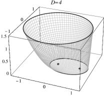
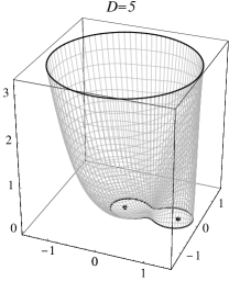
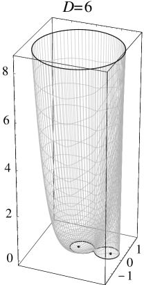
Figure 7: Three-dimensional plots of the AH shape function at $b=b_{max}$ for $D=4,5,$ and $6$. The AH becomes taller for larger $D$ as a consequence of the growing power exponent in the boundary condition (20).

In Fig. 7, we plot the AH shape function $h(r,\phi)$ at $b=b_{max}$ for $D=4,5,$ and $6$. The AH becomes taller for larger $D$ as a consequence of the growing power exponent in the boundary condition (20).

For $D\geq 7$, the shapes of $C_{in}$ and $C_{out}$ and the horizon shape behave qualitatively similarly to the $D=6$ case, and we do not present them here in detail.

Figure 8: The relation between $b/r_{0}$ and $r_{min}/r_{0}$, where $r_{min}=g_{in}(\pi/2)$. The maximal impact parameter occurs at $dr_{min}/db=-\infty$.

Table 2: The value of $b_{max}/r_{0}$, the ratio of the increase in the maximal impact parameter, and the value of the AH formation cross section $\sigma_{\rm AH}$ (which provides a rigorous lower bound for $\sigma_{\rm BH}$).

$D$	$4$	$5$	$6$	$7$	$8$	$9$	$10$	$11$
$b_{max}/r_{0}$	$0.841$	$1.145$	$1.333$	$1.441$	$1.515$	$1.570$	$1.613$	$1.648$
$b_{max}/\hat{b}_{max}-1$	$5\%$	$18\%$	$26\%$	$29\%$	$29\%$	$30\%$	$30\%$	$30\%$
$\sigma_{\rm AH}/\pi\left[r_{h}(2\mu)\right]^{2}$	$0.71$	$1.54$	$2.15$	$2.52$	$2.77$	$2.95$	$3.09$	$3.20$

Figure 9: Summary of the $b_{max}/r_{h}(2\mu)$ values ($\circ$) and the previous $\hat{b}_{max}/r_{h}(2\mu)$ values ($\times$) for $D=4,...,11$.

Figure 8 shows the minimum radius of $C_{in}$, $r_{min}\equiv g_{in}(\pi/2)$, as a function of $b$ for $D=4,...,11$. The maximal impact parameter occurs at $dr_{min}/db=-\infty$. From this figure, we can read off the values of $b_{max}$.

Table II summarizes the numerical results for $b_{max}$, which are the most important output of our analysis. For $5\leq D\leq 11$, the values of $b_{max}$ increase by $18$-$30$% compared to the previous values of $\hat{b}_{max}$ in YN03 . Correspondingly, the values of the cross section of the AH formation $\sigma_{\rm AH}/\pi\left[r_{h}(2\mu)\right]^{2}$ increase by $40$-$70$ %. This indicates that the black hole production rate in accelerators can be quite a bit larger compared to the previous estimates, this tendency being especially enhanced for larger $D$. In the $D=4$ case, which may have only astrophysical applications, we find only a modest 5% improvement in $b_{max}$ compared to EG02 . We compare the present values of $b_{max}/r_{h}(2\mu)$ with the previous values of $\hat{b}_{max}/r_{h}(2\mu)$ in Figure 9.

III.2 Trapped energy and final state of the produced black hole

Assuming the cosmic censorship P69 , an event horizon (EH) must be present outside the found AHs (see W84 for a proof). Moreover, the area theorem H71 states that the EH area never decreases. Hence one naturally expects that the AH mass defined by

$$M_{\rm AH}=\frac{(D-2)\Omega_{D-2}}{16\pi G_{D}}\left(\frac{A_{D-2}}{\Omega_{D-2}}\right)^{(D-3)/(D-2)}$$ (55)

provides the lower bound of the irreducible mass $M_{irr}$ of the final Kerr black hole. We should mention that for this statement to be rigorously justified, the area of an arbitrary surface outside of the AH in a given slice should be larger than that of the AH. In the old slice analyzed in EG02 ; YN03 this property actually holds. On the other hand, on the new slice analyzed here we can find a counterexample. In the head-on collision case, for example, the union of two surfaces $r=r_{c}>r_{max},0\leq u\leq r_{c}^{D-2},v=0$ and $r=r_{c},0\leq v\leq r_{c}^{D-2},u=0$ is closed, lies outside of the AH, and has zero area. Thus there is no rigorous reason why in the present analysis $M_{\rm AH}$ should provide the lower bound on the final mass.

Nevertheless, we can still find a rigorous lower bound on $M_{irr}$, arguing as follows. The intersection of the AH and $u=v=0$ is given by $C_{in}$. Let us denote the intersection of the EH and $u=v=0$ by $C_{\rm EH}$. This curve must lie outside $C_{in}$. Further, one can show that the area $A_{\rm EH}$ of the intersection of the EH with the old slice is equal to twice the area of the region surrounded by $C_{\rm EH}$ calculated with the $(D-2)$-dimensional flat metric. It follows that $A_{\rm EH}$ is bounded below by $A_{lb}$, the latter quantity being defined as twice the area of the region surrounded by $C_{in}$, calculated with the same flat metric. Hence the rigorous lower bound on $M_{irr}$ is given by

$$M_{lb}=\frac{(D-2)\Omega_{D-2}}{16\pi G_{D}}\left(\frac{A_{lb}}{\Omega_{D-2}}\right)^{(D-3)/(D-2)}.$$ (56)

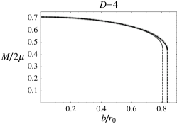
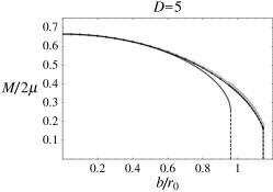
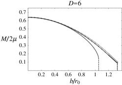
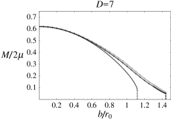
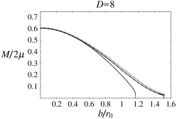
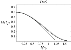
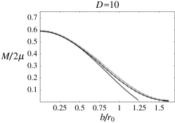
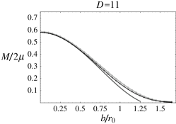
Figure 10: The rigorous lower bound $M_{lb}$ of the final irreducible mass (black lines) and the indicator of the trapped energy $M_{\rm AH}$ (light gray lines) for $D=4,...,11$. The previous value of the AH mass $\hat{M}_{\rm AH}$ of EG02 ; YN03 are also shown by dark gray lines.

This $M_{lb}$ as a function of $b$ is shown in Fig. 10. The non-rigorous bound $M_{\rm AH}$ is also included, because under some additional assumptions it may still provide the energy trapped by the produced black hole. For example, the Hawking quasi-local mass H68 calculated on the AH coincides with $M_{\rm AH}$. The old-slice value of the AH mass $\hat{M}_{\rm AH}$ as found in EG02 ; YN03 is also shown. We see that $M_{lb}$ and $M_{\rm AH}$ take close values, $M_{\rm AH}$ being slightly larger. Although $M_{lb}$ and $M_{\rm AH}$ are close to $\hat{M}_{\rm AH}$ for small $b$, they becomes significantly larger around $b=\hat{b}_{max}$, especially in the higher-dimensional cases.

Now we consider the mass $M$ and the angular momentum $J$ of the final Kerr black hole which are allowed by the area theorem:

$$M_{irr}\geq M_{lb}.$$ (57)

Here $M_{irr}=M_{irr}(M,J)$ is the irreducible mass of the Kerr black hole, which is defined, just as in four dimensions, as the mass of a Schwarzschild black hole having the same horizon area. It is thus related to the Kerr black hole horizon area $A_{Kerr}$ by the formula:

$$A_{Kerr}=\Omega_{D-3}r_{h}^{D-3}(M_{irr}).$$

The left-hand side of this equation can be easily computed using the explicit $D$-dimensional Kerr black hole metric MP86 , which gives the relation

$$r_{h}^{D-2}(M_{irr})=r_{h}^{D-3}(M)r_{k}(M,J).$$ (58)

Here $r_{k}(M,J)$ is the Kerr black hole horizon radius which satisfies the following equation MP86 :

$$r_{k}^{2}(M,J)+\left[\frac{(D-2)J}{2M}\right]^{2}=r_{h}^{D-3}(M)r_{k}^{5-D}(M,J).$$ (59)

The total energy and the angular momentum of the system before the collision are $2\mu$ and $b\mu$, respectively. Denoting

$$\xi =M/2\mu,$$ (60)

$$\zeta =J/b\mu,$$ (61)

the final state of the produced black hole will be specified by a point in $(\xi,\zeta)$-plane with $0\leq\xi\leq 1$ and $0\leq\zeta\leq 1$.

For $D=4,5$ there exists an upper limit on the black hole angular momentum for a fixed mass MP86 :

$$J\leq J_{\star}(M)\equiv\left\{\begin{array}[]{ll}(1/2)Mr_{h}(M)&(D=4),\\ (2/3)Mr_{h}(M)&(D=5),\end{array}\right.$$ (62)

Region (i) consisting of points satisfying the opposite condition $J>J_{\star}(M)$ should be a priori excluded from the $(\xi,\zeta)$-diagram.

According to the above discussion, region (ii) corresponding to black holes violating the area theorem (57) can also be excluded. The remaining points constitute the allowed region (iii).

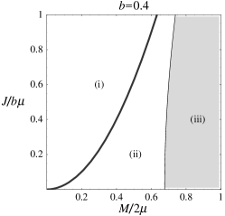
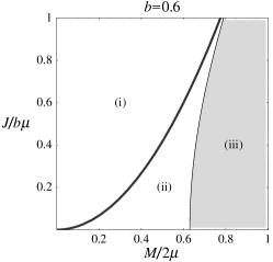
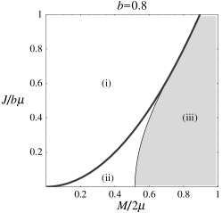
Figure 11: The regions (i), (ii) and (iii) in the $(\xi,\zeta)$-plane for $b=0.4,0.6,0.8$ in the $D=4$ case.

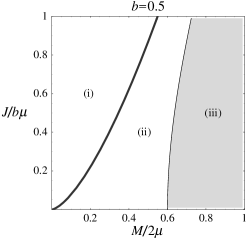
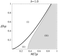
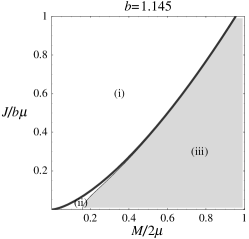
Figure 12: The regions (i), (ii) and (iii) in the $(\xi,\zeta)$-plane for $b=0.5,1.0,1.145$ in the $D=5$ case.

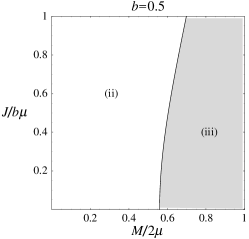
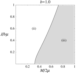
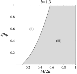
Figure 13: The regions (ii) and (iii) in the $(\xi,\zeta)$-plane for $b=0.5,1.0,1.3$ in the $D=6$ case.

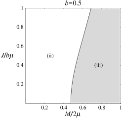
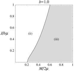
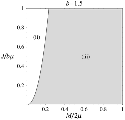
Figure 14: The regions (ii) and (iii) in the $(\xi,\zeta)$-plane for $b=0.5,1.0,1.5$ in the $D=9$ case.

Figures 11-14 show regions (i), (ii), (iii) for $D=4,5,6,$ and $9$ for some selected values of $b$. We see that the condition $M_{irr}>M_{lb}$ gives a stronger restriction on the final state $(\xi,\zeta)$ than the simple condition $M>M_{lb}$. This difference becomes quite noticeable especially for $b\simeq b_{max}$ in the $D=4$ and $5$ cases. This result indicates that $M$ should be quite a bit larger than $M_{lb}$ at $b\simeq b_{max}$, because almost 100% angular momentum should be radiated away if $M\simeq M_{lb}$, which would be quite unnatural.

Unfortunately, we cannot find a non-trivial upper bound for the angular momentum $J$ of the final Kerr black hole. (If the boundary of region (iii) intersected the $\xi=1$ line at $\zeta<1$, we would be able to find such a bound.) On the other hand, it is interesting to note that our results are quite consistent with previous numerical simulations of gravitational collapse of rapidly rotating bodies in four dimensions (see SS04 and references therein). In these works, the authors found a necessary condition for black hole formation expressed as

$$q\equiv J_{\rm system}/J_{\star}(M_{\rm system})\lesssim 1,$$ (63)

where $M_{\rm system}$ and $J_{\rm system}$ are the total gravitational mass and angular momentum of the system. In our system, the value of $q$ at $b=b_{max}$ is

$$q=\left\{\begin{array}[]{ll}0.84&(D=4),\\ 0.93&(D=5),\end{array}\right.$$ (64)

which is in agreement with (63). It should be pointed out that for the five-dimensional black ring solutions ER02 there is no upper bound on $q$, and thus we expect that criterion (63) in the five-dimensional case holds only for formation of the AH with spherical topology.

IV Summary and discussion

In this paper, we have analyzed the AH formation in the high-energy particle collision using a new slice $u=0,v>0$ and $v=0,u>0$, which lies to the future of the slice $u=0,v<0$ and $v=0,u<0$ used in the previous studies of EG02 ; YN03 . Our main results are summarized in Table II. Compared to the previous results for $\hat{b}_{max}$, we have obtained maximal impact parameters $b_{max}$ of the AH formation larger by 18-30% in the higher-dimensional cases. These results lead to 40-70% larger cross section of the AH formation, the present value being $\sigma_{\rm AH}\simeq 3\pi\left[r_{h}(2\mu)\right]^{2}$ for large $D$.

We have also estimated the mass $M$ and angular momentum $J$ of the final state of the produced black hole, as allowed by the area theorem $M_{irr}>M_{lb}$. This condition provides a stricter restriction on the final $M$ and $J$ than the simple condition $M>M_{lb}$, and becomes especially effective for large $b$ in the $D=4$ and $5$ cases, when our results indicate that the final mass $M$ should be significantly larger than $M_{lb}$. We also found that Eq. (64) gives a necessary condition for the AH formation in the $D=4$ and $5$ cases, which is consistent with the various numerical simulations of the gravitational collapse.

Our analysis provides the most precise data on the cross section of the black hole production in high-energy particle collisions to date. Using our new results, various phenomenological discussions that used the results of YN03 (such as e.g. improve ) or relied on the more rough estimate (1) (e.g. naive and many others) can be improved. The present investigation is a necessary step towards the final understanding of the semi-classical signals that would be observed in future-planned accelerators.

It should be stressed that the estimates on $M$ and $M_{irr}$ provided by our analysis give only rigorous upper bounds on the amount of emitted gravitational radiation. The real amount is likely to be smaller than suggested by these estimates, by a factor of a few. The work of D’Eath and Payne DP92 gives an idea about the size of this effect. In their analysis of axisymmetric collision of two Aichelburg-Sexl particles, they calculated the evolution of the gravitational field far away from the center using $\gamma^{-1}$ as a small parameter, and derived the news function near the symmetry axis to the second order. Assuming the azimuthal pattern of the gravitational radiation, they estimated the energy loss to be 16%, which should be compared to the rigorous upper bound of 29% provided by the AH method. It is natural to expect that reduction of comparable size will occur in all dimensions. It should be mentioned, however, that a recent calculation CDL03 based on an “instantaneous collision” approximation in linearized gravity predicts that gravitational wave emission becomes highly suppressed in higher dimensions (up to 0.001% in $D=10$), which in our opinion is unlikely. Still another setup Schwarzschild models the collision by a lightlike particle falling into a Schwarzschild black hole and gives estimates which are closer to our values (8% in $D=10$). We point out that all these works have problems such as ignoring the nonlinearity of the system, or the setup is too far from the realistic one. Analysis without approximations remains an important open problem.

The ultimate goal of such analyses, which is left for the future, is to determine the spacetime structure after the collision, i.e., in region IV ($u>0,v>0$). This would clarify the precise maximal impact parameter of the black hole formation and the relation between the values of $(M,J)$ of the final state and the impact parameter $b$. If this is completed, we will be able to obtain quite accurate semi-classical predictions by using the existing studies of the greybody factors.