Perturbations in a regular bouncing Universe

Abstract

We consider a simple toy model of a regular bouncing universe. The bounce is caused by an extra time-like dimension, which leads to a sign flip of the $\rho^{2}$ term in the effective four dimensional Randall Sundrum-like description. We find a wide class of possible bounces: big bang avoiding ones for regular matter content, and big rip avoiding ones for phantom matter.

Focusing on radiation as the matter content, we discuss the evolution of scalar, vector and tensor perturbations. We compute a spectral index of $n_{s}=-1$ for scalar perturbations and a deep blue index for tensor perturbations after invoking vacuum initial conditions, ruling out such a model as a realistic one. We also find that the spectrum (evaluated at Hubble crossing) is sensitive to the bounce. We conclude that it is challenging, but not impossible, for cyclic/ekpyrotic models to succeed, if one can find a regularized version.

I Introduction

Recently, bouncing models of the universe were revived in the framework of string cosmology Lidsey:1999mc , since it is possible to generate a scale invariant spectrum of density fluctuations in the pre-bounce phase. Specific realizations are e.g. cyclic/ekpyrotic models of the universe Khoury:2001wf ; Khoury:2001bz ; Steinhardt:2001st ; Gratton:2003pe ; Tolley:2003nx or the pre-big bang scenario Lidsey:1999mc ; Gasperini:1992em ; Gasperini:2002bn . The main problem for such models to succeed lies in the fact that the bounce itself is often singular in the models studied so far Turok:2004gb ; Battefeld:2004mn . This makes matching conditions a necessity Khoury:2001zk ; Brandenberger:2001bs ; Durrer:2002jn ; Martin:2001ue which are, unfortunately, rather ambiguous. In addition, fluctuations often become non perturbative near a singularity Goheer:2004gk . In the few toy models of regular bouncing cosmologies known in the literature, the actual bounce has a strong impact on the evolution of perturbations Peter:2004um ; Martin:2003sf ; Allen:2004vz ; Gasperini:2003pb ; Gasperini:2004ss ; Bozza:2005wn ; Bozza:2005xs ; Bozza:2005qg ; Peter:2002cn ; Finelli:2003mc ; Cartier:2004zn . What is more, the models are often technically challenging at the perturbative level and unfortunately inconsistent methods were proposed in the literature . Consequently, bouncing models have not been taken seriously as alternatives to the inflationary paradigm Linde:2002ws .

In this article we will construct a simple regular toy model, for which one can compute analytically how perturbations evolve through the bounce. We find a red spectral index for scalar perturbations that is ruled out by observations Spergel:2003cb . Furthermore, the detailed mechanism providing the bounce has a strong impact on the spectrum.

In order to generate a bounce within pure four dimensional general relativity, one has to violate various energy conditions. The usual mechanism in the literature involves the addition of an extra exotic matter field that becomes dominant during the bounce Allen:2004vz ; Bozza:2005wn ; Bozza:2005xs ; Peter:2002cn ; Peter:2003 ; Finelli:2003mc (see also Cartier:2004zn for an $\alpha^{\prime}$ regularized bounce, Brandenberger:1993ef ; Tsujikawa:2002qc for a non-singular cosmology achieved by higher derivative modification of general relativity, or Gasperini:2003pb ; Gasperini:2004ss for a bounce induced by a general-covariant, $T$-duality-invariant, non-local dilaton potential). The presence of a second matter field, and perturbations in it, is one physical origin for the sensitivity to the type of bounce one is considering.

We will not add an additional matter field, but use an ingredient motivated by string theory: extra dimensions. If we assume one additional dimension, the effective four dimensional Friedmann equation will show corrections proportional to $\rho^{2}$ at high energy densities . If the extra dimension is space-like, we have the usual Randall Sundrum setup Randall:1999ee ; Brax:2004xh . In that case, $\rho$ and $\rho^{2}$ have the same sign, and no bounce will occur.

However, if we assume the additional dimension to be time-like, this sign will flip and thus it will cause a bounce when $\rho^{2}$ becomes dominant Shtanov:2002mb ; Brown:2004cs . We are aware of complexities associated with an extra time-like dimension; for instance, existence of tachyonic modes and possible violation of causality, or possible appearance of negative norm states (see Dvali:1999 ; Matsuda ; Chaichian ; Bars:2001xv for more discussion regarding these issues). We will not touch on those issues, but take the modification of the Friedmann equations as a simple toy model that could also arise by other means. The outline of the article is as follows: first, we work out the background solution based on the above idea in section II. We find a whole class of simple, analytically known, bouncing cosmologies, either big bang avoiding ones, for usual matter content, or big rip avoiding ones, for phantom matter. We will then focus on one specific big bang avoiding bounce by considering radiation as the matter content – this seems to be the most conservative choice to us.

In Section III we discuss scalar perturbations and compute analytically the spectrum of fluctuations in the post bounce era, for Bunch-Davis vacuum initial condition in the pre-bounce era. We find a red spectrum with a spectral index of $n_{s}=-1$, thus ruling out this model as a realistic one. We also find that the background cosmology around the bounce dictates the deformation of the spectrum through the transition. In Section III.4, we conclude that it is challenging for the bounce in Cyclic/Ekpyrotic models of the universe to leave the spectrum unaffected. The only way to check if this is the case is by finding a regularized version of the proposed scenarios and following the perturbations explicitly through the bounce.

In Section IV, we discuss vector perturbations and find that they remain perturbative during the bounce. Finally in Section V, we derive analytically the evolution of gravitational waves as they pass through the bounce. We find a blue spectrum of gravitational waves in the post bounce era on large scales, and an amplitude that depends on the details of the bounce.

II Background

We use a metric with negative signature, scale factor $a(t)$, cosmic time $t$ and, for simplicity, we work with a flat universe, so that

$$d\,s^{2} = dt^{2}-a^{2}\delta_{ij}d\,x^{i}d\,x^{j}\,.$$ (1)

Considering a modified version of the Randall Sundrum (RS) scenario Randall:1999ee ; Brax:2004xh , originating e.g. by having an extra time-like dimension Shtanov:2002mb ; Brown:2004cs we have the modified Einstein equations

$$G_{\mu\nu}=-\kappa^{2}T_{\mu\nu}+\tilde{\kappa}^{4}S_{\mu\nu}\,,$$ (2)

where $\kappa^{2}=8\pi/M_{p}^{2}$, $\tilde{\kappa}^{2}=8\pi/\tilde{M}_{p}^{3}$ and $\tilde{M}_{p}$ is the fundamental 5-dimensional Planck mass. For simplicity and since we are primarily interested in the high energy modifications due to $S_{\mu\nu}$, we fine tuned the model such that the effective four dimensional cosmological constant vanishes and we neglected the projected Weyl tensor.

$S_{\mu\nu}$ is quadratic in the energy momentum tensor $T_{\mu\nu}$ and is given by Shiromizu:1999wj ; Maartens:2000fg

$$S_{\mu\nu} = \frac{1}{12}T^{\alpha}_{\,\,\alpha}T_{\mu\nu}-\frac{1}{4}T_{\mu\alpha}T^{\alpha}_{\,\,\nu}$$ (3)

$$+\frac{1}{24}g_{\mu\nu}\left[3T_{\alpha\beta}T^{\alpha\beta}-T^{\alpha}_{\,\,\alpha}T^{\beta}_{\,\,\beta}\right]\,.$$

We have a different sign in front of $S_{\mu\nu}$ in (2) compared to the usual RS setup Brax:2004xh . This modification will yield a class of non singular bounces we shall examine below. If we consider an ideal fluid with

$$(T^{\mu}_{\,\,\nu}) = \left(\begin{array}[]{cc}-\rho&0\\ 0&p\delta^{i}_{j}\end{array}\right)\,,$$ (6)

the quadratic term becomes

$$(S^{\mu}_{\,\,\nu}) = \left(\begin{array}[]{cc}-\frac{1}{12}\rho^{2}&0\\ 0&\frac{1}{12}\rho(\rho+2p)\delta^{i}_{j}\end{array}\right)\,.$$ (9)

We may rephrase the quadratic corrections in terms of a second ideal fluid with

$$\rho_{-} := \frac{\rho^{2}}{2\lambda}\,,$$ (10)

$$p_{-} := \frac{\rho}{2\lambda}\left(2p+\rho\right)\,,$$ (11)

where $\lambda=6\kappa^{2}/\tilde{\kappa}^{4}$. The ”two fluids” are of course related and represent only one degree of freedom. If we have an equation of state between $\rho_{+}:=\rho$ and $p_{+}:=p$, that is $p_{+}=w\rho_{+}$, we get $p_{-}=w_{-}\rho_{-}$ with $w_{-}=2w+1$. It will become useful to write $w=(n-3)/3$ so that $w_{-}=2n/3-1$. As a consequence of the equations of state we get

$$\rho_{+}(t)=ra(t)^{-n}\,,$$ (12)

$$\rho_{-}(t)=\frac{r^{2}}{2\lambda}a(t)^{-2n}\,.$$ (13)

The Friedmann equation reads now

$$H^{2}=\frac{\kappa^{2}}{3}(\rho_{+}-\rho_{-})\,,$$ (14)

and has the solution

$$a(t)=\left[\frac{r}{2\lambda}\left(1+\frac{n^{2}}{6}\kappa^{2}\lambda t^{2}\right)\right]^{1/n}\,,$$ (15)

for $n\neq 0$. Thus for any positive $n$ we get a regular bounce at $t=0$ with minimal scale factor

$$a_{0}=(r/2\lambda)^{1/n}\,,$$ (16)

e.g. for dust $(n=3)$, radiation $(n=4)$, stiff (holographic) matter ($n=6$) etc. Negative $n$ corresponds to matter that violates the null energy condition (NEC). However, there is no big rip, but a bounce at the maximal scale factor $a_{0}$. Such a phantom bounce was recently proposed in Brown:2004cs , but no analytic solution was given. If we also introduce the characteristic time scale of the bounce

$$t_{0}:=\sqrt{\frac{6}{\lambda}}\frac{1}{n\kappa}$$ (17)

we may write

$$a(t)=a_{0}\left(1+\frac{t^{2}}{t_{0}^{2}}\right)^{1/n}\,.$$ (18)

The relation between cosmic time $t$ and conformal time $\eta$ is given by

$$\eta(t) = \int_{0}^{t}\frac{1}{a(x)}\,dx$$ (19)

$$= \frac{t}{a_{0}}F^{\frac{1}{2},\frac{1}{n}}_{\frac{3}{2}}\left(-\frac{t^{2}}{t_{0}^{2}}\right)\,,$$ (20)

where $F^{d}_{n}(x)$ is a generalized hypergeometric function, but we will not make use of this relation in the following analysis.

Let us turn our attention to perturbations and examine how they evolve through a big bang avoiding bounce with minimal scale factor. This is the most interesting case , because it could be seen as a simple toy model for a regularized version of the bounce occurring in the cyclic scenario. It is a toy model, since we remain at the four dimensional effective description throughout. We will comment on this issue in section III.4.

In the following, we have to be careful, since the so called “sound speed” $c_{s}^{2}=(\dot{p}_{+}-\dot{p}_{-})/(\dot{\rho}_{+}-\dot{\rho}_{-})$ diverges near the bounce . To be specific, for our background solutions one gets

$$c_{s}^{2}=\frac{(a/a_{0})^{n}(n/3-1)-(4n/3-2)}{(a/a_{0})^{n}-2}\,,$$ (21)

so that $c_{s}^{2}$ diverges at $a^{n}=2^{1/n}a_{0}^{n}$, that is at $t=\pm t_{0}$. As a consequence, the usual equations governing the evolution of perturbations that involve $c_{s}^{2}$ can not be used near the bounce. Therefore, we will derive the relevant equations of motion from first principles in the next section.

III Scalar perturbations

For the time being we will work with conformal time $\eta$. The most general perturbed metric involving only scalar metric perturbations in the longitudinal gauge is given by Bardeen:1980kt ; Mukhanov:1990me ; Brandenberger:2005be

$$d\,s^{2} = a^{2}\left[(1+2\Phi)d\,\eta^{2}-(1-2\Psi)\delta_{ij}d\,x^{i}d\,x^{j}\right]\,.$$ (22)

Note that the two Bardeen potentials agree with the gauge invariant scalar metric perturbations – there is no residual gauge freedom.

The perturbed energy momentum tensor is given by Mukhanov:1990me

$$(\delta T^{\mu}_{\,\,\nu}) = \left(\begin{array}[]{cc}-\delta\rho&(\rho_{0}+p_{0})V_{,i}\\ -(\rho_{0}+p_{0})V_{,i}&\delta p\delta^{i}_{j}-\sigma_{;ij}\end{array}\right)\,,$$ (25)

where $\rho_{0}=\rho_{+}$ and $p_{0}=w\rho_{0}$ denote background quantities given by (12) and $V$ is the velocity potential so that

$$(\delta u^{\mu})=\left(\begin{array}[]{c}0\\ \frac{V_{,i}}{a}\end{array}\right)\,.$$ (28)

Considering no anisotropic stress, that is $\sigma_{;ij}=0$, the off-diagonal Einstein equations yield

$$\Phi=\Psi\,,$$ (29)

so that only one scalar metric degree of freedom is left. Considering $\delta p=w\delta\rho+\tau\delta S$, where $\delta S$ is the entropy perturbation, and defining $\xi:=\delta\rho/\rho_{0}$ as well as $s:=\tau\delta S/\rho_{0}$ we have

$$(\delta T^{\mu}_{\,\,\nu}) = \rho_{0}\left(\begin{array}[]{cc}-\xi&(1+w)V_{,i}\\ -(1+w)V_{,i}&(w\xi+s)\delta^{i}_{j}\end{array}\right)$$ (32)

and from perturbing (3) we get

$$(\delta S^{\mu}_{\,\,\nu}) = \frac{\rho_{0}^{2}}{6}\left(\begin{array}[]{cc}-\xi&(1+w)V_{,i}\\ -(1+w)V_{,i}&[(1+2w)\xi+s]\delta^{i}_{j}\end{array}\right)\,.$$ (35)

With $\mathcal{H}=a^{\prime}/a$ the perturbed Einstein equations read

$$\nabla^{2}\Phi-3\mathcal{H}(\mathcal{H}\Phi+\Phi^{\prime})=\frac{a^{2}}{2}\kappa^{2}\rho_{0}\xi\left(1-\frac{\rho_{0}}{\lambda}\right)\,,$$ (36)

$$\Phi^{\prime\prime}+3\mathcal{H}\Phi^{\prime}+(2\mathcal{H}^{\prime}+\mathcal{H}^{2})\Phi=\frac{a^{2}}{2}\kappa^{2}\rho_{0}$$ (37)

$$\hskip 85.35826pt\times\left[w\xi+s-[(1+2w)\xi+s]\frac{\rho_{0}}{\lambda}\right]\,,$$

$$\left[\Phi\mathcal{H}+\Phi^{\prime}\right]_{,i}=-\frac{a^{2}}{2}\kappa^{2}\rho_{0}V_{,i}(1+w)\left(1-\frac{\rho_{0}}{\lambda}\right)\,.$$ (38)

Note that the right hand side of (36) will become zero at $a^{n}=r/\lambda$. Henceforth, one might expect difficulties in deriving a single second order differential equation for $\Phi$. A method to deal with this problem, in the case of adiabatic perturbation or $s=0$, was advocated in Peter:2002cn and subsequently used e.g. in Peter:2003 ; Finelli:2003mc and the previous versions of the article: one splits $\Phi$ in two components, each of which satisfies a regular second order differential equation. However, this method is inconsistent with other constraint equations, like the fluid conservation equations in the case of true two fluid models, as was explicitly shown in Geshnizjani:2005hc , or in our model the fact that the density of the second fluid is related to the first fluid. There, an alternative method was introduced, which we shall employ in the following.

Since the universe was radiation dominated before the period of recombination, let us restrict ourselves to $n=4$ such that

$$a(x)=a_{0}\left(1+x^{2}\right)^{1/4}\,,$$ (39)

Where, $x:=\frac{t}{t_{0}}$ is the rescaled time. Now, let us combine (36) and (37) to

$$0 = \left(w-(1+2w)\frac{r}{\lambda a^{4}}\right)\left[-k^{2}\Phi-3\mathcal{H}(\mathcal{H}\Phi+\Phi^{\prime})\right]$$ (40)

$$-\left(1-\frac{r}{\lambda a^{4}}\right)\left[\Phi^{\prime\prime}+3\mathcal{H}\Phi^{\prime}+(2\mathcal{H}^{\prime}+\mathcal{H}^{2})\Phi\right]\,,$$

where we used $\rho_{0}=ra^{-4}$, since $n=4$ and $w=1/3$ for radiation. Converting this equation to rescaled cosmic time $x$, making use of the background solution (39) for $a(x)$ and introducing the rescaled momentum

$$\tilde{k}:=\frac{kt_{0}}{a_{0}}$$ (41)

yields

$$\left(1-\frac{2}{1+x^{2}}\right)\ddot{\Phi}_{k}+\frac{1}{2}\frac{x}{1+x^{2}}\left(5-\frac{18}{1+x^{2}}\right)\dot{\Phi}_{k}$$ (42)

$$-\left(\frac{1}{(1+x^{2})^{2}}-\left[\frac{1}{3}-\frac{10}{3}\frac{1}{1+x^{2}}\right]\frac{\tilde{k}^{2}}{\sqrt{1+x^{2}}}\right)\Phi_{k} = 0\,,$$

where $\Phi_{k}$ is a Fourier-mode of $\Phi$ and dot denotes a derivative with respect to $x$.

Before we go ahead and solve this equation in different regimes, let us have a look at the problematic region around $x=\pm 1$, the boundaries of the region where the Null Energy Condition is violated. The nontrivial question is whether $\Phi_{k}$ remains continuous and smooth near these points or not. This question has been the object of study in Geshnizjani:2005hc , which provides analytic solutions and a detailed discussion in the case of adiabatic perturbations. Consequently, we will expand $\Phi_{k}$ near these points to find the two independent analytic solutions, as proposed in Geshnizjani:2005hc .

III.1 Approximate analytic solution

Our final goal is to compute the spectrum

$$\mathcal{P}_{k}:=k^{3}\left|\Phi_{k}^{2}\right|\propto k^{n_{s}-1}$$ (43)

long after the bounce ($x\gg 1$), while specifying the initial conditions for each Fourier mode $\Phi_{k}$ well before the bounce ($x\ll-1$). To achieve that, we will find approximate analytic solutions within different regions and match them together. In this way, we will be able to compute analytically the spectral index $n_{s}$.

Let us start in the limit $x\rightarrow-\infty$. In that case one can introduce the gauge invariant variable $v_{k}$ in terms of which the action takes the simple form of a scalar field (see Mukhanov:1990me for a detailed discussion) so that the equation of motion reads

$$v_{k}^{\prime\prime}+\left(c_{s}^{2}k^{2}-\frac{z^{\prime\prime}}{z}\right)v_{k}=0\,,$$ (44)

with $c_{s}^{2}=1/3$ and

$$z := \frac{a\sqrt{\beta}}{\mathcal{H}c_{s}}\,,$$ (45)

$$\beta := \mathcal{H}^{2}-\mathcal{H}^{\prime}\,.$$ (46)

Since the universe is radiation dominated, $z^{\prime\prime}$ vanishes and we can solve (44)

$$v_{k}=\frac{3^{1/4}e^{-ik\eta/\sqrt{3}}}{\sqrt{k}}\,,$$ (47)

where we imposed quantum mechanical initial conditions for $v_{k}$, that is

$$v_{k}(\eta_{0}) = k^{-1/2}M\,,$$ (48)

$$v_{k}^{\prime}(\eta_{0}) = ik^{1/2}N$$ (49)

and the normalization condition $NM^{*}+N^{*}M=2$.

The variable $v_{k}$ is related to $\Phi_{k}$ via

$$\Phi_{k}=\sqrt{\frac{3}{2}}l_{p}\frac{\beta}{k^{2}\mathcal{H}c_{s}^{2}}\left(\frac{v_{k}}{z}\right)^{\prime}$$ (50)

in that regime. If we use the background solution in the limit $x\ll-1$ we get

$$\Phi_{k} = \alpha\frac{3^{3/4}}{2}\frac{1}{\tilde{k}^{3/2}x}\left(i-\frac{\sqrt{3}}{2}\frac{1}{\tilde{k}\sqrt{-x}}\right)\exp\left(i\frac{2}{\sqrt{3}}\sqrt{-x}\tilde{k}\right)$$

as an approximate analytical solution for $\Phi$. The overall scale is given by

$$\alpha:=\frac{l_{p}\sqrt{t_{0}}}{a_{0}^{3/2}}\,,$$ (52)

which is a free parameter in our model, subject to mild constraints, e.g. $t_{0}$ should be larger than the Planck time, but smaller than the time of nucleosynthesis. However, we will not need to specify its value if we scale the spectrum appropriately.

Similarly, for $x\gg 1$ the general solution of

$$\ddot{\Phi}_{k}+\frac{5}{2x}\dot{\Phi}_{k}+\frac{\tilde{k}^{2}}{3x}\Phi_{k}=0$$ (53)

can be written as

$$\Phi_{k} = \frac{C_{1}}{x}e^{i{2\over\sqrt{3}}\tilde{k}\sqrt{x}}(i-{\sqrt{3}\over 2}{1\over\tilde{k}\sqrt{x}})$$ (54)

$$+\frac{C_{2}}{x}e^{-i{2\over\sqrt{3}}\tilde{k}\sqrt{x}}(i+{\sqrt{3}\over 2}{1\over\tilde{k}\sqrt{x}})\,,$$

where the $C_{i}$ are constants. For

$$1\ll|x| < \sqrt{\left(\frac{3}{\tilde{k}^{2}}\right)^{2/3}-1}=:\tilde{x}\,,$$ (55)

we can neglect the $\tilde{k}$-dependence of (42), that is we can use

$$\left(1-\frac{2}{x^{2}}\right)\ddot{\Phi}_{k}+\frac{1}{2x}\left(5-\frac{18}{x^{2}}\right)\dot{\Phi}_{k}-\frac{\Phi_{k}}{x^{4}}=0\,,$$ (56)

which is solved by

$$\Phi_{k} = C_{3}(x^{2}-2)^{2}x^{-(7-\sqrt{41})/4}F^{n_{1}}_{d_{1}}(x^{2}/2)$$ (57)

$$C_{4}(x^{2}-2)^{2}x^{-(7+\sqrt{41})/4}F^{n_{2}}_{d_{2}}(x^{2}/2)\,,$$

where

$$n_{1} = \left[\frac{9+\sqrt{41}}{8},\frac{15+\sqrt{41}}{8}\right]\,,$$ (58)

$$d_{1} = 1+\frac{\sqrt{41}}{4}\,,$$ (59)

$$n_{2} = \left[\frac{15-\sqrt{41}}{8},\frac{9-\sqrt{41}}{8}\right]\,,$$ (60)

$$d_{2} = 1-\frac{\sqrt{41}}{4}\,,$$ (61)

and $F^{n}_{d}(z)$ is the generalized hypergeometric function.

Close to $x=\pm 1$ we can Taylor-expand (42) so that we get

$$\epsilon\ddot{\Phi}_{k}+\left(\frac{9}{4}\epsilon-1\right)\dot{\Phi}_{k}-\left(\frac{4-7\epsilon}{3\sqrt{2}}\tilde{k}^{2}+\frac{1}{4}-\frac{\epsilon}{2}\right)\Phi_{k}=0\,,$$

where we introduced

$$x=:\pm 1+\epsilon\,.$$ (63)

We will now follow Geshnizjani:2005hc to solve this equation near $x=\pm 1$: if $\epsilon\ddot{\Phi}_{k}$ remains bounded, we get one independent solution from which we can deduce the other one by means of the Wronskian method. In this way, we arrive at

$$\Phi_{k}=C_{5}\left(1-\left(\frac{1}{4}+\frac{4}{3\sqrt{2}}\tilde{k}^{2}\right)\epsilon\right)+C_{6}\epsilon^{2}\,.$$ (64)

Note that it would be justified to neglect the $\tilde{k}$ dependence in this solution. For the detailed reasoning as to why this solution is appropriate we refer the reader to Geshnizjani:2005hc .

Last but not least, we have to find a solution for the actual bounce, that is for $|x|\ll 1$ and $\tilde{k}\ll 1$. The relevant equation of motion in this regime is

$$\ddot{\Phi}_{k}+\frac{13}{2}x\dot{\Phi}_{k}+\Phi_{k}=0\,,$$ (65)

which is solved by

$$\Phi_{k}=\frac{e^{-13x^{2}/8}}{\sqrt{x}}\left(C_{7}W^{m}_{n}(13x^{2}/7)+C_{8}M^{m}_{n}(13x^{2}/7)\right)\,,$$ (66)

with $m=-9/52$, $n=1/4$ and $W,M$ Whittakers functions. Note that the solution is well behaved throughout the actual bounce.

All that is left to do is to match all the solutions smoothly. To be specific one has to use (LABEL:initialPhi) for $-\infty<x<-\tilde{x}$, (57) for $-\tilde{x}<x<-1-\varepsilon$, (64) for $-1-\varepsilon<x<-1+\varepsilon$, (66) for $-1+\varepsilon<x<1-\varepsilon$, (64) for $1-\varepsilon<x<1+\varepsilon$, (57) for $1+\varepsilon<x<\tilde{x}$ and finally (54) for $\tilde{x}<x<1/(4\tilde{k})$ with some small $\varepsilon$. This straightforward but tedious calculation results in a spectral index of

$$n_{s}=-1\,,$$ (67)

which is independent of the choice of $\varepsilon$ . This index is of course in conflict with the observed nearly scale invariant spectrum.

A few words regarding the validity of the matching procedure might be in order. Lets first consider the matching at $x=\pm\tilde{x}$: To either consider the term $\propto\tilde{k}^{2}$ or the term stemming from $\dot{H}+2H^{2}$ in (42) and match at the point where both are equal is indeed a standard procedure that was employed and tested (e.g. numerically) at various instances. For example, in the framework of a bouncing universe it was used in Peter:2002cn and verified numerically in the limit $\tilde{k}\ll 1$, . One can simply check the validity of this matching for our case since the solutions of (57) as well as equations (LABEL:initialPhi) and (54), around $|x|\sim\tilde{x}$ behave as

$$\Phi_{k}=A_{i}+{B_{i}\over x^{3/2}},$$ (68)

where $A_{i}$’s and $B_{i}$’s are constant. This ensures a smooth matching of these solutions at these points. Also, one could successfully use the same matching procedure in the study of fluctuations in an inflationary universes, even though a more elegant procedure is available (see e.g. Chapter 13 of Mukhanov:1990me for a detailed discussion). The remaining matchings occur close to $\pm 1$ and do not influence the spectral index as long as we are confident that the solutions are regular (as is the case for our scenario), since all equations dictating the matching conditions are independent of $\tilde{k}$ in the limit of $\tilde{k}\ll 1$.

As a consequence, we will be able to give a simplified analytical argument in the next section yielding the same spectral index. Thereafter, we compare our result with related studies in the literature like Bozza:2005wn ; Bozza:2005xs .

III.2 Simplified matching procedure

We would like to provide some simple insight into our result of $n_{s}=-1$ from the previous section. As we mentioned earlier, it can be shown that the solutions of the corresponding equations around $|x|\sim\tilde{x}$ have the following asymptotic $x$ dependence

$$\Phi_{k}=A_{1}+{B_{1}\over x^{3/2}}~{}~{}~{}~{}~{}x\rightarrow-\tilde{x}^{-}\,,$$ (69)

$$\Phi_{k}=A_{2}+{B_{2}\over x^{3/2}}~{}~{}~{}~{}~{}x\rightarrow-\tilde{x}^{+}\,,$$ (70)

$$\Phi_{k}=A_{3}+{B_{3}\over x^{3/2}}~{}~{}~{}~{}~{}x\rightarrow+\tilde{x}^{-}\,,$$ (71)

$$\Phi_{k}=A_{4}+{B_{4}\over x^{3/2}}~{}~{}~{}~{}~{}x\rightarrow+\tilde{x}^{+}\,.$$ (72)

This makes an analytic tracking of the calculation very easy: on the one hand, the smooth matching conditions are satisfied by requiring

$$A_{1} = A_{2},~{}~{}B_{1}=B_{2}$$ (73)

$$A_{3} = A_{4},~{}~{}B_{3}=B_{4},$$ (74)

and on the other hand, the proper $\tilde{k}$ dependence of $A_{1}$ and $B_{1}$ can be enforced through the the appropriate initial conditions leading to (LABEL:initialPhi). Taylor expanding (LABEL:initialPhi) in the limit $\tilde{k}\ll 1$ results in

$$\Phi_{k}(x)\sim{i\over k^{3/2}}({2\over 3}k^{2}-{\sqrt{3}\over 2}{i\over k(-x)^{3/2}})\,,$$ (75)

so that we have

$$A_{1} \propto k^{1/2}\,,$$ (76)

$$B_{1} \propto k^{-5/2}\,.$$ (77)

Next, note that the transfer functions relating $A_{2}$ and $B_{2}$ to the post-bounce coefficients $A_{3}$ and $B_{3}$ have to be independent of $\tilde{k}$, since the equations governing the regime in between $-\tilde{x}$ and $\tilde{x}$ are independent of $\tilde{k}$. In fact, our equation have regular solutions throughout this region so that it is reasonable to deduce

$$A_{3} = \epsilon_{1}A_{2}+\epsilon_{2}B_{2}\,,$$ (78)

$$B_{3} = \iota_{1}A_{2}+\iota_{2}B_{2}\,,$$ (79)

where $\epsilon_{1},\epsilon_{2},\iota_{1}$ and $\iota_{2}$ have to be some constant numbers. Consequently the total transfer functions will be

$$A_{4} = \epsilon_{1}A_{1}+\epsilon_{2}B_{1}\,,$$ (80)

$$B_{4} = \iota_{1}A_{1}+\iota B_{1}\,.$$ (81)

Finally, making use of the above equations and $A_{1}\ll B_{1}$ for small $\tilde{k}$ according to (76), we can calculate the power spectrum for $A_{4}$, the non-decaying mode of (72)

$$\mathcal{P}_{k}:=k^{3}\left|A_{4}^{2}\right|\propto k^{3}\left|B_{1}^{2}\right|\propto\tilde{k}^{-2}\,.$$ (82)

Henceforth, we conclude a spectral index of

$$n_{s}=-1\,.$$ (83)

III.3 Numerical treatment

In order to provide a quick check of our analytic arguments, we integrated equation (42) with a 4/5th-order Runge-Kutta method, as implemented in MAPLE v9. Starting the numerical treatment at $-\tilde{x}$ with initial conditions given by (LABEL:initialPhi) and evaluating the final spectrum at $x=1/(4\tilde{k})$ yields a spectral index of $n_{s}=-1$, Fig.1. The computations in MAPLE were done with 120 digits accuracy; nevertheless, it should be noted that the amplitude can not be recovered properly by the simple numerical method used, due to the non-trivial nature of the equation of motion near the bounce. However, this does not effect the spectral index since the actual bounce is $k$-independent, as can be seen in (65).

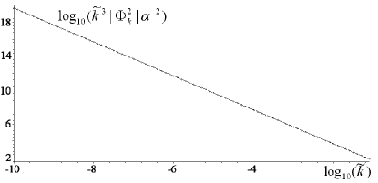
Figure 1: The numerical integration of (42) yields the spectrum (43) evaluated at $x=1/(4\tilde{k})$ (dots); the solid line corresponds to a spectral index of $n_{s}=-1$, in agreement with the analytic result (67). Higher order effects in $\tilde{k}$ are accounted for by letting $\tilde{k}$ cover a broad range from $1$ down to $10^{-10}$.

III.4 Interpretation

Our result of the previous section clearly shows that for the specific bouncing cosmology considered, both modes (the initial constant one and the growing one) will pass through the bounce, but it is the mode with the redder spectrum, i.e. the growing mode for the Bunch-Davis vacuum, that dictates the final shape of the post-bounce spectrum. Henceforth, we observe mode mixing in a model with only one degree of freedom and no spatial curvature. One has to be more careful to draw such conclusion for more general cases involving two different fluids (constrained by an adiabatic condition in other backgrounds), since the matching procedure at $\pm\tilde{x}$ is not that simple in general. To be more specific, the feature of the bounce which is crucial for determining the approximate behavior of the out coming spectrum, besides knowing the existence and regularity of the solutions throughout the bounce region, is the correction to the equation of motion (56) due to the second fluid. This is the region where modes just turned non oscillatory and corrections due to the bounce have to be considered, because they are crucial for the solution.

Recently, a wide class of bouncing cosmologies with two independent fluids was discussed in Bozza:2005wn ; Bozza:2005xs by Bozza and Veneziano . One might think that, in their notation, our class of bouncing universes corresponds to $\alpha=0$, $c_{a}^{2}=(n-3)/3$, $c_{b}^{2}=2n/3-1=2c_{a}^{2}+1$ and $n=4$. This would put it into region C of Bozza:2005wn and a spectral index of

$$n_{s} = \frac{4(n-3)}{n-1}+1$$ (84)

$$= 3$$ (85)

would result according to Bozza:2005wn . However the model of Bozza:2005wn differs from our bouncing universe, since $\alpha=0$ only enforces the adiabatic condition on each fluid separately and while no intrinsic entropy modes for each fluid are considered, two independent initial conditions for each of these fluids are assumed. In our model the ”two fluids” are indeed related, so that the total pressure becomes a function of the total energy (as a consequence only one initial condition can be specified). In other words, we have enforced the adiabatic condition in its strong interpretation. It should also be noted, the approximation scheme employed there, differs considerably from ours, involving an expansion in $k$ and a dimensional argument for the contribution of the bounce (no explicit solution for the bounce was used). Henceforth, the results of Bozza:2005wn ; Bozza:2005xs can not be applied to our model.

A few words regarding Ekpyrotic/Cyclic scenarios are needed: in Khoury:2001wf ; Khoury:2001bz ; Steinhardt:2001st there is a mechanism present that generates a scale invariant spectrum before the bounce Gratton:2003pe . It was shown in Creminelli:2004jg , that this spectrum will not get transferred to the post-bounce era, if perturbations evolve independently of the details of the bouncing phase. Furthermore, the main conclusion of Bozza:2005wn ; Bozza:2005xs was, that a smooth bounce in four dimensions is not able to generate a scale invariant spectrum via the mode mixing technique. However, all these arguments were specific to bouncing cosmologies in four dimensional gravity. So far, the effective four dimensional description breaks down for all proposed cyclic models Tolley:2003nx near the bounce, and the bounce itself is singular Turok:2004gb ; Battefeld:2004mn . Thus, it is of prime interest to search for a fully regularized bounce in cyclic/ekpyrotic models of the universe, so that one can compute the spectrum of perturbations explicitly in a full five dimensional setting - see e.g. Battefeld:2005wv for a recent proposal and McFadden:2005mq for an argument that mode mixing can occur in the full five dimensional setup. Our results confirm that it is challenging for such a model to succeed, but not impossible.

IV Vector perturbations

Vector perturbations (VP) have recently caught attention in the context of bouncing cosmologies, due to their growing nature in a contracting universe Battefeld:2004cd ; Giovannini:2004mc . In the context of a regularized bounce that we are discussing, VP remain finite and well behaved, as we shall see now.

The most general perturbed metric including only VP is given by Bardeen:1980kt ; Mukhanov:1990me

$$(\delta g_{\mu\nu}) = -a^{2}\left(\begin{array}[]{cc}0&-S^{i}\\ -S^{i}&F^{i}_{\,\,,j}+F^{j}_{\,\,,i}\end{array}\right)\,,$$ (88)

where the vectors $S$ and $F$ are divergenceless, that is $S^{i}_{\,\,,i}=0$ and $F^{i}_{\,\,,i}=0$.

A gauge invariant VP can be defined as Battefeld:2004cd

$$\sigma^{i} = S^{i}+F^{i\,\prime}\,.$$ (89)

The most general perturbation of the energy momentum tensor including only VP is given by Bardeen:1980kt

$$(\delta T^{\mu}_{\,\,\nu}) = \left(\begin{array}[]{cc}0&(\rho_{0}+p_{0})V^{i}\\ -(\rho_{0}+p_{0})(V^{i}+S^{i})&-p_{0}(\pi^{i}_{\,\,,j}+\pi^{j}_{\,\,,i})\end{array}\right)\,,$$ (92)

where $\pi^{i}$ and $V^{i}$ are divergenceless. Furthermore the perturbation in the 4-velocity is related to $V^{i}$ via

$$(\delta u^{\mu})=\left(\begin{array}[]{c}0\\ \frac{V^{i}}{a}\end{array}\right)\,.$$ (96)

Gauge invariant quantities are given by

$$\theta^{i} = V^{i}-F^{i\,\prime}$$ (97)

and $\pi^{i}$.

From now on we work in Newtonian gauge, where $F^{i}=0$ so that $\sigma$ coincides with $S$ and $\theta$ with $V$. Note that there is no residual gauge freedom after going to Newtonian gauge. For simplicity we assume the absence of anisotropic stress, $\pi^{i}=0$, so that

$$(\delta S^{\mu}_{\,\,\nu}) = \frac{1}{6}\rho_{0}\left(\begin{array}[]{cc}0&(\rho+p)V^{i}\\ -(\rho+p)(V^{i}+S^{i})&0\end{array}\right)\,.$$ (100)

The resulting equations of motion read

$$\frac{1}{2a^{2}}\nabla^{2}S^{i} = -\kappa^{2}\rho_{0}(1+w)\left(1-\frac{\rho_{0}}{\lambda}\right)V^{i}\,,$$ (102)

$$0 = -\frac{1}{2a^{4}}\partial_{\eta}\left(a^{2}\left(S^{j}_{\,\,,i}+S^{i}_{\,\,,j}\right)\right)\,.$$ (103)

Equation (103) is easily intergrated for each Fourier mode, yielding

$$S_{(k)}^{i}=\frac{C_{(k)}^{i}}{a^{2}}\,,$$ (104)

where $C_{(k)}^{i}$ is time independent. Since $a>0$, there is no divergent mode present. Equation (102) is an algebraic equation for each Fourier mode of the velocity perturbation $V^{i}$. Since $(1-\rho_{0}/\lambda)$ becomes zero shortly before and after the bounce, it seems like $V^{i}$ has to diverge before the bounce – however, all that this is telling us is that $V^{i}$ is not the right variable to focus on: we should focus on the combination of $V^{i}$ and $\rho_{0}$ that appears in the perturbation of the effective total energy momentum tensor, that is $\rho_{0}(1+w)\left(1-\rho_{0}/\lambda\right)V^{i}$. This combination is well behaved, and in fact one can check that it is always smaller than either $\rho_{+}-\rho_{-}$ or $p_{+}-p_{-}$ if we impose appropriately small initial conditions for $C_{(k)}^{i}$. Thus the perturbative treatment of VP is consistent.

V Tensor perturbations

In this section we calculate the amplitude and spectral index of gravity waves , corresponding to tensor perturbations of the metric, in a radiation dominated universe. Because the complete five dimensional calculation is very complicated we will continue using the theory of linear perturbations in a four dimensional effective field theory. We include only the corrections $\propto S^{\mu}_{\,\nu}$, due to fifth dimension, entering through the evolution of the background.

In the linear theory of cosmological perturbations, tensor perturbations can be added to the background metric via Mukhanov:1990me

$$ds^{2}=a^{2}[d\eta^{2}-(\delta_{ij}+h_{ij})dx^{i}dx^{j}]\,,$$ (105)

where $h_{ij}$ has to satisfy

$$h^{i}_{i}=h^{|j}_{ij}=0\,.$$ (106)

Thus $h_{ij}$ has only two degrees of freedom which correspond to the two polarizations of gravity waves. One can show (see Mukhanov:1990me ) that the amplitude $h$ for each of these polarizations has to obey

$$\mu^{\prime\prime}-\nabla^{2}\mu-{a^{\prime\prime}\over a}\mu=0\,,$$ (107)

where $\mu=ah$. Note that gravity waves do not couple to energy or pressure and that they are gauge invariant from the start.

If the second term dominates over ${\mu a^{\prime\prime}/a}$ in the above equation $\mu$ will exhibit oscillatory solutions, and if the gradient term is negligible we will have $\mu\sim a$, or, in other words, $h$ is almost constant. Using the standard Fourier decomposition we get for each Fourier mode

$$\mu_{k}^{\prime\prime}+\left(k^{2}-{a^{\prime\prime}\over a}\right)\mu_{k}=0\,.$$ (108)

Therefore, ${a^{\prime\prime}/a}$ sets a scale for the behavior of each mode. This is very similar to the role of the Hubble radius for inflationary scenarios, but rather than being almost constant, ${a^{\prime\prime}/a}$ is more like a potential barrier in quantum mechanics:

$${\cal V}(x):=\left({t_{0}\over a_{0}}\right)^{2}{a^{\prime\prime}\over a}={1\over 2}{1\over(1+x^{2})^{3/2}}\,.$$ (109)

As Fig. 2 shows, ${\cal V}(x)$ rises up to ${1\over 2}$ around the bounce but falls off very quickly as $x\rightarrow\pm\infty$.

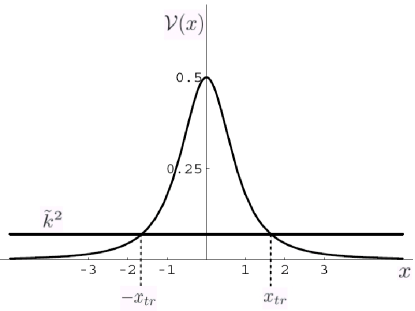
Figure 2: ${\cal V}(x)$ sets a scale for the behavior of each mode, it rises up to ${1\over 2}$ around the bounce but falls off very quickly as $x\rightarrow\pm\infty$.

Thus, for $\tilde{k}^{2}\gg{1\over 2}$, the solutions of equation (108) are oscillatory. This implies that we can set our initial conditions according to the Bunch-Davis vacuum at the initial time $\eta_{i}$. We get

$$\mu_{k}(\eta)={1\over\sqrt{2k}}e^{-ik(\eta-\eta_{i})}\,,$$ (110)

long before the bounce and it will remain basically unchanged throughout the bounce. We easily compute the spectrum of perturbations and the spectral index for these modes to be

$${\mathcal{P}}_{k} := {2k^{3}\over M_{p}^{2}a^{2}}\left|\mu_{k}^{2}\right|={2k^{2}\over M_{p}^{2}a^{2}}\propto k^{n_{t}}\,,$$ (111)

$$n_{t} = 2~{}.$$ (112)

implying that, for $\tilde{k}^{2}\gg{1\over 2}$, we are simply left with vacuum fluctuations with an ever decaying amplitude.

Let us now turn our attention to the more interesting case: $\tilde{k}^{2}\ll{1\over 2}$. As Fig. 2 demonstrates for these modes, we have transitions from the regime $\tilde{k}^{2}\gg{\cal V}(x)$ (i.e. $k^{2}\gg{a^{\prime\prime}/a}$) to the regime $\tilde{k}^{2}\ll{\cal V}(x)$ at the transition points $\pm x_{{}_{tr}}$($\pm\eta_{{}_{tr}}$). Here $x_{{}_{tr}}$ ($\eta_{{}_{tr}}$) is taken to be positive and using (109) we get

$$x_{{}_{tr}}\simeq 2^{-1/3}~{}\tilde{k}^{-2/3}\,.$$ (113)

For $|x|\gg x_{{}_{tr}}$ ($|\eta|\gg\eta_{{}_{tr}}$) we can simply approximate the solutions of equation (108) to be oscillatory

$$\mu_{k}(\eta) = {1\over\sqrt{2k}}[A_{1}e^{-ik(\eta-\eta_{i})}+B_{1}e^{ik(\eta-\eta_{i})}\bigl{]}\,,~{}~{}~{}\eta\ll-\eta_{{}_{tr}}$$

$$\mu_{k}(\eta) = {1\over\sqrt{2k}}\bigr{[}A_{3}e^{-ik\eta}+B_{3}e^{ik\eta}\bigl{]}\,,~{}~{}~{}\eta\gg\eta_{{}_{tr}}$$ (115)

where $A_{1}$ and $B_{1}$ are constants set by initial conditions. In the case of the Bunch-Davis vacuum we can set $A_{1}=1$ and $B_{1}=0$. We will derive $A_{3}$ and $B_{3}$ by matching the solutions smoothly at the transition points.

But first, we need to estimate the solutions for $\tilde{k}^{2}\ll{\cal V}(x)$ (i.e. $k^{2}\ll{a^{\prime\prime}/a}$) that is for $|x|\ll x_{{}_{tr}}$. Unfortunately, unlike the case of most potential barriers in Quantum Mechanics, we can not use the WKB approximation to calculate the outgoing spectrum, since the condition

$${\partial(k^{2}-a^{\prime\prime}/a)/\partial\eta\over(k^{2}-a^{\prime\prime}/a)^{2}}\ll 1$$ (116)

is not satisfied in this regime. Fortunately we can still approximate the solution of equation (108) perturbatevely in orders of $k^{2}$

$${\mu_{k}(\eta)\over a(\eta)} = A_{2}\left[1-k^{2}\int^{\eta}{d\tau\over a^{2}}\int^{\tau}d\varsigma~{}a^{2}\right]$$

$$+B_{2}\int^{\eta}{d\tau\over a^{2}}\left[1-k^{2}\int^{\tau}d\varsigma~{}a^{2}\int^{\varsigma}{d\rho\over a^{2}}\right]+\cdot\cdot\cdot\,.$$

For $|\eta|\approx\eta_{{}_{tr}}$, since

$$\int_{0}^{\infty}{d\eta\over a^{2}} = 2.60{t_{0}\over a_{0}^{3}}\,,$$ (118)

$$a \approx a_{0}|x|^{1/2}\sim a_{0}\tilde{k}^{-1/3}$$ (119)

and also

$$k^{2}\int^{\eta}_{0}{d\tau\over a^{2}}\int^{\tau}_{0}d\varsigma~{}a^{2}\approx{2\over 3}\,\tilde{k}^{2}|x|~{}\sim{2\over 3}\tilde{k}^{4/3}\,,$$ (120)

one can further approximate the result of equation (V) to

$$\mu_{k}(x)=A_{2}a_{0}|x|^{1/2}+B_{2}{t_{0}\over a_{0}^{2}}{|x|\over x}[2.6|x|^{1/2}-2]\,.$$ (121)

Notice that $\mu_{k}^{\prime\prime}(\eta_{{}_{tr}})=0$ for the above solution, since

$${d\mu_{k}\over d\eta}={1\over 2}\left[\pm{A_{2}a_{0}^{2}\over t_{0}}+2.60{B_{2}\over a_{0}}\right]\sim\rm{Const.}$$ (122)

at $|\eta|\approx\eta_{{}_{tr}}$. Therefore, $\mu_{k}$ can be smoothly matched to our solutions from equations (LABEL:solutionI) and (115) at the transition points $\pm x_{{}_{tr}}$ by equating $\mu_{k}$ and $\mu_{k}^{\prime}$. We obtain the transfer function by relating the coefficients $A_{1}$ and $B_{1}$ to $A_{3}$ and $B_{3}$. These satisfy the relations

$$A_{3} \simeq e^{ik(2\eta_{{}_{tr}}+\eta_{i})}\bigl{[}0.65~{}i\tilde{k}^{-1}+2.32\tilde{k}^{-1/3}\bigr{]}A_{1}$$

$$+e^{-ik\eta_{i}}[0.65~{}i\tilde{k}^{-1}]B_{1}\,,$$

$$B_{3} \simeq e^{ik\eta_{i}}[-0.65~{}i\tilde{k}^{-1}]A_{1}$$

$$+e^{-ik(2\eta_{{}_{tr}}+\eta_{i})}\bigl{[}-0.65~{}i\tilde{k}^{-1}+2.32\tilde{k}^{-1/3}\bigr{]}B_{1}\,.$$

The above result is valid for general initial conditions. We first note that, to lowest order in $k^{-1}$, the constant mode in the pre-collapse phase (growing mode for h), matches onto the growing mode in the post-collapse phase (constant mode for h), without any change in the spectral shape. As we mentioned before, for a Bunch-Davis vacuum one simply takes $A_{1}=1$ and $B_{1}=0$. The resulting power-spectrum for such a case is

$${\cal P}_{k}=13.44\left({\tilde{M}_{p}\over M_{p}}\right)^{6}~{}x^{-1}\sin^{2}\left(k(\eta-\eta_{{}_{tr}})\right)\,.$$ (125)

The above spectrum is oscillatory and, for $k(\eta-\eta_{{}_{tr}})\gg 1$, it is oscillating so fast that one could conclude an almost flat ($n_{t}=0$) effective spectrum, with a decaying amplitude. However, if $k(\eta-\eta_{{}_{tr}})\ll 1$ or in other words $1\ll x\ll 1/(4\tilde{k}^{2})$, which is the case for super-Hubble wavelengths, the above equation simplifies to

$${\cal P}_{k}=53.76\left({\tilde{M}_{p}\over M_{p}}\right)^{6}\tilde{k}^{2}\,.$$ (126)

Thus, we get a non-decaying mode which has a blue spectrum ($n_{t}=2$). Notice, the amplitude of the power spectrum was dictated directly by the scales and details of the bounce. This result is in agreement with the conclusions of Martin:2001ue , where a scale factor somewhat similar to our background scale factor was used.

VI Conclusion

We constructed a wide class of regular bouncing universes, with a smooth transition from contraction to expansion. This was motivated by open questions regarding the evolution of perturbations during singular bouncing cosmologies in string cosmology, occurring e.g. in the cyclic scenario. The bounce is caused by the presence of an extra time-like dimension, which introduces corrections to the effective four dimensional Einstein equations at large energy densities. If matter respecting the null energy condition is present, a big bang avoiding bounce results, and for phantom matter a big rip avoiding bounce emerges. We find analytic expressions for the scale factor in all cases.

Having the Cyclic scenario in mind, we focused on a specific big bang avoiding bounce with radiation as the only matter component. We then discussed linear scalar, vector and tensor perturbations.

For scalar perturbations we compute analytically a spectral index of $n_{s}=-1$, thus ruling out such a model as a realistic candidate. We also find the spectrum to be sensitive to the bounce region, in agreement to the majority of regular toy models discussed in the literature. We conclude that it is challenging, but not impossible, for Cyclic/Ekpyrotic models to succeed, if one can find a regularized version.

Next, we discussed vector perturbations which are known to be problematic in bouncing cosmologies, due to their growing nature. We checked explicitly that they remain perturbative and small if compared to the background energy density and pressure.

We concluded with a discussion of gravitational waves. The transfer function was computed analytically and we showed that the shape of the spectrum is unchanged in general. In the special case of vacuum initial conditions, the spectral index in post bounce era for super-Hubble wavelengths is blue. However, the amplitude turned out to be sensitive to the details of our model.

To summarize, having an explicit realization of e.g. the Cyclic model of the universe that features a regular bounce it might be possible to produce a scale invariant spectrum. Henceforth, the challenge for the Cyclic model is twofold:

1. To find a convincing mechanism that regularizes the bounce.

2. To deal with the perturbations in a full five dimensional setup and to take into account the presence of an inhomogeneous bulk as inevitable by the presence of branes.

Preliminary results show that, by incorporating ideas of string/brane gas cosmology (see Brandenberger:2005fb ; Brandenberger:2005nz ; Battefeld:2005av for recent reviews), a regularized bounce is possible (in preparation).

- (1) J. E. Lidsey, D. Wands and E. J. Copeland, Phys. Rept. 337, 343 (2000) [arXiv:hep-th/9909061].
- (2) J. Khoury, B. A. Ovrut, P. J. Steinhardt and N. Turok, Phys. Rev. D 64, 123522 (2001) [arXiv:hep-th/0103239].
- (3) J. Khoury, B. A. Ovrut, N. Seiberg, P. J. Steinhardt and N. Turok, Phys. Rev. D 65, 086007 (2002) [arXiv:hep-th/0108187].
- (4) P. J. Steinhardt and N. Turok, Phys. Rev. D 65, 126003 (2002) [arXiv:hep-th/0111098].
- (5) S. Gratton, J. Khoury, P. J. Steinhardt and N. Turok, Phys. Rev. D 69, 103505 (2004) [arXiv:astro-ph/0301395].
- (6) A. J. Tolley, N. Turok and P. J. Steinhardt, Phys. Rev. D 69, 106005 (2004) [arXiv:hep-th/0306109].
- (7) M. Gasperini and G. Veneziano, Astropart. Phys. 1, 317 (1993) [arXiv:hep-th/9211021].
- (8) M. Gasperini and G. Veneziano, Phys. Rept. 373, 1 (2003) [arXiv:hep-th/0207130].
- (9) T. J. Battefeld, S. P. Patil and R. Brandenberger, Phys. Rev. D 70, 066006 (2004) [arXiv:hep-th/0401010].
- (10) N. Turok, M. Perry and P. J. Steinhardt, Phys. Rev. D 70, 106004 (2004) [Erratum-ibid. D 71, 029901 (2005)] [arXiv:hep-th/0408083].
- (11) J. Khoury, B. A. Ovrut, P. J. Steinhardt and N. Turok, Phys. Rev. D 66, 046005 (2002) [arXiv:hep-th/0109050].
- (12) R. Durrer and F. Vernizzi, Phys. Rev. D 66, 083503 (2002) [arXiv:hep-ph/0203275].
- (13) J. Martin, P. Peter, N. Pinto-Neto and D. J. Schwarz, Phys. Rev. D 65, 123513 (2002) [arXiv:hep-th/0112128].
- (14) R. Brandenberger and F. Finelli, JHEP 0111, 056 (2001) [arXiv:hep-th/0109004].
- (15) N. Goheer, P. K. S. Dunsby, A. Coley and M. Bruni, arXiv:hep-th/0408092.
- (16) P. Peter and J. Martin, arXiv:hep-th/0402081.
- (17) J. Martin and P. Peter, Phys. Rev. D 68, 103517 (2003) [arXiv:hep-th/0307077].
- (18) L. E. Allen and D. Wands, Phys. Rev. D 70, 063515 (2004) [arXiv:astro-ph/0404441].
- (19) P. Peter and N. Pinto-Neto, Phys. Rev. D 66, 063509 (2002) [arXiv:hep-th/0203013].
- (20) V. Bozza and G. Veneziano, Phys. Lett. B 625, 177 (2005) [arXiv:hep-th/0502047].
- (21) V. Bozza and G. Veneziano, JCAP 0509, 007 (2005) [arXiv:gr-qc/0506040].
- (22) V. Bozza, arXiv:hep-th/0512066.
- (23) F. Finelli, JCAP 0310, 011 (2003) [arXiv:hep-th/0307068].
- (24) C. Cartier, arXiv:hep-th/0401036.
- (25) T. J. Battefeld and G. Geshnizjani, arXiv:hep-th/0506139, to appear in PRD, comments.
- (26) M. Gasperini, M. Giovannini and G. Veneziano, Phys. Lett. B 569, 113 (2003) [arXiv:hep-th/0306113].
- (27) M. Gasperini, M. Giovannini and G. Veneziano, Nucl. Phys. B 694, 206 (2004) [arXiv:hep-th/0401112].
- (28) A. Linde, arXiv:hep-th/0205259.
- (29) D. N. Spergel et al. [WMAP Collaboration], Astrophys. J. Suppl. 148, 175 (2003) [arXiv:astro-ph/0302209].
- (30) Patrick Peter, Nelson Pinto-Neto, Diego A. Gonzalez, JCAP 0312:003,2003. [HEP-TH 0306005]
- (31) R. Brandenberger, V. Mukhanov and A. Sornborger, Phys. Rev. D 48, 1629 (1993) [arXiv:gr-qc/9303001].
- (32) S. Tsujikawa, R. Brandenberger and F. Finelli, Phys. Rev. D 66, 083513 (2002) [arXiv:hep-th/0207228].
- (33) L. Randall and R. Sundrum, Phys. Rev. Lett. 83, 3370 (1999) [arXiv:hep-ph/9905221].
- (34) P. Brax, C. van de Bruck and A. C. Davis, arXiv:hep-th/0404011.
- (35) Y. Shtanov and V. Sahni, Phys. Lett. B 557, 1 (2003) [arXiv:gr-qc/0208047].
- (36) M. G. Brown, K. Freese and W. H. Kinney, arXiv:astro-ph/0405353.
- (37) Y. S. Piao and Y. Z. Zhang, arXiv:gr-qc/0407027.
- (38) G. R. Dvali, G. Gabadadze and G. Senjanovic, arXiv:hep-ph/9910207.
- (39) S. Matsuda and S. Seki, Nucl. Phys. B 599, 119 (2001) [arXiv:hep-th/0008216].
- (40) M. Chaichian and A. B. Kobakhidze, Phys. Lett. B 488, 117 (2000) [arXiv:hep-th/0003269].
- (41) I. Bars, arXiv:hep-th/0106021.
- (42) T. Shiromizu, K. I. Maeda and M. Sasaki, Phys. Rev. D 62, 024012 (2000) [arXiv:gr-qc/9910076].
- (43) R. Maartens, Phys. Rev. D 62, 084023 (2000) [arXiv:hep-th/0004166].
- (44) S. Nojiri and S. D. Odintsov, Phys. Rev. D 70, 103522 (2004) [arXiv:hep-th/0408170].
- (45) J. M. Bardeen, Phys. Rev. D 22, 1882 (1980).
- (46) V. F. Mukhanov, H. A. Feldman and R. H. Brandenberger, Phys. Rept. 215, 203 (1992).
- (47) R. H. Brandenberger, arXiv:hep-th/0501033.
- (48) M. Abramowitz and I. Stegun, Handbook of Mathematical Functions, (Dover Publ., New York, 1985).
- (49) P. Creminelli, A. Nicolis and M. Zaldarriaga, arXiv:hep-th/0411270.
- (50) M. Giovannini, arXiv:hep-th/0502068.
- (51) T. J. Battefeld, S. P. Patil and R. H. Brandenberger, arXiv:hep-th/0509043, to appear in PRD.
- (52) P. McFadden, N. Turok and P. J. Steinhardt, arXiv:hep-th/0512123.
- (53) T. J. Battefeld and R. Brandenberger, Phys. Rev. D 70, 121302(R) (2004) [arXiv:hep-th/0406180].
- (54) M. Giovannini, Phys. Rev. D 70, 103509 (2004) [arXiv:hep-th/0407124].
- (55) A. A. Starobinsky, JETP Lett. 30, 682 (1979) [Pisma Zh. Eksp. Teor. Fiz. 30, 719 (1979)].
- (56) R. H. Brandenberger, arXiv:hep-th/0509099.
- (57) R. H. Brandenberger, arXiv:hep-th/0509159.
- (58) T. Battefeld and S. Watson, arXiv:hep-th/0510022, to appear in Rev. Mod. Phys.