SNUST-050301 ROM2F/2005/04 hep-th/0503148

D-branes in a Big Bang/Big Crunch Universe:

Nappi-Witten Gauged WZW Model

Yasuaki Hikida,^a Rashmi R. Nayak^b and Kamal L. Panigrahi^b

^a School of Physics & BK-21 Physics Division, Seoul National University

Seoul 151-747, Korea

^b Dipartimento di Fisica & INFN, Sezione di Roma 2, “Tor Vergata”,

Roma 00133, Italy

We study D-branes in the Nappi-Witten model, which is a gauged WZW model based on $(SL(2,\mathbb{R})\times SU(2))/(U(1)\times U(1))$. The model describes a four dimensional space-time consisting of cosmological regions with big bang/big crunch singularities and static regions with closed time-like curves. The aim of this paper is to investigate by D-brane probes whether there are pathologies associated with the cosmological singularities and the closed time-like curves. We first classify D-branes in a group theoretical way, and then examine DBI actions for effective theories on the D-branes. In particular, we show that D-brane metric from the DBI action does not include singularities, and wave functions on the D-branes are well behaved even in the presence of closed time-like curves.

1 Introduction

The formulation of string theory in cosmological or broadly time-dependent backgrounds still remains as one of the most exciting open challenges for theoretical physicists. Among other things, it is important to see how (whether) string theory resolves the cosmological singularities (or not). Some recent attempts along this direction have been made in [1, 2, 3, 4, 5, 6, 7, 8, 9, 10, 11, 12, 13]. In this paper, we investigate the Nappi-Witten (NW) model [14, 15] as a conformal field theory (CFT) model that includes big bang and big crunch singularities. This model is defined as an $SL(2,\mathbb{R})\times SU(2)$ WZW model gauged by $U(1)\times U(1)$ in an asymmetric way. Therefore we can solve it exactly and gain some understanding of the behaviour of strings across these singularities. Similar attempts have been made to understand the cosmological backgrounds by using gauged WZW models, e.g., in [16, 17, 18, 19, 20].

The NW model describes a four dimensional anisotropic universe that starts at a big bang singularity, expands for a while, ends at a big crunch singularity within a finite affine time, and again starts at another big bang singularity. It was argued in [15] that strings across these singularities make sense because the theory is defined as a coset CFT. This may be related to the fact that strings have a finite length scale $l_{s}$ and may go through the singularities. As described in [15], the coset contains, in addition to copies of the cosmological regions, non-compact and time independent (static) regions known as whiskers. The whisker part of the full space-time contains closed time-like curves (CTCs), which seems to be unacceptable for any measurable quantity like S-matrix. Nevertheless, these CTCs are argued to be necessary for defining the observables in terms of gauged WZW model [15].

Hence we would like to ask a question, whether studying the dynamics of D-branes sheds more lights on the understanding of big bang/big crunch singularities and CTCs. This is a non-trivial question because the D-branes, or the open strings ending on them, feel the background geometry in a different way. In particular, D0-brane is an useful candidate to probe the singularities, because the point particle could probe directly the singular points. In fact, the singularities are at strong coupling regions, thus D-branes may serve as more effective probes than strings. Moreover, we might expect that the effective theories on D-branes wraping the CTCs include pathologies associated with CTCs. This is an analogous situation to D-branes in a supersymmetric Gödel-type universe [21].

The organization of the paper is as follows. In section 2, we review the geometry of the quotient CFT background $(SL(2,{\mathbb{R}})\times SU(2))/(U(1)\times U(1))$ [14, 15], where we fix the notation and summarize the properties of the geometry. In section 3, we investigate D-branes in the cosmological regions. Branes in the coset theory are constructed to descend from maximally symmetric and symmetry breaking branes in $SL(2,\mathbb{R})\times SU(2)$ WZW models [29, 30]. We use the DBI analysis to investigate by D-brane probes the geometry especially near the singularities. In particular, we show that the singularities are cancelled in the DBI action, so the D-brane metric does not include singularities. We also find that the classical solutions reproduce the group theoretic results. In section 4, we investigate D-branes in the whisker regions. The trajectories of the D-branes are also classified in a group theoretical way, and the DBI action is used to probe the geometry by the branes. Open string spectrum on the D-brane wrapping CTCs can be read off from the eigenfunction of Laplacian in terms of open string metric and open string coupling [31]. We see that the spectrum does not include any pathology associated with CTCs. Section 5 is devoted to a detailed study of the wave functions in various sectors of the model. Finally, we conclude in section 6 with discussions and some open questions. Appendix A includes a brief analysis on D-branes in Misner space-time.

2 Background geometry

In general it is difficult to analyze string theory in cosmological backgrounds. However, the gauged WZW models are few techniques to construct exact string models for cosmological systems (see, e.g., [16, 17, 14, 15, 18, 19, 20]). In this paper, we investigate a coset model proposed by Nappi and Witten [14], which describes a four dimensional anisotropic, expanding and contracting closed universe. The coset that we are interested in is $SL(2,\mathbb{R})\times SU(2)$ WZW model with the following identification

$$(g,g^{\prime})\sim(e^{\rho\sigma_{3}}ge^{\tau\sigma_{3}},e^{i\tau\sigma_{3}}g^{\prime}e^{i\rho\sigma_{3}}),$$ (2.1)

where we denote $g,g^{\prime}$ as elements of $SL(2,\mathbb{R})$ and $SU(2)$, respectively. The levels $k,k^{\prime}$ for the $SL(2,\mathbb{R})$ and $SU(2)$ WZW models are set to be equal $(k=k^{\prime})$, and they are considered to be large because we are interested in the classical properties. A critical bosonic string theory should include extra space dimensions such that the total central charge $c=26$. The extension to the superstring case should be straightforward.

Figure 1: A two-dimensional sketch of the four-dimensional space-time. Regions $I-IV$ represent closed universe regions with the singularities at the beginning and at the end. Regions $1-4$ and $1^{\prime}-4^{\prime}$ are the whisker regions which contain closed time-like curves.

As we will see below, the NW model includes twelve regions as in fig. 1. It originates from the fact that our parametrization of $SL(2,\mathbb{R})$ is divided into twelve cases, depending on the signs of its group elements. We find it convenient to represent, inside each regions, the most general group element $g\in SL(2,\mathbb{R})$ as

$$g =e^{\alpha\sigma_{3}}(-1)^{\epsilon_{1}}(i\sigma_{2})^{\epsilon_{2}}g_{\delta}(\theta)e^{\beta\sigma_{3}},$$ (2.2)

where $\alpha,\beta\in\mathbb{R}$ and $\epsilon_{1},\epsilon_{2}=0,1$. If we set $\epsilon_{1}=\epsilon_{2}=0$, then the parameters are in region $\delta=II,1,1^{\prime}$ with

$$g_{II} =\begin{pmatrix}\cos\theta&\sin\theta\\ -\sin\theta&\cos\theta\end{pmatrix}, g_{1} =g_{1^{\prime}}^{-1}=\begin{pmatrix}\cosh\theta&\sinh\theta\\ \sinh\theta&\cosh\theta\end{pmatrix}.$$ (2.3)

The parameter $\theta$ runs from $0~{}{\rm to}~{}\pi/2~{}(0\leq\theta\leq\pi/2)$ in region II and $\theta\geq 0$ in regions $1$ and $1^{\prime}$. We obtain, in total, twelve regions by changing $\epsilon_{1,2}=0,1$, however it is evident that the change of $\epsilon_{1,2}$ does not affect the value of the quantity

$$W={\rm Tr}(\sigma_{3}g\sigma_{3}g^{-1}).$$ (2.4)

(A)	$W>2$	$1\begin{pmatrix}\ +&+\\ +&+\end{pmatrix}$	$1^{\prime}\begin{pmatrix}\ +&-\\ -&+\end{pmatrix}$	$3\begin{pmatrix}\ -&-\\ -&-\end{pmatrix}$	$3^{\prime}\begin{pmatrix}\ -&+\\ +&-\end{pmatrix}$
(B)	$-2<W<2$	$I\begin{pmatrix}\ +&-\\ +&+\end{pmatrix}$	$II\begin{pmatrix}\ +&+\\ -&+\end{pmatrix}$	$III\begin{pmatrix}\ -&+\\ -&-\end{pmatrix}$	$IV\begin{pmatrix}\ -&-\\ +&-\end{pmatrix}$
(C)	$W<-2$	$2\begin{pmatrix}\ -&+\\ -&+\end{pmatrix}$	$2^{\prime}\begin{pmatrix}\ +&+\\ -&-\end{pmatrix}$	$4\begin{pmatrix}\ +&-\\ +&-\end{pmatrix}$	$4^{\prime}\begin{pmatrix}\ -&-\\ +&+\end{pmatrix}$

Table 1: Twelve regions for the parametrization of $g\in SL(2,\mathbb{R})$.

In other words, we can separate the twelve regions into three types as in table 1. In type (B), the parameter $\theta$ in regions $III,IV,$ and $I$ may be obtained by shifting $\theta\to\theta+n\pi/2$ with $n=1,2,3$. For $A$ and $A^{\prime}$ with $A=1,2,3,4$, we may replace $\theta$ by $-\theta$. Moreover, regions 1 and 3, or regions 2 and 4 are different only with the overall factor $g\to-g$.

Similarly, for $g^{\prime}\in SU(2)$ we can use for all the regions

$$g^{\prime}=e^{i\beta^{\prime}\sigma_{3}}e^{i\phi\sigma_{2}}e^{i\alpha^{\prime}\sigma_{3}}$$ (2.5)

with $\alpha^{\prime}\sim\alpha^{\prime}+2\pi,\beta^{\prime}\sim\beta^{\prime}+2\pi$ and $0\leq\phi\leq\pi/2$. Even so, we adopt a bit different way of parametrization in order to express the metric in a simpler form as we see below. Moving into the regions $III,IV,$ and $I$, we change $\phi$ into $\phi\to\phi+n\pi/2$ $(n=1,2,3)$ and shift the region into $-n\pi/2<\phi<(1-n)\pi/2$. The same thing should happen when we change $1\to 2\to 3\to 4$ or $1^{\prime}\to 2^{\prime}\to 3^{\prime}\to 4^{\prime}$. From now on, we will concentrate on region $II$, region $1$ and region $2^{\prime}$, since the other regions can be analyzed by using the above transformations.

The geometry of the NW model can be obtained by starting from the $SL(2,\mathbb{R})\times SU(2)$ WZW action and then by integrating out the gauge fields associated with $U(1)\times U(1)$ [14, 15]. The coordinates invariant under the gauge transformation (2.1) are given by $\alpha-\alpha^{\prime}$, $\beta-\beta^{\prime}$, $\theta$, $\phi$. We use a gauge choice $\alpha^{\prime}=\beta^{\prime}=0$ and denote $\alpha\pm\beta=\lambda_{\pm}$. In region $II$, metric, B-field and dilaton are given by

$$ds^{2}=-d\theta^{2}+d{\phi}^{2}+\frac{\cot^{2}\phi}{1+\tan^{2}\theta\cot^{2}\phi}d\lambda^{2}_{+}+\frac{\tan^{2}\theta}{1+\tan^{2}\theta\cot^{2}\phi}d\lambda^{2}_{-},$$

$$B_{\lambda_{-}\lambda_{+}}=\frac{1}{1+\tan^{2}\theta\cot^{2}\phi},\qquad\Phi=\Phi_{0}-\frac{1}{2}\log(\cos^{2}\theta\sin^{2}\phi+\sin^{2}\theta\cos^{2}\phi).$$ (2.6)

The time coordinate is given by $\theta$, which starts at $\theta=0$ and ends at $\theta=\pi/2$. At the beginning $(\theta=0)$, a component of the metric $g_{\lambda_{-}\lambda_{-}}$ vanishes, therefore the volume of the universe also vanishes. We interpret this as the universe starts at $\theta=0$ with a big bang singularity. At the end $(\theta=\pi/2)$, another component of the metric $g_{\lambda_{+}\lambda_{+}}$ becomes zero, so this point may be interpreted as a big crunch singularity. For a general $\phi$, these singularities are of orbifold-type. However, at $\theta=\phi=0$ or $\theta=\phi=\pi/2$, the metric and dilaton field diverge, and these singularities are of the same type as the space-like singularities in the two dimensional black hole [34, 35]. More detailed structure of these singularities in this region can be found in [14]. The ranges of other parameters are $0\leq\phi\leq\pi/2$ and $0\leq\lambda_{\pm}<2\pi$. Note that $\lambda_{\pm}$ are periodic parameters $(\lambda_{\pm}\sim\lambda_{\pm}+2\pi)$ due to the periodicity of the parameters $\alpha^{\prime}~{}{\rm and}~{}\beta^{\prime}$. The constant part of the dilaton field will be set to be zero $(\Phi_{0}=0)$ for simplicity.

As we will see later, wave functions are given as eigenfunctions of Laplacian, which is given by

$$\Delta=\frac{1}{e^{-2\Phi}\sqrt{-g}}\partial_{\mu}e^{-2\Phi}\sqrt{-g}g^{\mu\nu}\partial_{\nu}$$ (2.7)

in a general curved background. The Laplacian in this region can be computed as

$$\Delta= \left[-\frac{1}{\cos\theta\sin\theta}\partial_{\theta}(\cos\theta\sin\theta)\partial_{\theta}+\tan^{2}\theta\partial_{\lambda_{+}}^{2}+\cot^{2}\theta\partial_{\lambda_{-}}^{2}\right]$$

$$+\left[\frac{1}{\cos{\phi}\sin{\phi}}\partial_{{\phi}}(\cos{\phi}\sin{\phi})\partial_{{\phi}}+\tan^{2}{\phi}\partial_{\lambda_{+}}^{2}+\cot^{2}{\phi}\partial_{\lambda_{-}}^{2}\right],$$ (2.8)

which can be seen as a sum of two contributions coming from $SL(2,\mathbb{R})$ and $SU(2)$ parts. Hence we can examine the wave functions for $SL(2,\mathbb{R})$ and $SU(2)$ parts separately. In particular, we do not expect any peculiar behavior of wave functions at $\theta=\phi=0$ or $\theta=\phi=\pi/2$.

In region 1, metric, B-field and dilaton are given by

$$ds^{2}=d\theta^{2}+d{\phi}^{2}+\frac{\cot^{2}\phi}{1-\tanh^{2}\theta\cot^{2}\phi}d\lambda^{2}_{+}-\frac{\tanh^{2}\theta}{1-\tanh^{2}\theta\cot^{2}\phi}d\lambda^{2}_{-},$$

$$B_{\lambda_{+}\lambda_{-}}=\frac{1}{1-\tanh^{2}\theta\cot^{2}\phi},\qquad\Phi=-\frac{1}{4}\log(\cosh^{2}\theta\sin^{2}\phi-\sinh^{2}\theta\cos^{2}\phi)^{2}.$$ (2.9)

The ranges of parameters are $0\leq\theta$, $0\leq\phi\leq\pi/2$ and $0\leq\lambda_{\pm}<2\pi$. Because of the periodicity condition on $\lambda_{\pm}$, there are always CTCs in this region. It is important to note that there is a singular surface along the line

$$1=\tanh^{2}\theta\cot^{2}\phi,$$ (2.10)

which may be seen as a domain wall, and across this line the time coordinate is exchanged between $\lambda_{+}$ and $\lambda_{-}$. Despite the complexity of the structure of this region, the Laplacian is given in a rather simple form as

$$\Delta= \left[\frac{1}{\cosh\theta\sinh\theta}\partial_{\theta}(\cosh\theta\sinh\theta)\partial_{\theta}-\tanh^{2}\theta\partial_{\lambda_{+}}^{2}-\coth^{2}\theta\partial_{\lambda_{-}}^{2}\right]$$

$$+\left[\frac{1}{\cos{\phi}\sin{\phi}}\partial_{{\phi}}(\cos{\phi}\sin{\phi})\partial_{{\phi}}+\tan^{2}{\phi}\partial_{\lambda_{+}}^{2}+\cot^{2}{\phi}\partial_{\lambda_{-}}^{2}\right].$$ (2.11)

In particular, the singular surface (2.10) cannot be seen in this expression. In region $2^{\prime}$, we use the following parametrization

$$g =e^{\alpha\sigma_{3}}\begin{pmatrix}\sinh\theta&\cosh\theta\\ -\cosh\theta&-\sinh\theta\end{pmatrix}e^{\beta\sigma_{3}}.$$ (2.12)

Due to the change of $\phi$, metric, $B$-field and dilation are given by just replacing $\lambda_{+}$ by $\lambda_{-}$ in those for region 1. We should also remember that $\phi$ runs from $-\pi/2~{}{\rm to}~{}0~{}(-\pi/2\leq\phi<0)$.

3 D-branes in the cosmological regions

Let us move to D-branes in the NW model and start from a cosmological region (region $II$). In this region, the background is time-dependent, and hence the energy is not conserved. D-branes in the coset theory are constructed to descend from maximally symmetric and symmetry breaking D-branes in $SL(2,\mathbb{R})\times SU(2)$ WZW model, which are classified by (twisted) conjugacy classes [29, 30]. DBI actions are used to investigate the background geometry, especially near the singularities. We show that the classical solutions reproduce the group theoretical results, and we also examine the wave functions on the D-branes by making use of open string metrics [31].

3.1 Geometry of D-branes: A group theoretic view

Maximally symmetric and symmetry breaking D-branes in WZW models are classified by conjugacy classes and by twisted conjugacy classes, respectively [36, 37, 38, 39, 40]. For these D-branes, holomorphic and anti-holomorphic currents for bulk symmetry are related by linear equations at the worldsheet boundary. Therefore, the corresponding D-branes should be invariant under the symmetry left, which are characterized by (twisted) conjugacy classes. D-branes in coset models can be constructed to descend from these D-branes in a systematic way, for example, as in [41, 42, 43, 44, 45], and for asymmetric cosets including the NW model as in [46, 29, 30]. We obtain the geometry of D-branes using these methods as follows.

We first focus on the conjugacy classes and the twisted conjugacy classes of $SL(2,\mathbb{R})$ and of $SU(2)$. For $SL(2,\mathbb{R})$ part, they are given by

$${\rm A}:\quad{\rm Tr}\,g=2\cosh(\alpha+\beta)\cos\theta=2\kappa,$$ (3.1)

$${\rm B}:\quad{\rm Tr}\,\sigma_{1}g=2\sinh(\alpha-\beta)\sin\theta=2\kappa,$$ (3.2)

where $\kappa\in\mathbb{R}$ and we denote them as A-type and B-type, respectively. The $SL(2,\mathbb{R})$ WZW model describes strings in $AdS_{3}$, and the worldvolumes for A-branes are $H_{2}$ for $0<\kappa<1$, light-cone for $\kappa=1$ and $dS_{2}$ for $\kappa>1$, and that for B-brane is $AdS_{2}$ [47]. Similarly, for $SU(2)$ part, the (twisted) conjugacy class is given by

$${\rm A}:\quad{\rm Tr}\,g^{\prime}=2\cos(\alpha^{\prime}+\beta^{\prime})\cos\phi=2\xi,$$ (3.3)

$${\rm B}:\quad{\rm Tr}\,\sigma_{1}g^{\prime}=-2i\sin(\alpha^{\prime}-\beta^{\prime})\sin\phi=-2i\xi,$$ (3.4)

where $\xi\in\mathbb{R}$ and we call them as A-type and B-type. The twist in the B-type is just an inner automorphism of $SU(2)$ in this case, and hence, in the $SU(2)$ WZW model, the B-brane is obtained by rotating the A-brane. However, in the parafermionic theory $SU(2)/U(1)$, it has been shown that gauging of $U(1)$ part leads to two inequivalent types of D-branes [41, 45].

In order to construct D-branes in the gauged WZW model, we have to take into account of the gauge symmetry. For the purpose, we sum up all the gauge orbits of the (twisted) conjugacy classes, project them into the gauge invariant space, and finally shift by an element of $U(1)\times U(1)$. This procedure is essentially the same as taking the product of conjugacy classes of $SL(2,\mathbb{R})\times SU(2)$ and $U(1)\times U(1)$ as in [30]. Let us call them as XY-type D-brane or XY-brane if they are obtained by descending from X($=$A,B)-type for $SL(2,\mathbb{R})$ part and Y($=$A,B)-type for $SU(2)$ part.

First, let us consider the case of ${\rm Tr}\,g=2\kappa$ and ${\rm Tr}\,g^{\prime}=2\xi$, namely the AA-brane. The conjugacy classes are shifted by the gauge transformation (2.1) as

$$\cosh(\alpha+\beta+\tau+\rho)\cos\theta =\kappa, \cos(\alpha^{\prime}+\beta^{\prime}+\tau+\rho)\cos\phi =\xi.$$ (3.5)

Summing up the orbit we obtain

$$\alpha+\beta-\alpha^{\prime}-\beta^{\prime}=\operatorname*{{\rm arccosh}}\left(\frac{\kappa}{\cos\theta}\right)-\arccos\left(\frac{\xi}{\cos\phi}\right).$$ (3.6)

Therefore the geometry of the D-brane is given by the hypersurface

$$\lambda_{+}-\lambda_{+}^{0}=\operatorname*{{\rm arccosh}}\left(\frac{\kappa}{\cos\theta}\right)-\arccos\left(\frac{\xi}{\cos\phi}\right).$$ (3.7)

Because of the symmetry along $\lambda_{+}$, there is a freedom to shift the total position by $\lambda_{+}^{0}$. Note that we have to sum up $\lambda_{+}^{0}={\lambda_{+}^{0}}^{\prime}+2\pi n$ with $0\leq{\lambda_{+}^{0}}^{\prime}<2\pi,n\in{\mathbb{Z}}$ because of the residual gauge transformation [15], which makes the D-branes travelling in spiral orbits like D0-branes in Misner space (see appendix A). We should notice that $\cos\theta\leq\kappa$ and $\cos\phi\geq|\xi|$. Therefore, there is no brane for $\kappa<0$, instantons at $\theta=\pi/2$ for $\kappa=0$, branes in the time period $\arccos\kappa\leq\theta\leq\pi/2$ for $0<\kappa<1$, and in all the time period $0\leq\theta\leq\pi/2$ for $\kappa\geq 1$. Similarly, there is no brane for $|\xi|>1$, branes at $0\leq\phi\leq\arccos|\xi|$ for $|\xi|<1$ and lower dimensional branes at $\phi=0$ for $\xi=1$. For $\kappa>0$ and $|\xi|<1$, the hypersurface (3.7) describes a D2-brane parametrized by $\theta,\phi$ and $\lambda_{-}$. For $\kappa>0$ and $|\xi|=1$, the corresponding brane is D0-brane at

$$\lambda_{+}-\lambda_{+}^{0}=\operatorname*{{\rm arccosh}}\left(\frac{\kappa}{\cos\theta}\right)$$ (3.8)

and $\phi=0$. Notice that one more dimension is reduced because a component of metric $g_{\lambda_{-}\lambda_{-}}$ is degenerated.

Next, let us move to the case of ${\rm Tr}\,g=2\kappa$ and ${\rm Tr}\,\sigma_{1}g^{\prime}=-2i\xi$, namely the AB-brane. In this case, we sum up the gauge transformation (2.1) of (twisted) conjugacy classes

$$\cosh(\alpha+\beta+\tau+\rho)\cos\theta =\kappa, \sin(\alpha^{\prime}-\beta^{\prime}+\tau-\rho)\sin\phi =\xi,$$ (3.9)

which leads to the restriction of the worldvolume

$$\cos\theta \leq\kappa, \sin\phi \geq|\xi|.$$ (3.10)

As before, there is no brane for $\kappa<0$, instantons at $\theta=\pi/2$ for $\kappa=0$, branes in $\theta\geq\arccos\kappa$ for $0<\kappa<1$, and in all the time for $\kappa\geq 1$. In the case of $\kappa>0$, we have D3-branes for $|\xi|<1$ and D1-branes at $\phi=\pi/2$ for $|\xi|=1$. This type of branes resemble to D1-branes in Misner space explained in appendix A, though D1-branes in Misner space do not have the ends.

Third, we consider the case of ${\rm Tr}\,\sigma_{1}g=2\kappa$ and ${\rm Tr}\,g^{\prime}=2\xi$, namely the BA-brane. In this case, we sum up the gauge transformation (2.1) of (twisted) conjugacy classes

$$\sinh(\alpha-\beta+\tau-\rho)\sin\theta =\kappa, \cos(\alpha^{\prime}+\beta^{\prime}+\tau+\rho)\cos\phi =\xi,$$ (3.11)

which leads to $\cos\phi\geq\xi$. Notice that there is no restriction on the time $\theta$ contrary to the AB-brane case. We have D3-brane for $|\xi|<1$ and D1-brane at $\phi=0$ for $|\xi|=1$.

Final case is ${\rm Tr}\,\sigma_{1}g=2\kappa$ and ${\rm Tr}\,\sigma_{1}g^{\prime}=-2i\xi$, namely the BB-brane. The hypersurface derived from the twisted conjugacy classes is

$$\lambda_{-}-\lambda_{-}^{0}=\operatorname*{{\rm arcsinh}}\left(\frac{\kappa}{\sin\theta}\right)-\arcsin\left(\frac{\xi}{\sin\phi}\right).$$ (3.12)

Again there is no restriction on the time $\theta$. We have D2-brane satisfying (3.12) for $|\xi|<1$ and D0-brane at

$$\lambda_{-}-\lambda_{-}^{0}+\frac{\pi}{2}=\operatorname*{{\rm arcsinh}}\left(\frac{\kappa}{\sin\theta}\right)$$ (3.13)

and $\phi=\pi/2$ for $|\xi|=1$.

3.2 Effective theories on D-branes

The purpose of this paper is to investigate the non-trivial geometry of the NW model using the D-brane probes. In general, D-branes and strings feel the background geometry in different ways, which can be seen from their worldvolume actions. The low energy actions for the worldvolume theories on D-branes are of DBI-type, and D-brane metrics can be read from the effective actions. In this subsection, we construct DBI actions for the D-branes classified in the previous subsection, and see how D-branes feel the background, in particular, near the singularities. We also show that the classical solutions to the equations of motion are consistent with the geometry of D-branes obtained above.

It is also important to examine how the non-trivial background affects open string spectra on the D-branes. A simple way to obtain the low energy spectra for open strings is to utilize open string metrics [31]. Because of non-trivial gauge flux on D-branes, open strings feel the background metric in a modified way. We denote induced closed string metric on D-brane as $g_{ab}$ and closed string coupling as $g_{s}$. Then, open string metric $G_{ab}$ and open string coupling $G_{s}$ in a configuration with ${\cal F}=B+F$ are given by [31]

$$G_{ab} =g_{ab}-{\cal F}_{ac}g^{cd}{\cal F}_{db},$$ (3.14)

$$G_{s}\equiv e^{\Phi_{o}} =g_{s}\sqrt{\frac{-\det G}{-\det(g+{\cal F})}}.$$ (3.15)

The low energy spectra for open strings can be read from the eigenfunctions of Laplacians in terms of open string quantities:

$$\Delta=\frac{1}{e^{-\Phi_{o}}\sqrt{-G}}\partial_{a}e^{-\Phi_{o}}\sqrt{-G}G^{ab}\partial_{b}.$$ (3.16)

In this subsection, we only construct the Laplacians and see their properties. More detailed analysis on wave functions is given in section 5.

3.2.1 AA-brane

Let us first examine the AA-type D0-brane with $\kappa>0$ and $|\xi|=1$ ($\sin\phi=0$). The DBI action in the static gauge is given by

$$S =-\tau_{0}\int d\theta e^{-\Phi}\sqrt{-\det g}$$

$$=-\tau_{0}\int d\theta\sqrt{\sin^{2}\theta}\sqrt{1-\cot^{2}\theta(\dot{\lambda}_{+})^{2}}=-\tau_{0}\int d\theta\sqrt{\sin^{2}\theta-\cos^{2}\theta(\dot{\lambda}_{+})^{2}}.$$ (3.17)

In the second expression, the induced metric diverges due to the singularity at $\theta=\phi=0$. Fortunately, the inverse of the string coupling vanishes at the point and cancels the singularity as in the last expression. Therefore, one can say that the D0-brane metric does not include singularity at $\theta=\phi=0$.

This action has translational symmetry along $\lambda_{+}$ direction, so the momentum conjugate to $\lambda_{+}$ is a constant

$$P_{\lambda_{+}}=\frac{\delta{\cal L}}{\delta(\dot{\lambda}_{+})}=\frac{\tau_{0}\cos^{2}\theta(\dot{\lambda}_{+})}{\sqrt{\sin^{2}\theta-\cos^{2}\theta(\dot{\lambda}_{+})^{2}}},$$ (3.18)

which can be rewritten as

$$(\dot{\lambda}_{+})^{2}=\frac{\sin^{2}\theta}{\frac{\tau_{0}^{2}}{P^{2}_{\lambda_{+}}}\cos^{4}\theta+\cos^{2}\theta}.$$ (3.19)

On the other hand, from the equation (3.8), one can deduce

$$(\dot{\lambda}_{+})^{2}=\frac{\sin^{2}\theta}{-\frac{1}{\kappa^{2}}\cos^{4}\theta+\cos^{2}\theta}.$$ (3.20)

Thus the AA-type D0-brane traveling at (3.8) has an imaginary momentum $P^{2}_{\lambda_{+}}=-\kappa^{2}\tau_{0}^{2}$, which means that the D-brane travels faster than the speed of light. In fact, the DBI action with the imaginary momentum is

$$S=-\tau_{0}\int d\theta\sqrt{\frac{\sin^{2}\theta\cos^{2}\theta}{\cos^{2}\theta-\kappa^{2}}},$$ (3.21)

which is also imaginary for $\cos\theta<\kappa$. Therefore, we conclude that the D0-brane is tachyonic and is unphysical. Here, we do not claim that there is no solution for a D-brane with real momentum, but we just say that the solution does not correspond to one of the D-branes classified in the previous analysis.

Let us now move to AA-type D2-brane with the trajectory (3.7). In the static gauge, the DBI action is given by

$$S\equiv\int d\theta d\phi d\lambda_{-}{\cal L}(\lambda_{+},\dot{A},A^{\prime})=-\tau_{2}\int d\theta d\phi d\lambda_{-}e^{-\Phi}\sqrt{-\det(g+B+F)}.$$ (3.22)

We only excite $F_{\theta\lambda_{-}}=\partial_{\theta}A\equiv\dot{A}(\theta,\phi)$ and $F_{\phi\lambda_{-}}=\partial_{\phi}A\equiv A^{\prime}(\theta,\phi)$ in the gauge field strength, then we have

$$g+B+F=\begin{pmatrix}-1+D\cot^{2}\phi(\dot{\lambda}_{+})^{2}&D\cot^{2}\phi\dot{\lambda}_{+}\lambda^{\prime}_{+}&-D\dot{\lambda}_{+}+\dot{A}\\ D\cot^{2}\phi\dot{\lambda}_{+}\lambda^{\prime}_{+}&1+D\cot^{2}\phi(\lambda^{\prime}_{+})^{2}&-D\lambda^{\prime}_{+}+A^{\prime}\\ D\dot{\lambda}_{+}-\dot{A}&D\lambda^{\prime}_{+}-A^{\prime}&D\tan^{2}\theta\end{pmatrix},$$ (3.23)

where $D^{-1}=1+\tan^{2}\theta\cot^{2}\phi$. Therefore, we find

$$-\det(g+B+F)=D\tan^{2}\theta(1-D\cot^{2}\phi(\dot{\lambda}_{+})^{2})(1+D\cot^{2}\phi(\lambda^{\prime}_{+})^{2})$$

$$\qquad+2D\cot^{2}\phi\dot{\lambda}_{+}\lambda^{\prime}_{+}(-D\lambda^{\prime}_{+}+A^{\prime})(-D\dot{\lambda}_{+}+\dot{A})-(1+D\cot^{2}\phi(\lambda^{\prime}_{+})^{2})(-D\dot{\lambda}_{+}+\dot{A})^{2}$$

$$\qquad-(-1+D\cot^{2}\phi(\dot{\lambda}_{+})^{2})(-D\lambda^{\prime}_{+}+A^{\prime})^{2}+D\tan^{2}\theta(D\cot^{2}\phi\dot{\lambda}_{+}\lambda^{\prime}_{+})^{2}.$$ (3.24)

The components of the field strength should satisfy the Gauss constraints and $\lambda_{+}(\theta,\phi)$ should satisfy the equation of motion;

$$\partial_{\theta}\left(\frac{\delta{\cal L}}{\delta\dot{A}}\right) =0, \partial_{\phi}\left(\frac{\delta{\cal L}}{\delta A^{\prime}}\right) =0, \partial_{\theta}\left(\frac{\delta{\cal L}}{\delta\dot{\lambda}_{+}}\right)+\partial_{\phi}\left(\frac{\delta{\cal L}}{\delta\lambda^{\prime}_{+}}\right) =0.$$ (3.25)

Here we assume that

$$\dot{A} =0, A^{\prime} =\lambda^{\prime}_{+}$$ (3.26)

satisfy the above constraints (3.25), then the DBI action (3.22) is written in a very simple form

$$S =\int d\theta d\phi d\lambda_{-}{\cal L}^{\prime}(\lambda_{+})$$

$$=-\tau_{2}\int d\theta d\phi d\lambda_{-}\sqrt{(\sin^{2}\theta-\cos^{2}\theta(\dot{\lambda}_{+})^{2})(\sin^{2}\phi+\cos^{2}\phi(\lambda^{\prime}_{+})^{2})}.$$ (3.27)

Notice that the original metric has singularities at $\theta=\phi=0$ and $\theta=\phi=\pi/2$, but these singularities are cancelled by the contribution from the dilaton. Using the ansatz (3.26), the equations (3.25) can be rearranged as

$$\partial_{\theta}\left(\frac{\delta{\cal L}^{\prime}}{\delta\dot{\lambda}_{+}}\right)+\partial_{\phi}\left(\frac{\delta{\cal L}^{\prime}}{\delta\lambda^{\prime}_{+}}\right)=\partial_{\theta}\left(\frac{\delta{\cal L}}{\delta\dot{\lambda}_{+}}\right)+\partial_{\phi}\left(\frac{\delta{\cal L}}{\delta\lambda^{\prime}_{+}}+\frac{\delta{\cal L}}{\delta A^{\prime}}\frac{\delta A^{\prime}}{\delta\lambda^{\prime}_{+}}\right)=0.$$ (3.28)

In other words, the problem is replaced by solving the equation of motion with respect to the action ${\cal L}^{\prime}$. The equation of motion may reduce to

$$C_{1} =\frac{\cos^{2}\theta\dot{\lambda}_{+}}{\sqrt{\sin^{2}\theta-\cos^{2}\theta(\dot{\lambda}_{+})^{2}}}, C_{2} =\frac{\cos^{2}\phi\lambda^{\prime}_{-}}{\sqrt{\sin^{2}\phi+\cos^{2}\phi(\lambda^{\prime}_{+})^{2}}},$$ (3.29)

or equivalently

$$(\dot{\lambda}_{+})^{2} =\frac{\sin^{2}\theta}{\frac{1}{C_{1}^{2}}\cos^{4}\theta+\cos^{2}\theta}, (\lambda^{\prime}_{+})^{2} =\frac{\sin^{2}\phi}{\frac{1}{C_{2}^{2}}\cos^{4}\phi-\cos^{2}\phi}.$$ (3.30)

Since we can show that

$$\frac{\delta{\cal L}}{\delta\dot{A}} =-\frac{\delta{\cal L}^{\prime}}{\delta\dot{\lambda}_{-}}, \frac{\delta{\cal L}}{\delta A^{\prime}} =\frac{\delta{\cal L}^{\prime}}{\delta\lambda^{\prime}_{-}}$$ (3.31)

with the ansatz (3.26), our choice of gauge fields satisfy the Gauss constraints (3.25) if we use the solution to the equations (3.29). The solution to (3.29) is given by (3.7) as expected if we assume $C_{1}^{2}=-\kappa^{2}$, $C_{2}^{2}=\xi^{2}$. However, with this choice, the DBI action becomes

$$S=-\tau_{2}\int d\theta d\phi d\lambda_{-}\sqrt{\frac{\sin^{2}\theta\cos^{2}\theta\sin^{2}\phi\cos^{2}\phi}{(\cos^{2}\theta-\kappa^{2})(\cos^{2}\phi-\xi^{2})}}.$$ (3.32)

The above action is purely imaginary because of the ranges of $\theta,\phi$ ($\cos\theta\leq\kappa,\cos\phi\geq|\xi|$). This is again due to the tachyonic behavior of the D2-brane as in the D0-brane case, and we conclude that the AA-type D2-brane is also unphysical.

3.2.2 AB-brane

Again we start with a simpler case with $|\xi|=1$ ($\cos\phi=0$). The DBI action of the D-string wrapping along the $(\theta,\lambda_{-})$ plane is given by

$$S=-\tau_{1}\int d\theta d\lambda_{-}e^{-\Phi}\sqrt{-\det(g+F)}=-\tau_{1}\int d\theta d\lambda_{-}\sqrt{\sin^{2}\theta-\cos^{2}\theta f^{2}}$$ (3.33)

with $F_{\theta\lambda_{-}}=f$, where the singularity at $\theta=\phi=\pi/2$ is cancelled as before. The Gauss constraint leads to

$$\Pi=\frac{\delta{\cal L}}{\delta f}=\frac{\tau_{1}\cos^{2}\theta f}{\sqrt{\sin^{2}\theta-\cos^{2}\theta f^{2}}}$$ (3.34)

with a constant $\Pi$, which can also be written as

$$f^{2}=\frac{\sin^{2}\theta}{\frac{\tau_{1}^{2}}{\Pi^{2}}\cos^{4}\theta+\cos^{2}\theta}.$$ (3.35)

If $\Pi^{2}=-\kappa^{2}\tau_{1}^{2}$, then the condition $f^{2}\geq 0$ is equivalent to $\cos\theta\leq\kappa$, which is consistent with the previous results (3.10). However, the DBI action

$$S=-\tau_{1}\int d\theta d\lambda_{-}\sqrt{\frac{\sin^{2}\theta\cos^{2}\theta}{\cos^{2}\theta-\kappa^{2}}}$$ (3.36)

becomes imaginary also in this case. This implies that the gauge field strength on the brane is supercritical and the open strings on the brane are unstable [49].

We can analyze AB-type D3-brane with $\kappa>0,|\xi|<1$ in a similar way. We can show that the field strength

$$F_{\theta\lambda_{-}} =0, F_{\phi\lambda_{+}} =0, F_{\lambda_{-}\lambda_{+}} =-1$$ (3.37)

satisfies the equations of motion. Denoting

$$F_{\theta\phi} =F(\theta,\phi), F_{\theta\lambda_{+}} =\dot{A}_{+}(\theta,\phi), F_{\phi\lambda_{-}} =A^{\prime}_{-}(\theta,\phi),$$ (3.38)

we find

$$g+B+F=\begin{pmatrix}-1&F&\dot{A}_{-}&0\\ -F&1&0&A^{\prime}_{+}\\ -\dot{A}_{-}&0&\bar{D}\tan^{2}\phi&-\bar{D}\\ 0&-A^{\prime}_{+}&\bar{D}&\bar{D}\cot^{2}\theta\end{pmatrix},$$ (3.39)

where $\bar{D}^{-1}=1+\tan^{2}\phi\cot^{2}\theta$. Thus the DBI action is given by

$$S=-\tau_{3}\int d\theta d\phi d\lambda_{-}d\lambda_{+}\sqrt{\sin^{2}\theta\cos^{2}\phi I}$$ (3.40)

with

$$I=1-(\dot{A}_{-})^{2}\cot^{2}\theta+(A^{\prime}_{+})^{2}\tan^{2}\phi-F^{2}-2\dot{A}_{-}A^{\prime}_{+}F-\bar{D}^{-1}(\dot{A}_{-})^{2}(A^{\prime}_{+})^{2}.$$ (3.41)

Since the solution to the equation $0=\frac{\delta{\cal L}}{\delta F}$ gives a consistent choice, we can set

$$F=-\dot{A}_{-}A^{\prime}_{+}.$$ (3.42)

Using this field strength, the DBI action is written as

$$S=-\tau_{3}\int d\theta d\phi d\lambda_{-}d\lambda_{+}\sqrt{(\sin^{2}\theta-(\dot{A}_{-})^{2}\cos^{2}\theta)(\cos^{2}\phi+(A^{\prime}_{+})^{2}\sin^{2}\phi)}.$$ (3.43)

At this stage, the singularities at $\theta=\phi=0,\pi/2$ are also cancelled. The equations of motion for $A_{-}$ and $A_{+}$

$$\partial_{\theta}\left(\frac{\delta{\cal L}}{\delta\dot{A}_{-}}\right) =0, \partial_{\phi}\left(\frac{\delta{\cal L}}{\delta\dot{A}_{+}}\right) =0$$ (3.44)

lead to the reduced equations

$$C_{1} =\frac{\cos^{2}\theta\dot{A}_{-}}{\sqrt{\sin^{2}\theta-(\dot{A}_{-})^{2}\cos^{2}\theta}}, C_{2} =\frac{\sin^{2}\phi A^{\prime}_{+}}{\sqrt{\cos^{2}\phi+(A^{\prime}_{+})^{2}\sin^{2}\phi}}$$ (3.45)

with $C_{1}$ and $C_{2}$ being constants. These equations can be rewritten as

$$(\dot{A}_{-})^{2} =\frac{\sin^{2}\theta}{\frac{1}{C_{1}^{2}}\cos^{4}\theta+\cos^{2}\theta}, (A^{\prime}_{+})^{2} =\frac{\cos^{2}\phi}{\frac{1}{C_{2}^{2}}\sin^{4}\phi-\sin^{2}\phi}.$$ (3.46)

If we set $C_{1}^{2}=-\kappa^{2},C_{2}^{2}=\xi^{2}$, then $(\dot{A}_{-})^{2}\geq 0,(A^{\prime}_{+})^{2}\geq 0$ means $\cos^{2}\theta\leq\kappa^{2},\sin\phi>|\xi|$, which is the same condition as (3.10). However, with the above choice of field strength, the DBI action reduces to

$$S=-\tau_{3}\int d\theta d\phi d\lambda_{-}d\lambda_{+}\sqrt{\frac{\sin^{2}\theta\cos^{2}\theta\sin^{2}\phi\cos^{2}\phi}{(\cos^{2}\theta-\kappa^{2})(\sin^{2}\phi-\xi^{2})}},$$ (3.47)

which is purely imaginary in the region (3.10). Therefore, we conclude that the AB-type D3-brane is unphysical because of the presence of supercritical gauge flux.

3.2.3 BA-brane

In the case of BA-type D1-brane ($|\xi|=1$), the DBI action is given by

$$S=-\tau_{1}\int d\theta d\lambda_{+}e^{-\Phi}\sqrt{-\det(g+F)}=-\tau_{1}\int d\theta d\lambda_{+}\sqrt{\cos^{2}\theta-\sin^{2}\theta f^{2}},$$ (3.48)

where we set $F_{\theta\lambda_{+}}=f$. The singularity at $\theta=0$ is cancelled as before. The Gauss constraint leads to

$$\frac{\delta{\cal L}}{\delta f}=\frac{\tau_{1}\sin^{2}\theta f}{\sqrt{\cos^{2}\theta-\sin^{2}\theta f^{2}}}=\Pi$$ (3.49)

with a constant $\Pi$, and one can solve for $f$ as

$$f^{2}=\frac{\cos^{2}\theta}{\frac{\tau_{1}^{2}}{\Pi^{2}}\sin^{4}\theta+\sin^{2}\theta}.$$ (3.50)

For all $\theta$, $f^{2}$ is non-negative, and the DBI action on the D-string is given by

$$S=-\tau_{1}\int d\theta d\lambda_{+}\cos\theta\sqrt{\frac{\sin^{2}\theta}{\sin^{2}\theta+\frac{\Pi^{2}}{\tau_{1}^{2}}}},$$ (3.51)

which is real. Therefore, one expects that the resulting D-brane is physical one, opposite to the previous cases.

Next let us consider BA-type D3-brane with general $|\xi|<1$. We excite the following components of gauge field strength

$$F_{\theta\phi} =F, F_{\theta\lambda_{+}} =\dot{A}_{+}, F_{\phi\lambda_{-}} =A^{\prime}_{-},$$ (3.52)

then the DBI action becomes

$$S=-\tau_{3}\int d\theta d\phi d\lambda_{-}d\lambda_{+}\sqrt{\cos^{2}\theta\sin^{2}\phi I}$$ (3.53)

with

$$I=1-(\dot{A}_{+})^{2}\tan^{2}\theta+(A^{\prime}_{-})^{2}\cot^{2}\phi-F^{2}-2\dot{A}_{+}A^{\prime}_{-}F-D^{-1}(\dot{A}_{+})^{2}(A^{\prime}_{-})^{2}.$$ (3.54)

Inserting $F=-\dot{A}_{+}A^{\prime}_{-}$, which satisfies $\frac{\delta{\cal L}}{\delta F}=0$, into the DBI action, we obtain

$$S=-\tau_{3}\int d\theta d\phi d\lambda_{-}d\lambda_{+}\sqrt{(\cos^{2}\theta-(\dot{A}_{+})^{2}\sin^{2}\theta)(\sin^{2}\phi+(A^{\prime}_{-})^{2}\cos^{2}\phi)}.$$ (3.55)

As before, there is no singularity at $\theta=\phi=0,\pi/2$ in this action. The equations of motion for $A_{+},A_{-}$ are given by

$$\partial_{\theta}\left(\frac{\delta{\cal L}}{\delta\dot{A}_{+}}\right) =0, \partial_{\phi}\left(\frac{\delta{\cal L}}{\delta\dot{A}_{-}}\right) =0,$$ (3.56)

hence we may have

$$C_{1} =\frac{\sin^{2}\theta\dot{A}_{+}}{\sqrt{\cos^{2}\theta-(\dot{A}_{+})^{2}\sin^{2}\theta}}, C_{2} =\frac{\cos^{2}\phi A^{\prime}_{-}}{\sqrt{\sin^{2}\phi+(A^{\prime}_{-})^{2}\cos^{2}\phi}}$$ (3.57)

with constants $C_{1}$ and $C_{2}$, or inversely

$$(\dot{A}_{+})^{2} =\frac{\cos^{2}\theta}{\frac{1}{C_{1}^{2}}\sin^{4}\theta+\sin^{2}\theta}, (A^{\prime}_{-})^{2} =\frac{\sin^{2}\phi}{\frac{1}{C_{2}^{2}}\cos^{4}\phi-\cos^{2}\phi}.$$ (3.58)

If we set $C_{1}^{2}=\kappa^{2},C_{2}^{2}=\xi^{2}$, then the conditions $(\dot{A}_{+})^{2}\geq 0$ and $(A^{\prime}_{-})^{2}\geq 0$ imply $\cos\phi\geq|\xi|$, which is the same as the condition obtained before. With the field strength, the DBI action becomes

$$S=-\tau_{3}\int d\theta d\phi d\lambda_{-}d\lambda_{+}\sqrt{\frac{\sin^{2}\theta\cos^{2}\theta\sin^{2}\phi\cos^{2}\phi}{(\sin^{2}\theta+C_{1}^{2})(\cos^{2}\phi-C_{2}^{2})}}.$$ (3.59)

It is real for $\cos\phi\geq|\xi|$, and hence the D3-brane in this case is physical. Since we now obtain the physical D-brane, let us examine the spectrum for open strings on the D3-brane.

As we mentioned before, wave functions are given by the eigenfunctions of Laplacian expressed in terms of open string quantities. The open string metric and the open string coupling with our configuration of gauge fields are computed by following (3.14) and (3.15) as

$$ds^{2}_{open} =-\alpha{d\theta}^{2}+\beta{d\phi}^{2}+\alpha\cot^{2}\theta(d\lambda_{+}-A^{\prime}_{-}d{\phi})^{2}+\beta\tan^{2}{\phi}(d\lambda_{-}+\dot{A}_{+}d\theta)^{2},$$ (3.60)

$$G_{s} =\sqrt{\frac{\alpha\beta}{\sin^{2}\theta\cos^{2}{\phi}}},$$ (3.61)

with

$$\alpha =1-\tan^{2}\theta(\dot{A}_{+})^{2}=\frac{\sin^{2}\theta}{\sin^{2}\theta+C_{1}^{2}}, \beta =1+\cot^{2}{\phi}(A_{-}^{\prime})^{2}=\frac{\cos^{2}{\phi}}{\cos^{2}{\phi}-C_{2}^{2}}.$$ (3.62)

Let us make the transformations

$$\lambda_{+}-\int^{{\phi}}A^{\prime}_{-}(x)dx \to\lambda_{+}, \lambda_{-}+\int^{\theta}\dot{A}_{+}(x)dx \to\lambda_{-},$$ (3.63)

and

$$\cos\theta \to\sqrt{1+C_{1}^{2}}\cos\theta, \sin{\phi} \to\sqrt{1-C_{2}^{2}}\sin{\phi},$$ (3.64)

then the open string metric and the open string coupling become

$$ds_{open}^{2} =-{d\theta}^{2}+{d\phi}^{2}+\cot^{2}\theta d\lambda_{+}^{2}+\tan^{2}{\phi}d\lambda_{-}^{2},$$ (3.65)

$$G_{s} =\frac{1}{\sqrt{(1+C_{1}^{2})(1-C_{2}^{2})\sin^{2}\theta\cos^{2}{\phi}}}.$$ (3.66)

We should also note that the region of $\theta$ is restricted as $\cos^{2}\theta\leq 1/(1+C_{1}^{2})$. The Laplacian in terms of open string metric can be written as

$$\Delta=-\frac{1}{\cos\theta}\partial_{\theta}\cos\theta\partial_{\theta}+\frac{1}{\sin{\phi}}\partial_{{\phi}}\sin{\phi}\partial_{{\phi}}+\tan^{2}\theta\partial_{\lambda_{+}}^{2}+\cot^{2}{\phi}\partial_{\lambda_{-}}^{2}.$$ (3.67)

In this expression, we can observe that not only the DBI action but also wave functions on the D-brane do not behave in a peculiar way at the singularities $\theta=\phi=0,\pi/2$. We continue the analysis on the wave function in section 5.

We can also see that the expression of Laplacian is consistent with the boundary conditions of currents. If we denote $J^{A}$ and $K^{A}$ ($\bar{J}^{A}$ and $\bar{K}^{A}$) $(A=+,-,3)$ as the holomorphic (anti-holomorphic) part of currents in $SL(2,\mathbb{R})$ and $SU(2)$ WZW models, then the boundary conditions in this case are given by

$$J^{3} =-\bar{J}^{3}, J^{\pm} =\bar{J}^{\mp}, K^{3} =\bar{K}^{3}, K^{\pm} =\bar{K}^{\pm}$$ (3.68)

at the boundary of worldsheet. The remaining symmetries generated by $J^{3}-\bar{J}^{3}$ and $K^{3}+\bar{K}^{3}$ correspond to the translations of $\lambda_{+}$ and $\lambda_{-}$, respectively, which is consistent with the form of the Laplacian (3.67). We should notice that the Laplacian (or its eigenfunction) is quite simple even though the background metric is rather complicated. This is due to the coset construction.

3.2.4 BB-brane

For BB-type D0-brane, DBI action becomes

$$S=-\tau_{0}\int d\theta e^{-\Phi}\sqrt{-\det g}=-\tau_{0}\int d\theta\sqrt{\cos^{2}\theta-\sin^{2}\theta\dot{\lambda}_{-}^{2}},$$ (3.69)

because of the condition $\cos\phi=0$. The momentum conjugate to $\lambda_{-}$ is a constant of motion

$$P_{\lambda_{-}}=\frac{\delta{\cal L}}{\delta\dot{\lambda}_{-}}=\frac{\tau_{0}\sin^{2}\theta\dot{\lambda}_{-}}{\sqrt{\cos^{2}\theta-\sin^{2}\theta\dot{\lambda}_{-}^{2}}},$$ (3.70)

therefore

$$\dot{\lambda}_{-}^{2}=\frac{\cos^{2}\theta}{\frac{\tau^{2}_{0}}{{P_{\lambda_{-}}^{2}}}\sin^{4}\theta+\sin^{2}\theta},$$ (3.71)

which is consistent with the motion of D0-brane (3.13) with $P^{2}_{\lambda_{-}}/\tau^{2}_{0}=\kappa^{2}$. We can show that the DBI action

$$S=-\tau_{0}\int d\theta\sqrt{\frac{\sin^{2}\theta\cos^{2}\theta}{\sin^{2}\theta+\frac{P^{2}_{\lambda_{-}}}{\tau_{0}}}}$$ (3.72)

is real and the corresponding D0-brane travels at a speed less than that of light. We should remark that even if the physical D0-brane is used as a probe, the singularity at $\theta=\phi=\pi/2$ does not appear in the D-brane metric as before. One might expect that the point particle feels the singularity more severely than string, but actually what we have shown is that the D0-brane feel the singularity in a milder way than string.

BB-type D2-brane can be analyzed in a way similar to the AA-type D2-brane. Here we only introduce non-trivial potential $A_{\lambda_{+}}=A(\theta,\phi)$ and also assume that the gauge field

$$\dot{A} =-\dot{\lambda}_{-}, A^{\prime} =0$$ (3.73)

satisfies the equations of motion. Then the DBI action becomes very simple form as

$$S=-\tau_{2}\int d\theta d\phi d\lambda_{+}\sqrt{(\cos^{2}\theta-\sin^{2}\theta(\dot{\lambda}_{-})^{2})(\cos^{2}\phi+\sin^{2}\phi(\lambda^{\prime}_{-})^{2})}.$$ (3.74)

As before, we can use this action to derive the equations of motion for $\lambda_{-}$, which reduce to

$$C_{1} =\frac{\sin^{2}\theta\dot{\lambda}_{-}}{\sqrt{\cos^{2}\theta-\sin^{2}\theta(\dot{\lambda}_{-})^{2}}}, C_{2} =\frac{\sin^{2}\phi\lambda^{\prime}_{-}}{\sqrt{\cos^{2}\phi+\sin^{2}\phi(\lambda^{\prime}_{-})^{2}}}.$$ (3.75)

We can also show that the gauge fields (3.73) satisfy the Gauss constraints from these equations. Because the above equations can be rewritten as

$$(\dot{\lambda}_{-})^{2} =\frac{\cos^{2}\theta}{\frac{1}{C_{1}^{2}}\sin^{4}\theta+\sin^{2}\theta}, (\lambda^{\prime}_{-})^{2} =\frac{\cos^{2}\phi}{\frac{1}{C_{2}^{2}}\sin^{4}\phi-\sin^{2}\phi},$$ (3.76)

we can reproduce the geodesic of D2-brane (3.12) if we assume $C_{1}^{2}=\kappa^{2}$, $C_{2}^{2}=\xi^{2}$. The DBI action

$$S=-\tau_{2}\int d\theta d\phi d\lambda_{+}\sqrt{\frac{\sin^{2}\theta\cos^{2}\theta\sin^{2}\phi\cos^{2}\phi}{(\sin^{2}\theta+\kappa^{2})(\sin^{2}\phi-\xi^{2})}}$$ (3.77)

is real for $\sin\phi\geq|\xi|$, thus we conclude that the BB-type D2-brane is also physical. Notice that the D-brane does not seem to feel the singularity at $\theta=\phi=\pi/2$ even for the physical D-brane with higher dimensionality.

The open string metric (3.14) and the open string coupling (3.15) in this case are computed as

$$ds^{2}_{open} =-\alpha{d\theta}^{2}+\beta{d\phi}^{2}+\frac{\beta\cot^{2}{\phi}}{1+\alpha^{-1}\tan^{2}\theta\beta\cot^{2}{\phi}}d\lambda^{2}_{+},$$ (3.78)

$$G_{s} =\frac{1}{\sqrt{\cos^{2}\theta\sin^{2}{\phi}(\beta^{-1}+\tan^{2}\theta\cot^{2}{\phi}\alpha^{-1})}},$$ (3.79)

where

$$\alpha =1-\tan^{2}\theta(\dot{\lambda}_{-})^{2}=\frac{\sin^{2}\theta}{\sin^{2}\theta+C_{1}^{2}}, \beta =1+\tan^{2}{\phi}(\lambda_{-}^{\prime})^{2}=\frac{\sin^{2}{\phi}}{\sin^{2}{\phi}-C_{2}^{2}}.$$ (3.80)

Performing the transformations

$$\cos\theta \to\sqrt{1+C_{1}^{2}}\cos\theta, \cos{\phi} \to\sqrt{1-C_{2}^{2}}\cos{\phi},$$ (3.81)

the open string metric and the string coupling become

$$ds^{2}_{open} =-{d\theta}^{2}+{d\phi}^{2}+\frac{\cot^{2}{\phi}}{1+\tan^{2}\theta\cot^{2}{\phi}}d\lambda^{2}_{+},$$ (3.82)

$$G_{s} =\frac{1}{\sqrt{(1+C_{1}^{2})(1-C_{2}^{2})(\cos^{2}\theta\sin^{2}{\phi}+\sin^{2}\theta\cos^{2}{\phi})}}.$$ (3.83)

In terms of the redefined parameters, the Laplacian can be written as

$$\Delta=-\frac{1}{\cos\theta}\partial_{\theta}\cos\theta\partial_{\theta}+\frac{1}{\cos{\phi}}\partial_{{\phi}}\cos{\phi}\partial_{{\phi}}+(\tan^{2}\theta+\tan^{2}{\phi})\partial_{\lambda_{+}}^{2}.$$ (3.84)

It might be interesting to notice that the Laplacians for BA-brane and for BB-brane are quite similar even though the open string metrics are rather different. This is again due to the coset construction. The boundary conditions for the currents in this case are

$$J^{3} =-\bar{J}^{3}, J^{\pm} =\bar{J}^{\mp}, K^{3} =-\bar{K}^{3}, K^{\pm} =\bar{K}^{\mp},$$ (3.85)

and the remaining symmetries generated by $J^{3}-\bar{J}^{3}$ and $K^{3}-\bar{K}^{3}$ corresponds to the shift of $\lambda_{+}$. This is again consistent with the form of the Laplacian (3.84).

4 D-branes in the whisker regions

The whisker regions contain CTCs, and they are usually regarded as sources of pathologies. However, since the Nappi-Witten model is constructed as a gauged WZW model, it seems natural to think that the model describes a consistent background. A famous example with non-trivial CTC is Gödel universe [50], and recently there are several studies, e.g., in [22, 23, 24, 21, 25, 26, 27, 28] regarding the properties of CTCs in superstring backgrounds of Gödel type. In particular, ref. [21] studied the regions including CTCs by using a D-brane wrapping the CTC as a probe. In this section, we investigate the whisker regions (region 1 and region $2^{\prime}$) by using D-branes as probes with a special care on CTCs and related pathologies. In particular, we examine wave functions on D-branes wrapping the CTCs.

4.1 Geometry of D-branes: A group theoretic view

The geometry of D-branes can be read off from the conjugacy classes and twisted ones of $SL(2,\mathbb{R})$ and $SU(2)$ as in region II. In region 1, the $SL(2,\mathbb{R})$ part is changed to

$${\rm A}:\quad{\rm Tr}\,g=2\cosh(\alpha+\beta)\cosh\theta=2\kappa,$$ (4.1)

$${\rm B}:\quad{\rm Tr}\,\sigma_{1}g=2\cosh(\alpha-\beta)\sinh\theta=2\kappa,$$ (4.2)

but the $SU(2)$ part is the same as (3.3) and (3.4). The (twisted) conjugacy class of $SL(2,\mathbb{R})$ in region $2^{\prime}$ is

$${\rm A}:\quad{\rm Tr}\,g=2\sinh(\alpha+\beta)\sinh\theta=2\kappa,$$ (4.3)

$${\rm B}:\quad{\rm Tr}\,\sigma_{1}g=2\sinh(\alpha-\beta)\cosh\theta=2\kappa,$$ (4.4)

and that of $SU(2)$ is

$${\rm A}:\quad{\rm Tr}\,g^{\prime}=-2\cos(\alpha^{\prime}+\beta^{\prime})\sin\phi=2\xi,$$ (4.5)

$${\rm B}:\quad{\rm Tr}\,\sigma_{1}g^{\prime}=-2i\sin(\alpha^{\prime}-\beta^{\prime})\cos\phi=-2i\xi,$$ (4.6)

because of the shift in $\phi:~{}\phi\to\phi+\pi/2$. As before, we obtain the geometry of D-branes in the coset theory by summing over the gauge orbit of the above (twisted) conjugacy classes, projecting into the gauge invariant space, and shifting by $U(1)\times U(1)$.

Let us now consider the brane trajectory in region 1. Following the analysis of region II, we can see that AA-branes are described by the hypersurface

$$\lambda_{+}-\lambda_{+}^{0}=\operatorname*{{\rm arccosh}}\left(\frac{\kappa}{\cosh\theta}\right)-\arccos\left(\frac{\xi}{\cos\phi}\right).$$ (4.7)

As we mentioned before, the time coordinate is either $\lambda_{+}$ or $\lambda_{-}$ in the whisker regions, so we use $\phi,\lambda_{\pm}$ as the coordinates of the worldvolume of the brane. Suppose $\kappa>1$, then we have D2-brane for $|\xi|<1$ and D0-brane at $\phi=0$ for $|\xi|=1$. For $\kappa=1$, we have lower dimensional D-branes. If we regard $\lambda_{+}$ as the time coordinate, then the D2-brane behaves in a way similar to D0-brane in a whisker region of Misner space (see appendix A). Now that $\lambda_{-}$ does not depend on the other coordinates in (4.7), the D2-brane wraps the CTC in the region where $\lambda_{-}$ takes the role of time.

Similarly, we can see that AB-brane has the worldvolume bounded by

$$\cosh\theta \leq\kappa, \sin\phi \geq|\xi|.$$ (4.8)

Therefore we have D3-brane for $\kappa>1$ and $|\xi|<1$, D2-instanton at $\theta=0$ labeled by $\phi,\lambda_{+}$ for $\kappa=1$ and $|\xi|<1$, D1-brane at $\phi=\pi/2$ labeled by $\theta,\lambda_{-}$ for $\kappa>1$ and $|\xi|=1$. Since $\lambda_{\pm}$ are independent on the other coordinates in (4.8), the worldvolume of the D3-brane includes CTC everywhere in the region (4.8).

The worldvolume of BA-brane is shown to be

$$\sinh \theta\leq\kappa, \cos \phi\geq|\xi|.$$ (4.9)

Therefore, we have D3-brane for $\kappa>0,|\xi|<1$, D1-brane labeled by $\theta,\lambda_{+}$ at $\phi=0$ for $\kappa>0,|\xi|=1$, and D2-instanton labeled by $\theta,\lambda_{+}$ at $\theta=0$ for $\kappa=0,|\xi|<1$. The D3-brane also includes CTC on it everywhere in the region (4.9).

For BB-brane, the geometry is obtained as

$$\lambda_{-}-\lambda_{-}^{0}=\operatorname*{{\rm arccosh}}\left(\frac{\kappa}{\sinh\theta}\right)-\arcsin\left(\frac{\xi}{\sin\phi}\right).$$ (4.10)

Therefore, supposing $\kappa>0$, we have D2-brane satisfying (4.10) for $|\xi|<1$ and D0-brane labeled by $\lambda_{-}$ at $\phi=\pi/2$ for $|\xi|=1$. Just like the AA-type D2-brane, the BB-type D2-brane includes CTC on it in the region where $\lambda_{+}$ is regarded as the time.

The region $2^{\prime}$ can be analyzed in a similar way. AA-brane is described by the hypersurface

$$\lambda_{+}-\lambda_{+}^{0}=\operatorname*{{\rm arcsinh}}\left(\frac{\kappa}{\sinh\theta}\right)-\arccos\left(\frac{-\xi}{\sin\phi}\right),$$ (4.11)

so we have D2-brane for $|\xi|<1$ and D0-brane for $|\xi|=1$. For AB-brane, we have D3-brane in the region where $\cos\phi\geq|\xi|$ for $|\xi|<1$ and D1-brane at $\phi=0$ for $|\xi|=1$. For BA-brane, we have D3-brane in the region where $\sin\phi\leq-|\xi|$ for $|\xi|<1$ and D1-brane at $\phi=-\pi/2$ for $|\xi|=1$. Similarly one can show that for BB-brane there is D2-brane at the hypersurface

$$\lambda_{-}-\lambda_{-}^{0}=\operatorname*{{\rm arcsinh}}\left(\frac{\kappa}{\cosh\theta}\right)-\arcsin\left(\frac{-\xi}{\cos\phi}\right),$$ (4.12)

for $|\xi|<1$ and D0-brane for $|\xi|=1$. Note that for all the branes $\theta$ runs up to infinity ($\theta=\infty$), where the hypersurface may take the role of boundary of AdS space [15]. Other properties, such as the similarity with the branes in Misner space and the inclusion of CTC, are very similar to those of region 1.

4.2 Effective actions on D-branes in region 1

As we have seen in the previous subsection, D-branes in region 1 extend up to finite $\theta$, but D-branes in region 2 extend all the way to the “boundary” at $\theta=\infty$. It is natural to expect that these two types of D-branes are qualitatively different. In this section, we construct DBI actions for effective theories on D-branes in region 1 and study the wave functions on them as in the previous section.

4.2.1 AA-brane

Let us first examine the D0-brane with $\kappa>1$ and $|\xi|=1$, namely with $\sin\phi=0$. In this case, the $g_{\lambda_{+}\lambda_{+}}$ component of the metric is negative, so we set $\lambda_{+}$ to be the time-coordinate of the worldvolume, as a gauge choice. Then the DBI action of the D0-brane is given by

$$S =-\tau_{0}\int d\lambda_{+}e^{-\Phi}\sqrt{-\det g}$$

$$=-\tau_{0}\int d\lambda_{+}\sqrt{\cosh^{2}\theta-\sinh^{2}\theta(\dot{\theta})^{2}},$$ (4.13)

where we denote $\dot{}=d/d\lambda_{+}$. The singularity of the metric at $\theta=0$ is once again cancelled with the inverse of the string coupling. Since the metric does not depend on the time $\lambda_{+}$, the energy is a constant

$$E=\frac{\delta{\cal L}}{\delta(\dot{\theta})}\dot{\theta}-{\cal L}=\frac{\tau_{0}\cosh^{2}\theta}{\sqrt{\cosh^{2}\theta-\sinh^{2}\theta(\dot{\theta})^{2}}}.$$ (4.14)

This equation can be rewritten as

$$(\dot{\theta})^{2}=\frac{\cosh^{2}\theta-\frac{\tau_{0}^{2}}{E^{2}}\cosh^{4}\theta}{\sinh^{2}\theta},$$ (4.15)

which is consistent with the geometry (4.7) if we set $E^{2}/\tau_{0}^{2}=\kappa^{2}$. The DBI action with the above choice is given by

$$S=-\tau_{0}\int d\lambda_{+}\frac{\cosh^{2}\theta}{\kappa}.$$ (4.16)

Notice that the action is real, and hence the D-brane should be physical.

Next, we analyze the D2-brane of this type. We set the worldvolume coordinates as $(\lambda_{+},\lambda_{-},\phi)$ such that one of them behaves like time-coordinate. The DBI action is now written as

$$S\equiv\int d\lambda_{+}d\lambda_{-}d\phi{\cal L}=-\tau_{2}\int d\lambda_{+}d\lambda_{-}d\phi e^{-\Phi}\sqrt{-\det(g+B+F)}.$$ (4.17)

Let us excite only $F_{\lambda_{-}\phi}=F$, then we obtain

$$g+B+F=\begin{pmatrix}D\cot^{2}\phi+(\dot{\theta})^{2}&D&\dot{\theta}\theta^{\prime}\\ -D&-D\tanh^{2}\theta&F\\ \dot{\theta}\theta^{\prime}&-F&1+(\theta^{\prime})^{2}\end{pmatrix},$$ (4.18)

where we denote ${}^{\prime}=d/d\phi$ and $D^{-1}=1-\tanh^{2}\theta\cot^{2}\phi$. Now we have

$$-\det(g+B+F)=-D(1+(\theta^{\prime})^{2})+D\tanh^{2}\theta(\dot{\theta})^{2}-2DF\dot{\theta}\theta^{\prime}-F^{2}(D\cot^{2}\phi+(\dot{\theta})^{2}).$$ (4.19)

In order to find classical configuration, we can utilize the Gauss constraints and the conservation of the energy momentum tensor:

$$\partial_{\phi}\left(\frac{\delta\cal L}{\delta F}\right) =0, \partial_{\lambda_{+}}T^{\lambda_{+}}_{~{}\lambda_{+}}+\partial_{\phi}T^{\phi}_{~{}\lambda_{+}} =0,$$ (4.20)

where the energy momentum tensor is defined as $(\mu,\nu,\rho=\lambda_{\pm},\phi)$

$$T^{\mu}_{~{}\nu}=\frac{\delta{\cal L}}{\delta\partial_{\mu}\theta}\partial_{\nu}\theta+\frac{\delta{\cal L}}{\delta F_{\mu\rho}}F_{\rho\nu}-\delta^{\mu}_{~{}\nu}{\cal L}.$$ (4.21)

Once we assume that $F=-\theta^{\prime}/\dot{\theta}$, the DBI action takes a simpler form

$$S=-\tau_{2}\int d\lambda_{+}d\lambda_{-}d\phi\sqrt{-{\rm sgn}D(\cosh^{2}\theta-\sinh^{2}\theta(\dot{\theta})^{2})\left(\sin^{2}\phi+\cos^{2}\phi\frac{{(\theta^{\prime})}^{2}}{(\dot{\theta})^{2}}\right)},$$ (4.22)

where ${\rm sgn}D=1$ for $D<0$ and ${\rm sgn}D=-1$ for $D>0$. With the above choice of $F$ $(F=-\theta^{\prime}/\dot{\theta})$, the Gauss constraint leads to

$$\frac{\frac{\theta^{\prime}}{\dot{\theta}}\cos^{2}\phi}{\sqrt{\sin^{2}\phi+\cos^{2}\phi\frac{{(\theta^{\prime})}^{2}}{(\dot{\theta})^{2}}}}=C,$$ (4.23)

which can be rewritten as

$$\frac{{(\theta^{\prime})}^{2}}{(\dot{\theta})^{2}}=\frac{\sin^{2}\phi}{\frac{1}{C^{2}}\cos^{4}\phi-\cos^{2}\phi}$$ (4.24)

with a constant $C$. Therefore, $F=-\theta^{\prime}/\dot{\theta}$ satisfies the Gauss constraint if $\theta$ satisfies (4.24). The energy momentum tensor with $F=-\theta^{\prime}/\dot{\theta}$ is given by

$$T^{\lambda_{+}}_{~{}\lambda_{+}} =\tau_{2}\sqrt{\sin^{2}\phi+\cos^{2}\phi\frac{{(\theta^{\prime})}^{2}}{(\dot{\theta})^{2}}}\frac{\cosh^{2}\theta}{\sqrt{-{\rm sgn}D(\cosh^{2}\theta-\sinh^{2}\theta(\dot{\theta})^{2})}}, T^{\phi}_{~{}\lambda_{+}} =0,$$ (4.25)

thus the configuration with

$$E=\frac{\cosh^{2}\theta}{\sqrt{-{\rm sgn}D(\cosh^{2}\theta-\sinh^{2}\theta(\dot{\theta})^{2})}},$$ (4.26)

or

$$(\dot{\theta})^{2}=\frac{\cosh^{2}\theta+\frac{{\rm sgn}D}{E^{2}}\cosh^{4}\theta}{\sinh^{2}\theta}$$ (4.27)

satisfies the conservation of the energy momentum tensor.

Note that if we assign $C^{2}=\xi^{2}$ and $E^{2}=-{\rm sgn}D\kappa^{2}$, then the solution to (4.24) and (4.27) is indeed (4.7), which was obtained by utilizing the conjugacy classes. The DBI action with these fields becomes

$$S=-\tau_{2}\int d\lambda_{+}d\lambda_{-}d\phi\sqrt{\frac{\cosh^{4}\theta\sin^{2}\phi\cos^{2}\phi}{-{\rm sgn}D\kappa^{2}(\cos^{2}\phi-\xi^{2})}},$$ (4.28)

which is real for $D<0$ and imaginary for $D>0$. Therefore, the condition for the D-brane to be physical is changed across the line $D=0$. As mentioned before, the time and space coordinates $\lambda_{+}$ and $\lambda_{-}$ are exchanged across the line $D=0$ (2.10), so the change of physicalness is natural from the bulk viewpoint. However, in the DBI action, the singularity from the metric is canceled with the divergence of the string coupling, and only the sign is left. Thus, those who live on the brane might feel strangely the existence of the domain wall at $D=0$. For the physical region $D<0$, $\lambda_{+}$ serves as a time-coordinate, and hence CTC is not included on the brane. As we will see below, this happens not for all the branes.

Let us move to the equations for wave functions on the D2-brane, where only the physical region $D<0$ is considered. The open string metric has been computed as

$$ds_{open}^{2} =\beta{d\phi}^{2}-\alpha(\dot{\theta}d\lambda_{+}+\theta^{\prime}d{\phi})^{2}+\frac{\alpha\beta\tanh^{2}\theta}{\beta+\alpha\tanh^{2}\theta\cot^{2}{\phi}}d\lambda^{2}_{-},$$ (4.29)

with

$$\alpha =-1+\coth^{2}\theta\frac{1}{(\dot{\theta})^{2}}=\frac{\cosh^{2}\theta}{E^{2}-\cosh^{2}\theta}, \beta =1+\cot^{2}{\phi}\frac{{(\theta^{\prime})}^{2}}{(\dot{\theta})^{2}}=\frac{\cos^{2}{\phi}}{\cos^{2}{\phi}-C^{2}}.$$ (4.30)

Changing the coordinate system from $(\lambda_{+},\lambda_{-},{\phi})$ into $(\lambda_{-},\theta,{\phi})$, the metric is rewritten as

$$ds_{open}^{2} =-\alpha{d\theta}^{2}+\beta{d\phi}^{2}+\frac{\alpha\beta\tanh^{2}\theta}{\beta+\alpha\tanh^{2}\theta\cot^{2}{\phi}}d\lambda^{2}_{-}.$$ (4.31)

It is amusing to note that the time-coordinate in the open string metric is now $\theta$, which was a space-like coordinate in the closed string metric. A person living on the brane seems to feel that time $\theta$ is running from $0$ to $\operatorname*{{\rm arccosh}}E$. Taking care of the Jacobian due to the reparametrization, the open string coupling is computed as

$$G_{s} =\sqrt{\frac{\alpha\beta}{\cosh^{2}\theta\sin^{2}{\phi}(\beta+\tanh^{2}\theta\cot^{2}{\phi}\alpha)}}.$$ (4.32)

We further change the coordinates as

$$\sinh\theta \to\sqrt{E^{2}-1}\sin\theta, \sin{\phi} \to\sqrt{1-C^{2}}\sin{\phi},$$ (4.33)

where $0\leq\theta\leq\pi/2$. In the new parametrization, the open string metric and the open string coupling become

$$ds^{2} =-{d\theta}^{2}+{d\phi}^{2}+\frac{\tan^{2}\theta}{1+\tan^{2}\theta\cot^{2}{\phi}}d\lambda^{2}_{-},$$ (4.34)

$$G_{s} =\frac{1}{\sqrt{(E^{2}-1)(1-C^{2})(\cos^{2}\theta\sin^{2}{\phi}+\sin^{2}\theta\cos^{2}{\phi})}}.$$ (4.35)

Therefore the Laplacian is given by

$$\Delta=-\frac{1}{\sin\theta}\partial_{\theta}\sin\theta\partial_{\theta}+\frac{1}{\sin{\phi}}\partial_{{\phi}}\sin{\phi}\partial_{{\phi}}+(\cot^{2}\theta+\cot^{2}{\phi})\partial_{\lambda_{-}}^{2}.$$ (4.36)

The AA-type boundary conditions are given by $J^{A}=\bar{J}^{A}$ and $K^{A}=\bar{K}^{A}$ before gauging, and $J^{3}+\bar{J}^{3}$ and $K^{3}+\bar{K}^{3}$ generate transformation along $\lambda_{-}$. This is once again consistent with the form of the Laplacian (4.36).

4.2.2 AB-brane

Let us study the case with $\kappa>0,|\xi|=1$ ($\cos\phi=0$); namely the D1-brane. Now that the time coordinate in the bulk is $\lambda_{-}$, we can use $(\lambda_{-},\theta)$ as the coordinate system of the worldvolume. Then, the DBI action of D1-brane is given by

$$S =-\tau_{1}\int d\lambda_{-}d\theta e^{-\Phi}\sqrt{-\det(g+F)}$$

$$=-\tau_{1}\int d\lambda_{-}d\theta\sqrt{\sinh^{2}\theta-\cosh^{2}\theta f^{2}}$$ (4.37)

with $F_{\lambda_{-}\theta}=f$. The Gauss constraint leads to

$$\Pi=\frac{\delta{\cal L}}{\delta f}=\frac{\tau_{1}\cosh^{2}\theta f}{\sqrt{\sinh^{2}\theta-\cosh^{2}\theta f^{2}}},$$ (4.38)

or

$$f^{2}=\frac{\sinh^{2}\theta}{\frac{\tau_{1}^{2}}{\Pi^{2}}\cosh^{4}\theta+\cosh^{2}\theta}.$$ (4.39)

If we set $\Pi^{2}/\tau_{1}^{2}=-\kappa^{2}$, then the condition $f^{2}\geq 0$ is consistent with the geometry $\cosh\theta\leq\kappa$ deduced in the previous subsection. However, the DBI action

$$S=-\tau_{1}\int d\lambda_{-}d\theta\sqrt{\frac{\sinh^{2}\theta\cosh^{2}\theta}{\cosh^{2}\theta-\kappa^{2}}}$$ (4.40)

becomes imaginary, so the AB-type D1-brane is unphysical due to the presence of supercritical electric flux.

Next let us examine D3-brane with $\kappa>0,|\xi|<1$. We turn on the following field strengths

$$F_{\phi\lambda_{-}} =0, F_{\theta\lambda_{+}} =0, F_{\lambda_{+}\lambda_{-}} =-1,$$

$$F_{\theta\phi} =F(\theta,\phi), F_{\phi\lambda_{+}} =F_{+}(\theta,\phi), F_{\theta\lambda_{-}} =F_{-}(\theta,\phi).$$ (4.41)

With the above choice of the field strength, we have

$$g+B+F=\begin{pmatrix}-\bar{D}\coth^{2}\theta&D-1(=-\bar{D})&0&-F_{+}\\ 1-D(=\bar{D})&\bar{D}\tan^{2}\phi&-F_{-}&0\\ 0&F_{-}&1&F\\ F_{+}&0&-F&1\end{pmatrix},$$ (4.42)

where $\bar{D}^{-1}=1-\tan^{2}\phi\coth^{2}\theta$. Hence the DBI action is given by

$$S=-\tau_{3}\int d\lambda_{+}d\lambda_{-}d\theta d\phi\sqrt{-{\rm sgn}\bar{D}\sinh^{2}\theta\cos^{2}\phi I}$$ (4.43)

with

$$I=1-F_{-}^{2}\coth^{2}\theta+F_{+}^{2}\tan^{2}\phi+F^{2}-2F_{-}F_{+}F-\bar{D}^{-1}F_{-}^{2}F_{+}^{2}.$$ (4.44)

Using the solution $F=F_{+}F_{-}$ to the equation $\frac{\delta{\cal L}}{\delta F}=0$, the DBI action is written as

$$S=-\tau_{3}\int d\lambda_{+}d\lambda_{-}d\theta d\phi\sqrt{-{\rm sgn}\bar{D}(\sinh^{2}\theta-F_{-}^{2}\cosh^{2}\theta)(\cos^{2}\phi+F_{+}^{2}\sin^{2}\phi)}.$$ (4.45)

The equations of motion for $A_{\lambda_{+}}$ and $A_{\lambda_{-}}$ are given by

$$\partial_{\theta}\left(\frac{\delta{\cal L}}{\delta F_{-}}\right) =0, \partial_{\phi}\left(\frac{\delta{\cal L}}{\delta F_{+}}\right) =0,$$ (4.46)

which lead to

$$C_{1} =\frac{\cosh^{2}\theta F_{-}}{\sqrt{-{\rm sgn}\bar{D}(\sinh^{2}\theta-F_{-}^{2}\cosh^{2}\theta)}}, C_{2} =\frac{\sin^{2}\phi F_{+}}{\sqrt{\cos^{2}\phi+F_{+}^{2}\sin^{2}\phi}}$$ (4.47)

with constants $C_{1}$ and $C_{2}$. The above equations imply

$$F_{-}^{2} =\frac{\sinh^{2}\theta}{-\frac{{\rm sgn}\bar{D}}{C_{1}^{2}}\cosh^{4}\theta+\cosh^{2}\theta}, F_{+}^{2} =\frac{\cos^{2}\phi}{\frac{1}{C_{2}^{2}}\sin^{4}\phi-\sin^{2}\phi}.$$ (4.48)

If we set $C_{1}^{2}={\rm sgn}\bar{D}\kappa^{2}$ and $C_{2}^{2}=\xi^{2}$, then the condition that $F_{\pm}^{2}$ be non-negative gives consistent result of the geometry (4.8). The DBI action is

$$S=-\tau_{3}\int d\theta d\phi d\lambda_{-}d\lambda_{+}\sqrt{\frac{\sinh^{2}\theta\cosh^{2}\theta\sin^{2}\phi\cos^{2}\phi}{{\rm sgn}\bar{D}(\kappa^{2}-\cosh^{2}\theta)(\sin^{2}\phi-\xi^{2})}},$$ (4.49)

which is real for $\bar{D}>0$ and imaginary for $\bar{D}<0$. Hence the D-brane is physical for $\bar{D}>0$ and unphysical for $\bar{D}<0$ due to the presence of supercritical electric fields, as in the previous case. In this case, however, there are CTCs even on the physical region, since $\lambda_{+}$, which is now time, runs along the CTCs in the region.

Because there are CTCs on the brane, it is very important to see whether the wave functions on the brane behave pathologically. We assume that $\bar{D}>0$ and $C_{1}^{2}>0$. Then, the open string metric and the open string coupling are

$$ds_{open}^{2} =-\alpha{d\theta}^{2}+\beta{d\phi}^{2}+\beta\cot^{2}{\phi}(d\lambda_{+}-F_{-}d\theta)^{2}+\alpha\tan^{2}\theta(d\lambda_{-}+F_{+}d{\phi})^{2},$$ (4.50)

$$G_{s} =\sqrt{\frac{\alpha\beta}{\cosh^{2}\theta\sin^{2}{\phi}}},$$ (4.51)

where

$$\alpha =-1+\coth^{2}\theta F_{-}^{2}=\frac{\cosh^{2}\theta}{-\cosh^{2}\theta+C_{1}^{2}}, \beta =1+\tan^{2}{\phi}F_{+}^{2}=\frac{\sin^{2}{\phi}}{\sin^{2}{\phi}-C_{2}^{2}}.$$ (4.52)

Again the time coordinate is $\theta$ in the open string metric, and it ranges from $0$ to $\operatorname*{{\rm arccosh}}|C_{1}|$. We can further simplify the metric by making the following transformation

$$\lambda_{+}-\int^{\theta}F_{-}(x)dx \to\lambda_{+}, \lambda_{-}+\int^{{\phi}}F_{+}(x)dx \to\lambda_{-},$$ (4.53)

and

$$\sinh\theta \to\sqrt{C_{1}^{2}-1}\sin\theta, \cos{\phi} \to\sqrt{1-C_{2}^{2}}\cos{\phi}.$$ (4.54)

After changing the coordinates, the time $\theta$ runs $0\leq\theta\leq\pi/2$. The open string metric and the open string coupling become

$$ds_{open}^{2} =-{d\theta}^{2}+{d\phi}^{2}+\cot^{2}{\phi}d^{2}\lambda_{+}+\tan^{2}\theta d^{2}\lambda_{-},$$ (4.55)

$$G_{s} =\frac{1}{\sqrt{(C_{1}^{2}-1)(1-C_{2}^{2})\cos^{2}\theta\sin^{2}{\phi}}}.$$ (4.56)

Therefore the Laplacian is given by

$$\Delta=-\frac{1}{\sin\theta}\partial_{\theta}\sin\theta\partial_{\theta}+\frac{1}{\cos{\phi}}\partial_{{\phi}}\cos{\phi}\partial_{{\phi}}+\tan^{2}{\phi}\partial_{\lambda_{+}}^{2}+\cot^{2}\theta\partial_{\lambda_{-}}^{2}.$$ (4.57)

No harmful thing seems to happen because the eigenfunction equation of the Laplacian can be reduced to harmonic analysis for $SL(2,\mathbb{R})/U(1)$ and $SU(2)/U(1)$ WZW models. Thus, we may conclude that CTCs on the brane are not so pathological in the same meaning as CTCs in the bulk. In section 5 we make a more precise argument on this point.

4.2.3 BA-brane

The BA-brane is very similar to the AB-brane as we will see below. D1-brane of this type is examined first. The DBI action is given by

$$S =-\tau_{1}\int d\lambda_{+}d\theta e^{-\Phi}\sqrt{-\det(g+F)}$$

$$=-\tau_{1}\int d\lambda_{+}d\theta\sqrt{\cosh^{2}\theta-\sinh^{2}\theta f^{2}},$$ (4.58)

where we set $F_{\lambda_{+}\theta}=f$. The Gauss constraint leads to

$$\frac{\delta{\cal L}}{\delta f}=\frac{\tau_{1}\sinh^{2}\theta f}{\sqrt{\cosh^{2}\theta-\sinh^{2}\theta f^{2}}}=\Pi$$ (4.59)

with a constant $\Pi$, which can be written as

$$f^{2}=\frac{\cosh^{2}\theta}{\frac{\tau_{1}^{2}}{\Pi^{2}}\sinh^{4}\theta+\sinh^{2}\theta}.$$ (4.60)

If we set $\Pi^{2}/\tau_{1}^{2}=-\kappa^{2}$, then we can reproduce the geometry $\sinh\theta\leq\kappa$. However, the DBI action becomes

$$S=-\tau_{1}\int d\lambda_{+}d\theta\sqrt{\frac{\sinh^{2}\theta\cosh^{2}\theta}{\sinh^{2}\theta-\kappa^{2}}},$$ (4.61)

which is imaginary for $\sinh\theta\leq\kappa$. Therefore the D1-brane is unphysical due to the presence of supercritical electric field.

Next, let us consider D3-brane with $\kappa>0,|\xi|<1$. Exciting $F_{\theta\lambda_{+}}=F_{+},F_{\phi\lambda_{-}}=F_{-},F_{\theta\phi}=F$, the DBI action is given by

$$S=-\tau_{3}\int d\lambda_{+}d\lambda_{-}d\theta d\phi\sqrt{{\rm sgn}D\cosh^{2}\theta\sin^{2}\phi I}$$ (4.62)

where

$$I=-1+(F_{+})^{2}\tanh^{2}\theta-(F_{-})^{2}\cot^{2}\phi-F^{2}+2F_{+}F_{-}F-D^{-1}F_{+}^{2}F_{-}^{2}.$$ (4.63)

Inserting the solution $F=F_{+}F_{-}$ to the equation $0=\frac{\delta{\cal L}}{\delta F}$, the DBI action becomes

$$S=-\tau_{3}\int d\lambda_{+}d\lambda_{-}d\theta d\phi\sqrt{-{\rm sgn}D(\cosh^{2}\theta-F_{+}^{2}\sinh^{2}\theta)(\sin^{2}\phi+F_{-}^{2}\cos^{2}\phi)}.$$ (4.64)

Since the equations of motion for $A_{\lambda_{+}},A_{\lambda_{-}}$ are given by

$$\partial_{\theta}\left(\frac{\delta{\cal L}}{\delta F_{+}}\right) =0, \partial_{\phi}\left(\frac{\delta{\cal L}}{\delta F_{-}}\right) =0,$$ (4.65)

we obtain

$$C_{1} =\frac{\sinh^{2}\theta F_{+}}{\sqrt{-{\rm sgn}D(\cosh^{2}\theta-F_{+}^{2}\sinh^{2}\theta)}}, C_{2} =\frac{\cos^{2}\phi F_{-}}{\sqrt{\sin^{2}\phi+F_{-}^{2}\cos^{2}\phi}}$$ (4.66)

with constants $C_{1}$ and $C_{2}$. Therefore we have

$$F_{+}^{2} =\frac{\cosh^{2}\theta}{-\frac{{\rm sgn}D}{C_{1}^{2}}\sinh^{4}\theta+\sinh^{2}\theta}, F_{-}^{2} =\frac{\sin^{2}\phi}{\frac{1}{C_{2}^{2}}\cos^{4}\phi-\cos^{2}\phi}.$$ (4.67)

Let us suppose $C_{1}^{2}={\rm sgn}D\kappa^{2}$ and $C_{2}^{2}=\xi^{2}$. Then, we reproduce the condition $\sinh^{2}\theta\leq\kappa^{2}$ and $\cos^{2}\phi\geq\xi^{2}$ from the fact that $F_{\pm}^{2}$ should be non-negative. The DBI action

$$S=-\tau_{3}\int d\theta d\phi d\lambda_{-}d\lambda_{+}\sqrt{\frac{\sinh^{2}\theta\cosh^{2}\theta\sin^{2}\phi\cos^{2}\phi}{{\rm sgn}D(\kappa^{2}-\sinh^{2}\theta)(\cos^{2}\phi-\xi^{2})}}$$ (4.68)

is real for $D>0$ and imaginary for $D<0$. Therefore the D-brane is physical for $D>0$ and unphysical for $D<0$. CTCs also exit on the branes in this case.

The Laplacian computed using the open string metric is very similar to the AB-type case. We again assume that $D>0$ and $C_{1}^{2}>0$. The open string metric and the open string coupling are then given by

$$ds^{2}_{open} =-\alpha{d\theta}^{2}+\beta{d\phi}^{2}+\alpha\coth^{2}\theta(d\lambda_{+}+F_{-}d{\phi})^{2}+\beta\tan^{2}{\phi}(d\lambda_{-}-F_{+}d\theta)^{2},$$ (4.69)

$$G_{s} =\sqrt{\frac{\alpha\beta}{\sinh^{2}\theta\cos^{2}{\phi}}},$$ (4.70)

where

$$\alpha =-1+\tanh^{2}\theta F_{+}^{2}=\frac{\sinh^{2}\theta}{-\sinh^{2}\theta+C_{1}^{2}}, \beta =1+\cot^{2}{\phi}F_{-}^{2}=\frac{\cos^{2}{\phi}}{\cos^{2}{\phi}-C_{2}^{2}}.$$ (4.71)

We rewrite

$$\lambda_{+}+\int^{{\phi}}F_{-}(x)dx \to\lambda_{+}, \lambda_{-}-\int^{\theta}F_{+}(x)dx \to\lambda_{-},$$ (4.72)

and change

$$\cosh\theta \to\sqrt{1+C_{1}^{2}}\cos\theta, \sin{\phi} \to\sqrt{1-C_{2}^{2}}\sin{\phi}.$$ (4.73)

The time direction in the new coordinate $\theta$ runs $0\leq\theta\leq\pi/2$. In the new coordinate system, the open string metric and the open string coupling are

$$ds^{2}_{open} =-{d\theta}^{2}+{d\phi}^{2}+\cot^{2}\theta d\lambda_{+}^{2}+\tan^{2}{\phi}d\lambda_{-}^{2},$$ (4.74)

$$G_{s} =\frac{1}{\sqrt{(1+C_{1}^{2})(1-C_{2}^{2})\sin^{2}\theta\cos^{2}{\phi}}}.$$ (4.75)

The Laplacian is given by

$$\Delta=-\frac{1}{\cos\theta}\partial_{\theta}\cos\theta\partial_{\theta}+\frac{1}{\sin{\phi}}\partial_{{\phi}}\sin{\phi}\partial_{{\phi}}+\tan^{2}\theta\partial_{\lambda_{+}}^{2}+\cot^{2}{\phi}\partial_{\lambda_{-}}^{2}.$$ (4.76)

Since the AB-brane is replaced by the BA-brane, roughly speaking, the roles of $SU(2)$ and $SL(2,\mathbb{R})$ parts are exchanged.

4.2.4 BB-brane

Again the BB-branes are very similar to the AA-branes. Since the D0-brane corresponds to the case with $\sin\phi=1$, the DBI action becomes

$$S =-\tau_{0}\int d\lambda_{-}e^{-\Phi}\sqrt{-\det g}$$

$$=-\tau_{0}\int d\lambda_{-}\sqrt{\sinh^{2}\theta-\cosh^{2}\theta(\dot{\theta})^{2}}.$$ (4.77)

This system has a symmetry under time-translation, thus the energy is conserved. The total energy is given by

$$E=\frac{\delta{\cal L}}{\delta\dot{\theta}}\dot{\theta}-{\cal L}=\frac{\tau_{0}\sinh^{2}\theta}{\sqrt{\sinh^{2}\theta-\cosh^{2}\theta(\dot{\theta})^{2}}},$$ (4.78)

which can be represented by

$$(\dot{\theta})^{2}=\frac{-\frac{\tau^{2}_{0}}{E^{2}}\sinh^{4}\theta+\sinh^{2}\theta}{\cosh^{2}\theta}.$$ (4.79)

This equation implies the motion of D0-brane

$$\sinh(\lambda_{-}-\lambda_{-}^{0})\sin\theta=\frac{E}{\tau_{0}},$$ (4.80)

which reproduces the results obtained from the group theoretical considerations. The DBI action

$$S=-\tau_{0}\int d\lambda_{-}\frac{\tau_{0}\sinh^{2}\theta}{E}$$ (4.81)

is real, so the D0-brane is physical.

For the D2-brane, we excite only $F_{\lambda_{+}\phi}=F$. The DBI action can be constructed from

$$-\det(g+B+F)=-\bar{D}(1+{(\theta^{\prime})}^{2})+\bar{D}\coth^{2}\theta(\dot{\theta})^{2}-2\bar{D}F\dot{\theta}\theta^{\prime}-F^{2}(\bar{D}\tan^{2}\phi+(\dot{\theta})^{2}),$$ (4.82)

where we use $\dot{\theta}=\frac{\partial\theta}{\partial\lambda_{-}}$. Assuming that $F=-\theta^{\prime}/\dot{\theta}$, the equation of motion for $F$ ($\partial_{\phi}\left(\frac{\delta\cal L}{\delta F}\right)=0$) is reduced to

$$\frac{\frac{\theta^{\prime}}{\dot{\theta}}\sin^{2}\phi}{\sqrt{\cos^{2}\phi+\sin^{2}\phi\frac{{(\theta^{\prime})}^{2}}{(\dot{\theta})^{2}}}}=C,$$ (4.83)

or

$$\frac{{(\theta^{\prime})}^{2}}{(\dot{\theta})^{2}}=\frac{\cos^{2}\phi}{\frac{1}{C^{2}}\sin^{4}\phi-\sin^{2}\phi}$$ (4.84)

with a constant $C$. Since the energy momentum tensor is given by

$$T^{\lambda_{-}}_{~{}\lambda_{-}} =-\tau_{2}{\rm sgn}\bar{D}\sinh^{2}\theta\sqrt{\frac{\cos^{2}\phi+\sin^{2}\phi\frac{{(\theta^{\prime})}^{2}}{(\dot{\theta})^{2}}}{-{\rm sgn}\bar{D}(\sinh^{2}\theta-\cosh^{2}\theta(\dot{\theta})^{2})}}, T^{\phi}_{~{}\lambda_{-}} =0,$$ (4.85)

the conservation of the energy momentum tensor

$$\partial_{\lambda_{-}}T^{\lambda_{-}}_{~{}\lambda_{-}}+\partial_{\phi}T^{\phi}_{~{}\lambda_{-}}=0$$ (4.86)

leads to

$$E=\frac{\sinh^{2}\theta}{\sqrt{-{\rm sgn}\bar{D}(\sinh^{2}\theta-\cosh^{2}\theta(\dot{\theta})^{2})}},$$ (4.87)

or

$$(\dot{\theta})^{2}=\frac{\frac{{\rm sgn}\bar{D}}{E^{2}}\sinh^{4}\theta+\sinh^{2}\theta}{\cosh^{2}\theta}.$$ (4.88)

If we use $E^{2}=-{\rm sgn}D\kappa^{2}$ and $C^{2}=\xi^{2}$, then we reproduce the geometry (4.10) from equations (4.84) and (4.88). The DBI action now becomes

$$S=-\tau_{2}\int d\lambda_{+}d\lambda_{-}d\phi\sqrt{\frac{\sinh^{4}\theta\sin^{2}\phi\cos^{2}\phi}{-{\rm sgn}\bar{D}\kappa^{2}(\sin^{2}\phi-\xi^{2})}},$$ (4.89)

which is real for $\bar{D}<0$ and imaginary for $\bar{D}>0$. Therefore the D-brane is physical for $\bar{D}<0$ and unphysical for $\bar{D}>0$ due to the tachyonic behavior. The time direction for $\bar{D}<0$ is $\lambda_{-}$, so there are no CTCs on the brane.

Wave functions on the D-branes seem to be also similar to the AA-type case. Suppose that $\bar{D}<0$, then the open string metric is computed as

$$ds^{2}_{open} =\beta{d\phi}^{2}-\alpha(\dot{\theta}d\lambda_{-}+\theta^{\prime}d{\phi})^{2}+\frac{\alpha\beta\cot^{2}{\phi}}{\alpha+\beta\tanh^{2}\theta\cot^{2}{\phi}}d\lambda^{2}_{+}$$ (4.90)

with

$$\alpha =-1+\tanh^{2}\theta\frac{1}{(\dot{\theta})^{2}}=\frac{\sinh^{2}\theta}{E^{2}-\sinh^{2}\theta}, \beta =1+\tan^{2}{\phi}\frac{{(\theta^{\prime})}^{2}}{(\dot{\theta})^{2}}=\frac{\sin^{2}{\phi}}{\sin^{2}{\phi}-C^{2}}.$$ (4.91)

Changing the coordinate system from $(\lambda_{+},\lambda_{-},\phi)$ into $(\lambda_{+},\theta,\phi)$, the open string metric and the open string coupling can be rewritten as

$$ds^{2}_{open} =-\alpha{d\theta}^{2}+\beta{d\phi}^{2}+\frac{\alpha\beta\cot^{2}\phi}{\alpha+\beta\tanh^{2}\theta\cot^{2}{\phi}}d\lambda^{2}_{+},$$ (4.92)

$$G_{s} =\sqrt{\frac{\alpha\beta}{\cosh^{2}\theta\sin^{2}{\phi}(\alpha+\tanh^{2}\theta\cot^{2}{\phi}\beta)}}.$$ (4.93)

We further change the coordinates as

$$\cosh\theta \to\sqrt{E^{2}+1}\cos\theta, \cos{\phi} \to\sqrt{1-C^{2}}\cos{\phi}.$$ (4.94)

In the new parametrization ($0\leq\theta\leq\pi/2$), the open string metric and the open string coupling become

$$ds^{2}_{open} =-{d\theta}^{2}+{d\phi}^{2}+\frac{\cot^{2}{\phi}}{1+\tan^{2}\theta\cot^{2}{\phi}}d\lambda^{2}_{+},$$ (4.95)

$$G_{s} =\frac{1}{\sqrt{(E^{2}+1)(1-C^{2})(\cos^{2}\theta\sin^{2}{\phi}+\sin^{2}\theta\cos^{2}{\phi})}}.$$ (4.96)

Therefore the Laplacian is

$$\Delta=-\frac{1}{\cos\theta}\partial_{\theta}\cos\theta\partial_{\theta}+\frac{1}{\cos{\phi}}\partial_{{\phi}}\cos{\phi}\partial_{{\phi}}+(\tan^{2}\theta+\tan^{2}{\phi})\partial_{\lambda_{+}}^{2}.$$ (4.97)

Now that $J^{3}-\bar{J}^{2}$ and $K^{3}-\bar{K}^{3}$ generate parts of symmetry left over on the brane, the Laplacian include $\partial_{\lambda_{+}}$ both in $SU(2)$ and $SL(2,\mathbb{R})$ sectors.

4.3 Effective actions on D-branes in region $2^{\prime}$

As we saw in subsection 4.1, the D-branes in region $2^{\prime}$ are qualitatively different from those in region 1. Fortunately, the background in region $2^{\prime}$ is just the one with replacing $\lambda_{+}$ by $\lambda_{-}$ in region 1 if we use the region $-\pi/2\leq\phi\leq 0$ for the $SU(2)$ part. Therefore, we can analyze the DBI action using the results in the previous subsection. Despite of the similarity, we will see that wave functions on D-branes in region $2^{\prime}$ are quite different from those in region 1.

4.3.1 AA-brane

Now that we replace $\lambda_{+}$ by $\lambda_{-}$, the BB-brane of region-1 with the replacement $\lambda_{+}\leftrightarrow\lambda_{-}$ corresponds to the AA-brane in this case. Thus, for the D2-brane, the non-trivial components of gauge flux are

$$F_{\lambda_{-}\phi} =-\frac{\theta^{\prime}}{\dot{\theta}}, F_{\lambda_{-}\lambda_{+}} =-1, \frac{\partial\theta}{\partial\lambda_{+}} =\dot{\theta}, \frac{\partial\theta}{\partial\phi} =\theta^{\prime},$$ (4.98)

and the equations of motion reduce to

$$\frac{{(\theta^{\prime})}^{2}}{(\dot{\theta})^{2}} =\frac{\cos^{2}\phi}{\frac{1}{C^{2}}\sin^{4}\phi-\sin^{2}\phi}, (\dot{\theta})^{2} =\frac{\frac{{\rm sgn}\bar{D}}{E^{2}}\sinh^{4}\theta+\sinh^{2}\theta}{\cosh^{2}\theta}.$$ (4.99)

If we assume that $E^{2}={\rm sgn}D\kappa^{2}$ and $C^{2}=\xi^{2}$, then we reproduce the geometry (4.7) computed from the group theory. The DBI action

$$S=-\tau_{2}\int d\lambda_{+}d\lambda_{-}d\phi\sqrt{\frac{\sinh^{4}\theta\sin^{2}\phi\cos^{2}\phi}{{\rm sgn}\bar{D}\kappa^{2}(\sin^{2}\phi-\xi^{2})}}$$ (4.100)

is real for $\bar{D}>0$ and imaginary for $\bar{D}<0$. Therefore the D-brane is physical for $\bar{D}>0$ and is unphysical for $\bar{D}<0$ due to its tachyonic behavior. The time direction for $\bar{D}>0$ is $\lambda_{-}$, so there are CTCs on the brane contrary to the BB-brane in region 1.

Suppose $\bar{D}>0$, then the open string metric and the open string coupling can be computed as

$$ds_{open}^{2} =\alpha d\theta^{2}+\beta d\phi^{2}-\frac{\alpha\beta\cot^{2}\phi}{\beta\tanh^{2}\theta\cot^{2}\phi-\alpha}d\lambda_{-}^{2},$$ (4.101)

$$G_{s} =\sqrt{\frac{\alpha\beta}{\cosh^{2}\theta\sin^{2}\phi(\beta\tanh^{2}\theta\cot^{2}\phi-\alpha)}},$$ (4.102)

where

$$\alpha =1-\tanh^{2}\theta\frac{1}{(\dot{\theta})^{2}}=\frac{\sinh^{2}\theta}{\sinh^{2}\theta+E^{2}}, \beta =1+\tan^{2}\phi\frac{{(\theta^{\prime})}^{2}}{(\dot{\theta})^{2}}=\frac{\sin^{2}\phi}{\sin^{2}\phi-C^{2}}.$$ (4.103)

As we saw in the previous sections, the open string metric can take simpler form by performing the transformation of coordinates. In this case, it is convenient to divide into three cases; $E^{2}<1$, $E^{2}=1$ and $E^{2}>1$. In the $SL(2,\mathbb{R})$ WZW model, these cases correspond to $dS_{2}$, light-cone and $H_{2}$ branes as mentioned before, and hence we have to treat all these D-branes separately. Since our model is a coset made from $SL(2,\mathbb{R})\times SU(2)$ WZW model, these three cases lead to different types of wave functions on D-branes.

For $E^{2}<1$, we choose the transformations

$$\cosh\theta \to\sqrt{1-E^{2}}\cosh\theta, \cos\phi \to\sqrt{1-C^{2}}\cos\phi,$$ (4.104)

then the open string metric and the open string coupling become

$$ds_{open}^{2} =d\theta^{2}+d\phi^{2}-\frac{\cot^{2}\phi}{\tanh^{2}\theta\cot^{2}\phi-1}d\lambda_{-}^{2},$$ (4.105)

$$G_{s} =\frac{1}{\sqrt{(1-E^{2})(1-C^{2})(\sinh^{2}\theta\cos^{2}\phi-\cosh^{2}\theta\sin^{2}\phi)}}.$$ (4.106)

Thus the Laplacian is given by

$$\Delta=\frac{1}{\cosh\theta}\partial_{\theta}\cosh\theta\partial_{\theta}+\frac{1}{\cos\phi}\partial_{\phi}\cos\phi\partial_{\phi}-(\tanh^{2}\theta-\tan^{2}\phi)\partial^{2}_{\lambda_{-}}.$$ (4.107)

For $E^{2}>1$, we change

$$\cosh\theta \to\sqrt{E^{2}-1}\sinh\theta, \cos\phi \to\sqrt{1-C^{2}}\cos\phi,$$ (4.108)

where $\theta$ exists only when $\sinh\theta\geq 1/\sqrt{E^{2}-1}$. The open string metric and the open string coupling become

$$ds_{open}^{2} =d\theta^{2}+d\phi^{2}-\frac{\cot^{2}\phi}{\coth^{2}\theta\cot^{2}\phi-1}d\lambda_{-}^{2},$$ (4.109)

$$G_{s} =\frac{1}{\sqrt{(E^{2}-1)(1-C^{2})(\cosh^{2}\theta\cos^{2}\phi-\sinh^{2}\theta\sin^{2}\phi)}},$$ (4.110)

thus the Laplacian operator is given by

$$\Delta=\frac{1}{\sinh\theta}\partial_{\theta}\sinh\theta\partial_{\theta}+\frac{1}{\cos\phi}\partial_{\phi}\cos\phi\partial_{\phi}-(\coth^{2}\theta-\tan^{2}\phi)\partial^{2}_{\lambda_{-}}.$$ (4.111)

In both cases, the metrics and the Laplacians operators are very similar to those in the bulk of whisker regions, which is related to the fact that the D-branes are extended all the way to $\theta=\infty$.

4.3.2 AB-brane

Here we can use the case of BA-brane of region 1 in order to construct AB-type D3-brane. The non-trivial components of gauge flux can be read as

$$F_{\theta\lambda_{-}} =F_{+}, F_{\phi\lambda_{+}} =F_{-}, F_{\theta\phi} =F_{+}F_{-},$$ (4.112)

and the solutions to the Gauss constraints are given by

$$F_{+}^{2} =\frac{\cosh^{2}\theta}{\frac{-{\rm sgn}D}{C_{1}^{2}}\sinh^{4}\theta+\sinh^{2}\theta}, F_{-}^{2} =\frac{\sin^{2}\phi}{\frac{1}{C_{2}^{2}}\cos^{4}\phi-\cos^{2}\phi}.$$ (4.113)

If we set $C_{1}^{2}=-{\rm sgn}D\kappa^{2}$ and $C_{2}^{2}=\xi^{2}$, then $F_{-}^{2}\geq 0$ leads to $\cos^{2}\phi\geq\xi^{2}$, which has been obtained previously. The DBI action is

$$S=-\tau_{3}\int d\theta d\phi d\lambda_{-}d\lambda_{+}\sqrt{\frac{\sinh^{2}\theta\cosh^{2}\theta\sin^{2}\phi\cos^{2}\phi}{-{\rm sgn}D(\sinh^{2}\theta+\kappa^{2})(\cos^{2}\phi-\xi^{2})}}.$$ (4.114)

For $D<0$ it is real so the D-brane is physical, and for $D>0$ it is imaginary so the D-brane is unphysical. CTCs exist on the branes in this case as well.

Assuming $D<0$, the open string metric and the open string coupling are

$$ds_{open}^{2} =\alpha d\theta^{2}+\beta d\phi^{2}-\alpha\coth^{2}\theta d\lambda_{-}^{2}+\beta\tan^{2}\phi d\lambda_{+}^{2},$$ (4.115)

$$G_{s} =\sqrt{\frac{\alpha\beta}{\sinh^{2}\theta\cos^{2}\phi}},$$ (4.116)

where

$$\alpha =1-\tanh^{2}\theta F_{+}^{2}=\frac{\sinh^{2}\theta}{\sinh^{2}\theta+C_{1}^{2}}, \beta =1+\cot^{2}\phi F_{-}^{2}=\frac{\cos^{2}\phi}{\cos^{2}\phi-C_{2}^{2}}.$$ (4.117)

We consider two cases $C^{2}_{1}<1$ and $C_{1}^{2}>1$ also in this case. For $C_{1}^{2}<1$, we change the coordinates as

$$\cosh\theta \to\sqrt{1-C_{1}^{2}}\cosh\theta, \sin\phi \to\sqrt{1-C_{2}^{2}}\sin\phi,$$ (4.118)

then the open string metric and the open string coupling become

$$ds_{open}^{2} =d\theta^{2}+d\phi^{2}-\coth^{2}\theta d\lambda_{-}^{2}+\tan^{2}\phi d\lambda_{+}^{2},$$ (4.119)

$$G_{s} =\frac{1}{\sqrt{(1-C_{1}^{2})(1-C_{2}^{2})\sinh^{2}\theta\cos^{2}\phi}}.$$ (4.120)

The Laplacian operator is given by

$$\Delta=\frac{1}{\cosh\theta}\partial_{\theta}\cosh\theta\partial_{\theta}+\frac{1}{\sin\phi}\partial_{\phi}\sin\phi\partial_{\phi}-\tanh^{2}\theta\partial^{2}_{\lambda_{-}}+\cot^{2}\phi\partial^{2}_{\lambda_{+}}.$$ (4.121)

For $C_{1}^{2}>1$, we change

$$\cosh\theta \to\sqrt{C_{1}^{2}-1}\sinh\theta, \sin\phi \to\sqrt{1-C_{2}^{2}}\sin\phi,$$ (4.122)

then the open string metric and the open string coupling become

$$ds_{open}^{2} =d\theta^{2}+d\phi^{2}-\tanh^{2}\theta d\lambda_{-}^{2}+\tan^{2}\phi d\lambda_{+}^{2},$$ (4.123)

$$G_{s} =\frac{1}{\sqrt{(C_{1}^{2}-1)(1-C_{2}^{2})\cosh^{2}\theta\cos^{2}\phi}}.$$ (4.124)

The Laplacian is

$$\Delta=\frac{1}{\sinh\theta}\partial_{\theta}\sinh\theta\partial_{\theta}+\frac{1}{\sin\phi}\partial_{\phi}\sin\phi\partial_{\phi}-\coth^{2}\theta\partial^{2}_{\lambda_{-}}+\cot^{2}\phi\partial^{2}_{\lambda_{+}}.$$ (4.125)

It might be interesting to notice that for $SL(2,\mathbb{R})$ part of the above two cases, the open string metrics or the Laplacian operators are of the form T-dual to each other along $\lambda_{-}$.

4.3.3 BA-brane

To study the BA-brane one can use the result of AB-brane of region 1. Then the non-trivial components of gauge flux are

$$F_{\lambda_{-}\lambda_{+}} =-1, F_{\theta\lambda_{-}} =F_{+}, F_{\phi\lambda_{+}} =F_{-}, F_{\theta\phi} =F_{+}F_{-},$$ (4.126)

and the solutions to the Gauss constraints are

$$F_{-}^{2} =\frac{\sinh^{2}\theta}{\frac{-{\rm sgn}\bar{D}}{C_{1}^{2}}\cosh^{4}\theta+\cosh^{2}\theta}, F_{+}^{2} =\frac{\cos^{2}\phi}{\frac{1}{C_{2}^{2}}\sin^{4}\phi-\sin^{2}\phi}.$$ (4.127)

If we assign $C_{1}^{2}=-{\rm sgn}\bar{D}\kappa^{2}$ and $C_{2}^{2}=\xi^{2}$, then $F_{+}^{2}\geq 0$ means $\sin^{2}\phi\geq\xi^{2}$. Since the DBI action is

$$S=-\tau_{3}\int d\theta d\phi d\lambda_{-}d\lambda_{+}\sqrt{\frac{\sinh^{2}\theta\cosh^{2}\theta\sin^{2}\phi\cos^{2}\phi}{-{\rm sgn}\bar{D}(\cosh^{2}\theta+\kappa)(\sin^{2}\phi-\xi^{2})}},$$ (4.128)

the D-brane is physical for $\bar{D}<0$ and unphysical for $\bar{D}>0$. There are CTCs on the D-brane as well.

Assuming $\bar{D}<0$, the open string metric and the open string coupling are

$$ds_{open}^{2} =\alpha d\theta^{2}+\beta d\phi^{2}+\beta\cot^{2}\phi d\lambda_{-}^{2}-\alpha\tanh^{2}\theta d\lambda_{+}^{2},$$ (4.129)

$$G_{s} =\sqrt{\frac{\alpha\beta}{\cosh^{2}\theta\sin^{2}\phi}},$$ (4.130)

where

$$\alpha =1-\coth^{2}\theta F_{-}^{2}=\frac{\cosh^{2}\theta}{\cosh^{2}\theta+C_{1}^{2}}, \beta =1+\tan^{2}\phi F_{+}^{2}=\frac{\sin^{2}\phi}{\sin^{2}\phi-C^{2}_{2}}.$$ (4.131)

Because the B-brane in $SL(2,\mathbb{R})$ WZW model is $AdS_{2}$ brane in $AdS_{3}$, we do not need to divide into different cases. Changing the coordinates as

$$\sinh\theta \to\sqrt{1+C_{1}^{2}}\sinh\theta, \cos\phi \to\sqrt{1-C_{2}^{2}}\cos\phi,$$ (4.132)

the open string metric and the open string coupling become

$$ds_{open}^{2} =d\theta^{2}+d\phi^{2}+\cot^{2}\phi d\lambda_{-}^{2}-\tanh^{2}\theta d\lambda_{+}^{2},$$ (4.133)

$$G_{s} =\frac{1}{\sqrt{(1+C_{1}^{2})(1-C_{2}^{2})\cosh^{2}\theta\sin^{2}\phi}}.$$ (4.134)

The Laplacian operator is

$$\Delta=\frac{1}{\sinh\theta}\partial_{\theta}\sinh\theta\partial_{\theta}+\frac{1}{\cos\phi}\partial_{\phi}\cos\phi\partial_{\phi}+\tan^{2}\phi\partial^{2}_{\lambda_{-}}-\coth^{2}\theta\partial^{2}_{\lambda_{+}}.$$ (4.135)

4.3.4 BB-brane

Here, once again, we should use the results of AA-brane of region 1 with $\lambda_{+}\leftrightarrow\lambda_{-}$. The non-trivial components of gauge flux are

$$F_{\lambda_{+}\phi} =-\frac{\theta^{\prime}}{\dot{\theta}}, \frac{\partial\theta}{\partial\lambda_{+}} =\dot{\theta}, \frac{\partial\theta}{\partial\phi} =\theta^{\prime},$$ (4.136)

and the equations of motion reduce to

$$\frac{{(\theta^{\prime})}^{2}}{(\dot{\theta})^{2}} =\frac{\sin^{2}\phi}{\frac{1}{C^{2}}\cos^{4}\phi-\cos^{2}\phi}, (\dot{\theta})^{2} =\frac{\frac{{\rm sgn}D}{E^{2}}\cosh^{4}\theta+\cosh^{2}\theta}{\sinh^{2}\theta}.$$ (4.137)

If we assign $C^{2}=\xi^{2}$ and $E^{2}={\rm sgn}D\kappa^{2}$, then we can reproduce the geometry (4.12) computed from the group theory. The DBI action in this case

$$S=-\tau_{2}\int d\lambda_{+}d\lambda_{-}d\phi\sqrt{\frac{\cosh^{4}\theta\sin^{2}\phi\cos^{2}\phi}{{\rm sgn}D\kappa^{2}(\cos^{2}\phi-\xi^{2})}}$$ (4.138)

is real for $D>0$ and imaginary for $D<0$. Thus the D-brane is physical for $D>0$ and unphysical for $D<0$. For $D>0$, $\lambda_{+}$ becomes time-coordinate, so CTC also exits on the D-brane.

Assuming $D>0$, the open string metric and the open string coupling are

$$ds_{open}^{2} =\alpha d\theta^{2}+\beta d\phi^{2}-\frac{\alpha\beta\tanh^{2}\theta}{\beta-\alpha\tanh^{2}\theta\cot^{2}\phi}d\lambda_{+}^{2},$$ (4.139)

$$G_{s} =\sqrt{\frac{\alpha\beta}{\cosh^{2}\theta\sin^{2}\phi(\beta-\alpha\tanh^{2}\theta\cot^{2}\phi)}},$$ (4.140)

where

$$\alpha =1-\coth^{2}\theta\frac{1}{(\dot{\theta})^{2}}=\frac{\cosh^{2}\theta}{\cosh^{2}\theta+E^{2}}, \beta =1+\cos^{2}\phi\frac{{(\theta^{\prime})}^{2}}{(\dot{\theta})^{2}}=\frac{\cos^{2}\phi}{\cos^{2}\phi-C^{2}}.$$ (4.141)

Changing the variables

$$\sinh\theta \to\sqrt{1+E^{2}}\sinh\theta, \sin\phi \to\sqrt{1-C^{2}}\sin\phi,$$ (4.142)

the open string metric and the open string coupling become

$$ds_{open}^{2} =d\theta^{2}+d\phi^{2}-\frac{\tanh^{2}\theta}{1-\tanh^{2}\theta\cot^{2}\phi}d\lambda_{+}^{2},$$ (4.143)

$$G_{s} =\frac{1}{\sqrt{(1+E^{2})(1-C^{2})(\cosh^{2}\theta\sin^{2}\phi-\sinh^{2}\theta\cos^{2}\phi)}}.$$ (4.144)

The Laplacian operator is given by

$$\Delta=\frac{1}{\sinh\theta}\partial_{\theta}\sinh\theta\partial_{\theta}+\frac{1}{\sin\phi}\partial_{\phi}\sin\phi\partial_{\phi}-(\coth^{2}\theta-\cot^{2}\phi)\partial^{2}_{\lambda_{+}}.$$ (4.145)

5 Wave functions

In this section, we would like to examine solutions to the eigenfunction equations of the Laplacians for both the bulk and the D-brane cases. Closed string spectrum at low energy can be examined by using the following effective Lagrangian for a scalar field $\Psi$ (wave function);

$${\cal L}=\sqrt{-g}e^{-2\Phi}g^{\mu\nu}\partial_{\mu}\Psi\partial_{\nu}\Psi.$$ (5.1)

The equation for small fluctuations reduces to the eigenvalue equation of the Laplacians (2.8), (2.11). Since the expressions of Laplacian are separated into $SU(2)$ and $SL(2,\mathbb{R})$ parts, we study the wave functions in the next two subsections separately. Open string spectrum on D-branes at low energy can be read off similarly from the effective Lagrangian for a scalar field

$${\cal L}=\sqrt{-G}e^{-\Phi_{o}}G^{ab}\partial_{a}\Psi\partial_{b}\Psi,$$ (5.2)

where one has to use the open string metric and the open string coupling [31]. Thus, we study the eigenvalue equation of the Laplacian given in terms of the open string quantities in order to read off the open string spectrum.

5.1 $SU(2)$ part

Let us first consider the closed string case. The Laplacian for $SU(2)$ part is given by (2.8), (2.11)

$$\Delta =\frac{1}{\cos\phi\sin\phi}\partial_{\phi}(\cos\phi\sin\phi)\partial_{\phi}+\tan^{2}\phi\partial_{\lambda_{+}}^{2}+\cot^{2}\phi\partial_{\lambda_{-}}^{2}$$

$$=4\partial_{y}y(1-y)\partial_{y}+\frac{y}{1-y}\partial^{2}_{\lambda_{+}}+\frac{1-y}{y}\partial^{2}_{\lambda_{-}},$$ (5.3)

where we make a change of variable $y=\sin^{2}\phi$ in the second equation. We investigate the eigenvalue equation of the Laplacian

$$(\Delta+4\lambda)\Psi(y,\lambda_{+},\lambda_{-})=0,$$ (5.4)

and a solution to the equation is given by

$$\Psi(y,\lambda_{+},\lambda_{-})=y^{\frac{|m|}{2}}(1-y)^{\frac{|n|}{2}}e^{im\lambda_{+}+in\lambda_{-}}F(y)$$ (5.5)

with a hypergeometric function

$$F(y)=F\left(\frac{|m|+|n|}{2}+l+1,\frac{|m|+|n|}{2}-l,1+|m|;y\right).$$ (5.6)

Here we set $\lambda=l(l+1)-\frac{m^{2}}{4}-\frac{n^{2}}{4}$. The wave function must be regular at $y=0,1$ such that the norm $\int_{0}^{1}dyy^{\frac{|m|}{2}}(1-y)^{\frac{|n|}{2}}|F|^{2}$ should be finite (see [41]). The above solution is chosen to be finite at $y=0$. In order to see the finiteness at $y=1$, it is convenient to use a formula

$$\lim_{z\to 1-0}\left[F(\alpha,\beta,\gamma;z)-\sum_{n=0}^{k}(-1)^{n}\frac{\Gamma(\alpha+\beta-\gamma-n)\Gamma(\gamma)}{\Gamma(\alpha)\Gamma(\beta)n!}\right.$$

$$\qquad\qquad\left.\times\frac{\Gamma(\gamma-\alpha+n)\Gamma(\gamma-\beta+n)}{\Gamma(\gamma-\alpha)\Gamma(\gamma-\beta)}(1-z)^{n+\gamma-\alpha-\beta}\right]=\frac{\Gamma(\gamma)\Gamma(\gamma-\alpha-\beta)}{\Gamma(\gamma-\alpha)\Gamma(\gamma-\beta)},$$ (5.7)

where ${\rm Re}(\alpha+\beta-\gamma)>0$ and $k$ is the maximal integer number less than ${\rm Re}(\alpha+\beta-\gamma)$. Because the coefficients of the second term in the bracket must be zero, we have to set $\beta=\frac{|m|+|n|}{2}-l=-s$ with $s=0,1,2,\cdots$. Satisfying this condition, we can show that the right hand side is finite. Note that the condition implies $-l\leq m,n\leq l$.

For the open string case we have two types of Laplacian operators

$$\Delta =\frac{1}{\sin\phi}\partial_{\phi}\sin\phi\partial_{\phi}+\cot^{2}\phi\partial_{\lambda_{-}}, \Delta =\frac{1}{\cos\phi}\partial_{\phi}\cos\phi\partial_{\phi}+\tan^{2}\phi\partial_{\lambda_{+}}.$$ (5.8)

Since the second one can be analyzed by replacing $y=\sin^{2}\phi\leftrightarrow 1-y=\cos^{2}\phi$, we concentrate on the first one. We rewrite the Laplacian as

$$\Delta=4y(1-y)\partial_{y}^{2}+(4-6y)\partial_{y}+\frac{1-y}{y}\partial_{\lambda_{-}}^{2},$$ (5.9)

and use the following ansatz for the solution to the equation $(\Delta+4\lambda)\Psi=0$:

$$\Psi(y,\lambda_{-})=y^{\frac{|m|}{2}}e^{im\lambda_{-}}F(y).$$ (5.10)

The solution finite at $y=0$ to the eigenvalue equation is

$$F=F\left(\frac{|m|-l}{2},\frac{|m|+l+1}{2},1+|m|,y\right),$$ (5.11)

where we set $\lambda=l(l+1)-m^{2}$. As seen in the previous sections, the boundary is always at $y=1$, and hence we have to assign boundary conditions to $F(y)$ at $y=1$. The condition $F(y=1)=0$ reduces to $l=|m|+1+2s$ with $s=0,1,2,\cdots$, while the condition $\partial_{y}F(y)|_{y=1}=0$ reduces to $l=|m|+2s$. At this stage, we do not know what kind of boundary condition we should assign. For instance, for B-branes in the parafermion theory, we have to use both types of boundary condition [41].

5.2 $SL(2,\mathbb{R})$ part

In the closed string case, we have two types of Laplacian (2.8), (2.11)

$$\Delta =-\frac{1}{\cos\theta\sin\theta}\partial_{\theta}(\cos\theta\sin\theta)\partial_{\theta}+\tan^{2}\theta\partial_{\lambda_{+}}^{2}+\cot^{2}\theta\partial_{\lambda_{-}}^{2},$$ (5.12)

$$\Delta =\frac{1}{\cosh\theta\sinh\theta}\partial_{\theta}(\cosh\theta\sinh\theta)\partial_{\theta}-\tanh^{2}\theta\partial_{\lambda_{+}}^{2}-\coth^{2}\theta\partial_{\lambda_{-}}^{2}.$$ (5.13)

Rewriting $y=\sin^{2}\theta$ in the first one and $y=-\sinh^{2}\theta$ in the second one, both the Laplacians reduce to

$$\Delta=-4\partial_{y}y(1-y)\partial_{y}+\frac{y}{1-y}\partial^{2}_{\lambda_{+}}+\frac{1-y}{y}\partial^{2}_{\lambda_{-}}.$$ (5.14)

Note that the range of $y$ is $0\leq y\leq 1$ in the first case and $y\leq 0$ in the second case. Comparing with the Laplacian for $SU(2)$ part (5.3), the eigenfunctions are easily obtained from the $SU(2)$ counterpart (5.5) with (5.6) by replacing $|m|\to\pm im$ and $|n|\to\pm in$ (and renaming $j$ as $l$). There are two independent solutions among the four, and we pick up one linear combination by assigning boundary conditions. For the $SU(2)$ part, the normalizability condition uniquely determines the linear combination, as seen above. However, for the $SL(2,\mathbb{R})$ part, many linear combinations are allowed, and we have to appropriately choose them according to the physics required.

Let us first consider the region $2^{\prime}$, and start from the bulk case, which was already examined closely in [15]. We use $j>-\frac{1}{2}$ or $j=-\frac{1}{2}+is$ with $s\geq 0$ to construct (delta-functional) normalizable wave functions

$$\Psi=e^{im\lambda_{-}+in\lambda_{+}}y^{i\frac{m}{2}}(1-y)^{i\frac{n}{2}}F(y).$$ (5.15)

For $j>-\frac{1}{2}$, the wave function is uniquely determined by normalizability condition as

$$F(y)=(-y)^{-\frac{i(m+n)}{2}-j-1}F\left(\frac{i(m+n)}{2}+j+1,\frac{i(-m+n)}{2}+j+1,2j+2;\frac{1}{y}\right)$$ (5.16)

up to normalization. This wave function decays like $\Psi\sim e^{-2(j+1)\theta}$ at $\theta\to\infty$ and corresponds to a bound state localized around $\theta=0$. For $j=-\frac{1}{2}+is$, the normalizability does not specify unique linear combinations. A natural choice may be [35, 15]

$$F(y) =\frac{\Gamma(\frac{i(m+n)}{2}+j+1)\Gamma(\frac{i(m-n)}{2}+j+1)}{\Gamma(1+im)\Gamma(2j+1)}$$

$$\qquad\qquad\qquad\times F\left(\frac{i(m+n)}{2}+j+1,\frac{i(m+n)}{2}-j,1+im;y\right),$$ (5.17)

whose asymptotic behavior at $y\to 0$ is $\Psi\sim y^{i\frac{m}{2}}$. Namely, there is only out-going wave near $y\sim 0$. If we take $y\to-\infty$ ($\theta\to\infty$) limit, then the wave function behaves

$$\Psi\sim e^{-\theta}[e^{2is\theta}+R(j,m,n)e^{-2is\theta}],$$ (5.18)

where the reflection coefficient is

$$R(j,m,n)=\frac{\Gamma(-2j-1)\Gamma(\frac{i(m+n)}{2}+j+1)\Gamma(\frac{i(m-n)}{2}+j+1)}{\Gamma(2j+1)\Gamma(\frac{i(m+n)}{2}-j)\Gamma(\frac{i(m-n)}{2}-j)}.$$ (5.19)

Thus the wave function can be interpreted as the linear combination of in-coming and out-going waves with the reflection coefficient $R(j,m,n)$ (5.19) near $\theta\sim\infty$. As shown in [15], the reflection coefficient can be reproduced from the CFT analysis as the two point function. Notice that the absolute value

$$|R(j,m,n)|^{2}=\frac{\cosh\pi(m-2s)+\cosh\pi n}{\cosh\pi(m+2s)+\cosh\pi n}$$ (5.20)

is always less than one, thus there must be transition to the other regions. The existence of CTC affects only the labels $m$ and $n$ to be integer through the gauge identification (2.1). This is analogous to the trivial closed time-like curve case, such as, $S^{1}$ compactification of the time, which can be undone easily. In the simple example, the energy is also quantized due to the compactification. It might be also interesting to notice that the wave functions do not show any pathological behavior on the top of the domain wall $\tanh^{2}\theta\cot^{2}\phi=1$ (2.10). This is because the wave functions are given by the direct product of $SU(2)$ and $SL(2,\mathbb{R})$ parts.

Wave functions for the open strings are quite similar to those for the closed strings. Let us focus on BA-brane (or BB-brane) in region $2^{\prime}$. The wave functions are obtained by linear combinations of (5.10) with (5.11) with replacing $|m|$ by $\pm im$. The wave functions are like (5.16) for $j>-1/2$ and (5.17) for $j=-1/2+is$. The only difference is that the original coordinates are shifted as (4.132), thus the reflection coefficient (5.19) includes extra factor $(\cosh r)^{2j+1}$ with $C_{1}=\sinh r$ in the original coordinate system. The same factor, which is associated with the boundary condition, appears in the case of Euclidean $AdS_{3}$ [52] or Euclidean two dimensional black hole [53].

Next we consider the bulk case in region $III$. In this case, the parameter $y$ takes the value $0\leq y\leq 1$, and a natural choice of wave functions are analytic continuation of those in region 2’ ($y<0$) as suggested in [15]. Therefore, we use again the same wave functions (5.16) for $j>-1/2$ and (5.17) for $j=-1/2+is$ but with a different parameter region $0\leq y\leq 1$. Note that in this case there is no asymptotic region $y\sim-\infty$ but big crunch singularity at $y=1$. Let us focus on $j=-1/2+is$ case. Now that $\theta$ is the time direction, the wave function (5.17) can be regarded as a negative frequency mode of expansion of scalar field

$$\Psi\sim ae^{-im\lambda_{-}-in\lambda_{+}}y^{-i\frac{m}{2}}+a^{\dagger}e^{im\lambda_{-}+in\lambda_{+}}y^{i\frac{m}{2}}$$ (5.21)

near the big bang singularity at $y=0$. Here we use $m>0$ as before and denote $a,a^{\dagger}$ as the creation and annihilation operators respectively. This means that the in-state is given by many particle state, and this is consistent with the fact that there is a transition from the region $2^{\prime}$ as seen above.

In order to see the properties of wave functions in region $III$, we set $m=-|m|$ (opposite to the previous case) and $n=-|n|$ and change the normalization as

$$\Psi=ae^{i|m|\lambda_{-}+i|n|\lambda_{+}}u(y)+a^{\dagger}e^{-i|m|\lambda_{-}-i|n|\lambda_{+}}u^{*}(y),$$ (5.22)

with

$$u_{b}(y)=\frac{y^{-i\frac{|m|}{2}}(1-y)^{-i\frac{|n|}{2}}}{\sqrt{|m|}}F\left(-\frac{i(|m|+|n|)}{2}+j+1,-\frac{i(|m|+|n|)}{2}-j,1-i|m|;y\right).$$ (5.23)

Moreover, we choose the vacuum state as the initial state at $y=0$. However, near the big crunch singularity at $y=1$, it might be natural to expand

$$\Psi\sim ae^{i|m|\lambda_{-}+i|n|\lambda_{+}}(1-y)^{i\frac{|n|}{2}}+a^{\dagger}e^{-i|m|\lambda_{-}-i|n|\lambda_{+}}(1-y)^{-i\frac{|n|}{2}},$$ (5.24)

namely, we use the expansion (5.22) with

$$u_{c}(y)=\frac{y^{-i\frac{|m|}{2}}(1-y)^{i\frac{|n|}{2}}}{\sqrt{|n|}}F\left(-\frac{i(|m|-|n|)}{2}+j+1,-\frac{i(|m|-|n|)}{2}-j,1+i|n|;1-y\right).$$ (5.25)

This expression is obtained by Bogolubov transformation of the former one

$$u_{c}(m,n) =\alpha(m,n)u_{b}(m,n)+\beta(m,n)u_{b}^{*}(-m,-n),$$

$$u_{b}(m,n) =\alpha^{*}(m,n)u_{c}(m,n)-\beta(m,n)u_{c}^{*}(-m,-n),$$ (5.26)

where

$$\alpha(m,n) =\sqrt{\frac{|m|}{|n|}}\frac{\Gamma(1+i|m|)\Gamma(i|n|)}{\Gamma(\frac{i(|m|+|n|)}{2}+j+1)\Gamma(\frac{i(|m|+|n|)}{2}-j)},$$

$$\beta(m,n) =-\sqrt{\frac{|m|}{|n|}}\frac{\Gamma(1-i|m|)\Gamma(i|n|)}{\Gamma(\frac{i(-|m|+|n|)}{2}+j+1)\Gamma(\frac{i(-|m|+|n|)}{2}-j)}.$$ (5.27)

These coefficients satisfy $|\alpha|^{2}-|\beta|^{2}=1$. The out vacuum is determined by the mode expansion with (5.25). Therefore, the transition between the initial vacuum state and the final many particle state is (see, e.g., [54, 55, 56])

$$\gamma^{*}(j,m,n)=-\frac{\beta(m,n)}{\alpha(m,n)^{*}}=\frac{\Gamma(i|n|)\Gamma(-\frac{i(|m|+|n|)}{2}+j+1)\Gamma(-\frac{i(|m|+|n|)}{2}-j)}{\Gamma(-i|n|)\Gamma(-\frac{i(|m|-|n|)}{2}+j+1)\Gamma(-\frac{i(|m|-|n|)}{2}-j)}.$$ (5.28)

The absolute value is related to the particle creation rate

$$|\gamma(j,m,n)|^{2}=\frac{\cosh 2\pi s+\cosh\pi(|m|-|n|)}{\cosh 2\pi s+\cosh\pi(|m|+|n|)},$$ (5.29)

which is of order ${\cal O}(1)$ in general. In the string theory context, there is Hagedorn tower of closed strings at high energy, and hence we expect many closed string emission with high energy, which may lead to large back reaction. In the open string case, the situation is very similar to the bulk case as before, and we have boundary condition dependent factor like $|C_{1}|^{i|n|}$ in the transition amplitude (5.28). The transition function has been conjectured to correspond to a two point function [55, 56], and it is therefore important to compare our result to that obtained by CFT analysis.

6 Conclusion

In this paper, we have investigated properties of D-branes in the Nappi-Witten (NW) model [14], a gauged WZW model based on the coset $(SL(2,{\mathbb{R}})\times SU(2))/(U(1)\times U(1))$. This four dimensional model consists of cosmological regions with big bang/big crunch singularities and whisker regions with closed time-like curves (CTCs). Since the model can be defined as a gauged WZW model, strings in the background should be well-behaved as emphasized in [15].

D-branes in this coset theory can be obtained by descending from maximally symmetric and symmetry breaking branes in $SL(2,\mathbb{R})\times SU(2)$ [29, 30]. We have constructed DBI actions for these D-branes and have shown that their classical configurations are consistent with the group theoretic results. Typically, D-branes see the background metric differently from strings, and the D-brane metrics can be read from the DBI actions. In particular, we have shown that the D-brane metrics do not include singularities associated with big bang/big crunch points in the cosmological regions. One may expect, naively, that D0-brane feels the singularities more severely than string because D0-brane is a point-like object, but it is not the case, as we have discussed. This may have originated from the fact that the model discussed in the paper is constructed as a gauged WZW model, and hence even D-branes do not see any pathologies related to the singularities. We have, however, neglected the back reaction of the D-brane probes, and it would be important to include it in order to obtain more definite conclusion. The back reaction of strings or D-branes to the background could be investigated by computing higher point functions or higher order corrections, which deserves further study. In fact, it has been conjectured in [57, 58] that the condensation of strings in twisted sectors resolves the singularities in Misner space.

Open string spectra on D-branes in the low energy limit can be read off from the eigenfunctions of the Laplacians represented in terms of open string metrics and open string couplings [31]. Even though the DBI actions and their classical configurations seem to be complicated, the eigenvalue equations themselves are quite simple due to the coset construction. In particular, we can separate the $SU(2)$ and $SL(2,\mathbb{R})$ parts, and the results reduce to harmonic analysis in $SU(2)/U(1)$ and $SL(2,\mathbb{R})/U(1)$ theory. Therefore, we do not expect any pathology even if D-brane wraps CTC in a whisker region. However, in order to obtain more rigorous results on open string spectra, we have to face the full CFT analysis. In particular, we should construct boundary states for D-branes studied in this paper, for example, by following the general methods given in [30]. To make full CFT analysis, it might be useful to investigate a simpler case, namely, open strings in Misner space [60], where it seems easier to understand the origin of pathologies from singularities. The superstring extension is also important in order to study the stability of both the background and the D-branes.

Acknowledgement

We would like to thank Massimo Bianchi, Lorenzo Cornalba, Gianfranco Pradisi, Soo-Jong Rey, Augusto Sagnotti, Yassen Stanev and Yuji Sugawara for encouragement and useful discussions. YH is grateful to KEK for the hospitality, where a part of this work was done. RRN and KLP would like to acknowledge the hospitality of the Abdus Salam ICTP where a part of this work was done. The work of YH was supported by Brain Korea 21 Project. The work of RRN and KLP was supported in part by INFN, by the MIUR-COFIN contract 2003-023852, by the EU contracts MRTN-CT-2004-503369 and MRTN-CT-2004-512194, by the INTAS contract 03-51-6346, and by the NATO grant PST.CLG.978785.

Appendix A D-branes in Misner space

In this appendix, we would like to see some properties of D-branes in the Misner space. Misner space [61] can be obtained by orbifolding a two dimensional Minkowski space-time by a Lorentz boost $x^{\pm}=e^{\pm 2\pi}x^{\pm}$. The space-time can be divided into four regions across the line $x^{+}x^{-}=0$. Two regions $x^{+}x^{-}>0$ are known as the cosmological regions, where the metric is

$$ds^{2}=-dt^{2}+t^{2}d\psi^{2}$$ (A.1)

with the periodicity $\psi\sim\psi+2\pi$. Here we performed coordinate transformations $x^{\pm}=te^{\pm\psi}$. One region begins with infinite large volume at far past $t\sim-\infty$, and meets a big crunch singularity at $t=0$. Another region starts from big bang singularity at $t=0$ and ends with infinite large volume at far future $t\sim\infty$. The other two regions with $x^{+}x^{-}<0$ are the so called whisker regions, where the metric is given by

$$ds^{2}=dr^{2}-r^{2}d\tau^{2}$$ (A.2)

with $x^{\pm}=\pm re^{\pm\tau}$. Due to the periodicity $\tau\sim\tau+2\pi$, there are CTCs in these regions. It can be seen easily that this space has a structure very similar to the model discussed in this paper. String theory in this space has been investigated, e.g., in [5, 63, 57, 58, 64].

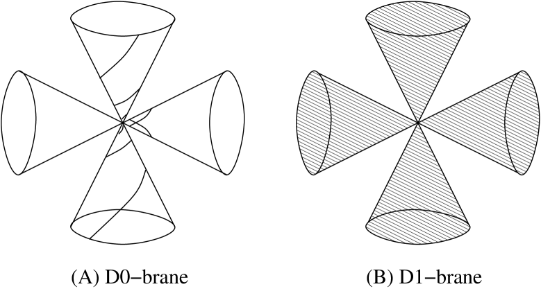
Figure 2: (A) D0-brane propagates from past infinity to future infinity by passing a whisker region. (B) D1-brane wraps the whole space-time and it may include gauge flux on it.

D-branes in Misner space may be obtained by utilizing orbifold method. In $\mathbb{R}^{1,1}$ we have D0-brane passing from infinite past to infinite future, and D1-brane with non-trivial gauge flux on its worldvolume. The trajectory of a particle (D0-brane in our case) in Misner space is given in [64] as follows. It starts from far past in the cosmological region $t\sim-\infty$ and approaches spirally into the big crunch singularity. Then it crosses a whisker region and goes to the other cosmological region (see figure 2). For D1-brane, we can construct only brane wraping the whole space-time. The gauge flux on it is obtained by minimizing the DBI action. In the cosmological regions we have

$$S=-\tau_{1}\int dtd\psi\sqrt{t^{2}-F_{t\psi}^{2}}.$$ (A.3)

Thus the gauge flux can be computed from the Gauss constraint

$$\frac{\delta{\cal L}}{\delta F_{t\psi}} =\frac{\tau_{1}F_{t\psi}}{\sqrt{t^{2}-F_{t\psi}^{2}}}=\Pi, F_{t\psi}^{2} =\frac{t^{2}}{1+\frac{\tau_{1}^{2}}{\Pi^{2}}}.$$ (A.4)

In the whisker regions, similar analysis leads to the gauge field

$$F_{r\tau}^{2}=\frac{r^{2}}{1+\frac{\tau_{1}^{2}}{\Pi^{2}}}.$$ (A.5)

We hope to present a more detailed report on the analysis of the D-branes including the boundary states for them in near future [60].

References

• [1] J. Khoury, B. A. Ovrut, N. Seiberg, P. J. Steinhardt and N. Turok, “From big crunch to big bang,” Phys. Rev. D 65, 086007 (2002) [arXiv:hep-th/0108187].
• [2] N. Seiberg, “From big crunch to big bang - is it possible?,” arXiv:hep-th/0201039.
• [3] V. Balasubramanian, S. F. Hassan, E. Keski-Vakkuri and A. Naqvi, “A space-time orbifold: A toy model for a cosmological singularity,” Phys. Rev. D 67, 026003 (2003) [arXiv:hep-th/0202187].
• [4] L. Cornalba, and M.  S.  Costa, “A New Cosmological Scenario In String theory,” Phys.  Rev.  D 66 066001 (2002) [arXiv:hep-th/0203031].
• [5] N. A. Nekrasov, “Milne universe, tachyons, and quantum group,” Surveys High Energ. Phys.  17, 115 (2002) [arXiv:hep-th/0203112].
• [6] J. Simon, “The geometry of null rotation identifications,” JHEP 0206, 001 (2002) [arXiv:hep-th/0203201].
• [7] H. Liu, G. W. Moore and N. Seiberg, “Strings in a time-dependent orbifold,” JHEP 0206, 045 (2002) [arXiv:hep-th/0204168].
• [8] L. Cornalba, M. S. Costa and C. Kounnas, “A resolution of the cosmological singularity with orientifolds,” Nucl. Phys. B 637, 378 (2002) [arXiv:hep-th/0204261].
• [9] A. Lawrence, “On the instability of 3D null singularities,” JHEP 0211, 019 (2002) [arXiv:hep-th/0205288].
• [10] H. Liu, G. W. Moore and N. Seiberg, “Strings in time-dependent orbifolds,” JHEP 0210, 031 (2002) [arXiv:hep-th/0206182].
• [11] M. Fabinger and J. McGreevy, “On smooth time-dependent orbifolds and null singularities,” JHEP 0306, 042 (2003) [arXiv:hep-th/0206196].
• [12] G. T. Horowitz and J. Polchinski, “Instability of space-like and null orbifold singularities,” Phys. Rev. D 66, 103512 (2002) [arXiv:hep-th/0206228].
• [13] M. Berkooz, B. Craps, D. Kutasov and G. Rajesh, “Comments on cosmological singularities in string theory,” JHEP 0303, 031 (2003) [arXiv:hep-th/0212215].
• [14] C. R. Nappi and E. Witten, “A closed, expanding universe in string theory,” Phys. Lett. B 293, 309 (1992) [arXiv:hep-th/9206078].
• [15] S. Elitzur, A. Giveon, D. Kutasov and E. Rabinovici, “From big bang to big crunch and beyond,” JHEP 0206 (2002) 017 [arXiv:hep-th/0204189].
• [16] P. Horava, “Some exact solutions of string theory in four-dimensions and five-dimensions,” Phys. Lett. B 278, 101 (1992) [arXiv:hep-th/9110067].
• [17] C. Kounnas and D. Lust, “Cosmological string backgrounds from gauged WZW models,” Phys. Lett. B 289, 56 (1992) [arXiv:hep-th/9205046].
• [18] B. Craps, D. Kutasov and G. Rajesh, “String propagation in the presence of cosmological singularities,” JHEP 0206, 053 (2002) [arXiv:hep-th/0205101].
• [19] Y. Hikida and T. Takayanagi, “On solvable time-dependent model and rolling closed string tachyon,” Phys. Rev. D 70, 126013 (2004) [arXiv:hep-th/0408124].
• [20] N. Toumbas and J. Troost, “A time-dependent brane in a cosmological background,” JHEP 0411, 032 (2004) [arXiv:hep-th/0410007].
• [21] N. Drukker, B. Fiol and J. Simon, “Gödel’s universe in a supertube shroud,” Phys. Rev. Lett.  91, 231601 (2003) [arXiv:hep-th/0306057].
• [22] J. P. Gauntlett, J. B. Gutowski, C. M. Hull, S. Pakis and H. S. Reall, “All supersymmetric solutions of minimal supergravity in five dimensions,” Class. Quant. Grav.  20, 4587 (2003) [arXiv:hep-th/0209114].
• [23] E. K. Boyda, S. Ganguli, P. Horava and U. Varadarajan, “Holographic protection of chronology in universes of the Gödel type,” Phys. Rev. D 67, 106003 (2003) [arXiv:hep-th/0212087].
• [24] T. Harmark and T. Takayanagi, “Supersymmetric Gödel universes in string theory,” Nucl. Phys. B 662, 3 (2003) [arXiv:hep-th/0301206].
• [25] Y. Hikida and S.-J. Rey, “Can branes travel beyond CTC horizon in Gödel universe?,” Nucl. Phys. B 669, 57 (2003) [arXiv:hep-th/0306148].
• [26] D. Brecher, P. A. DeBoer, D. C. Page and M. Rozali, “Closed timelike curves and holography in compact plane waves,” JHEP 0310, 031 (2003) [arXiv:hep-th/0306190].
• [27] D. Brace, C. A. R. Herdeiro and S. Hirano, “Classical and quantum strings in compactified pp-waves and Gödel type universes,” Phys. Rev. D 69, 066010 (2004) [arXiv:hep-th/0307265].
• [28] H. Takayanagi, “Boundary states for supertubes in flat space-time and Gödel universe,” JHEP 0312, 011 (2003) [arXiv:hep-th/0309135].
• [29] G. Sarkissian, “On D-branes in the Nappi-Witten and GMM models,” JHEP 0301, 059 (2003) [arXiv:hep-th/0211163].
• [30] T. Quella and V. Schomerus, “Asymmetric cosets,” JHEP 0302, 030 (2003) [arXiv:hep-th/0212119].
• [31] N. Seiberg and E. Witten, “String theory and noncommutative geometry,” JHEP 9909, 032 (1999) [arXiv:hep-th/9908142].
• [32] I. Bars and K. Sfetsos, “$SL(2,\mathbb{R})\times SU(2)/\mathbb{R}^{2}$ string model in curved space-time and exact conformal results,” Phys. Lett. B 301, 183 (1993) [arXiv:hep-th/9208001].
• [33] C. V. Johnson and H. G. Svendsen, “An exact string theory model of closed time-like curves and cosmological singularities,” Phys. Rev. D 70, 126011 (2004) [arXiv:hep-th/0405141].
• [34] E. Witten, “On string theory and black holes,” Phys. Rev. D 44, 314 (1991).
• [35] R. Dijkgraaf, H. Verlinde and E. Verlinde, “String propagation in a black hole geometry,” Nucl. Phys. B 371, 269 (1992).
• [36] M. Kato and T. Okada, “D-branes on group manifolds,” Nucl. Phys. B 499, 583 (1997) [arXiv:hep-th/9612148].
• [37] A. Y. Alekseev and V. Schomerus, “D-branes in the WZW model,” Phys. Rev. D 60, 061901 (1999) [arXiv:hep-th/9812193].
• [38] L. Birke, J. Fuchs and C. Schweigert, “Symmetry breaking boundary conditions and WZW orbifolds,” Adv. Theor. Math. Phys.  3, 671 (1999) [arXiv:hep-th/9905038].
• [39] R. E. Behrend, P. A. Pearce, V. B. Petkova and J. B. Zuber, “Boundary conditions in rational conformal field theories,” Nucl. Phys. B 570, 525 (2000) [Nucl. Phys. B 579, 707 (2000)] [arXiv:hep-th/9908036].
• [40] G. Felder, J. Frohlich, J. Fuchs and C. Schweigert, “The geometry of WZW branes,” J. Geom. Phys.  34, 162 (2000) [arXiv:hep-th/9909030].
• [41] J. M. Maldacena, G. W. Moore and N. Seiberg, “Geometrical interpretation of D-branes in gauged WZW models,” JHEP 0107, 046 (2001) [arXiv:hep-th/0105038].
• [42] K. Gawedzki, “Boundary WZW, G/H, G/G and CS theories,” Annales Henri Poincare 3, 847 (2002) [arXiv:hep-th/0108044].
• [43] S. Elitzur and G. Sarkissian, “D-branes on a gauged WZW model,” Nucl. Phys. B 625, 166 (2002) [arXiv:hep-th/0108142].
• [44] S. Fredenhagen and V. Schomerus, “D-branes in coset models,” JHEP 0202, 005 (2002) [arXiv:hep-th/0111189].
• [45] H. Ishikawa, “Boundary states in coset conformal field theories,” Nucl. Phys. B 629, 209 (2002) [arXiv:hep-th/0111230].
• [46] M. A. Walton and J. G. Zhou, “D-branes in asymmetrically gauged WZW models and axial-vector duality,” Nucl. Phys. B 648, 523 (2003) [arXiv:hep-th/0205161].
• [47] C. Bachas and M. Petropoulos, “Anti-de-Sitter D-branes,” JHEP 0102, 025 (2001) [arXiv:hep-th/0012234].
• [48] K. P. Yogendran, “D-branes in 2D Lorentzian black hole,” JHEP 0501, 036 (2005) [arXiv:hep-th/0408114].
• [49] C. Bachas and M. Porrati, “Pair creation of open strings in an electric field,” Phys. Lett. B 296, 77 (1992) [arXiv:hep-th/9209032].
• [50] K. Gödel, “An example of a new type of cosmological solutions of Einstein’s field equations of graviation,” Rev. Mod. Phys.  21, 447 (1949).
• [51] Y. Hikida, “String theory on Lorentzian $AdS_{3}$ in minisuperspace,” JHEP 0404, 025 (2004) [arXiv:hep-th/0403081].
• [52] B. Ponsot, V. Schomerus and J. Teschner, “Branes in the Euclidean $AdS_{3}$,” JHEP 0202, 016 (2002) [arXiv:hep-th/0112198].
• [53] S. Ribault and V. Schomerus, “Branes in the 2D black hole,” JHEP 0402, 019 (2004) [arXiv:hep-th/0310024].
• [54] N. Birrel and P. Davis, “Quantum fields in curved space,” Cambridge University Press (1984).
• [55] A. Strominger, “Open string creation by S-branes,” arXiv:hep-th/0209090.
• [56] M. Gutperle and A. Strominger, “Timelike boundary Liouville theory,” Phys. Rev. D 67, 126002 (2003) [arXiv:hep-th/0301038].
• [57] M. Berkooz, B. Pioline and M. Rozali, “Closed strings in Misner space: Cosmological production of winding strings,” JCAP 0408, 004 (2004) [arXiv:hep-th/0405126].
• [58] M. Berkooz, B. Durin, B. Pioline and D. Reichmann, “Closed strings in Misner space: Stringy fuzziness with a twist,” JCAP 0410, 002 (2004) [arXiv:hep-th/0407216].
• [59] D. Israël, “D-branes in Lorentzian $AdS_{3}$,” arXiv:hep-th/0502159.
• [60] Work in progress.
• [61] C. W. Misner, “Taub-NUT space as a counterexample to almost anything,” Relativity Theory and Astrophysics I: Relativity and Cosmology, ed. J. Ehlers, Lectures in Applied Mathematics, Volume 8, American Mathematical Society, 160 (1967).
• [62] S. W. Hawking and G. F. R. Ellis, “The large scale structure of space-time,” Cambrige University Press (1973).
• [63] M. Berkooz and B. Pioline, “Strings in an electric field, and the Milne universe,” JCAP 0311, 007 (2003) [arXiv:hep-th/0307280].
• [64] B. Durin and B. Pioline, “Closed strings in Misner space: A toy model for a big bounce?,” arXiv:hep-th/0501145.