Non perturbative regularization of one–loop integrals at finite temperature

Abstract

A method devised by the author is used to calculate analytical expressions for one–loop integrals at finite temperature. A non-perturbative regularization of the integrals is performed, yielding expressions of non-polynomial nature. A comparison with previously published results is presented and the advantages of the present technique are discussed.

I Introduction

In this paper we present a new technique which allows to evaluate non-perturbatively one–loop integrals occurring in finite temperature problems in quantum field theory. Such integrals typically involve series, due to summation over the the Matsubara frequencies, $\omega_{n}=2\pi nT$, with $n=0,\pm 1,\dots$ FW71 , which cannot be done analytically.

The method that we propose here is derived from the powerful ideas of the Linear Delta Expansion (LDE) and of Variational Perturbation Theory (VPT) (see LDEVPT and references therein); we briefly sketch how such methods work.

First one interpolates a non-perturbative lagrangian (hamiltonian) ${\cal L}$ with a solvable one ${\cal L}_{0}$, which depends on one or more arbitrary parameters; the interpolated lagragian is then split into a “leading” term, chosen to be ${\cal L}_{0}$ itself and into a “perturbation”, ${\cal L}-{\cal L}_{0}$. Although the “perturbative” term will not be a-priori small, a perturbative expansion is carried out and physical quantities are calculated. To finite order in perturbation theory one thus obtains expression which contain an artificial dependence upon the arbitrary parameters: however if the expansion were to be carried out to all orders such dependence would have to cancel out provided that the perturbative series converges. In order to minimize such dependence one applies the Principle of Minimal Sensitivity (PMS) Ste81 , which selects the value of the arbitrary parameter for which the physical quantity is less sensitive to changes in the parameter itself. The parameter determined in this way is normally such to make ${\cal L}-{\cal L}_{0}$ a perturbation and depends on the “natural” parameters present in ${\cal L}$. For this reason, the expansion obtained by using this method does not provide, to a finite order, a polynomial in the parameters of the model, as would be the case for a genuinely perturbative technique.

The ideas behind the LDE and the VPT are really very general and have been successful in dealing with a variety of problems of quite different nature, ranging from quantum field theory to classical and quantum mechanics. In this paper, in particular, we pursue the application of some results which were recently obtained by the author Am_zeta04 : in that paper the author developed a method to accelerate the convergence of certain class of mathematical series (including the Riemann and Hurwitz zeta functions) and proved that the new series obtained in such a way converge exponentially to the correct results. As we will see in this paper, some of the series treated in Am_zeta04 are relevant for the evaluation of one–loop integrals at finite temperature and will be used to obtain arbitrarily precise analytical approximations to such integrals which are not polynomials in the inverse temperature.

The paper is organized as follows: in section II we review some of the results of Am_zeta04 and explain the method; in section III we apply the results of section II to the calculation of one–loop integrals at finite temperature and compare them with the results in the literature DJ74 ; LV97 ; AE93 ; HW82 ; finally in section IV we draw our conclusions and discuss further possible applications of this method.

II The method

In this section we describe the method of Am_zeta04 , which allows one to accelerate the convergence of certain series. One of the applications which was discussed in that paper is to the zeta-like function defined as

$$\zeta(u,s,\xi)\equiv\sum_{n=0}^{\infty}\frac{1}{(n^{u}+\xi)^{s}}\ ,$$ (1)

where $s$, $u$ and $\xi$ are real parameters. The special cases obtained by taking $(u,\xi)=(1,1)$ or $u=1$ correspond to the Riemann and Hurwitz zeta functions respectively. Further examples of application of this method are contained in Am_zeta04 and the interested reader should refer to that paper for further reading.

We write

$$\zeta(u,s,\xi) = \frac{1}{\xi^{s}}+\sum_{n=1}^{\infty}\frac{1}{\left(n^{u}+\xi\right)^{s}}$$ (2)

and by simple algebra we convert it to the form

$$\zeta(u,s,\xi) = \frac{1}{\xi^{s}}+\sum_{n=1}^{\infty}\frac{1}{n^{su}}\ \frac{1}{\left(1+\lambda^{2}\right)^{s}}\frac{1}{\left(1+\Delta(n)\right)^{s}}$$ (3)

having introduced the definition

$$\Delta(n) \equiv \frac{\xi/n^{u}-\lambda^{2}}{1+\lambda^{2}}\ .$$ (4)

We stress that eq. (3) is still an identity and that no approximation has been made so far. $\lambda$ here is an arbitrary parameter which was introduced “ad hoc”: this procedure is typical of the Linear Delta Expansion (LDE) and of Variational Perturbation Technique (VPT) LDEVPT .

Clearly, when the condition $|\Delta(n)|<1$ is met, one can expand eq. (3) in powers of $\Delta$; such a condition requires that $\left|\frac{\xi-\lambda^{2}}{1+\lambda^{2}}\right|<1$, i.e. that $\lambda^{2}>\frac{\xi-1}{2}$.

We can therefore write

$$\frac{1}{(1+\Delta(n))^{s}}=\sum_{k=0}^{\infty}\frac{\Gamma(k+s)}{\Gamma(s)\ k!}\ (-\Delta(n))^{k}$$ (5)

and convert the series (3) to the equivalent series:

$$\zeta(u,s,\xi) = \frac{1}{\xi^{s}}+\sum_{n=1}^{\infty}\sum_{k=0}^{\infty}\frac{\Gamma(k+s)}{\Gamma(s)\ k!}\ \sum_{j=0}^{k}\ \left(\begin{array}[]{c}k\\ j\\ \end{array}\right)\frac{\lambda^{2(k-j)}}{(1+\lambda^{2})^{s+k}}\frac{(-\xi)^{j}}{n^{u(s+j)}}\ .$$ (8)

By interchanging the sums and performing the sum over $n$ we finally obtain the expression

$$\zeta(u,s,\xi) = \frac{1}{\xi^{s}}+\sum_{k=0}^{\infty}\frac{\Gamma(k+s)}{\Gamma(s)}\ \sum_{j=0}^{k}\ \frac{(-\xi)^{j}}{j!(k-j)!}\frac{\lambda^{2(k-j)}}{(1+\lambda^{2})^{s+k}}\zeta(u(s+j))\ .$$ (9)

We stress that eq. (9) is still exact for $\lambda^{2}>\frac{\xi-1}{2}$ and that it converges exponentially. Actually this equation describes an entire family of series, all converging to the same function, although with different rates of convergence. When the sum in eq. (9) is truncated to a finite value, a fictitious dependence on the arbitrary parameter $\lambda$ is generated: in order to minimize such dependence and to obtain a series with an optimal rate of convergence one can apply the Principle of Minimal Sensitivity (PMS) Ste81 , corresponding to selecting the value of $\lambda$ for which the derivative of the partial sum with respect to $\lambda$ vanishes.

To leading order one obtains the result

$$\lambda_{PMS}^{(1)} = \sqrt{\xi}\ \sqrt{\frac{\zeta(u(1+s))}{\zeta(su)}},$$ (10)

which can then be used inside eq. (9). The precision of these formulas has been investigated in Am_zeta04 , showing that extremely precise results are in general obtained already working to low orders.

III Applications: one–loop integrals at finite temperature

We will follow the notation set in LV97 and write the expression for a general one–loop integral at finite temperature in the form

$$J(m,a,b) = T\mu^{2\epsilon}\sum_{\begin{array}[]{c}n=-\infty\\ n\neq 0\\ \end{array}}^{\infty}\int\frac{d^{D}k}{(2\pi)^{D}}\ \frac{(k^{2})^{a}}{\left[k^{2}+\omega_{n}^{2}+m^{2}\right]^{b}}$$ (13)

$\mu$ being the scale brought in by dimensional regularization, $a$ and $b$ being integers ($a\geq 0$ and $b>0$). Following LV97 we also define

$$K^{2}\equiv\left(\frac{k}{2\pi T}\right)^{2}\ ,\ \ M^{2}\equiv\left(\frac{m}{2\pi T}\right)^{2}\ ,\ \ \Omega^{2}\equiv\left(\frac{\mu}{2\pi T}\right)^{2}$$

and obtain

$$J(M,a,b) = T\ \left(2\pi T\right)^{3+2a-2b}\ 2\Omega^{2\epsilon}$$ (14)

$$\cdot \frac{\pi^{D/2}}{(2\pi)^{D}}\ \frac{\Gamma(D/2+a)}{\Gamma(D/2)}\ \frac{\Gamma(l)}{\Gamma(b)}\ S(M,l)$$

where

$$S(M,l) = \sum_{n=1}^{\infty}\ \frac{1}{(n^{2}+M^{2})^{l}}$$ (15)

and $l=b-a-D/2$ and $D=3-2\ \epsilon$. Depending upon the value of $l$, the series of eq. (15) could be divergent and therefore need regularization.

Eq. (15) is clearly of the form considered in eq. (1) and one can write

$$S(M,l) = -\frac{1}{M^{2l}}+\zeta(2,l,M^{2})\ ,$$ (16)

where

$$\zeta(2,l,M^{2}) = \frac{1}{M^{2l}}$$ (17)

$$+ \sum_{k=0}^{\infty}\frac{\Gamma(k+l)}{\Gamma(l)}\ \Psi_{k}(\lambda,2,l,M^{2})$$

and

$$\Psi_{k}(\lambda,2,l,M^{2}) \equiv \frac{1}{(1+\lambda^{2})^{s+k}}$$

$$\cdot \sum_{j=0}^{k}\ \frac{(-M^{2})^{j}}{j!(k-j)!}\lambda^{2(k-j)}\zeta(2(l+j))\ .$$

Once more we stress that although the series all converge to the same result independently of $\lambda$ (provided that $\lambda>\frac{\xi-1}{2}$), the partial sums, obtained by truncating the series to a finite order will necessarily display a dependence on the parameter. Such dependence, which is an artifact of working to a finite order, will also make the rate of convergence of the different elements of the family $\lambda$-dependent. Since it is desirable to obtain the most precise results with the least effort, one will select the optimally convergent series by fixing $\lambda$ through the “principle of minimal sensitivity” (PMS) Ste81 . The solutions obtained by applying this simple criterion display in general the highest convergence rate and, once plugged back in the original series, provide a non-polynomial expression in the natural parameters.

In the present case, the “natural” parameter in eq. (15) is $M^{2}$ and to first–order the PMS yields

$$\lambda_{PMS}^{(1)} = \sqrt{M^{2}}\ \sqrt{\frac{\zeta(2(1+l))}{\zeta(2l)}},$$ (18)

On the other hand, if the value $\lambda=0$ is chosen, then one obtains the series

$$\zeta(2,l,M^{2}) = \frac{1}{M^{2l}}$$ (19)

$$+ \sum_{k=0}^{\infty}\frac{\Gamma(k+l)}{\Gamma(l)}\ \frac{(-M^{2})^{k}}{k!}\ \zeta(2(l+k))\ ,$$

which, to a finite order yields a polynomial in $M$. Notice that such series corresponds to the expansion used in LV97 .

In fig. 1 we have compared $\zeta(2,3/2,\xi)$ calculated numerically with the first–order approximations obtained by using eq. (17) with $\lambda=\lambda_{PMS}^{(1)}$ and $\lambda=0$, which are

$$\zeta_{PMS}^{(1)}(2,3/2,\xi) = \frac{1}{\xi^{3/2}}+\frac{\zeta(3)^{5/2}}{{\left(\zeta(3)+\xi\,\zeta(5)\right)}^{3/2}}$$ (20)

$$\zeta_{\lambda=0}^{(1)}(2,3/2,\xi) = \frac{1}{\xi^{3/2}}+\zeta(3)-\frac{3}{2}\,\xi\,\zeta(5)\ ,$$ (21)

where the second and third term in the second equation can be obtained by Taylor expanding the first equation.

In table 1 we have calculated $\zeta(2,3/2,1)$ using eq. (17) to order $N$ with $\lambda_{PMS}^{(1)}$ (second column) and with $\lambda=0$ (third column). Our formula, using the optimal parameter obtained to first order, converges exponentially to the exact value, whereas the formula corresponding to $\lambda=0$ is actually useless (that formula is indeed limited to $\xi\ll 1$). Notice that $\zeta(2,3/2,1)$ calculated with the first $10^{5}$ terms in eq. (1) gives the result $\underline{1.5124349215}0$; the same precision is reached with our improved series with only $27$ terms. We believe that this result by itself is sufficient to illustrate the strength of our method.

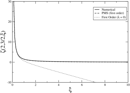
Figure 1: $\zeta(2,3/2,\xi)$ calculated numerically (solid line), with the PMS to first order (dashed line) and using $\lambda=0$ (dotted line).

Table 1: $\zeta(2,3/2,1)$ calculated using eq. (17) to order $N$ with $\lambda_{PMS}^{(1)}$ (second column) and with $\lambda=0$ (third column). The underlined digits are correct.

$N$	$\zeta_{PMS}(2,3/2,1)$	$\zeta_{\lambda=0}(2,3/2,1)$
1	1.4728636067646540152245808470808148333385501418201	0.64666527044453939590268993182589873867936491308763
10	1.5124141548516402130603869952574426525740627123155	3.4054827271508252417934796716746660253808017949304
100	1.5124349215502030648030954892350003557973564160761	7.189509053068942853725754726982871981048977697327
200	1.5124349215502030648030954892350003618366746247481	9.5161848472956355375285584079161971312864869056589

As an example of the application of our formula, we consider the case studied in eq. (12) of LV97 , i.e.

$$I(m) = T\ \mu^{2\epsilon}\ \sum_{n=-\infty}^{+\infty}\int\frac{d^{D}k}{(2\pi)^{D}}\ \frac{1}{k^{2}+M^{2}}$$ (22)

$$= T\ \mu^{2\epsilon}\ \int\frac{d^{D}k}{(2\pi)^{D}}\ \frac{1}{k^{2}+M^{2}}+J(M,0,1)$$

which is essentially the one-loop self energy.

The first integral is finite and equal to $-MT/(4\pi)$ whereas the second term can be written as:

$$J(M,0,1) = 2^{-2-2\epsilon}\ \pi^{-3/2-3\epsilon}\ \mu^{2\epsilon}\ T^{1-4\epsilon}\ \Gamma(-1/2+\epsilon)\ \left[-\frac{1}{M^{-1-2\epsilon}}+\zeta(2,-1/2+\epsilon,M^{2})\right]\ ,$$ (23)

where the divergencies are contained in $\zeta(2,-1/2+\epsilon,M^{2})$.

By using our eq. (19) and retaining only the divergent terms and those independent of $\epsilon$ we obtain

$$I(m) = -\frac{mT}{4\pi}+\frac{T^{2}}{12}-\frac{m^{2}}{16\pi^{2}}\ \left[\frac{1}{\epsilon}+\gamma-\log\frac{4\pi T^{2}}{\mu^{2}}\right]$$ (24)

$$+ \frac{m^{4}\zeta(3)}{8(2\pi)^{4}T^{2}}-\frac{m^{6}\,\zeta(5)}{1024\,{\pi}^{6}\,T^{4}}+\frac{5\,m^{8}\,\zeta(7)}{32768\,{\pi}^{8}\,T^{6}}$$

$$- \frac{7\,m^{10}\,\zeta(9)}{262144\,{\pi}^{10}\,T^{8}}+\dots$$

which reproduces the results of LV97 , which, however, were considered only up to order $m^{4}$. As anticipated, the formula obtained is a polynomial in $m$.

We will now use the optimal series (17) to improve this result. We first notice that since

$$\frac{d\zeta(u,s,\xi)}{d\xi} = -s\ \zeta(u,s+1,\xi)$$ (25)

a divergent series can be related to a convergent series by taking repeated derivatives with respect to the parameter $\xi$. Indeed by applying eq. (25) twice we can write the general expression

$$J(M,a,b) = \frac{2^{1+2\,a-2\,b+2\,{\epsilon}}\,{{\Omega}}^{2\,{\epsilon}}\,{\pi}^{\frac{3}{2}+2\,a-2\,b+{\epsilon}}\,T^{4+2\,a-2\,b}\,\Gamma(\frac{3}{2}+a-{\epsilon})\,\Gamma(-\left(\frac{3}{2}\right)-a+b+{\epsilon})}{\Gamma(b)\,\Gamma(\frac{3}{2}-{\epsilon})}$$ (26)

$$\cdot \left(1+a-b+\frac{3-2\,{\epsilon}}{2}\right)\,\left(-a+b+\frac{-3+2\,{\epsilon}}{2}\right)$$

$$\cdot \left\{\int dM^{2}\int dM^{2}\left(-M^{-2\,\left(2-a+b+\frac{-3+2\,{\epsilon}}{2}\ \right)}+\zeta(2,\frac{1}{2}-a+b+\epsilon,M^{2})\right)\right\}$$

where the last $\zeta$ function is now fully convergent when $a=0$ and $b=1$. Since this formula requires a double integration of a convergent series, the result is determined up to two constants of integration, which will contain the divergent contributions.

By applying eq. (17) to first order and using the optimal value of $\lambda$ given by eq. (18) we obtain the simple result

$$J_{PMS}(M,0,1) = T^{2}\ \left(-\kappa_{1}\ M^{2}-\frac{{\zeta(3)}^{5/2}\ {\sqrt{\zeta(3)+M^{2}\,\zeta(5)}}}{{\zeta(5)}^{2}}\right)+\kappa_{2}$$

where $\kappa_{1,2}$ are the constants of integration independent of $M$. In order to determine these constants we Taylor expand this expression in $M$ and then use $M=m/(2\pi T)$ thus obtaining

$$J(M,0,1) \approx \kappa_{2}-\frac{\left(\kappa_{1}\,m^{2}\right)}{4\,{\pi}^{2}}+\frac{m^{4}\,\zeta(3)}{128\,{\pi}^{4}\,T^{2}}-\frac{T^{2}\,{\zeta(3)}^{3}}{{\zeta(5)}^{2}}$$ (28)

$$- \frac{m^{2}\,{\zeta(3)}^{2}}{8\,{\pi}^{2}\,\zeta(5)}-\frac{m^{6}\,\zeta(5)}{1024\,{\pi}^{6}\,T^{4}}+\frac{5\,m^{8}\,{\zeta(5)}^{2}}{32768\,{\pi}^{8}\,T^{6}\,\zeta(3)}$$

$$- \frac{7\,m^{10}\,{\zeta(5)}^{3}}{262144\,{\pi}^{10}\,T^{8}\,{\zeta(3)}^{2}}+\dots$$

This expression can be now compared with the perturbative result and the constants of integration can thus be extracted

$$\kappa_{1} = \frac{1}{4}\left[\frac{1}{\epsilon}+\gamma-\log\left(\frac{4\pi T^{2}}{\mu^{2}}\right)-\frac{2\,{{\zeta}(3)}^{2}}{{\zeta}(5)}\right]$$

$$\kappa_{2} = \frac{1}{12}+\frac{{{\zeta}(3)}^{3}}{{{\zeta}(5)}^{2}}\ .$$

Eq. (LABEL:jpms0) is a quite remarkable formula: indeed, although it has been derived by applying our method to first order, it reproduces correctly the terms going as $m^{4}$ and $m^{6}$ and it also provides the coefficients of the higher order terms apart from factors depending on the Riemann $\zeta$ function evaluated at odd integer values . Of course, we can let the perturbative result guide us further and use the fact that $\lim\limits_{n\rightarrow\infty}\zeta(n)=1$ to write the improved formula

$$J_{PMS2}(M,0,1) = \frac{13}{12}\ T^{2}-\frac{M^{2}\,T^{2}}{4}\ \left[\frac{1}{\epsilon}+\gamma-\log\left(\frac{4\pi T^{2}}{\mu^{2}}\right)-2\right]$$ (29)

$$- \frac{T^{2}}{16}\ \left[\left(16\,{\sqrt{1+M^{2}}}-2\,M^{4}\,\left(-1+\zeta(3)\right)+M^{6}\,\left(-1+\zeta(5)\right)\right)\right]\ ,$$

where the notation $PMS2$ has been introduced to distiguish it from the previous formula. Notice that both equations (LABEL:jpms0) and (29) are non–polynomial in $m$.

By putting the pieces together we finally obtain our approximation to $I(m)$, given by

$$I_{PMS2}(M) = -\frac{MT^{2}}{2}+\frac{13}{12}\ T^{2}-\frac{M^{2}\,T^{2}}{4}\ \left[\frac{1}{\epsilon}+\gamma-\log\left(\frac{4\pi T^{2}}{\mu^{2}}\right)-2\right]$$ (30)

$$- \frac{T^{2}}{16}\ \left[\left(16\,{\sqrt{1+M^{2}}}-2\,M^{4}\,\left(-1+\zeta(3)\right)+M^{6}\,\left(-1+\zeta(5)\right)\right)\right]\ .$$

When negative values of $m^{2}$ are considered, corresponding to a spontaneously broken phase, these results hold for $T\geq T_{0}\equiv-m^{2}/(4\pi^{2})$.

As a further application of the method described in this paper we consider the integral

$${\cal J}(\phi)=\frac{T}{2}\mu^{-2\epsilon}\sum_{k_{0}}\int\frac{d^{3-2\epsilon}k}{(2\pi)^{3-2\epsilon}}\ \log\left(k^{2}+m^{2}(\phi)\right)$$ (31)

where $k_{0}=2\pi nT$, for all $n$ integers. The effective potential to one–loop is expressed in terms of this integral.

Given the relation

$$I(m) = \frac{1}{m}\ \frac{d{\cal J}}{dm}$$ (32)

it is not necessary to calculate ${\cal J}(m)$ which can be obtained as

$${\cal J}(m)=\int I(m)\ m\ dm+\rho\ ,$$ (33)

where $\rho$ is constant of integration independent of $m$.

By using $I_{PMS2}$ of eq. (30) we obtain the simple expression:

$${\cal J}_{PMS2}(m) = \rho+\frac{13}{24}\,m^{2}\,T^{2}-\frac{m^{3}\,T}{12\,\pi}$$ (34)

$$- \frac{T}{6\pi}\ \left(m^{2}+4\ \pi^{2}T^{2}\right)^{3/2}$$

$$- \frac{m^{4}}{64\pi^{2}}\ \left[\frac{1}{\epsilon}+\gamma-\log\left(\frac{4\pi T^{2}}{\mu^{2}}\right)-2\right]$$

$$+ \frac{m^{6}}{768\ \pi^{4}T^{2}}\ \left(\zeta(3)-1\right)$$

$$- \frac{m^{8}}{8192\ \pi^{6}T^{4}}\ \left(\zeta(5)-1\right)$$

which can be expanded in powers of $m$ to give

$${\cal J}_{PMS2}(m) = \rho-\frac{4\,{\pi}^{2}\,T^{4}}{3}+\frac{m^{2}\,T^{2}}{24}-\frac{m^{3}\,T}{12\,\pi}$$ (35)

$$- \frac{m^{4}}{64\pi^{2}}\,\left(\frac{1}{\epsilon}+\gamma-\log\left(\frac{4\pi T^{2}}{\mu^{2}}\right)\right)$$

$$+ \frac{m^{6}\zeta(3)}{768\,{\pi}^{4}\,T^{2}}-\frac{m^{8}\zeta(5)}{8192\,{\pi}^{6}\,T^{4}}$$

$$+ \frac{m^{10}}{65536\,{\pi}^{8}\,T^{6}}+\dots$$

which reproduces exactly eq. (3.7) of AE93 , provided that $\rho=\frac{4\pi^{2}T^{4}}{3}+constant$. This last constant is independent both of $m$ and of $T$.

We are now in a position to compare our result of eq. (34) with the high temperature expansion of eq.(42) of ref. HW82 which reads

$$\frac{\Omega}{2VT^{4}} = -\frac{\pi^{2}}{90}+\frac{y^{2}}{6}-\frac{y^{3}}{12\pi}+\frac{y^{4}}{32\pi^{2}}\ \left[\log\frac{4\pi}{y}-\gamma+\frac{3}{4}\right]$$

$$- \frac{y^{4}}{16\pi^{2}}\sum_{k=1}^{\infty}(-1)^{k}\ \left(\frac{y}{4\pi}\right)^{k}\ \frac{\Gamma(2k+1)\ \zeta(2k+1)}{\Gamma(k+1)\ \Gamma(k+3)}$$

after setting the chemical potential to zero. We have defined $y=m/T$.

As we can see from table 2 the result of LV97 for $I(m)$ would essentially provide the expansion of eq. (LABEL:hw) and thus reproduce the results obtained long time ago by Haber and Weldon HW82 . We regard this procedure as “perturbative” meaning that, when the series in eq. (LABEL:hw) is truncated a polynomial in powers of $m/T$ is obtained. On the other hand, our simple formula, eq. (34) reproduces correctly the perturbative expansion of HW82 up to order $(m/T)^{8}$, and up to a factor involving the $\zeta$ function calculated at odd integer values, which however tend to $1$ for large values. This makes our simple formula quite precise. We remind the reader that eq. (34) was obtained by applying our method to first order and that, given the convergence of the method, drastic improvements in the quality of the approximation are expected if higher orders would to be taken into account. Although the calculation of higher orders with our method would be an interesting issue by itself, we will leave it for future work.

In fig. 2 we have plotted $\tilde{{\cal J}}_{PMS2}/T^{4}$, defined by taking out the terms up to order $(m/T)^{4}$, and the similar functions obtained from eq. (LABEL:hw), performing the sum to three different orders ($k_{max}=10,20,30$). The horizontal scale is $y=m/T$. We leave to the reader any judgement on the quality of our approximation. Notice that the series of Haber and Weldon should correspond to our variational series for $\lambda=0$; as we have seen before the criterion of convergence for a series is that $\lambda^{2}>\frac{M^{2}-1}{2}$, which for $\lambda=0$ can be fullfilled only if $m/T<2\pi$. Looking at the figure we indeed see that when we get close to this value the sum of HW82 becomes ill–behaved.

Table 2: Comparison between eq. (LABEL:hw) and the simple approximation of eq. (34).

$N$	eq. (LABEL:hw)	${\cal J}_{PMS2}/T^{4}$
$\left[\frac{m}{T}\right]^{6}$	$\frac{\zeta(3)}{768\ \pi^{4}}$	$\frac{\zeta(3)}{768\,\pi^{4}}$
$\left[\frac{m}{T}\right]^{8}$	$-\frac{\zeta(5)}{8192\ \pi^{6}}$	$-\frac{\zeta(5)}{8192\ \pi^{6}}$
$\left[\frac{m}{T}\right]^{10}$	$\frac{\zeta(7)}{65536\ \pi^{8}}$	$\frac{1}{65536\ \pi^{8}}$
$\left[\frac{m}{T}\right]^{12}$	$-\frac{7\ \zeta(9)}{3145728\ \pi^{10}}$	$-\frac{7}{3145728\ \pi^{10}}$
$\left[\frac{m}{T}\right]^{14}$	$\frac{3\ \zeta(11)}{8388608\ \pi^{12}}$	$\frac{3}{8388608\ \pi^{12}}$

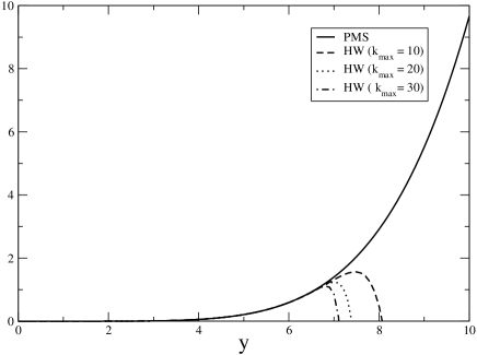
Figure 2: Comparison between $\tilde{{\cal J}}_{PMS2}/T^{4}$ and eq. (LABEL:hw) taking $k_{max}=10$ (dashed), $k_{max}=20$ (dotted) and $k_{max}=30$ (dot-dashed) terms.

IV Conclusions

The method that we have described in this paper is quite general and probably could be extended in the future to deal with a larger class of problems than the one presented here. We have proved that, by using variational techniques it is possible to estimate analytically and to an arbitrary degree of precision series which are difficult to evaluate with standard techniques. In particular, we have shown that by relating divergent series to convergent ones through repeated derivatives and then matching the divergences contained in the constants of integration with the ones coming out of the perturbative calculation, it is possible to construct a really non–perturbative regularization. Such regularized expressions are very accurate even at low orders and low temperatures. There is a huge literature dealing with field theoretical problems at finite temperature and we feel that this paper can provide a quite general and useful tool to attack many of these problems. We also believe, although at present is still to be confirmed, that the method that we have described could be useful in the non–perturbative calculation of the Casimir effect, for which zeta function regularization is a well–established technique (see for example Ez02 ). It would be quite interesting to see if non–perturbative expressions for the Casimir effect could be calculated analytically. We hope to apply these ideas to such a problem in the near future. As a final remark, we like to stress that despite the simplicity of the ideas that we have illustrated, all the results that we have obtained are fully analytical and improvable to the desired level of accuracy.

- (1) A.L. Fetter and J.D. Walecka, Quantum Theory of Many Particle Systems, McGraw-Hill, Boston,1971
- (2) A. Duncan and M. Moshe, Phys. Lett. B 215, 352 (1988); I.R.C. Buckley, A. Duncan and H.F. Jones, Phys.Rev.D47:2554-2559,1993; G. A. Arteca, F. M. Fernández, and E. A. Castro, Large order perturbation theory and summation methods in quantum mechanics (Springer, Berlin, Heidelberg, New York, London, Paris, Tokyo, Hong Kong, Barcelona, 1990); H. Kleinert, Path Integrals in Quantum Mechanics, Statistics and Polymer Physics, 3rd edition (World Scientific Publishing, 2004)
- (3) P. M. Stevenson, Phys. Rev. D 23, 2916 (1981)
- (4) P. Amore, ArXiv:[math-ph/0408036]
- (5) L. Dolan and R. Jackiw, Phys. Rev. D 9, 3320 (1974)
- (6) L. Vergara, Journal of Physics A 30, 6977 (1997)
- (7) P. Arnold and O. Espinosa, Phys. Rev. D 47, 3546 (1993)
- (8) H.E. Haber and H.A. Weldon, J. Math. Phys. 23, 1852 (1982)
- (9) G. Cognola, E. Elizalde and S. Zerbini, Phys. Rev. D 65, 085031 (2002)