FTI/UCM 70-2005

The $U(1)_{A}$ anomaly in noncommutative $SU(N)$ theories.

C.P. Martín and C. Tamarit Departamento de Física Teórica I, Facultad de Ciencias Físicas
Universidad Complutense de Madrid, 28040 Madrid, Spain

PACS: 11.15.-q; 11.30.Rd; 12.10.Dm
Keywords: $U(1)_{A}$ anomaly, Seiberg-Witten map, noncommutative gauge theories.

1 Introduction

Some of the peculiar and beautiful properties of QCD in the low-energy regime can be explained with the help of the famous $U(1)_{A}$ anomaly equation. A conspicuous instance of this state of affairs is the occurrence of the interaction through instantons between left-handed quarks and right-handed antiquarks; a phenomenon which is heralded by the existence of the $U(1)_{A}$ anomaly. That interaction process provided the solution given in ref. [1] to the so-called $U(1)_{A}$ problem. Other instances that show the importance of the $U(1)_{A}$ anomaly in particle physics can be found in ref. [2].

Many are the pitfalls that one meets when constructing noncommutative gauge theories [3, 4, 5, 6, 7]. In particular, it is not easy to build noncommutative field theories for $SU(N)$ gauge groups. Alas! The Moyal product of two local infinitesimal $SU(N)$ transformations is not a local infinitesimal $SU(N)$ transformation [8]. Further, charges different from $+1,0,-1$ do not fit in the standard noncommutative setup as developed for $U(N)$ groups [9, 10, 11]. These problems were addressed and given a solution in refs. [12, 13], where the appropriate framework was developed: the framework is based on the concept of Seiberg-Witten map. Both the noncommutative Standard Model [14] and the noncommutative generalizations [15, 16] of the ordinary $SU(5)$ and $SO(10)$ grand unified theories have been constructed within this framework. These noncommutative generalizations of ordinary theories are not renormalizable [17, 18], so that they must be formulated as effective quantum field theories. A nice feature of these theories is that their chiral matter content make them free from gauge anomalies [19, 20]. The study of the phenomenological consequences of the noncommutative Standard Model has just begun: see refs. [21, 22, 23]. The reader is further referred to refs. [24, 25] for other noncommutative models that generalize the ordinary standard model and are formulated within the standard noncommutative framework for $U(N)$ –not $SU(N)$– groups. Now a point of terminology: by noncommutative $SU(N)$ gauge theories we shall mean field theories constructed, for $SU(N)$ groups, within the framework in refs. [12, 13].

The $U(1)_{A}$ anomaly and its consequences have been intensively studied for nocommutative $U(N)$ theories within the standard noncommutative setup, i.e., the Seiberg-Witten map is not used to define the noncommutative fields. The reader is referred to refs. [26, 27, 28, 29, 30, 32, 33, 35] for further information. However, no such study has been carried out for noncommutative $SU(N)$ gauge theories as yet. The purpose of this paper is to remedy this situation and work out the anomaly equation for the $U(1)_{A}$ canonical Noether current up to second order in the noncommutative parameter $h$ –i.e., second order in $\theta^{\mu\nu}$– and at the one-loop level. This is a highly non-trivial issue since already at first order in $h$ there are candidates to the $U(1)_{A}$ anomaly whose Wick rotated space-time volume integral does not vanish for a general field configuration with non-vanishing Pontriagin index. An instance of such candidates reads

$$\theta^{\rho\sigma}\epsilon^{\mu_{1}\mu_{2}\mu_{3}\mu_{4}}\text{Tr}\,[f_{\sigma\mu_{1}}f_{\mu_{2}\mu_{3}}f_{\rho\mu_{4}}].$$

At second order in $h$ the situation worsens.

We shall also discuss the relationship, both at classical and quantum levels, between this canonical Noether current and other $U(1)_{A}$ currents that are the analogs of the $U(1)_{A}$ canonical Noether currents –see refs. [26, 27, 28, 29, 30]– that occur in noncommutative $U(N)$ gauge theories with fermions in the fundamental representation. These analogs, unlike the canonical Noether current of the noncommutative $SU(N)$ theory, are local $\star$-polynomials of the noncommutative fermion fields only. Barring a concrete instance, we shall not be able to give expressions for the $U(1)_{A}$ anomaly equation valid at any order in $h$ since the type of Feynman integrals to be computed depends on the order in $h$. This was not the case for chiral gauge anomalies –see ref. [20]–, since there the gauge current is of the planar kind and, thus, the one-loop Feynman integrals to be worked out are of the same type at any order in $h$. We shall show besides that the nonsinglet chiral currents are conserved at the one-loop level and, this time, at any order in $h$.

Our noncommutative $SU(N)$ theory will be massless and will have $N_{f}$ fermion flavours, all fermions carrying the same, but arbitrary, representation of $SU(N)$. The generalization of our expressions to more general situations is achieved by summing over all representations carried by the fermions in the theory. The layout of this paper is as follows. The first section is devoted to the study, at the classical level, of the chiral symmetries of the theory and the corresponding conservation equations. In this section, we introduce as well several currents that are either conserved or covariantly conserved as a consequence of the rigid $U(1)_{A}$ symmetry of the action. In section two, we compute the would-be anomalous contributions to the classical conservation equations of these currents. In the third section, we discuss the conservation of the nonsinglet currents at the one-loop level. Then, it comes the section which contains a summary of the results obtained in this paper and where our conclusions are stated. In this last section we also adapt our results to $SO(10)$ and $U(1)$ noncommutative gauge theories. Finally, we include several Appendices that the reader may find useful in reproducing the calculations presented in the sequel.

2 Classical chiral symmetries and currents

The classical action of the noncommutative $SU(N)$ gauge theory of a noncommutative gauge field, $A_{\mu}$, minimally coupled to a noncommutative Dirac fermion,$\Psi_{f}$, which we take to come in $N_{f}$ flavours, is given by

$$S\,=\,\int\!d^{4}\!x\,-\frac{1}{4g^{2}}\mathrm{Tr}\,F^{\mu\nu}\star F_{\mu\nu}\,+\,\sum_{f=1}^{N_{f}}\,\bar{\Psi}_{f}\star i{D\mkern-12.0mu/}\,_{\star}\Psi_{f}.$$ (2.1)

$F_{\mu\nu}$ denotes the field strength, $F_{\mu\nu}=\partial_{\mu}A_{\nu}-\partial_{\nu}A_{\mu}-i[A_{\mu},A_{\nu}]_{\star}$, and ${D\mkern-12.0mu/}\,_{\star}$ stands for the noncommutative Dirac operator, ${D\mkern-12.0mu/}\,_{\star}=\gamma^{\mu}(\partial_{\mu}-i\,A_{\mu}\star\,)$. The symbol $\star$ denotes the Weyl-Moyal product of functions:

$$f\star g(x)=\exp\Big{(}\frac{i}{2}\,h\,\theta^{\mu\nu}\frac{\partial}{x^{\mu}}\frac{\partial}{y^{\nu}}\Big{)}f(x)g(y)\Big{|}_{y\rightarrow x},$$ (2.2)

and $[A_{\mu},A_{\nu}]_{\star}=A_{\mu}\star A_{\nu}-A_{\nu}\star A_{\mu}$. We shall assume that time is commutative –i.e., that $\theta^{0\,i}=0,\;i=1,2,3$, in some reference system–, so that the concept of evolution is the ordinary one. Further, for this choice of $\theta^{\mu\nu}$ the action can be chosen to be at most quadratic in the first temporal derivative of the dynamical variables at any order in the expansion in $h$ –see the paragraph after the next– and, thus, there is one conjugate momenta per ordinary field. This makes it possible to use simple Lagrangian and Hamiltonian methods to define the classical field theory and quantize it afterwards by using elementary and standard recipes. If time were not commutative the number of conjugate momenta grows with the order of the expansion in $h$ and then the Hamiltonian formalism has to be generalized in some way or another [36, 37]. This generalization may affect the quantization process in some nontrivial way and deserves to be analyzed separately, perhaps along the lines laid out in ref. [36].

The noncommutative fields $A_{\mu}$ and $\Psi_{f}$ are defined by the ordinary fields (i.e., fields on Minkowski space-time) $a_{\mu}$ –the gauge field– and $\psi_{f}$ –the Dirac fermion– via the Seiberg-Witten map. We shall understand this map as a formal series expansion in $h$:

$$\begin{array}[]{l}{A_{\nu}(x)\,=\,a_{\mu}(x)\,+\,\sum_{n=1}^{\infty}\,h^{n}\;A^{(n)}_{\mu}[\theta^{\rho\lambda},\partial_{\sigma},a_{\nu}](x),}\\ {\Psi_{f}(x)\,=\,\psi_{f}(x)\,+\,\sum_{n=1}^{\infty}\,h^{n}\;\left(\,\mathrm{M}^{(n)}[\gamma^{\rho},\theta^{\rho\lambda},a_{\nu},\partial_{\sigma}]\,\psi_{f}\,\right)(x),}\\ {\bar{\Psi}_{f}(x)\,=\,\bar{\psi}_{f}(x)\,+\,\sum_{n=1}^{\infty}\,h^{n}\;\left(\,\bar{\mathrm{M}}^{(n)}[\gamma^{\rho},\theta^{\rho\lambda},a_{\nu},\partial_{\sigma}]\,\bar{\psi}_{f}\,\right)(x).}\end{array}$$ (2.3)

Although the ordinary gauge field takes values on the Lie algebra, $su(N)$, of the group $SU(N)$, the noncommutative gauge field defined in eq. (2.3) takes values on the enveloping algebra of $su(N)$. Both $\Psi_{f}(x)$ and $\psi_{f}(x)$ belong to the same vector space. Note that we made a restrictive, although natural, choice for the general structure of the Seiberg-Witten maps above: the map for the gauge fields does not depend on the matter fields and the map for the fermion fields is linear in the ordinary fermion. Also note that $A^{(n)}_{\mu}[\theta^{\rho\lambda},\partial_{\sigma},a_{\nu}](x)$, $\mathrm{M}^{(n)}[\theta^{\rho\lambda},\partial_{\sigma},a_{\nu}]$ and $\bar{\mathrm{M}}^{(n)}[\theta^{\rho\lambda},\partial_{\sigma},a_{\nu}]$ contains n-powers of $\theta^{\rho\lambda}$. On the other hand, $\mathrm{M}^{(n)}[\gamma^{\rho},\theta^{\rho\lambda},\partial_{\sigma},a_{\nu}]$ and $\bar{\mathrm{M}}^{(n)}[\gamma^{\rho},\theta^{\rho\lambda},\partial_{\sigma},a_{\nu}]$ are differential operators of finite order:

$$\begin{array}[]{l}{\mathrm{M}^{(n)}[\gamma^{\rho},\theta^{\rho\lambda},a_{\nu},\partial_{\sigma},]=\mathrm{M}^{(n)}[\gamma^{\rho},\theta^{\rho\lambda},a_{\nu}]_{0}\!+\!\sum_{s=1}^{2n}\,\mathrm{M}^{(n)}[\gamma^{\rho},\theta^{\rho\lambda},a_{\nu}]_{\mu_{1}\cdots\mu_{s}}\partial^{\mu_{1}}\cdots\partial^{\mu_{n}},}\\ {\bar{\mathrm{M}}^{(n)}[\gamma^{\rho},\theta^{\rho\lambda},a_{\nu},\partial_{\sigma}]={\mathrm{M}^{(n)}}^{*}[\gamma^{\rho},\theta^{\rho\lambda},a_{\nu}]_{0}\!+\!\sum_{s=1}^{2n}{\mathrm{M}^{(n)}}^{*}[\gamma^{\rho},\theta^{\rho\lambda},a_{\nu}]_{\mu_{1}\cdots\mu_{s}}\partial^{\mu_{1}}\cdots\partial^{\mu_{n}}.}\\ \end{array}$$ (2.4)

The symbol $*$ in the previous equation stands for complex conjugation.

Using the results in ref. [38], it is not difficult to show that if $\theta^{0i}=0$, $i=1,2,3$, the Seiberg-Witten map in eqs. (2.3) and (2.4) can be appropriately chosen so that only the first temporal derivative, $\partial_{0}a_{i},\;i=1,2,3$, of the ordinary fields $a_{i}$ occurs in the map and that, besides, only $A^{(n)}_{0}[\theta^{\rho\lambda},\partial_{\sigma},a_{\nu}]$ depends on $\partial_{0}a_{i}$; this dependence being linear. For this choice –or rather choices, see next paragraph– of the Seiberg-Witten map the action in eq. (2.1) has a quadratic dependence on $\partial_{0}a_{i}$ and a linear dependence on $\partial_{0}\psi$ at any order in $h$. Hence, standard Hamiltonian and path integral methods can be used to quantize the theory. This is not so if time were noncommutative.

The Seiberg-Witten map is not uniquely defined. There is an ambiguity to it [39, 40, 41, 13, 42, 43, 14, 15, 44]. At order $h$, we shall choose the form of the map that leads to the noncommutative Yang-Mills models, the noncommutative standard model and the noncommutative GUTS models of refs. [13, 14, 15], respectively. Thus we shall take $A^{(1)}_{\mu}$ and $\mathrm{M}^{(1)}$ in eq. (2.3) as given by

$$\begin{array}[]{l}{A^{(1)}_{\mu}\,=\,-\frac{1}{4}\theta^{\alpha\beta}\{a_{\alpha},\partial_{\beta}a_{\mu}+f_{\beta\mu}\},}\\ {\mathrm{M}^{(1)}\,=\,-\frac{1}{2}\theta^{\alpha\beta}a_{\alpha}\partial_{\beta}+\frac{i}{4}\theta^{\alpha\beta}a_{\alpha}a_{\beta},}\\ \end{array}$$ (2.5)

where $f_{\mu\nu}(x)=\partial_{\mu}a_{\nu}-\partial_{\nu}a_{\mu}-i[a_{\mu},a_{\nu}]$.

Several expressions –reflecting the ambiguity issue– for the Seiberg-Witten map at order $h^{2}$ have been worked out in several places [39, 13, 40, 45], but only in ref. [45] has the action been computed at second order in $h$. Here we shall partially follow ref. [45] and choose the following forms for $A^{(2)}_{\mu}$ and $\mathrm{M}^{(2)}$ in eq. (2.3):

$$\begin{array}[]{l}{A^{(2)}_{\mu}=\frac{1}{32}\theta^{\alpha\beta}\theta^{\gamma\delta}\Big{(}\{\{a_{\gamma},\partial_{\delta}a_{\alpha}\}-\{f_{\gamma\alpha},a_{\delta}\},\partial_{\beta}a_{\mu}\}-2i[\partial_{\gamma}a_{\alpha},\partial_{\delta}\partial_{\beta}a_{\mu}+\partial_{\delta}f_{\beta\mu}]}\\ {\phantom{A^{(2)}_{\mu}=\frac{1}{32}\theta}-\{a_{\alpha},\{\partial_{\beta}f_{\gamma\mu},a_{\delta}\}+\{f_{\gamma\mu},\partial_{\beta}a_{\delta}\}-\{\partial_{\beta}a_{\gamma},\partial_{\delta}a_{\mu}\}-\{a_{\gamma},\partial_{\delta}(\partial_{\beta}a_{\mu}+f_{\beta\mu})+{\mathfrak{D}}_{\delta}f_{\beta\mu}\}\}}\\ {\phantom{A^{(2)}_{\mu}=\frac{1}{32}\theta}-2\{a_{\alpha},\{f_{\beta\gamma},f_{\mu\delta}\}\}-\{f_{\alpha\mu},\{a_{\gamma},\partial_{\delta}a_{\beta}\}-\{f_{\gamma\beta},a_{\delta}\}\}\Big{)},}\\ {\mathrm{M}^{(2)}=-\frac{i}{8}\theta^{\alpha\beta}\theta^{\gamma\delta}\Big{(}(\partial_{\gamma}a_{\alpha}+ia_{\gamma}a_{\alpha})\,\partial_{\beta}\partial_{\delta}}\\ {\phantom{\mathrm{M}^{(2)}=-\frac{i}{8}\theta^{\alpha\beta}}+i(-\partial_{\gamma}a_{\alpha}a_{\beta}+f_{\gamma\alpha}a_{\beta}-a_{\beta}\partial_{\gamma}a_{\alpha}+2a_{\beta}f_{\gamma\alpha}-2ia_{\alpha}a_{\gamma}a_{\beta}+ia_{\alpha}a_{\beta}a_{\gamma})\partial_{\delta}\;\Big{)}}\\ {\phantom{\mathrm{M}^{(2)}=}-\frac{1}{32}\theta^{\alpha\beta}\theta^{\gamma\delta}\Big{(}2(\partial_{\gamma}a_{\alpha}+ia_{\alpha}a_{\gamma})\,\partial_{\delta}a_{\beta}-2i\partial_{\gamma}a_{\alpha}a_{\delta}a_{\beta}}\\ {\phantom{\mathrm{M}^{(2)}=-\frac{i}{8}\theta^{\alpha\beta}}+i[[\partial_{\gamma}a_{\alpha},a_{\beta}],a_{\delta}]+4ia_{\beta}f_{\gamma\alpha}a_{\delta}-a_{\gamma}a_{\delta}a_{\alpha}a_{\beta}+2a_{\gamma}a_{\alpha}a_{\beta}a_{\delta}\Big{)}}\\ {\phantom{\mathrm{M}^{(2)}=}-\frac{1}{64}\theta^{\alpha\beta}\theta^{\gamma\delta}\Big{(}f_{\alpha\beta}f_{\gamma\delta}-4f_{\gamma\alpha}f_{\delta\beta}\Big{)}.}\\ \end{array}$$ (2.6)

Substituting eqs. (2.5) and (2.6) in eq. (2.1), one obtains [45] the following expression for fermionic part of the action at second order in $h$:

$$S_{Fermi}\,=\,\sum_{f=1}^{N_{f}}\int\!d^{4}\!x\,\;\bar{\psi}_{f}\Big{[}i{D\mkern-12.0mu/}\,\,+\,i{R\mkern-11.0mu/}\,+\,i{S\mkern-11.0mu/}\;\Big{]}\psi_{f},$$ (2.7)

where

$$\begin{array}[]{l}{{D\mkern-12.0mu/}\,\,=\,\gamma^{\mu}\,(\partial_{\mu}-iA_{\mu}),}\\ {{R\mkern-11.0mu/}\,=\,h\,\theta^{\alpha\beta}\,\big{(}-\frac{1}{4}f_{\alpha\beta}{D\mkern-12.0mu/}\,-\frac{1}{2}\,\gamma^{\rho}f_{\rho\alpha}\,D_{\beta}\,\big{)},}\\ {{S\mkern-11.0mu/}\,=\,h^{2}\,\gamma^{\mu}\,\theta^{\alpha\beta}\theta^{\gamma\delta}\,\big{(}\frac{1}{16}\{{\mathfrak{D}}_{\mu}f_{\gamma\alpha},f_{\delta\beta}\}-\frac{1}{64}\,\{{\mathfrak{D}}_{\mu}f_{\alpha\beta},f_{\gamma\delta}\}-\frac{1}{8}f_{\alpha\gamma}f_{\delta\mu}D_{\beta}-\frac{1}{4}f_{\alpha\mu}f_{\beta\gamma}D_{\delta}}\\ {\phantom{{S\mkern-11.0mu/}\,=\,h^{2}\,\gamma^{\mu}\,\theta^{\alpha\beta}\theta^{\gamma\delta}\,\big{(}}-frac{1}{8}f_{\alpha\beta}f_{\gamma\mu}D_{\delta}+\frac{i}{8}{\mathfrak{D}}_{\alpha}f_{\beta\gamma}D_{\delta}D_{\mu}+\frac{i}{8}{\mathfrak{D}}_{\alpha}f_{\gamma\mu}D_{\beta}D_{\delta}\;\big{)}.}\\ \end{array}$$

The symbol ${\mathfrak{D}}_{\mu}$ will stand for $\partial_{\mu}-i\,[a_{\mu},\phantom{a_{\mu}}]$ all along this paper.

The action in eq. (2.7) is invariant under the group $SU(N_{f})_{V}\times SU(N_{f})_{A}\times U(1)_{V}\times U(1)_{A}$ of the following rigid transformations:

$$\psi^{{}^{\prime}}_{f^{\prime}}\,=\,\big{(}e^{-i\alpha^{a}\rm{T}^{a}}\big{)}_{f^{{}^{\prime}}f}\,\psi_{f},\quad\psi^{{}^{\prime}}_{f^{\prime}}\,=\,\big{(}e^{-i\alpha^{a}\rm{T}^{a}\gamma_{5}}\big{)}_{f^{{}^{\prime}}f}\psi_{f},\quad\psi^{{}^{\prime}}_{f}\,=\,e^{-i\alpha}\,\psi_{f},\quad\psi^{{}^{\prime}}_{f}\,=\,e^{-i\alpha\gamma_{5}}\,\psi_{f}.$$ (2.8)

$\{T^{a}\}_{a}$ are the hermitian generators of $SU(N_{f})$ in the fundamental representation and $\gamma_{5}=i\gamma^{0}\gamma^{1}\gamma^{2}\gamma^{3}$. According to the Noether theorem there exist currents which are classically conserved as a consequence of the symmetry. That the currents associated to the vector-like transformations, $SU(N_{f})_{V}\times U(1)_{V}$, are conserved at the quantum level can be seen by using, for instance, dimensional regularization. The nonsinglet axial current which comes with $SU(N_{f})_{A}$ is also conserved, at least at the one-loop level –see section 4. As for the singlet axial current attached to the $U(1)_{A}$ group, we shall show in the next section that it is not conserved at the quantum level.

Promoting $\alpha$ in the $U(1)_{A}$ transformation in eq. (2.8) to an infinitesimal space-time dependent parameter and working out the variation of $S_{Fermi}$ under such local transformation, one obtains

$$\delta S_{Fermi}\,=\,\int\!d^{4}\!x\,\,\partial_{\mu}\,\alpha(x)\;j^{\mu}_{5\,(cn)}(x),$$ (2.9)

where the Noether current $j^{(cn)\;\mu}_{5}$ is given by

$$\begin{array}[]{l}{j^{(cn)\;\mu}_{5}(x)\,=\,\sum_{s=1}^{N_{F}}j^{(cn)\;\mu}_{5\,f}(x),}\\ {j^{(cn)\;\mu}_{5\,f}\,=\,\bar{\psi}_{f}\gamma^{\mu}\gamma_{5}\psi_{f}\,-\,h\,\bar{\psi}_{f}\big{(}\theta^{\alpha\beta}\frac{1}{4}f_{\alpha\beta}\gamma^{\mu}+\frac{1}{2}\theta^{\alpha\mu}\gamma^{\rho}f_{\rho\alpha}\big{)}\gamma_{5}\,\psi_{f}-h^{2}\,\theta^{\mu\gamma}\theta^{\alpha\beta}}\\ {\phantom{j^{\mu}_{5\,(cn)}}\bar{\psi}_{f}\gamma^{\nu}\gamma_{5}\big{[}\frac{i}{8}{\mathfrak{D}}_{\alpha}f_{\beta\gamma}\,D_{\nu}+\frac{i}{8}{\mathfrak{D}}_{\gamma}f_{\alpha\nu}\,D_{\beta}+\frac{i}{8}{\mathfrak{D}}_{\alpha}f_{\gamma\nu}\,D_{\beta}-\frac{1}{8}f_{\gamma\alpha}f_{\beta\nu}-\frac{1}{4}f_{\alpha\nu}f_{\beta\gamma}-\frac{1}{8}f_{\alpha\beta}f_{\gamma\nu}\big{]}\psi_{f}}\\ {\phantom{j^{\mu}_{5\,(cn)\,f}\,=}\quad+\,h^{2}\,\frac{i}{8}\theta^{\mu\gamma}\theta^{\alpha\beta}\,\big{(}\partial_{\nu}(\bar{\psi}_{f}\gamma^{\nu}\gamma_{5}{\mathfrak{D}}_{\alpha}f_{\beta\gamma}\psi_{f})+\partial_{\beta}(\bar{\psi}_{f}\gamma^{\nu}\gamma_{5}{\mathfrak{D}}_{\alpha}f_{\gamma\nu}\psi_{f})\big{)}}\\ {\phantom{j^{\mu}_{5\,(cn)\,f}\,=\,\bar{\psi}_{f}\gamma^{\mu}\gamma_{5}}\quad\quad+h^{2}\,\frac{i}{8}\theta^{\alpha\beta}\theta^{\gamma\delta}\bar{\psi}_{f}\gamma^{\mu}\gamma_{5}{\mathfrak{D}}_{\alpha}f_{\beta\gamma}D_{\delta}\psi_{f}.}\\ \end{array}$$ (2.10)

As usual, we introduce the chiral charge which is defined by

$$Q_{5}^{(cn)}(t)\,=\,\int\,d^{3}\vec{x}\;j^{(cn)\;0}_{5}(t,\vec{x}).$$ (2.11)

This is a classically conserved quantity, whose properties upon quantization give us significant clues as to the dynamics of the quantum theory.

There is an ambiguity in the definition of the Noether current. Indeed, the current

$${\tilde{j}}_{5}^{\mu}(x)\,=\,j^{(cn)\;\mu}_{5}(x)\,+\,{\cal Y}^{\mu}(x)$$ (2.12)

would also be a gauge invariant object that verifies eq. (2.9) and would also yield the same chiral charge as $j^{(cn)\;\mu}_{5}(x)$, if ${\cal Y}^{\mu}(x)$ were a gauge invariant quantity that satisfy

$$a)\;\partial_{\mu}{\cal Y}^{\mu}(x)=0\;\quad\text{and}\;\quad b)\;\int\,d^{3}\vec{x}\;{\cal Y}^{0}(t,\vec{x})\,=\,0.$$ (2.13)

The current $j^{(cn)\;\mu}_{5}(x)$ is usually called the canonical Noether current since

$$j^{(cn)\;\mu}_{5}(x)\,=\,\sum_{f}\,\frac{\delta\,{\cal L}}{\delta\,(\partial_{\mu}\psi_{f})}\gamma_{5}\psi(x)_{f},$$

${\cal L}$ being the Lagrangian. Following ref. [46, 47], one may also relax a bit the constraints on ${\cal Y}^{\mu}$ and assume that $\partial_{\mu}{\cal Y}^{\mu}(x)=0$ holds only along the classical trajectories, while $b)$ in eq. (2.13) holds for any field configuration, not only for those that are solutions to the equations of motion. Of course, this ${\tilde{j}}_{5}^{\mu}$ will not satisfy eq. (2.9), but it will be a conserved current such that its associated charge,$Q_{5}^{(cn)}$, generates the action of the chiral transformations on the fields:

$$\{Q_{5}^{(cn)}(t),\psi(t,\vec{x})\}=-\gamma_{5}\,\psi((t,\vec{x}).$$

$\{\phantom{a},\phantom{a}\}$ denotes the Poisson brackets. The latter current ${\tilde{j}}_{5}^{\mu}$ may be also called a Noether current.

In connection with the rigid (also called global) chiral symmetry $U(1)_{A}$, two currents have been introduced in noncommutative $U(N)$ gauge theories when defined without resorting to the Seiberg-Witten map. These currents are $\bar{\Psi}_{s\,i}\star(\gamma^{\mu}\gamma_{5})_{st}\Psi_{t\,i}$ and $-\Psi_{s\,i}\star\bar{\Psi}_{t\,j}(\gamma^{\mu}\gamma_{5})_{ts}$, where $\Psi_{t\,i}$ is a noncommutative Dirac fermion transforming under the fundamental representation of $U(N)$. At the classical level, these currents are conserved and covariantly conserved, respectively, as a consequence of the rigid chiral invariance, $U(1)_{A}$, of the action. Further, unlike the current $j^{(cn)\;\mu}_{5}(x)$, they are local objects in the sense of noncommutative geometry, for they are $\star$-polynomials of the noncommutative fields. For the theory defined by the action in eq. (2.1), we have the following analogs of the previous currents

$$\begin{array}[]{l}{j_{5}^{(np)\;\mu}\,=\,\sum_{f=1}^{N_{f}}\;j_{5\,f}^{(np)\;\mu}(x),\quad j_{5\;ij}^{(p)\;\mu}\,=\,\sum_{f=1}^{N_{f}}\;j_{5\,f\;ij}^{(p)\;\mu}(x),}\\ {j_{5\,f}^{(np)\;\mu}\,=\,\bar{\Psi}_{f\;si}\star(\gamma^{\mu}\gamma_{5})_{st}\Psi_{f\;ti},\quad(j_{5\,f}^{(p)\;\mu})_{ij}\,=\,-\Psi_{f\;si}\star\bar{\Psi}_{f\;tj}(\gamma^{\mu}\gamma_{5})_{ts}.}\\ \end{array}$$ (2.14)

Now, $\Psi_{f\;ti}$ denotes a noncommutative Dirac fermion of our noncommutative $SU(N)$ theory. The reader may wonder why we should care about a nongaugeinvariant current such as $\sum_{i}\,(j_{5\,f}^{(p)\;\mu})_{ii}$. We shall see in the next section that computing the quantum corrections to the conservation equation of the chiral charge associated to it can be easily done at any order in $h$ and that, as we shall see below, this charge, even at the quantum level, is the same at any order in $h$ as the chiral charge of $j_{5\,f}^{(np)\;\mu}$ and is also equal to the chiral charge of $j^{(cn)\;\mu}_{5}(x)$, at least at second order in $h$.

We shall show next that the currents in eq. (2.14) are conserved and covariantly conserved, respectively, at the classical level and that this conservation comes from the invariance of the action under some type of transformations. To do so, we shall need the equation of motion for the ordinary fermion fields with action $S$ in eq. (2.1), where the noncommutative fields are defined by the eq. (2.3). Under arbitrary infinitesimal variations of $\psi_{f}$ and $\bar{\psi}_{f}$, the action $S$ remains stationary if

$$\delta S\,=\,\sum_{f=1}^{N_{f}}\int\!d^{4}\!x\,\;\big{[}\delta\bar{\psi}_{f}(1+\mathrm{M}^{\dagger})i{D\mkern-12.0mu/}\,_{\star}\Psi_{f}+\bar{\Psi}_{f}i{D\mkern-12.0mu/}\,_{\star}(1+\mathrm{M})\delta\psi_{f}\big{]}\,=\,0.$$

The symbol $\mathrm{M}^{\dagger}$ stands for the formal adjoint of $\mathrm{M}$. Taking into account that $(1+\mathrm{M})^{-1}=1+\sum_{n=1}^{\infty}\,(-1)^{n}\,\mathrm{M}^{n}$ and $(1+\mathrm{M}^{\dagger})^{-1}=1+\sum_{n=1}^{\infty}\,(-1)^{n}\,(\mathrm{M}^{\dagger})^{n}$ formally exist as expansions in $h$, one easily shows that the previous equation is equivalent to

$$i{D\mkern-12.0mu/}\,_{\star}\Psi_{f}[\psi_{f}]\,=\,0,\quad i\overline{{D\mkern-12.0mu/}\,_{\star}\Psi_{f}[\bar{\psi}_{f}]}\,=\,0.$$ (2.15)

These are the equations of motion for $\psi_{f}$ and $\bar{\psi}_{f}$, whose left hand sides are to be understood as formal power expansions in $h$. We use the notation $\overline{{D\mkern-12.0mu/}\,_{\star}\Psi_{f}}=\partial_{\mu}\bar{\Psi}_{f}[\bar{\psi}_{f}]\gamma^{\mu}+i\bar{\Psi}_{f}[\bar{\psi}_{f}]\star{A\mkern-11.0mu/}$. Recall that the noncommutative spinors $\Psi_{f}$ and $\bar{\Psi}_{f}$ depend on the ordinary spinors $\psi_{f}$ and $\bar{\psi}_{f}$ –see eq. (2.3).

The equations of motion in eq. (2.15) yield the following conservation equations:

$$\partial_{\mu}\,j_{5}^{(np)\;\mu}(x)\,=\,0,\quad\sum_{i}\,({\mathfrak{D}}_{\mu}\,j_{5}^{(p)\;\mu})_{ii}(x)\,=\,0.$$ (2.16)

Here ${\mathfrak{D}}_{\mu\;ij}=\partial_{\mu}\delta_{ij}-i([A_{\mu},\phantom{A_{\mu}}]_{\star})_{ij}$. The currents in the previous equation are defined in eq. (2.14). Note that the current $j_{5\;ij}^{(p)\;\mu}$ is covariantly conserved since it transforms covariantly under noncommutative gauge transformations. On the other hand, the current $j_{5}^{(np)\;\mu}$ is gauge invariant.

We shall show next that the conservation equations of eq. (2.16) are a consequence of the action in eq (2.1) being chiral invariant under rigid transformations. Let us define the following infinitesimal variations of $\bar{\Psi}_{f}[\psi_{f}]$ and $\Psi_{f}[\psi_{f}]$:

$$\quad\quad\delta\Psi_{f}\,=\,-i\gamma_{5}\Psi_{f}[\psi_{f}]\star\alpha,\quad\delta\bar{\Psi}_{f}\,=\,-i\,\alpha\star\bar{\Psi}_{f}[\bar{\psi}_{f}]\gamma_{5}.$$ (2.17)

Here $\alpha$ is an infinitesimal arbitrary function of $x$. Note that for arbitrary $\alpha(x)$ neither $\delta\Psi_{f}$ nor $\delta\bar{\Psi}_{f}$ can be obtained by applying the Seiberg-Witten map in eq. (2.3) to infinitesimal local variations of the corresponding ordinary fields, but this has no influence on our analysis. See however that if $\alpha(x)=\alpha=\rm{constant}$, then the variations in eq. (2.17) can be obtained by applying the Seiberg-Witten map of eq. (2.3) to the rigid chiral transformations of eq. (2.8). The variations of the previous equation induce the following change of the action in eq. (2.1).

$$\delta S\,=\,\int\!d^{4}\!x\,\,\sum_{f=1}^{N_{f}}\big{[}\alpha\star\bar{\Psi}_{f}[\bar{\psi}_{f}]\gamma_{5}\star{D\mkern-12.0mu/}\,_{\star}\Psi_{f}[\psi_{f}]+\bar{\Psi}_{f}[\bar{\psi}_{f}]\star{D\mkern-12.0mu/}\,_{\star}(\gamma_{5}\Psi_{f}[\psi_{f}]\star\alpha)\big{]}.$$ (2.18)

Now, by partial integration one shows that

$$\delta S\,=\,\int\!d^{4}\!x\,\,\sum_{f=1}^{N_{f}}\big{[}\alpha\star\bar{\Psi}_{f}[\bar{\psi}_{f}]\gamma_{5}\star{D\mkern-12.0mu/}\,_{\star}\Psi_{f}[\psi_{f}]-\overline{{D\mkern-12.0mu/}\,_{\star}\Psi_{f}[\psi_{f}]}\star\ \gamma_{5}\Psi_{f}[\psi_{f}]\star\alpha\big{]}.$$

Next, the r.h.s of equation eq. (2.18) can be cast into the form

$$\delta S=\int\!d^{4}\!x\,\!\sum_{f=1}^{N_{f}}\big{[}\alpha\star\bar{\Psi}_{f}[\bar{\psi}_{f}]\gamma_{5}\star{D\mkern-12.0mu/}\,_{\star}\Psi_{f}[\psi_{f}]-\bar{\Psi}_{f}[\bar{\psi}_{f}]\gamma_{5}\star({D\mkern-12.0mu/}\,_{\star}\Psi_{f}[\psi_{f}])\star\alpha+\bar{\Psi}_{f}[\bar{\psi}_{f}]\star\gamma^{\mu}\gamma_{5}\Psi_{f}[\psi_{f}]\partial_{\mu}\alpha\big{]}.$$ (2.19)

By setting $\alpha(x)=\alpha={\rm constant}$ in this equation, one easily shows that $S$ in eq. (2.1) is invariant under the chiral transformations of eq. (2.8). Finally, by combining eqs. (2.18) and (2.19), and choosing $\psi_{f}$ and $\bar{\psi}_{f}$ to be solutions to the equation of motion –see eq. (2.15)–, one concludes that

$$\int\!d^{4}\!x\,\,\sum_{f=1}^{N_{f}}\big{[}\bar{\Psi}_{f}[\bar{\psi}_{f}]\star\gamma^{\mu}\gamma_{5}\Psi_{f}[\psi_{f}]\partial_{\mu}\alpha\big{]}\,=\,0.$$

We have thus shown that the first identity in eq. (2.16) holds as a consequence of the invariance of the action under rigid chiral transformations. A similar analysis can be carried out for the transformations

$$\quad\quad\delta\Psi_{f}\,=\,-i\gamma_{5}\alpha\star\Psi_{f}[\psi_{f}],\quad\delta\bar{\Psi}_{f}\,=\,-i\bar{\Psi}_{f}[\bar{\psi}_{f}]\star\alpha\gamma_{5},$$

and explain the identity

$$\sum_{i}\;({\mathfrak{D}}_{\mu}\,j_{5}^{(p)\;\mu})_{ii}(x)\,=\,0$$ (2.20)

as a by-product of the rigid chiral invariance of $S$ in eq. (2.1). Of course, one can use the previous equation to introduce a new current, which is conserved, not covariantly conserved. Let $\star_{t}$ denote the Moyal product obtained by changing $t$ for $h$ in eq. (2.2). Taking into account that

$$\sum_{i}\;([A_{\mu},j_{5}^{(p)\;\mu}]_{\star})_{ii}=\partial_{\mu}\,\Big{[}\frac{1}{2}\;\theta^{\mu\beta}\,\sum_{i}\,\int_{0}^{h}\,dt\;\big{(}\{A_{\nu},\partial_{\beta}j_{5}^{(p)\;\nu}\}_{\star_{t}}\big{)}_{ii}\Big{]},$$

one easily sees that

$$\sum_{i}\;({\mathfrak{D}}_{\mu}\,j_{5}^{(p)\;\mu})_{ii}(x)\,=\,\partial_{\mu}\Big{(}\sum_{i}\,j_{5\;ii}^{(p)\;\mu}+\frac{1}{2}\theta^{\mu\beta}\,\sum_{i}\,\int_{0}^{h}\,dt\;\big{(}\{A_{\nu},\partial_{\beta}j_{5}^{(p)\;\nu}\}_{\star_{u}}\big{)}_{ii}\Big{)}.$$

Then, one may introduce the current

$$j_{5}^{(new)\;\mu}\,=\,\sum_{i}\,j_{5\;ii}^{(p)\;\mu}+\frac{1}{2}\theta^{\mu\beta}\,\sum_{i}\,\int_{0}^{h}\,dt\;\big{(}\{A_{\nu},\partial_{\beta}j_{5}^{(p)\;\nu}\}_{\star_{t}}\big{)}_{ii},$$ (2.21)

which is conserved if eq. (2.20) holds. Unfortunately, $j_{5}^{(new)\;\mu}$ is not gauge invariant, not even along the classical trajectories, so one would rather use the currents $j^{(cn)\;\mu}_{5}$ and $j_{5}^{(np)\;\mu}$ in eqs. (2.10) and (2.14) to analyse the properties of the theory. That $j_{5}^{(new)\;\mu}$is not gauge invariant can be seen as follows. Let us express the r.h.s. of eq. (2.21) in terms of the ordinary fields by using the Seiberg-Witten map of eq. (2.5) and let us impose next the equation of motion of the fermion fields, then

$$\begin{array}[]{l}{j_{5}^{(new)\;\mu}\,=\,\sum_{f=1}^{N_{f}}\;j_{5\,f}^{(new)\;\mu},}\\ {j_{5\,f}^{(new)\;\mu}=\bar{\psi}_{f}\,\gamma^{\mu}\gamma_{5}\,\psi_{f}+\frac{i}{2}h\,\theta^{\alpha\beta}\,\overline{D_{\alpha}\psi}\gamma^{\mu}\gamma_{5}D_{\beta}\psi}\\ {\phantom{j_{5\,f}^{(new)\;\mu}=\bar{\psi}_{f}}-ih\,\theta^{\alpha\beta}\,\partial_{\alpha}\bar{\psi}_{f}\,\gamma^{\mu}\gamma_{5}\partial_{\beta}\,\psi_{f}-ih\,\theta^{\mu\beta}\,\partial_{\beta}\bar{\psi}\,\gamma^{\nu}\gamma_{5}\,\partial_{\nu}\psi+ih\,\theta^{\mu\beta}\,\partial_{\nu}\bar{\psi}_{f}\,\gamma^{\nu}\gamma_{5}\,\partial_{\beta}\psi_{f}+o(h^{2}).}\end{array}$$ (2.22)

The previous expression is not gauge invariant. It can be seen that the current obtained from eq. (2.21) by using the most general Seiberg-Witten map differs from the current in eq. (2.22) in gauge invariant contributions. So changing the expression of the Seiberg-Witten map does not help in getting a gauge invariant $j_{5}^{(new)\;\mu}$. And yet, for $\theta^{0i}=0$ and for fields that go to zero fast enough as $\mid\vec{x}\mid\rightarrow\infty$, one can use $\sum_{i}\;(j_{5}^{(p)\;\mu})_{ii}(x)$ to define a conserved gauge invariant charge:

$$Q_{5}^{(p)}(t)\,=\,\int\,d^{3}\vec{x}\;j^{(p)\;0}_{5}(t,\vec{x}).$$ (2.23)

Indeed, in this case

$$Q_{5}^{(p)}(t)\,=\,Q_{5}^{(np)}(t),$$ (2.24)

with

$$Q_{5}^{(np)}(t)\,=\,\int\,d^{3}\vec{x}\;j^{(np)\;0}_{5}(t,\vec{x}),$$ (2.25)

To obtain eq. (2.24) we have also assumed that the fermion fields are already grassmann variables in the classical field theory. We have followed ref. [47] in making this assumption, for it positions us in the right place to start the quantization of the field theory.

Let us now compute the difference $j^{(cn)\;\mu}_{5}-j_{5}^{(np)\;\mu}$ without imposing the equation of motion. Taking into account that

$$\begin{array}[]{l}{j_{5\,f}^{(np)\;\mu}=\bar{\psi}_{f}\,\gamma^{\mu}\gamma_{5}\,\psi_{f}+\frac{i}{2}h\,\theta^{\alpha\beta}\,\overline{D_{\alpha}\psi_{f}}\,\gamma^{\mu}\gamma_{5}\,D_{\beta}\psi_{f}}\\ {\phantom{j_{5\,f}^{(np)\;\mu}=}-\frac{1}{8}h^{2}\,\theta^{\alpha\beta}\theta^{\gamma\delta}\,\overline{D_{\alpha}D_{\gamma}\psi_{f}}\,\gamma^{\mu}\gamma_{5}\,D_{\beta}D_{\delta}\,\psi_{f}-\frac{i}{4}h^{2}\,\theta^{\alpha\beta}\theta^{\gamma\delta}\,\overline{D_{\alpha}\psi_{f}}\,\gamma^{\mu}\gamma_{5}\,f_{\beta\gamma}D_{\delta}\,\psi_{f}}\\ {\phantom{j_{5\,f}^{(np)\;\mu}=}-\frac{1}{32}h^{2}\,\theta^{\alpha\beta}\theta^{\gamma\delta}\,\bar{\psi}_{f}\,\gamma^{\mu}\gamma_{5}\,(f_{\alpha\beta}f_{\gamma\delta}-4\,f_{\alpha\gamma}f_{\beta\delta})\,\psi_{f}\,+\,o(h^{3}),}\\ \end{array}$$

one concludes that

$${j_{5}^{(np)\,\mu}=j_{5}^{(cn)\,\mu}\,-\,{\cal Y}^{\mu},}\\$$ (2.26)

where

$$\begin{array}[]{l}{{\cal Y}^{\mu}=\!-i\frac{h}{2}{\partial}_{\alpha}(\theta^{\alpha\beta}\bar{\psi}\gamma^{\mu}\gamma^{5}D_{\beta}\psi)\!+\!i\frac{h}{2}{\partial}_{\alpha}(\theta^{\mu\beta}\bar{\psi}\gamma^{\alpha}\gamma^{5}D_{\beta}\psi)\!+\!i\frac{h}{2}\theta^{\alpha\mu}\!(\overline{D_{\nu}\psi}\gamma^{\nu}\gamma^{5}D_{\alpha}\psi\!+\!\bar{\psi}\gamma^{\nu}\gamma^{5}D_{\alpha}D_{\nu}\psi)}\\ {\phantom{{\cal Y}^{\mu}=}\!+\!h^{2}\theta^{\alpha\beta}\theta^{\rho\sigma}\big{[}\frac{1}{8}{\partial}_{\alpha}{\partial}_{\rho}(\bar{\psi}\gamma^{\mu}\gamma^{5}D_{\beta}D_{\sigma}\psi)\!-\!\frac{1}{8}{\partial}_{\rho}(\bar{\psi}\gamma^{\mu}\gamma^{5}D_{\alpha}\{D_{\beta},D_{\sigma}\}\psi)\!-\!\frac{1}{4}{\partial}_{\alpha}(\bar{\psi}\gamma^{\mu}\gamma^{5}D_{\beta}D_{\rho}D_{\sigma}\psi)}\\ {\phantom{{\cal Y}^{\mu}=}+\frac{1}{4}{\partial}_{\alpha}(\bar{\psi}\gamma^{\mu}\gamma^{5}D_{\rho}D_{\beta}D_{\sigma}\psi)\big{]}+h^{2}\theta^{\alpha\beta}\theta^{\mu\rho}\big{[}\frac{i}{8}{\partial}_{\nu}(\bar{\psi}\gamma^{\nu}\gamma^{5}{\mathfrak{D}}_{\alpha}f_{\beta\rho}\psi)+\frac{i}{8}{\partial}_{\beta}(\bar{\psi}\gamma^{\nu}\gamma^{5}{\mathfrak{D}}_{\alpha}f_{\rho\nu}\psi)\big{]}}\\ {\phantom{{\cal Y}^{\mu}=}-h^{2}\theta^{\alpha\beta}\theta^{\mu\rho}\bar{\psi}\gamma^{\nu}\gamma^{5}\big{[}\frac{i}{8}{\mathfrak{D}}_{\alpha}f_{\beta\rho}D_{\nu}+\frac{i}{8}{\mathfrak{D}}_{\rho}f_{\alpha\nu}D_{\beta}+\frac{i}{8}{\mathfrak{D}}_{\alpha}f_{\rho\nu}D_{\beta}\big{]}\psi}\\ {\phantom{{\cal Y}^{\mu}=}+h^{2}\theta^{\alpha\beta}\theta^{\mu\rho}\bar{\psi}\gamma^{\nu}\gamma^{5}\big{[}+\frac{1}{8}f_{\rho\alpha}f_{\beta\nu}+\frac{1}{4}f_{\alpha\nu}f_{\beta\rho}+\frac{1}{8}f_{\alpha\beta}f_{\rho\nu}\big{]}\psi+o(h^{3}).}\\ \end{array}$$

Let us show next that $j_{5}^{(np)\,\mu}$ can also be interpreted as a Noether current, although not as the canonical current, if $\theta^{0i}=0$, $i=1,2,3$. First, one can prove by explicit computation that ${\cal Y}^{\mu}$ is conserved along the classical trajectories, which is not surprising since $\partial_{\mu}j_{5}^{(np)\,\mu}=0=\partial_{\mu}j_{5}^{(W)\,\mu}$. Secondly, if $\theta^{0i}=0$, $i=1,2,3$, then

$$\begin{array}[]{l}{{\cal Y}^{0}=\partial_{i}{\cal R}^{i},}\\ {{\cal R}^{i}=-i\frac{h}{2}\,\theta^{ij}\bar{\psi}\gamma^{0}\gamma_{5}D_{j}\psi}\\ {+h^{2}\,\theta^{ij}\theta^{i^{\prime}j^{\prime}}\big{(}+\frac{1}{8}\partial_{i^{\prime}}\bar{\psi}\gamma^{0}\gamma_{5}D_{j}D_{j^{\prime}}\psi-\frac{1}{8}\bar{\psi}\gamma^{0}\gamma_{5}D_{i^{\prime}}\{D_{j^{\prime}},D_{j}\}\psi-\frac{1}{4}\bar{\psi}\gamma^{0}\gamma_{5}D_{j}D_{i^{\prime}}D_{j^{\prime}}\psi}\\ {\phantom{+h^{2}\,\theta^{\alpha\beta}\theta^{\nu\rho}\big{[}}+\frac{1}{4}\bar{\psi}\gamma^{o}\gamma_{5}D_{i^{\prime}}D_{j}D_{j^{\prime}}\psi\,\big{)}.}\\ \end{array}$$

Hence,

$$\int\,d^{3}\vec{x}\;\,{\cal Y}^{0}=\int\,d^{3}\vec{x}\;\,\partial_{i}{\cal R}^{i}=0,$$

if the fields go to zero fast enough at spatial infinity. We thus conclude that, if time is commutative, $j^{(cn)\;\mu}_{5}$ and $j^{(np)\;\mu}_{5}$ define the same charge, at least up to order $h^{2}$. Besides, for commutative time, we saw above that $j_{5}^{(p)\;\mu}$ and $j_{5}^{(np)\;\mu}$ yield the same chiral charge at any order in $h$. We thus come to the conclusion that for commutative time, and at least up to order $h^{2}$, $j^{(cn)\;\mu}_{5}$, $j_{5}^{(p)\;\mu}$ and $j_{5}^{(np)\;\mu}$ are such that

$$Q_{5}^{(cn)}\,=\,Q_{5}^{(np)}\,=\,Q_{5}^{(p)}.$$

$Q_{5}^{(cn)}$, $Q_{5}^{(np)}$ and $Q_{5}^{(p)}$ have been defined in eqs. (2.11), (2.25) and (2.23), respectively. We shall take advantage of the previous equation to make a conjecture on the form of the anomalous equation satisfied by the quantum chiral charge at any order in $h$ –see section 5.

To close this section, we shall discuss the consequences of $Q_{5}^{(cn)}(t)$ being a constant of motion when we analyze the evolution of the fermionic degrees of freedom from $t=-\infty$ to $t=\infty$ in the background of a gauge field $a_{\mu}(x)$. With an eye on the quantization of the theory, we shall introduce the following boundary conditions for $a_{\mu}(t,\vec{x})$ in the temporal gauge $a_{0}(t,\vec{x})=0$:

$$\begin{array}[]{l}{a_{i}(t=\pm\infty,\vec{x})\,=\,i\,g_{\pm}(\vec{x})\,\partial_{i}\,g_{\pm}^{-1}(\vec{x}),}\\ {|a_{i}(t,\vec{x})|\leq\frac{c}{|\vec{x}|}\quad\text{as}\quad|\vec{x}|\rightarrow\infty,\quad i=1,2,3.}\\ \end{array}$$ (2.27)

$g_{\pm}(\vec{x})$ is a element of $SU(N)$ for every $\vec{x}$ and $g_{\pm}(\mid\vec{x}\mid=\infty)=e$, $e$ being the identity of $SU(N)$. These boundary conditions arise naturally in the quantization of ordinary gauge theories when topologically nontrivial configurations are to be taken into account [48, 49]. The boundary condition $g_{\pm}(\mid\vec{x}\mid=\infty)=e$ makes it possible the classification of the maps $g_{\pm}(\vec{x})$ in equivalence classes which are elements of the homotopy group $\Pi_{3}(SU(N))$. At $t=\pm\infty$ the ordinary gauge field yields pure gauge fields $a_{i}^{\pm}(\vec{x})$ with well-defined winding numbers, $n_{\pm}$, given by

$$n_{\pm}\,=\,\frac{i}{24\pi^{2}}\;\int\,d^{3}\vec{x}\;\epsilon^{ijk}\;Tr(a_{i}^{\pm}a_{j}^{\pm}a_{k}^{\pm}).$$ (2.28)

The reader should note that by keeping the same boundary conditions for the ordinary fields $a_{\mu}$ in the noncommutative theory as in the corresponding ordinary gauge theory, we are assuming that the space of noncommutative fields is obtained by applying the Seiberg-Witten map –understood as an expansion in powers of $h$– to the space of gauge fields of ordinary gauge theory. At least for $U(N)$ groups, this approach misses [50] some topologically nontrivial noncommutatative gauge configurations [51] and it is not known whether it is possible to modify the boundary conditions for the ordinary fields so as to iron this problem out. Here, we shall be discussing the evolution of the fermionic degrees of freedom given by the action in eq. (2.1) in any noncommutative gauge field background which is obtained by applying the $\theta$-expanded Seiber-Witten map to a given ordinary field belonging to the space of gauge fields of ordinary gauge theory. For $SU(N)$ groups, this is interesting on its own, but, as with $U(N)$ groups, it might not be the end of the story.

From eqs. (2.10), (2.11) and (2.27), we conclude that, up to second order in $h$, we have

$$Q_{5}^{(cn)}(t=\pm\infty)\,=\,\sum_{f}\;\int\,d^{3}\vec{x}\;\psi^{\dagger}_{f}(t=\pm\infty,\,\vec{x})\gamma_{5}\,\psi_{f}(t=\pm\infty,\,\vec{x}).$$

Recall that $Q_{5}^{(cn)}(t)$ is gauge invariant object, so that the choice of gauge has no influence on its value. Here we have chosen the gauge $a_{0}(x)=0$. In the quantum field theory, the r.h.s of the previous equation yields the difference between the fermion number,$n_{R}^{\pm}$, of asymptotic right-handed fermions and the fermion number,$n_{L}^{\pm}$, of asymptotic left-handed fermions. Hence, if $Q_{5}^{(cn)}(t)$ were conserved upon second quantization, the following equation would hold in the quantum field theory:

$$0\,=\,Q_{5}^{(cn)}(t=\infty)-Q_{5}^{(cn)}(t=-\infty)\,=\,(n_{R}^{+}-n_{R}^{-})-(n_{L}^{+}-n_{L}^{-}).$$ (2.29)

We saw above –see discussion below eq. (2.8)– that the vector $U(1)_{V}$ symmetry of the classical theory survives renormalization. So, in the quantum theory we have

$$0\,=\,Q^{(cn)}(t=\infty)-Q^{(cn)}(t=-\infty)\,=\,(n_{R}^{+}-n_{R}^{-})+(n_{L}^{+}-n_{L}^{-}).$$ (2.30)

The reader should notice that $Q^{(cn)}(t)$ can be obtained from $Q_{5}^{(cn)}(t)$ by stripping the latter of its $\gamma_{5}$ matrix. Now, by combining eqs. (2.29) and (2.30), we would reach the conclusion that in the presence of a background field satisfying the boundary conditions in eq. (2.27), if we prepare a scattering experiment where we have $n_{R}$ right-handed fermions at $t=-\infty$, there will come out $n_{R}$ right-handed fermions at $t=+\infty$. The same analysis could be carried out independently for left-handed fermions, reaching an analogous conclusion. The conclusions just discussed are a consequence of the fact that in the massless classical action right-handed fermions are not coupled left-handed fermions. However, as we shall see below, quantum corrections, when computed properly, render eq. (2.29) false, if the difference of winding numbers $n_{+}-n_{-}$ does not vanish. Thus, quantum fluctuations introduce a coupling between right-handed and left-handed fermions.

3 Anomalous $U(1)_{A}$ currents

This section is devoted to the computation of the one-loop anomalous contributions to the classical conservation equations

$$\sum_{i}\,({\mathfrak{D}}_{\mu}\,j_{5}^{(p)\;\mu})_{ii}(x)\,=\,0,\quad\partial_{\mu}\,j_{5}^{(np)\;\mu}(x)\,=\,0,\quad\partial_{\mu}\,j_{5}^{(cn)\,\mu}(x)\,=\,0.$$ (3.31)

The currents $j_{5}^{(p)\;\mu}$, $j_{5}^{(np)\;\mu}$ and $j_{5}^{(cn)\,\mu}$ are given in eqs. (2.14) and (2.10). The anomalous contributions to the first conservation equation in eq. (3.31) will be computed at any order in $h$, whereas the anomalous contribution to the remaining equalities in eq. (3.31) will be worked out only up to second order in $h^{2}$. To carry out the computations we shall use dimensional regularization and its minimal subtraction renormalization algorithm as defined in refs. [52] and [53] –see also ref. [54] and references therein. Hence, our $\gamma_{5}$ in $D$-dimensions will not anticommute with $\gamma^{\mu}$. The dimensionally regularized $\theta^{\mu\nu}$ will be defined as an intrinsically “4-dimensional” antisymmetric object:

$$\theta^{\mu\nu}=-\theta^{\nu\mu},\quad\theta^{\mu\nu}\,\hat{g}_{\nu\rho}=0.$$ (3.32)

Before we plunge into the actual computations, we need some definitions and equalities that hold in dimensional regularization. Let $<{\cal O}(a_{\mu},\Psi_{f},\bar{\Psi}_{f})>^{(A)}$ be the v.e.v. of the operator ${\cal O}(a_{\mu},\Psi_{f},\bar{\Psi}_{f})$ in the noncommutative background $A_{\mu}$ as defined by

$$<{\cal O}(a_{\mu},\Psi_{f},\bar{\Psi}_{f})>^{(A)}\,=\,\frac{1}{Z[A]}\int\prod_{f}\,d\psi_{f}d\bar{\psi}_{f}\quad{\cal O}(a_{\mu},\psi_{f},\bar{\psi}_{f})\quad e^{iS[\Psi_{f},\bar{\Psi}_{f},A]_{Fermi}^{DR}}.$$ (3.33)

The partition function $Z[A]$ reads

$$Z[A]=\int\prod_{f}d\psi_{f}d\bar{\psi}_{f}\quad e^{iS[\Psi_{f},\bar{\Psi}_{f},A]_{Fermi}^{DR}}.$$ (3.34)

In the two previous equations, $S[\Psi_{f},\bar{\Psi}_{f},A]_{Fermi}^{DR}$ denotes the fermionic part of the action in eq. (2.1) in the “$D$-dimensional” space-time of dimensional regularization, i.e.,

$$S[\Psi_{f},\bar{\Psi}_{f},A]_{Fermi}^{DR}\,=\,\sum_{f=1}^{N_{f}}\,{\int\!\!d^{D}\!x}\bar{\Psi}_{f}\star i{D\mkern-12.0mu/}\,_{\star}\Psi_{f}.$$ (3.35)

The noncommutative fields $A_{\mu}$,$\Psi_{f}$ and $\bar{\Psi}_{f}$ are given by the Seiberg-Witten map of eq. (2.3) with objects defined in the “$D$-dimensional space-time of dimensional regularization. Next, by changing variables from $(\psi_{f},\bar{\psi}_{f})$ to $(\Psi_{f},\bar{\Psi}_{f})$ in the path integrals in eqs. (3.33) and (3.34), we conclude that the following string of equalities hold in dimensional regularization:

$$\begin{array}[]{l}{<{\cal O}(a_{\mu},\Psi_{f},\bar{\Psi}_{f})>^{(A)}}\\ {\phantom{{\cal O}(a_{\mu},\Psi_{f},\bar{\Psi}_{f})}=\frac{1}{Z[A]}\int\prod_{f}\,d\Psi_{f}d\bar{\Psi}_{f}\;{\rm det}\big{[}1+{\rm M}\big{]}{\rm det}\big{[}1+\bar{{\rm M}}\big{]}\,{\cal O}(a_{\mu},\Psi_{f},\bar{\Psi}_{f})\,e^{iS[\Psi_{f},\bar{\Psi}_{f},A]_{Fermi}^{DR}}}\\ {\phantom{{\cal O}(a_{\mu},\Psi_{f},\bar{\Psi}_{f})}=\frac{1}{Z[A]}\int\prod_{f}\,d\Psi_{f}d\bar{\Psi}_{f}\;{\cal O}(a_{\mu},\Psi_{f},\bar{\Psi}_{f})\;e^{iS[\Psi_{f},\bar{\Psi}_{f},A]_{Fermi}^{DR}}.}\\ \end{array}$$ (3.36)

The operators ${\rm M}$ and $\bar{{\rm M}}$ are equal, respectively, to the formal power expansions in $h$ $\sum_{n}h^{n}{\rm M}^{(n)}[\gamma^{\rho},\theta^{\rho\lambda},a_{\nu},\partial_{\sigma}]$ and $\sum_{n}h^{n}\bar{{\rm M}}^{(n)}[\gamma^{\rho},\theta^{\rho\lambda},a_{\nu},\partial_{\sigma}]$, which are given in eq. (2.3), but with objects defined as “D-dimensional” Lorentz covariants. Note that the last equality in eq. (3.36) is a consequence of the fact that in dimensional regularization we have

$${\rm det}\big{[}1\,+\,{\rm M}\big{]}={\rm det}\big{[}1\,+\,\bar{{\rm M}}\big{]}=1.$$

Of course, in dimensional regularization, we also have

$$Z[A]\,=\,\int\prod_{f}\,d\Psi_{f}d\bar{\Psi}_{f}\quad e^{iS[\Psi_{f},\bar{\Psi}_{f},A]_{Fermi}^{DR}},$$ (3.37)

if $Z[A]$ is as defined in eq. (3.34). To simplify the calculations as much as possible, we shall compute the anomalous contributions to the three classical conservation equations in eq. (3.31) keeping in the computation the ordering dictated by the latter equation.

3.1 Anomalous Ward identity for $j_{5}^{(p)\;\mu}$

The variation of $S[\Psi_{f},\bar{\Psi}_{f},A]_{Fermi}^{DR}$ in eq. (3.35) under the chiral transformations

$$\quad\quad\delta\Psi_{f}\,=\,-i\gamma_{5}\alpha\star\Psi_{f}\quad\delta\bar{\Psi}_{f}\,=\,-i\bar{\Psi}_{f}\star\alpha\gamma_{5}$$

reads

$$\delta S_{Fermi}^{DR}\,=\,-\int\!\!d^{D}\!x\,\big{[}\sum_{i}\,({\mathfrak{D}}_{\mu}\,j_{5}^{(p)\;\mu})_{ii}(x)+2\sum_{f}\,(D_{\mu}\Psi_{f})_{si}\star\bar{\Psi}_{f\;ti}({\hat{\gamma}}^{\mu}\gamma_{5})_{ts}\big{]}\,\alpha(x)$$

This result and the invariance of $Z[A]$ in eqs. (3.37) under the previous transformations leads to

$$\sum_{i}\,({\mathfrak{D}}_{\mu}\,<j_{5}^{(p)\;\mu}>^{(A)})_{ii}\,=\,-2\sum_{f}\,<(D_{\mu}\Psi_{f})_{si}\star\bar{\Psi}_{ti}({\hat{\gamma}}^{\mu}\gamma_{5})_{ts}>^{(A)}.$$ (3.38)

The v.e.v. in the noncommutative background $A_{\mu}$, $<\cdots>^{(A)}$, is defined by the last line of eq. (3.36). Always recall that this definition is equivalent to the definition in eq. (3.33), if dimensional regularization is employed. Note that the r.h.s of eq. (3.38) contains an evanescent operator –see ref. [55], page 346–, so it will naively go to zero as $D\rightarrow 4$, yielding a covariant conservation equation. And yet, this evanescent operator will give a finite contribution when inserted in a divergent loop. This is how the anomalies comes about in dimensional regularization.

The minimal subtraction scheme algorithm [52, 53, 55] applied to both sides of eq. (3.38) leads to a renormalized equation in the limit $D\rightarrow 4$:

$$\sum_{i}\,({\mathfrak{D}}_{\mu}\,<j_{5}^{(p)\;\mu}>^{(A)}_{\rm MS})_{ii}\,=\,-2\sum_{f}\,<(D_{\mu}\Psi_{f})_{si}\star\bar{\Psi}_{ti}({\hat{\gamma}}^{\mu}\gamma_{5})_{st}>^{(A)}_{\rm MS}.$$ (3.39)

The Feynman diagrams that yield the r.h.s of eq. (3.38) are given in Fig. 1.

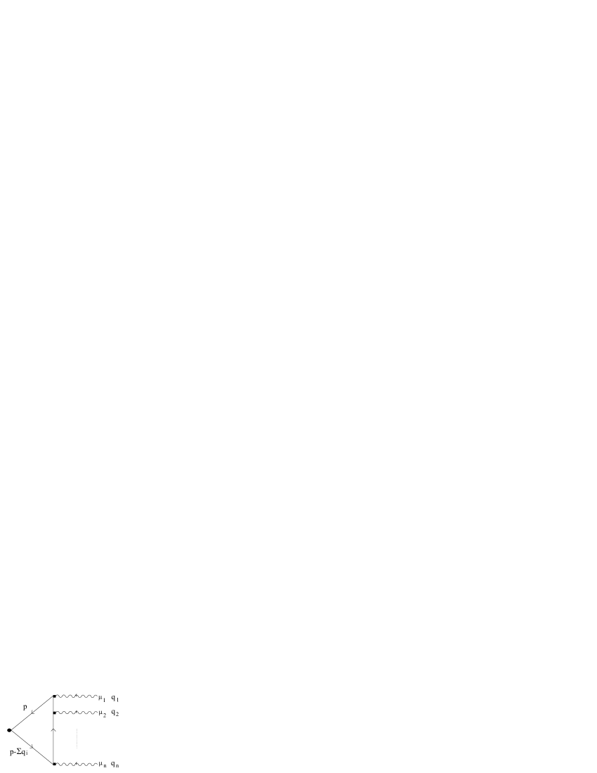
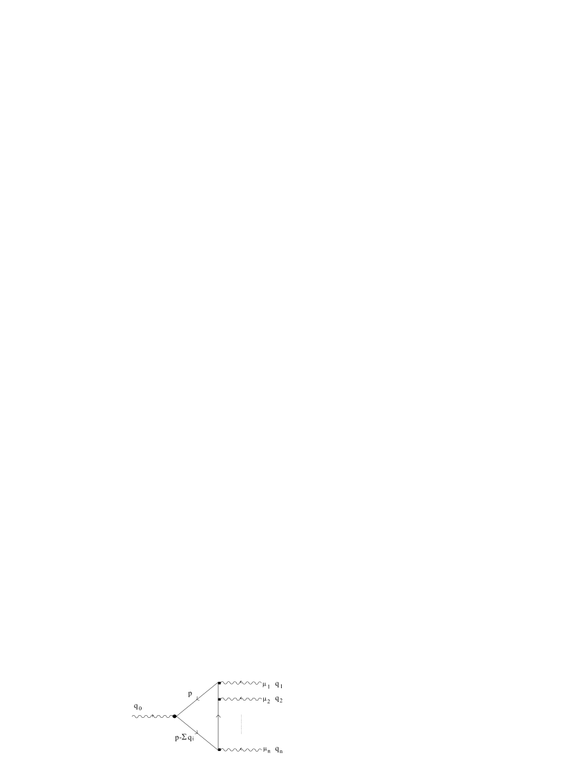
Fig. 1: Diagrams that give the r.h.s of eq. (3.38).

With the help of the Feynman rules in the Appendix A, we conclude that the Feynman diagram in Fig. 1a) represents the following Feynman integral

$$\begin{array}[]{l}{{\mathfrak{A}}_{n}\,=\,N_{f}\,\frac{2(-1)^{n}}{n!}\,e^{\frac{i}{2}\,h\,\sum_{i>j}{q_{i}\circ q_{j}}}\text{Tr}\,A_{\mu_{1}}(q_{1})A_{\mu_{2}}(q_{2})\dots A_{\mu_{n}}(q_{n})}\\ {\phantom{{\mathfrak{A}}_{n}\,=\,\frac{2(-1)^{n}}{n!}e^{\frac{i}{2}\,h\,\sum_{i>j}{q_{i}\circ q_{j}}}A_{\mu_{1}}}\int\!\frac{d^{D}\!p}{(2\pi)^{D}}\,\,\text{tr}\frac{\gamma_{5}\hat{{p\mkern-7.0mu/}}{p\mkern-7.0mu/}\gamma^{\mu_{1}}({p\mkern-7.0mu/}-{q\mkern-7.0mu/}_{1})\gamma^{\mu_{2}}({p\mkern-7.0mu/}-{q\mkern-7.0mu/}_{1}-{q\mkern-7.0mu/}_{2})\dots\gamma^{\mu_{n}}\left({p\mkern-7.0mu/}-\sum{{q\mkern-7.0mu/}_{i}}\right)}{p^{2}(p-q_{1})^{2}(p-q_{q}-q_{2})^{2}\dots\left(p-\sum{q_{i}}\right)^{2}}.}\\ \end{array}$$ (3.40)

The Feynman diagram in Fig. 1b) yields the following Feynman integral

$$\begin{array}[]{l}{{\mathfrak{B}}_{n}\,=\,N_{f}\,\frac{2(-1)^{n}}{n!}\,e^{\frac{i}{2}\,h\,\sum_{i>j}{q_{i}\circ q_{j}}}\text{Tr}A_{\mu}(q_{0})A_{\mu_{1}}(q_{1})A_{\mu_{2}}(q_{2})\dots A_{\mu_{n}}(q_{n})}\\ {\phantom{{\mathfrak{B}}_{n}\equiv\frac{2(-1)^{n}}{n!}\,e^{\frac{i}{2}\,h\,\sum_{i>j}{q_{i}\circ q_{j}}}}\int\!\frac{d^{D}\!p}{(2\pi)^{D}}\,\,\text{tr}\frac{\gamma_{5}\hat{\gamma^{\mu}}{p\mkern-7.0mu/}\gamma^{\mu_{1}}({p\mkern-7.0mu/}-{q\mkern-7.0mu/}_{1})\gamma^{\mu_{2}}({p\mkern-7.0mu/}-{q\mkern-7.0mu/}_{1}-{q\mkern-7.0mu/}_{2})\dots\gamma^{\mu_{n}}\left({p\mkern-7.0mu/}-\sum{{q\mkern-7.0mu/}_{i}}\right)}{p^{2}(p-q_{1})^{2}(p-q_{q}-q_{2})^{2}\dots\left(p-\sum{q_{i}}\right)^{2}}.}\\ \end{array}$$ (3.41)

In eqs. (3.40) and (3.41), we have used $q_{i}\circ q_{j}$ as shorthand for $\theta^{\mu\nu}\,q_{\mu\,i}q_{\mu\,j}$. Note that from the point of view of its $\theta^{\mu\nu}$-dependence the diagrams in Fig. 1 are planar diagrams. Hence, no loop momenta is contracted with $\theta^{\mu\nu}$ in the corresponding Feynman integrals. This feature of the diagrams contributing to the r.h.s. of eq. (3.38) makes it feasible their computation at any order in $h$. Let us remark that in keeping with the general strategy adopted in this paper the exponentials involving $h\,\theta^{\mu\nu}$ are always understood as given by their expansions in powers of $h$.

It turns out that the UV degree of divergence at $D=4$ of the integral that is obtained from ${\mathfrak{A}}_{n}$ by replacing $\hat{{p\mkern-7.0mu/}}$ with ${p\mkern-7.0mu/}$ is negative if $n>4$. Then, for $n>4$, ${\mathfrak{A}}_{n}$ vanishes as $D\rightarrow 4$. The same type of power-counting arguments can be applied to ${\mathfrak{B}}_{n}$, to conclude that these integrals, if $n>3$, go to zero as $D\rightarrow 4$. Now, using the trace identities in eq. (B.99), one easily shows that ${\mathfrak{A}}_{1}={\mathfrak{B}}_{1}=0$. After a little Dirac algebra, one can show that the contributions to ${\mathfrak{B}}_{2}$ and ${\mathfrak{B}}_{3}$ that involve integrals that are not finite by power-counting at $D=4$ are all proportional to contractions of the type $\hat{g}_{\mu\nu}\epsilon^{\nu\rho\lambda\sigma}$. Since these contractions vanish –see eq. (B.98)–, we have ${\mathfrak{B}}_{2}={\mathfrak{B}}_{3}=0$. In summary, in the limit $D\rightarrow 4$, only ${\mathfrak{A}}_{2}$, ${\mathfrak{A}}_{3}$ and ${\mathfrak{A}}_{4}$ may give contributions to the r.h.s. of eq. (3.38), and, indeed, they do so. After some Dirac algebra –see Appendix B– and with the help of the integrals in Appendix C, one obtains the following results for ${\mathfrak{A}}_{2}$, ${\mathfrak{A}}_{3}$ and ${\mathfrak{A}}_{4}$ in position space and in the dimensional regularization minimal subtraction scheme:

$$\begin{array}[]{l}{{\mathfrak{A}}_{2}=-\frac{N_{f}}{8\pi^{2}}\epsilon^{{\mu_{1}}{\mu_{2}}{\mu_{3}}{\mu_{4}}}\text{Tr}\,{\partial}_{\mu_{1}}A_{\mu_{2}}\star{\partial}_{\mu_{3}}A_{\mu_{4}},}\\ {{\mathfrak{A}}_{3}=-i\frac{N_{f}}{4\pi^{2}}\epsilon^{{\mu_{1}}{\mu_{2}}{\mu_{3}}{\mu_{4}}}\,\text{Tr}\,\left[{\partial}_{\mu_{4}}A_{\mu_{1}}\star A_{\mu_{2}}\star A_{\mu_{3}}+A_{\mu_{1}}\star A_{\mu_{2}}\star{\partial}_{\mu_{4}}A_{\mu_{3}}\right],}\\ {{\mathfrak{A}}_{4}=\frac{N_{f}}{4\pi^{2}}\,\epsilon^{{\mu_{1}}{\mu_{2}}{\mu_{3}}{\mu_{4}}}\,\,\text{Tr}\,A_{\mu_{1}}\star A_{\mu_{2}}\star A_{\mu_{3}}\star A_{\mu_{4}}.}\\ \end{array}$$ (3.42)

Substituting eq. (3.42) in the r.h.s. of eq. (3.39), one gets

$$\sum_{i}\,({\mathfrak{D}}_{\mu}\,<j_{5}^{(p)\;\mu}>^{(A)}_{\rm MS})_{ii}\,=\,\frac{N_{f}}{16\pi^{2}}\epsilon^{{\mu_{1}}{\mu_{2}}{\mu_{3}}{\mu_{4}}}\,\text{Tr}\,F_{{\mu_{1}}{\mu_{2}}}\star F_{{\mu_{3}}{\mu_{4}}}.$$ (3.43)

This equation looks like the corresponding equation for $U(N)$ groups –see eq. (9b) in ref. [26]. This similarity comes from the fact that in both cases no loop momenta is contracted with $\theta^{\mu\nu}$, and currents and interaction vertices are the same type of polynomials with respect to the Moyal product. However, there are two striking differences. First, the theory in ref. [26] need not be defined by means of the Seiberg-Witten map, but the theory considered in this paper is unavoidably constructed by using the Seiberg-Witten map. Secondly, the object $F_{{\mu_{1}}{\mu_{2}}}$ belongs to the Lie algebra of $U(N)$ in the theory of ref. [26], whereas it belongs to the enveloping algebra of $SU(N)$, not to its Lie algebra, in the case studied here.

Eq. (3.43) leads to the conclusion that, at least at the one-loop level, the classical conservation equation for $j_{5}^{(p)\;\mu}$ in eq. (3.31) should be replaced with

$$\sum_{i}\,({\mathfrak{D}}_{\mu}\,{\rm N}[j_{5}^{(p)\;\mu}]_{\rm MS})_{ii}\,=\,\frac{N_{f}}{8\pi^{2}}\,\text{Tr}\,F_{{\mu_{1}}{\mu_{2}}}\star\tilde{F}_{{\mu_{3}}{\mu_{4}}},$$ (3.44)

where ${\rm N}[\phantom{j_{5}}]_{\rm MS}$ denotes normal product of operators in the MS scheme [53, 55] and $\tilde{F}^{{\mu_{1}}{\mu_{2}}}=\frac{1}{2}\epsilon^{{\mu_{1}}{\mu_{2}}{\mu_{3}}{\mu_{4}}}F_{{\mu_{3}}{\mu_{4}}}$. Eq. (3.44) tell us that for commutative time, i.e., $\theta^{0i}=0$, the charge $Q_{5}^{(p)}$ is no longer conserved but verifies the following anomalous equation

$$Q_{5}^{(p)}(t=+\infty)-Q_{5}^{(p)}(t=-\infty)\,=\,\frac{N_{f}}{8\pi^{2}}\int\!d^{4}\!x\,\,\text{Tr}\,F_{{\mu_{1}}{\mu_{2}}}\star\tilde{F}_{{\mu_{3}}{\mu_{4}}}.$$ (3.45)

The charge $Q_{5}^{(p)}(t)$ was defined in eq. (2.23). To obtain the l.h.s. of the previous equation, we have integrated the l.h.s of eq. (3.44) and assumed that the fields vanish fast enough at spatial infinity so as to make the following identity

$$\int\,d^{3}\vec{x}\;(\Phi_{1}\star\Phi_{2})(t,\vec{x})\,=\,\int\,d^{3}\vec{x}\;\Phi_{1}(t,\vec{x})\Phi_{2}(t,\vec{x})$$

valid for $\theta^{\mu\nu}$ such that $\theta^{0i}=0$. This choice of asymptotic behaviour is standard in noncommutative field theory  [9, 10, 11] and renders the kinetic terms of the fields in ordinary and noncommutative space-time equal.

Using the techniques in [38], it is not difficult to show that

$$\int\!d^{4}\!x\,\,\text{Tr}\,F_{{\mu_{1}}{\mu_{2}}}\star\tilde{F}_{{\mu_{3}}{\mu_{4}}}\,=\,\int\!d^{4}\!x\,\,\text{Tr}\,f_{{\mu_{1}}{\mu_{2}}}\tilde{f}_{{\mu_{3}}{\mu_{4}}},$$

at least for the boundary conditions in eq. (2.27). This equation was obtained for the $U(1)$ gauge group in ref. [56]. Now, by combining the previous equation with eq. (3.45), and, then, using the temporal gauge and the boundary conditions in eq. (2.27), one concludes that

$$Q_{5}^{(p)}(t=+\infty)-Q_{5}^{(p)}(t=-\infty)\,=\,\frac{N_{f}}{8\pi^{2}}\int\!d^{4}\!x\,\,\text{Tr}\,f_{{\mu_{1}}{\mu_{2}}}\tilde{f}_{{\mu_{3}}{\mu_{4}}}\,=\,2\,N_{f}\,(n_{+}-n_{-}).$$ (3.46)

The integers $n_{\pm}$ are defined in eq. (2.28).

3.2 Anomalous Ward identity for $j_{5}^{(np)\;\mu}$

The variation of $S[\Psi_{f},\bar{\Psi}_{f},A]_{Fermi}^{DR}$ in eq. (3.35) under the chiral transformations

$$\quad\quad\delta\Psi_{f}\,=\,-i\gamma_{5}\Psi_{f}\star\alpha\quad\delta\bar{\Psi}_{f}\,=\,-i\alpha\star\bar{\Psi}_{f}\gamma_{5}$$

reads

$$\delta S_{Fermi}^{DR}\,=\,-\int\!\!d^{D}\!x\,\big{[}(\partial_{\mu}\,j_{5}^{(np)\;\mu})(x)-2\sum_{f}\,(\bar{\Psi}_{f}\star{\hat{\gamma}}^{\mu}\gamma_{5}\gamma_{5}\Psi_{f})(x)\big{]}\,\alpha(x).$$

Now, $Z[A]$ in eqs. (3.37) is invariant under the previous chiral transformations. That $\delta Z[A]=0$ and that $\delta S_{Fermi}^{DR}$ be given by the previous expression leads to

$$\partial_{\mu}<j_{5}^{(np)\;\mu}>^{(A)}(x)=2\,\sum_{f}\,<\bar{\Psi}_{f}\star{\hat{\gamma}}^{\mu}\gamma_{5}D_{\mu}\Psi_{f}>^{(A)}(x).$$ (3.47)

The v.e.v. in the noncommutative background $A$, $<\cdots>^{(A)}$, is defined by the last line of eq. (3.36), which in dimensional regularization is equivalent to the original definition in eq. (3.33). Note that either side of eq. (3.47) is invariant under $SU(N)$ gauge transformations of $a_{\mu}$, here the MS scheme algorithm of dimensional regularization will yield a gauge invariant result when applied to either side of that equation.

The r.h.s. of eq. (3.47) contains an evanescent operator, which upon MS dimensional renormalization will give a finite contribution when inserted in UV divergent fermion loops. In this subsection we will compute this finite contribution up to second order in $h$. At first order in $h$, we shall work out every Feynman diagram giving, in the $D\rightarrow 4$ limit, a nonvanishing contribution to the r.h.s. of eq. (3.47). To make this computation feasible at order $h^{2}$, we will take advantage of the gauge invariance of the result and compute explicitly only the minimum number of Feynman diagrams needed. Let us show next that if we have a gauge invariant expression, say ${\cal A}^{(2)}[a_{\mu}]$, that matches the contribution obtained by explicit computation of the diagrams involving fewer than five fields $a_{\mu}$, then there is no room for the Feynman diagrams with five or more fields $a_{\mu}$ giving a contribution not included in ${\cal A}^{(2)}$. The standard BRS transformations reads:

$$sa^{a}_{\mu}=s_{0}a^{a}_{\mu}-s_{1}a^{a}_{\mu},\quad s_{0}a^{a}_{\mu}=\partial_{\mu}c^{a},\quad s_{1}a^{a}_{\mu}=-if^{abc}a^{b}_{\mu}c^{c},\quad\quad sc^{a}=if^{abc}c^{b}c^{c}.$$ (3.48)

Then, the gauge invariance of ${\cal A}^{(2)}[a_{\mu}]$, $s{\cal A}^{(2)}=0$, is equivalent to the following set of equations

$$\begin{array}[]{l}{s_{0}{\cal A}^{(2)}_{2}\,=\,0,}\\ {s_{0}{\cal A}^{(2)}_{3}\,=\,s_{1}{\cal A}^{(2)}_{2},}\\ {s_{0}{\cal A}^{(2)}_{4}\,=\,s_{1}{\cal A}^{(2)}_{3},}\\ {s_{0}{\cal A}^{(2)}_{5}\,=\,s_{1}{\cal A}^{(2)}_{4},}\\ {s_{0}{\cal A}^{(2)}_{6}\,=\,s_{1}{\cal A}^{(2)}_{5},}\\ {s_{0}{\cal A}^{(2)}_{7}\,=\,s_{1}{\cal A}^{(2)}_{6},}\\ {s_{0}{\cal A}^{(2)}_{8}\,=\,s_{1}{\cal A}^{(2)}_{7},}\\ {s_{1}{\cal A}^{(2)_{8}}\,=\,0.}\\ \end{array}$$ (3.49)

The symbol ${\cal A}^{(2)}_{n}$, $n=2,3,4,5,6,7$ and $8$, denotes the contribution to ${\cal A}^{(2)}[a_{\mu}]$ involving $n$ fields, and its derivatives, $a_{\mu}$:

$${\cal A}^{(2)}[a_{\mu}]\,=\,\sum_{n=2}^{8}\;{\cal A}^{(2)}_{n}[a_{\mu}].$$

Dimensional analysis shows that $n<9$. Indeed, ${\cal A}^{(2)}_{n}$ has dimension 4 and ${\cal A}^{(2)}_{n}=h^{2}\,\theta^{\mu_{1}\mu_{2}}\theta^{\mu_{3}\mu_{4}}f_{\mu_{1}\mu_{2}\mu_{3}\mu_{4}}[a_{\mu}]$, $f_{\mu_{1}\mu_{2}\mu_{3}\mu_{4}}[a_{\mu}]$ being a gauge invariant polynomial of $a_{\mu}$ and its derivatives. The fact that the generators of a unitary representation of $SU(N)$ are traceless implies that $n>1$. Let ${\cal B}^{(2)}=h^{2}\,\theta^{\mu_{1}\mu_{2}}\theta^{\mu_{3}\mu_{4}}g_{\mu_{1}\mu_{2}\mu_{3}\mu_{4}}[a_{\mu}]$ be a gauge invariant –i.e., $s{\cal B}^{(2)}=0$– polynomial of $a_{\mu}$ and its derivatives which is equal to ${\cal A}^{(2)}$ up to contributions with more than four $a_{\mu}$, or derivatives of it, and has dimension 4:

$${\cal B}^{(2)}\,=\,\sum_{n=2}^{4}\;{\cal A}^{(2)}_{n}[a_{\mu}]\,+\,\sum_{n=5}^{8}\;{\cal B}^{(2)}_{n}[a_{\mu}].$$

${\cal B}^{(2)}_{n}$ denotes the contribution involving $n$ fields $a_{\mu}$, or derivatives of it. Let ${\cal C}^{(2)}_{n}$ stand for the difference ${\cal A}^{(2)}_{n}-{\cal B}^{(2)}_{n}$, $n=5,6,7$ and $8$. Then, the BRS invariance of both ${\cal A}^{(2)}$ and ${\cal B}^{(2)}$ –use eq. (3.49)– leads to

$$\begin{array}[]{l}{s_{0}{\cal C}^{(2)}_{5}\,=\,0,}\\ {s_{0}{\cal C}^{(2)}_{6}\,=\,s_{1}{\cal C}^{(2)}_{5},}\\ {s_{0}{\cal C}^{(2)}_{7}\,=\,s_{1}{\cal C}^{(2)}_{6},}\\ {s_{0}{\cal C}^{(2)}_{8}\,=\,s_{1}{\cal C}^{(2)}_{7},}\\ {s_{1}{\cal C}^{(2)}_{8}\,=\,0.}\\ \end{array}$$ (3.50)

Now, the cohomology of the operator $s_{0}$ over the space of polynomials of $a^{a}_{\mu}$, $c^{a}$ and their derivatives has been worked out in refs. [57, 58]. The nontrivial part of this cohomology is given by polynomials of $f^{a\,(free)}_{\mu\nu}=\partial_{\mu}a^{a}_{\nu}-\partial_{\nu}a^{a}_{\mu}$ and/or its derivatives and/or $c^{a}$. Since ${\cal C}^{(2)}_{5}$ belongs to the nontrivial part of the cohomology of $s_{0}$ and does not depends on $c^{a}$, we conclude that it should be either zero or a polynomial of $f^{a\,(free)}_{\mu\nu}$ and its derivatives. This last possibility will never be realized in the case under scrutiny since one can show by dimensional analysis that ${\cal C}^{(2)}_{5}$ can contain only two partial derivatives, i.e., ${\cal C}^{(2)}_{5}$ must be a linear combination of monomials of the type $\partial_{\mu}a^{a}_{\nu}\partial_{\rho}a^{b}_{\sigma}a^{c}_{\nu_{1}}a^{d}_{\nu_{2}}a^{e}_{\nu_{3}}$ and/or of the form $\partial_{\mu}\partial_{\rho}a^{a}_{\nu}a^{b}_{\sigma}a^{c}_{\nu_{1}}a^{d}_{\nu_{2}}a^{e}_{\nu_{3}}$. We have thus shown that ${\cal C}^{(2)}_{5}$ actually vanishes. Substituting, this result in eq. (3.50), one obtains the following equation for ${\cal C}^{(2)}_{6}$: $s_{0}\,{\cal C}^{(2)}_{6}=0$. The same kind of analysis that yielded a vanishing ${\cal C}^{(2)}_{5}=0$ leads to the conclusion that ${\cal C}^{(2)}_{6}=0$. And so on, and so forth. We have thus shown that ${\cal C}^{(2)}_{n}=0$ for all $n$. Hence, ${\cal A}^{(2)}={\cal B}^{(2)}$. Notice that our strategy would have failed if we had decided not to compute diagrams with four gauge fields (or derivatives of it) $a_{\mu}$. Indeed, $s_{0}\,{\cal C}^{(2)}_{4}=0$, with ${\cal C}^{(2)}_{4}={\cal A}^{(2)}_{4}-{\cal B}^{(2)}_{4}$, does not imply ${\cal C}^{(2)}_{4}=0$, since ${\cal C}^{(2)}_{4}$ may be a nonvanishing linear combination of monomials of the type $f^{a_{1}\,(free)}_{\mu_{1}\nu_{1}}f^{a_{2}\,(free)}_{\mu_{2}\nu_{2}}f^{a_{3}\,(free)}_{\mu_{3}\nu_{3}}f^{a_{4}\,(free)}_{\mu_{4}\nu_{4}}$.

The Feynman integrals that yield the r.h.s of eq. (3.47) at order $h^{n}$ can be worked out by extracting the contribution of this order coming from the “master” Feynman diagrams in Fig. 2. The dimensionally regularized object that these diagrams represent can be obtained by using the Feyman rules in Appendix A. In these rules and in all our expressions the exponentials $e^{i\frac{h}{2}k_{1}\circ k_{2}}$, with $k_{1}\circ k_{2}=\theta^{\mu\nu}k_{1\,\mu}\,k_{2\,\mu}$, are actually shorthand for their series expansions $\sum_{n=0}^{\infty}\,\frac{i^{n}h^{n}}{2^{n}n!}\,(k_{1}\circ k_{2})^{n}$.

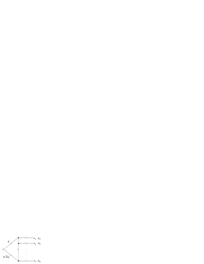
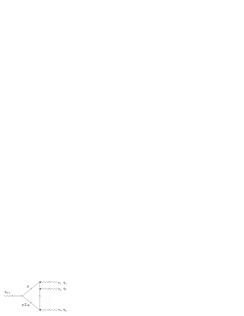
Fig. 2: Diagrams that give the r.h.s of eq. (3.47).

The “master” Feynman diagram in Fig. 2a represents the following object:

$$\begin{array}[]{l}{{\mathfrak{F}}_{n}\,=\,N_{f}\,\frac{2(-1)^{n+1}}{n!}\,e^{\frac{i}{2}\,h\,(\sum_{i>j}{q_{i}\circ q_{j}})\,}\text{Tr}\,A_{\mu_{1}}(q_{1})A_{\mu_{2}}(q_{2})\dots A_{\mu_{n}}(q_{n})}\\ {\phantom{A_{n}\,=\,\frac{2(-1)}{n!}}\sum_{m=0}^{\infty}\frac{i^{m}h^{m}}{m!}\,\int\!\frac{d^{D}\!p}{(2\pi)^{D}}\,\,\,(\sum_{k}p\circ q_{k})^{m}\;\text{tr}\frac{\gamma^{5}\hat{{p\mkern-7.0mu/}}{p\mkern-7.0mu/}\gamma^{\mu_{1}}({p\mkern-7.0mu/}-{q\mkern-7.0mu/}_{1})\gamma^{\mu_{2}}({p\mkern-7.0mu/}-{q\mkern-7.0mu/}_{1}-{q\mkern-7.0mu/}_{2})\dots\gamma^{\mu_{n}}\left({p\mkern-7.0mu/}-\sum_{i}{q\mkern-7.0mu/}_{i}\right)}{p^{2}(p-q_{1})^{2}(p-q_{q}-q_{2})^{2}\dots\left(p-\sum_{i}q_{i}\right)^{2}}.}\\ \end{array}$$ (3.51)

The “master” Feynman diagram in Fig. 2b corresponds to the expression that follows:

$$\begin{array}[]{l}{{\mathfrak{G}}_{n}\,=\,N_{f}\,\frac{2(-1)^{n+1}}{n!}\,e^{\frac{i}{2}\,h\,(\sum_{i>j}q_{i}\circ q_{j})}\;\text{Tr}A_{\mu}(q_{n+1})A_{\mu_{1}}(q_{1})A_{\mu_{2}}(q_{2})\dots A_{\mu_{n}}(q_{n})}\\ {\phantom{{\mathfrak{E}}_{n}\,=\,\frac{2(-1)}{n!}}\sum_{m=0}^{\infty}\frac{i^{m}h^{m}}{m!}\,\int\!\frac{d^{D}\!p}{(2\pi)^{D}}\,\,\,(\sum_{k}p\circ q_{k})^{m}\;\text{tr}\frac{\gamma^{5}\hat{\gamma^{\mu}}{p\mkern-7.0mu/}\gamma^{\mu_{1}}({p\mkern-7.0mu/}-{q\mkern-7.0mu/}_{1})\gamma^{\mu_{2}}({p\mkern-7.0mu/}-{q\mkern-7.0mu/}_{1}-{q\mkern-7.0mu/}_{2})\dots\gamma^{\mu_{n}}\left({p\mkern-7.0mu/}-\sum_{i}{q\mkern-7.0mu/}_{i}\right)}{p^{2}(p-q_{1})^{2}(p-q_{q}-q_{2})^{2}\dots\left(p-\sum_{i}q_{i}\right)^{2}}.}\\ \end{array}$$ (3.52)

Let us see first that the MS dimensional renormalization algorithm [52, 53, 55] sets to zero at $D=4$ any contribution coming from ${\mathfrak{G}}_{n}$ in eq. (3.52). Using the identities in eqs. (B.98) and (B.99), one can work out the trace over the the gamma matrices and show that

$$\begin{array}[]{l}{\text{tr}\gamma^{5}\hat{\gamma^{\mu}}{p\mkern-7.0mu/}\gamma^{\mu_{1}}({p\mkern-7.0mu/}-{q\mkern-7.0mu/}_{1})\gamma^{\mu 2}({p\mkern-7.0mu/}-{q\mkern-7.0mu/}_{1}-{q\mkern-7.0mu/}_{2})\dots\gamma^{\mu_{n}}\left({p\mkern-7.0mu/}-\sum{{q\mkern-7.0mu/}_{i}}\right)}\\ {=\hat{p}^{\mu}T_{1}^{\mu_{1}\dots\mu_{n}}+\sum_{i}\hat{g}^{\mu\mu_{i}}T_{2\,i}^{\mu_{1}\dots\mu_{i-1}\mu_{i+1}\dots\mu_{n}}+\sum_{i}\hat{q}_{i}^{\mu}T_{3\,i}^{\mu_{1}\dots\mu_{n}}.}\\ \end{array}$$

$T_{1}$, $T_{2\,i}$ and $T_{3\,i}$ are “Lorentz covariant tensors” in the $D$-dimensional space-time of dimensional regularization. The expression on the r.h.s. of the previous equation shows that any contribution coming from ${\mathfrak{G}}_{n}$ that does not vanish as $D\rightarrow 4$ matches one of the following “tensor” patterns

$$\begin{array}[]{l}{\frac{1}{D-4}\,t_{1}^{\mu_{1}\dots\mu_{n}}\,\text{Tr}\,A_{\mu_{1}}(q_{1})\dots\hat{A}_{\mu_{k}}(q_{k})\dots A_{\mu_{n}}(q_{n}),}\\ {\frac{1}{D-4}\,t_{2}^{\nu\mu_{1}\dots\mu_{n}}\,\text{Tr}\,\hat{q}_{i\,\nu}A_{\mu_{1}}(q_{1})\dots A_{\mu_{i}}(q_{i})\cdots A_{\mu_{n}}(q_{n}).}\end{array}$$ (3.53)

It is important to bear in mind that $t_{1}^{\mu_{1}\dots\mu_{n}}$ and $t_{2}^{\nu\mu_{1}\dots\mu_{n}}$ must be linear combinations of “Lorentz covariant tensors” with coefficients that do not depend on $(D-4)$. For instance, a “tensor” like $t_{1}^{\mu_{1}\dots\mu_{6}}=(D-4)\,\epsilon^{\mu_{1}\mu_{2}\mu_{3}\mu_{4}}g^{\mu_{5}\mu_{6}}$ is not to be admitted, for this type of $t_{1}$ tensor, when substituted back in the first equality in eq. (3.53), yields a contribution that does not go to zero as $D\rightarrow 4$. Now, the MS dimensional regularization algorithm removes from ${\mathfrak{G}}_{n}$ any contribution of the types shown in eq. (3.53). Every ${\mathfrak{G}}_{n}$ is thus renormalized to zero at $D=4$ in the MS renormalization scheme.

The identities in eqs. (B.98) and (B.99) can be used to remove from ${\mathfrak{F}}_{n}$ any term that upon MS renormalization will go away as $D\rightarrow 4$. The trace over the Dirac matrices of ${\mathfrak{F}}_{n}$ in eq. (3.51) is given by

$$\begin{array}[]{l}{\text{tr}\gamma^{5}\hat{{p\mkern-7.0mu/}}{p\mkern-7.0mu/}\gamma^{\mu_{1}}({p\mkern-7.0mu/}-{q\mkern-7.0mu/}_{1})\gamma^{\mu 2}({p\mkern-7.0mu/}-{q\mkern-7.0mu/}_{1}-{q\mkern-7.0mu/}_{2})\dots\gamma^{\mu_{n}}\left({p\mkern-7.0mu/}-\sum{{q\mkern-7.0mu/}_{i}}\right)}\\ {=\hat{p}^{2}\,R^{\mu_{1}\dots\mu_{n}}+\sum_{i}\hat{p}^{\mu_{i}}\,S_{i}^{\mu_{1}\dots\mu_{i-1}\mu_{i+1}\dots\mu_{n}}+\sum_{i}\hat{p}\cdot q_{i}\,T^{\mu_{1}\dots\mu_{n}}.}\\ \end{array}$$ (3.54)

$R$, $S$ and $T$ are also “Lorentz covariant tensors” in the $D$-dimensional space-time of dimensional regularization. Redoing the analysis that begun just below eq. (3.52) for the case at hand –mutatis mutandi–, one shows that the contributions that go with the “tensors” $S$ and $T$ in eq. (3.54) can be dropped. This is so since, after MS renormalization, they will go to zero as $D\rightarrow 4$. Hence, upon MS renormalization, all nonvanishing contributions at $D=4$ coming from ${\mathfrak{F}}_{n}$ in eq. (3.51) will be furnished by the term $\hat{p}^{2}\,R^{\mu_{1}\dots\mu_{n}}$ in eq. (3.54). And yet, these contributions will also vanish as $D\rightarrow 4$ unless the integration over $p$ yields a pole at $D=4$ when $\hat{p}^{2}$ is replaced with $p_{\mu}p_{\nu}$. Now, make the latter replacement in the integrals of ${\mathfrak{F}}_{n}$. Then, some power-counting at $D=4$ tell us that all the integrals thus obtained are UV finite if our ${\mathfrak{F}}_{n}$ is such that $n>4+m$ –this $m$ indicates that we are dealing with a term of order $h^{m}$. After contraction with $\hat{g}^{\mu\nu}$, these integrals will vanish at $D=4$. In summary, to compute, at order $h^{m}$, the nonzero contribution to the MS renormalized r.h.s. of eq. (3.47), only the values of the ${\mathfrak{F}}_{n}$ objects verifying

$${\mathfrak{F}}_{n}\quad\text{such that}\quad n\leq m+4$$ (3.55)

are actually needed.

We shall denote by $2\,\sum_{f}\,<\bar{\Psi}_{f}\star{\hat{\gamma}}^{\mu}\gamma_{5}D_{\mu}\Psi_{f}>^{(A)}_{MS}$ the renormalized object obtained by applying to the r.h.s eq. (3.47) the minimal subtraction algorithm of dimensional regularization. This object is to be understood as an expansion in $h$:

$$2\,\sum_{f}\,<\bar{\Psi}_{f}\star{\hat{\gamma}}^{\mu}\gamma_{5}D_{\mu}\Psi_{f}>^{(A)}_{MS}\,=\,{\cal A}^{(0)}\,+\,h\,{\cal A}^{(1)}\,+\,h^{2}\,{\cal A}^{(2)}\,+\,o(h^{3}).$$ (3.56)

${\cal A}^{(0)}$ is given by the well known ordinary $U(1)_{A}$ anomaly:

$$\frac{N_{f}}{8\pi^{2}}\int\!d^{4}\!x\,\,\text{Tr}\,f_{{\mu_{1}}{\mu_{2}}}\tilde{f}_{{\mu_{3}}{\mu_{4}}}.$$ (3.57)

3.2.1 The computation of ${\cal A}^{(1)}$

According to eq. (3.55), we shall need the ${\mathfrak{F}}_{n}$’s in eq. (3.51) with $n\leq 5$. We will sort out the contributions coming from these ${\mathfrak{F}}_{n}$’s into two categories. The first type of contributions will be obtained by removing from the infinite sum $\sum_{m=0}^{\infty}$ in ${\mathfrak{F}}_{n}$ any term with $m>0$. Hence, the first type of contributions will be furnished by the terms of order $h$ in $-{\mathfrak{A}}_{n}$, ${\mathfrak{A}}_{n}$ being given in eq. (3.40). We thus conclude that the terms in ${\cal A}^{(1)}$ that constitute the first category can be computed by expanding at first order in $h$ the r.h.s. of eq. (3.43):

$$\begin{array}[]{l}{\frac{N_{f}}{16\pi^{2}}\,\epsilon^{{\mu_{1}}{\mu_{2}}{\mu_{3}}{\mu_{4}}}\,\text{Tr}\,F_{{\mu_{1}}{\mu_{2}}}\star F_{{\mu_{3}}{\mu_{4}}}\mid_{h}=-\frac{N_{f}}{4\pi^{2}}\,\theta^{\rho\sigma}\,\epsilon^{\mu_{1}\mu_{2}\mu_{3}\mu_{4}}\Big{\{}\text{Tr}\,[{\partial}_{\mu_{1}}a_{\rho}\partial_{\sigma}a_{\mu_{2}}{\partial}_{\mu_{3}}a_{\mu_{4}}\!+\!a_{\rho}{\partial}_{\mu_{1}}\partial_{\sigma}a_{\mu_{2}}{\partial}_{\mu_{3}}a_{\mu_{4}}}\\ {\phantom{\frac{N_{f}}{16\pi^{2}}\,\epsilon^{{\mu_{1}}{\mu_{2}}{\mu_{3}}}}+{\partial}_{\mu_{1}}\partial_{\sigma}a_{\mu_{2}}a_{\rho}{\partial}_{\mu_{3}}a_{\mu_{4}}+\partial_{\sigma}a_{\mu_{2}}{\partial}_{\mu_{1}}a_{\rho}{\partial}_{\mu_{3}}a_{\mu_{4}}-{\partial}_{\mu_{1}}a_{\rho}{\partial}_{\mu_{2}}a_{\sigma}{\partial}_{\mu_{3}}a_{\mu_{4}}+{\partial}_{\mu_{4}}a_{\mu_{1}}{\partial}_{\rho}a_{\mu_{2}}{\partial}_{\sigma}a_{\mu_{3}}]}\\ {\phantom{\frac{N_{f}}{16\pi^{2}}\,\epsilon^{{\mu_{1}}{\mu_{2}}{\mu_{3}}}}-\frac{i}{2}\,\text{Tr}\,[-a_{\sigma}a_{\mu_{1}}{\partial}_{\mu_{2}}a_{\mu_{3}}{\partial}_{\mu_{4}}a_{\rho}-2a_{\sigma}a_{\rho}{\partial}_{\mu_{1}}a_{\mu_{2}}{\partial}_{\mu_{3}}a_{\mu_{4}}-2a_{\sigma}a_{\mu_{3}}{\partial}_{\mu_{4}}a_{\rho}{\partial}_{\mu_{1}}a_{\mu_{2}}}\\ {\phantom{\frac{N_{f}}{16\pi^{2}}\,\epsilon^{{\mu_{1}}{\mu_{2}}{\mu_{3}}}+\frac{i}{2}\,\text{Tr}\,[}-a_{\sigma}{\partial}_{\mu_{1}}a_{\rho}a_{\mu_{2}}{\partial}_{\mu_{3}}a_{\mu_{4}}+a_{\sigma}{\partial}_{\mu_{3}}a_{\mu_{4}}a_{\mu_{2}}{\partial}_{\mu_{1}}a_{\rho}-2a_{\sigma}{\partial}_{\mu_{3}}a_{\mu_{4}}{\partial}_{\mu_{1}}a_{\rho}a_{\mu_{2}}}\\ {\phantom{\frac{N_{f}}{16\pi^{2}}\,\epsilon^{{\mu_{1}}{\mu_{2}}{\mu_{3}}}+\frac{i}{2}\,\text{Tr}\,[}-a_{\sigma}{\partial}_{\mu_{1}}a_{\rho}{\partial}_{\mu_{3}}a_{\mu_{4}}a_{\mu_{2}}-2{\partial}_{\sigma}a_{\mu_{1}}a_{\mu_{2}}a_{\mu_{3}}{\partial}_{\mu_{4}}a_{\rho}-2{\partial}_{\sigma}a_{\mu_{4}}a_{\rho}a_{\mu_{1}}{\partial}_{\mu_{2}}a_{\mu_{3}}}\\ {\phantom{\frac{N_{f}}{16\pi^{2}}\,\epsilon^{{\mu_{1}}{\mu_{2}}{\mu_{3}}}+\frac{i}{2}\,\text{Tr}\,[}-2{\partial}_{\sigma}a_{\mu_{3}}{\partial}_{\mu_{4}}a_{\rho}a_{\mu_{1}}a_{\mu_{2}}-2{\partial}_{\sigma}a_{\mu_{1}}{\partial}_{\mu_{2}}a_{\mu_{3}}a_{\mu_{4}}a_{\rho}+2{\partial}_{\sigma}a_{\mu_{1}}a_{\mu_{2}}{\partial}_{\mu_{3}}a_{\mu_{4}}a_{\rho}}\\ {\phantom{\frac{N_{f}}{16\pi^{2}}\,\epsilon^{{\mu_{1}}{\mu_{2}}{\mu_{3}}}+\frac{i}{2}\,\text{Tr}\,[}+2{\partial}_{\sigma}a_{\mu_{4}}a_{\rho}{\partial}_{\mu_{1}}a_{\mu_{2}}a_{\mu_{3}}+2{\partial}_{\sigma}{\partial}_{\mu_{1}}a_{\mu_{2}}a_{\mu_{3}}a_{\mu_{4}}a_{\rho}+2{\partial}_{\sigma}{\partial}_{\mu_{3}}a_{\mu_{4}}a_{\rho}a_{\mu_{1}}a_{\mu_{2}}}\\ {\phantom{\frac{N_{f}}{16\pi^{2}}\,\epsilon^{{\mu_{1}}{\mu_{2}}{\mu_{3}}}+\frac{i}{2}\,\text{Tr}\,[}+2{\partial}_{\mu_{4}}a_{\rho}{\partial}_{\mu_{1}}a_{\sigma}a_{\mu_{2}}a_{\mu_{3}}+{\partial}_{\mu_{2}}a_{\sigma}a_{\mu_{3}}{\partial}_{\mu_{4}}a_{\mu_{1}}a_{\rho}+a_{\mu_{3}}{\partial}_{\mu_{4}}a_{\mu_{1}}{\partial}_{\mu_{2}}a_{\sigma}a_{\rho}}\\ {\phantom{\frac{N_{f}}{16\pi^{2}}\,\epsilon^{{\mu_{1}}{\mu_{2}}{\mu_{3}}}+\frac{i}{2}\,\text{Tr}\,[}+{\partial}_{\mu_{3}}a_{\sigma}{\partial}_{\mu_{4}}a_{\mu_{1}}a_{\mu_{2}}a_{\rho}+{\partial}_{\mu_{4}}a_{\mu_{1}}a_{\mu_{2}}{\partial}_{\mu_{3}}a_{\sigma}a_{\rho}+2{\partial}_{\sigma}a_{\mu_{1}}{\partial}_{\rho}a_{\mu_{2}}a_{\mu_{3}}a_{\mu_{4}}]}\\ {\phantom{\frac{N_{f}}{16\pi^{2}}\,\epsilon^{{\mu_{1}}{\mu_{2}}{\mu_{3}}}}+{\partial}_{\mu_{4}}\,\text{Tr}\,[a_{\rho}a_{\sigma}a_{\mu_{1}}a_{\mu_{2}}a_{\mu_{3}}-a_{\rho}a_{\mu_{1}}a_{\sigma}a_{\mu_{2}}a_{\mu_{3}}]\Big{\}}.}\\ \end{array}$$ (3.58)

The second type of contributions that make ${\cal A}^{(1)}$ up are obtained by setting $h$ to zero everywhere in ${\mathfrak{F}}_{n}$, but in the term that goes with $(\sum_{k}\,p\circ q_{k})^{m}$, with $m=1$. These substitutions yield the following expression:

$$\begin{array}[]{l}{{\mathfrak{I}}_{n}\,=\,N_{f}\,\frac{2(-1)^{n+1}}{n!}\,\text{Tr}\,a_{\mu_{1}}(q_{1})a_{\mu_{2}}(q_{2})\dots a_{\mu_{n}}(q_{n})}\\ {\phantom{\frac{2(-1)^{n+1}}{n!}\,a_{\mu_{1}}(q_{1})a_{\mu_{2}}}\int\!\frac{d^{D}\!p}{(2\pi)^{D}}\,\,i(\sum_{k}{p\circ q_{k}})\text{tr}\frac{\gamma^{5}\hat{{p\mkern-7.0mu/}}{p\mkern-7.0mu/}\gamma^{\mu_{1}}({p\mkern-7.0mu/}-{q\mkern-7.0mu/}_{1})\gamma^{\mu_{2}}({p\mkern-7.0mu/}-{q\mkern-7.0mu/}_{1}-{q\mkern-7.0mu/}_{2})\dots\gamma^{\mu_{n}}\left({p\mkern-7.0mu/}-\sum{{q\mkern-7.0mu/}_{i}}\right)}{p^{2}(p-q_{1})^{2}(p-q_{q}-q_{2})^{2}\dots\left(p-\sum{q_{i}}\right)^{2}}.}\\ \end{array}$$

Recall that we saw above that only for $n=2,3,4$ and $5$ may we obtain a nonvanishing output. Using the identity in eq. (3.54), the results in Appendix C and adding the contributions generated by the appropriate permutations of the external momenta, one concludes that ${\mathfrak{I}}_{2}$, ${\mathfrak{I}}_{3}$, ${\mathfrak{I}}_{4}$ and ${\mathfrak{I}}_{5}$ give rise to the following terms in ${\cal A}^{(1)}$:

$$\begin{array}[]{l}{{\mathfrak{I}}_{2}\;\rightsquigarrow\;0,}\\ {{\mathfrak{I}}_{3}\;\rightsquigarrow\;+\frac{N_{f}}{4\pi^{2}}\,\theta^{\rho\sigma}\epsilon^{\mu_{1}\mu_{2}\mu_{3}\mu_{4}}\text{Tr}\,[{\partial}_{\mu_{3}}{\partial}_{\sigma}a_{\mu_{4}}a_{\rho}{\partial}_{\mu_{1}}a_{\mu_{2}}+{\partial}_{\sigma}{\partial}_{\mu_{1}}a_{\mu_{2}}{\partial}_{\mu_{3}}a_{\mu_{4}}a_{\rho}+{\partial}_{\sigma}a_{\rho}{\partial}_{\mu_{1}}a_{\mu_{2}}{\partial}_{\mu_{3}}a_{\mu_{4}}],}\\ {{\mathfrak{I}}_{4}\;\rightsquigarrow\;-i\frac{N_{f}}{4\pi^{2}}\,\theta^{\rho\sigma}\epsilon^{\mu_{1}\mu_{2}\mu_{3}\mu_{4}}\,\text{Tr}\,[{\partial}_{\sigma}{\partial}_{\mu_{1}}a_{\mu_{2}}a_{\mu_{3}}a_{\mu_{4}}a_{\rho}+{\partial}_{\sigma}{\partial}_{\mu_{3}}a_{\mu_{4}}a_{\rho}a_{\mu_{1}}a_{\mu_{2}}+{\partial}_{\sigma}a_{\mu_{3}}a_{\mu_{4}}a_{\rho}{\partial}_{\mu_{1}}a_{\mu_{2}}}\\ {\phantom{{\mathfrak{I}}_{3}\;\rightsquigarrow\;-i\frac{N_{f}}{4\pi^{2}}\,\theta^{\rho\sigma}\epsilon^{\mu_{1}\mu_{2}\mu_{3}\mu_{4}}\,\text{Tr}\,[}+{\partial}_{\sigma}a_{\rho}a_{\mu_{1}}a_{\mu_{2}}{\partial}_{\mu_{3}}a_{\mu_{4}}+{\partial}_{\sigma}a_{\mu_{4}}a_{\rho}{\partial}_{\mu_{1}}a_{\mu_{2}}a_{\mu_{3}}+{\partial}_{\sigma}a_{\mu_{1}}a_{\mu_{2}}{\partial}_{\mu_{3}}a_{\mu_{4}}a_{\rho}}\\ {\phantom{{\mathfrak{I}}_{3}\;\rightsquigarrow\;-i\frac{N_{f}}{4\pi^{2}}\,\theta^{\rho\sigma}\epsilon^{\mu_{1}\mu_{2}\mu_{3}\mu_{4}}\,\text{Tr}\,[}+{\partial}_{\sigma}a_{\rho}{\partial}_{\mu_{1}}a_{\mu_{2}}a_{\mu_{3}}a_{\mu_{4}}+{\partial}_{\sigma}a_{\mu_{2}}{\partial}_{\mu_{3}}a_{\mu_{4}}a_{\rho}a_{\mu_{1}}],}\\ {{\mathfrak{I}}_{5}\;\rightsquigarrow\;-\frac{N_{f}}{4\pi^{2}}\,\theta^{\rho\sigma}\epsilon^{\mu_{1}\mu_{2}\mu_{3}\mu_{4}}\,\text{Tr}\,{\partial}_{\sigma}[a_{\rho}a_{\mu_{1}}a_{\mu_{2}}a_{\mu_{3}}a_{\mu_{4}}].}\\ \end{array}$$ (3.59)

Before working out the results above, the reader may find it useful to read again the discussion below eq. (3.54).

Adding the results in eqs. (3.58) and (3.59), one obtains that ${\cal A}^{(1)}$ actually vanishes:

$${\cal A}^{(1)}\,=\,\frac{N_{f}}{8\pi^{2}}\,\theta^{\rho\sigma}\epsilon^{\mu_{1}\mu_{2}\mu_{3}\mu_{4}}\text{Tr}\,[f_{\sigma\mu_{1}}f_{\mu_{2}\mu_{3}}f_{\rho\mu_{4}}-\frac{1}{4}f_{\mu_{1}\mu_{2}}f_{\mu_{3}\mu_{4}}f_{\sigma\rho}]=0.$$ (3.60)

See eq. (D.100).

3.2.2 The computation of ${\cal A}^{(2)}$

We saw at the beginning of this subsection –see discussion that begins just above eq. (3.49)– that to reconstruct ${\cal A}^{(2)}$ we need gauge invariance and the computation of the values of the Feynman diagrams with fewer than five $a_{\mu}$. This implies that only the contributions to ${\cal A}^{(2)}$ coming from ${\mathfrak{F}}_{n}$ in eq. (3.51) with $2\leq n\leq 4$ will be worked out by computation of the corresponding dimensionally regularized Feynman integrals. This heavy use of the gauge invariance of ${\cal A}^{(2)}$ makes the computation feasible: otherwise –see eq. (3.55)– one would have to compute the Feynman integrals in ${\mathfrak{F}}_{5}$ and ${\mathfrak{F}}_{6}$, which would involve the calculation of the trace of long strings of gamma matrices.

The terms in ${\mathfrak{F}}_{n}$ in eq. (3.51) that will interest us, will be distributed in two sets. In the first set, we shall put the contributions that have no $(\sum_{k}\,p\circ q_{k})^{m}$, with $m\geq 1$. These contributions will be obtained by extracting from $-{\mathfrak{A}}_{n}$ every term of order $h^{2}$. ${\mathfrak{A}}_{n}$ is in eq. (3.40). We shall denote the contributions in the first set by $S^{(1)}_{n}$, $n$ being the number of fields $a_{\mu}$ that occur in it. Since it was the ${\mathfrak{A}}_{n}$’s that gave the r.h.s. of eq. (3.43), it is clear that

$$\begin{array}[]{l}{S^{(1)}_{2}\,=\,\frac{N_{f}}{16\pi^{2}}\epsilon^{{\mu_{1}}{\mu_{2}}{\mu_{3}}{\mu_{4}}}\,\text{Tr}\,F_{{\mu_{1}}{\mu_{2}}}\star F_{{\mu_{3}}{\mu_{4}}}\big{|}_{h^{2},\,aa},}\\ {S^{(1)}_{3}\,=\,\frac{N_{f}}{16\pi^{2}}\epsilon^{{\mu_{1}}{\mu_{2}}{\mu_{3}}{\mu_{4}}}\,\text{Tr}\,F_{{\mu_{1}}{\mu_{2}}}\star F_{{\mu_{3}}{\mu_{4}}}\big{|}_{h^{2},\,aaa},}\\ {S^{(1)}_{4}\,=\,\frac{N_{f}}{16\pi^{2}}\epsilon^{{\mu_{1}}{\mu_{2}}{\mu_{3}}{\mu_{4}}}\,\text{Tr}\,F_{{\mu_{1}}{\mu_{2}}}\star F_{{\mu_{3}}{\mu_{4}}}\big{|}_{h^{2},\,aaaa}.}\\ \end{array}$$ (3.61)

The subscript $h^{2}$ stands for terms of order $h^{2}$ and the subscripts $aa$, $aaa$ and $aaa$ tell us that only contributions with $2$, $3$ and $4$ fields $a_{\mu}$ are kept, respectively.

The second set of contributions is made up of the expressions, generically denoted by $S^{(2)}_{n}$ and $S^{(3)}_{n}$, given below:

$$\begin{array}[]{l}{S^{(2)}_{n}\,=\,\frac{(-1)^{n}}{n!}\,\text{Tr}\,a_{\mu_{1}}(q_{1})a_{\mu_{2}}(q_{2})\dots a_{\mu_{n}}(q_{n})}\\ {\phantom{S}\int\!\frac{d^{D}\!p}{(2\pi)^{D}}\,\,\,\big{\{}(\sum_{i>j}q_{i}\circ q_{j})(\sum_{k}p\circ q_{k})\,+\,(\sum_{k}p\circ q_{k})^{2}\big{\}}\;\text{tr}\frac{\gamma^{5}\hat{{p\mkern-7.0mu/}}{p\mkern-7.0mu/}\gamma^{\mu_{1}}({p\mkern-7.0mu/}-{q\mkern-7.0mu/}_{1})\gamma^{\mu_{2}}({p\mkern-7.0mu/}-{q\mkern-7.0mu/}_{1}-{q\mkern-7.0mu/}_{2})\dots\gamma^{\mu_{n}}\left({p\mkern-7.0mu/}-\sum_{i}{q\mkern-7.0mu/}_{i}\right)}{p^{2}(p-q_{1})^{2}(p-q_{q}-q_{2})^{2}\dots\left(p-\sum_{i}q_{i}\right)^{2}},}\\ {S^{(3)}_{n}\,=\,2i\frac{(-1)^{n+1}}{n!}\,\text{Tr}\,A_{\mu_{1}}(q_{1})A_{\mu_{2}}(q_{2})\dots A_{\mu_{n}}(q_{n})}\mid_{h}\\ {\phantom{S\big{\{}(\sum_{i>j}q_{i}\circ q_{j})\,+\,(\sum_{k}p\circ q_{k})^{2}\big{\}}}\int\!\frac{d^{D}\!p}{(2\pi)^{D}}\,\,\,(\sum_{k}p\circ q_{k})\;\text{tr}\frac{\gamma^{5}\hat{{p\mkern-7.0mu/}}{p\mkern-7.0mu/}\gamma^{\mu_{1}}({p\mkern-7.0mu/}-{q\mkern-7.0mu/}_{1})\gamma^{\mu_{2}}({p\mkern-7.0mu/}-{q\mkern-7.0mu/}_{1}-{q\mkern-7.0mu/}_{2})\dots\gamma^{\mu_{n}}\left({p\mkern-7.0mu/}-\sum_{i}{q\mkern-7.0mu/}_{i}\right)}{p^{2}(p-q_{1})^{2}(p-q_{q}-q_{2})^{2}\dots\left(p-\sum_{i}q_{i}\right)^{2}},}\\ \end{array}$$ (3.62)

Notice that here $n=2,3$ and 4, for $S^{(2)}_{n}$, and $n=2$ and $3$, if it is $S^{(3)}_{n}$ that we are talking about.

Let us introduce some more notation. $S_{2}$, $S_{3}$ and $S_{4}$ will denote the contributions to ${\cal A}^{(2)}$ carrying $2,3$ and $4$ fields $a_{\mu}$, respectively. Then,

$$\begin{array}[]{l}{S_{2}\,=\,S^{(1)}_{2}+S^{(2),\,MS}_{2},\qquad S_{3}\,=\,S^{(1)}_{3}+S^{(2),\,MS}_{3}+S^{(3),\,MS}_{2}\big{|}_{aaa},}\\ \ {S_{4}\,=\,S^{(1)}_{4}+S^{(2),\,MS}_{4}+S^{(3),\,MS}_{2}\big{|}_{aaaa}+S^{(3),\,MS}_{3}\big{|}_{aaaa},}\\ \end{array}$$ (3.63)

where $S^{(1)}_{n}$, $n=2,3$ and $4$ have been defined in eq. (3.61) and $S^{(2),\,MS}_{n}$, $n=2,3$ and $4$, stand for the MS renormalized quantities obtained, respectively, from $S^{(2)}_{n}$, $n=2,3$ and $4$ in eq. (3.62). After minimal subtraction, $S^{(3)}_{2}$ yields $S^{(3),\,MS}_{2}\big{|}_{aaa}$ and $S^{(3),\,MS}_{2}\big{|}_{aaaa}$, and $S^{(3)}_{3}$ gives rise to $S^{(3),\,MS}_{3}\big{|}_{aaaa}$.

The symbols $S_{2}^{(inv)}$, $S_{3}^{(inv)}$ and $S_{n}^{(inv)}$ will stand for gauge invariant functions of $a_{\mu}$ that verify the following equations

$$S_{2}^{(inv)}\big{|}_{aa}=S_{2},\;S_{3}^{(inv)}\big{|}_{aaa}=S_{3}-S_{2}^{(inv)}\big{|}_{aaa},\;S_{4}^{(inv)}\big{|}_{aaaa}=S_{4}-S_{2}^{(inv)}\big{|}_{aaaa}-S_{3}^{(inv)}\big{|}_{aaaa}.$$ (3.64)

The subscripts $aa$, $aaa$ and $aaaa$ indicate that a restriction is made to terms with $2$, $3$ and $4$ fields $a_{\mu}$, respectively. Besides, we shall assume that the minimum number fields in $S_{2}^{(inv)}$, $S_{3}^{(inv)}$ and $S_{4}^{(inv)}$ is $2$, $3$ and $4$, respectively. Furnishing ourselves with these definitions and recalling the discussion that begins right above eq. (3.49), one concludes that

$${\cal A}^{(2)}\,=\,S_{2}^{(inv)}\,+\,S_{3}^{(inv)}\,+\,S_{4}^{(inv)}.$$ (3.65)

We have computed $S_{2}$, $S_{3}$ and $S_{4}$ by carrying out the lengthy Dirac algebra involved with the help of the identities in Appendix B and using the values of the dimensionally regularized integrals in Appendix C. Many involved algebraic operations that occur in these calculations have been performed with the assistance of the algebraic manipulation program Mathematica. We shall not bother the reader displaying all the intermediate calculations since they are not particularly inspiring. $S_{2}$ defined in eq. (3.63) turned out to be given by

$$\begin{array}[]{l}{S_{2}=+\frac{N_{f}}{96\pi^{2}}\,\epsilon^{\mu_{1}\mu_{2}\mu_{3}\mu_{4}}\theta^{\alpha\beta}\theta^{\rho\sigma}\,\text{Tr}\,{\partial}_{\alpha}{\partial}_{\rho}{\partial}_{\mu_{1}}a_{\mu_{3}}{\partial}_{\beta}{\partial}_{\sigma}{\partial}_{\mu_{2}}a_{\mu_{4}}}\\ {\phantom{S_{2}=}-\frac{N_{f}}{24\pi^{2}}\,\epsilon^{\mu_{1}\mu_{2}\mu_{3}\mu_{4}}{\theta_{\rho}}^{\beta}\theta^{\rho\sigma}g^{\mu\nu}\,\text{Tr}\,\big{[}\frac{1}{2}{\partial}_{\mu_{1}}{\partial}_{\beta}{\partial}_{\mu}a_{\mu_{3}}{\partial}_{\nu}{\partial}_{\sigma}{\partial}_{\mu_{2}}a_{\mu_{4}}+\frac{1}{4}{\partial}_{\beta}{\partial}_{\sigma}{\partial}_{\mu_{1}}a_{\mu_{3}}{\partial}_{\mu}{\partial}_{\nu}{\partial}_{\mu_{2}}a_{\mu_{4}}}\\ {\phantom{S_{2}=}+\frac{1}{4}{\partial}_{\mu}{\partial}_{\nu}{\partial}_{\mu_{1}}a_{\mu_{3}}{\partial}_{\beta}{\partial}_{\sigma}{\partial}_{\mu_{2}}a_{\mu_{4}}+{\partial}_{\mu}{\partial}_{\nu}{\partial}_{\beta}{\partial}_{\mu_{1}}a_{\mu_{3}}{\partial}_{\sigma}{\partial}_{\mu_{2}}a_{\mu_{4}}+\frac{1}{2}{\partial}_{\mu}{\partial}_{\beta}{\partial}_{\sigma}{\partial}_{\mu_{1}}a_{\mu_{3}}{\partial}_{\nu}{\partial}_{\mu_{2}}a_{\mu_{4}}}\\ {\phantom{S_{2}=}+\frac{1}{2}{\partial}_{\mu}{\partial}_{\nu}{\partial}_{\beta}{\partial}_{\sigma}{\partial}_{\mu_{1}}a_{\mu_{3}}{\partial}_{\mu_{2}}a_{\mu_{4}}\big{]}.}\\ \end{array}$$ (3.66)

Let $[\mu\nu]$ indicate antisymmetrization with respect $\mu$ and $\nu$. Then, making the following replacements

$$\begin{array}[]{l}{\partial_{[\mu}a_{\nu]}\rightarrow f_{\mu\nu},\quad\partial_{\rho}\partial_{[\mu}a_{\nu]}\rightarrow{\mathfrak{D}}_{\rho}f_{\mu\nu}}\\ \partial_{\rho}\partial_{\sigma}\partial_{[\mu}a_{\nu]}\rightarrow a){\mathfrak{D}}_{\sigma}{\mathfrak{D}}_{\rho}f_{\mu\nu}\quad\text{or}\quad b){\mathfrak{D}}_{\rho}{\mathfrak{D}}_{\sigma}f_{\mu\nu}\end{array}$$ (3.67)

in eq. (3.66), one obtains a gauge invariant object verifying the first equality in eq. (3.64). This object will be our $S_{2}^{(inv)}$:

$$\begin{array}[]{l}{S_{2}^{(inv)}=+\frac{N_{f}}{384\pi^{2}}\,\epsilon^{{\mu_{1}}{\mu_{2}}{\mu_{3}}{\mu_{4}}}\theta^{\alpha\beta}\theta^{\rho\sigma}\,\text{Tr}\,{{\mathfrak{D}}}_{\alpha}{{\mathfrak{D}}}_{\rho}f_{{\mu_{1}}{\mu_{3}}}{{\mathfrak{D}}}_{\beta}{{\mathfrak{D}}}_{\sigma}f_{{\mu_{2}}{\mu_{4}}}}\\ {\phantom{S_{2}^{(inv)}=}-\frac{N_{f}}{192\pi^{2}}\epsilon^{\mu_{1}\mu_{2}\mu_{3}\mu_{4}}{\theta_{\rho}}^{\beta}\theta^{\rho\sigma}g^{\mu\nu}\text{Tr}\,\big{[}{{\mathfrak{D}}}_{\beta}{{\mathfrak{D}}}_{\mu}f_{{\mu_{1}}{\mu_{3}}}{{\mathfrak{D}}}_{\sigma}{{\mathfrak{D}}}_{\nu}f_{{\mu_{2}}{\mu_{4}}}+{{\mathfrak{D}}}_{\beta}{{\mathfrak{D}}}_{\sigma}f_{{\mu_{1}}{\mu_{3}}}{{\mathfrak{D}}}_{\mu}{{\mathfrak{D}}}_{\nu}f_{{\mu_{2}}{\mu_{4}}}}\\ {\phantom{S_{2}^{(inv)}=-\frac{N_{f}}{1}}+2\,{{\mathfrak{D}}}_{\beta}.{{\mathfrak{D}}}_{\mu}{{\mathfrak{D}}}_{\nu}f_{{\mu_{1}}{\mu_{3}}}{{\mathfrak{D}}}_{\sigma}f_{{\mu_{2}}{\mu_{4}}}+{{\mathfrak{D}}}_{\beta}{{\mathfrak{D}}}_{\sigma}{{\mathfrak{D}}}_{\mu}f_{{\mu_{1}}{\mu_{3}}}{{\mathfrak{D}}}_{\nu}f_{{\mu_{2}}{\mu_{4}}}+{{\mathfrak{D}}}_{\beta}{{\mathfrak{D}}}_{\sigma}{{\mathfrak{D}}}_{\mu}{{\mathfrak{D}}}_{\nu}f_{{\mu_{1}}{\mu_{3}}}f_{{\mu_{2}}{\mu_{4}}}\big{]}.}\\ \end{array}$$

All along the computation of the previous result, we have taken advantage of the ambiguity that occurs in the replacement in the second line of eq. (3.67) and choose in each instance the substitution that leads, at the end of the day, to a simpler result. The expression between brackets, $\text{Tr}[\cdots]$, on the r.h.s. of the previous equation can be expressed as a double total covariant derivative. Hence,

$$\begin{array}[]{l}{S_{2}^{(inv)}=\frac{N_{f}}{384\pi^{2}}\,\epsilon^{{\mu_{1}}{\mu_{2}}{\mu_{3}}{\mu_{4}}}\theta^{\alpha\beta}\theta^{\rho\sigma}\,\text{Tr}\,{{\mathfrak{D}}}_{\alpha}{{\mathfrak{D}}}_{\rho}f_{{\mu_{1}}{\mu_{3}}}{{\mathfrak{D}}}_{\beta}{{\mathfrak{D}}}_{\sigma}f_{{\mu_{2}}{\mu_{4}}}}\\ {\phantom{S_{2}^{(inv)}=}-\frac{1}{384\pi^{2}}\,\epsilon^{\mu_{1}\mu_{2}\mu_{3}\mu_{4}}{\theta_{\rho}}^{\beta}\theta^{\rho\sigma}g^{\mu\nu}\,\text{Tr}\,{{\mathfrak{D}}}_{\beta}{{\mathfrak{D}}}_{\sigma}\big{[}2{{\mathfrak{D}}}_{\mu}{{\mathfrak{D}}}_{\nu}f_{{\mu_{1}}{\mu_{3}}}f_{{\mu_{2}}{\mu_{4}}}+{{\mathfrak{D}}}_{\mu}f_{{\mu_{1}}{\mu_{3}}}{{\mathfrak{D}}}_{\nu}f_{{\mu_{2}}{\mu_{4}}}\big{]}.}\\ \end{array}$$ (3.68)

To avoid displaying redundant and unnecessarily long expressions we shall provide the reader with the value of $S_{3}-S_{2}^{(inv)}\big{|}_{aaa}$ that came out of our computations:

$$\begin{array}[]{l}{S_{3}-S_{2}^{(inv)}|_{aaa}=}\\ {\phantom{S_{3}-S_{2}}+\frac{N_{f}}{8\pi^{2}}\epsilon^{{\mu_{1}}{\mu_{2}}{\mu_{3}}{\mu_{4}}}\theta^{\alpha\beta}\theta^{\rho\sigma}\,\text{Tr}\,\Big{[}+\frac{1}{2}{\partial}_{\alpha}{\partial}_{\rho}a_{\mu_{2}}{\partial}_{\beta}{\partial}_{\sigma}a_{\mu_{3}}{\partial}_{\mu_{1}}a_{\mu_{4}}-\frac{1}{2}{\partial}_{\alpha}{\partial}_{\rho}a_{\mu_{2}}{\partial}_{\beta}{\partial}_{\mu_{3}}a_{\sigma}{\partial}_{\mu_{1}}a_{\mu_{4}}-}\\ {\phantom{S_{3}}-\frac{1}{2}{\partial}_{\alpha}{\partial}_{\mu_{2}}a_{\rho}{\partial}_{\beta}{\partial}_{\sigma}a_{\mu_{3}}{\partial}_{\mu_{1}}a_{\mu_{4}}+\frac{1}{2}{\partial}_{\alpha}{\partial}_{\mu_{2}}a_{\rho}{\partial}_{\beta}{\partial}_{\mu_{3}}a_{\sigma}{\partial}_{\mu_{1}}a_{\mu_{4}}+\frac{1}{3}{\partial}_{\rho}{\partial}_{\mu_{1}}a_{\mu_{3}}{\partial}_{\alpha}{\partial}_{\mu_{2}}a_{\mu_{4}}{\partial}_{\beta}a_{\sigma}}\\ {\phantom{S_{3}}-\frac{1}{3}{\partial}_{\alpha}{\partial}_{\mu_{1}}a_{\mu_{3}}{\partial}_{\rho}{\partial}_{\mu_{2}}a_{\mu_{4}}{\partial}_{\beta}a_{\sigma}+\frac{1}{3}{\partial}_{\alpha}{\partial}_{\mu_{1}}a_{\mu_{3}}{\partial}_{\beta}{\partial}_{\mu_{2}}a_{\mu_{4}}{\partial}_{\rho}a_{\sigma}+\frac{1}{3}{\partial}_{\alpha}{\partial}_{\mu_{1}}a_{\mu_{3}}{\partial}_{\beta}{\partial}_{\rho}a_{\sigma}{\partial}_{\mu_{2}}a_{\mu_{4}}}\\ {\phantom{S_{3}-S_{2}+\frac{N_{f}}{8\pi^{2}}\epsilon^{{\mu_{1}}{\mu_{2}}{\mu_{3}}{\mu_{4}}}\theta^{\alpha\beta}\theta^{\rho\sigma}\,\text{Tr}\,\big{[}}+\frac{1}{3}{\partial}_{\alpha}{\partial}_{\rho}a_{\sigma}{\partial}_{\beta}{\partial}_{\mu_{1}}{\partial}_{\mu_{1}}a_{\mu_{3}}{\partial}_{\mu_{2}}a_{\mu_{4}}\Big{]}}\\ {\phantom{S_{3}-S_{2}}+\frac{N_{f}}{48\pi^{2}}\epsilon^{{\mu_{1}}{\mu_{2}}{\mu_{3}}{\mu_{4}}}{\theta_{\rho}}^{\beta}\theta^{\rho\sigma}\,\text{Tr}\,\Big{[}+{\partial}_{\beta}{\partial}_{\mu}{\partial}_{\sigma}a_{\mu_{2}}\partial^{\mu}a_{\mu_{3}}{\partial}_{\mu_{1}}a_{\mu_{4}}-{\partial}_{\beta}{\partial}_{\sigma}{\partial}_{\mu_{2}}a_{\mu}\partial^{\mu}a_{\mu_{3}}{\partial}_{\mu_{1}}a_{\mu_{4}}}\\ {\phantom{S_{3}}-{\partial}_{\beta}{\partial}_{\sigma}{\partial}_{\mu}a_{\mu_{2}}{\partial}_{\mu_{3}}a^{\mu}{\partial}_{\mu_{1}}a_{\mu_{4}}+{\partial}_{\beta}{\partial}_{\sigma}{\partial}_{\mu_{2}}a_{\mu}{\partial}_{\mu_{3}}a^{\mu}{\partial}_{\mu_{1}}a_{\mu_{4}}+2{\partial}_{\beta}{\partial}_{\mu}a_{\mu_{2}}{\partial}_{\sigma}\partial^{\mu}a_{\mu_{3}}{\partial}_{\mu_{1}}a_{\mu_{4}}}\\ {\phantom{S_{3}}-2{\partial}_{\beta}{\partial}_{\mu_{2}}a_{\mu}{\partial}_{\sigma}\partial^{\mu}a_{\mu_{3}}{\partial}_{\mu_{1}}a_{\mu_{4}}-2{\partial}_{\beta}{\partial}_{\mu}a_{\mu_{2}}{\partial}_{\sigma}{\partial}_{\mu_{3}}a^{\mu}{\partial}_{\mu_{1}}a_{\mu_{4}}+2{\partial}_{\beta}{\partial}_{\mu_{2}}a_{\mu}{\partial}_{\sigma}{\partial}_{\mu_{3}}a^{\mu}{\partial}_{\mu_{1}}a_{\mu_{4}}}\\ {\phantom{S_{3}}+{\partial}_{\beta}{\partial}_{\sigma}{\partial}_{\mu}a_{\mu_{2}}{\partial}_{\mu_{1}}a_{\mu_{3}}\partial^{\mu}a_{\mu_{4}}-{\partial}_{\beta}{\partial}_{\sigma}{\partial}_{\mu_{2}}a_{\mu}{\partial}_{\mu_{1}}a_{\mu_{3}}\partial^{\mu}a_{\mu_{4}}-{\partial}_{\beta}{\partial}_{\sigma}{\partial}_{\mu}a_{\mu_{2}}{\partial}_{\mu_{1}}a_{\mu_{3}}{\partial}_{\mu_{4}}a^{\mu}}\\ {\phantom{S_{3}}+{\partial}_{\beta}{\partial}_{\sigma}{\partial}_{\mu_{2}}a_{\mu}{\partial}_{\sigma}{\partial}_{\mu_{1}}a_{\mu_{3}}{\partial}_{\mu_{4}}a^{\mu}+{\partial}_{\beta}{\partial}_{\sigma}{\partial}_{\mu_{1}}a_{\mu_{2}}{\partial}_{\mu}a_{\mu_{3}}\partial^{\mu}a_{\mu_{4}}-{\partial}_{\beta}{\partial}_{\sigma}{\partial}_{\mu_{1}}a_{\mu_{2}}{\partial}_{\mu_{3}}a_{\mu}\partial^{\mu}a_{\mu_{4}}}\\ {\phantom{S_{3}}-{\partial}_{\beta}{\partial}_{\sigma}{\partial}_{\mu_{1}}a_{\mu_{2}}{\partial}_{\mu}a_{\mu_{3}}{\partial}_{\mu_{4}}a^{\mu}+{\partial}_{\beta}{\partial}_{\sigma}{\partial}_{\mu_{1}}a_{\mu_{2}}{\partial}_{\mu_{3}}a_{\mu}{\partial}_{\mu_{4}}a^{\mu}+2{\partial}_{\beta}{\partial}_{\mu}a_{\mu_{2}}{\partial}_{\sigma}{\partial}_{\mu_{1}}a_{\mu_{3}}\partial^{\mu}a_{\mu_{4}}}\\ {\phantom{S_{3}}-2{\partial}_{\beta}{\partial}_{\mu_{2}}a_{\mu}{\partial}_{\sigma}{\partial}_{\mu_{1}}a_{\mu_{3}}\partial^{\mu}a_{\mu_{4}}-2{\partial}_{\beta}{\partial}_{\mu}a_{\mu_{2}}{\partial}_{\sigma}{\partial}_{\mu_{1}}a_{\mu_{3}}{\partial}_{\mu_{4}}a^{\mu}+2{\partial}_{\beta}{\partial}_{\mu_{2}}a_{\mu}{\partial}_{\sigma}{\partial}_{\mu_{1}}a_{\mu_{3}}{\partial}_{\mu_{4}}a^{\mu}}\\ {\phantom{S_{3}}+2{\partial}_{\beta}{\partial}_{\mu_{1}}a_{\mu_{2}}{\partial}_{\sigma}{\partial}_{\mu}a_{\mu_{3}}\partial^{\mu}a_{\mu_{4}}-2{\partial}_{\sigma}a_{\mu_{1}}a_{\mu_{2}}{\partial}_{\sigma}{\partial}_{\mu_{3}}a_{\mu}\partial^{\mu}a_{\mu_{4}}-2{\partial}_{\beta}{\partial}_{\mu_{1}}a_{\mu_{2}}{\partial}_{\sigma}{\partial}_{\mu}a_{\mu_{3}}{\partial}_{\mu_{4}}a^{\mu}}\\ {\phantom{S_{3}-S_{2}+2\frac{N_{f}}{48\pi^{2}}\epsilon^{{\mu_{1}}{\mu_{2}}{\mu_{3}}{\mu_{4}}}{\theta_{\rho}}^{\beta}\theta^{\rho\sigma}\,\text{Tr}\,\big{[}}+2{\partial}_{\beta}{\partial}_{\mu_{1}}a_{\mu_{2}}{\partial}_{\sigma}{\partial}_{\mu_{3}}a_{\mu}{\partial}_{\mu_{4}}a^{\mu}\Big{]}.}\\ \end{array}$$

Applying to this result the substitutions in eq. (3.67), one obtains

$$\begin{array}[]{l}{S_{3}^{(inv)}=+i\frac{N_{f}}{32\pi^{2}}\epsilon^{{\mu_{1}}{\mu_{2}}{\mu_{3}}{\mu_{4}}}\theta^{\alpha\beta}\theta^{\rho\sigma}\,\text{Tr}\,\Big{[}+\frac{1}{3}{{\mathfrak{D}}}_{\rho}f_{{\mu_{1}}{\mu_{3}}}{{\mathfrak{D}}}_{\alpha}f_{{\mu_{2}}{\mu_{4}}}f_{\beta\sigma}+\frac{1}{6}{{\mathfrak{D}}}_{\alpha}f_{{\mu_{1}}{\mu_{3}}}{{\mathfrak{D}}}_{\beta}f_{{\mu_{2}}{\mu_{4}}}f_{\rho\sigma}}\\ {\phantom{S_{3}}+\frac{1}{6}{{\mathfrak{D}}}_{\alpha}f_{{\mu_{1}}{\mu_{3}}}{{\mathfrak{D}}}_{\beta}f_{\rho\sigma}f_{{\mu_{2}}{\mu_{4}}}+\frac{1}{6}{{\mathfrak{D}}}_{\alpha}f_{\rho\sigma}{{\mathfrak{D}}}_{\beta}f_{{\mu_{1}}{\mu_{3}}}f_{{\mu_{2}}{\mu_{4}}}+{{\mathfrak{D}}}_{\alpha}f_{\rho{\mu_{2}}}{{\mathfrak{D}}}_{\beta}f_{\sigma{\mu_{3}}}f_{{\mu_{1}}{\mu_{4}}}\Big{]}}\\ {\phantom{S_{3}^{(inv)}=}+i\frac{N_{f}}{48\pi^{2}}\epsilon^{{\mu_{1}}{\mu_{2}}{\mu_{3}}{\mu_{4}}}{\theta_{\rho}}^{\beta}\theta^{\rho\sigma}g^{\mu\nu}\,\text{Tr}\,\Big{[}\frac{1}{2}{{\mathfrak{D}}}_{\beta}{{\mathfrak{D}}}_{\sigma}f_{\mu{\mu_{2}}}f_{\nu{\mu_{3}}}f_{{\mu_{1}}{\mu_{4}}}+{{\mathfrak{D}}}_{\beta}f_{\mu{\mu_{2}}}{{\mathfrak{D}}}_{\sigma}f_{\nu{\mu_{3}}}f_{{\mu_{1}}{\mu_{4}}}}\\ {\phantom{S_{3}}+\frac{1}{2}{{\mathfrak{D}}}_{\beta}{{\mathfrak{D}}}_{\sigma}f_{\mu{\mu_{2}}}f_{{\mu_{1}}{\mu_{3}}}f_{\nu{\mu_{4}}}+\frac{1}{2}{{\mathfrak{D}}}_{\beta}{{\mathfrak{D}}}_{\sigma}f_{{\mu_{1}}{\mu_{2}}}f_{\mu{\mu_{3}}}f_{\nu{\mu_{4}}}+{{\mathfrak{D}}}_{\beta}f_{\mu{\mu_{2}}}{{\mathfrak{D}}}_{\sigma}f_{{\mu_{1}}{\mu_{3}}}f_{\nu{\mu_{4}}}}\\ {\phantom{S_{3}^{(inv)}=+\frac{i}{48\pi^{2}}\epsilon^{{\mu_{1}}{\mu_{2}}{\mu_{3}}{\mu_{4}}}{\theta_{\rho}}^{\beta}\theta^{\rho\sigma}g^{\mu\nu}\,\text{Tr}\,\big{[}}+{{\mathfrak{D}}}_{\beta}f_{{\mu_{1}}{\mu_{2}}}{{\mathfrak{D}}}_{\sigma}f_{\mu{\mu_{3}}}f_{\nu{\mu_{4}}}\Big{]}.}\\ \end{array}$$

Using the cyclicity of the trace and the antisymmetric character of some of the objects in the previous expression, one may express the term that goes with ${\theta_{\rho}}^{\beta}\theta^{\rho\sigma}g^{\mu\nu}$ as a double covariant derivative. Thus, we have

$$\begin{array}[]{l}{S_{3}^{(inv)}=+i\frac{N_{f}}{32\pi^{2}}\epsilon^{{\mu_{1}}{\mu_{2}}{\mu_{3}}{\mu_{4}}}\theta^{\alpha\beta}\theta^{\rho\sigma}\,\text{Tr}\,\Big{[}\frac{1}{3}{{\mathfrak{D}}}_{\rho}f_{{\mu_{1}}{\mu_{3}}}{{\mathfrak{D}}}_{\alpha}f_{{\mu_{2}}{\mu_{4}}}f_{\beta\sigma}+\frac{1}{6}{{\mathfrak{D}}}_{\alpha}f_{{\mu_{1}}{\mu_{3}}}{{\mathfrak{D}}}_{\beta}f_{{\mu_{2}}{\mu_{4}}}f_{\rho\sigma}}\\ {\phantom{S_{3}^{(inv)}=+\frac{i}{\pi^{2}}}+\frac{1}{6}{{\mathfrak{D}}}_{\alpha}f_{{\mu_{1}}{\mu_{3}}}{{\mathfrak{D}}}_{\beta}f_{\rho\sigma}f_{{\mu_{2}}{\mu_{4}}}+\frac{1}{6}{{\mathfrak{D}}}_{\alpha}f_{\rho\sigma}{{\mathfrak{D}}}_{\beta}f_{{\mu_{1}}{\mu_{3}}}f_{{\mu_{2}}{\mu_{4}}}+{{\mathfrak{D}}}_{\alpha}f_{\rho{\mu_{2}}}{{\mathfrak{D}}}_{\beta}f_{\sigma{\mu_{3}}}f_{{\mu_{1}}{\mu_{4}}}\Big{]}}\\ {\phantom{S_{3}^{(inv)}=}+i\frac{N_{f}}{96\pi^{2}}\,\epsilon^{{\mu_{1}}{\mu_{2}}{\mu_{3}}{\mu_{4}}}{\theta_{\rho}}^{\beta}\theta^{\rho\sigma}g^{\mu\nu}\,\text{Tr}\,{{\mathfrak{D}}}_{\beta}{{\mathfrak{D}}}_{\sigma}\Big{[}f_{\mu{\mu_{1}}}f_{\nu{\mu_{2}}}f_{{\mu_{3}}{\mu_{4}}}\Big{]}.}\\ \end{array}$$ (3.69)

Note that the minimum number of fields in $S_{3}^{(inv)}$ is $3$, as we had assumed when writing eq. (3.65).

Using the Feynman integrals in Appendix C, we have computed $S_{4}$ and obtained the following result:

$$\begin{array}[]{l}{S_{4}-S_{3}^{(inv)}|_{aaaa}-S_{2}^{(inv)}|_{aaaa}=\frac{N_{f}}{16\pi^{2}}\,\epsilon^{{\mu_{1}}{\mu_{2}}{\mu_{3}}{\mu_{4}}}\theta^{\alpha\beta}\theta^{\rho\sigma}\,\text{Tr}\,\Big{[}\partial_{[\rho}a_{{\mu_{1}}]}\partial_{[\alpha}a_{{\mu_{2}}]}\partial_{[\beta}a_{{\mu_{3}}]}\partial_{[\sigma}a_{{\mu_{4}}]}}\\ {+\partial_{[\rho}a_{{\mu_{2}}]}\partial_{[{\mu_{1}}}a_{{\mu_{3}}]}\partial_{[\alpha}a_{{\mu_{4}}]}\partial_{[\beta}a_{\sigma]}+\frac{1}{2}\partial_{[{\mu_{1}}}a_{{\mu_{2}}]}\partial_{[\rho}a_{{\mu_{3}}]}\partial_{[\beta}a_{{\mu_{4}}]}\partial_{[\alpha}a_{\sigma]}+\frac{1}{2}\partial_{[{\mu_{1}}}a_{{\mu_{2}}]}\partial_{[\beta}a_{{\mu_{3}}]}\partial_{[\alpha}a_{{\mu_{4}}]}\partial_{[\rho}a_{\sigma]}}\\ {+\frac{1}{2}\partial_{[\rho}a_{{\mu_{2}}]}\partial_{[{\mu_{1}}}a_{{\mu_{3}}]}\partial_{[\beta}a_{\sigma]}\partial_{[\alpha}a_{{\mu_{4}}]}+\frac{1}{2}\partial_{[\alpha}a_{{\mu_{2}}]}\partial_{[{\mu_{1}}}a_{{\mu_{3}}]}\partial_{[\rho}a_{\sigma]}\partial_{[\beta}a_{{\mu_{4}}]}-\frac{1}{3}\partial_{[{\mu_{2}}}a_{{\mu_{3}}]}\partial_{[{\mu_{1}}}a_{{\mu_{4}}]}\partial_{[\rho}a_{\beta]}\partial_{[\alpha}a_{\sigma]}}\\ {-\frac{1}{12}\partial_{[{\mu_{1}}}a_{{\mu_{3}}]}\partial_{[{\mu_{2}}}a_{{\mu_{4}}]}\partial_{[\alpha}a_{\beta]}\partial_{[\rho}a_{\sigma]}+\frac{1}{12}\partial_{[{\mu_{1}}}a_{{\mu_{3}}]}\partial_{[\rho}a_{\alpha]}\partial_{[{\mu_{2}}}a_{{\mu_{4}}]}\partial_{[\beta}a_{\sigma]}-\frac{1}{24}\partial_{[{\mu_{1}}}a_{{\mu_{3}}]}\partial_{[\alpha}a_{\beta]}\partial_{[{\mu_{2}}}a_{{\mu_{4}}]}\partial_{[\rho}a_{\sigma]}\Big{]}.}\\ \end{array}$$

The substitutions in eq. (3.67) applied to the previous equation yield an object that verifies by construction the last equality in eq. (3.64) and has four or more gauge fields $a_{\mu}$. This object is our $S_{4}^{(inv)}$:

$$\begin{array}[]{l}{S_{4}^{(inv)}=\frac{N_{f}}{16\pi^{2}}\,\epsilon^{{\mu_{1}}{\mu_{2}}{\mu_{3}}{\mu_{4}}}\theta^{\alpha\beta}\theta^{\rho\sigma}\,\text{Tr}\,\Big{[}f_{\rho{\mu_{1}}}f_{\alpha{\mu_{2}}}f_{\beta{\mu_{3}}}f_{\sigma{\mu_{4}}}+f_{\rho{\mu_{2}}}f_{{\mu_{1}}{\mu_{3}}}f_{\alpha{\mu_{4}}}f_{\beta\sigma}+\frac{1}{2}f_{{\mu_{1}}{\mu_{2}}}f_{\rho{\mu_{3}}}f_{\beta{\mu_{4}}}f_{\alpha\sigma}}\\ {\phantom{S_{4}}+\frac{1}{2}f_{{\mu_{1}}{\mu_{2}}}f_{\beta{\mu_{3}}}f_{\alpha{\mu_{4}}}f_{\rho\sigma}+\frac{1}{2}f_{\rho{\mu_{2}}}f_{{\mu_{1}}{\mu_{3}}}f_{\beta\sigma}f_{\alpha{\mu_{4}}}+\frac{1}{2}f_{\alpha{\mu_{2}}}f_{{\mu_{1}}{\mu_{3}}}f_{\rho\sigma}f_{\beta{\mu_{4}}}-\frac{1}{3}f_{{\mu_{2}}{\mu_{3}}}f_{{\mu_{1}}{\mu_{4}}}f_{\rho\beta}f_{\alpha\sigma}}\\ {\phantom{S_{4}}-\frac{1}{12}f_{{\mu_{1}}{\mu_{3}}}f_{{\mu_{2}}{\mu_{4}}}f_{\alpha\beta}f_{\rho\sigma}+\frac{1}{12}f_{{\mu_{1}}{\mu_{3}}}f_{\rho\alpha}f_{{\mu_{2}}{\mu_{4}}}f_{\beta\sigma}-\frac{1}{24}f_{{\mu_{1}}{\mu_{3}}}f_{\alpha\beta}f_{{\mu_{2}}{\mu_{4}}}f_{\rho\sigma}\Big{]}.}\\ \end{array}$$ (3.70)

Substituting the r.h.s. of eqs. (3.68), (3.69) and (3.70) in eq. (3.65), one obtains

$$\begin{array}[]{l}{{\cal A}^{(2)}\,=\,\frac{N_{f}}{\pi^{2}}\,\epsilon^{{\mu_{1}}{\mu_{2}}{\mu_{3}}{\mu_{4}}}\theta^{\alpha\beta}\theta^{\rho\sigma}\,\text{Tr}\,\Big{[}+\frac{1}{384}{{\mathfrak{D}}}_{\alpha}{{\mathfrak{D}}}_{\rho}f_{{\mu_{1}}{\mu_{3}}}{{\mathfrak{D}}}_{\beta}{{\mathfrak{D}}}_{\sigma}f_{{\mu_{2}}{\mu_{4}}}}\\ {\phantom{{\cal A}}+\frac{i}{96}{{\mathfrak{D}}}_{\rho}f_{{\mu_{1}}{\mu_{3}}}{{\mathfrak{D}}}_{\alpha}f_{{\mu_{2}}{\mu_{4}}}f_{\beta\sigma}+\frac{i}{192}{{\mathfrak{D}}}_{\alpha}f_{{\mu_{1}}{\mu_{3}}}{{\mathfrak{D}}}_{\beta}f_{{\mu_{2}}{\mu_{4}}}f_{\rho\sigma}+\frac{i}{192}{{\mathfrak{D}}}_{\alpha}f_{{\mu_{1}}{\mu_{3}}}{{\mathfrak{D}}}_{\beta}f_{\rho\sigma}f_{{\mu_{2}}{\mu_{4}}}}\\ {\phantom{{\cal A}}+\frac{i}{192}{{\mathfrak{D}}}_{\alpha}f_{\rho\sigma}{{\mathfrak{D}}}_{\beta}f_{{\mu_{1}}{\mu_{3}}}f_{{\mu_{2}}{\mu_{4}}}+\frac{i}{32}{{\mathfrak{D}}}_{\alpha}f_{\rho{\mu_{2}}}{{\mathfrak{D}}}_{\beta}f_{\sigma{\mu_{3}}}f_{{\mu_{1}}{\mu_{4}}}+\frac{1}{16}f_{\rho{\mu_{1}}}f_{\alpha{\mu_{2}}}f_{\beta{\mu_{3}}}f_{\sigma{\mu_{4}}}}\\ {\phantom{{\cal A}}+\frac{1}{16}f_{\rho{\mu_{2}}}f_{{\mu_{1}}{\mu_{3}}}f_{\alpha{\mu_{4}}}f_{\beta\sigma}+\frac{1}{32}f_{{\mu_{1}}{\mu_{2}}}f_{\rho{\mu_{3}}}f_{\beta{\mu_{4}}}f_{\alpha\sigma}+\frac{1}{32}f_{{\mu_{1}}{\mu_{2}}}f_{\beta{\mu_{3}}}f_{\alpha{\mu_{4}}}f_{\rho\sigma}+\frac{1}{32}f_{\rho{\mu_{2}}}f_{{\mu_{1}}{\mu_{3}}}f_{\beta\sigma}f_{\alpha{\mu_{4}}}}\\ {\phantom{{\cal A}}+\frac{1}{32}f_{\alpha{\mu_{2}}}f_{{\mu_{1}}{\mu_{3}}}f_{\rho\sigma}f_{\beta{\mu_{4}}}-\frac{1}{48}f_{{\mu_{2}}{\mu_{3}}}f_{{\mu_{1}}{\mu_{4}}}f_{\rho\beta}f_{\alpha\sigma}-\frac{1}{192}f_{{\mu_{1}}{\mu_{3}}}f_{{\mu_{2}}{\mu_{4}}}f_{\alpha\beta}f_{\rho\sigma}+\frac{1}{192}f_{{\mu_{1}}{\mu_{3}}}f_{\rho\alpha}f_{{\mu_{2}}{\mu_{4}}}f_{\beta\sigma}}\\ {\phantom{{\cal A}^{(2)}\,=\,\frac{1}{\pi^{2}}\,\epsilon^{{\mu_{1}}{\mu_{2}}{\mu_{3}}{\mu_{4}}}\theta^{\alpha\beta}\theta^{\rho\sigma}\,\text{Tr}\,\Big{[}+}-\frac{1}{384}f_{{\mu_{1}}{\mu_{3}}}f_{\alpha\beta}f_{{\mu_{2}}{\mu_{4}}}f_{\rho\sigma}\Big{]}}\\ {-\frac{N_{f}}{\pi^{2}}\,\epsilon^{{\mu_{1}}{\mu_{2}}{\mu_{3}}{\mu_{4}}}{\theta_{\rho}}^{\beta}\theta^{\rho\sigma}\text{Tr}\,{{\mathfrak{D}}}_{\beta}{{\mathfrak{D}}}_{\sigma}\Big{[}\frac{1}{384}\big{(}2{{\mathfrak{D}}}_{\mu}{\mathfrak{D}}^{\mu}f_{{\mu_{1}}{\mu_{3}}}f_{{\mu_{2}}{\mu_{4}}}+{{\mathfrak{D}}}_{\mu}f_{{\mu_{1}}{\mu_{3}}}{\mathfrak{D}}^{\mu}f_{{\mu_{2}}{\mu_{4}}}\big{)}-\frac{i}{96}f_{\mu{\mu_{1}}}f^{\mu}_{\phantom{\mu}{\mu_{2}}}f_{{\mu_{3}}{\mu_{4}}}\Big{]}.}\\ \end{array}$$ (3.71)

In Appendix D, we shall show that the previous result can be simplified to

$$\begin{array}[]{l}{{\cal A}^{(2)}\,=\,\frac{N_{f}}{96\pi^{2}}\,\epsilon^{{\mu_{1}}{\mu_{2}}{\mu_{3}}{\mu_{4}}}\theta^{\alpha\beta}\theta^{\rho\sigma}\,\text{Tr}\,\Big{[}+\frac{1}{4}{{\mathfrak{D}}}_{\alpha}({{\mathfrak{D}}}_{\rho}f_{{\mu_{1}}{\mu_{3}}}{{\mathfrak{D}}}_{\beta}{{\mathfrak{D}}}_{\sigma}f_{{\mu_{2}}{\mu_{4}}})+i\,{{\mathfrak{D}}}_{\rho}(f_{{\mu_{1}}{\mu_{3}}}{{\mathfrak{D}}}_{\alpha}f_{{\mu_{2}}{\mu_{4}}}f_{\beta\sigma})}\\ {\phantom{{\cal A}^{(2)}\,=\,\frac{1}{\pi^{2}}\,\epsilon^{{\mu_{1}}{\mu_{2}}{\mu_{3}}{\mu_{4}}}\theta^{\alpha\beta}\theta^{\rho\sigma}\,\text{Tr}\,\Big{[}+}+\frac{i}{4}{{\mathfrak{D}}}_{\beta}({{\mathfrak{D}}}_{\alpha}f_{\rho\sigma}f_{{\mu_{1}}{\mu_{2}}}f_{{\mu_{3}}{\mu_{4}}})+i\,{{\mathfrak{D}}}_{\beta}({{\mathfrak{D}}}_{\alpha}f_{{\mu_{1}}{\mu_{2}}}f_{\rho\sigma}f_{{\mu_{3}}{\mu_{4}}})\Big{]}}\\ {-\frac{N_{f}}{96\pi^{2}}\,\epsilon^{{\mu_{1}}{\mu_{2}}{\mu_{3}}{\mu_{4}}}{\theta_{\rho}}^{\beta}\theta^{\rho\sigma}\,\text{Tr}\,{{\mathfrak{D}}}_{\beta}{{\mathfrak{D}}}_{\sigma}\Big{[}\frac{1}{4}\left(2{{\mathfrak{D}}}_{\mu}{\mathfrak{D}}^{\mu}f_{{\mu_{1}}{\mu_{3}}}f_{{\mu_{2}}{\mu_{4}}}+{{\mathfrak{D}}}_{\mu}f_{{\mu_{1}}{\mu_{3}}}{\mathfrak{D}}^{\mu}f_{{\mu_{2}}{\mu_{4}}}\right)-if_{\mu{\mu_{1}}}f^{\mu}_{\phantom{\mu}{\mu_{2}}}f_{{\mu_{3}}{\mu_{4}}}\Big{]}.}\\ \end{array}$$ (3.72)

Hence,

$${\cal A}^{(2)}\,=\,\partial_{\lambda}\,{\cal X}^{\lambda},$$ (3.73)

where

$$\begin{array}[]{l}{{\cal X}^{\lambda}\,=\,\frac{1}{96\pi^{2}}\,\epsilon^{{\mu_{1}}{\mu_{2}}{\mu_{3}}{\mu_{4}}}\theta^{\lambda\alpha}\theta^{\rho\sigma}\,\text{Tr}\,\Big{[}+\frac{1}{4}{{\mathfrak{D}}}_{\rho}f_{{\mu_{1}}{\mu_{3}}}{{\mathfrak{D}}}_{\alpha}{{\mathfrak{D}}}_{\sigma}f_{{\mu_{2}}{\mu_{4}}}+i\,f_{{\mu_{1}}{\mu_{3}}}{{\mathfrak{D}}}_{\rho}f_{{\mu_{2}}{\mu_{4}}}f_{\sigma\alpha}}\\ {\phantom{{\cal A}^{(2)}\,=\,\frac{1}{\pi^{2}}\,\epsilon^{{\mu_{1}}{\mu_{2}}{\mu_{3}}{\mu_{4}}}\theta^{\alpha\beta}\theta^{\rho\sigma}\,\text{Tr}\,\Big{[}+}-\frac{i}{4}{{\mathfrak{D}}}_{\alpha}f_{\rho\sigma}f_{{\mu_{1}}{\mu_{2}}}f_{{\mu_{3}}{\mu_{4}}}-i\,{{\mathfrak{D}}}_{\alpha}f_{{\mu_{1}}{\mu_{2}}}f_{\rho\sigma}f_{{\mu_{3}}{\mu_{4}}})\Big{]}}\\ {+\frac{1}{96\pi^{2}}\,\epsilon^{{\mu_{1}}{\mu_{2}}{\mu_{3}}{\mu_{4}}}{\theta_{\rho}}^{\lambda}\theta^{\rho\sigma}g^{\mu\nu}\,\text{Tr}\,{{\mathfrak{D}}}_{\sigma}\Big{[}-\frac{1}{4}\left(2{{\mathfrak{D}}}_{\mu}{{\mathfrak{D}}}_{\nu}f_{{\mu_{1}}{\mu_{3}}}f_{{\mu_{2}}{\mu_{4}}}+{{\mathfrak{D}}}_{\mu}f_{{\mu_{1}}{\mu_{3}}}{{\mathfrak{D}}}_{\nu}f_{{\mu_{2}}{\mu_{4}}}\right)+if_{\mu{\mu_{1}}}f_{\nu{\mu_{2}}}f_{{\mu_{3}}{\mu_{4}}}\Big{]}.}\\ \end{array}$$ (3.74)

Let us remark that ${\cal X}^{\lambda}$ is a gauge invariant quantity.

Taking into account eqs. (3.47), (3.56), (3.57), (3.60), (3.73), one concludes that

$$\partial_{\mu}<j_{5}^{(np)\;\mu}>^{(A)}_{MS}(x)\,=\,\frac{N_{f}}{8\pi^{2}}\,\text{Tr}\,f_{{\mu_{1}}{\mu_{2}}}(x)\tilde{f}_{{\mu_{3}}{\mu_{4}}}(x)\,+\,h^{2}\,\partial_{\lambda}\,{\cal X}^{\lambda}(x).$$ (3.75)

The subscript $MS$ signals the fact that the previous equation has been computed by applying the minimal subtraction algorithm of dimensional regularization [52, 53, 55] to both sides of eq. (3.47). ${\cal X}^{\lambda}(x)$ is given in eq. (3.74). Eq. (3.75) shows that the classical conservation equation in eq. (2.16) no longer holds at the quantum level and should be replaced with

$$\partial_{\mu}N[j_{5}^{(np)\;\mu}]_{MS}(x)\,=\,\frac{N_{f}}{8\pi^{2}}\,\text{Tr}\,f_{{\mu_{1}}{\mu_{2}}}(x)\tilde{f}_{{\mu_{3}}{\mu_{4}}}(x)\,+\,h^{2}\,\partial_{\lambda}\,{\cal X}^{\lambda}(x).$$ (3.76)

Where $N[j_{5}^{(np)\;\mu}]_{MS}(x)$ is the normal product operator –see [53, 55]– obtained from the regularized current $j_{5}^{(np)\;\mu}(x)$ by MS renormalization. However, the term $\partial_{\lambda}\,{\cal X}^{\lambda}(x)$ is not an anomalous contribution since, as a consequence of the gauge invariance of ${\cal X}^{\lambda}(x)$, we may introduce a new renormalized gauge invariant current

$${\cal J}_{5}^{(np)\;\mu}(x)\,=\,N[j_{5}^{(np)\;\mu}]_{MS}(x)\,-\,h^{2}\,{\cal X}^{\lambda}(x),$$ (3.77)

which verifies the standard $U(1)_{A}$ anomaly equation. Note that, for $\theta^{0i}=0$, $N[j_{5}^{(np)\;\mu}]_{MS}(x)$ and ${\cal J}_{5}^{(np)\;\mu}(x)$ lead to the same renormalized charge $Q_{5}^{(np)}$, at least up to order $h^{2}$. Indeed, if time commutes ${\cal X}^{0}(x)=0$. By employing the temporal gauge $a_{0}(x,t)=0$, integrating both sides of eq. (3.76) over all values of $x$ and taking into account the boundary conditions in eq. (2.27), one gets

$$Q_{5}^{(np)}(t=+\infty)-Q_{5}^{(np)}(t=-\infty)\,=\,\frac{N_{f}}{8\pi^{2}}\int\!d^{4}\!x\,\,\text{Tr}\,f_{{\mu_{1}}{\mu_{2}}}(x)\tilde{f}_{{\mu_{3}}{\mu_{4}}}(x)\,=\,2\,N_{f}\,(n_{+}-n_{-}).$$ (3.78)

$n_{\pm}$ are defined in eq. (2.28). To obtain the l.h.s of the previous equation, we have assumed that the fields go to zero fast enough as $|\vec{x}|\rightarrow\infty$ so as to make sure that the are no surface contributions at spatial infinity. Note that

$$\int d^{3}{\vec{x}}\quad\partial_{i}{\cal X}^{i}(x)\,=\,0,$$

even for gauge fields that vanish as $1/|\vec{x}|$ when $|\vec{x}|\rightarrow\infty$.

Eq. (3.78) looks suspiciously similar to eq. (3.46). They are actually the same equation. Indeed, in the MS scheme, as we shall show below, the quantum charges $Q_{5}^{(p)}(t)$ and $Q_{5}^{(np)}(t)$ are equal if $\theta^{0i}=0$. To show that $Q_{5}^{(p)}(t)=Q_{5}^{(np)}(t)$, we shall need some properties of the MS normal product operation –see ref. [53, 55]– that we recall next. Let $N[\phantom{a}]_{MS}$ denote the MS normal product operation acting on monomials of the fields and their derivatives, then

$$\begin{array}[]{l}{N[\,c_{1}\,O_{1}+c_{2}\,O_{2}]_{MS}=c_{1}\,N[O_{1}]_{MS}\,+\,c_{2}\,N[O_{2}]_{MS},}\\ \;\,N[\partial_{\mu}\,O^{\mu}]_{MS}=\partial_{\mu}\,N[O^{\mu}]_{MS},\;\,{N[\theta^{\mu\nu}\,O_{\nu\rho}]_{MS}\,=\,\theta^{\mu\nu}\,N[O_{\nu\rho}]_{MS},}\\ \end{array}$$ (3.79)

where $c_{1}$, and $c_{2}$ are numbers which do not depend on $D$ and $O_{1}$, $O_{2}$ $O^{\mu}$ and $O_{\nu\rho}$ are monomials of the fields and their derivatives. It is clear that in dimensional regularization

$$j_{5}^{(np)\;\mu}\,=\,j_{5}^{(p)\;\mu}\,+\,\sum_{f}\,\sum_{i}[\Psi_{f\,si},\bar{\Psi}_{f\,ti}]_{\star}(\gamma^{\mu}\gamma_{5})_{st},$$

and that

$$\sum_{f}\sum_{i}\;[\Psi_{f\,si},\bar{\Psi}_{f\,ti}]_{\star}\,=\,\partial_{\mu}\,\Big{[}\frac{i}{2}\;\theta^{\mu\beta}\,\sum_{i}\,\int_{0}^{h}\,dt\;\big{(}\{\Psi_{f\,si},\partial_{\beta}\bar{\Psi}_{f\,ti}\}_{\star_{t}}\big{)}_{ii}\Big{]}.$$

Now, upon using the Seiberg-Witten map, the r.h.s of this equation is an infinite sum of monomials of the ordinary fields and their derivatives with coefficients not depending on $D$. Then, taking into account eq. (3.79) and the equations below it, one concludes that

$$N[j_{5}^{(np)\;\mu}]_{MS}\,=\,N[j_{5}^{(p)\;\mu}]_{MS}\,+\,\partial_{i}\,\theta^{i\rho}\sum_{m}\,N[{\cal O}_{\rho\,st}^{(m)}(\gamma^{\mu}\gamma_{5})_{st}]_{MS}.$$ (3.80)

${\cal O}_{\rho\,st}^{(m)}$ are the monomials of the ordinary fields and their derivatives we have just mentioned and $m$ collects all the indices needed to label them. In the previous equation we have already used the equality $\theta^{0i}=0$. Setting $\mu=0$ and integrating over all values of $\vec{x}$, leads to

$$Q_{5}^{(np)}(t)=\int d^{3}\vec{x}N[j_{5}^{(np)\;0}]_{MS}(\vec{x},t)=\int d^{3}\vec{x}N[j_{5}^{(p)\;0}]_{MS}(\vec{x},t)=Q_{5}^{(p)}(t).$$

Note that the integral of the second term on the r.h.s of eq. (3.80) vanishes for fields that decrease sufficiently rapidly as $|\vec{x}|\rightarrow\infty$.

3.3 Anomalous Ward identity for $j_{5}^{(cn)\,\mu}$

In this subsection we shall compute $\partial_{\mu}\,<j_{5}^{(cn)\,\mu}>^{(A)}$ in the MS scheme of dimensional regularization at second order in $h^{2}$. To carry out this calculation we shall employ the results obtained for $j_{5}^{(np)\,\mu}$ in the previous subsection. To do so, let us find first the relation between the two currents at hand in the dimensionally regularized theory. For the time being, $j_{5}^{(cn)\,\mu}$ will denote the natural dimensionally regularized current obtained from its 4-dimensional counterpart in eq. (2.10). This $j_{5}^{(cn)\,\mu}$ is given by an expression which is exactly the expression displayed in eq (2.10) provided the objects that make it up live in the “D-dimensional space-time” of dimensional regularization. The object $\theta^{\mu\nu}$ in dimensional regularization was defined in eq. (3.32) as an intrinsically “four dimensional” object. We shall use the same symbol for the current $j_{5}^{(np)\,\mu}$ and for its dimensionally regularized counterpart, the context will tell us clearly what the symbol stands for. The difference between the dimensionally regularized currents $j_{5}^{(cn)\,\mu}$ and $j_{5}^{(np)\,\mu}$ is given by the following equations:

$$j_{5}^{(cn)\,\mu}=j_{5}^{(np)\,\mu}\,+\,{\cal Y}^{\mu},$$ (3.81)

where

$$\begin{array}[]{l}{{\cal Y}^{\mu}=\sum_{f}\Big{[}-i\frac{h}{2}{\partial}_{\alpha}(\theta^{\alpha\beta}\bar{\psi_{f}}\gamma^{\mu}\gamma^{5}D_{\beta}\psi_{f})+i\frac{h}{2}{\partial}_{\alpha}(\theta^{\mu\beta}\bar{\psi_{f}}\gamma^{\alpha}\gamma^{5}D_{\beta}\psi_{f})}\\ {\phantom{{\cal Y}^{\mu}=\sum_{f}\Big{[}}+i\frac{h}{2}\theta^{\alpha\mu}(\overline{D_{\nu}\psi_{f}}\gamma^{\nu}\gamma^{5}D_{\alpha}\psi_{f}+\bar{\psi_{f}}\gamma^{\nu}\gamma^{5}D_{\alpha}D_{\nu}\psi_{f})}\\ {\phantom{{\cal Y}^{\mu}=\sum_{f}\Big{[}}+h^{2}\theta^{\alpha\beta}\theta^{\rho\sigma}\big{[}+\frac{1}{8}{\partial}_{\alpha}{\partial}_{\rho}(\bar{\psi_{f}}\gamma^{\mu}\gamma^{5}D_{\beta}D_{\sigma}\psi_{f})-\frac{1}{8}{\partial}_{\rho}(\bar{\psi_{f}}\gamma^{\mu}\gamma^{5}D_{\alpha}\{D_{\beta},D_{\sigma}\}\psi_{f})}\\ {\phantom{{\cal Y}^{\mu}=\sum_{f}\Big{[}+h^{2}\theta^{\alpha\beta}\theta^{\rho\sigma}\big{[}}-\frac{1}{4}{\partial}_{\alpha}(\bar{\psi_{f}}\gamma^{\mu}\gamma^{5}D_{\beta}D_{\rho}D_{\sigma}\psi_{f})+\frac{1}{4}{\partial}_{\alpha}(\bar{\psi_{f}}\gamma^{\mu}\gamma^{5}D_{\rho}D_{\beta}D_{\sigma}\psi_{f})\big{]}}\\ {\phantom{{\cal Y}^{\mu}=\sum_{f}\Big{[}}+h^{2}\theta^{\alpha\beta}\theta^{\mu\rho}\big{[}\frac{i}{8}{\partial}_{\nu}(\bar{\psi_{f}}\gamma^{\nu}\gamma^{5}{\mathfrak{D}}_{\alpha}f_{\beta\rho}\psi_{f})+\frac{i}{8}{\partial}_{\beta}(\bar{\psi_{f}}\gamma^{\nu}\gamma^{5}{\mathfrak{D}}_{\alpha}f_{\rho\nu}\psi_{f})\big{]}}\\ {\phantom{{\cal Y}^{\mu}=\sum_{f}\Big{[}}-h^{2}\theta^{\alpha\beta}\theta^{\mu\rho}\bar{\psi_{f}}\gamma^{\nu}\gamma^{5}\big{[}\frac{i}{8}{\mathfrak{D}}_{\alpha}f_{\beta\rho}D_{\nu}+\frac{i}{8}{\mathfrak{D}}_{\rho}f_{\alpha\nu}D_{\beta}+\frac{i}{8}{\mathfrak{D}}_{\alpha}f_{\rho\nu}D_{\beta}\big{]}\psi_{f}}\\ {\phantom{{\cal Y}^{\mu}=\sum_{f}\Big{[}}+h^{2}\theta^{\alpha\beta}\theta^{\mu\rho}\bar{\psi_{f}}\gamma^{\nu}\gamma^{5}\big{[}+\frac{1}{8}f_{\rho\alpha}f_{\beta\nu}+\frac{1}{4}f_{\alpha\nu}f_{\beta\rho}+\frac{1}{8}f_{\alpha\beta}f_{\rho\nu}\big{]}\psi_{f}\Big{]}+o(h^{3}).}\\ \end{array}$$ (3.82)

In the previous equation all objects live in the “D-dimensional” space-time of dimensional regularization. It was shown long ago [52] that the equations of motion holds in the dimensionally regularized theory. Using the equations of motion and eqs. (3.82), one gets that

$$\partial_{\mu}{\cal Y}^{\mu}\,=\,\partial_{\sigma}\hat{{\cal X}}^{\sigma},$$

where

$$\begin{array}[]{l}{\hat{{\cal X}}^{\sigma}=\sum_{f}\Big{[}+ih\,\theta^{\rho\sigma}(\bar{\psi_{f}}\hat{\gamma}^{\nu}\gamma_{5}D_{\rho}D_{\nu}\psi_{f})}\\ {\phantom{\hat{{\cal X}}}+h^{2}\,\theta^{\rho\sigma}\theta^{\alpha\beta}\big{[}-\frac{i}{2}\bar{\psi_{f}}\hat{\gamma}^{\nu}\gamma_{5}D_{\rho}(f_{\nu\alpha}D_{\beta}\psi_{f})+\frac{1}{4}{\partial}_{\beta}(\bar{\psi_{f}}\hat{\gamma}^{\nu}\gamma_{5}D_{\alpha}D_{\rho}D_{\nu}\psi_{f})}\\ {\phantom{\hat{{\cal X}}=+\,\,\theta^{\rho\sigma}\theta^{\alpha\beta}{\partial}_{\sigma}\big{[}}+\frac{i}{4}\bar{\psi_{f}}\hat{\gamma}^{\nu}\gamma_{5}f_{\alpha\rho}D_{\beta}D_{\nu}\psi_{f}+\frac{i}{4}\bar{\psi_{f}}\hat{\gamma}^{\nu}\gamma_{5}f_{\beta\alpha}D_{\rho}D_{\nu}\psi_{f}+\frac{i}{8}\bar{\psi_{f}}\hat{\gamma}^{\nu}\gamma_{5}\ {\mathfrak{D}}_{\rho}f_{\beta\alpha}D_{\nu}\psi_{f}\big{]}\Big{]}.}\\ \end{array}$$ (3.83)

Note that at variance with the result for the classical theory, the dimensionally regularized difference $\partial_{\mu}j_{5}^{(cn)\,\mu}-\partial_{\mu}j_{5}^{(np)\,\mu}=\partial_{\mu}{\cal Y}^{\mu}$ does not vanish upon imposing the equation of motion. The operator $\partial_{\sigma}\,\hat{{\cal X}}^{\sigma}$ is an evanescent operator –it vanishes as $D\rightarrow 4$– so it may yield –and, indeed, it will– a $D\rightarrow 4$ finite contribution when inserted into an UV divergent fermion loop. In summary, quantum corrections will make $\partial_{\mu}<j_{5}^{(cn)\,\mu}>^{(A)}_{MS}$ different from the renormalized $\partial_{\mu}<j_{5}^{(np)\,\mu}>^{(A)}_{MS}$. Let us work out this difference .

Since $\hat{{\cal X}}^{\sigma}$ is an invariant quantity under $SU(N)$ gauge transformations, it so happens that the MS renormalized $\partial_{\sigma}<\hat{{\cal X}}^{\sigma}>^{(A)}_{MS}$ is equal to a $\partial_{\sigma}{\cal A}^{(cn)\,\sigma}$, with ${\cal A}^{(cn)\,\sigma}$ being a gauge invariant function of $a_{\mu}$ and its derivatives. ${\cal A}^{(cn)\,\mu}$ has mass dimension equal to 3. To compute $\partial_{\sigma}{\cal A}^{(cn)\,\sigma}$, we shall follow the strategy used in the computation of ${\cal A}^{(2)}$. We shall thus use gauge invariance and the result obtained by explicit computation of appropriate Feynman diagrams to reconstruct $\partial_{\sigma}{\cal A}^{(cn)\,\sigma}$. If we adjust to the case at hand the analysis that begins just above eq. (3.48), we will conclude that the Feynman diagrams that must be unavoidably computed have 2 gauge fields, in the case of the contribution of order $h$, and 2 and 3 gauge fields in the case of the contribution of order $h^{2}$. The terms with $4,5,$ etc… gauge fields are obtained by using locality, gauge invariance, the replacements in eq. (3.67) and the results concerning the cohomology of $s_{0}$ quoted right below eq. (3.50).

Let us introduce some more notation and denote by ${\cal A}^{(cn)\,(1)}$ and ${\cal A}^{(cn)\,(2)}$ the $o(h)$ and $o(h^{2})$ contributions to $\partial_{\sigma}{\cal A}^{(cn)\,\sigma}$. Then,

$$\partial_{\sigma}<\hat{{\cal X}}^{\sigma}>^{(A)}_{MS}\,=\,\partial_{\sigma}{\cal A}^{(cn)\,\sigma}\,=\,h\,{\cal A}^{(cn)\,(1)}\,+\,h^{2}\,{\cal A}^{(cn)\,(2)}.$$ (3.84)

The diagram with two gauge fields that give the two-field terms in ${\cal A}^{(cn)\,(1)}$ is depicted in Fig. 3.

Fig. 3: Diagram that contributes ${\cal A}^{(cn)\,(1)}$ in eq. (3.84).

With the help of the Feynman rules in Appendix A and the Feynman integrals in Appendix C, one shows that this two-field contribution vanishes in the limit $D\rightarrow 4$ in the MS scheme. Hence, gauge invariance leads to the conclusion that in this renormalization scheme:

$${\cal A}^{(cn)\,(1)}=0.$$ (3.85)

Let $\partial_{\beta}{\cal T}_{2}^{\beta}$ and $\partial_{\beta}{\cal T}_{3}^{\beta}$ be the contributions to ${\cal A}^{(cn)\,(2)}$ carrying 2 and 3 gauge fields, respectively. Let us introduce local gauge invariant functions ${\cal T}_{2}^{(inv)\,\beta}$ and ${\cal T}_{3}^{(inv)\,\beta}$ such that $\partial_{\beta}{\cal T}_{2}^{(inv)\,\beta}$ and $\partial_{\beta}{\cal T}_{3}^{(inv)\,\beta}$ verify

$$\partial_{\beta}{\cal T}_{2}^{(inv)\,\beta}|_{aa}=\partial_{\beta}{\cal T}_{2}^{\beta},\quad\partial_{\beta}{\cal T}_{3}^{(inv)\,\beta}|_{aaa}=\partial_{\beta}{\cal T}_{3}^{\beta}-\partial_{\beta}{\cal T}_{2}^{(inv)\,\beta}|_{aaa}.$$ (3.86)

Let us further assume that the minimum number of fields in ${\cal T}_{3}^{(inv)\,\beta}$ is 3. Then, one can show that

$${\cal A}^{(cn)\,(2)}\,=\,\partial_{\beta}{\cal T}_{2}^{(inv)\,\beta}\,+\,\partial_{\beta}{\cal T}_{3}^{(inv)\,\beta}.$$ (3.87)

The Feynman diagrams that give $\partial_{\beta}{\cal T}_{2}^{\beta}$ are the diagrams with two wavy lines depicted in Fig. 4. Some Dirac algebra and the integrals in Appendix C leads to

$$\begin{array}[]{l}{\partial_{\beta}{\cal T}_{2}^{\beta}=\partial_{\beta}\Big{\{}+\frac{N_{f}}{96\pi^{2}}\,\theta^{\alpha\beta}\theta^{\rho\sigma}\epsilon^{{\mu_{1}}{\mu_{2}}{\mu_{3}}{\mu_{4}}}\,g_{\alpha\rho}g^{\mu\nu}\text{Tr}\,\big{[}{\partial}_{\mu}{\partial}_{\nu}{\partial}_{\sigma}{\partial}_{\mu_{1}}a_{\mu_{3}}{\partial}_{\mu_{2}}a_{\mu_{4}}+{\partial}_{\mu}{\partial}_{\sigma}{\partial}_{\mu_{1}}a_{\mu_{3}}{\partial}_{\nu}{\partial}_{\mu_{2}}a_{\mu_{4}}}\\ {\phantom{\partial_{\mu}{\cal T}_{2}^{\mu}=\partial_{\beta}\Big{\{}\text{Tr}\Big{[}}+{\partial}_{\mu}{\partial}_{\nu}{\partial}_{\mu_{1}}a_{\mu_{3}}{\partial}_{\sigma}{\partial}_{\mu_{2}}a_{\mu_{4}}+{\partial}_{\sigma}\big{(}\frac{1}{2}{\partial}_{\mu}{\partial}_{\nu}{\partial}_{\mu_{1}}a_{\mu_{3}}{\partial}_{\mu_{2}}a_{\mu_{4}}+\frac{1}{4}{\partial}_{\mu}{\partial}_{\mu_{1}}a_{\mu_{3}}{\partial}_{\nu}{\partial}_{\mu_{2}}a_{\mu_{4}}\big{)}\big{]}}\\ {\phantom{\partial_{\mu}{\cal T}_{2}^{\mu}=\partial_{\beta}\Big{\{}}+\frac{N_{f}}{96\pi^{2}}\,\theta^{\alpha\beta}\epsilon^{{\mu_{1}}{\mu_{2}}{\mu_{3}}{\mu_{4}}}\text{Tr}\,\big{[}-{\partial}_{\alpha}{\partial}_{\sigma}{\partial}_{\mu_{1}}a_{\mu_{3}}{\partial}_{\rho}{\partial}_{\mu_{2}}a_{\mu_{4}}-{\partial}_{\sigma}\big{(}\frac{3}{2}{\partial}_{\alpha}{\partial}_{\mu_{1}}a_{\mu_{3}}{\partial}_{\rho}{\partial}_{\mu_{2}}a_{\mu_{4}}}\\ {\phantom{\partial_{\mu}{\cal T}_{2}^{\mu}=\partial_{\beta}\Big{\{}+\frac{N_{f}}{96\pi^{2}}\,\theta^{\alpha\beta}\epsilon^{{\mu_{1}}{\mu_{2}}{\mu_{3}}{\mu_{4}}}\text{Tr}\,\big{[}}+2{\partial}_{\rho}{\partial}_{\alpha}{\partial}_{\mu_{1}}a_{\mu_{3}}{\partial}_{\mu_{2}}a_{\mu_{4}}\big{)}\big{]}\Big{\}}.}\\ \end{array}$$

The replacements in eq. (3.67) turn the previous equation into the following identity:

$$\begin{array}[]{l}{\partial_{\beta}{\cal T}_{2}^{(inv)\,\beta}={\partial}_{\beta}\Big{\{}\frac{N_{f}}{384\pi^{2}}\,\theta^{\alpha\beta}\theta^{\rho\sigma}\epsilon^{{\mu_{1}}{\mu_{2}}{\mu_{3}}{\mu_{4}}}\,\text{Tr}\Big{[}{\mathfrak{D}}_{\alpha}{\mathfrak{D}}_{\rho}f_{{\mu_{1}}{\mu_{3}}}{\mathfrak{D}}_{\sigma}f_{{\mu_{2}}{\mu_{4}}}-{\partial}_{\sigma}\big{[}\frac{3}{2}{\mathfrak{D}}_{\alpha}f_{{\mu_{1}}{\mu_{3}}}{\mathfrak{D}}_{\rho}f_{{\mu_{2}}{\mu_{4}}}}\\ {\phantom{\partial_{\beta}{\cal T}_{2}^{(inv)\,\beta}=}+2{\mathfrak{D}}_{\rho}{\mathfrak{D}}_{\alpha}f_{{\mu_{1}}{\mu_{3}}}f_{{\mu_{2}}{\mu_{4}}}\big{]}\Big{]}+\frac{N_{f}}{512\pi^{2}}\,\theta^{\alpha\beta}\theta^{\rho\sigma}\epsilon^{{\mu_{1}}{\mu_{2}}{\mu_{3}}{\mu_{4}}}g_{\alpha\rho}g^{\mu\nu}{\partial}_{\sigma}\text{Tr}\big{[}2\,{\mathfrak{D}}_{\mu}{\mathfrak{D}}_{\nu}f_{{\mu_{1}}{\mu_{3}}}f_{{\mu_{2}}{\mu_{4}}}}\\ {\phantom{\partial_{\beta}{\cal T}_{2}^{(inv)\,\beta}=}+{\mathfrak{D}}_{\mu}f_{{\mu_{1}}{\mu_{3}}}{\mathfrak{D}}_{\nu}f_{{\mu_{2}}{\mu_{4}}}\big{]}\Big{\}}.}\\ \end{array}$$ (3.88)

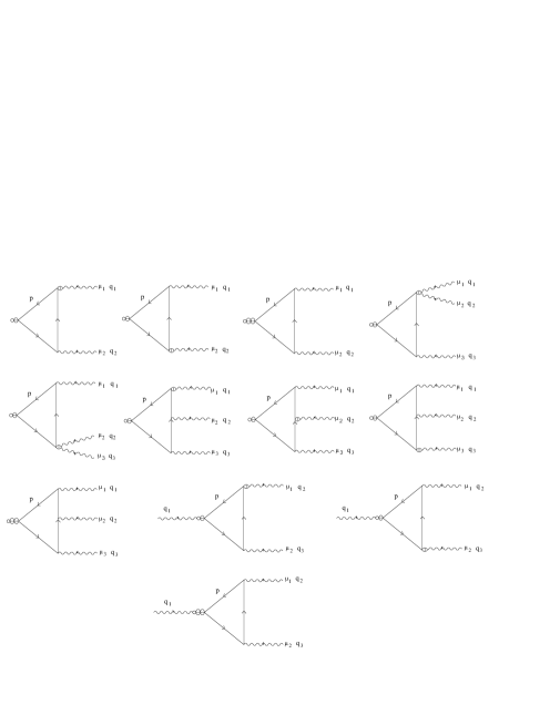
Fig. 4: Diagrams that yield ${\cal A}^{(cn)\,(2)}$ in eq. (3.84).

The computation of the Feynman diagrams in Fig. 4 with three gauge fields $a_{\mu}$ gives $\partial_{\beta}{\cal T}_{3}^{\beta}$. By performing that computation, we have obtained the following result:

$$\begin{array}[]{l}{\partial_{\beta}{\cal T}_{3}^{\beta}-\partial_{\beta}{\cal T}_{2}^{(inv)\,\beta}|_{aaa}={\partial}_{\beta}\Big{\{}i\frac{N_{f}}{96\pi^{2}}\theta^{\alpha\beta}\theta^{\rho\sigma}\epsilon^{{\mu_{1}}{\mu_{2}}{\mu_{3}}{\mu_{4}}}\text{Tr}\big{[}6\,{\partial}_{\alpha}\partial_{[\,\rho}a_{{\mu_{2}}]}\partial_{[\,\sigma}a_{{\mu_{3}}]}{\partial}_{\mu_{1}}a_{\mu_{4}}}\\ {\phantom{\partial_{\beta}{\cal T}_{3}^{\beta}}-6\,{\partial}_{\alpha}\partial_{[\,\rho}a_{{\mu_{2}}]}{\partial}_{\mu_{1}}a_{\mu_{3}}\partial_{[\,\sigma}a_{{\mu_{4}}]}+6\,{\partial}_{\alpha}{\partial}_{\mu_{1}}a_{\mu_{2}}\partial_{[\,\rho}a_{{\mu_{3}}]}\partial_{[\,\sigma}a_{{\mu_{4}}]}+7\,{\partial}_{\alpha}{\partial}_{\mu_{1}}a_{\mu_{3}}{\partial}_{\mu_{2}}a_{\mu_{4}}{\partial}_{\rho}a_{\sigma}}\\ {\phantom{\partial_{\beta}{\cal T}_{3}^{\beta}}+3\,{\partial}_{\rho}{\partial}_{\mu_{1}}a_{\mu_{3}}\partial_{[\,\sigma}a_{\alpha]}{\partial}_{\mu_{2}}a_{\mu_{4}}+5\,{\partial}_{\alpha}{\partial}_{\mu_{1}}a_{\mu_{3}}{\partial}_{\rho}a_{\sigma}{\partial}_{\mu_{2}}a_{\mu_{4}}+6\,{\partial}_{\alpha}{\partial}_{\rho}a_{\sigma}{\partial}_{\mu_{1}}a_{\mu_{3}}{\partial}_{\mu_{2}}a_{\mu_{4}}\big{]}}\\ {\phantom{\partial_{\beta}{\cal T}_{3}^{\beta}}-i\frac{N_{f}}{64\pi^{2}}\theta^{\alpha\beta}\theta^{\rho\sigma}\epsilon^{{\mu_{1}}{\mu_{2}}{\mu_{3}}{\mu_{4}}}\,g_{\alpha\rho}g^{\mu\nu}{\partial}_{\sigma}\text{Tr}\big{[}\partial_{\,[\mu}a_{{\mu_{2}}]}\partial_{\,[\nu}a_{{\mu_{3}}]}{\partial}_{\mu_{1}}a_{\mu_{4}}\big{]}\Big{\}}.}\\ \end{array}$$

Applying to the r.h.s. of the previous equation the replacements in eq. (3.67), one gets that

$$\begin{array}[]{l}{\partial_{\beta}{\cal T}_{3}^{(inv)\,\beta}={\partial}_{\beta}\Big{\{}i\frac{N_{f}}{96\pi^{2}}\theta^{\alpha\beta}\theta^{\rho\sigma}\epsilon^{{\mu_{1}}{\mu_{2}}{\mu_{3}}{\mu_{4}}}\text{Tr}\big{[}3\,{\mathfrak{D}}_{\alpha}f_{\rho{\mu_{2}}}f_{\sigma{\mu_{3}}}f_{{\mu_{1}}{\mu_{4}}}-3\,{\mathfrak{D}}_{\alpha}f_{\rho{\mu_{2}}}f_{{\mu_{1}}{\mu_{3}}}f_{\sigma{\mu_{4}}}}\\ {\phantom{\partial_{\beta}{\cal T}_{2}^{(inv)\,\beta}={\partial}_{\beta}\Big{\{}}+3\,{\mathfrak{D}}_{\alpha}f_{{\mu_{1}}{\mu_{2}}}f_{\rho{\mu_{3}}}f_{\sigma{\mu_{4}}}+\frac{7}{8}\,{\mathfrak{D}}_{\alpha}f_{{\mu_{1}}{\mu_{3}}}f_{{\mu_{2}}{\mu_{4}}}f_{\rho\sigma}+\frac{3}{4}\,{\mathfrak{D}}_{\rho}f_{{\mu_{1}}{\mu_{3}}}f_{\sigma\alpha}f_{{\mu_{2}}{\mu_{4}}}}\\ {+\frac{5}{8}\,{\mathfrak{D}}_{\alpha}f_{{\mu_{1}}{\mu_{3}}}f_{\rho\sigma}f_{{\mu_{2}}{\mu_{4}}}+\!\frac{3}{4}{\mathfrak{D}}_{\alpha}f_{\rho\sigma}f_{{\mu_{1}}{\mu_{3}}}f_{{\mu_{2}}{\mu_{4}}}\big{]}-\!i\frac{N_{f}}{128\pi^{2}}\theta^{\alpha\beta}\theta^{\rho\sigma}\epsilon^{{\mu_{1}}{\mu_{2}}{\mu_{3}}{\mu_{4}}}g_{\alpha\rho}g^{\mu\nu}{\partial}_{\sigma}\text{Tr}\big{[}f_{\mu{\mu_{2}}}f_{\nu{\mu_{3}}}f_{{\mu_{1}}{\mu_{4}}}\big{]}\Big{\}}.}\\ \end{array}$$ (3.89)

It is clear that $\partial_{\beta}{\cal T}_{3}^{(inv)\,\beta}$ verifies eq. (3.86).

Substituting eqs. (3.89) and (3.88) in eq (3.87), one obtains the following result:

$$\begin{array}[]{l}{{\cal A}^{(cn)\,(2)}={\partial}_{\beta}\Big{\{}-\frac{N_{f}}{384\pi^{2}}\,\theta^{\alpha\beta}\theta^{\rho\sigma}\epsilon^{{\mu_{1}}{\mu_{2}}{\mu_{3}}{\mu_{4}}}\,\big{(}\text{Tr}\,{\mathfrak{D}}_{\alpha}{\mathfrak{D}}_{\sigma}f_{{\mu_{1}}{\mu_{3}}}{\mathfrak{D}}_{\rho}f_{{\mu_{2}}{\mu_{4}}}+{\partial}_{\sigma}\text{Tr}\big{[}\frac{3}{2}{\mathfrak{D}}_{\alpha}f_{{\mu_{1}}{\mu_{3}}}{\mathfrak{D}}_{\rho}f_{{\mu_{2}}{\mu_{4}}}}\\ {\phantom{{\cal A}^{(cn)\,(2)}={\partial}_{\beta}\Big{\{}}+2{\mathfrak{D}}_{\rho}{\mathfrak{D}}_{\alpha}f_{{\mu_{1}}{\mu_{3}}}f_{{\mu_{2}}{\mu_{4}}}\big{]}\big{)}+\frac{N_{f}}{512\pi^{2}}\,\theta^{\alpha\beta}\theta^{\rho\sigma}\epsilon^{{\mu_{1}}{\mu_{2}}{\mu_{3}}{\mu_{4}}}g_{\alpha\rho}g^{\mu\nu}{\partial}_{\sigma}\text{Tr}\big{[}2\,{\mathfrak{D}}_{\mu}{\mathfrak{D}}_{\nu}f_{{\mu_{1}}{\mu_{3}}}f_{{\mu_{2}}{\mu_{4}}}}\\ {\phantom{{\cal A}^{(cn)\,(2)}={\partial}_{\beta}\Big{\{}}+{\mathfrak{D}}_{\mu}f_{{\mu_{1}}{\mu_{3}}}{\mathfrak{D}}_{\nu}f_{{\mu_{2}}{\mu_{4}}}\big{]}}\\ {\phantom{{\cal A}^{(cn)\,(2)}={\partial}_{\beta}\Big{\{}}+i\frac{N_{f}}{96\pi^{2}}\theta^{\alpha\beta}\theta^{\rho\sigma}\epsilon^{{\mu_{1}}{\mu_{2}}{\mu_{3}}{\mu_{4}}}\text{Tr}[3\,{\mathfrak{D}}_{\alpha}f_{\rho{\mu_{2}}}f_{\sigma{\mu_{3}}}f_{{\mu_{1}}{\mu_{4}}}-3\,{\mathfrak{D}}_{\alpha}f_{\rho{\mu_{2}}}f_{{\mu_{1}}{\mu_{3}}}f_{\sigma{\mu_{4}}}}\\ {\phantom{{\cal A}^{(cn)\,(2)}={\partial}_{\beta}\Big{\{}}+3\,{\mathfrak{D}}_{\alpha}f_{{\mu_{1}}{\mu_{2}}}f_{\rho{\mu_{3}}}f_{\sigma{\mu_{4}}}+\frac{7}{8}\,{\mathfrak{D}}_{\alpha}f_{{\mu_{1}}{\mu_{3}}}f_{{\mu_{2}}{\mu_{4}}}f_{\rho\sigma}+\frac{3}{4}\,{\mathfrak{D}}_{\rho}f_{{\mu_{1}}{\mu_{3}}}f_{\sigma\alpha}f_{{\mu_{2}}{\mu_{4}}}}\\ {\phantom{{\cal A}^{(cn)\,(2)}={\partial}_{\beta}\Big{\{}}+\frac{5}{8}\,{\mathfrak{D}}_{\alpha}f_{{\mu_{1}}{\mu_{3}}}f_{\rho\sigma}f_{{\mu_{2}}{\mu_{4}}}+\frac{3}{4}\,{\mathfrak{D}}_{\alpha}f_{\rho\sigma}f_{{\mu_{1}}{\mu_{3}}}f_{{\mu_{2}}{\mu_{4}}}\big{]}}\\ {\phantom{{\cal A}^{(cn)\,(2)}={\partial}_{\beta}\Big{\{}}-i\frac{N_{f}}{128\pi^{2}}\theta^{\alpha\beta}\theta^{\rho\sigma}\epsilon^{{\mu_{1}}{\mu_{2}}{\mu_{3}}{\mu_{4}}}\,g_{\alpha\rho}g^{\mu\nu}{\partial}_{\sigma}\text{Tr}f_{\mu{\mu_{2}}}f_{\nu{\mu_{3}}}f_{{\mu_{1}}{\mu_{4}}}\Big{\}}.}\\ \end{array}$$

Using linear equations that can be derived quite easily from eqs. (D.102) and (D.103), one may simplify the previous equation and obtain:

$${\cal A}^{(cn)\,(2)}=\partial_{\beta}{\cal Z}^{\beta},$$ (3.90)

where

$$\begin{array}[]{l}{{\cal Z}^{\beta}=+\frac{N_{f}}{1536\pi^{2}}\,\theta^{\alpha\beta}\theta^{\rho\sigma}\epsilon^{{\mu_{1}}{\mu_{2}}{\mu_{3}}{\mu_{4}}}\,\text{Tr}\,\big{[}2\,{\mathfrak{D}}_{\alpha}{\mathfrak{D}}_{\rho}f_{{\mu_{1}}{\mu_{3}}}{\mathfrak{D}}_{\sigma}f_{{\mu_{2}}{\mu_{4}}}+10\,i\,{\mathfrak{D}}_{\rho}f_{{\mu_{1}}{\mu_{3}}}f_{\sigma\alpha}f_{{\mu_{2}}{\mu_{4}}}}\\ {\phantom{{\cal Z}^{\beta}=+\frac{N_{f}}{1536\pi^{2}}\,\theta}+2\,i\,{\mathfrak{D}}_{\rho}f_{{\mu_{1}}{\mu_{3}}}f_{{\mu_{2}}{\mu_{4}}}f_{\sigma\alpha}+i{\mathfrak{D}}_{\alpha}f_{{\mu_{1}}{\mu_{2}}}f_{\rho\sigma}f_{{\mu_{3}}{\mu_{4}}}-i\,{\mathfrak{D}}_{\alpha}f_{{\mu_{1}}{\mu_{2}}}f_{{\mu_{3}}{\mu_{4}}}f_{\rho\sigma}\big{]}}\\ {\phantom{{\cal Z}^{\beta}=}+\frac{N_{f}}{512\pi^{2}}\,\theta^{\alpha\beta}\theta^{\rho\sigma}\epsilon^{{\mu_{1}}{\mu_{2}}{\mu_{3}}{\mu_{4}}}g_{\alpha\rho}g^{\mu\nu}\,\text{Tr}\,{\partial}_{\sigma}\big{[}2\,{\mathfrak{D}}_{\mu}{\mathfrak{D}}_{\nu}f_{{\mu_{1}}{\mu_{3}}}f_{{\mu_{2}}{\mu_{4}}}+{\mathfrak{D}}_{\mu}f_{{\mu_{1}}{\mu_{3}}}{\mathfrak{D}}_{\nu}f_{{\mu_{2}}{\mu_{4}}}}\\ {\phantom{{\cal Z}^{\beta}=+\frac{N_{f}}{1536\pi^{2}}\,\theta}-4\,i\,f_{\mu{\mu_{2}}}f_{\nu{\mu_{3}}}f_{{\mu_{1}}{\mu_{4}}}\big{]}.}\\ \end{array}$$ (3.91)

Finally, taking into account eqs (3.91), (3.90), (3.85), (3.84) and (3.81), one comes to the conclusion that

$$\partial_{\mu}<j_{5}^{(cn)\,\mu}(x)>^{(A)}_{MS}-\partial_{\mu}<j_{5}^{(np)\,\mu}(x)>^{(A)}_{MS}\,=\,h^{2}\,{\cal A}^{(cn)\,(2)}\neq 0.$$ (3.92)

Let $N[j_{5}^{(cn)\,\mu}]_{MS}(x)$ and $N[j_{5}^{(np)\,\mu}]_{MS}(x)$ be renormalized operators –called normal products [53, 55]– constructed by MS renormalization from the dimensionally regularized currents $j_{5}^{(cn)\,\mu}(x)$ and $j_{5}^{(np)\,\mu}(x)$, respectively. Then, the previous equation shows that the difference between $N[j_{5}^{(cn)\,\mu}]_{MS}(x)$ and $N[j_{5}^{(np)\,\mu}]_{MS}(x)$ is an operator, say $N[{\cal Y}^{\mu}]$, which does not verify $\partial_{\mu}N[{\cal Y}^{\mu}]_{MS}(x)=0$, even upon imposing the equations of motion. This is in contradiction to the classical case. And yet, as we shall see below, both currents, defined in terms of normal products, yield, if $\theta^{0i}=0$, the same chiral charge up to order $h^{2}$. But first, let us see that the $\theta^{\mu\nu}$-dependent contributions in eq. (3.92) are not anomalous contributions, but finite renormalizations of the current $N[j_{5}^{(cn)\,\mu}(x)]$. Indeed, eqs. (3.92) and (3.76) lead to

$$\partial_{\mu}N[j_{5}^{(cn)\;\mu}]_{MS}(x)\,=\,\frac{N_{f}}{8\pi^{2}}\text{Tr}\,f_{{\mu_{1}}{\mu_{2}}}(x)\tilde{f}_{{\mu_{3}}{\mu_{4}}}(x)\,+\,h^{2}\,\partial_{\lambda}\,{\cal X}^{\lambda}(x)\,+\,h^{2}\,\partial_{\beta}{\cal Z}^{\beta},$$

where ${\cal X}^{\lambda}(x)$ and ${\cal Z}^{\beta}$ are the gauge invariant vector fields in eqs. (3.74) and (3.91), respectively. Then, we introduce a new current, say ${\cal J}_{5}^{(cn)\,\mu}$, defined as follows

$${\cal J}_{5}^{(cn)\,\mu}(x)\,=\,N[j_{5}^{(cn)\;\mu}]_{MS}(x)\,-\,h^{2}\,{\cal X}^{\mu}(x)\,-\,h^{2}\,{\cal Z}^{\mu}(x).$$ (3.93)

This new current is to be understood as a finite renormalization of $N[j_{5}^{(cn)\;\mu}]_{MS}(x)$, and satisfies the ordinary $U(1)_{A}$ anomaly equation:

$$\partial_{\mu}{\cal J}_{5}^{(cn)\,\mu}(x)\,=\,\ \frac{N_{f}}{8\pi^{2}}\,\text{Tr}\,f_{{\mu_{1}}{\mu_{2}}}(x)\tilde{f}_{{\mu_{3}}{\mu_{4}}}(x).$$ (3.94)

It is plain that ${\cal X}^{0}=0={\cal Z}^{0}$, if $\theta^{0i}=0$. Hence, if time is commutative both ${\cal J}_{5}^{(cn)\,\mu}(x)$ and $N[j_{5}^{(cn)\;\mu}]_{MS}(x)$ give rise to the same chiral charge $Q_{5}^{(cn)}$. Integrating both sides of eq. (3.94) over all values of $x$, one concludes that, unlike its ordinary counterpart, the quantum $Q_{5}^{(cn)}$ is no longer conserved in the presence of topologically nontrivial field configurations:

$$Q_{5}^{(cn)}(t=+\infty)-Q_{5}^{(cn)}(t=-\infty)\,=\,\frac{N_{f}}{8\pi^{2}}\int\!d^{4}\!x\,\,\text{Tr}\,f_{{\mu_{1}}{\mu_{2}}}\tilde{f}_{{\mu_{3}}{\mu_{4}}}\,=\,2\,N_{f}\,(n_{+}-n_{-}).$$ (3.95)

The integers $n_{\pm}$ are defined in eq. (2.28). To obtain the result in the far right of the previous equation we have used the temporal gauge $a_{0}(x)=0$ and the boundary conditions in eq. (2.27). Again, eq. (3.95) is the spitting image of eq. (3.78). This is no wonder since, as we shall see next, the MS renormalized $Q_{5}^{(cn)}(t)$ and $Q_{5}^{(np)}(t)$ agree up to second order in $h$, at the least. Using the identities in eq. (3.79), one can show that the following equations hold for $\theta^{0i}=0$:

$$N[j_{5}^{(cn)\,0}]_{MS}-N[j_{5}^{(np)\,0}]_{MS}=\partial_{i}\,R^{i}.$$

$R^{i}$ denotes the operator

$$\begin{array}[]{l}{-i\frac{h}{2}\,\theta^{ij}N[\bar{\psi}\gamma^{0}\gamma_{5}D_{j}\psi]_{MS}+h^{2}\,\theta^{ij}\theta^{i^{\prime}j^{\prime}}\Big{[}+\frac{1}{8}\partial_{i^{\prime}}N[\bar{\psi}\gamma^{0}\gamma_{5}D_{j}D_{j^{\prime}}\psi]_{MS}\phantom{aaaaaaaaa}}\\ {\phantom{aaaaaaaaaaaaaaa}-\frac{1}{8}N[\bar{\psi}\gamma^{0}\gamma_{5}D_{i^{\prime}}\{D_{j^{\prime}},D_{j}\}\psi]_{MS}-\frac{1}{4}N[\bar{\psi}\gamma^{0}\gamma_{5}D_{j}D_{i^{\prime}}D_{j^{\prime}}\psi]_{MS}\phantom{aaaaaaaaa}}\\ {\phantom{aaaaaaaaaaaaaaaaaaaaaa}+\frac{1}{4}N[\bar{\psi}\gamma^{o}\gamma_{5}D_{i^{\prime}}D_{j}D_{j^{\prime}}\psi]_{MS}\,\Big{]}+o(h^{3}).}\\ \end{array}$$

Then,

$$Q_{5}^{(cn)}=\int d^{3}\vec{x}\;N[j_{5}^{(cn)\,0}]_{MS}=\int d^{3}\vec{x}\;N[j_{5}^{(np)\,0}]_{MS}+\int d^{3}\vec{x}\;\partial_{i}\,R^{i}=Q_{5}^{(np)}\,+\,o(h^{3}).$$

We have assumed that the fields go sufficiently rapidly to zero at spatial infinity so that the last integral vanishes.

4 Nonsinglet chiral currents are anomaly free

The $SU(N_{f})_{A}$ canonical Noether current, i.e., the canonical nonsinglet chiral current, reads

$$j_{5}^{(cn)\,a\mu}\,=\,\sum_{ff^{\prime}}\bar{\psi}_{f}\,{\cal H}\,T^{a}_{ff^{\prime}}\psi_{f^{\prime}}.$$

Where ${\cal H}$ is the object that is left after removing from $j^{\mu}_{(cn)}$ in eq. (2.10) the fields $\bar{\psi}_{f}$ and $\psi_{f}$. We also have the nonsinglet current, $j_{5}^{(np)\,a\mu}$, which is the analog of the singlet current $j_{5}^{(np)\,\mu}$ in eq. (2.14):

$$j_{5}^{(np)\,a\mu}=\sum_{ff^{\prime}}\bar{\Psi}_{f}T^{a}_{ff^{\prime}}\gamma_{5}\star\Psi_{f^{\prime}}.$$

These two nonsinglet currents are divergenceless classically since the classical theory has the $SU(N_{f})_{A}$ symmetry in eq. (2.8). The dimensionally regularized currents constructed from $j_{5}^{(cn)\,a\mu}$ and $j_{5}^{(np)\,a\mu}$ above verify the following equations

$$\begin{array}[]{l}{\partial_{\mu}<j_{5}^{(cn)\,a\mu}>^{(A)}=\partial_{\mu}<j_{5}^{(np)\,a\mu}>^{(A)}\,+\,\partial_{\mu}\hat{{\cal X}}^{a\,\mu}_{(ns)}},\\ {\partial_{\mu}<j_{5}^{(np)\,a\mu}>^{(A)}=2\,\sum_{ff^{\prime}}\,<\bar{\Psi}_{f}\star T^{a}_{ff^{\prime}}{\hat{\gamma}}^{a\,\mu}\gamma_{5}\Psi_{f^{\prime}}>^{(A)}.}\\ \end{array}$$ (4.96)

Here, $\hat{{\cal X}}^{a\,\mu}_{(ns)}=\sum_{ff^{\prime}}\bar{\psi}_{f}\,{\cal K}\,T^{a}_{ff^{\prime}}\psi_{f^{\prime}}$. ${\cal K}$ is obtained by stripping $\bar{\psi}_{f}$ and $\psi_{f}$ off the r.h.s. of eq. (3.83). Now, since the kinetic terms and vertices of our noncommutative theory are in flavour space proportional to the identity, it is clear that the contributions to the r.h.s. of the equalities in eq. (4.96) can be obtained from the corresponding singlet contributions by multiplying them by $\text{Tr}\,T^{a}$ –see eqs. (3.56), (3.60), (3.73), (3.74) and (3.83), and diagrams in Figs. 1, 2 and 3. But, $\text{Tr}\,T^{a}=0$, so that

$$\partial_{\mu}<j_{5}^{(cn)\,a\mu}>^{(A)}=0,\qquad\partial_{\mu}<j_{5}^{(np)\,a\mu}>^{(A)}=0.$$

We have thus shown that, at least at the one-loop level and second order in $h$, the quantum nonsinglet currents of the $SU(N_{f})_{A}$ classical symmetry of the theory are anomaly free.

5 Summary and conclusions

In this paper we have obtained, at the one-loop level and second order in $\theta^{\mu\nu}$, the anomaly equation for the canonical Noether current –$j_{5}^{(cn)\,\mu}$ in eq. (2.10)– of the classical $U(1)_{A}$ symmetry of noncommutative $SU(N)$ gauge theory with massless fermions. All along this paper the physical $\theta^{\mu\nu}$ has been considered to be of “magnetic” type: $\theta^{i0}=0$. We have shown that the current $j_{5}^{(cn)\,\mu}$ can be renormalized to a current –${\cal J}_{5}^{(cn)\,\mu}$ in eq. (3.93)– such that the anomalous contribution to the fourdivergence of the latter is just the ordinary anomaly. This is a highly nontrivial result since, a priori, there are $\theta^{\mu\nu}-$dependent candidates to the $U(1)_{A}$ anomaly such as

$$\theta^{\rho\sigma}\epsilon^{\mu_{1}\mu_{2}\mu_{3}\mu_{4}}\text{Tr}\,[f_{\sigma\mu_{1}}f_{\mu_{2}\mu_{3}}f_{\rho\mu_{4}}],\quad\theta^{\alpha\beta}\theta^{\rho\sigma}\,\epsilon^{{\mu_{1}}{\mu_{2}}{\mu_{3}}{\mu_{4}}}\,\text{Tr}\,\Big{[}f_{{\mu_{1}}{\mu_{2}}}f_{{\mu_{3}}{\mu_{4}}}f_{\alpha\rho}f_{\beta\sigma}\Big{]},\quad{\it etc}...$$

We have shown that all these would-be anomalous contributions neatly cancel among themselves –see eqs. (3.60), (3.71) and (3.72). We have also studied the anomaly equation for other noncommutative currents that are classically (covariantly) conserved as a consequence of the $U(1)_{A}$ invariance of the classical action. These currents go under the names of $j_{5}^{(p)\,\mu}$ and $j_{5}^{(np)\,\mu}$ and their (covariant) fourdivergences in the MS scheme are given in eqs. (3.44) and (3.76). Classically, the current $j_{5}^{(np)\,\mu}$ is also a Noether current, for it is related with the canonical Noether current $j_{5}^{(cn)\,\mu}$ by eq. (2.26) –see also eq. (2.12)–. This relationship does not hold for the MS renormalized currents. However, at the one-loop level, we have been able to introduce a current –${\cal J}_{5}^{(np)\,\mu}$ in eq. (3.77)– which is obtained by nonminimal renormalization of $j_{5}^{(np)\,\mu}$ and whose difference with ${\cal J}_{5}^{(cn)\,\mu}$ is a certain ${\cal Y}^{\mu}$ satisfying the criteria in eq. (2.13).

We have also shown that, at least up to second order in $\theta^{\mu\nu}$, all the $U(1)_{A}$ currents considered above yield the same chiral charge, say $Q^{(cn)}_{5}(t)$, if $\theta^{0i}=0$. Of course, this classically conserved charge is not conserved at the quantum level, but verifies the following equation:

$$Q^{(cn)}_{5}(t=+\infty)-Q^{(cn)}_{5}(t=-\infty)\,=\,\frac{N_{f}}{8\pi^{2}}\int\!d^{4}\!x\,\,\text{Tr}\,f_{{\mu_{1}}{\mu_{2}}}\tilde{f}_{{\mu_{3}}{\mu_{4}}}\,=\,2\,N_{f}\,(n_{+}-n_{-}).$$ (5.97)

To obtain the result in the far right of the previous equation, the temporal gauge, $a_{o}(x)=0$, has been used and the boundary conditions in eq. (2.27) have been imposed. The integers $n_{\pm}$ are defined in eq. (2.28). The identity on the far right of eq. (2.29) puts us in the position of giving to eq. (5.97) a clear physical meaning. What eq. (5.97) shows is that in any quantum transition from $t=-\infty$ to $t=+\infty$ that involve a change in the topological properties of the asymptotic gauge fields –i.e., $n_{+}-n_{-}=n\neq 0$–, there is, for $(n<0)n>0$, a transmutation of the (right-) left-handed fermionic degrees of freedom at $t=-\infty$ into (left-) right-handed degrees at $t=\infty$. For instance, take $n>0$, then, if in that transition the fermionic part of the physical state at $t=-\infty$ is constituted by $nN_{f}$ left-handed fermions, then, the fermionic part of the physical state at $t=+\infty$ will be made of $nN_{f}$ right-handed fermions. Of course, there will be “compulsory” creation of fermion-antifermion pairs at $t=+\infty$, if there are no fermionic degrees of freedom at $t=-\infty$. It is well known that these phenomena also occur in ordinary space-time, so introducing noncommutative space-time does not change the qualitative picture; it does change, however, the quantitative analysis of these phenomena. For instance, upon Wick rotation the dominant contribution to the path integral coming from the gauge fields is a certain $\theta^{\mu\nu}-$deformation of the ordinary BPST instanton. This deformation, in turn, gives rise to a $\theta^{\mu\nu}-$dependent effective ’t Hooft vertex. We shall report on these findings elsewhere [59].

Next, taking into account that we have shown that $Q^{(cn)}_{5}(t)=Q^{(pn)}_{5}(t)=Q^{(p)}_{5}(t)$ is verified at least up to second order in $\theta^{\mu\nu}$ and the fact that eq. (3.46) is valid at the one-loop level and any order in $\theta^{\mu\nu}$, it is not foolish to conjecture that eq. (5.97) will hold at any order in $\theta^{\mu\nu}$.

Now, since in our computations the actual properties of $T^{a}$ –the generators of $SU(N)$– have played no role, barring its hermiticity and the cyclicity of trace of any product of them, we conclude that all our expressions are valid for $SO(N)$ groups. Our expressions are also valid for $U(1)$ provided we replace $a_{\mu}$ with $Q\,a_{\mu}$. $Q$ being the charge of the fermion coupled to the $U(1)$ field $a_{\mu}$.

Finally, it is quite obvious how to generalize our expressions to encompass the situation where several representations –labeled by R– of the gauge group are at work in the fermionic action. Let us give just one instance. Assume that we have $N^{({\cal R})}_{f}$ fermions which couple to the gauge field, $a^{({\cal R})}_{\mu}$, in the ${\cal R}$ representation of the gauge group. Then, eq. (3.94) will read:

$$\partial_{\mu}{\cal J}_{5}^{(cn)\,\mu}(x)\,=\,\ \sum_{{\cal R}}\frac{N^{({\cal R})}_{f}}{8\pi^{2}}\,\text{Tr}\,f^{({\cal R})}_{{\mu_{1}}{\mu_{2}}}(x)\tilde{f}^{({\cal R})}_{{\mu_{3}}{\mu_{4}}}(x),$$

with

$${\cal J}_{5}^{(cn)\,\mu}(x)\,=\,\sum_{{\cal R}}\,N[j_{5}^{({\cal R})\,(cn)\;\mu}]_{MS}(x)\,-\,h^{2}\,\sum_{{\cal R}}\,{\cal X}^{({\cal R})\,\mu}(x)\,-\,h^{2}\,\sum_{{\cal R}}\,{\cal Z}^{({\cal R})\,\mu}(x).$$

The gauge fields in $j_{5}^{({\cal R})\,(cn)\;\mu}$, ${\cal X}^{({\cal R})\,\mu}$ and ${\cal Z}^{({\cal R})\,\mu}$ are all in the ${\cal R}$ representation of the gauge group.

6 Acknowledgments

We thank L. Moeller for fruitful correspondence. This work has been financially supported in part by MEC through grant BFM2002-00950. The work of C. Tamarit has also received financial support from MEC trough FPU grant AP2003-4034.

Appendix A

In this Appendix we give the Feynman rules needed to turn into mathematical objects the Feynman diagrams displayed in this paper. These Feynman rules are in Fig. 5.

Appendix B

In this Appendix we display some equalities verified by the “$D$-dimensional” Lorentz covariants introduced in ref. [52], which are used in our computations.

$$\begin{array}[]{l}{\,\,\phantom{\hat{g}}g^{\mu\nu}\hat{g}_{\nu\rho}=\hat{g}^{\mu}_{\rho},\quad\quad\quad\quad\quad\quad\quad\quad\quad\hat{g}^{\mu}_{\mu}=2\epsilon,\quad\quad\quad\quad\quad\quad\quad\quad\epsilon^{\mu\nu\rho\sigma}\hat{g}_{\sigma\eta}=0,}\\ {\{\gamma^{\mu},\gamma^{\nu}\}=2\gamma^{\mu\nu}\mathbb{I},\quad\quad\quad\{\gamma_{5},\gamma^{\mu}\}=\{\gamma_{5},\hat{\gamma}^{\mu}\}=2\gamma_{5}\hat{\gamma}^{\mu},\quad\quad\quad\quad\,[\gamma_{5},\hat{\gamma}^{\mu}]\,=\,0.}\\ \end{array}$$ (B.98)

$$\begin{array}[]{l}{\text{tr}\gamma_{5}\hat{\gamma}^{\mu_{1}}\gamma^{\mu_{2}}\dots\gamma^{\mu_{2}k}=}\\ {\frac{1}{2}\left[\text{tr}\gamma_{5}\{\hat{\gamma}^{\mu_{1}},\gamma^{\mu_{2}}\}\gamma^{\mu_{3}}\dots\gamma^{\mu_{2k}}+\text{tr}\gamma_{5}\gamma^{\mu_{2}}\left\{\hat{\gamma}^{\mu_{1}},\gamma^{\mu_{3}}\right\}\dots\gamma^{\mu_{2k}}+\dots+\text{tr}\gamma_{5}\gamma^{\mu_{2}}\dots\{\hat{\gamma}^{\mu_{1}},\gamma^{\mu_{2}}\}\right].}\end{array}$$ (B.99)

$$\text{tr}\,\gamma_{5}\gamma^{\mu_{1}}\gamma^{\mu_{2}}\,=\,0,\quad\quad\text{tr}\,\gamma_{5}\gamma^{\mu_{1}}\gamma^{\mu_{2}}\gamma^{\mu_{3}}\,=\,0,\quad\quad\text{tr}\,\gamma_{5}\gamma^{\mu_{1}}\dots\gamma^{\mu_{4}}\,=\,i\;\text{tr}\,\mathbb{I}\;\epsilon^{\mu_{1}\dots\mu_{4}}.$$

$$\text{tr}\,\gamma_{5}\gamma^{\mu_{1}}\dots\gamma^{\mu_{6}}\,=\,\;\text{tr}\,\mathbb{I}\;\sum_{p<q}{(-1)^{q-p}\epsilon^{\mu_{1}\dots\mu_{p-1}\mu_{p+1}\dots\mu_{q-1}\mu_{q+1}\dots\mu_{6}}}\,g^{\mu_{p}\mu_{q}}.$$

Appendix C

Here we include the list of the dimensionally regularized integrals that are need to work out the would-be anomalous contributions. The dimensional regularization regulator $\epsilon$ is equal to $\frac{D-4}{2}$. Contributions that vanish as $\epsilon\rightarrow 0$ are never included. The symbol “$\sim$” shows that we have dropped contributions of the type $\frac{1}{\epsilon}\hat{O}$, where $\hat{O}$ is an evanescent tensor, for they are not actually needed: they are subtracted by the renormalization algorithm.

$$\begin{array}[]{l}{\int\!\frac{d^{D}\!p}{(2\pi)^{D}}\,\,\frac{\hat{p}^{2}}{(p-a)^{2}(p-b)^{2}(p-c)^{2}}=\int\!\frac{d^{D}\!p}{(2\pi)^{D}}\,\,\frac{\hat{p}^{2}p^{2}}{(p-a)^{2}(p-b)^{2}(p-c)^{2}(p-d)^{2}}=\frac{-i}{32\pi^{2}},}\\ {\int\!\frac{d^{D}\!p}{(2\pi)^{D}}\,\,\frac{\hat{p}_{\alpha}p_{\beta}}{p^{2}(p-a)^{2}(p-b)^{2}}=\frac{-i}{64\pi^{2}\epsilon}\hat{g}_{\alpha\beta},}\\ {\int\!\frac{d^{D}\!p}{(2\pi)^{D}}\,\,\frac{\hat{p}^{2}p_{\alpha}p_{\beta}}{(p-a)^{2}(p-b)^{2}(p-c)^{2}(p-d)^{2}}=\frac{-i}{4!8\pi^{2}}\Big{\{}g_{\alpha\beta}+\frac{1}{\epsilon}\hat{g}_{\alpha\beta}\Big{\}},}\\ {\int\!\frac{d^{D}\!p}{(2\pi)^{D}}\,\,\frac{\hat{p}^{2}p^{2}p_{\alpha}}{(p-a)^{2}(p-b)^{2}(p-c)^{2}(p-d)^{2}}=\frac{-i}{6(4\pi)^{2}}\Big{\{}(a+\dots+d)_{\alpha}+\frac{1}{\epsilon}\,\hat{g}^{\nu}_{\alpha}(a+\dots+d)_{\nu}\Big{\}},}\\ {\int\!\frac{d^{D}\!p}{(2\pi)^{D}}\,\,\frac{\hat{p}^{2}p^{2}p_{\alpha}p_{\beta}}{(p-a)^{2}(p-b)^{2}(p-c)^{2}(p-d)^{2}(p-e)^{2}}=\frac{-i}{4!8\pi^{2}}\Big{\{}g_{\alpha\beta}+\frac{1}{\epsilon}\hat{g}_{\alpha\beta}\Big{\}},}\\ {\int\!\frac{d^{D}\!p}{(2\pi)^{D}}\,\,\frac{\hat{p}^{2}p_{\alpha}p_{\beta}}{(p-a)^{2}(p-b)^{2}(p-c)^{2}}=-\frac{i}{2(4\pi)^{2}}\Big{\{}2\Delta_{\alpha\beta}+\frac{4}{\epsilon}\hat{\Delta}_{\alpha\beta}+\frac{1}{\epsilon}g_{\alpha\beta}\hat{\Delta}^{\mu}_{\mu}\Big{\}}}\\ {\hskip 85.35826pt+\frac{i}{24(4\pi)^{2}}(a^{2}+b^{2}+c^{2}-a\cdot b-a\cdot c-b\cdot c)\Big{\{}g_{\alpha\beta}+\frac{1}{\epsilon}\hat{g}_{\alpha\beta}\Big{\}},}\\ {\hskip 85.35826pt\Delta_{\alpha\beta}\equiv\frac{1}{12}(a_{\alpha}a_{\beta}+b_{\alpha}b_{\beta}+c_{\alpha}c_{\beta})+\frac{1}{24}(a_{\alpha}b_{\beta}+a_{\alpha}c_{\beta}+b_{\alpha}c_{\beta}+\alpha\leftrightarrow\beta),}\\ {\int\!\frac{d^{D}\!p}{(2\pi)^{D}}\,\,\frac{\hat{p}^{2}p_{\alpha}p_{\beta}p_{\rho}}{(p-a)^{2}(p-b)^{2}(p-c)^{2}(p-d)^{2}}\sim}\\ {\hskip 56.9055pt\sim\frac{-i}{4!32\pi^{2}}\Big{\{}g_{\alpha\beta}(a+b+c+d)_{\rho}+g_{\alpha\rho}(a+b+c+d)_{\beta}+g_{\beta\rho}(a+b+c+d)_{\alpha}\Big{\}},}\\ \end{array}$$

$$\begin{array}[]{l}{\int\!\frac{d^{D}\!p}{(2\pi)^{D}}\,\,\frac{\hat{p}^{2}p^{2}p_{\alpha}p_{\beta}}{(p-a)^{2}(p-b)^{2}(p-c)^{2}(p-d)^{2}}\sim}\\ {\sim\frac{i}{384\pi^{2}}\,g_{\alpha\beta}\Big{\{}a^{2}+b^{2}+c^{2}+d^{2}-a\cdot(b+c+d)-b\cdot(c+d)-c\cdot d\Big{\}},}\\ {-\frac{i}{384\pi^{2}}\Big{\{}2a_{\alpha}a_{\beta}+2b_{\alpha}b_{\beta}+2c_{\alpha}c_{\beta}+2d_{\alpha}d_{\beta}+\big{[}a_{\alpha}(b+c+d)_{\beta}+b_{\alpha}(c+d)_{\beta}+c_{\alpha}d_{\beta}+\alpha\leftrightarrow\beta\big{]}\Big{\}},}\\ {\int\!\frac{d^{D}\!p}{(2\pi)^{D}}\,\,\frac{\hat{p}^{2}p_{\alpha}p_{\beta}p_{\rho}p_{\sigma}}{p^{2}(p-a)^{2}(p-b)^{2}(p-c)^{2}(p-d)^{2}}\sim\frac{-i}{1536\pi^{2}}\Big{\{}g_{\alpha\beta}g_{\rho\sigma}+g_{\alpha\rho}g_{\beta\sigma}+g_{\alpha\sigma}g_{\beta\rho}\Big{\}}.}\\ \end{array}$$

Appendix D

In this Appendix we shall work out a number of identities among the terms on the r.h.s of eq. (3.71) and explain how to use them to obtain our final answer for ${\cal A}^{(2)}$ given in eq. (3.72).

Let $t_{\mu_{1}\mu_{2}\cdots\mu_{n}}$ be an object with indices $\mu_{i}$, $i=1\cdots n$, where $\mu_{i}=0,1,2,3$ $\forall i$ and $n>4$. Then, if $[\mu_{1}\mu_{2}\cdots\mu_{n}]$ stands for antisymetrization of the indices, we have

$$t_{[\mu_{1}\mu_{2}\cdots\mu_{n}]}\,=\,0.$$

Taking into account the previous identity, the cyclicity of Tr and the antisymmetry properties of $\epsilon^{\mu_{1}\mu_{2}\mu_{3}\mu_{4}}$, one obtains the collection of beautiful identities displayed below:

$$\theta^{\rho\sigma}\epsilon^{\mu_{1}\mu_{2}\mu_{3}\mu_{4}}\,\text{Tr}\,f_{\sigma[\mu_{1}}f_{\mu_{2}\mu_{3}}f_{\mu_{4}\rho]}=0\Rightarrow\theta^{\rho\sigma}\epsilon^{\mu_{1}\mu_{2}\mu_{3}\mu_{4}}\,\text{Tr}\,\big{[}f_{\sigma\mu_{1}}f_{\mu_{2}\mu_{3}}f_{\rho\mu_{4}}-\frac{1}{4}f_{\mu_{1}\mu_{2}}f_{\mu_{3}\mu_{4}}f_{\sigma\rho}\big{]}=0.$$ (D.100)

$$\begin{array}[]{l}{\epsilon^{{\mu_{1}}{\mu_{2}}{\mu_{3}}{\mu_{4}}}\,\text{Tr}\,{{\mathfrak{D}}}_{\alpha}f_{\rho[\sigma}{{\mathfrak{D}}}_{\beta}f_{{\mu_{1}}{\mu_{2}}}f_{{\mu_{3}}{\mu_{4}}]}=0\Rightarrow}\\ {\phantom{\epsilon^{{\mu_{1}}{\mu_{2}}{\mu_{3}}{\mu_{4}}}}\epsilon^{{\mu_{1}}{\mu_{2}}{\mu_{3}}{\mu_{4}}}\,\text{Tr}\,[{{\mathfrak{D}}}_{\alpha}f_{\rho\sigma}{{\mathfrak{D}}}_{\beta}f_{{\mu_{1}}{\mu_{2}}}f_{{\mu_{3}}{\mu_{4}}}+2{{\mathfrak{D}}}_{\alpha}f_{\rho{\mu_{1}}}{{\mathfrak{D}}}_{\beta}f_{{\mu_{2}}{\mu_{3}}}f_{{\mu_{4}}\sigma}+2{{\mathfrak{D}}}_{\alpha}f_{\rho{\mu_{3}}}{{\mathfrak{D}}}_{\beta}f_{{\mu_{4}}\sigma}f_{{\mu_{1}}{\mu_{2}}}]=0,}\\ {\epsilon^{{\mu_{1}}{\mu_{2}}{\mu_{3}}{\mu_{4}}}\,\text{Tr}\,{{\mathfrak{D}}}_{\alpha}f_{[\rho{\mu_{1}}}{{\mathfrak{D}}}_{\beta}f_{{\mu_{2}}{\mu_{3}}}f_{{\mu_{4}}]\sigma}=0\Rightarrow}\\ {\phantom{\epsilon^{{\mu_{1}}{\mu_{2}}{\mu_{3}}{\mu_{4}}}}\epsilon^{{\mu_{1}}{\mu_{2}}{\mu_{3}}{\mu_{4}}}\,\text{Tr}\,[2{{\mathfrak{D}}}_{\alpha}f_{\rho{\mu_{1}}}{{\mathfrak{D}}}_{\beta}f_{{\mu_{2}}{\mu_{3}}}f_{{\mu_{4}}\sigma}+2{{\mathfrak{D}}}_{\alpha}f_{{\mu_{2}}{\mu_{3}}}{{\mathfrak{D}}}_{\beta}f_{{\mu_{4}}\rho}f_{{\mu_{1}}\sigma}+{{\mathfrak{D}}}_{\alpha}f_{{\mu_{1}}{\mu_{2}}}{{\mathfrak{D}}}_{\beta}f_{{\mu_{3}}{\mu_{4}}}f_{\rho\sigma}]=0,}\\ {\epsilon^{{\mu_{1}}{\mu_{2}}{\mu_{3}}{\mu_{4}}}\,\text{Tr}\,{{\mathfrak{D}}}_{\alpha}f_{[\sigma{\mu_{1}}}{{\mathfrak{D}}}_{\beta}f_{|\rho|{\mu_{2}}}f_{{\mu_{3}}{\mu_{4}}]}=0\Rightarrow}\\ {\phantom{\epsilon^{{\mu_{1}}{\mu_{2}}{\mu_{3}}{\mu_{4}}}}\epsilon^{{\mu_{1}}{\mu_{2}}{\mu_{3}}{\mu_{4}}}\,\text{Tr}\,[2{{\mathfrak{D}}}_{\alpha}f_{\sigma{\mu_{1}}}{{\mathfrak{D}}}_{\beta}f_{\rho{\mu_{2}}}f_{{\mu_{3}}{\mu_{4}}}+2{{\mathfrak{D}}}_{\alpha}f_{{\mu_{2}}{\mu_{3}}}{{\mathfrak{D}}}_{\beta}f_{\rho{\mu_{4}}}f_{\sigma{\mu_{1}}}+{{\mathfrak{D}}}_{\alpha}f_{{\mu_{3}}{\mu_{4}}}{{\mathfrak{D}}}_{\beta}f_{\rho\sigma}f_{{\mu_{1}}{\mu_{2}}}]=0.}\\ \end{array}$$ (D.101)

$$\begin{array}[]{l}{\epsilon^{{\mu_{1}}{\mu_{2}}{\mu_{3}}{\mu_{4}}}\,\text{Tr}\,f_{\alpha\beta}f_{\rho[\sigma}f_{{\mu_{1}}{\mu_{2}}}f_{{\mu_{3}}{\mu_{4}}]}=0\Rightarrow}\\ {\phantom{\epsilon^{{\mu_{1}}{\mu_{2}}{\mu_{3}}{\mu_{4}}}}\epsilon^{{\mu_{1}}{\mu_{2}}{\mu_{3}}{\mu_{4}}}\,\text{Tr}\,[f_{\alpha\beta}f_{\rho\sigma}f_{{\mu_{1}}{\mu_{2}}}f_{{\mu_{3}}{\mu_{4}}}+2f_{\alpha\beta}f_{\rho{\mu_{1}}}f_{{\mu_{2}}{\mu_{3}}}f_{{\mu_{4}}\sigma}+2f_{\alpha\beta}f_{\rho{\mu_{3}}}f_{{\mu_{4}}\sigma}f_{{\mu_{1}}{\mu_{2}}}]=0,}\\ {\epsilon^{{\mu_{1}}{\mu_{2}}{\mu_{3}}{\mu_{4}}}\,\text{Tr}\,f_{\rho\alpha}f_{\beta[\sigma}f_{{\mu_{1}}{\mu_{2}}}f_{{\mu_{3}}{\mu_{4}}]}=0\Rightarrow}\\ {\phantom{\epsilon^{{\mu_{1}}{\mu_{2}}{\mu_{3}}{\mu_{4}}}}\epsilon^{{\mu_{1}}{\mu_{2}}{\mu_{3}}{\mu_{4}}}\,\text{Tr}\,[f_{\rho\alpha}f_{\beta\sigma}f_{{\mu_{1}}{\mu_{2}}}f_{{\mu_{3}}{\mu_{4}}}+2f_{\rho\alpha}f_{\beta{\mu_{1}}}f_{{\mu_{2}}{\mu_{3}}}f_{{\mu_{4}}\sigma}+2f_{\rho\alpha}f_{\beta{\mu_{3}}}f_{{\mu_{4}}\sigma}f_{{\mu_{1}}{\mu_{2}}}]=0,}\\ {\epsilon^{{\mu_{1}}{\mu_{2}}{\mu_{3}}{\mu_{4}}}\,\text{Tr}\,f_{\rho[\sigma}f_{|\alpha\beta|}f_{{\mu_{1}}{\mu_{2}}}f_{{\mu_{3}}{\mu_{4}}]}=0\Rightarrow}\\ {\phantom{\epsilon^{{\mu_{1}}{\mu_{2}}{\mu_{3}}{\mu_{4}}}}\epsilon^{{\mu_{1}}{\mu_{2}}{\mu_{3}}{\mu_{4}}}\,\text{Tr}\,[f_{\rho\sigma}f_{\alpha\beta}f_{{\mu_{1}}{\mu_{2}}}f_{{\mu_{3}}{\mu_{4}}}+2f_{\rho{\mu_{1}}}f_{\alpha\beta}f_{{\mu_{2}}{\mu_{3}}}f_{{\mu_{4}}\sigma}+2f_{\rho{\mu_{3}}}f_{\alpha\beta}f_{{\mu_{4}}\sigma}f_{{\mu_{1}}{\mu_{2}}}]=0.}\\ \end{array}$$ (D.102)

$$\begin{array}[]{l}{\epsilon^{{\mu_{1}}{\mu_{2}}{\mu_{3}}{\mu_{4}}}\,\text{Tr}\,f_{\alpha\beta}f_{[\sigma{\mu_{1}}}f_{|\rho|{\mu_{2}}}f_{{\mu_{3}}{\mu_{4}}]}=0\Rightarrow}\\ {\phantom{\epsilon^{{\mu_{1}}{\mu_{2}}{\mu_{3}}{\mu_{4}}}}\epsilon^{{\mu_{1}}{\mu_{2}}{\mu_{3}}{\mu_{4}}}\,\text{Tr}\,[2f_{\alpha\beta}f_{\sigma{\mu_{1}}}f_{\rho{\mu_{2}}}f_{{\mu_{3}}{\mu_{4}}}+2f_{\alpha\beta}f_{{\mu_{1}}{\mu_{2}}}f_{\rho{\mu_{3}}}f_{{\mu_{4}}\sigma}+f_{\alpha\beta}f_{{\mu_{3}}{\mu_{4}}}f_{\rho\sigma}f_{{\mu_{1}}{\mu_{2}}}]=0,}\\ {\epsilon^{{\mu_{1}}{\mu_{2}}{\mu_{3}}{\mu_{4}}}\,\text{Tr}\,f_{\alpha[\sigma}f_{|\beta\rho|}f_{{\mu_{1}}{\mu_{2}}}f_{{\mu_{3}}{\mu_{4}}]}=0\Rightarrow}\\ {\phantom{\epsilon^{{\mu_{1}}{\mu_{2}}{\mu_{3}}{\mu_{4}}}}\epsilon^{{\mu_{1}}{\mu_{2}}{\mu_{3}}{\mu_{4}}}\,\text{Tr}\,[f_{\alpha\sigma}f_{\beta\rho}f_{{\mu_{1}}{\mu_{2}}}f_{{\mu_{3}}{\mu_{4}}}+2f_{\alpha{\mu_{1}}}f_{\beta\rho}f_{{\mu_{2}}{\mu_{3}}}f_{{\mu_{4}}\sigma}+2f_{\alpha{\mu_{3}}}f_{\beta\rho}f_{{\mu_{4}}\sigma}f_{{\mu_{1}}{\mu_{2}}}]=0,}\\ {\epsilon^{{\mu_{1}}{\mu_{2}}{\mu_{3}}{\mu_{4}}}\,\text{Tr}\,f_{\rho\alpha}f_{[\sigma{\mu_{1}}}f_{|\beta|{\mu_{2}}}f_{{\mu_{3}}{\mu_{4}}]}=0\Rightarrow}\\ {\phantom{\epsilon^{{\mu_{1}}{\mu_{2}}{\mu_{3}}{\mu_{4}}}}\epsilon^{{\mu_{1}}{\mu_{2}}{\mu_{3}}{\mu_{4}}}\,\text{Tr}\,[2f_{\rho\alpha}f_{\sigma{\mu_{1}}}f_{\beta{\mu_{2}}}f_{{\mu_{3}}{\mu_{4}}}+2f_{\rho\alpha}f_{{\mu_{1}}{\mu_{2}}}f_{\beta{\mu_{3}}}f_{{\mu_{4}}\sigma}+2f_{\rho\alpha}f_{{\mu_{3}}{\mu_{4}}}f_{\beta\sigma}f_{{\mu_{1}}{\mu_{2}}}]=0,}\\ {\epsilon^{{\mu_{1}}{\mu_{2}}{\mu_{3}}{\mu_{4}}}\,\text{Tr}\,f_{\rho[\sigma}f_{|\alpha|{\mu_{1}}}f_{|\beta|{\mu_{2}}}f_{{\mu_{3}}{\mu_{4}}]}=0\Rightarrow}\\ {\phantom{\epsilon^{{\mu_{1}}{\mu_{2}}{\mu_{3}}{\mu_{4}}}}\epsilon^{{\mu_{1}}{\mu_{2}}{\mu_{3}}{\mu_{4}}}\,\text{Tr}\,[f_{\rho\sigma}f_{\alpha{\mu_{1}}}f_{\beta{\mu_{2}}}f_{{\mu_{3}}{\mu_{4}}}+2f_{\rho{\mu_{1}}}f_{\alpha{\mu_{2}}}f_{\beta{\mu_{3}}}f_{{\mu_{4}}\sigma}+2f_{\rho{\mu_{3}}}f_{\alpha{\mu_{4}}}f_{\beta\sigma}f_{{\mu_{1}}{\mu_{2}}}]=0,}\\ {\epsilon^{{\mu_{1}}{\mu_{2}}{\mu_{3}}{\mu_{4}}}\,\text{Tr}\,f_{\alpha[\sigma}f_{|\rho|{\mu_{1}}}f_{|\beta|{\mu_{2}}}f_{{\mu_{3}}{\mu_{4}}]}=0\Rightarrow}\\ {\epsilon^{{\mu_{1}}{\mu_{2}}{\mu_{3}}{\mu_{4}}}\,\text{Tr}\,[f_{\alpha\sigma}f_{\rho{\mu_{1}}}f_{\beta{\mu_{2}}}f_{{\mu_{3}}{\mu_{4}}}+2f_{\alpha{\mu_{1}}}f_{\rho{\mu_{2}}}f_{\beta{\mu_{3}}}f_{{\mu_{4}}\sigma}+f_{\alpha{\mu_{3}}}f_{\rho{\mu_{4}}}f_{\beta\sigma}f_{{\mu_{1}}{\mu_{2}}}+f_{\alpha{\mu_{4}}}f_{\rho\sigma}f_{\beta{\mu_{1}}}f_{{\mu_{2}}{\mu_{3}}}]=0.}\\ \end{array}$$ (D.103)

We shall also need the following identities:

$$\begin{array}[]{l}{\epsilon^{{\mu_{1}}{\mu_{2}}{\mu_{3}}{\mu_{4}}}\theta^{\alpha\beta}\theta^{\rho\sigma}\,\text{Tr}\,{{\mathfrak{D}}}_{\alpha}{{\mathfrak{D}}}_{\rho}f_{{\mu_{1}}{\mu_{3}}}{{\mathfrak{D}}}_{\beta}{{\mathfrak{D}}}_{\sigma}f_{{\mu_{2}}{\mu_{4}}}}\\ {\phantom{\epsilon^{{\mu_{1}}{\mu_{2}}{\mu_{3}}{\mu_{4}}}\theta^{\alpha\beta}\theta^{\rho\sigma}\,\text{Tr}\,{{\mathfrak{D}}}_{\alpha}}=\epsilon^{{\mu_{1}}{\mu_{2}}{\mu_{3}}{\mu_{4}}}\theta^{\alpha\beta}\theta^{\rho\sigma}\,\text{Tr}\,\big{[}{{\mathfrak{D}}}_{\alpha}({{\mathfrak{D}}}_{\rho}f_{{\mu_{1}}{\mu_{3}}}{{\mathfrak{D}}}_{\beta}{{\mathfrak{D}}}_{\sigma}f_{{\mu_{2}}{\mu_{4}}})+i{{\mathfrak{D}}}_{\alpha}f_{{\mu_{1}}{\mu_{3}}}f_{\rho\sigma}{{\mathfrak{D}}}_{\beta}f_{{\mu_{2}}{\mu_{4}}}\big{]},}\\ {\epsilon^{{\mu_{1}}{\mu_{2}}{\mu_{3}}{\mu_{4}}}\theta^{\alpha\beta}\theta^{\rho\sigma}\,\text{Tr}\,{{\mathfrak{D}}}_{\rho}f_{{\mu_{1}}{\mu_{3}}}{{\mathfrak{D}}}_{\alpha}f_{{\mu_{2}}{\mu_{4}}}f_{\beta\sigma}=\epsilon^{{\mu_{1}}{\mu_{2}}{\mu_{3}}{\mu_{4}}}\theta^{\alpha\beta}\theta^{\rho\sigma}\,\text{Tr}\,\big{[}{{\mathfrak{D}}}_{\rho}\big{(}f_{{\mu_{1}}{\mu_{3}}}{{\mathfrak{D}}}_{\alpha}f_{{\mu_{2}}{\mu_{4}}}f_{\beta\sigma}big)}\\ {\phantom{\epsilon^{{\mu_{1}}{\mu_{2}}{\mu_{3}}{\mu_{4}}}\theta^{\alpha\beta}\theta^{\rho\sigma}\,\text{Tr}\,{{\mathfrak{D}}}_{\rho}f_{{\mu_{1}}{\mu_{3}}}}-\frac{1}{2}{{\mathfrak{D}}}_{\alpha}f_{{\mu_{2}}{\mu_{4}}}{{\mathfrak{D}}}_{\beta}f_{\rho\sigma}f_{{\mu_{1}}{\mu_{3}}}+\frac{i}{2}f_{{\mu_{1}}{\mu_{3}}}f_{\rho\alpha}f_{{\mu_{2}}{\mu_{4}}}f_{\beta\sigma}-\frac{i}{2}f_{{\mu_{1}}{\mu_{3}}}f_{{\mu_{2}}{\mu_{4}}}f_{\rho\alpha}f_{\beta\sigma}\big{]}.}\\ \end{array}$$

Substituting the two previous equations in eq. (3.71), one gets

$$\begin{array}[]{l}{{\cal A}^{(2)}=\frac{1}{\pi^{2}}\,\epsilon^{{\mu_{1}}{\mu_{2}}{\mu_{3}}{\mu_{4}}}\theta^{\alpha\beta}\theta^{\rho\sigma}\,\text{Tr}\,\big{[}\frac{1}{384}{{\mathfrak{D}}}_{\alpha}({{\mathfrak{D}}}_{\rho}f_{{\mu_{1}}{\mu_{3}}}{{\mathfrak{D}}}_{\beta}{{\mathfrak{D}}}_{\sigma}f_{{\mu_{2}}{\mu_{4}}})+\frac{i}{96}{{\mathfrak{D}}}_{\rho}(f_{{\mu_{1}}{\mu_{3}}}{{\mathfrak{D}}}_{\alpha}f_{{\mu_{2}}{\mu_{4}}}f_{\beta\sigma})}\\ {\phantom{{\cal A}^{(2)}=}+\frac{i}{384}{{\mathfrak{D}}}_{\alpha}f_{{\mu_{1}}{\mu_{3}}}{{\mathfrak{D}}}_{\beta}f_{{\mu_{2}}{\mu_{4}}}f_{\rho\sigma}+\frac{i}{192}{{\mathfrak{D}}}_{\alpha}f_{\rho\sigma}{{\mathfrak{D}}}_{\beta}f_{{\mu_{1}}{\mu_{3}}}f_{{\mu_{2}}{\mu_{4}}}+\frac{i}{32}{{\mathfrak{D}}}_{\alpha}f_{\rho{\mu_{2}}}{{\mathfrak{D}}}_{\beta}f_{\sigma{\mu_{3}}}f_{{\mu_{1}}{\mu_{4}}}}\\ {\phantom{{\cal A}^{(2)}=}+\frac{1}{16}f_{\rho{\mu_{1}}}f_{\alpha{\mu_{2}}}f_{\beta{\mu_{3}}}f_{\sigma{\mu_{4}}}+\frac{1}{16}f_{\rho{\mu_{2}}}f_{{\mu_{1}}{\mu_{3}}}f_{\alpha{\mu_{4}}}f_{\beta\sigma}+\frac{1}{32}f_{{\mu_{1}}{\mu_{2}}}f_{\rho{\mu_{3}}}f_{\beta{\mu_{4}}}f_{\alpha\sigma}+\frac{1}{32}f_{{\mu_{1}}{\mu_{2}}}f_{\beta{\mu_{3}}}f_{\alpha{\mu_{4}}}f_{\rho\sigma}}\\ {\phantom{{\cal A}^{(2)}=}+\frac{1}{32}f_{\rho{\mu_{2}}}f_{{\mu_{1}}{\mu_{3}}}f_{\beta\sigma}f_{\alpha{\mu_{4}}}+\frac{1}{32}f_{\alpha{\mu_{2}}}f_{{\mu_{1}}{\mu_{3}}}f_{\rho\sigma}f_{\beta{\mu_{4}}}-\frac{1}{64}f_{{\mu_{2}}{\mu_{3}}}f_{{\mu_{1}}{\mu_{4}}}f_{\rho\beta}f_{\alpha\sigma}-\frac{1}{192}f_{{\mu_{1}}{\mu_{3}}}f_{{\mu_{2}}{\mu_{4}}}f_{\alpha\beta}f_{\rho\sigma}}\\ {\phantom{{\cal A}^{(2)}=}-\frac{1}{384}f_{{\mu_{1}}{\mu_{3}}}f_{\alpha\beta}f_{{\mu_{2}}{\mu_{4}}}f_{\rho\sigma}\big{]}}\\ {-\frac{1}{\pi^{2}}\epsilon^{{\mu_{1}}{\mu_{2}}{\mu_{3}}{\mu_{4}}}{\theta_{\rho}}^{\beta}\theta^{\rho\sigma}g^{\mu\nu}\text{Tr}{{\mathfrak{D}}}_{\beta}{{\mathfrak{D}}}_{\sigma}\big{[}\frac{1}{384}\big{(}2{{\mathfrak{D}}}_{\mu}{{\mathfrak{D}}}_{\nu}f_{{\mu_{1}}{\mu_{3}}}f_{{\mu_{2}}{\mu_{4}}}+{{\mathfrak{D}}}_{\mu}f_{{\mu_{1}}{\mu_{3}}}{{\mathfrak{D}}}_{\nu}f_{{\mu_{2}}{\mu_{4}}}\big{)}-\frac{i}{96}f_{\mu{\mu_{1}}}f_{\nu{\mu_{2}}}f_{{\mu_{3}}{\mu_{4}}}\big{]}.}\\ \end{array}$$ (D.104)

Let us introduce next the following shorthand

$$\begin{array}[]{l}{x_{1}=\epsilon^{{\mu_{1}}{\mu_{2}}{\mu_{3}}{\mu_{4}}}\theta^{\alpha\beta}\theta^{\rho\sigma}\text{Tr}\big{[}{{\mathfrak{D}}}_{\alpha}f_{\rho\sigma}{{\mathfrak{D}}}_{\beta}f_{{\mu_{1}}{\mu_{2}}}f_{{\mu_{3}}{\mu_{4}}}\big{]},\quad x_{2}=\epsilon^{{\mu_{1}}{\mu_{2}}{\mu_{3}}{\mu_{4}}}\theta^{\alpha\beta}\theta^{\rho\sigma}\text{Tr}\big{[}{{\mathfrak{D}}}_{\alpha}f_{{\mu_{1}}{\mu_{2}}}{{\mathfrak{D}}}_{\beta}f_{\rho\sigma}f_{{\mu_{3}}{\mu_{4}}}\big{]},}\\ {x_{3}=\epsilon^{{\mu_{1}}{\mu_{2}}{\mu_{3}}{\mu_{4}}}\theta^{\alpha\beta}\theta^{\rho\sigma}\text{Tr}\big{[}{{\mathfrak{D}}}_{\alpha}f_{{\mu_{1}}{\mu_{2}}}{{\mathfrak{D}}}_{\beta}f_{{\mu_{2}}{\mu_{4}}}f_{\rho\sigma}\big{]},\quad x_{4}=\epsilon^{{\mu_{1}}{\mu_{2}}{\mu_{3}}{\mu_{4}}}\theta^{\alpha\beta}\theta^{\rho\sigma}\text{Tr}\big{[}{{\mathfrak{D}}}_{\alpha}f_{\rho{\mu_{1}}}{{\mathfrak{D}}}_{\beta}f_{\sigma{\mu_{2}}}f_{{\mu_{3}}{\mu_{4}}}\big{]},}\\ {x_{5}=\epsilon^{{\mu_{1}}{\mu_{2}}{\mu_{3}}{\mu_{4}}}\theta^{\alpha\beta}\theta^{\rho\sigma}\text{Tr}\big{[}{{\mathfrak{D}}}_{\alpha}f_{\rho{\mu_{1}}}{{\mathfrak{D}}}_{\beta}f_{{\mu_{2}}{\mu_{3}}}f_{\sigma{\mu_{4}}}\big{]},\quad x_{6}=\epsilon^{{\mu_{1}}{\mu_{2}}{\mu_{3}}{\mu_{4}}}\theta^{\alpha\beta}\theta^{\rho\sigma}\text{Tr}\big{[}{{\mathfrak{D}}}_{\alpha}f_{{\mu_{1}}{\mu_{2}}}{{\mathfrak{D}}}_{\beta}f_{\rho{\mu_{3}}}f_{\sigma{\mu_{4}}}\big{]}.}\\ \end{array}$$

The objects $x_{i}$, $i=1,\cdots,6$ are not linearly independent. They are related by the three identities in eq. (D.101). These identities read

$$x_{1}-2x_{5}-2x_{4}=0,\quad-2x_{5}-2x_{6}+x_{3}=0,\quad-2x_{4}-2x_{6}+x_{2}=0.\quad$$

This liner system can be solved yielding the following result:

$$x_{4}=\frac{1}{4}(x_{1}+x_{2}-x_{3}),\quad x_{5}=\frac{1}{4}(x_{1}-x_{2}+x_{3}),\quad x_{6}=\frac{1}{4}(-x_{1}+x_{2}+x_{3}).$$

It is not difficult to convince oneself that $x_{1}$, $x_{2}$ and $x_{3}$ are linearly independent. We shall employ the previous result to express the sum of the terms on the r.h.s of eq. (D.104) with only two covariant derivatives as follows:

$$\begin{array}[]{l}{\frac{i}{384}{{\mathfrak{D}}}_{\alpha}f_{{\mu_{1}}{\mu_{3}}}{{\mathfrak{D}}}_{\beta}f_{{\mu_{2}}{\mu_{4}}}f_{\rho\sigma}+\frac{i}{192}{{\mathfrak{D}}}_{\alpha}f_{\rho\sigma}{{\mathfrak{D}}}_{\beta}f_{{\mu_{1}}{\mu_{3}}}f_{{\mu_{2}}{\mu_{4}}}+\frac{i}{32}{{\mathfrak{D}}}_{\alpha}f_{\rho{\mu_{2}}}{{\mathfrak{D}}}_{\beta}f_{\sigma{\mu_{3}}}f_{{\mu_{1}}{\mu_{4}}}=}\\ {-\frac{i}{384}x_{3}-\frac{i}{192}x_{1}+\frac{i}{32}x_{4}=\frac{i}{384}x_{1}+\frac{i}{128}x_{2}-\frac{i}{96}x_{3}=\frac{i}{384}(x_{1}-x_{2})+\frac{i}{96}(x_{2}-x_{3}).}\\ \end{array}$$ (D.105)

Using eq. (D.101) and the cyclicity of the trace, one can show that

$$\begin{array}[]{l}{x_{1}-x_{2}=\epsilon^{{\mu_{1}}{\mu_{2}}{\mu_{3}}{\mu_{4}}}\theta^{\alpha\beta}\theta^{\rho\sigma}\,\text{Tr}\,\big{[}{{\mathfrak{D}}}_{\beta}({{\mathfrak{D}}}_{\alpha}f_{\rho\sigma}f_{{\mu_{1}}{\mu_{2}}}f_{{\mu_{3}}{\mu_{4}}})\big{]}}\\ {x_{2}-x_{3}=\epsilon^{{\mu_{1}}{\mu_{2}}{\mu_{3}}{\mu_{4}}}\theta^{\alpha\beta}\theta^{\rho\sigma}\text{Tr}\big{[}{{\mathfrak{D}}}_{\beta}({{\mathfrak{D}}}_{\alpha}f_{{\mu_{1}}{\mu_{2}}}f_{\rho\sigma}f_{{\mu_{3}}{\mu_{4}}})-\frac{i}{2}f_{\alpha\beta}f_{{\mu_{1}}{\mu_{2}}}f_{\rho\sigma}f_{{\mu_{3}}{\mu_{4}}}+\frac{i}{2}f_{{\mu_{1}}{\mu_{2}}}f_{\alpha\beta}f_{\rho\sigma}f_{{\mu_{3}}{\mu_{4}}}\big{]}.}\\ \end{array}$$ (D.106)

Substituting eq. (D.105) in eq. (D.104), and then using the identities in eq. (D.106), one obtains the following intermediate expression for ${\cal A}^{(2)}$:

$$\begin{array}[]{l}{{\cal A}^{(2)}=\frac{1}{\pi^{2}}\,\epsilon^{{\mu_{1}}{\mu_{2}}{\mu_{3}}{\mu_{4}}}\theta^{\alpha\beta}\theta^{\rho\sigma}\text{Tr}\big{[}\frac{1}{384}{{\mathfrak{D}}}_{\alpha}({{\mathfrak{D}}}_{\rho}f_{{\mu_{1}}{\mu_{3}}}{{\mathfrak{D}}}_{\beta}{{\mathfrak{D}}}_{\sigma}f_{{\mu_{2}}{\mu_{4}}})+\frac{i}{96}{{\mathfrak{D}}}_{\rho}(f_{{\mu_{1}}{\mu_{3}}}{{\mathfrak{D}}}_{\alpha}f_{{\mu_{2}}{\mu_{4}}}f_{\beta\sigma})}\\ {\phantom{{\cal A}=}+\frac{i}{384}{{\mathfrak{D}}}_{\beta}({{\mathfrak{D}}}_{\alpha}f_{\rho\sigma}f_{{\mu_{1}}{\mu_{2}}}f_{{\mu_{3}}{\mu_{4}}})+\frac{i}{96}{{\mathfrak{D}}}_{\beta}({{\mathfrak{D}}}_{\alpha}f_{{\mu_{1}}{\mu_{2}}}f_{\rho\sigma}f_{{\mu_{3}}{\mu_{4}}})}\\ {\phantom{{\cal A}=}+\frac{1}{16}f_{\rho{\mu_{1}}}f_{\alpha{\mu_{2}}}f_{\beta{\mu_{3}}}f_{\sigma{\mu_{4}}}+\frac{1}{16}f_{\rho{\mu_{2}}}f_{{\mu_{1}}{\mu_{3}}}f_{\alpha{\mu_{4}}}f_{\beta\sigma}+\frac{1}{32}f_{{\mu_{1}}{\mu_{2}}}f_{\rho{\mu_{3}}}f_{\beta{\mu_{4}}}f_{\alpha\sigma}+\frac{1}{32}f_{{\mu_{1}}{\mu_{2}}}f_{\beta{\mu_{3}}}f_{\alpha{\mu_{4}}}f_{\rho\sigma}}\\ {\phantom{{\cal A}=}+\frac{1}{32}f_{\rho{\mu_{2}}}f_{{\mu_{1}}{\mu_{3}}}f_{\beta\sigma}f_{\alpha{\mu_{4}}}+\frac{1}{32}f_{\alpha{\mu_{2}}}f_{{\mu_{1}}{\mu_{3}}}f_{\rho\sigma}f_{\beta{\mu_{4}}}-\frac{1}{64}f_{{\mu_{2}}{\mu_{3}}}f_{{\mu_{1}}{\mu_{4}}}f_{\rho\beta}f_{\alpha\sigma}-\frac{1}{128}f_{{\mu_{1}}{\mu_{3}}}f_{\alpha\beta}f_{{\mu_{2}}{\mu_{4}}}f_{\rho\sigma}\big{]}}\\ {-\frac{1}{\pi^{2}}\epsilon^{{\mu_{1}}{\mu_{2}}{\mu_{3}}{\mu_{4}}}{\theta_{\rho}}^{\beta}\theta^{\rho\sigma}g^{\mu\nu}\text{Tr}{{\mathfrak{D}}}_{\beta}{{\mathfrak{D}}}_{\sigma}\big{[}\frac{1}{384}\big{(}2{{\mathfrak{D}}}_{\mu}{{\mathfrak{D}}}_{\nu}f_{{\mu_{1}}{\mu_{3}}}f_{{\mu_{2}}{\mu_{4}}}+{{\mathfrak{D}}}_{\mu}f_{{\mu_{1}}{\mu_{3}}}{{\mathfrak{D}}}_{\nu}f_{{\mu_{2}}{\mu_{4}}}\big{)}-\frac{i}{96}f_{\mu{\mu_{1}}}f_{\nu{\mu_{2}}}f_{{\mu_{3}}{\mu_{4}}}\big{]}.}\\ \end{array}$$ (D.107)

Let us finally show that the contributions on the r.h.s. of the previous identity which are of the type $\epsilon\theta\theta\text{Tr}ffff$, with obvious notation, add up to zero. To make the discussion as clear as possible, we shall introduce the following notation:

$$\begin{array}[]{l}{y_{1}=\epsilon^{{\mu_{1}}{\mu_{2}}{\mu_{3}}{\mu_{4}}}\theta^{\alpha\beta}\theta^{\rho\sigma}\text{Tr}\big{[}f_{\alpha\beta}f_{\rho\sigma}f_{{\mu_{1}}{\mu_{2}}}f_{{\mu_{3}}{\mu_{4}}}\big{]},\quad y_{2}=\epsilon^{{\mu_{1}}{\mu_{2}}{\mu_{3}}{\mu_{4}}}\theta^{\alpha\beta}\theta^{\rho\sigma}\text{Tr}\big{[}f_{\alpha\beta}f_{{\mu_{1}}{\mu_{2}}}f_{\rho\sigma}f_{{\mu_{3}}{\mu_{4}}}\big{]},}\\ {y_{3}=\epsilon^{{\mu_{1}}{\mu_{2}}{\mu_{3}}{\mu_{4}}}\theta^{\alpha\beta}\theta^{\rho\sigma}\text{Tr}\big{[}f_{\alpha\beta}f_{{\mu_{1}}{\mu_{2}}}f_{{\mu_{3}}{\mu_{4}}}f_{\rho\sigma}],\quad\par y_{4}=\epsilon^{{\mu_{1}}{\mu_{2}}{\mu_{3}}{\mu_{4}}}\theta^{\alpha\beta}\theta^{\rho\sigma}\text{Tr}\big{[}f_{\alpha\beta}f_{\rho{\mu_{1}}}f_{\sigma{\mu_{2}}}f_{{\mu_{3}}{\mu_{4}}}\big{]},}\\ {y_{5}=\epsilon^{{\mu_{1}}{\mu_{2}}{\mu_{3}}{\mu_{4}}}\theta^{\alpha\beta}\theta^{\rho\sigma}\text{Tr}\big{[}f_{\alpha\beta}f_{{\mu_{1}}{\mu_{2}}}f_{\rho{\mu_{3}}}f_{\sigma{\mu_{4}}}\big{]},\quad y_{6}=\epsilon^{{\mu_{1}}{\mu_{2}}{\mu_{3}}{\mu_{4}}}\theta^{\alpha\beta}\theta^{\rho\sigma}\text{Tr}\big{[}f_{\alpha\rho}f_{\beta\sigma}f_{{\mu_{1}}{\mu_{2}}}f_{{\mu_{3}}{\mu_{4}}}],}\\ {y_{7}=\epsilon^{{\mu_{1}}{\mu_{2}}{\mu_{3}}{\mu_{4}}}\theta^{\alpha\beta}\theta^{\rho\sigma}\text{Tr}\big{[}f_{\alpha\rho}f_{{\mu_{1}}{\mu_{2}}}f_{\beta\sigma}f_{{\mu_{3}}{\mu_{4}}}\big{]},\quad y_{8}=\epsilon^{{\mu_{1}}{\mu_{2}}{\mu_{3}}{\mu_{4}}}\theta^{\alpha\beta}\theta^{\rho\sigma}\text{Tr}\big{[}f_{\alpha\rho}f_{\beta{\mu_{1}}}f_{\sigma{\mu_{2}}}f_{{\mu_{3}}{\mu_{4}}}],}\\ {y_{9}=\epsilon^{{\mu_{1}}{\mu_{2}}{\mu_{3}}{\mu_{4}}}\theta^{\alpha\beta}\theta^{\rho\sigma}\text{Tr}\big{[}f_{\alpha\rho}f_{\beta{\mu_{1}}}f_{\sigma{\mu_{2}}}f_{{\mu_{3}}{\mu_{4}}}],\quad y_{10}=\epsilon^{{\mu_{1}}{\mu_{2}}{\mu_{3}}{\mu_{4}}}\theta^{\alpha\beta}\theta^{\rho\sigma}\text{Tr}\big{[}f_{\alpha\rho}f_{{\mu_{1}}{\mu_{2}}}f_{\beta{\mu_{3}}}f_{\sigma{\mu_{4}}}],}\\ {y_{11}=\epsilon^{{\mu_{1}}{\mu_{2}}{\mu_{3}}{\mu_{4}}}\theta^{\alpha\beta}\theta^{\rho\sigma}\text{Tr}\big{[}f_{\alpha{\mu_{1}}}f_{\beta{\mu_{2}}}f_{\rho{\mu_{3}}}f_{\sigma{\mu_{4}}}\big{]},\quad y_{12}=\epsilon^{{\mu_{1}}{\mu_{2}}{\mu_{3}}{\mu_{4}}}\theta^{\alpha\beta}\theta^{\rho\sigma}\text{Tr}\big{[}f_{\alpha{\mu_{1}}}f_{\rho{\mu_{2}}}f_{\beta{\mu_{3}}}f_{\sigma{\mu_{4}}}].}\\ \end{array}$$

These objects are not linearly independent since they verify the linear equations in eq. (D.102) and  (D.103). These linear equations read

$$\begin{array}[]{l}{y_{1}-2y_{4}-2y_{3}=0,\phantom{y_{9}=0}\qquad y_{6}-2y_{9}-2y_{8}=0,\phantom{y_{9}=0}\qquad y_{1}-2y_{5}-2y_{4}=0,}\\ {y_{2}-2y_{3}-2y_{5}=0,\phantom{y_{9}=0}\qquad y_{6}-2y_{10}-2y_{9}=0,\phantom{y_{9}=\,\,}\qquad y_{7}-2y_{8}-2y_{10}=0,}\\ {y_{3}-2y_{11}-y_{10}-y_{9}=0,\qquad\;y_{8}-2y_{12}+y_{10}-y_{4}=0,}\\ \end{array}$$

where the symbols $y_{i}$ have been introduced above. The previous linear system can be solved in terms of, say, $y_{1}$, $y_{2}$, $y_{6}$ and $y_{7}$. The solution is the following:

$$\begin{array}[]{l}{y_{3}=\frac{1}{4}y_{2},\quad y_{4}=\frac{1}{2}y_{1}-\frac{1}{4}y_{2},\quad y_{5}=\frac{1}{4}y_{2}y_{8}=\frac{1}{4}y_{7},\quad y_{9}=\frac{1}{2}y_{6}-\frac{1}{4}y_{7},\quad y_{10}=\frac{1}{4}y_{7}}\\ {y_{11}=\frac{1}{8}y_{2}-\frac{1}{4}y_{6},\quad y_{12}=-\frac{1}{4}y_{1}+\frac{1}{8}y_{2}+\frac{1}{4}y_{7}.}\\ \end{array}$$

Using this result, one can easily show that the following equation holds

$$\begin{array}[]{l}{\epsilon^{{\mu_{1}}{\mu_{2}}{\mu_{3}}{\mu_{4}}}\theta^{\alpha\beta}\theta^{\rho\sigma}\text{Tr}\big{[}\frac{1}{16}f_{\rho{\mu_{1}}}f_{\alpha{\mu_{2}}}f_{\beta{\mu_{3}}}f_{\sigma{\mu_{4}}}+\frac{1}{16}f_{\rho{\mu_{2}}}f_{{\mu_{1}}{\mu_{3}}}f_{\alpha{\mu_{4}}}f_{\beta\sigma}+\frac{1}{32}f_{{\mu_{1}}{\mu_{2}}}f_{\rho{\mu_{3}}}f_{\beta{\mu_{4}}}f_{\alpha\sigma}}\\ {\phantom{\epsilon^{{\mu_{1}}{\mu_{2}}{\mu_{3}}}}+\frac{1}{32}f_{{\mu_{1}}{\mu_{2}}}f_{\beta{\mu_{3}}}f_{\alpha{\mu_{4}}}f_{\rho\sigma}+\frac{1}{32}f_{\rho{\mu_{2}}}f_{{\mu_{1}}{\mu_{3}}}f_{\beta\sigma}f_{\alpha{\mu_{4}}}+\frac{1}{32}f_{\alpha{\mu_{2}}}f_{{\mu_{1}}{\mu_{3}}}f_{\rho\sigma}f_{\beta{\mu_{4}}}-\frac{1}{64}f_{{\mu_{2}}{\mu_{3}}}f_{{\mu_{1}}{\mu_{4}}}f_{\rho\beta}f_{\alpha\sigma}}\\ {\phantom{\epsilon^{{\mu_{1}}{\mu_{2}}{\mu_{3}}}}-\frac{1}{128}f_{{\mu_{1}}{\mu_{3}}}f_{\alpha\beta}f_{{\mu_{2}}{\mu_{4}}}f_{\rho\sigma}\big{]}}\\ {\phantom{\epsilon}=\frac{1}{16}y_{11}+\frac{1}{16}y_{9}+\frac{1}{32}y_{10}-\frac{1}{32}y_{5}+\frac{1}{32}y_{8}-\frac{1}{32}y_{3}-\frac{1}{64}y_{6}+\frac{1}{128}y_{2}=0.}\\ \end{array}$$

By substituting this result in eq. (D.107), one obtains

$$\begin{array}[]{l}{{\cal A}^{(2)}=\frac{1}{\pi^{2}}\,\epsilon^{{\mu_{1}}{\mu_{2}}{\mu_{3}}{\mu_{4}}}\theta^{\alpha\beta}\theta^{\rho\sigma}\text{Tr}\big{[}+\frac{1}{384}{{\mathfrak{D}}}_{\alpha}({{\mathfrak{D}}}_{\rho}f_{{\mu_{1}}{\mu_{3}}}{{\mathfrak{D}}}_{\beta}{{\mathfrak{D}}}_{\sigma}f_{{\mu_{2}}{\mu_{4}}})+\frac{i}{96}{{\mathfrak{D}}}_{\rho}(f_{{\mu_{1}}{\mu_{3}}}{{\mathfrak{D}}}_{\alpha}f_{{\mu_{2}}{\mu_{4}}}f_{\beta\sigma})}\\ {\phantom{{\cal A}^{(2)}=\epsilon^{{\mu_{1}}{\mu_{2}}{\mu_{3}}{\mu_{4}}}\theta^{\alpha\beta}\theta^{\rho\sigma}\text{Tr}\big{[}aa\,}+\frac{i}{384}{{\mathfrak{D}}}_{\beta}({{\mathfrak{D}}}_{\alpha}f_{\rho\sigma}f_{{\mu_{1}}{\mu_{2}}}f_{{\mu_{3}}{\mu_{4}}})+\frac{i}{96}{{\mathfrak{D}}}_{\beta}({{\mathfrak{D}}}_{\alpha}f_{{\mu_{1}}{\mu_{2}}}f_{\rho\sigma}f_{{\mu_{3}}{\mu_{4}}})\big{]}}\\ {-\frac{1}{\pi^{2}}\epsilon^{{\mu_{1}}{\mu_{2}}{\mu_{3}}{\mu_{4}}}{\theta_{\rho}}^{\beta}\theta^{\rho\sigma}g^{\mu\nu}\text{Tr}{{\mathfrak{D}}}_{\beta}{{\mathfrak{D}}}_{\sigma}\big{[}\frac{1}{384}\big{(}2{{\mathfrak{D}}}_{\mu}{{\mathfrak{D}}}_{\nu}f_{{\mu_{1}}{\mu_{3}}}f_{{\mu_{2}}{\mu_{4}}}+{{\mathfrak{D}}}_{\mu}f_{{\mu_{1}}{\mu_{3}}}{{\mathfrak{D}}}_{\nu}f_{{\mu_{2}}{\mu_{4}}}\big{)}-\frac{i}{96}f_{\mu{\mu_{1}}}f_{\nu{\mu_{2}}}f_{{\mu_{3}}{\mu_{4}}}\big{]}.}\\ \end{array}$$

This is eq. (3.72).

References

- [1] G. ’t Hooft, Phys. Rev. Lett. 37 (1976) 8.
- [2] M. A. Shifman, Phys. Rept. 209 (1991) 341 [Sov. Phys. Usp. 32 (1989 UFNAA,157,561-598.1989) 289].
- [3] S. Minwalla, M. Van Raamsdonk and N. Seiberg, JHEP 0002 (2000) 020 [arXiv:hep-th/9912072].
- [4] I. Chepelev and R. Roiban, JHEP 0103 (2001) 001 [arXiv:hep-th/0008090].
- [5] J. Gomis and T. Mehen, Nucl. Phys. B 591 (2000) 265 [arXiv:hep-th/0005129].
- [6] L. Alvarez-Gaume and M. A. Vazquez-Mozo, Nucl. Phys. B 668 (2003) 293 [arXiv:hep-th/0305093].
- [7] V. Gayral, J. M. Gracia-Bondia and F. R. Ruiz, arXiv:hep-th/0412235.
- [8] S. Terashima, Phys. Lett. B 482 (2000) 276 [arXiv:hep-th/0002119].
- [9] M. R. Douglas and N. A. Nekrasov, Rev. Mod. Phys. 73 (2001) 977 [arXiv:hep-th/0106048].
- [10] R. J. Szabo, Phys. Rept. 378 (2003) 207 [arXiv:hep-th/0109162].
- [11] C. S. Chu, arXiv:hep-th/0502167.
- [12] J. Madore, S. Schraml, P. Schupp and J. Wess, Eur. Phys. J. C 16 (2000) 161 [arXiv:hep-th/0001203].
- [13] B. Jurco, L. Moller, S. Schraml, P. Schupp and J. Wess, Eur. Phys. J. C 21 (2001) 383 [arXiv:hep-th/0104153].
- [14] X. Calmet, B. Jurco, P. Schupp, J. Wess and M. Wohlgenannt, Eur. Phys. J. C 23 (2002) 363 [arXiv:hep-ph/0111115].
- [15] P. Aschieri, B. Jurco, P. Schupp and J. Wess, Nucl. Phys. B 651 (2003) 45 [arXiv:hep-th/0205214].
- [16] P. Aschieri, arXiv:hep-th/0404054.
- [17] R. Wulkenhaar, JHEP 0203 (2002) 024 [arXiv:hep-th/0112248].
- [18] M. Buric and V. Radovanovic, JHEP 0402 (2004) 040 [arXiv:hep-th/0401103].
- [19] C. P. Martin, Nucl. Phys. B 652 (2003) 72 [arXiv:hep-th/0211164].
- [20] F. Brandt, C. P. Martin and F. R. Ruiz, JHEP 0307 (2003) 068 [arXiv:hep-th/0307292].
- [21] W. Behr, N. G. Deshpande, G. Duplancic, P. Schupp, J. Trampetic and J. Wess, Eur. Phys. J. C 29 (2003) 441 [arXiv:hep-ph/0202121].
- [22] P. Minkowski, P. Schupp and J. Trampetic, Eur. Phys. J. C 37 (2004) 123 [arXiv:hep-th/0302175].
- [23] B. Melic, K. Passek-Kumericki, J. Trampetic, P. Schupp and M. Wohlgenannt, arXiv:hep-ph/0502249.
- [24] M. Chaichian, P. Presnajder, M. M. Sheikh-Jabbari and A. Tureanu, Eur. Phys. J. C 29 (2003) 413 [arXiv:hep-th/0107055].
- [25] V. V. Khoze and J. Levell, JHEP 0409 (2004) 019 [arXiv:hep-th/0406178].
- [26] J. M. Gracia-Bondia and C. P. Martin, Phys. Lett. B 479 (2000) 321 [arXiv:hep-th/0002171].
- [27] F. Ardalan and N. Sadooghi, Int. J. Mod. Phys. A 16 (2001) 3151 [arXiv:hep-th/0002143].
- [28] K. A. Intriligator and J. Kumar, Nucl. Phys. B 620 (2002) 315 [arXiv:hep-th/0107199].
- [29] R. Banerjee and S. Ghosh, Phys. Lett. B 533 (2002) 162 [arXiv:hep-th/0110177].
- [30] A. Armoni, E. Lopez and S. Theisen, JHEP 0206 (2002) 050 [arXiv:hep-th/0203165].
- [31] H. Aoki, S. Iso and K. Nagao, Phys. Rev. D 67 (2003) 085005 [arXiv:hep-th/0209223].
- [32] J. Nishimura and M. A. Vazquez-Mozo, JHEP 0301 (2003) 075 [arXiv:hep-lat/0210017].
- [33] B. Ydri, JHEP 0308 (2003) 046 [arXiv:hep-th/0211209].
- [34] S. Iso and K. Nagao, torus,” Prog. Theor. Phys. 109, 1017 (2003) [arXiv:hep-th/0212284].
- [35] T. Nakajima, Phys. Rev. D 68 (2003) 065014.
- [36] R. Amorim and J. Barcelos-Neto, J. Math. Phys. 40 (1999) 585 [arXiv:hep-th/9902014].
- [37] J. Gomis, K. Kamimura and J. Llosa, Phys. Rev. D 63 (2001) 045003 [arXiv:hep-th/0006235].
- [38] B. L. Cerchiai, A. F. Pasqua and B. Zumino, arXiv:hep-th/0206231.
- [39] T. Asakawa and I. Kishimoto, Nucl. Phys. B 591 (2000) 611 [arXiv:hep-th/0002138].
- [40] S. Goto and H. Hata, Phys. Rev. D 62 (2000) 085022 [arXiv:hep-th/0005101].
- [41] A. Bichl, J. Grimstrup, H. Grosse, L. Popp, M. Schweda and R. Wulkenhaar, JHEP 0106 (2001) 013 [arXiv:hep-th/0104097].
- [42] D. Brace, B. L. Cerchiai, A. F. Pasqua, U. Varadarajan and B. Zumino, JHEP 0106 (2001) 047 [arXiv:hep-th/0105192].
- [43] B. Suo, P. Wang and L. Zhao, Commun. Theor. Phys. 37, 571 (2002) [arXiv:hep-th/0111006].
- [44] G. Barnich, F. Brandt and M. Grigoriev, JHEP 0208 (2002) 023 [arXiv:hep-th/0206003].
- [45] L. Moller, JHEP 0410 (2004) 063 [arXiv:hep-th/0409085].
- [46] P. Ramond, Field Theory: A Modern Primer, Front. Phys. 74 (1989) 1.
- [47] D. Bailin and A. Love, Introduction To Gauge Field Theory, Institute of Physics Publishing, 1993.
- [48] R. Jackiw and C. Rebbi, Phys. Rev. Lett. 37 (1976) 172.
- [49] C. G. . Callan, R. F. Dashen and D. J. Gross, Phys. Lett. B 63 (1976) 334.
- [50] P. Kraus and M. Shigemori, JHEP 0206 (2002) 034 [arXiv:hep-th/0110035].
- [51] N. Nekrasov and A. Schwarz, Commun. Math. Phys. 198 (1998) 689 [arXiv:hep-th/9802068].
- [52] P. Breitenlohner and D. Maison, Commun. Math. Phys. 52 (1977) 11.
- [53] G. Bonneau, Nucl. Phys. B 171 (1980) 477.
- [54] C. P. Martin and D. Sanchez-Ruiz, Nucl. Phys. B 572 (2000) 387 [arXiv:hep-th/9905076].
- [55] J. C. Collins, “Renormalization,” Cambridge University Press, 1984.
- [56] R. Banerjee, Int. J. Mod. Phys. A 19 (2004) 613 [arXiv:hep-th/0301174].
- [57] F. Brandt, N. Dragon and M. Kreuzer, Phys. Lett. B 231 (1989) 263.
- [58] F. Brandt, N. Dragon and M. Kreuzer, Nucl. Phys. B 332 (1990) 224.
- [59] C. Tamarit and C.P. Martin. in preparation.