Thermodynamic limit and semi–intensive quantities

Abstract

The properties of statistical ensembles with abelian charges close to the thermodynamic limit are discussed. The finite volume corrections to the probability distributions and particle density moments are calculated. Results are obtained for statistical ensembles with both exact and average charge conservation. A new class of variables (semi–intensive variables) which differ in the thermodynamic limit depending on how charge conservation is implemented in the system is introduced. The thermodynamic limit behavior of these variables is calculated through the next to leading order finite volume corrections to the corresponding probability density distributions.

I Introduction

Statistical models have been shown to be very successful in the description of particle production in heavy ion collisions brs . Such models are usually constructed from the partition function of a quasi non–interacting gas composed of all known hadrons including hadronic resonances. The contribution of resonances is an effective approach to reproduce strong interactions in the hadronic medium krh . The hadron resonance gas model has also been shown to be consistent with lattice QCD thermodynamics restricted to the confined, hadronic, phase allt ; krt ; maria .

Considering a hadronic system using statistical models, it is essential to implement constraints related to internal symmetries kt ; rh . We consider here an abelian symmetry corresponding to one conserved charge. In the statistical system, conservation laws can be implemented in the canonical (C) or grand canonical (GC) ensembles. In the following we consider only ultrarelativistic systems as encountered e.g. in high energy heavy ion collisions. In such a case particle numbers are not conserved, thus there is no associated chemical potentials to the particle numbers. The only chemical potentials included here are those related to conserved charges. In the grand canonical ensemble (GC) the quantum numbers have fixed average values which are determined by the corresponding chemical potentials, on the other hand, in the canonical ensemble, quantum numbers have fixed values. This leads to an essential difference in the volume dependence of observables in the GC and C formulations kt ; rh ; rafelski ; can ; ho . In the limit when $V\to\infty$ some ratios of extensive quantities converge to different values in the GC and C ensembles begun ; lt . The thermodynamic limit (T-limit) is realized if the volume $V\to\infty$ while the charge density $q$ and the particle densities $n_{i}$ remain finite in the C system while their thermal average values $\langle q\rangle$ and $\langle n_{i}\rangle$ in the GC system are kept fixed. It is thus clear that the equivalence of both descriptions in the thermodynamic limit can be strictly established only for intensive observables brs ; rh . The equivalence of the GC and C descriptions in the thermodynamic limit has been established at the most basic, probability density level. It has been shown recently lt that different particle probability densities calculated from the C and GC ensembles coincide in the thermodynamic limit.

In some physical situations, however, the knowledge of T-limits of probability density functions is not sufficient. There is a broad class of physical quantities which are finite in the thermodynamic limit but are still different for different statistical ensembles. We call henceforth such variables semi–intensive quantities. These variables have finite T-limits, like intensive variables, but those limits are governed by finite volume corrections to probability distributions for particle densities. The properties of semi–intensive quantities in the T-limit are entirely determined by the $\mathcal{O}(V^{-1})$, subleading corrections to the probability density functions. These contributions are also important if one studies finite volume corrections to thermodynamic observables. Such a situation appears when comparing the statistical model with lattice gauge theory results obtained on a small lattice. The statistical model description of finite volume effects e.g. the charge susceptibilities calculated recently on the lattice allt ; aeh require knowledge of the finite volume corrections to the probability densities.

The phenomenologically relevant example of a semi–intensive quantity is the scaled variance

$$\omega_{N}=\frac{\Delta N^{2}}{\langle N\rangle}=\frac{\langle N^{2}\rangle-\langle N\rangle^{2}}{\langle N\rangle}\,.$$ (1)

where $N$ is, e.g., the number of charged particles. The $\omega_{N}$ is an experimental observable in heavy ion collisions and measures the relative charged particles fluctuation in a system na49 .

It was recently pointed out begun that the scaled variance (1) has different thermodynamic limits in the GC and C ensembles. In fact, by the substitution $\langle N^{k}\rangle=V^{k}\langle n^{k}\rangle\,$, the $\omega_{N}$ is related to the scaled variance for charged particle densities $\omega_{n}$ as

$$\omega_{N}=\frac{\Delta N^{2}}{\langle N\rangle}=\frac{V^{2}\Delta n^{2}}{V\langle n\rangle}\equiv V\omega_{n}\,.$$ (2)

In the T-limit the scaled variance $\omega_{n}$ vanishes both in the GC and in the C ensembles. We show that this can be formally expressed as

$$\omega_{n}=\frac{1}{V}\mathcal{R}+\mathcal{O}(V^{-2})\,.$$ (3)

Consequently the T-limit of the scaled variance $\omega_{N}$ is sensitive to the next to leading order (NLO) corrections $\mathcal{O}(V^{-1})$. The subleading term $\mathcal{R}$ is specific to a given ensemble, that is why the T-limit of $\omega_{N}$ is ensemble dependent.

In this paper we calculate the NLO corrections to different probability distribution functions in the C and the GC ensembles. These subleading corrections will be explicitly determined in the hadron resonance gas model constrained by charge conservation. We will show that in the T-limit the probability density distributions do not exist as regular but appear as generalized functions. We also calculate the T-limit properties of the related particle density moments. Finally, as one of the applications, we introduce a class of semi–intensive variables in the canonical and the grand canonical ensemble and discuss their behavior in the vicinity to the thermodynamic limit.

II Distributions and moments in finite systems

The properties of charged particle probability distributions in their approach to the thermodynamic limit will be discussed in the context of the statistical model of a non–interacting gas constrained by the conservation of the abelian charge $Q$. The thermodynamic system of volume $V$ and temperature $T$ is considered to be composed of charged particles and their antiparticles carrying charge $\pm 1$ respectively. The requirement of charge conservation in the system is imposed on the grand canonical or canonical level.

The partition function of the above C and GC statistical system is found to be

$$\mathcal{Z}_{Q}^{C}(V,T) =\operatorname{Tr}_{Q}\,\operatorname{e}^{-\beta\hat{H}}=I_{Q}(2z)\,,$$ (4a)

$$\mathcal{Z}^{GC}(V,T) =\operatorname{Tr}\operatorname{e}^{-\beta(\hat{H}-\mu\hat{Q})}=\exp{\left(2z\cosh{\frac{\mu}{T}}\right)}\,.$$ (4b)

where $z$ is the sum over all one-particle partition functions

$$z(T)=\frac{V}{(2\pi)^{3}}\sum_{i}g_{i}\int d^{3}p\,\operatorname{e}^{-\beta\sqrt{p^{2}+m_{i}^{2}}}=\frac{V}{2\pi^{2}}T\sum_{i}g_{i}\,m_{i}^{2}\,K_{2}\left(\frac{m_{i}}{T}\right)\equiv Vz_{0}(T)\,,$$ (5)

and $g_{i}$ is the spin degeneracy factor. The sum is taken over all charged particles and resonances of mass $m_{i}$ carrying the charge $\pm 1$. The functions $I_{Q}$ and $K_{2}$ are modified Bessel functions. The chemical potential $\mu$ determines the average charge in the GC ensemble.

Semi–intensive variables are constructed from different particle moments $\langle N^{k}\rangle$ and their volume dependence is obtained from the corresponding behavior of the particle number probability distribution.

In the C ensemble of a system of volume $V$ and total charge $Q$ the probability distribution $\mathcal{P}_{Q}^{C}(N,V)$ to have $N$ negatively and $N+Q$ positively charged particles is obtained lt ; kkl from the partition function (4a) as

$$\mathcal{P}_{Q}^{C}(N,V)=\frac{z^{2N+Q}}{N!(N+Q)!}\frac{1}{I_{Q}(2z)}\,.$$ (6)

On the other hand in the GC ensemble with volume $V$ and average charge $\langle Q\rangle$ the probability distribution $\mathcal{P}_{\langle Q\rangle}^{GC}(N,Q,V)$ to find a system with a given charge $Q$ and a given number of negatively charged particles $N$ is expressed lt as the product

$$\mathcal{P}_{\langle Q\rangle}^{GC}(N,Q,V)=\mathcal{P}_{Q}^{C}(N,V)\,\mathcal{P}_{\langle Q\rangle}^{GC}(Q,V)\,,$$ (7)

of the canonical particle number distribution $\mathcal{P}_{Q}^{C}(N,V)$ from Eq. (6) and the grand canonical probability distribution

$$\mathcal{P}_{\langle Q\rangle}^{GC}(Q,V)=I_{Q}(2z)\left[\frac{\langle Q\rangle+\sqrt{\langle Q\rangle^{2}+4z^{2}}}{2z}\right]^{Q}\operatorname{e}^{-\sqrt{\langle Q\rangle^{2}+4z^{2}}}\,$$ (8)

to find the total charge $Q$ in the system with the average charge $\langle Q\rangle$.

With the knowledge of the probability distributions from Eqs. (6) and (8) the thermal average of particle moments in the GC and C ensemble are obtained from

$$\langle N^{k}\rangle^{GC}_{\langle Q\rangle} = \sum_{N=0}^{\infty}\sum_{Q=-N}^{\infty}N^{k}\mathcal{P}_{\langle Q\rangle}^{GC}(N,Q,V)\,,$$ (9a)

$$\langle N^{k}\rangle^{C}_{Q} = \sum_{N=0}^{\infty}N^{k}\mathcal{P}_{Q}^{C}(N,V)\,.$$ (9b)

In the following section we will discuss the generalizations of the above results for the probability distributions and particle moments that are required to analyze the approach to the thermodynamic limit.

III Distributions and moments in infinite systems

In the previous section we have summarized how to relate particle moments with probability distributions in a system that is constrained by charge conservation. These results, however, are only valid for finite systems far away from the thermodynamic limit. Obviously in the T-limit different particle moments introduced in Eq. (9), as well as the particle number, the total charge and their average values appearing in Eqs. (4a) and (9) are all infinite. Thus, to take the thermodynamic limit in Eqs. (4a) and (9) one first expresses the variables $(N,Q,N^{k})$ by means of the corresponding densities $(n,q,n^{k})$ and then takes the limit $V\to\infty$ keeping the densities fixed. This also requires the replacement of the discrete sums $(1/V)\sum_{N}\to\int dn$ and $(1/V)\sum_{Q}\to\int d\rho$ by the corresponding integrals over densities.

To formulate correctly the thermodynamic limit of quantities involving densities, one defines the following probabilities

$${\mathbf{P}}_{q}^{C}(n,V) := V\mathcal{P}_{Vq}^{C}(Vn,V)\,,$$ (10a)

$${\mathbf{P}}_{\langle q\rangle}^{GC}(n,q,V) := V^{2}\mathcal{P}_{V\langle q\rangle}^{GC}(Vn,Vq,V)\,,$$ (10b)

$${\mathbf{P}}_{\langle q\rangle}^{GC}(q,V) := V\mathcal{P}_{V\langle q\rangle}^{GC}(Vq,,V)\,.$$ (10c)

such that in the limit $V\to\infty$

$${\mathbf{P}}^{C}_{q}(n,V) = \mathcal{P}_{q}^{\infty}(n)+\frac{1}{V}R^{C}_{q}(n)+\mathcal{O}(V^{-2})\,,$$ (11a)

$${\mathbf{P}}^{GC}_{\langle q\rangle}(n,q,V) = \mathcal{P}_{\langle q\rangle}^{\infty}(n,q)+\frac{1}{V}R^{GC}_{\langle q\rangle}(n,q)+\mathcal{O}(V^{-2})\,,$$ (11b)

$${\mathbf{P}}^{GC}_{\langle q\rangle}(q,V) = \mathcal{P}_{\langle q\rangle}^{\infty}(q)+\frac{1}{V}S^{GC}_{\langle q\rangle}(q)+\mathcal{O}(V^{-2})\,.$$ (11c)

The first terms $\mathcal{P}_{q}^{\infty}(n)$, $\mathcal{P}_{\langle q\rangle}^{\infty}(n)$ and ${\mathcal{P}}^{\infty}_{\langle q\rangle}(q)$ are the T-limits distributions corresponding to the $V\to\infty$ limit, the second terms in Eq. (11) are the finite volume NLO corrections. Obviously, the relation (7) between GC and C probabilities also holds in the vicinity of the thermodynamic limit. Thus, the probability distribution (11b) is just a product of C and GC probabilities from Eqs. (11a) and (11c).

With the above parametrization of the probability distributions, the particle density moments in the C and the GC ensembles are obtained from

$$\langle n^{k}\rangle_{q}^{C} =\int dn\,n^{k}\,\mathcal{P}_{q}^{\infty}(n)+\frac{1}{V}\int dn\,n^{k}\,R^{C}_{q}(n)+\mathcal{O}(V^{-2})\,,$$ (12a)

$$\langle n^{k}\rangle_{\langle q\rangle}^{GC} =\int dn\,n^{k}\int dq\,\mathcal{P}_{\langle q\rangle}^{\infty}(n,q)+\frac{1}{V}\int dn\,n^{k}\int dq\,R^{GC}_{\langle q\rangle}(n,q)+\mathcal{O}(V^{-2})\,.$$ (12b)

The equivalence of the GC and C ensembles in the thermodynamic limit requires that the first terms in the above equations coincide. Indeed it was shown lt that the charged density distribution function ${\mathbf{P}}_{\langle q\rangle}^{GC}(q,V)$ converges to the Dirac delta function such that

$$\mathcal{P}_{\langle q\rangle}^{\infty}(n,q)=\mathcal{P}_{q}^{\infty}(n)\cdot\delta(q-\langle q\rangle).$$ (13)

The above relation establishes the equivalence of the GC and C ensembles in the thermodynamic limit on the most general, probability level. Indeed, substituting Eq. (13) into Eq. (12) it is clear that any charged particle density moment converges to the same asymptotic value $\langle n^{k}\rangle_{\infty}$ in the GC and C ensemble. In the T-limit the charge density $q$ is also identified with its thermal average value $\langle q\rangle$ following Eq. (13).

The coincidence of C and GC probability distributions and the corresponding charged particle density moments in the asymptotic limit of $V\to\infty$ is not any more valid for the NLO contributions. The correction coefficients of order $(1/V)$ in Eq. (11) and (12) are in general different in the C and GC ensembles.

For physical applications it is important to know the NLO behavior of the probability functions. The asymptotic properties of e.g. the semi–intensive quantities will be shown in the next section to be sensitive to the finite volume corrections appearing in Eqs. (11–12).

In the following we will discuss how to obtain the NLO contributions to the probability distributions. We will then apply these results to establish the properties of particle density moments as well as semi–intensive quantities in their approach towards the thermodynamic limit.

III.1 Finite volume corrections to the probability distributions and density moments in the C ensemble

To obtain the finite volume corrections to the probability distribution (11) and the corresponding charged particle moments (12) it is convenient to introduce a generating function

$$\mathcal{G}(\lambda,V)=\sum\limits_{N=0}^{\infty}\lambda^{N}{\mathcal{P}}^{C}_{Q}(N,V)\,.$$ (14)

The density moments $\langle N^{k}\rangle^{C}$ are obtained from the generating function (14) as

$$\langle N^{k}\rangle^{C}=\left.\left(\lambda\frac{d}{d\lambda}\right)^{k}\mathcal{G}(\lambda,V)\right|_{\lambda=1}\,.$$ (15)

For the probability distribution in the canonical ensemble (6) the generating function has the following form

$$\mathcal{G}(\lambda,V)=\lambda^{-\frac{Vq}{2}}\,\frac{I_{Vq}(2Vz_{0}\sqrt{\lambda})}{I_{Vq}(2Vz_{0})}\,.$$ (16)

The T-limit behavior of particle moments and the probability distribution is obtained from Eqs. (15) and (16) using the asymptotic behavior of the generating function for $V\to\infty$ with fixed $q$. This is determined by the limiting properties of the Bessel function Abram:2004zb

$$\lim_{\alpha\to\infty}I_{\alpha}(\alpha z)=\frac{\operatorname{e}^{\alpha\sqrt{1+z^{2}}}}{\sqrt{2\pi\alpha}(1+z^{2})^{1/4}}\left[\frac{z}{1+\sqrt{1+z^{2}}}\right]^{\alpha}\left\{1+\frac{3z^{2}-2}{24(1+z^{2})^{3/2}\alpha}+\mathcal{O}(\alpha^{-2})\right\}.$$ (17)

The generating function (16) in the T-limit is now obtained as

$$\mathcal{G}(\lambda,V)=\sqrt{\frac{x_{q}}{x_{q;\lambda}}}\operatorname{e}^{V(x_{q;\lambda}-x_{q})}\left[\frac{q+x_{q}}{q+x_{q;\lambda}}\right]^{Vq}\times\left\{1+\frac{6z_{0}^{2}\lambda-q^{2}}{12Vx_{q;\lambda}^{3}}-\frac{6z_{0}^{2}-q^{2}}{12Vx_{q}^{3}}+\mathcal{O}(V^{-2})\right\}\,.$$ (18)

where we have introduced

$$x_{q}=\sqrt{q^{2}+4z_{0}^{2}}\,,\qquad x_{q;\lambda}=\sqrt{q^{2}+4z_{0}^{2}\lambda}\,.$$ (19)

Applying the above asymptotic form of the generating function in Eq. (15) one establishes (for details see Appendix A) the T-limit of positively and negatively charged particle density moments in the canonical ensemble

$$\langle n_{\pm}^{k}\rangle^{C}=\langle n_{\pm}\rangle_{\infty}^{k}-\frac{k}{V}\frac{z_{0}^{2}}{x_{q}^{2}}\langle n_{\pm}\rangle_{\infty}^{k-1}+\frac{k(k-1)}{2V}\frac{z_{0}^{2}}{x_{q}}\langle n_{\pm}\rangle_{\infty}^{k-2}+\mathcal{O}(V^{-2})\,,$$ (20)

with $x_{q}$ defined as in Eq. (19). The average charged particle densities

$$\langle n_{\pm}\rangle_{\infty}=\frac{\sqrt{q^{2}+4z_{0}^{2}}\pm q}{2}$$ (21)

are the asymptotic results obtained from the $V\to\infty$ limit and have common values in the C and the GC ensembles if one identifies, following Eq. (13), the charge density $q$ with its thermal average value $\langle q\rangle$.

Taking into account Eq. (12a) together with the $(1/V)$ expansion of the charged particle moments (20) one finds that the probability density ${\mathbf{P}}^{C}_{q}(n;V)$ of negatively charged particles in the near vicinity to the thermodynamic limit reads

$${\mathbf{P}}^{C}_{q}(n;V)=\delta\left(n-\langle n\rangle_{\infty}\right)+\frac{1}{V}\frac{z_{0}^{2}}{x_{q}^{2}}\,\delta^{\prime}\left(n-\langle n\rangle_{\infty}\right)+\frac{1}{V}\frac{z_{0}^{2}}{2x_{q}}\,\delta^{\prime\prime}\left(n-\langle n\rangle_{\infty}\right)+\mathcal{O}(V^{-2})\,,$$ (22)

where the prime and double prime in the delta functions denote the first and the second order derivatives with respect to the particle density $n$.

Eqs. (20) and (22) summarize the T-limit behavior of the charged particle density distribution and the density moments in the canonical system with exact charge conservation.

III.2 Finite volume corrections to the probability distributions and density moments in the GC ensemble

To establish the asymptotic behavior of the GC probability distribution of charged particle density and the density moments in the near vicinity to thermodynamic limit we use the following decomposition of the probability density function ${\mathbf{P}}^{GC}_{\langle q\rangle}(q,n;V)$ lt

$${\mathbf{P}}^{GC}_{\langle q\rangle}(q,n;V)={\mathbf{P}}^{GC}_{\langle q\rangle}(q;V){\mathbf{P}}^{C}_{q}(n;V)\,.$$ (23)

The T-limit is obtained from the corresponding behavior of ${\mathbf{P}}^{GC}_{\langle q\rangle}(q;V)$ and ${\mathbf{P}}^{C}_{q}(n;V)$ distributions. From Eq. (11) one gets

$${\mathbf{P}}^{GC}_{\langle q\rangle}(q,n;V)=\mathcal{P}_{\langle q\rangle}^{\infty}(q)\mathcal{P}_{q}^{\infty}(n)\,+\frac{1}{V}\left(S^{GC}_{\langle q\rangle}(q)\mathcal{P}_{q}^{\infty}(n)+R^{C}_{q}(n)\mathcal{P}_{\langle q\rangle}^{\infty}(q)\right)+\mathcal{O}(V^{-2})\,.$$ (24)

The coefficient in the $(1/V)$–expansion of the canonical probability density ${\mathbf{P}}^{C}_{q}(n;V)$ up to $\mathcal{O}(V^{-2})$ is already known from Eq. (22). However, the GC probability distribution ${\mathbf{P}}^{GC}_{\langle q\rangle}(q;V)$ is only known in the leading order lt

$${\mathbf{P}}^{GC}_{\langle q\rangle}(q;V)=\delta(q-\langle q\rangle)+O(1/V)\,.$$ (25)

The explicit derivation of the $(1/V)$–corrections to ${\mathbf{P}}^{GC}_{\langle q\rangle}$ is given in Appendix B where it is shown that

$${\mathbf{P}}^{GC}_{\langle q\rangle}(q,V)=\delta\left(q-\langle q\rangle\right)+\frac{x_{\langle q\rangle}}{2V}\,\delta^{{}^{\prime\prime}}(q-\langle q\rangle)+\mathcal{O}(V^{-2})\,,$$ (26)

with $x_{\langle q\rangle}$ as in Eq. (19) but with $q$ being replaced by $\langle q\rangle$.

Substituting the asymptotic expansions (22) and (26) to Eq. (24) one gets after some functional algebra the grand canonical probability density as

$${\mathbf{P}}^{GC}_{\langle q\rangle}(q,n;V)=\delta\left(n-\langle n\rangle_{\infty}\right)\delta(q-\langle q\rangle)+\frac{\langle n\rangle_{\infty}}{2V}\delta^{\prime\prime}\left(n-\langle n\rangle_{\infty}\right)\delta(q-\langle q\rangle)+\mathcal{O}(V^{-2})\,.$$ (27)

where $\langle n\rangle_{\infty}$ is the average density in the $V\to\infty$ limit which is common for both ensembles. Carrying out the charge integration in the above equation one gets the GC particle number density probability distribution

$${\mathbf{P}}^{GC}_{\langle q\rangle}(n,V)=\delta\left(n-\langle n\rangle_{\infty}\right)+\frac{\langle n\rangle_{\infty}}{2V}\delta^{\prime\prime}\left(n-\langle n\rangle_{\infty}\right)+\mathcal{O}(V^{-2})\,.$$ (28)

The above result can be directly compared with the corresponding probability distribution (22) in the C ensemble. It is clear that the leading terms in both ensembles coincide. This is to be expected due to equivalence of the C and GC ensembles in this limit. However, the $(1/V)$–corrections in both ensembles are obviously different. This indicates that the C and GC probability distributions converge to the asymptotic, $V\to\infty$ limit with a different strength. That is why, in any finite volume the thermodynamic observables calculated in both these ensembles have, in general, different values.

The properties of negatively charged particle number density distributions ${\mathbf{P}}^{C}_{q}(n;V)$ and ${\mathbf{P}}^{GC}_{\langle q\rangle}(n,V)$ calculated by means of exact formulae (6)–(8) are illustrated in Fig. 1 for different volume parameters. It is seen in Fig. 1 that the largest differences between C and GC distributions appear for small volumes. With increasing $V$ both distributions become narrower, however ${\mathbf{P}}^{GC}_{\langle q\rangle}$ is always broader than ${\mathbf{P}}^{C}_{q}$. In the large $V\to\infty$ limit both these distributions converge to generalized functions which are explicitly described through Eqs. (22) and (28).

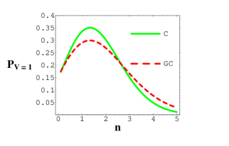
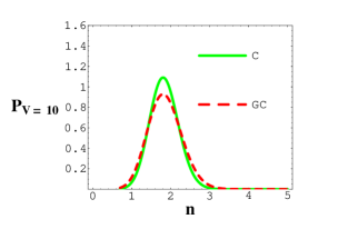
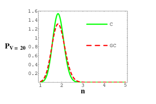
Figure 1: Probability distributions of charged particle density in the canonical and grand canonical ensembles calculated for different volume parameters (V=1, 10 and 20 in arbitrary units).

Knowing the asymptotic properties of the probability distributions on can study the corresponding behavior of the positively and negatively charged particle density moments. The asymptotic behavior of the positively and negatively charged particle density moments in the GC ensemble can be obtained from Eq. (12b) and (28) in the following transparent form

$$_{\langle}{n_{\pm}^{k}}\rangle^{GC}=\langle n_{\pm}\rangle_{\infty}^{k}+\frac{k(k-1)}{2V}\langle n_{\pm}\rangle_{\infty}^{k-1}+\mathcal{O}(V^{-2}),$$ (29)

where $\langle n_{\pm}\rangle_{\infty}$ is as before the average density of $(\pm 1)$– charged particles in the $V\to\infty$ limit which is common for GC and C ensemble. In a particular case, for the second moment $(k=2)$, the Eq.(29) multiplied by $V^{2}$ is a well known result from statistical mechanics: $\langle N^{2}\rangle-\langle N\rangle^{2}=\langle N\rangle$ which tells us that the average square fluctuations in particle number in the GC ensemble are controlled by the average number of particles.

IV Semi-intensive quantities in the thermodynamic limit

As an application of the results for the asymptotic behavior of the probability distributions and charged particle moments we consider the properties of semi–intensive quantities. The simplest example of such a quantity, as discussed in the introduction, is the scaled variance of charged particles

$$\omega_{N_{\pm}}=\frac{\langle N_{\pm}^{2}\rangle-\langle N_{\pm}\rangle^{2}}{\langle N_{\pm}\rangle}\,.$$ (30)

Obviously, one can express $\omega_{N_{\pm}}$ through the corresponding density moments $\omega_{n_{\pm}}$ such as

$$\omega_{N_{\pm}}=V\frac{\langle n_{\pm}^{2}\rangle-\langle n_{\pm}\rangle^{2}}{\langle n_{\pm}\rangle}\equiv V\omega_{n_{\pm}}\,.$$ (31)

The thermodynamic limit of $\omega_{N}$ is controlled by the $(1/V)$– corrections to the first and second moment of the charged particle density. From the results in the previous section it is clear that in the T-limit

$$\langle n^{k}\rangle=\langle n\rangle_{\infty}^{k}+\frac{1}{V}\mathcal{R}_{k;q}+\mathcal{O}(V^{-2})\,,$$ (32)

where the first term is common for the GC and C ensembles, however the $(1/V)$ correction term $\mathcal{R}_{k;q}$ differs in these ensembles. Indeed, from Eq. (20) and (29) one finds

$$\mathcal{R}_{k;q}^{C} = \frac{k(k-1)}{2}\frac{z_{0}^{2}}{x_{q}}\langle n\rangle_{\infty}^{k-2}-k\frac{z_{0}^{2}}{x_{q}^{2}}\langle n\rangle_{\infty}^{k-1}\,,$$ (33)

$$\mathcal{R}_{k;q}^{GC} = \frac{k(k-1)}{2}\langle n\rangle_{\infty}^{k-1}\,,$$ (34)

where $\mathcal{R}^{C}$ and $\mathcal{R}^{GC}$ are the correction terms in C and GC ensemble respectively.

From Eq. (32) it is clear that the ratio

$$\Delta_{k}=\frac{\mathcal{R}_{k;q}}{V\langle n\rangle_{\infty}^{k}}\,,$$ (35)

describes the NLO corrections to the $k$-th order density moment. Following Eqs. (33) and (34) one finds that these corrections for the canonical ensemble

$$\Delta^{C}_{k}=\frac{k(k-1)}{V\langle n\rangle_{\infty}}\,\frac{z_{0}^{2}}{2x_{q}\langle n\rangle_{\infty}}-\frac{k}{V\langle n\rangle_{\infty}}\,\frac{z_{0}^{2}}{x_{q}^{2}}\,,$$ (36)

and for the grand canonical ensemble

$$\Delta^{GC}_{k}=\frac{k(k-1)}{V\langle n\rangle_{\infty}}\,,$$ (37)

are expressed through the total number of particles of a given charge ${V\langle n\rangle_{\infty}}$ as well as through dimensionless variables $z_{0}^{2}/x_{q}\langle n\rangle_{\infty}$ and $z_{0}^{2}/x_{q}^{2}$ which depend only on the $q/z_{0}$ ratio.

From Eq. (21) one finds

$$\frac{q^{2}}{z_{0}^{2}}=\frac{\langle n_{+}\rangle_{\infty}}{\langle n_{-}\rangle_{\infty}}+\frac{\langle n_{-}\rangle_{\infty}}{\langle n_{+}\rangle_{\infty}}-2\,,$$ (38)

thus the NLO corrections $\Delta_{k}$ can be expressed by means of measurable $\langle N_{-}\rangle/\langle N_{+}\rangle$ particles ratios.

In heavy ion collisions at RHIC charged particle ratios like e.g. $\pi^{-}/\pi^{+}$, $K^{-}/K^{+}$ or $\bar{p}/p$ has been measured (see e.g. ratios ) in the range between 0.6 to 1.0. Thus, for RHIC conditions one estimates from Eq. (38) that the relevant domain of $q/z_{0}$ is between 0 and 0.5. In Fig. 2 we calculate from Eqs. (36) and (37) the NLO corrections to the first, the second and the third charge particle density moments for canonical and grand canonical ensemble. These corrections are plotted as a function of the multiplicity of negatively charged particles $\langle N_{-}\rangle$ at fixed value of $\langle N_{-}\rangle/\langle N_{+}\rangle=0.8$ particles ratio.

It is specific for the grand canonical distribution that the first moment $\Delta_{1}$ coincides with its thermodynamic limit. However, as seen in Fig. 2 this is not anymore the case for higher moments where deviations from thermodynamic limit in the GC ensemble are not negligible even for $\langle N_{-}\rangle\simeq 150$. It is also clear from Fig. 2 that for fixed $\langle N_{-}\rangle$ the difference between GC and C ensemble increases with increasing order of particle moments. The convergence of $\Delta_{k}$ to their thermodynamic limit values is slower with increasing $k$, for both ensembles. Finally, it is clear from Fig. 2 that the first moment is converging from below whereas the second and the third from the above to their asymptotic values.

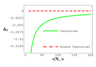
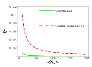
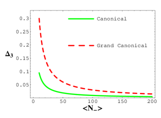
Figure 2: Deviations of the first $\Delta_{1}$, second $\Delta_{2}$ and the third $\Delta_{3}$ charged particle moments from the thermodynamic limit as functions of charge particle multiplicities $\langle N_{-}\rangle$ calculated at fixed $\langle N_{-}\rangle/\langle N_{+}\rangle=0.8$. The results are shown for the canonical and the grand canonical ensembles.

With the above results for the NLO corrections to different particle density moments one can also study the convergence and the thermodynamic limit of the scaled variance (30).

Indeed from Eqs. (31) and (32) one finds:

$$\text{T-}\lim\omega_{N}=\frac{\mathcal{R}_{2;q}-2\mathcal{R}_{1;q}\langle n\rangle_{\infty}}{\langle n\rangle_{\infty}}\,.$$ (39)

Applying in Eq. (39) the C and GC correction factors $\mathcal{R}_{k;q}$ from Eqs. (33) and (34) one gets in the canonical ensemble

$$\text{T-}\lim\mathcal{\omega}_{N}^{C}=\frac{1}{2}\frac{\sqrt{q^{2}+4z_{0}^{2}}\mp q}{\sqrt{q^{2}+4z_{0}^{2}}}\,,$$ (40a)

while in the grand canonical system

$$\text{T-}\lim\mathcal{\omega}_{N}^{GC}=1\,.$$ (40b)

Thus, the scaled variance is finite in the T-limit although it differs in the C and the GC ensembles. This result agrees with the previous finding in begun and explains how to reconcile this with the T-limit equivalence of different statistical ensembles.

The scaled variance is not the only example of semi–intensive variable. There is actually a broad class of variables

$$\mathcal{S}_{k}=\frac{\langle N^{k}\rangle-\langle N\rangle^{k}}{\langle N\rangle^{k-1}}$$ (41a)

which have the same properties as $$\omega_{N}$$: they are finite in T-limit and have different values dependently on how the charge conservation is implemented in the description of the system. Indeed from (32) one gets

$$\text{T-}\lim\mathcal{S}_{k}=\frac{\mathcal{R}_{k;q}-k\mathcal{R}_{1;q}\langle n\rangle_{\infty}^{k-1}}{\langle n\rangle_{\infty}^{k-1}}\,,$$ (41b)

thus, following Eqs. (33–34) the C and GC values for positive(negative) particles in the T-limit are found as

$$\text{T-}\lim\mathcal{S}_{k}^{C}=\frac{k(k-1)}{4}\frac{\sqrt{q^{2}+4z_{0}^{2}}\mp q}{\sqrt{q^{2}+4z_{0}^{2}}}\,,$$ (42a)

while in the grand canonical ensemble

$$\text{T-}\lim\mathcal{S}_{k}^{GC}=\frac{k(k-1)}{2}\,.$$ (42b)

The scaled variance $\omega_{N}$ is just a special case of $S_{k}$ corresponding to $k=2$.

Another example is a broad class of variables closely related to cumulant or factorial cumulant moments $\kappa_{p}$ defined as thi

$$\ln{\mathcal{G}(\operatorname{e}^{\lambda},V)} = \sum\limits_{p}\kappa_{p}\frac{\lambda^{p}}{p!}\qquad\text{for cumulant moments}\,,$$ (43a)

$$\ln{\mathcal{G}(\lambda,V)} = \sum\limits_{p}\kappa_{p}\frac{\lambda^{p}}{p!}\qquad\text{for factorial cumulant moments}\,.$$ (43b)

In the T-limit those moments are linear in $V$, thus the ratios

$$\mathcal{K}_{p;r}=\frac{\kappa_{p}}{\kappa_{r}}\,,$$ (44)

are obviously semi–intensive quantities. For cumulant moments the quantity $\mathcal{K}_{2;1}$ coincides with the scaled variance (1) while for factorial cumulant moments it is equal to $\omega_{N}-1$.

One can also construct more involved semi-inclusive variables having a finite T-limit behavior which are determined by higher order asymptotic terms of the corresponding probability distributions.

V Summary and conclusions

We have considered statistical systems with global charge conservation and discussed the properties of different charged particle probability distributions. We have put particular emphasis on the limiting behavior of the probability densities in their approach towards the thermodynamic limit. In particular we have calculated the asymptotic values and the first subleading finite volume corrections. Our results were obtained in the statistical model of quasi non–interacting gas of charged particles, constrained by the conservation laws. Such a model has been recently shown to be successful in describing particle production in heavy ion collisions and lattice QCD thermodynamics restricted to the confined, hadronic phase.

We have discussed the differences in the asymptotic properties of the probability functions for a system with an exact, that is canonical, (C) and with an average, that is grand canonical, (GC) implementation of charge conservation. We have shown that in the thermodynamic limit the corresponding probability distributions in the GC and C ensembles coincide and are described as generalized functions. This property is a direct consequence of the GC and C ensemble equivalence in the thermodynamic limit. However, the first finite volume corrections to the asymptotic value differ for both ensembles.

Finally, using the results of the probability functions we have derived the asymptotic behavior of the charged particle moments and established the differences in the GC and C formulation. We have also applied these results to find the thermodynamic limit of a class of semi–intensive quantities. It was shown that in systems with exact and average charge conservation such quantities should naturally converge to different values in the thermodynamic limit. This is because the behavior of the semi–intensive quantities in the near vicinity to the thermodynamic limit are determined by the subleading, finite volume, corrections to the probability distributions which are specific to a given statistical ensemble.

Similar conclusions related to the thermodynamic limit in different ensembles can be also drawn for nonrelativistic systems prepar . Such an analysis could be of interest for low energy processes in which the particle number conservation is preserved.

Appendix A Leading and NLO coefficients of $\langle N^{k}\rangle^{C}_{Q}$

The leading and next to leading order contributions to the particle moments $\langle N^{k}\rangle^{C}$ are obtained as the coefficients $c_{k}$ and $c_{k-1}$ at large volume expansion terms in Eq. (15), i.e. from

$$\langle N^{k}\rangle^{C}=c_{k}\,V^{k}+c_{k-1}\,V^{k-1}+\mathcal{O}(V^{k-2})\,.$$ (45)

To get these coefficients using the expansion for the Bessel functions given in (17) we first observe that the second and the third terms in the curly bracket in Eq. (18) can be neglected. This is because the contributions of these terms to the $O(V^{k-1})$ order coefficient exactly cancel each other since the derivative in Eq. (15) is taken at $\lambda=1$. Thus, it is sufficient to consider

$$\mathcal{G}(\lambda,V)\simeq f(\lambda)e^{Vg(\lambda)}$$ (46)

with

$$f(\lambda)=\sqrt{\frac{x_{q}}{x_{q;\lambda}}}\,,\qquad g(\lambda)=x_{q;\lambda}-x_{q}+q\ln\frac{q+x_{q}}{q+x_{q;\lambda}}\,.$$

where $x_{q}$ is as in Eq. (19).

To calculate $c_{k}$ and $c_{k-1}$ we use the identity

$$\left(\lambda\frac{d}{d\lambda}\right)^{k}\mathcal{G}=\lambda^{k}\frac{d^{k}}{d\lambda^{k}}\mathcal{G}+\frac{k(k-1)}{2}\lambda^{k-1}\frac{d^{k-1}}{d\lambda^{k-1}}\mathcal{G}+\cdots$$ (47)

and keep the first two terms with the highest order derivatives. Only the first term in Eq. (47) contributes to $c_{k}$

$$c_{k}=f(\lambda)\left(\frac{dg}{d\lambda}\right)^{k}\operatorname{e}^{Vg(\lambda)}\,.$$ (48)

However, the $c_{k-1}$ coefficient is receiving contributions from both terms in Eq. (47). The highest derivative term in Eq. (47) is calculated from

$$f(\lambda)\frac{d^{k}}{d\lambda^{k}}\operatorname{e}^{Vg(\lambda)}+{k\choose{k-1}}\frac{df}{d\lambda}\frac{d^{k-1}}{d\lambda^{k-1}}\operatorname{e}^{Vg(\lambda)}+\cdots\,\,,$$ (49)

where up to $\mathcal{O}(V^{k-3})$

$$\begin{split}&\frac{d^{k}}{d\lambda^{k}}\operatorname{e}^{Vg(\lambda)}\simeq V^{k}\left(\frac{dg}{d\lambda}\right)^{k}\operatorname{e}^{Vg(\lambda)}+V^{k-1}d_{k}\operatorname{e}^{Vg(\lambda)}\simeq\frac{d}{d\lambda}\left[\frac{d^{k-1}}{d\lambda^{k-1}}\operatorname{e}^{Vg(\lambda)}\right]\simeq\\ &\ \frac{d}{d\lambda}\left[V^{k-1}\left(\frac{dg}{d\lambda}\right)^{k-1}\operatorname{e}^{Vg(\lambda)}+V^{k-2}d_{k-1}\operatorname{e}^{Vg(\lambda)}\right]\,,\end{split}$$ (50)

The coefficients $d_{k}$ obey the following recursion relation

$$d_{k}=d_{k-1}\frac{dg}{d\lambda}+(k-1)\left(\frac{dg}{d\lambda}\right)^{k-2}\frac{d^{2}g}{d\lambda^{2}}\,,$$ (51)

with the solution

$$d_{k}=\frac{k(k-1)}{2}\left(\frac{dg}{d\lambda}\right)^{k-2}\frac{d^{2}g}{d\lambda^{2}}\,.$$ (52)

Applying the above result for $d_{k}$ coefficients in Eq. (50) and using Eq. (47) one gets the final expression for the $c_{k-1}$ coefficient

$$c_{k-1}=\frac{k(k-1)}{2}f(\lambda)\left(\frac{dg}{d\lambda}\right)^{k-1}+k\frac{df}{d\lambda}\left(\frac{dg}{d\lambda}\right)^{k-1}+\frac{k(k-1)}{2}f(\lambda)\left(\frac{dg}{d\lambda}\right)^{k-2}\frac{d^{2}g}{d\lambda^{2}}\,,$$ (53)

where the last term is obtained from the $(k-1)$–order derivative in Eq. (47).

Appendix B Grand Canonical charge density probability distribution in the T-limit

Let us consider the grand canonical probability distribution to find the charge density $q$ in a system of volume $V$ and average charge density $\langle q\rangle$. This probability, following Eq. (10c), reads

$${\mathbf{P}}^{GC}_{\langle q\rangle}(q,V)=V\operatorname{e}^{-Vx_{\langle q\rangle}}I_{Vq}(2Vz_{0})\left[\frac{\langle q\rangle+x_{\langle q\rangle}}{2z_{0}}\right]^{Vq}\,.$$ (54)

with $x_{\langle q\rangle}$ as in Eq. (19) but with $q$ being replaced by $\langle q\rangle$.

Our goal is to find the first subleading contribution to ${\mathbf{P}}^{GC}_{\langle q\rangle}(q,V)$ in the thermodynamic limit.

It is rather straightforward to see from Eq. (54) that the limit $V\to\infty$ for fixed $q$ does not exist as a regular function lt . However, this limit can be found as a generalized function. To show it, we consider the integral

$$\langle G\rangle=\int dqG(q){\mathbf{P}}^{GC}_{\langle q\rangle}(q,V)\,.$$ (55)

where the probability distribution ${\mathbf{P}}^{GC}_{\langle q\rangle}$ is smeared out with a test function $G$.

In our previous study lt it was shown that in the T-limit

$$\langle G\rangle=G(\langle q\rangle)+\mathcal{O}(V^{-1})\,.$$ (56)

Thus, one can write

$$\lim_{V\to\infty}{\mathbf{P}}^{GC}_{\langle q\rangle}(q,V)=\delta\left(q-\langle q\rangle\right)\,.$$ (57)

We apply the asymptotic form of the $I_{\alpha}$ Bessel function (17) in (54) and then calculate the integral (55) using the saddle-point method. To obtain the NLO term of this integral one should take into account contributions coming from the probability (54) in the next to leading order and corresponding contributions from (66) simultaneously.

From (54) and (17, 19) one gets

$$\begin{split}{\mathbf{P}}^{GC}_{\langle q\rangle}(q,V)\simeq&V^{1/2}\frac{e^{-V(x_{\langle q\rangle}-x_{q})}}{\sqrt{2\pi x_{q}}}\left[\frac{\langle q\rangle+x_{\langle q\rangle}}{q+x_{q}}\right]^{Vq}+\\ &V^{-1/2}\frac{6z_{0}^{2}-q^{2}}{12\sqrt{2\pi}x_{q}^{7/2}}\left[\frac{\langle q\rangle+x_{\langle q\rangle}}{q+x_{q}}\right]^{Vq}\operatorname{e}^{-V\left(x_{\langle q\rangle}-x_{q}\right)}\,.\end{split}$$ (58)

The last term in Eq. (58) contributes to the order $\mathcal{O}(V^{-1})$ in ${\mathbf{P}}^{GC}_{\langle q\rangle}(q,V)$ as

$$\frac{1}{V}\frac{6z_{0}^{2}-q^{2}}{12\sqrt{2\pi}x_{q}^{3}}\delta(q-\langle q\rangle)\,.$$ (59)

A further contribution of order $\mathcal{O}(V^{-1})$ comes from the coefficient $c_{1}$ calculated from Eq. (66) as

$$c_{1}=\frac{\sqrt{\pi}}{4}\left(\frac{d}{dy}\right)^{2}\left.\left[\frac{G(y)}{\sqrt{2\pi}(y^{2}+4z_{0}^{2})^{1/4}}\left(\frac{S(y_{0})-S(y)}{(y-y_{0})^{2}}\right)^{-3/2}\right]\right|_{y=y_{0}}\,.$$ (60)

with

$$S(q)=x_{q}-x_{\langle q\rangle}+q\ln\frac{\langle q\rangle+x_{\langle q\rangle}}{q+x_{q}}\,.$$ (61)

This gives

$$c_{1}=\frac{1}{12}\frac{\langle q\rangle^{2}-6z_{0}^{2}}{x_{\langle q\rangle}^{3}}G(\langle q\rangle)+\frac{x_{\langle q\rangle}}{2}G^{{}^{\prime\prime}}(\langle q\rangle)\,.$$ (62)

Consequently, the leading and the subleading contributions to ${\mathbf{P}}^{GC}_{\langle q\rangle}(q,V)$ are obtained as

$${\mathbf{P}}^{GC}_{\langle q\rangle}(q,V)=\delta\left(q-\langle q\rangle\right)+\frac{x_{\langle q\rangle}}{2V}\,\delta^{{}^{\prime\prime}}(q-\langle q\rangle)+\mathcal{O}(V^{-2})\,,$$ (63)

where the double prime in the delta function is the second derivative with respect to the charge density $q$.

Appendix C Watson-Laplace theorem

Let us consider the Laplace integral

$$F(\lambda)=\int\limits_{I}dx\operatorname{e}^{\lambda S(x)}f(x)\,.$$ (64)

An asymptotic expansion of $F(\lambda)$ in the limit $\lambda\to\infty$ is given by the classical Watson-Laplace theorem:

Let $I=[a,b]$ be a finite interval such that

1. $\max\limits_{x\in I}S(x)$ is reached only in the single point $x_{0}=a,\ a<x_{0}<b$.

2. $f(x),S(x)\in C(I)$.

3. $f(x),S(x)\in C^{\infty}$ in the vicinity of $x_{0}$, and $S^{{}^{\prime\prime}}(x_{0})\neq 0$ .

Then, for $\lambda\in S_{\epsilon}$ and $\lambda\to\infty$,  the following expansion holds

$$F[\lambda]\simeq\operatorname{e}^{\lambda S(x_{0})}\sum\limits_{k=0}^{\infty}c_{k}\lambda^{-k-1/2}\,,$$ (65)

where the coefficients

$$c_{k}=\frac{\Gamma(k+1/2)}{(2k)!}\left(\frac{d}{dx}\right)^{2k}\left.\left[f(x)\left(\frac{S(x_{0})-S(x)}{(x-x_{0})^{2}}\right)^{-k-1/2}\right]\right|_{x=x_{0}}\,.$$ (66)

$S_{\epsilon}$ is here a segment $|\arg z|\leqslant\frac{\pi}{2}-\epsilon<\frac{\pi}{2}$ in the complex $z$-plane.

References

• (1) For a recent review see e.g., P. Braun-Munzinger, K. Redlich and J. Stachel, Quark Gluon Plasma 3 (Edts. R. C. Hwa and X. N. Wang), nucl - th/0304013; A. Andronic and P. Braun-Munzinger, hep-ph/0402291.
• (2) V. Koch, Nucl. Phys. A 715, 108 (2002); D. Rischke, Nucl. Phys. A 698, 153 (2002); R. Hagedorn, Nuovo Cimento 35, 395 (1965); R. Hagedorn, Thermodynamics of strong interactions, CERN Report 71-12 (1971); R. Venugopalan and M. Prakash, Nucl. Phys. A 546, 718 (1992).
• (3) C. R. Allton, M. Döring, S. Ejiri, S. J. Hands, O. Kaczmarek, F. Karsch, E. Laermann and K. Redlich, hep-lat/0501030; S. Ejiri, C. R. Allton, M. Döring, S. J. Hands, O. Kaczmarek, F. Karsch, E. Laermann and K. Redlich, hep-lat/0409033; hep-lat/0408046.
• (4) F. Karsch, K. Redlich and A. Tawfik, Eur. Phys. J. C 29, 549 (2003); Phys. Lett. B 571, 67 (2003); K. Redlich, hep-ph/0406250.
• (5) M. D’Elia and Maria–Paola Lombardo, hep-lat/0409010.
• (6) K. Redlich and L. Turko, Z. Phys. C 5, 201 (1980); L. Turko, Phys. Lett. B 104, 153 (1981).
• (7) R. Hagedorn and K. Redlich, Z. Phys. C 27, 541 (1985).
• (8) J. Rafelski and M. Danos, Phys. Lett. B 97, 279 (1980); B. Muller and J. Rafelski, Phys. Lett. B 116, 274 (1982).
• (9) M. I. Gorenstein, S. I. Lipskikh, V. K. Petrov and G. M. Zinovev, Phys. Lett. B 123, 437 (1983); H. T. Elze, W. Greiner and J. Rafelski, Phys. Lett. B 124, 515 (1983); J. Cleymans, K. Redlich and E. Suhonen, Z. Phys. C 51, 137 (1991); J. Cleymans, A. Keränen, M. Marais and E. Suhonen, Phys. Rev. C 56, 2747 (1997); M. I. Gorenstein, M. Gazdzicki and W. Greiner, Phys. Lett. B 483, 60 (2000).
• (10) J. Cleymans, H. Oeschler and K. Redlich, Phys. Rev. C 59, 1663 (1999);
• (11) V. V. Begun, M. Gazdzicki, M. I. Gorenstein and O. S. Zozulya, Phys. Rev. C 70, 034901 (2004); V. V. Begun, M. I. Gorenstein, A. P. Kostyuk and O. S. Zozulya, Phys. Rev. C 71, 054904 (2005); A. Keranen, F. Becattini, V. V. Begun, M. I. Gorenstein and O. S. Zozulya, J. Phys. G 31, S1095 (2005).
• (12) J. Cleymans, K. Redlich and L. Turko, Phys. Rev. C 71, 047902 (2005).
• (13) C.R. Allton, S. Ejiri, S.J. Hands, O. Kaczmarek, F. Karsch, E. Laermann, C. Schmidt and L. Scorzato, Phys. Rev. D 66, 074507 (2002).
• (14) M. Gazdzicki et al. [NA49 Collaboration], J. Phys. G 30, S701 (2004); M. Rybczynski et al. [NA49 Collaboration], J. Phys. Conf. Ser. 5, 74 (2005), nucl-ex/0409009.
• (15) C. M. Ko, V. Koch, Z. Lin, K. Redlich, M. Stephanov and X. N. Wang, Phys. Rev. Lett. 86, 5438 (2001); Z. Lin and C. M. Ko, Phys. Rev. C 64, 041901 (2001); S. Jeon, V. Koch, K. Redlich and X. N. Wang, Nucl. Phys. A 697, 546 (2002); K. Redlich, V. Koch and A. Tounsi, Nucl. Phys. A 702, 326 (2002); K. Redlich, J. Cleymans, H. Oeschler, and A. Tounsi, Acta Phys. Polon. B 33, 1609 (2002).
• (16) M. Abramowitz and I.A. Stegun, Handbook of Mathematical Functions, (NBS 1964)
• (17) T. Thiele, The Theory of Observations. Charles & Edwin Layton, London, 1903. Ann. Math. Stat., 2, 165 (1931); A. H. Mueller, Phys. Rev. D 4, 150 (1971)
• (18) I. G. Bearden et al.[BRAHMS Collaboration], Phys. Rev. Lett. 90, 102301 (2003); B. B. Back et al.[PHOBOS Collaboration], Phys. Rev. C 67, 021901 (2003); S. S. Adler et al.[PHENIXCollaboration], Phys. Rev. C 69, 034909 (2004); J. Adams et al.[STAR Collaboration], Phys. Rev. C 70, 044901 (2004); J. Adams et al.[STAR Collaboration], Nucl. Phys. A 757, 102 (2005) and references therein
• (19) L. Turko, in preparation