Scattering of a Klein-Gordon particle by a Woods-Saxon potential

Abstract

We solve the Klein-Gordon equation in the presence of a spatially one-dimensional Woods-Saxon potential. The scattering solutions are obtained in terms of hypergeometric functions and the condition for the existence of transmission resonances is derived. It is shown how the zero-reflection condition depends on the shape of the potential.

Recently, the Woods-Saxon potential and their supersymmetric extensions have been extensively discussed in the literature Guo ; Petrillo ; Chen ; Guo2 ; Alhaidari . Among the advantages of working with the Woods-Saxon potential we have to mention that, in the one-dimensional case, the Klein-Gordon as well as the Dirac equations are solvable in terms of special functions and therefore the study of bound states and scattering processes becomes more tractable. It should be mentioned that the Woods saxon potential is, for some values of the shape parameters, a smoothed out form of the potential barrier.

The study of low momentum scattering in the Schrödinger equation in one-dimensional even potentials shows that, as momentum goes to zero, the reflection coefficient goes to unity unless the potential $V(x)$ supports a zero energy resonance Newton . In this case the transmission coefficient goes to unity, becoming a transmission resonance Bohm . Recently, this result has been generalized to the Dirac equation Dombey , showing that transmission resonances at $k=0$ in the Dirac equation take place for a potential barrier $V=V(x)$ when the corresponding potential well $V=-V(x)$ supports a supercritical state. The situation for short range potentials in the Klein-Gordon equation is completely different, here there are particle-antiparticle creation processes but no supercritical states Schiff ; Snyder ; greiner ; Greiner2 ; Rafelski ; Popov . The absence of supercritical states in the Klein-Gordon equation in the presence of short-range potential interactions does not prevent the existence of transmission resonances for given values of the potential.

The presence of transmission resonances in relativistic scalar wave equations in external potentials has been extensively discussed in the literature greiner ; Fulling . As a result of this phenomenon we have that, for given values of the energy and of the shape of the effective barrier, the probability of the transmission coefficient reaches a maximum such as those obtained in the study of quasinormal modes and superradiance in black hole physics.

Despite its relative simplicity, scattering processes of relativistic scalar particles by one-dimensional potentials exhibit the same physical properties that $s$ waves in the presence of radial potentials, therefore the results reported in this article can be straightforwardly extended to the radial Woods-Saxon potential.

It is the purpose of the present article to compute the scattering solutions of the one-dimensional Klein-Gordon equation in the presence of a Woods-Saxon potential and show that one-dimensional scalar wave solutions exhibit transmission resonances with a functional dependence on the shape and strength of the potential similar to the obtained for the Dirac equation kennedy .

The one-dimensional Klein-Gordon equation, minimally coupled to a vector potential $A^{\mu}$ can be written as

$$\eta^{\alpha\beta}(\partial_{\alpha}+ieA_{\alpha})(\partial_{\beta}+ieA_{\beta})\phi+\phi=0$$ (1)

where the metric $\eta^{\alpha\beta}=diag(1,-1)$ and here and thereafter we choose to work in natural units $\hbar=c=m=1$ greiner

$$\frac{d^{2}\phi(x)}{dx^{2}}+\left[\left(E-V(x)\right)^{2}-1\right]\phi(x)=0.$$ (2)

The Woods-Saxon potential is defined as kennedy

$$V(x)=V_{0}\left[\frac{\Theta(-x)}{1+e^{-a(x+L)}}+\frac{\Theta(x)}{1+e^{a(x-L)}}\right],$$ (3)

where $V_{0}$ is real and positive; $a>0$ and $L>0$ are also real and positive. $\Theta(x)$ is the Heaviside step function. The form of the Woods-Saxon potential is shown in the Fig. 1.

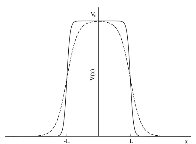
Figure 1: Woods-Saxon potential for $L=2$ with $a=10$ (solid line) and $a=3$ (dotted line).

From Fig. 1 one readily notices that, for a given value of the width parameter $L$, as the shape parameter $a$ increases, the Woods-Saxon potential reduces to a square barrier with smooth walls.

In order to consider the scattering solutions for $x<0$ with $E^{2}>1$, we proceed to solve the differential equation

$$\frac{d^{2}\phi_{L}(x)}{dx^{2}}+\left[\left(E-\frac{V_{0}}{1+e^{-a(x+L)}}\right)^{2}-1\right]\phi_{L}(x)=0.$$ (4)

On making the substitution $y=-e^{-a(x+L)}$ , Eq. (4) becomes

$$a^{2}y\frac{d}{dy}\left[y\frac{d\phi_{L}(y)}{dy}\right]+\left[\left(E-\frac{V_{0}}{1-y}\right)^{2}-1\right]\phi_{L}(y)=0.$$ (5)

Putting $\phi_{L}(y)=y^{\mu}(1-y)^{-\lambda_{1}}h(y)$, Eq. (5) reduces to the hypergeometric equation

$$y(1-y)h^{\prime\prime}+[(1+2\mu)-(2\mu-2\lambda_{1}+1)y]h^{\prime}-(\mu-\lambda_{1}+\nu)(\mu-\lambda_{1}-\nu)h=0,$$ (6)

where the primes denote derivatives with respect to $y$ and the parameters $\nu,$ $k,$ $\mu,$, $\lambda$ and $\lambda_{1}$ are:

$$\nu=\frac{ik}{a},\hskip 28.45274ptk=\sqrt{E^{2}-1,}\hskip 28.45274pt\mu=\frac{\sqrt{1-(E-V_{0})^{2}}}{a},$$ (7)

$$\lambda=\frac{\sqrt{a^{2}-4V_{0}^{2}}}{2a},\hskip 28.45274pt\lambda_{1}=-\frac{1}{2}+\lambda.$$ (8)

The general solution of Eq. (6) can be expressed in terms of Gauss hypergeometric functions ${{}_{2}F_{1}}\left(\mu,\nu,\lambda;y\right)$ as abra

$$h(y) = D_{1}\hskip 1.42271pt{{}_{2}F_{1}}\left(\mu-\nu-\lambda_{1},\mu+\nu-\lambda_{1},1+2\mu;y\right)$$ (9)

$$+ D_{2}\hskip 1.42271pty^{-2\mu}{{}_{2}F_{1}}\left(-\mu-\nu-\lambda_{1},-\mu+\nu-\lambda_{1},1-2\mu;y\right),$$

so

$$\phi_{L}(y) = D_{1}y^{\mu}(1-y)^{-\lambda_{1}}\hskip 1.42271pt_{2}F_{1}\left(\mu-\nu-\lambda_{1},\mu+\nu-\lambda_{1},1+2\mu;y\right)$$ (10)

$$+ D_{2}y^{-\mu}(1-y)^{-\lambda_{1}}\hskip 1.42271pt_{2}F_{1}\left(-\mu-\nu-\lambda_{1},-\mu+\nu-\lambda_{1},1-2\mu;y\right).$$

As $x\rightarrow-\infty$, we have that $y\rightarrow-\infty$, and the asymptotic behavior of the solutions (10) can be determined using the asymptotic behavior of the Gauss hypergeometric functions abra

$$_{2}F_{1}(a,b,c;y)=\frac{\Gamma(c)\Gamma(b-a)}{\Gamma(b)\Gamma(c-a)}(-y)^{-a}+\frac{\Gamma(c)\Gamma(a-b)}{\Gamma(a)\Gamma(c-b)}(-y)^{-b}.$$ (11)

Using Eq. (11) and noting that in the limit $x\rightarrow-\infty$, $(-y)^{\mp\nu}\rightarrow e^{\pm ik(x+L)}$  we have that the asymptotic behavior of $\phi_{L}(x)$ can be written as

$$\phi_{L}(x)\rightarrow Ae^{ik(x+L)}+Be^{-ik(x+L)},$$ (12)

where the coefficients $A$ and $B$ in Eq. (12) can be expressed in terms of $D_{1}$ and $D_{2}$ as:

$$A=D_{1}\frac{\Gamma(1-2\mu)\Gamma(-2\nu)(-1)^{-\mu}}{\Gamma(-\mu-\nu-\lambda_{1})\Gamma(1-\mu-\nu+\lambda_{1})}+D_{2}\frac{\Gamma(1+2\mu)\Gamma(-2\nu)(-1)^{\mu}}{\Gamma(\mu-\nu-\lambda_{1})\Gamma(1+\mu-\nu+\lambda_{1})}.$$ (13)

$$B=D_{1}\frac{\Gamma(1-2\mu)\Gamma(2\nu)(-1)^{-\mu}}{\Gamma(-\mu+\nu-\lambda_{1})\Gamma(1-\mu+\nu+\lambda_{1})}+D_{2}\frac{\Gamma(1+2\mu)\Gamma(2\nu)(-1)^{\mu}}{\Gamma(\mu+\nu-\lambda_{1})\Gamma(1+\mu+\nu+\lambda_{1})}.$$ (14)

Now we consider the solution for $x>0$.  In this case, the differential equation to solve is

$$\frac{d^{2}\phi_{R}(x)}{dx^{2}}+\left[\left(E-\frac{V_{0}}{1+e^{a(x-L)}}\right)^{2}-1\right]\phi_{R}(x)=0.$$ (15)

The analysis of the solution can be simplified making the substitution $z^{-1}=1+e^{a(x-L)}$. Eq. (15) can be written as

$$a^{2}z(1-z)\frac{d}{dz}\left[z(1-z)\frac{d\phi_{R}(z)}{dz}\right]+\left[\left(E-V_{0}z\right)^{2}-1\right]\phi_{R}(z)=0.$$ (16)

Putting $\phi_{R}(z)=z^{-\nu}(1-z)^{-\mu}g(z)$, Eq. (16) reduces to the hypergeometric equation

$$z(1-z)g^{\prime\prime}+[(1-2\nu)-2(1-\nu-\mu)z]g^{\prime}-\left({\scriptstyle\frac{1}{2}}-\nu-\mu-\lambda\right)\left({\scriptstyle\frac{1}{2}}-\nu-\mu+\lambda\right)g=0,$$ (17)

where the primes denote derivatives with respect to $z.$ The general solution of Eq. (17) is abra

$$g(z) = d_{1}\hskip 1.42271pt{}_{2}F_{1}\left({\scriptstyle\frac{1}{2}}-\nu-\mu-\lambda,{\scriptstyle\frac{1}{2}}-\nu-\mu+\lambda,1-2\nu;z\right)$$ (18)

$$+ d_{2}z^{2\nu}\hskip 1.42271pt_{2}F_{1}\left({\scriptstyle\frac{1}{2}}+\nu-\mu-\lambda,{\scriptstyle\frac{1}{2}}+\nu-\mu+\lambda,1+2\nu;z\right),$$

so, the solution of Eq. (15) can be written as:

$$\phi_{R}(z) = d_{1}z^{-\nu}(1-z)^{-\mu}\hskip 1.42271pt_{2}F_{1}\left({\scriptstyle\frac{1}{2}}-\nu-\mu-\lambda,{\scriptstyle\frac{1}{2}}-\nu-\mu+\lambda,1-2\nu;z\right)$$ (19)

$$+ d_{2}z^{\nu}(1-z)^{-\mu}\hskip 1.42271pt_{2}F_{1}\left({\scriptstyle\frac{1}{2}}+\nu-\mu-\lambda,{\scriptstyle\frac{1}{2}}+\nu-\mu+\lambda,1+2\nu;z\right).$$

Keeping only the solution for the transmitted wave, $d_{2}=0$ in Eq. (19), we have that in the limit $x\rightarrow\infty$, $z$ goes to zero and $z^{-1}\rightarrow e^{a(x-L)}$. $\phi_{R}(x)$ can be written as

$$\phi_{R}(x)\rightarrow d_{1}e^{ik(x-L)}$$ (20)

The electrical current density for the one-dimensional Klein-Gordon equation (1) is given by the expression:

$$\vec{j}=\frac{i}{2}\left(\phi^{\ast}\vec{\nabla}\phi-\phi\vec{\nabla}\phi^{\ast}\right)$$ (21)

The current as $x\rightarrow-\infty$ can be decomposed as $j_{L}=j_{in}-j_{refl}$ where $j_{in}$ is the incident current and $j_{refl}$ is the reflected one. Analogously we have that, on the right side, as $x\rightarrow\infty$ the current is $j_{R}=j_{trans}$, where $j_{trans}$ is the transmitted current.

Using the reflected $j_{refl}$ and transmitted $j_{trans}$ currents, we have that the reflection coefficient $R$, and the transmission coefficient $T$ can be expressed in terms of the coefficients $A$, $B$ and $d_{1}$ as:

$$R=\frac{j_{refl}}{j_{inc}}=\frac{|B|^{2}}{|A|^{2}},$$ (22)

$$T=\frac{j_{trans}}{j_{inc}}=\frac{|d_{1}|^{2}}{|A|^{2}}$$ (23)

Obviously, $R$ and $T$ are not independent, they are related via the unitarity condition

$$R+T=1$$ (24)

In order to obtain $R$ and $T$ we proceed to equate at $x=0$ the right $\phi_{R}$ and left $\phi_{L}$ wave functions and their first derivatives. From the matching condition we derive a system of equations governing the dependence of coefficients $A$ and $B$ on $d_{1}$ that can be solved numerically. Fig. 2, 3, show the transmission coefficients $T$, for $a=2$, $L=2$, Fig. 4 and 5 show the transmission coefficients $T$, for $a=10$ and $L=2$.

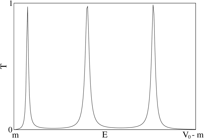
Figure 2: The transmission coefficient for the relativistic Woods-Saxon potential barrier. The plot illustrates $T$ for varying energy, $E$ with $a=2$, $L=2$, $m=1$ and $V_{0}=4$.

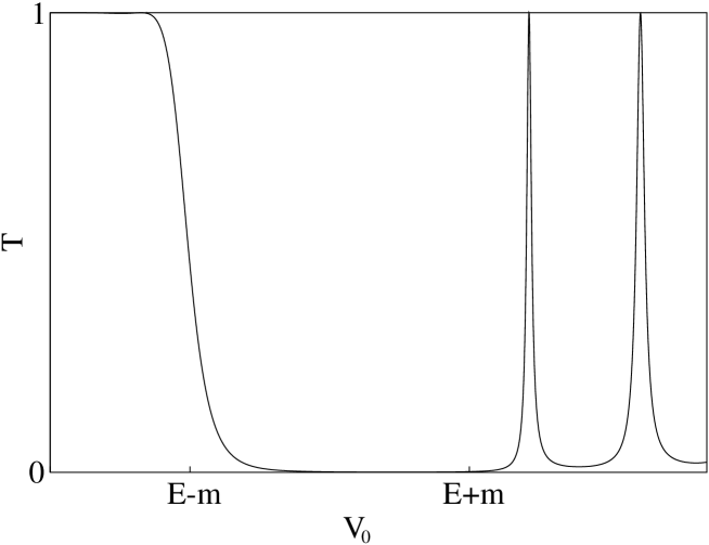
Figure 3: The transmission coefficient for the relativistic Woods-Saxon potential barrier. The plot illustrates $T$ for varying barrier height, $V_{0}$ with $a=2$, $L=2$, $m=1$ and $E=2m$.

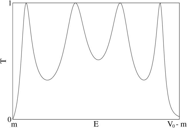
Figure 4: The transmission coefficient for the relativistic Woods-Saxon potential barrier. The plot illustrates $T$ for varying energy, $E$ with $a=10$, $L=2$, $m=1$ and $V_{0}=4$.

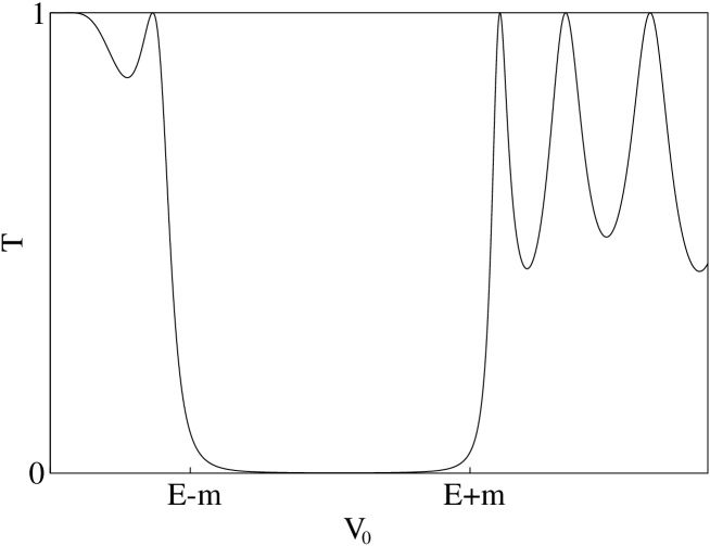
Figure 5: The transmission coefficient for the relativistic Woods-Saxon potential barrier. The plot illustrates $T$ for varying barrier height, $V_{0}$ with $a=10$, $L=2$, $m=1$ and $E=2m$.

From Fig. 2 and Fig. 4 we can see that, analogous to the Dirac particle, the Klein-Gordon particle exhibits transmission resonances in the presence of the one-dimensional Woods-Saxon potential. Fig. 2 and Fig. 4 also show that the width of the transmission resonances depend on the shape parameter $a$ becoming wider as the Woods-Saxon potential approaches to a square barrier.

Fig. 3 and Fig. 5 show that, as in the Dirac case, the transmission coefficient vanishes for values of the potential strength $E-m<V_{0}<E+m$ and transmission resonances appear for $V_{0}>E+m$. Fig. 3 and Fig. 5 also show that the width of the transition resonances decreases as the parameter $a$ decreases. We also conclude that, despite the fact that the behavior of supercritical states for the Klein-Gordon equation in the presence of short-range potentials is qualitatively different from the one observed for Dirac particles Popov , transmission resonances for the one-dimensional Klein-Gordon equation possess the same rich structure that we observe for the Dirac equation.

References

(1) J. Y. Guo, X. Z. Fang, F. X. Xu, Phys. Rev. A. 66,
062105 (2003).
(2) V. Petrillo and D. Janner, Phys. Rev. A. 67,
012110 (2003).
(3) G. Chen, Phys. Scripta 69, 257 (2004).
(4) J. Y. Guo, J. Meng, and F. X. Xu, Chinese Phys. Lett.
20, 602 (2003).
(5) A. D. Alhaidari, Phys. Rev. Lett. 87, 210405
(2001); Phys. Rev. Lett. 88, 189901 (2002).
(6) R. Newton, Scattering Theory of Waves and Particles
(Springer-Verlag, Berlin 1982).