A new method to solve the Non Perturbative Renormalization Group equations

Abstract

We propose a method to solve the Non Perturbative Renormalization Group equations for the $n$-point functions. In leading order, it consists in solving the equations obtained by closing the infinite hierarchy of equations for the $n$-point functions. This is achieved: i) by exploiting the decoupling of modes and the analyticity of the $n$-point functions at small momenta: this allows us to neglect some momentum dependence of the vertices entering the flow equations; ii) by relating vertices at zero momenta to derivatives of lower order vertices with respect to a constant background field. Although the approximation is not controlled by a small parameter, its accuracy can be systematically improved. When it is applied to the $O(N)$ model, its leading order is exact in the large $N$ limit; in this case, one recovers known results in a simple and direct way, i.e., without introducing an auxiliary field.

ECT*– 05-02

1 Introduction

In the last ten years a considerable amount of effort has been devoted to the study of the Non Perturbative Renormalization Group (NPRG), and to the development of new approximation schemes to solve the corresponding infinite hierarchy of equations for the $n$-point functions [1, 2, 3, 4]. In this context, the so-called “derivative expansion” has been widely used. It defines a systematic approach that has led to many successful applications in a variety of domains [5, 6, 7]. However, the derivative expansion is a good approximation to $n$-point functions only when the external momenta are smaller than the lowest mass in the problem. In particular, for massless theories, the derivative expansion provides information only on the $n$-point functions (and their derivatives) at zero momenta. This is not enough for applications which require the knowledge of the full momentum dependence of the $n$-point functions. In these cases, a new approximation scheme is necessary.

To our knowledge, all efforts in this direction [9] have been based on various forms of the early proposal by Weinberg [8]: one truncates the infinite tower of flow equations for the $n$-point functions considering only vertices up to a given number of legs, possibly using various ansatzs for some of them. This leads to approximations similar to those used when solving Schwinger-Dyson equations [10]. However, despite the fact that very encouraging results have been obtained problems remain with truncations around zero external fields [11].

It is then interesting to look for alternative schemes to solve NPRG at finite external momenta and it is the purpose of this Letter to present a method to calculate correlation functions at arbitrary momenta within the NPRG. As it is the case for the derivative expansion, the proposed strategy takes into account, at each order, an infinite number of vertices. The accuracy is expected to be comparable to that achieved with the derivative expansion when it is used to calculate the effective potential. The method exploits two properties of the NPRG: the decoupling of short wave-length modes, and the analyticity of the $n$-point functions at small momentum (guaranteed by the infrared regulator), in order to neglect some of the momentum dependence in the vertices which enter the flow equations. Then, it becomes possible to close the infinite hierarchy of equations by calculating vertices at zero momenta as derivatives of lower order vertices with respect to a constant background field. Although the approximation is not controlled by any small parameter, its accuracy can be systematically improved, in a way similar to what can be done in the derivative expansion.

The leading order of the proposed approximation scheme shares some of the nice properties of the leading order of the derivative expansion, the so-called local potential approximation (LPA): it is exact at one loop order, and it also reproduces the exact large $N$ limit of the $O(N)$ model. Of course, the LPA provides only information on momentum independent quantities, such as the effective potential, whereas the present method does not have this limitation. In fact, as an illustration, we use it to solve the NPRG equations for the full momentum dependent $n$-point functions of the $O(N)$ model in the large $N$ limit. This can be done directly, i.e., without having to introduce an auxiliary field. To our knowledge, this is the first time that, within the NPRG, such a calculation is done for this model.

The method presented here is an improvement of the one that we have applied in a previous paper to the calculation of the transition temperature of a weakly repulsive Bose gas [12]. Compared to the method proposed in [12], the present one is conceptually simpler as it involves a single approximation. Its numerical implementation will be discussed in a separate publication [13].

2 The NPRG and the derivative expansion

Let us start by recalling some basic features of the NPRG. Although most of the arguments in this paper have a wider range of applicability, we shall consider a scalar field theory defined by an Euclidean action $S$ in $d$ dimensions, of the generic form:

$$S=\int{\rm d}^{d}x\,\left\{{1\over 2}\left(\partial_{\mu}\varphi(x)\right)^{2}+V(\varphi)\right\}\,,$$ (1)

where $V(\varphi)$ is a polynomial in $\varphi$. It is understood that the parameters of the action (hidden in $V(\varphi)$) and the field normalization are fixed at a microscopic momentum scale $\Lambda$ (which may be infinite). The NPRG equations relate the classical action to the full effective action. This relation is obtained by controlling the magnitude of long wavelength field fluctuations with the help of an infrared cut-off, which is implemented [1, 2, 3, 4] by adding to the classical action (1) a regulator of the form

$$\Delta S_{\kappa}[\varphi]=\frac{1}{2}\int\frac{{\rm d}^{d}p}{(2\pi)^{d}}R_{\kappa}(p)\varphi(p)\varphi(-p),$$ (2)

where $R_{\kappa}$ denotes a family of “cut-off functions” depending on a parameter $\kappa$. The role of $\Delta S_{\kappa}$ is to suppress the fluctuations with momenta $p\mathrel{\hbox to0.0pt{\raise 2.20013pt\hbox{$<$}\hss}{\lower 2.20013pt\hbox{$\sim$}}}\kappa$, while leaving unaffected the modes with $p\mathrel{\hbox to0.0pt{\raise 2.20013pt\hbox{$>$}\hss}{\lower 2.20013pt\hbox{$\sim$}}}\kappa$. Thus, typically $R_{\kappa}(p)\to\kappa^{2}$ when $p\ll\kappa$, and $R_{\kappa}(p)\to 0$ when $p\mathrel{\hbox to0.0pt{\raise 2.20013pt\hbox{$>$}\hss}{\lower 2.20013pt\hbox{$\sim$}}}\kappa$. There is a large freedom in the choice of $R_{\kappa}(p)$, abundantly discussed in the literature [14, 15, 16, 17].

We denote the effective action in the presence of the regulator by $\Gamma_{\kappa}[\phi]$, where $\phi$ is the average field, $\phi(x)=\left\langle\varphi(x)\right\rangle$. When $\kappa\to\Lambda$ quantum fluctuations are suppressed and $\Gamma_{\Lambda}[\phi]$ coincides with the classical action. As $\kappa$ decreases, more and more quantum fluctuations are taken into account and, as $\kappa\to 0$, $\Gamma_{\kappa=0}[\phi]$ becomes the usual effective action $\Gamma[\phi]$. In other words, as $\kappa$ decreases from $\Lambda$ to $0$, $\Gamma_{\kappa}$ interpolates between the classical action and the full effective action (see e.g. [5]). The variation with $\kappa$ of $\Gamma_{\kappa}[\phi]$ is governed by the following flow equation [1, 2, 3, 4]:

$$\partial_{\kappa}\Gamma_{\kappa}[\phi]=\frac{1}{2}\int\frac{d^{d}q}{(2\pi)^{d}}\partial_{\kappa}R_{\kappa}(q^{2})\left[\Gamma_{\kappa}^{(2)}+R_{\kappa}\right]^{-1}_{q,-q},$$ (3)

where $\Gamma_{\kappa}^{(2)}$ is the second derivative of $\Gamma_{\kappa}$ w.r.t. $\phi$ (see Eq. (5) below). Eq. 3 is the master equation of the NPRG. Its right hand side has the structure of a one loop integral, with one insertion of $\partial_{\kappa}R_{\kappa}(q^{2})$.

As well known [18], the effective action $\Gamma[\phi]$ is the generating functional of the one-particle irreducible $n$-point functions. Similarly, for a given value of $\kappa$, we define the $n$-point functions $\Gamma_{\kappa}^{(n)}$:

$$\Gamma_{\kappa}^{(n)}(p_{1},\dots,p_{n})=\int d^{d}x_{1}\dots\int d^{d}x_{n-1}e^{i\sum_{j=1}^{n}p_{j}x_{j}}\frac{\delta^{n}\Gamma_{\kappa}}{\delta\phi(x_{1})\dots\delta\phi(x_{n})}.$$ (4)

By deriving eq. (3) with respect to $\phi$, and then letting the field be constant, one gets the flow equations for all $n$-point functions in a constant background field $\phi$. These equations can be represented diagramaticaly by one loop diagrams with dressed vertices and propagators (see e.g. [19]). For instance, the flow of the 2-point function in a constant external field reads:

$$\partial_{\kappa}\Gamma_{\kappa}^{(2)}(p,-p;\phi) = \int\frac{d^{d}q}{(2\pi)^{d}}\partial_{\kappa}R_{k}(q)\left\{G_{\kappa}(q^{2};\phi)\Gamma_{\kappa}^{(3)}(p,q,-p-q;\phi)\right.$$ (5)

$$\times G_{\kappa}((q+p)^{2};\phi)\Gamma_{\kappa}^{(3)}(-p,p+q,-q;\phi)G_{\kappa}(q^{2};\phi)$$

$$\left.-\frac{1}{2}G_{\kappa}(q^{2};\phi)\Gamma_{\kappa}^{(4)}(p,-p,q,-q;\phi)G_{\kappa}(q^{2};\phi)\right\},$$

where

$$G^{-1}_{\kappa}(q^{2};\phi)=\Gamma^{(2)}_{\kappa}(q,-q;\phi)+R_{\kappa}(q^{2}).$$ (6)

The corresponding diagrams contributing to the flow are shown in Fig. 1.

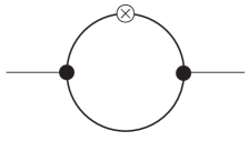
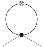
Figure 1: The two diagrams contributing to the flow of the 2-point vertex. The lines represent dressed propagators, $G_{\kappa}$. The cross represents an insertion of $\partial_{\kappa}R_{k}$. The vertices denoted by black dots are $\Gamma^{(3)}_{\kappa}$ and $\Gamma^{(4)}_{\kappa}$.

Flow equations for the $n$-point functions do not close: for example, in order to solve eq. (5) one needs the 3- and the 4-point functions, $\Gamma_{\kappa}^{(3)}$ and $\Gamma_{\kappa}^{(4)}$ respectively. At this point we observe that because of the shape of the regulator, only internal momenta $q$ smaller than $\kappa$ contribute to the flow, i.e., to the integral in the r.h.s. of eq. (5). One refers to this property as to the decoupling of high momentum modes. Besides, the regulator insures also that all vertices are smooth functions of momenta. Suppose then that one wants to calculate $n$-point functions at small external momenta, say, $p_{i}^{2}\mathrel{\hbox to0.0pt{\raise 2.20013pt\hbox{$<$}\hss}{\lower 2.20013pt\hbox{$\sim$}}}\kappa^{2}$. Then all momenta are small. This, together with the fact that the $n$-point functions are smooth functions of the momenta, make it possible to expand the $n$-point functions $\Gamma_{\kappa}^{(n)}$ in the r.h.s. of the flow equations in terms of $q^{2}/\kappa^{2}$ and $p^{2}/\kappa^{2}$, or equivalently in terms of the derivatives of the field.

Such considerations are at the basis of the derivative expansion, which is usually formulated in terms of an ansatz for the effective action, rather than in terms of an approximation for the $n$-point functions. Its zero order, the LPA, assumes that the effective action has the form:

$$\Gamma_{k}^{LPA}[\phi]=\int d^{d}x\left\{\frac{1}{2}\partial_{\mu}\phi\partial_{\mu}\phi+V_{k}(\phi)\right\}.$$ (7)

The derivative term here is simply the one appearing in the classical action, and $V_{k}(\phi)$ is the effective potential. The flow equation for $V_{\kappa}$ is a closed equation that is easily obtained by assuming that the field $\phi$ is constant in eq. (3):

$$\partial_{\kappa}V_{\kappa}(\phi)=\frac{1}{2}\int\frac{d^{d}q}{(2\pi)^{d}}\partial_{\kappa}R_{\kappa}(q^{2})\;G_{\kappa}^{LPA}(q^{2};\phi),$$ (8)

with $G_{\kappa}^{LPA}(q^{2};\phi)$ given by Eq. (6) in which

$$\Gamma_{\kappa}^{(2)}(q,-q;\phi)=q^{2}+\partial^{2}V_{\kappa}/\partial\phi^{2},$$ (9)

as obtained from Eq. (7)

Higher order corrections to the LPA include terms in the effective action with an increasing number of derivatives. Although there is no formal proof of convergence, the expansion exhibits quick apparent convergence if the regulator $R_{\kappa}(q^{2})$ is appropriately chosen [20, 17, 21]. In practice, the LPA reproduces well the physical quantities dominated by small momenta (such as the effective potential or critical exponents) in all theories where it has been tested (see, for example, [5, 7]). Higher order corrections improve the results. The expansion has been pushed up to third order [21], yielding critical exponents in the Ising universality class as good as those obtained with the best accepted methods.

3 A new approximation scheme

The derivative expansion, as described above, strictly makes sense only for momenta not much larger than $\sqrt{\kappa^{2}+m_{\kappa}^{2}}$, where $m_{\kappa}$ is the running mass. Thus, at criticality, and in the physical limit $\kappa\to 0$, it provides information only on $n$-point functions and their derivatives at zero momenta. However, by focusing on the $n$-point functions rather than the effective action, we can generalize slightly the arguments on which the derivative expansion is based in order to set up a much more powerful approximation scheme. We observe that: i) the momentum $q$ circulating in the loop integral of a flow equation is limited by $\kappa$; ii) the smoothness of the $n$-point functions allows us to make an expansion in powers of $q^{2}/\kappa^{2}$, independently of the value of the external momenta $p$. Now, a typical $n$-point function entering a flow equation is of the from $\Gamma^{(n)}_{\kappa}(p_{1},p_{2},...,p_{n-1}+q,p_{n}-q;\phi)$, where $q$ is the loop momentum. The proposed approximation scheme, in its leading order, will then consist in neglecting the $q$-dependence of such vertex functions:

$$\Gamma^{(n)}_{\kappa}(p_{1},p_{2},...,p_{n-1}+q,p_{n}-q;\phi)\sim\Gamma^{(n)}_{\kappa}(p_{1},p_{2},...,p_{n-1},p_{n};\phi).$$ (10)

Note that this approximation is a priori well justified. Indeed, when all the external momenta $p_{i}=0$, eq. (10) is the basis of the LPA which, as stated above, is a good approximation. When the external momenta $p_{i}$ begin to grow, the approximation in eq. (10) becomes better and better, and it is trivial when all momenta are much larger than $\kappa$. With this approximation, eq. (5) for instance becomes:

$$\partial_{\kappa}\Gamma_{\kappa}^{(2)}(p,-p;\phi) = \int\frac{d^{d}q}{(2\pi)^{d}}\partial_{\kappa}R_{k}(q^{2})\left\{G_{\kappa}(q^{2};\phi)\Gamma_{\kappa}^{(3)}(p,0,-p;\phi)\right.$$ (11)

$$\times G_{\kappa}((q+p)^{2};\phi)\Gamma_{\kappa}^{(3)}(-p,p,0;\phi)G_{\kappa}(q^{2};\phi)$$

$$\left.-\frac{1}{2}G_{\kappa}(q^{2};\phi)\Gamma_{\kappa}^{(4)}(p,-p,0,0;\phi)G_{\kappa}(q^{2};\phi)\right\}$$

Note that we do not also assume $q=0$ in the propagators. The reason for this will become clear shortly.

Now comes the second ingredient of the approximation scheme, which exploits the advantage of working with a non vanishing background field: vertices evaluated at zero external momenta can be written as derivatives of vertex functions with a smaller number of legs (this observation can be found, in a different context, in [1] and in [22]):

$$\Gamma_{\kappa}^{(n+1)}(p_{1},p_{2},...,p_{n},0;\phi)=\frac{\partial\Gamma_{\kappa}^{(n)}(p_{1},p_{2},...p_{n};\phi)}{\partial\phi}.$$ (12)

To prove this relation, expand $\Gamma_{k}[\phi]$ around an arbitrary constant field $\phi^{0}$:

$$\Gamma_{\kappa}[\phi] = \sum_{n}\frac{1}{n!}\int d^{d}x_{1}...d^{d}x_{n}\,[\phi(x_{1})-\phi^{0}]...[\phi(x_{n})-\phi^{0}]\,\Gamma^{(n)}_{\kappa}(x_{1},...,x_{n};\phi_{0}).$$ (13)

Since $\Gamma_{\kappa}[\phi]$ does not depend on $\phi^{0}$, $\partial\Gamma_{\kappa}[\phi]/\partial\phi^{0}=0$. Taking the derivative of eq. (13) with respect to $\phi_{0}$ one then gets:

$$\int d^{d}y\,\Gamma_{\kappa}^{(n+1)}(x_{1},x_{2},...,x_{n},y,\phi^{0})=\frac{\partial\Gamma_{\kappa}^{(n)}(x_{1},x_{2},...x_{n},\phi^{0})}{\partial\phi^{0}},$$ (14)

from which eq. (12) follows after a Fourier transform. By exploiting eq. (12), one easily transforms eq. (11) into a closed equation (recall that $G_{\kappa}$ and $\Gamma_{\kappa}^{(2)}$ are related by eq. (6)):

$$\partial_{\kappa}\Gamma_{\kappa}^{(2)}(p^{2};\phi)=\int\frac{d^{d}q}{(2\pi)^{d}}\,\partial_{\kappa}R_{\kappa}(q^{2})\;G^{2}_{\kappa}(q^{2};\phi)$$

$$\times\left\{\left(\frac{\partial\Gamma_{\kappa}^{(2)}(p,-p;\phi)}{\partial\phi}\right)^{2}G_{\kappa}((p+q)^{2};\phi)\;-\;\frac{1}{2}\frac{\partial^{2}\Gamma_{\kappa}^{(2)}(p,-p;\phi)}{\partial\phi^{2}}\right\}.$$ (15)

It is interesting to emphasize the similarity of this equation with eq. (8): both are closed equations because the vertices appearing in the r.h.s. have been expressed as derivatives of the function in the l.h.s.. This is the main result of this paper.

The approximation scheme presented here is similar to that used in [12]. There also the momentum dependence of the vertices was neglected in the leading order. However further approximations were needed in order to close the hierarchy. The progress realized here is to bypass these extra approximations by working in a constant background field.

The construction of closed equations for the $n$-point functions with arbitrary $n$ $(n\geq 3$) follows the same lines as that of the equation for the 2-ppoint function. The flow equation for $\Gamma_{\kappa}^{(n)}$ involves all $m$-point functions with $m\leq n+2$. Since the r.h.s. of the flow equations have the structure of one loop integrals, the contributions involving $\Gamma_{\kappa}^{(n+1)}$ and $\Gamma_{\kappa}^{(n+2)}$ are of the types shown in Fig. 2. When the loop momentum entering these vertices is taken to be zero, in line with eq. (10), the vertex of order $n+1$ has one leg at zero momentum and the vertex of order $n+2$ has two; thus, according to eq. (12), they can be written as derivatives of the $n$-point function $\Gamma_{\kappa}^{(n)}$. It follows that the equation for $\Gamma_{\kappa}^{(n)}$ is a closed equation, assuming of course that all other functions $\Gamma_{\kappa}^{(m)}$ with $m<n$ are determined similarly.

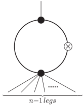
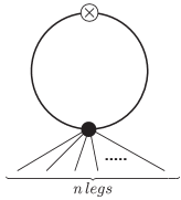
Figure 2: The two diagrams contributing to the flow of the $n$-point vertex and containing vertices with more than $n$ legs.

One can go beyond the leading order approximation, based on eq. (10), in the following way. Focusing on eq. (5) for $\Gamma_{\kappa}^{(2)}(p,-p;\phi)$ one can solve simultaneously the flow equations of $\Gamma_{\kappa}^{(2)}$, $\Gamma_{\kappa}^{(3)}$ and $\Gamma_{\kappa}^{(4)}$, with no approximation in the flow equation for $\Gamma_{\kappa}^{(2)}$, but using (10) in the right-hand-side of the flow equations for $\Gamma_{\kappa}^{(3)}$ and $\Gamma_{\kappa}^{(4)}$. In this way one would determine $\Gamma_{\kappa}^{(3)}$ and $\Gamma_{\kappa}^{(4)}$ with a “leading order” precision and $\Gamma_{\kappa}^{(2)}$ with a “next-to-leading order” one. By iterating the procedure, which amounts to including more equations, one would get better approximations for a larger number of $n$-point functions. It is easily verified that such an iterative approximation scheme reproduces perturbation theory at high momenta: for instance, if the bare vertices of the theory are momentum independent, the leading order approximation contains the exact one loop (this is only true if we keep $q$ in the propagators, as we did in (11)). More generally, a simple analysis shows that to get the expression of a given $n$-point functions at order $m$ loop, one has to consider all equations up to that for the $n+2m-2$-point function. (In a theory with momentum dependent bare vertices, perturbation theory is also reproduced, but more flow equations are required to match perturbation theory at a given number of loops.) Of course, such a scheme is not only accurate at high momenta, where it reproduces perturbation theory, but also in the small momentum, possibly critical, regime, where its accuracy is at least comparable to that of the derivative expansion. In practice, the scheme that we have described may become rapidly cumbersome. However, it can be simplified by using a further approximation consisting in a systematic expansion in $q^{2}/\kappa^{2}$ of the $n$-point functions in the right-hand-side of flow equations. This further approximation preserves the essential property of leading to a closed set of equations. We have solved the flow equation for the 2-point function in leading order and obtained results which are comparable to those obtained in [12]. More complete numerical studies will be presented in a forthcoming publication.

4 The $O(N)$ model in the large $N$ limit

We turn now to the $O(N)$ model in the large $N$ limit, where analytical results can be obtained. Our goal here is twofold. First, to prove that, in its leading order, our approximation is in fact exact in the large $N$ limit. Second, to solve analytically the NPRG equations and find the $n$-point functions in a direct way, i.e., without introducing an auxiliary field, as commonly done [23].

The large $N$ limit of the $O(N)$ model within the NPRG has been thoroughly studied in [24], where it is shown that the effective action takes the form:

$$\Gamma_{\kappa}[\phi]=\int d^{d}x\left\{\frac{1}{2}\partial_{\mu}\phi^{a}\partial_{\mu}\phi^{a}\right\}+\hat{\Gamma}_{\kappa}[\rho],$$ (16)

where $\rho(x)=\phi^{a}(x)\phi^{a}(x)/2$, $a=1,\dots,N$. Using this expression, the authors of Ref. [24] show that the LPA flow equation for the effective potential is exact. Moreover, they find an interesting analytical solution of the equation. However, the use of (16) in the flow equation of a $n$-point function at zero field does not give a closed equation [25]. In this section we obtain a system of closed equations that can be solved analytically.

We shall again focus, for the sake of illustration, on the 2-point function. Its exact flow equation in an external field is the generalization of eq. (5)) to the $O(N)$ model:

$$\partial_{\kappa}\Gamma_{ab}^{(2)}(p,-p;\kappa;\phi) = \int\frac{d^{d}q}{(2\pi)^{d}}\partial_{\kappa}R_{\kappa}(q^{2})\left\{G_{ij}(q^{2};\kappa;\phi)\Gamma_{ajk}^{(3)}(p,q,-p-q;\kappa;\phi)\right.$$ (17)

$$\times G_{kl}((q+p)^{2};\kappa;\phi)\Gamma_{blm}^{(3)}(-p,p+q,-q;\kappa;\phi)G_{mi}(q^{2};\kappa;\phi)$$

$$\left.-\frac{1}{2}G_{ij}(q^{2};\kappa;\phi)\Gamma_{abjk}^{(4)}(p,-p,q,-q;\kappa;\phi)G_{ki}(q^{2};\kappa;\phi)\right\}.$$

At this point, it is useful to recall the structure of the $n$-point functions of the $O(N)$ model in the large N limit. These are obtained by taking the functional derivatives of (16), letting the background field to be constant, and then taking the Fourier transform. We obtain in this way the following expressions for the 2-, 3- and 4-point vertices:

$$\Gamma_{ab}^{(2)}(p,-p;\kappa;\phi)=(p^{2}+V^{\prime}_{\kappa}(\rho))\delta_{ab}+\phi_{a}\phi_{b}\hat{\Gamma}^{(2)}_{\kappa}(p,-p;\rho),$$ (18)

$$\Gamma_{abc}^{(3)}(p_{1},p_{2},p_{3};\kappa;\phi) = \phi_{a}\delta_{bc}\hat{\Gamma}_{\kappa}^{(2)}(p_{1},-p_{1};\rho)+\phi_{b}\delta_{ac}\hat{\Gamma}_{\kappa}^{(2)}(p_{2},-p_{2};\rho)$$ (19)

$$+ \phi_{c}\delta_{ab}\hat{\Gamma}_{\kappa}^{(2)}(p_{3},-p_{3};\rho)+\phi_{a}\phi_{b}\phi_{c}\hat{\Gamma}_{\kappa}^{(3)}(p_{1},p_{2},p_{3};\rho),$$

$$\Gamma_{abcd}^{(4)}(p_{1},p_{2},p_{3},p_{4};\kappa;\phi)=\delta_{ab}\delta_{cd}\hat{\Gamma}_{\kappa}^{(2)}(p_{1}+p_{2},-p_{1}-p_{2};\rho)$$

$$+\delta_{ac}\delta_{bd}\hat{\Gamma}_{\kappa}^{(2)}(p_{1}+p_{3},-p_{1}-p_{3};\rho)+\delta_{ad}\delta_{bc}\hat{\Gamma}_{\kappa}^{(2)}(p_{1}+p_{4},-p_{1}-p_{4};\rho)$$

$$+\delta_{ab}\phi_{c}\phi_{d}\hat{\Gamma}_{\kappa}^{(3)}(p_{1}+p_{2},p_{3},p_{4};\rho)+\delta_{ac}\phi_{b}\phi_{d}\hat{\Gamma}_{\kappa}^{(3)}(p_{1}+p_{3},p_{2},p_{4};\rho)$$

$$+\delta_{ad}\phi_{b}\phi_{c}\hat{\Gamma}_{\kappa}^{(3)}(p_{1}+p_{4},p_{2},p_{3};\rho)+\delta_{bc}\phi_{a}\phi_{d}\hat{\Gamma}_{\kappa}^{(3)}(p_{2}+p_{3},p_{1},p_{4};\rho)$$

$$+\delta_{bd}\phi_{a}\phi_{c}\hat{\Gamma}_{\kappa}^{(3)}(p_{2}+p_{4},p_{1},p_{3};\rho)+\delta_{cd}\phi_{a}\phi_{b}\hat{\Gamma}_{\kappa}^{(3)}(p_{3}+p_{4},p_{1},p_{2};\rho)$$

$$+\phi_{a}\phi_{b}\phi_{c}\phi_{d}\hat{\Gamma}_{\kappa}^{(4)}(p_{1},p_{2},p_{3},p_{4};\rho)\;.$$ (20)

As for the propagator, it can be written in terms of its longitudinal and transverse components:

$$G_{ab}(p^{2};\phi)=G_{T}(p^{2};\rho)\left(\delta_{ab}-\frac{\phi_{a}\phi_{b}}{2\rho}\right)+G_{L}(p^{2};\rho)\frac{\phi_{a}\phi_{b}}{2\rho},$$ (21)

with

$$G_{T}^{-1}(p^{2};\kappa;\rho) = p^{2}+V_{\kappa}^{\prime}(\rho)+R_{\kappa}(p^{2})\;,$$

$$G_{L}^{-1}(p^{2};\kappa;\rho) = p^{2}+V_{\kappa}^{\prime}(\rho)+2\rho\hat{\Gamma}_{\kappa}^{(2)}(p,-p;\rho)+R_{\kappa}(p^{2}).$$ (22)

We can now replace these expressions in eq. (17) and keep only the leading terms in $1/N$. To do so, notice that the non trivial large $N$ limit of the $O(N)$ model is obtained when the effective action $\Gamma_{\kappa}$ is considered to be of order $N$ and the $\phi$ field of order $\sqrt{N}$ (see for example [24]). Then, the 2-point function is of order 1, the 3-point function of order $1/\sqrt{N}$ and the 4-point function of order $1/N$. Simple counting of $N$ factors in the flow equation (17) gives a right hand side of order $1/N$. Thus, the only way of having both sides of order 1 is to collect an explicit $N$ factor from the trace of an identity matrix. The surviving terms yield:

$$\partial_{\kappa}\Gamma_{ab}^{(2)}(p,-p;\kappa;\phi)=N\int\frac{d^{d}q}{(2\pi)^{d}}\partial_{\kappa}R_{\kappa}(q^{2})G_{T}^{2}(q^{2};\kappa;\rho)\left\{-\frac{1}{2}\delta_{ab}\hat{\Gamma}_{\kappa}^{(2)}(0,0;\rho)\right.$$ (23)

$$\qquad\left.+\phi_{a}\phi_{b}\left(\hat{\Gamma}_{\kappa}^{(2)}(p,-p;\rho)\right)^{2}G_{T}((p+q)^{2};\kappa;\rho)-\frac{1}{2}\phi_{a}\phi_{b}\hat{\Gamma}_{\kappa}^{(3)}(p,-p,0;\rho)\right\}.$$

Now comes the important observation: the vertices contributing to the flow in the large-$N$ limit are $q$-independent. That means that our leading order approximation becomes exact in the large-$N$ limit of the $O(N)$ model, as anticipated. Notice that for this to be true, we need to keep the $q$ dependence of the propagators in the flow equations. However, in the large-N limit, the momentum dependence of the transverse propagator (the only one appearing in (23)) is simply the bare one, as shown in eq. (4).

Substituting in eq. (23) the expression (18) of the 2-point function and performing the tensor decomposition, one obtains the system of equations:

$$\partial_{\kappa}V^{\prime}_{\kappa}(\rho) = -\frac{N}{2}V^{\prime\prime}_{\kappa}(\rho)\int\frac{d^{d}q}{(2\pi)^{d}}\partial_{\kappa}R_{\kappa}(q^{2})G_{T}^{2}(q^{2};\kappa;\rho)$$

$$\partial_{\kappa}\hat{\Gamma}_{\kappa}^{(2)}(p,-p;\rho) = N\int\frac{d^{d}q}{(2\pi)^{d}}\partial_{\kappa}R_{\kappa}(q^{2})G_{T}^{2}(q^{2};\kappa;\rho)$$ (24)

$$\times\left\{\left(\hat{\Gamma}_{\kappa}^{(2)}(p,-p;\rho)\right)^{2}G_{T}((p+q)^{2};\kappa;\rho)-\frac{1}{2}\frac{\partial\hat{\Gamma}_{\kappa}^{(2)}(p,-p;\rho)}{\partial\rho}\right\}$$

where we have used, as in eq. (12),

$$\hat{\Gamma}_{\kappa}^{(2)}(0,0;\rho)=V^{\prime\prime}_{\kappa}(\rho),\qquad\hat{\Gamma}_{\kappa}^{(3)}(p,-p,0;\rho)=\frac{\partial\hat{\Gamma}_{\kappa}^{(2)}(p,-p;\rho)}{\partial\rho},$$ (25)

which allowed us to close the equations. In the equations above, $V^{\prime}_{\kappa}(\rho)$ and $V^{\prime\prime}_{\kappa}(\rho)$ denote respectively the first and second derivative of the effective potential with respect to $\rho$.

The first of eqs. (4) is simply the derivative of the equation for the potential in the large-N limit which was solved analytically using two different methods [26, 24]. The second equation, which, to our knowledge, has not been presented before in the literature, can be solved also using any of these two methods. Here we present the solution using the method of [26].

To this aim, we set $W=V^{\prime}_{\kappa}(\rho)$, and use $(\kappa,W)$ as independent variables instead of $(\kappa,\rho)$. In order to do so, we introduce the inverse function relating $\rho$ to $W$:

$$\rho=f_{\kappa}(W)$$ (26)

so that:

$$\partial_{\kappa}f_{\kappa}(W)=-f^{\prime}_{\kappa}(W)\partial_{\kappa}W(\rho),\qquad f^{\prime}_{\kappa}(W)=1/W^{\prime}(\rho),$$ (27)

where $f^{\prime}$ and $W^{\prime}$ are the derivatives of $f$ and $W$ with respect to their respective arguments. Making the change of variables in eq. (4), and using the relations (27), one gets:

$$\partial_{\kappa}f_{\kappa}(W) = \frac{N}{2}\int\frac{d^{d}q}{(2\pi)^{d}}\frac{\partial_{\kappa}R_{\kappa}(q^{2})}{(q^{2}+W+R_{\kappa}(q^{2}))^{2}}$$

$$\partial_{\kappa}\left(\hat{\Gamma}_{\kappa}^{(2)}(p,-p;\rho)\right)^{-1} = -N\int\frac{d^{d}q}{(2\pi)^{d}}\frac{\partial_{\kappa}R_{\kappa}(q^{2})}{(q^{2}+W+R_{\kappa}(q^{2}))^{2}}\frac{1}{(q+p)^{2}+W+R_{\kappa}((q+p)^{2})}$$

At this point we observe that the right hand sides of both the expressions above are total derivatives:

$$\int\frac{d^{d}q}{(2\pi)^{d}}\frac{\partial_{\kappa}R_{\kappa}(q^{2})}{(q^{2}+W+R_{\kappa}(q^{2}))^{2}}=-\partial_{\kappa}\int\frac{d^{d}q}{(2\pi)^{d}}\frac{1}{q^{2}+W+R_{\kappa}(q^{2})}$$

$$\int\frac{d^{d}q}{(2\pi)^{d}}\frac{\partial_{\kappa}R_{\kappa}(q^{2})}{(q^{2}+W+R_{\kappa}(q^{2}))^{2}}\,\frac{1}{(q+p)^{2}+W+R_{\kappa}((q+p)^{2})}$$

$$=-\frac{1}{2}\partial_{\kappa}\int\frac{d^{d}q}{(2\pi)^{d}}\frac{1}{q^{2}+W+R_{\kappa}(q^{2})}\,\frac{1}{(q+p)^{2}+W+R_{\kappa}((q+p)^{2})}.$$

This allows us to integrate analytically the equations. For the potential, one obtains the well known result [26, 5]. By imposing the initial condition that for $\kappa=\Lambda$ the 4-point function is the bare vertex, we get from eq. (4)

$$\hat{\Gamma}_{\kappa=\Lambda}^{(2)}(p,-p;\rho)=\frac{u}{3},$$ (30)

corresponding to a $\phi^{4}$ interaction in the classical action, of the form $(u/4!)(\phi_{a}\phi_{a})^{2}$. We then obtain the longitudinal part of the 2-point function (in the limit $\Lambda\to\infty$):

$$\hat{\Gamma}_{\kappa}^{(2)}(p,-p;\rho)=\frac{u}{3}\frac{1}{1+\frac{Nu}{6}\int\frac{d^{d}q}{(2\pi)^{d}}\frac{1}{q^{2}+W+R_{\kappa}(q^{2})}\frac{1}{(q+p)^{2}+W+R_{\kappa}((q+p)^{2})}}.$$ (31)

This is the usual sum of bubbles in large $N$, which can be found using other methods [23]. Notice however that our solution follows directly from the NPRG without introducing any auxiliary field. The dependence on $W$ reflects the presence of the background field: $W$ plays here the role of a (field dependent) “mass term”.

The same method can be applied to the other $n$-point functions. The calculations are straightforward, but the explicit results involve lengthy expressions. Let us just give here the result for the 3-point function:

$$\hat{\Gamma}^{(3)}_{\kappa}(p_{1},p_{2},p_{3};W) = N\hat{\Gamma}^{(2)}_{\kappa}(p_{1},-p_{1};W)\hat{\Gamma}^{(2)}_{\kappa}(p_{2},-p_{2};W)\hat{\Gamma}^{(2)}_{\kappa}(p_{3},-p_{3};W)$$

$$\times\int\frac{d^{d}q}{(2\pi)^{d}}G_{T}(q^{2};\kappa;\rho)G_{T}((q+p_{1})^{2};\kappa;\rho)G_{T}((q-p_{3})^{2};\kappa;\rho).$$

5 Conclusions and perspectives

In this paper we have presented an approximation scheme to solve the NPRG equations and obtain the $n$-point functions for any external momenta. Our proposal is as general and systematic as the derivative expansion: results can be systematically improved as one can write, at any order, a closed set of equations. We have provided here, as an illustration, an application to the $O(N)$ model in the large $N$ limit: there, the method turns out to be exact at leading order, and it provides an economical procedure to obtain the analytical expressions of the $n$-point functions at arbitrary momenta. Clearly, however, the method is more general. It is based on an approximation that can be exported to other field theories. Work on such extensions, in particular to gauge theories, is underway. This, as well as numerical studies for physically interesting problems, will be reported in forthcoming publications.

References

- [1] N. Tetradis and C. Wetterich, Nucl. Phys. B 422 (1994) 541.
- [2] Ulrich Ellwanger, Z. Phys. C62 (1994) 503–510.
- [3] T. R. Morris, Int. J. Mod. Phys. A9 (1994) 2411–2450.
- [4] T. R. Morris, Phys. Lett. B329 (1994) 241–248.
- [5] J. Berges, N. Tetradis and C. Wetterich, Phys. Rept. 363 (2002) 223–386.
- [6] C Bagnuls and C Bervillier, Phys. Rept. 348(2001) 91.
- [7] B. Delamotte and L. Canet, What can be learnt from the nonperturbative renormalization group?, arXiv:cond-mat/0412205.
- [8] S. Weinberg, Phys. Rev. D8 (1973) 3497.
- [9] U. Ellwanger, Z. Phys., C62 (1994), 503; U. Ellwanger and C. Wetterich, Nucl. Phys. B423 (1994), 137; U. Ellwanger, M. Hirsch and A. Weber, Eur. Phys. J. C 1 (1998) 563; J. M. Pawlowski, D. F. Litim, S. Nedelko and L. von Smekal, Phys. Rev. Lett. 93 (2004) 152002; J. Kato, arXiv:hep-th/0401068; C. S. Fischer and H. Gies, JHEP 0410 (2004) 048.
- [10] For a review, see R. Alkofer and L. von Smekal, Phys. Rep. 353 (2001), 281.
- [11] T. R. Morris, Phys. Lett. B 334 (1994) 355.
- [12] J. P. Blaizot, R. M. Galain and N. Wschebor, Non Perturbative Renormalization Group, momentum dependence of -point functions and the transition temperature of the weakly interacting Bose gas, arXiv:cond-mat/0412481.
- [13] J. P. Blaizot, R. M. Galain and N. Wschebor, A study of the self-energy of the scalar field within the non perturbative renormalization group, in preparation .
- [14] R.D. Ball, P.E. Haagensen, J.I. Latorre, and E. Moreno, Phys. Lett. B347 (1995) 80.
- [15] J. Comellas, Nucl. Phys. B509 (1998) 662.
- [16] D.Litim, Phys. Lett. B486, 92 (2000); Phys. Rev. D64, 105007 (2001); Nucl. Phys. B631, 128 (2002); Int.J.Mod.Phys. A16, 2081 (2001).
- [17] L. Canet, B. Delamotte, D. Mouhanna and J. Vidal. Phys. Rev. D67 (2003) 065004.
- [18] J. Zinn-Justin, Quantum field theory and critical phenomena, Int. Ser. Monogr. Phys. 113 (2002) 1.
- [19] J. Berges, N. Tetradis, and C. Wetterich, Phys. Rev. Lett. 77 (1996) 873–876.
- [20] Daniel F. Litim, Phys. Rev. D64 (2001)105007.
- [21] L. Canet, B. Delamotte, D. Mouhanna and J. Vidal, Phys. Rev. B68 (2003) 064421.
- [22] G. R. Golner, Exact renormalization group flow equations for free energies and N-point functions in uniform external fields, arXiv:hep-th/9801124.
- [23] M. Moshe and J. Zinn-Justin, Phys. Rept. 385, 69 (2003)
- [24] M. D’Attanasio and T. R. Morris, Phys. Lett. B409 (1997) 363–370.
- [25] J.-P. Blaizot, R. Mendez Galain, and N. Wschebor, Non perturbative renormalization group and momentum dependence of -point functions, in preparation.
- [26] N. Tetradis and D. F. Litim, Nucl. Phys. B464 (1996) 492–511.