Cancellation of energy-divergences in Coulomb gauge QCD

Abstract

In the Coulomb gauge of nonabelian gauge theories there are in general, in individual graphs, ‘energy-divergences’ on integrating over the loop energy variable for fixed loop momentum. These divergences are avoided in the Hamiltonian, phase-space formulation. But, even in this formulation, energy-divergences re-appear at 2-loop order. We show in an example how these cancel between graphs as a consequence of Ward identities.

Pacs numbers: 11.15.Bt; 11.10.Gh

Keywords: Coulomb gauge; Renormalization; QCD

1 Introduction

In gauge theories, the Coulomb gauge has special position. The number of dynamical variables is the same as the number of physical degrees of freedom. Moreover, if we go to the Hamiltonian, phase-space, first-order formalism, there are no ghosts; and, because of the existence of a Hamiltonian, unitarity should be manifest.

Nevertheless, there are complications, if not problems, with the Coulomb gauge. In the Lagrangian, second-order, formalism, there are ‘energy-divergences’ in individual Feynman graphs. These are divergences over the energy-integration, $\int dp_{0}$, in a loop, for fixed values of the 3-momentum ${\bf p}$. These are difficult to regularize: dimensional regularization does not touch them, and any other regularization risks doing violence to gauge-invariance (but see Leibbrandt et al for a modified form of dim. reg. [1]). These energy-divergences do cancel when all graphs are combined [2]; but it makes one uneasy to be manipulating divergent and unregulated integrals.

The problem of energy-divergences is eased by going to the Hamiltonian, phase-space, first-order formalism, in which time derivatives of the gluon field ${\bf A}$ are eliminated in favour of the conjugate momentum field ${\bf E}$. This has the advantage of being a true Hamiltonian formalism, and unitarity should be manifestly obeyed. Also, there are no ghosts (ghost loops cancel part of the closed Coulomb loops). For a sample calculation in this formalism see [3], and for possible connection to confinement see [4].

But there are still problems. There is a question of operator-ordering in the Hamiltonian [5] (see also [8], [9]), which may require higher-order terms. It has been shown [6, 7] that these operator-ordering problems are connected with ambiguous multiple energy-integrals in higher orders.

In this paper, we are concerned with a simpler problem, which arises at 2-loop order. In general, in the Hamiltonian formalism to this order, the two integrals over the internal energies converge with the two internal spatial momenta held fixed. However, renormalization demands that we first perform the energy and momentum integrals for each subgraph, then make subtractions for ultraviolet divergences, and then perform the remaining energy and momentum integrals. With this sequence of operations, one does in general find an energy-divergence in the final energy integral.

We illustrate this with a simple example in which quark-loop subgraphs are inserted into the second-order gluon self-energy graphs. We perform the energy-momentum integral in the subgraph first, then do the renormalization subtraction. Individual graphs now have energy-divergences in the final energy integral, but these cancel when graphs are combined. We show that the cancellation is a consequence of the Ward identities obeyed by the quark-loop sub-diagrams.

Of course, it is reassuring to check that the energy-divergences do cancel. But we are back in the uncomfortable position of having to handle divergent (and unregularized) integrals at intermediate stages of the cancellation. This contrasts with the Feynman gauge, where all integrals to all orders are unambiguously regularized by dimensional regularization.

2 Notation, conventions and Feynman rules

Lorentz indices are denoted by Greek letters, spatial indices by $i,j,...$, and colour indices by $a,b,c,...$. We use the metric tensor $g_{{\mu}{\nu}}$, where

$$g_{00}=1,~{}~{}~{}~{}g_{ij}=-\delta_{ij}.$$ (1)

Lorentz vectors are written

$$p=(p_{0};{\bf p}),~{}~{}~{}p^{2}=p_{0}^{2}-{\bf p}^{2}.$$ (2)

We define the Lorentz tensor $G_{{\mu}{\nu}}$ by

$$G_{ij}=g_{ij},~{}~{}~{}G_{0{\mu}}=0,$$ (3)

and for any vector $p_{{\mu}}$ we define the vector $P_{{\mu}}$ by

$$P_{i}=p_{i},~{}~{}~{}P_{0}=0,~{}~{}~{}P^{2}=-{\bf p}^{2}.$$ (4)

(Of course, these definitions refer to the particular time-like vector $(1;0,0,0)$ with respect to which we have chosen to define the Coulomb gauge.) We define a spatial transverse tensor $T$ by

$$T_{{\mu}{\nu}}(p)=-G_{{\mu}{\nu}}+{P_{\mu}P_{\nu}\over P^{2}},$$ (5)

so that

$$T_{ij}(p)=\delta_{ij}-{p_{i}p_{j}\over{\bf p}^{2}},~{}~{}~{}T_{{\mu}0}=0.$$ (6)

In terms of colour matrices $\tau_{a}$, $C_{q}$ is defined by

$$\hbox{tr}(\tau_{a}\tau_{b})=C_{q}\delta_{ab},$$ (7)

and in terms of the structure constants $f_{abc}$, $C_{G}$ is defined by

$$f_{abc}f_{abc^{\prime}}=C_{G}\delta_{cc^{\prime}}.$$ (8)

The renormalized coupling constant is $g$. Quarks have mass $m$.

We use dimensional regularization with spacetime dimension $4-2\epsilon$. The Lagrangian density in the phase-space formalism is

$$L=-{1\over 4}(F^{a}_{ij})^{2}+{1\over 2}(E^{a}_{i})^{2}-E^{a}_{i}F^{a}_{0i}$$ (9)

where

$$E^{a}_{i}F^{a}_{0i}=E^{a}_{i}[\partial_{0}A^{a}_{i}-\partial_{i}A^{a}_{0}-gf^{abc}A^{b}_{0}A^{c}_{i}].$$ (10)

The Hamiltonian form of the Coulomb gauge has dynamical, conjugate fields ${\bf A},{\bf E}$. The Coulomb potential $A_{0}$ is not a dynamical variable. It could be eliminated, but we find it convenient to leave it in the Feynman rules. We use a continuous line to represent ${\bf E}$, a dashed line for ${\bf A}$ and a dotted line for $A_{0}$. The propagators are not diagonal in ${\bf A},{\bf E},A_{0}$. The propagators are shown in Fig.1 (the arrows on the lines show the direction of the momentum $k$). Only one vertex will be relevant to our calculation, that shown in Fig.2.

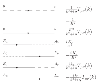
Figure 1: The Feynman rules for propagators in the Hamiltonian Coulomb gauge. Continous lines represent ${\bf E}$, dashed lines ${\bf A}$ and dotted lines $A_{0}$. The arrow indicates the sense of momentum flow.

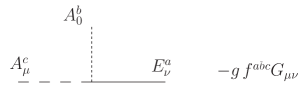
Figure 2: A vertex in the Hamiltonian Coulomb gauge.

Its value is

$$-gf_{abc}G_{{\mu}{\nu}}.$$ (11)

In the Hamiltonian formalism, this is the only vertex involving the Coulomb field. It is this feature which implies there are no energy-divergences to 1-loop order.

3 The quark loop effective action and Ward identities

We are going to insert quark loops into a gluon diagram, so we need a notation for quark 1-loop effective action. Let the 2-gluon term in this effective action be (in momentum space)

$$\delta_{ab}Q_{{\mu}{\nu}}(p)=\delta_{ab}(p^{2}g_{{\mu}{\nu}}-p_{\mu}p_{\nu})Q(p^{2}){(\mu^{2})}^{-\epsilon}.$$ (12)

We will require to know $Q$ only for $~{}~{}|p_{0}|\gg|{\bf p}|,~{}m^{2}.$ In this region, we have

$$Q(p^{2})\sim 8ig^{2}C_{q}\pi^{2-\epsilon}\Gamma(\epsilon){{\Gamma^{2}(2-\epsilon)}\over{\Gamma(4-2\epsilon)}}[(-p_{0}^{2}-i\eta)^{-\epsilon}-(\mu^{2})^{-\epsilon}],$$ (13)

(using minimal subtraction with a mass unit $\mu$).

The 3-gluon term in the effective action will be denoted by

$$if_{abc}\Gamma_{{\mu}{\nu}{\lambda}}(p,q,p^{\prime}),$$ (14)

where $p+q+p^{\prime}=0$, and the quantum numbers of the three gluons are $p,{\mu},a;~{}~{}q,{\nu},b;~{}~{}p^{\prime},{\lambda},c$ (all momenta are directed into the vertex). We will not need to know the value of $\Gamma$ in general. Finally the 4-gluon term in the effective action will be denoted as

$$W^{abcd}_{{\mu}{\nu},{\lambda}{\sigma}}(p,q;k,r),$$ (15)

where the quantum numbers are $p,{\mu},a;~{}~{}q,{\nu},b;~{}~{}k,{\lambda},c;~{}~{}r,{\sigma},d$. Again, we do not need to know the value of $W$ in general. Both $\Gamma$ and $W$ have the symmetries required for Bose symmetry.

Note that the effective action due to quark loops is a functional of $A_{{\mu}}$, and does not depend upon ${\bf E}$. There are terms in the effective action which involve the Coulomb field $A_{0}$, and this is the reason that energy-divergences re-appear. Renormalization requires also the presence of counter-terms with a different structure from the interactions in the original formalism.

The effective action obeys the following Ward identities:

$$p^{{\mu}}\Gamma_{{\mu}{\nu}{\lambda}}(p,q,p^{\prime})=g[Q_{{\nu}{\lambda}}(p^{\prime})-Q_{{\nu}{\lambda}}(q)],$$ (16)

$$p^{{\mu}}W_{{\mu}{\nu}{\lambda}{\sigma}}(p,q;k,r)=-gf_{abe}f_{ecd}\Gamma_{{\nu}{\lambda}{\sigma}}(p+q,k,r)$$

$$-gf_{ace}f_{edb}\Gamma_{{\lambda}{\sigma}{\nu}}(p+k,q,r)-gf_{ade}f_{ebc}\Gamma_{{\sigma}{\nu}{\lambda}}(p+r,q,k).$$ (17)

These identities express the gauge invariance of the quark loop contribution to the effective action. They are a special case of the BRS identities (see for example Itzykson and Zuber equation (12-144)) when there are no ghost contributions [10]. We shall show that these identities are sufficient to ensure the cancellation of energy-divergences between graphs.

4 The energy-divergent graphs

The simplest example of the energy-divergences occurs in the gluon 2-point function, to 2-loop order. The relevant graphs are shown in Fig.3, where the thick circles represent terms from the quark-loop effective action (in (12), (14) and (15)). In Fig.3(vi), the sum of the three subgraphs shown corresponds to (15).

The contributions have the form (in the notation of (4))

$$ig^{2}\delta_{ab}\int d^{4-2\epsilon}p{1\over{P}^{2}}[J^{(i)}_{ij}+J^{(ii)}_{ij}+J^{(iii)}_{ij}+J^{(iv)}_{ij}+J^{(v)}_{ij}+J^{(vi)}_{ij}],$$ (18)

where the roman numbers correspond to the labels on the diagrams.

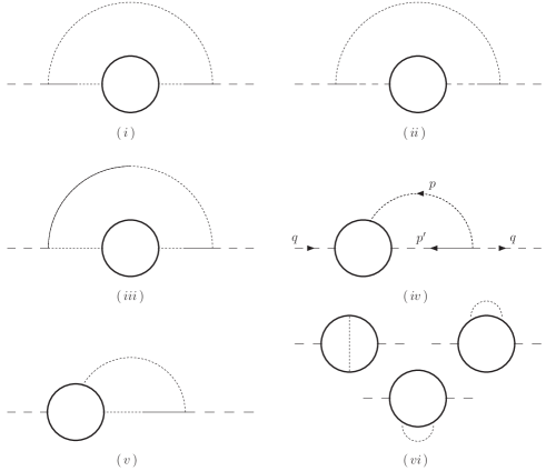
Figure 3: The graphs with energy divergences. The thick black circles represent contributions from quark loops. The other lines are defined in Fig.2.

We have

$$J^{(i)}_{ij}=C_{G}{P^{\prime}_{i}\over P^{\prime 2}}Q_{00}(p^{\prime}){P^{\prime}_{j}\over P^{\prime 2}},$$ (19)

$$J^{(ii)}_{ij}=C_{G}{p^{\prime}_{0}\over p^{\prime 2}+i\eta}T_{i{\mu}}(p^{\prime})Q^{{\mu}{\nu}}(p^{\prime})T_{{\nu}j}(p^{\prime}){p^{\prime}_{0}\over p^{\prime 2}+i\eta},$$ (20)

$$J^{(iii)}_{ij}=-C_{G}{1\over P^{\prime 2}}P_{i}Q_{00}(p^{\prime}){P^{\prime}_{j}\over P^{\prime 2}}+(i\leftrightarrow j),$$ (21)

$$J^{(iv)}_{ij}=C_{G}\Gamma_{i{\mu}0}(q,p^{\prime},p){p^{\prime}_{0}\over p^{\prime 2}+i\eta}T^{{\mu}}_{j}(p^{\prime})+(i\leftrightarrow j),$$ (22)

$$J^{(v)}_{ij}=C_{G}\Gamma_{i00}(q,p^{\prime},p){P^{\prime}_{j}\over P^{\prime 2}}+(i\leftrightarrow j),$$ (23)

$$J^{(vi)}_{ij}={1\over 2}W_{00,ij}(p,q).$$ (24)

The energy-divergences come from the region of integration where

$$p_{0}\gg|{\bf p}|,~{}q_{0},~{}|{\bf q}|,~{}m.$$ (25)

To examine these divergences, we may use in (19), (20) and (21)

$$Q_{00}(p^{\prime})\sim P^{\prime 2}Q(p_{0}),~{}~{}~{}Q_{ij}\sim G_{ij}p_{0}^{2}Q(p_{0}).$$ (26)

We then see that (19), (20) and (21) are each divergent as integrals over $p_{0}$ for fixed ${\bf p}$. (Actually, for $\epsilon>0$ this is true only of the contributon from the subtraction term in (13).) If we take the limit $\epsilon\rightarrow 0$ first, then we get a double log energy-divergence.

To find the behaviour of the integrals in (22), (23) and (24), it is sufficient to use the Ward identities (16) and (17) in the large $p_{0}$ limit. Then (16) gives

$$p_{0}\Gamma_{0ij}(p,q,p^{\prime})\sim gQ_{ij}(p)\sim gG_{ij}(p)p_{0}^{2}Q(p_{0}).$$ (27)

Also,

$$p_{0}^{2}\Gamma_{00i}(p,q,p^{\prime})\sim p^{{\mu}}p^{\prime{\nu}}\Gamma_{{\mu}{\nu}i}-p^{{\mu}}P^{\prime j}\Gamma_{{\mu}ji}-p^{\prime{\nu}}P^{j}\Gamma_{j{\nu}i}$$

$$=-g(P^{j}-P^{\prime j})G_{ij}p_{0}^{2}Q(p_{0})=g(P_{i}-P^{\prime}_{i})p_{0}^{2}Q(p_{0}).$$ (28)

Similarly, (17) implies that

$$p_{0}^{2}W^{aacd}_{00,ij}(p,-p,q,-q)\sim p_{0}gC_{G}\delta_{cd}[\Gamma_{j0i}(p,-p,0)-\Gamma_{ij0}(p,0,-p)]$$

$$\sim 2g^{2}C_{G}G_{ij}(p)p_{0}^{2}Q(p_{0})\delta_{cd},$$ (29)

using (27) again.

From (27), (28) and (29), we see that all the integrals in (18) have energy-divergences of the same kind, and the divergent part has the form

$$ig^{2}C_{G}\delta_{ab}\int d^{3-2\epsilon}{\bf p}{1\over{P^{2}}}dp_{0}Q_{(}p_{0})[K^{(i)}_{ij}+...+K^{(vi)}_{ij}],$$ (30)

where

$$K^{(i)}_{ij}={P^{\prime}_{i}P^{\prime}_{j}\over P^{\prime 2}},$$ (31)

$$K^{(ii)}_{ij}=-T_{ij}(P^{\prime}),$$ (32)

$$K^{(iii)}_{ij}=-{P_{i}P^{\prime}_{j}+P_{j}P^{\prime}_{i}\over P^{\prime 2}},$$ (33)

$$K^{(iv)}_{ij}=2T_{ij}(P^{\prime}),$$ (34)

$$K^{(v)}_{ij}={(P_{i}P^{\prime}_{j}+P_{j}P^{\prime}_{i})\over P^{\prime 2}}-2{{P^{\prime}_{i}P^{\prime}_{j}}\over{P^{\prime 2}}},$$ (35)

$$K^{(vi)}_{ij}=G_{ij}(P^{\prime}).$$ (36)

These last six expressions cancel, so the energy-divergences in the separate terms in (18) cancel out in the sum.

Probably similar cancellations occur in two-loop graphs made entirely of gluon lines. But in this case there is the extra complication of the ambiguous integrals connected to the Christ-Lee terms [6] [7].

Acknowledgement. This work was supported by MZOS of the Republic of Croatia under Contract No. 0098003 (A.A.). We are grateful to Dr. G. Duplančić for drawing the figures.

References

- [1] G. Heinrich and G. Leibbrandt, Nucl. Phys. B 575, 359 (2000)
- [2] R.N. Mohapatra, Phys. Rev. D4 22,378, 1007 (1971)
- [3] A. Andraši, Eur. Phys. J. C 37, 307-313 (2004)
- [4] A. Cucchieri, D. Zwanziger, Phys. Rev. D 65, 014002 (2002)
- [5] N. Christ, T. D. Lee, Phys. Rev. D22, 939 (1980)
- [6] P. Doust, Ann. of Phys. 177, 169 (1987); P. Doust, J. C. Taylor, Phys. Lett. 197, 232 (1987)
- [7] J. C. Taylor, in Physical and Nonstandard Gauges, Proceedings, Vienna, Austria 1989, edited by P. Gaigg, W. Kummer, M. Schweda
- [8] J. Schwinger, Phys. Rev. 127, 234 (1962); Phys. Rev. 130 406 (1963)
- [9] H. Cheng, E. C. Tsai, Phys. Lett. B 176 130 (1986); Phys. Rev. Lett. 57 511 (1986)
- [10] C. Itzykson and J. B. Zuber, Quantum Field Theory, International Series in Pure and Applied Physics, McGraw-Hill Inc. (1980)