On Interpretation of Special Relativity:
a complement to
Covariant Harmonic Oscillator Picture

Abstract

In 1971 Feynman, Kislinger and Ravndal [1] proposed Lorentz-invariant differential equation capable to describe relativistic particle with mass and internal space-time structure. By making use of new variables that differentiate between space-time particle position and its space-time separations, one finds this wave equation to become separable and providing the two kinds of solutions endowed with different physical meanings. The first kind constitutes the running waves that represent Klein-Gordon-like particle. The second kind, widely discussed by Kim and Noz [4], constitutes standing waves which are normalizable space-time wave functions. To fully appreciate how valuable theses solutions are it seems necessarily, however, to verify a general outlook on relativity issue that (still) is in force. It was explained [5] that Lorentz symmetry should be perceived rather as the symmetry of preferred frame quantum description (based on the freedom of choice of comparison scale) than classical Galilean idea realized in a generalized form. Currently we point to some basic consequences that relate to solutions of Feynman equation framed in the new approach. In particular (i) Lorentz symmetry group appears to describe energy-dependent geometry of extended quantum objects instead of relativity of space and time measure, (ii) a new picture of particle-wave duality involving running and standing waves emerges, (iii) space-time localized quantum states are shown to provide a new way of description of particle kinematics, and (iv) proposed by Witten [14] generalized form of Heisenberg uncertainty relation is derived and shown be the integral part of overall non-orthodox approach.

1 Introduction

Since early seventies Kim and Noz [2] proposed unconventional outlook on the issue of relationship between the quantum mechanics and special relativity. Although they did not admit this openly, in fact, they have suggested that special relativity can be understood properly only within the framework of quantum mechanics. In many of his papers Kim pointed out that known aspect of length contraction wins its clarify meaning exclusively against a background of wave description. Such a view allows us to avoid many confusing and misleading interpretations that plague relativity from its very beginning and which cannot be removed if one relays exclusively on the classical approach. As noticed by Kim: “If not possible, it is very difficult to formulate Lorentz boosts for rigid bodies. On the other hand, it seems to be feasible to boost waves” [3].

The author of this paper strongly support the thesis that special relativity is integral part of quantum mechanics and that separation between these two realms is apparent and artificial. Simple analysis given in [5] showed that the source of Lorenz symmetry is not relativity of inertial frames but the freedom of choice of comparison scale imposed on two quantities being given in different physical units (like energy and momentum, and/or distance and time). In particular it was shown that idea of comparison scale combined with two fundamental postulates of quantum mechanics, of  Planck and de Broglie, provides the basis of covariant relativistic description, thereby predicts basic dynamical features of relativistic particles. It was explained also that Lorentz symmetry needs to be seen as the symmetry of preferred frame (i.e. observer rest frame) quantum description. In this paper we continue the progress along that line by indicating that Lorentz symmetry group is a natural tool to describe internal space-time structure of extended quantum objects. Discussed in the paper the main consequences resulting from such non-orthodox point of view are:

1. The time and length measure relativity aspect is taken over by issue of energy-dependent space-time deformation of extended quantum objects.

2. Space-time localized quantum states are shown to provide a new way of description of particle kinematics.

3. A new picture of particle-wave duality involving running and standing waves becomes visible.

The solutions of covariant harmonic oscillator equation provided by Kim and Noz [4] state plausible illustration for the presented ideas.

The structure of the paper is the following: In Section 2 we start with a pure quantum-mechanical analysis intended to recollect the way which two light-cone momenta put together may constitute a four-momentum of relativistic particle with mass. Then we introduce a concept of light-cone skeleton, which will enable us to link particle dynamical features with its space-time extensions and thus with its kinematical properties. The differential equation of Feynman, Kislinger and Ravndal [1], i.e. the covariant harmonic oscillator equation, as well as, the basic properties of solutions of this equation obtained by Kim and Noz are discussed in Section 3. We show/recollect also the way which scalar particle gains its mass due to vibrations of its internal space-time structure and analyze the particle ground state geometry. The light-cone skeleton structure, introduced in Section 2, turns out to be a useful quantum-mechanical tool to characterize excitation levels of extended oscillatory particle. The two kinds of such excitations, called respectively kinetic and potential are distinguished and described in Section 4. Both of them are shown to be space-time localized but their physical meanings differ. The kinetic excitations are identified with four-momentum transfer carried out by running plane-waves embraced, however, within a space-time localized area which extensions are determined just by the light-cone skeleton structure. On the other hand, the same light-cone structure is shown to spread out the potential excitations formed by standing waves. A new picture of particle-wave duality expressed in terms of kinetic and potential excitations is the subject of Section 5. The issue of oscillatory motion of extended quantum object is discussed next. The energy and momentum fluctuations that relate to this peculiar kind of motion are shown to be in Heisenberg-Witten relation which is a generalized form of Heisenberg uncertainty relation proposed by Witten [14]. Finally, in Section 6, we recollect some experimental results that in spectacular manner disclose non-locality of quantum mechanics.

2 Quantum-mechanical description of relativistic particle with mass

The Klein-Gordon equation for scalar particle or the Dirac equation for spin-half particle are the basic tools of relativistic quantum field theory that make descriptions of massive particles possible. Nevertheless, the introduction of particle mass in the relativistic case, similarly like in the non-relativistic case of Schrödinger quantum mechanics, is equivalent to introduction of mass parameter. Since each of the mentioned wave equations cannot predict itself possible particle internal space-time structure, it is widely believed that point-particle picture is the most accurate one.

Conventional field theory methods, however, indicates also another, quite different way of mass introduction. A very instructive example provides us the solutions of covariant harmonic oscillator equation given by Kim and Noz [4]. Their analysis is complete and thorough. They showed that emerging particle picture is not point-like but takes the form of extended quantum object which internal space-time structure is characterized by Wigner’s O(3)-little group. Another consequence resulting from Kim and Noz solutions is that particle mass (or rather the mass of extended quantum object) is generated by oscillatory-like field vibrations.

The purpose of this section is to describe simply quantum-mechanical structure, called further the light-cone skeleton, that underlies the solutions of relativistic oscillator equation. In particular this quantum-mechanical structure turns out to be very useful to show the way which particle internal space-time structure becomes energy-dependent, as well as, the way which particle motion can be expressed in terms of space-time localized quantum states.

2.1 Composite structure of massive state

It was shown [5] that four-momentum of relativistic particle with mass can be made up of two light-cone momenta of massless particles. Since each of the vectors of Minkowski space can be given in form of two superposed light cone vectors, from the algebraic point of view, of course, there is no surprise. The key point is, however, that in the case of on-mass-shell four-momentum the magnitudes of these two light-cone momenta are related through the scaling symmetry [5]. This property is most easily observed in $1+1$ dimensional gauge frame. Let us then recollect that introduced in [5] gauge frame was called the frame at which momentum (or space) axis was chosen such to match the direction of particle motion. The gauge frame description may then reduce the four-momentum to bi-momentum one.

So, let us consider a bimomentum $\binom{\Pi_{0}}{\Pi_{1}}$ given at the photonic frame (i.e. the frame which axes considered at the Minkowski gauge frame are the light-cone axes) and assume that

$$\left(\begin{array}[c]{c}\Pi_{0}\\ \Pi_{1}\end{array}\right)=\left(\begin{array}[c]{cc}\frac{1}{\eta}&0\\ 0&\eta\end{array}\right)\binom{\frac{m_{0}c}{\sqrt{2}}}{-\frac{m_{0}c}{\sqrt{2}}},$$ (1)

describes a relativistic particle with mass $m_{0}$. Indeed, at the Minkowski gauge frame $\binom{\Pi_{0}}{\Pi_{1}}\rightarrow\binom{P_{0}}{P_{1}}$ where

$$\left(\begin{array}[c]{c}P_{0}\\ P_{1}\end{array}\right)=\left(\begin{array}[c]{cc}\frac{1}{\sqrt{2}}&\frac{-1}{\sqrt{2}}\\ \frac{1}{\sqrt{2}}&\frac{1}{\sqrt{2}}\end{array}\right)\left(\begin{array}[c]{c}\Pi_{0}\\ \Pi_{1}\end{array}\right),$$ (2)

one finds that

$$\left(\begin{array}[c]{c}P_{0}\\ P_{1}\end{array}\right)=\left(\begin{array}[c]{c}\gamma m_{0}c\\ -\gamma\beta m_{0}c\end{array}\right),$$ (3)

where

$$\gamma=cosh\xi\text{ \ \ \ and \ \ \ }\gamma\cdot\beta=sinh\xi,$$ (4)

for $\xi=ln\eta.$ Decomposition of Minkowski bi-momentum (3) at the photonic frame was shown on Fig.1.

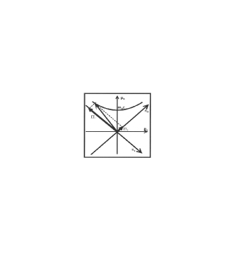
Figure 1: Decomposition of Minkowski four-momentum in the photonic frame. The amplitudes of light-cone vectors $\Pi_{0}$ and $\Pi_{1}$ are related through the scaling factor $\eta$, namely: $\Pi_{0}=\frac{1}{\eta}\frac{m_{0}c}{\sqrt{2}}$ and $\Pi_{1}=\eta\frac{m_{0}c}{\sqrt{2}}.$

The question one may ask, however, is whether the orthogonal transformation (2) is only an alternative of bi-momentum expression, or it reveals also a composite structure of a massive state. Note, that following two bi-momenta $\binom{\Pi_{0}}{0}$ and $\binom{0}{-\Pi_{0}}$ given at the photonic frame, at the Minkowski gauge frame turn into $\binom{\Pi_{0}/\sqrt{2}}{\Pi_{0}/\sqrt{2}}$ and $\binom{\Pi_{0}/\sqrt{2}}{-\Pi_{0}/\sqrt{2}},$ which describe two photon states having opposite momenta, thereby opposite propagation directions. A possibility of expression of massive state in terms of two massless excitations propagating the opposite way rises, however, another essential question, namely, how to explain that two such excitations can describe a particle movement at all. The next two subsections are aimed to approach to these issues in the most elementary way.

2.2 Idea of light-cone skeleton

A natural consequence of the assumption about composite particle structure must be departure from point-particle picture. It is widely believed that such departure has been already done in terms of wave packet description, which is basically true. Nevertheless, the point-particle picture still remains valid as the classical one. Therefore, to emphasize the difference between point-particle and extended object conceptual views we introduce the idea of light-cone skeleton intended to describe internal space-time structure of particle with mass. As pointed out, the idea of light-cone skeleton is purely quantum-mechanical one, thus, if correct, it should play a similar role in field theory approach as the postulates of Planck and de Broglie do in Schrödinger theory.

In order to introduce extended quantum object description we start with generic example of circle of radius $\lambda_{C}/2$ centered at the origin of photonic (or Minkowski gauge) frame, as shown on Fig.2a, and assume that this circle embraces a space-time area where extended quantum object is localized. In terms of wave description one may expect this area to indicate the maximum of probability density of quantum object distribution. Let us assume also that the geometry of considering space-time region is the ground state geometry, thereby the geometry of extended quantum object at rest (this assumption is to become clear later).

Figure 2: Boost deformation of extended quantum object. (a) The circle represents space-time area of quantum object staying at rest. (b) At higher (kinetic) energy level extended quantum object become localized at space-time elliptical region. The vectors $\Lambda_{1}$ and $\Lambda_{2}$ were called the light-cone skeleton. The boost transformation then corresponds to light-cone skeleton deformation described by Eq. 8. Presented figure (almost) is reprinted from [4].

Next, let us consider another space-time area, now taking the form of an ellipse (i.e. a deformed circle), as shown on Fig.2b, and assume that it describes the same quantum object but already at a higher energy level. Let as assume also that this higher energy level (established at the observer rest frame) corresponds to an excited particle state that relates to particle motion (i.e. the motion which is observed at the observer rest frame too). The two light cone vectors $\Lambda_{0}$ and $\Lambda_{1},$ which, as it comes from Fig.2b, “spreads out” the ellipse along its major and minor axes, will be called further the light-cone skeleton.

Although there is no need to assign any special value to $\lambda_{C}$ , and thus to $\Lambda_{0}$ and $\Lambda_{1}$, for illustrative purpose it is advisable to consider a particle of model shape. Model shape particle will be called the particle which light-cone skeleton extensions $\lambda_{0}$ and $\lambda_{1}$, as depicted on Fig.3, are de Broglie wavelengths of light-cone momenta (1). The extensions of model shape particle then are directly related to its dynamical features according to

$$\Pi_{0}=\frac{h}{\lambda_{0}}\text{ \ \ \ and \ \ }\Pi_{1}=-\frac{h}{\lambda_{1}}.$$ (5)

So, the light-cone skeleton for particle of model shape is

$$\left(\begin{array}[c]{c}\Lambda_{0}\\ \Lambda_{1}\end{array}\right)=\left(\begin{array}[c]{c}\frac{1}{2}\lambda_{0}\\ \frac{1}{2}\lambda_{1}\end{array}\right)=\left(\begin{array}[c]{c}\frac{1}{2}\frac{1}{\sqrt{2}}\eta\lambda_{C}\\ \frac{1}{2}\frac{1}{\sqrt{2}}\frac{1}{\eta}\lambda_{C}\end{array}\right),$$ (6)

where, due to (1)

$$\lambda_{C}=\frac{h}{m_{0}c},$$ (7)

is the Compton wavelength.

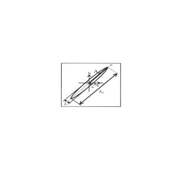
Figure 3: The particle of “model shape”. The light-cone skeleton extensions of particle of model shape, $\lambda_{0}$ and $\lambda_{1}$, correspond exactly to its energy and momentum, see formulas (2), (3) and (5).

The light-cone skeleton structure then links particle dynamical and geometrical properties. Indeed, one easily finds that there is $1:1$ correspondence between particle dynamical features expressed in terms of light-cone momenta (1) and $circle\rightarrow ellipse$ transition described by light-cone skeleton deformation

$$\left(\begin{array}[c]{c}\Lambda_{C}\\ \Lambda_{C}\end{array}\right)\rightarrow\left(\begin{array}[c]{c}\Lambda_{0}\\ \Lambda_{1}\end{array}\right)=\left(\begin{array}[c]{c}\eta\Lambda_{C}\\ \frac{1}{\eta}\Lambda_{C}\end{array}\right),$$ (8)

where, due to (6), $\Lambda_{C}=\lambda_{C}/2\sqrt{2}$ (cf. Fig.2). So, one finds that along with particle (kinetic) energy increase the area of its space-time localization becomes more and more elongated [12]. Such behavior, of course, is unpredictable within the framework of Schrödinger quantum mechanics. On the other hand, it becomes visible that special relativity put in “exclusive hands of quantum mechanics” must provide a description of particle motion quite different from that, which by making use of classical approach, we get used to it.

2.3 Moving particle and space-time localized quantum states

Particle kinematics expressed in terms of space-time localized quantum states naturally blends into the landscape of quantum mechanics based on the ground of the covariant and preferred frame description. In such environment difficulties related to time and length measure do not even have a chance to appear, so that the relativity issue becomes ripped its “mystery cover” off. One of the consequence resulting from that is that relativity aspect is fund to provide a number interesting insights about internal particle space-time structure. Given that we do have a relativistic wave equation that yield space-time localized solutions, let us try to draw some basic conclusions resulting from that.

To apply the earlier results let us consider a particle of model shape which ground state probability distribution is centered in circle of radius $\lambda_{C}/2.$ In such case, as noticed, the particle must stay at rest, so that its Minkowski frame bi-momentum $\binom{P_{0}}{P_{1}}=\binom{m_{0}c}{0}.$ Along with particle energy increase its space-time structure is supposed to become changed as well. Indeed, the boost transformation that induces $\binom{m_{0}c}{0}\rightarrow\binom{\gamma m_{0}c}{\gamma\beta m_{0}c},$ must affect also the light-cone skeleton structure, thereby the geometry of the state. Due to (8), the circle area of ground state must be transformed into elliptical region of excited state. Let us then explain the way which light-cone skeleton deformation shown on Fig.2 provide informations about particle kinematics.

For that purpose, let us assume that effectively measured quantities at the real space are not the light-cone ones but, similarly like in the case of bi-momentum (2), are the corresponding to them Minkowski “equivalents”. Thus, the relationship between the Minkowski intervals and space-time separations of quantum object expressed via light-cone skeleton structure, as shown on Fig.4a, are

$$\left(\begin{array}[c]{c}\frac{\Delta x_{0}}{2}\\ \frac{\Delta x_{1}}{2}\end{array}\right)=\left(\begin{array}[c]{cc}\frac{1}{\sqrt{2}}&\frac{1}{\sqrt{2}}\\ -\frac{1}{\sqrt{2}}&\frac{1}{\sqrt{2}}\end{array}\right)\left(\begin{array}[c]{c}\Lambda_{1}\\ \Lambda_{2}\end{array}\right).$$ (9)

The physical meaning of intervals $\Delta x_{0}$ and $\Delta x_{1}$ seems to be complementary. Indeed, by making use of textbook formulas which allow us to combine scaling parameter $\eta$ (see (4)) with a velocity $w$ according to

$$\gamma=\frac{1}{\sqrt{1-w^{2}/c^{2}}}\text{ \ and \ }\beta=\frac{w}{c},$$ (10)

one obtains

$$\Delta x_{0}=\frac{1}{\sqrt{1-w^{2}/c^{2}}}\lambda_{C},$$ (11)

and

$$\Delta x_{1}=\frac{w/c}{\sqrt{1-w^{2}/c^{2}}}\lambda_{C}\text{\ .}$$ (12)

Note, that $\Delta x_{0}\geqslant\Delta x_{1}.$ In particular, for $w$ $\lessapprox$ $c,$ the both intervals are almost equal, but in the case of $w=0$, $\Delta x_{0}=\lambda_{C}$ whereas $\Delta x_{1}=0.$ This suggests that $\Delta x_{1}$ may be understood as the uncertainty of particle center (of mass) position inside some “quantum region”, in time period resulting just from (11). Thus, one may say that uncertainty $\Delta x_{1}$ applies to point-particle position indeed. Assuming that this point-particle moves (or oscillates) inside the mentioned quantum area, one may call such movement a movement in a classical channel. On the other hand, time separation $\Delta x_{0}$ might be identified with the time of life of temporarily localized quantum state (do not mistake with particle life time), which classical channel width (or uncertainty) is just $\Delta x_{1}.$ Thus, the time separation interval $\Delta x_{0}$ might be called the uncertainty of quantum channel.

Figure 4: Two mutually conjugated light-cone structures given respectively in position and momentum space. (a) The space-time area “spread out” on light-cone skeleton structure in position space indicates maximum probability density of quantum object distribution. One the other hand the very light cone skeleton extensions projected on Minkowski frame axes provide informations about particle kinematics (see formula (9)). Similarly, the light-cone skeleton structure given in momentum space (b) determines energy-momentum distribution of extended quantum object [4]. For the particle of model shape its energy and momentum fluctuations amount to its energy and momentum themselves (see formula (58)).

To find the explicit dependence between the life times of quantum state of moving particle and particle at rest, let as put

$$\lambda_{C}=c\Delta\tau\text{ \ \ and \ \ }\Delta x_{0}=c\Delta t,$$ (13)

which means that intervals $\Delta\tau$ and $\Delta t$ are respectively the time separations of ground state and excited state of particle motion. Then, by combining formula (13) with (11) and (12) one obtains the following expressions

$$\Delta t=\frac{\Delta\tau}{\sqrt{1-w^{2}/c^{2}}},$$ (14)

and

$$\Delta x_{1}=w\Delta t,$$ (15)

which explain, so-called, time dilatation effect, now in pure quantum-mechanical manner. It is clear that currently formula (14) has noting to do with “relativistic time measure”. Instead, one finds that the task of this “relativistic effect” is taken over by energy-dependent deformation of particle internal space-time structure.

Description of particle motion based on temporarily localized quantum states distinguishes the following two situations: the first one is when particle life-time and the life-time of temporarily localized quantum state are the same, and the second one is when particle life-time is substantially longer. So, in the latter case the quantum picture of particle motion cannot be given in a form of single space-time localized region, as shown on Fig.4a, but it must consist of many such regions, as shown on Fig.5. The particle motion then cannot be considered smooth, but rather as a jump-like or oscillatory motion. The analysis of covariant harmonic oscillator solutions will bring us to this point again later on.

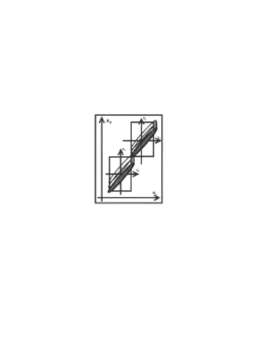
Figure 5: Oscillatory motion of extended quantum object. The motion induced by kinetic and potential excitations (described in Section 5) effectively takes the form of space-time probability current flow.

And finally, let us note that formulas (11), (12) and (7) enable us to express particle space-time extensions in form of Lorentz invariant interval

$$\left(\Delta x_{0}\right)^{2}-\left(\Delta x_{1}\right)^{2}=\left(\frac{h}{m_{0}c}\right)^{2}.$$ (16)

which, in clear-cut way, points out to the relationship between the special relativity and quantum mechanics.

3 Wave description of extended quantum object

Relativistic oscillator wave function has been considered already by Yukawa in 1953 [6] who attempted to model the behavior of relativistic particles having internal structures. Later this issue also was undertaken by Feynman [1] who paradoxically suggested himself to use relativistic oscillator wave functions instead of his diagrams for study hadronic structures and interactions. Nevertheless, the powerful method of Feynman diagrams has effectively overshadowed many interesting results of bound states analysis carried out strictly within the boundaries of covariant approach.

The main purpose of this section is to show that Feynman equation equipped with Kim and Noz solutions provides two seemingly quite different particle images. The first point-particle image is associated with running waves (and thus with underlaying structure of Feynman diagrams). The other particle image emerges from normalizable wave functions and takes the form of extended quantum object.

3.1 Feynman equation and Kim and Noz solutions

The differential equation of Feynman, Kislinger and Ravndal [1], namely

$$\left\{\left[\left(\frac{\partial}{\partial x_{a}^{\mu}}\right)^{2}+\left(\frac{\partial}{\partial x_{b}^{\mu}}\right)^{2}\right]-\frac{\kappa}{8}\left(x_{a}^{\mu}-x_{b}^{\mu}\right)^{2}\right\}\phi(x_{a,}x_{b})=0,$$ (17)

was aimed to describe a hadron consisting of two quarks at $x_{a}$ and $x_{b},$ bound together by a harmonic oscillator potential of strength $\kappa$. Actually, Eq. (17) is the Kim and Noz version of Feynman equation [4], where, additionally, the potential constant $\kappa,$ now, is kept in the explicit form to emphasize the meaning of units of $\kappa=1$ later on. Furthermore, since the algebraic structure of quarks is not taken into account, it is enough to assume that $x_{a}$ and $x_{b}$ are the coordinates of self-interacting scalar quantum object.

Following the procedure of Kim and Noz let us introduce the new variables:

$$X=\frac{x_{a}+x_{b}}{2},$$ (18)

which specifies the quantum object space-time position and

$$x=\frac{x_{a}-x_{b}}{2},$$ (19)

which determines quantum object space-time separations. The new variables make possible to write down Eq. (17) in explicitly separable form

$$\left\{\left(\frac{\partial}{\partial X^{\mu}}\right)^{2}+\left[\left(\frac{\partial}{\partial x^{\mu}}\right)^{2}-\kappa\left(x^{\mu}\right)^{2}\right]\right\}\phi(X,x)=0.$$ (20)

Indeed for

$$\phi(X,x)=f(X)\cdot\psi(x),$$ (21)

one finds that following two differential equations must be satisfied:

$$\left\{\left(\frac{\partial}{\partial X^{\mu}}\right)^{2}+\left(\frac{Mc}{h}\right)^{2}\right\}f(X)=0,$$ (22)

and

$$\left[\left(\frac{\partial}{\partial x^{\mu}}\right)^{2}-\kappa\left(x^{\mu}\right)^{2}\right]\psi(x)=\left(\frac{Mc}{h}\right)^{2}\psi(x).$$ (23)

Equation (22) is a Klein-Gordon equation for particle with mass $M$. The solutions of this equation are the plane waves

$$\ f(X)=f_{0}e^{\pm\left(P\nu X^{\nu}\right)},$$ (24)

which, indeed, call the image of point-particle carrying out the four-momentum $P_{\nu},$ where $P_{\nu}P^{\nu}=M^{2}c^{2}.$ Currently, however, relativistic particle is described also by Eq. (23). But Eq. (23) determines not only the value of particle mass, but also it dresses it up with internal space-time structure. To observe this, as well as, because of the fact that solutions of (23) are naturally given in dimensionless units, it is advisable to write down Eqs. (22) and (23) in reduced form. For that purpose let us introduce some characteristic length scale $\lambda_{c}/2$ and rewrite Eq. (22) as

$$\left\{\left(\frac{\partial}{\partial\widetilde{X}^{\nu}}\right)^{2}+\mu^{2}\right\}f(\widetilde{X})=0,$$ (25)

where $\widetilde{X}^{\nu}=\frac{X^{\nu}}{\lambda_{c}/2},$

$$f(\widetilde{X})=f_{0}e^{\pm\left(\widetilde{P}\nu\widetilde{X}^{\nu}\right)},$$ (26)

so that

$$\widetilde{P}\nu\widetilde{P}^{\nu}=\mu^{2}.$$ (27)

Similarly, in the case of Eq. (23) one obtains

$$\left[\left(\frac{\partial}{\partial\widetilde{x}^{\mu}}\right)^{2}-\kappa\left(\frac{\lambda_{c}}{2}\right)^{4}\left(\widetilde{x}^{\mu}\right)^{2}\right]\psi(\widetilde{x})=\mu^{2}\psi(\widetilde{x}),$$ (28)

where $\widetilde{x}^{\mu}=\frac{x^{\mu}}{\lambda_{c}/2}.$ Additionally, if one puts

$$\kappa\left(\frac{\lambda_{c}}{2}\right)^{4}=1,$$ (29)

one finds that notation that involves unit potential strength makes use of intrinsically built in length scale $\lambda_{c}$. Elementary solution of Eq. (20) is then a plane wave $f(\widetilde{X})$ which amplitude is localized in some space-time region, if only $\psi(\widetilde{x})$ is entirely normalizable function.

To find the solutions of Eq. (28) let us assume that condition (29) is fulfilled and (by skipping the tildes from now on) let us rewrite this equation in more explicit form

$$\left[\left(\frac{\partial^{2}}{\partial x_{0}^{2}}-\frac{\partial^{2}}{\partial\mathbf{x}^{2}}\right)+\left(x_{0}^{2}-\mathbf{x}^{2}\right)\right]\psi_{\lambda}(x)=\mu^{2}\psi_{\lambda}(x).$$ (30)

Eq. (30) was just the starting point of Kim and Noz analysis [4]. They considered next the set of following solutions

$$\psi_{\lambda}(x) =\left(\frac{1}{\pi^{1/4}}\right)^{4}\left(\frac{1}{2}\right)^{(k+l+m+n)/2}\left(\frac{1}{k!l!m!n!}\right)^{1/2}$$ (31)

$$\times H_{k}(x_{0})H_{l}(x_{1})H_{m}(x_{2})H_{n}(x_{3})$$

$$\times exp\left(-\frac{1}{2}\left(x_{0}^{2}+x_{1}^{2}+x_{2}^{2}+x_{3}^{2}\right)\right),$$

where $H_{k}(x_{0}),$ $H_{l}(x_{1})...$ are the Hermite polynomials and the eigenvalue

$$\mu^{2}=1+l+m+n-k\equiv 1+\lambda,$$ (32)

so that $\lambda=l+m+n+k$ where $k,l,m$ and $n$ are integer numbers. So, indeed the wave functions $\psi_{\lambda}(x)$ are entirely normalizable, however, the covariant oscillator problem turns out to be infinitely degenerated. To limit the degeneracy to a finite number, as well as, to retain only those solutions endowed with transparent physical meaning, Kim and Noz imposed a covariant condition that suppressed the time-like oscillations, thereby avoided the problem of negative energies too. The wave function (31) then has been reduced to

$$\psi_{\lambda^{\prime}}(x) =\left(\frac{1}{\pi^{1/4}}\right)^{4}\left(\frac{1}{2}\right)^{(l+m+n)/2}\left(\frac{1}{l!m!n!}\right)^{1/2}$$ (33)

$$\times H_{l}(x_{1})H_{m}(x_{2})H_{n}(x_{3})$$

$$\times exp\left(-\frac{1}{2}\left(x_{0}^{2}+x_{1}^{2}+x_{2}^{2}+x_{3}^{2}\right)\right),$$

where

$$\lambda^{\prime}=l+m+n.$$ (34)

Kim and Noz showed that wave functions (31) constitute irreducible, infinite-dimensional unitary representation of the Lorentz group which describes Klein-Gordon-like particles with definite momentum $P_{\mu}$ and internal space-time structure but devoid of time-like oscillations. We will make use of this crucial property later on. First, however, it is advisable to extract a physical content of solutions (26) and (33) and correlate the “shape” of particle internal structure with its four-momentum $\widetilde{P}_{\mu}$ .

3.2 Geometry of the ground state

Kim and Noz showed that wave functions (31) form a vector space for O(3)-like little group. However, the symmetry of very ground state ($l=m=n=0$),

$$\psi_{0}(x)=\frac{1}{\pi}exp\left(-\frac{1}{2}\left(x_{0}^{2}+x_{1}^{2}+x_{2}^{2}+x_{3}^{2}\right)\right),$$ (35)

turns out even to be the symmetry of four-dimensional sphere. Keeping in mind that function (35) is given in $\lambda_{c}/2$ units, one finds that the radius of “ground state sphere” is $1/\sqrt{2}$ . Indeed, since the ground state function (35) separates according to

$$\psi_{0}(x)=\frac{e^{-\frac{\chi_{0}^{2}}{2}}}{\pi^{1/4}}\frac{e^{-\frac{\chi_{1}^{2}}{2}}}{\pi^{1/4}}\frac{e^{-\frac{\chi_{2}^{2}}{2}}}{\pi^{1/4}}\frac{e^{-\frac{\chi_{3}^{2}}{2}}}{\pi^{1/4}},$$ (36)

the same concerns the probability density distribution

$$\left|\psi_{0}(x)\right|^{2}=\frac{e^{-x_{0}^{2}}}{\pi^{1/2}}\frac{e^{-x_{1}^{2}}}{\pi^{1/2}}\frac{e^{-x_{2}^{2}}}{\pi^{1/2}}\frac{e^{-x_{3}^{2}}}{\pi^{1/2}},$$ (37)

where each of the factors appear to be the Gaussian distributions of the same dispersion $2\sigma=\sqrt{2}$. Thus, if one intersect the sphere $x_{0}^{2}+x_{1}^{2}+x_{2}^{2}+x_{3}^{2}=\frac{1}{2}$ with e.g. $x_{0}x_{1}$ plane one finds that included at this plane light-cone skeleton of coordinates $\binom{1/\sqrt{2}}{1/\sqrt{2}}$ (cf. Fig.2a) becomes representative for the whole quantum object described by Eq. (36). Indeed, accordingly to (9) the light-cone skeleton structure with equal “arms” must describe quantum object at rest. Note also that the form of wave function (36) is invariant with respect to transformation

$$\left(\begin{array}[c]{c}\chi_{0}\\ \chi_{1}\end{array}\right)=\left(\begin{array}[c]{cc}\frac{1}{\sqrt{2}}&\frac{1}{\sqrt{2}}\\ \frac{-1}{\sqrt{2}}&\frac{1}{\sqrt{2}}\end{array}\right)\left(\begin{array}[c]{c}x_{0}\\ x_{1}\end{array}\right),$$ (38)

which replaces the coordinates of Minkowski frame $x_{0},x_{1},$ with those of photonic (or light-cone) ones $\chi_{0},\chi_{1}$. Indeed, since

$$\chi_{0}^{2}+\chi_{1}^{2}=x_{0}^{2}+x_{1}^{2},$$ (39)

alternative form of wave function (36) is

$$\psi_{0}(x,\chi)=\frac{e^{-\frac{\chi_{0}^{2}}{2}}}{\pi^{1/4}}\frac{e^{-\frac{\chi_{1}^{2}}{2}}}{\pi^{1/4}}\frac{e^{-\frac{x_{2}^{2}}{2}}}{\pi^{1/4}}\frac{e^{-\frac{x_{3}^{2}}{2}}}{\pi^{1/4}}.$$ (40)

High symmetry of the ground state makes then that distinction between the coordinates of Minkowski and photonic frames is covered.

In the next section we will show that images of point-particle and extended-particle outlined above are indeed complementary. The light-cone skeleton concept will make us possible to superimpose the both particle pictures. Furthermore, we will indicate the way which particle motion can be described in terms of space-time localized wave packets. So, the issue of normalizable space-time solutions becomes of special interest especially in the context of currently lunching idea that special relativity and quantum mechanic make an indivisible whole.

4 Localized states of motion

Currently discussed approach making the special relativity basically a quantum mechanics toll, enormously simplifies the whole “relativity” issue. Lorentz symmetry becomes no longer identified with the relative motion of inertial frames, thereby the relativity aspect of length and time measure becomes completely withdrawn from the relativity issue along with its orthodox mode. Instead, Lorentz symmetry group turns out to tackle the problem of description of energy-dependent geometry of extended quantum objects.

It was shown [5] that quantum-mechanical symmetry related to the freedom of choice of comparison scale combined with Euclidean rotations led to the concept of Lorentz group. The covariant form of differential equations encompasses then the symmetries of scaling and $3d$ rotations. From the physical point of view, however, more important seem to be the conclusions resulting form solutions of these equations. Given that one really has the solutions that describe quantum object internal space-time structure, the Lorentz group then is expected to disclose many interesting particle features. In this section we make use of Kim and Noz solutions to indicate the way which space-time localized quantum states tackle description of particle motion. The analysis corresponds well to this given in section 2.3, but now, of course, goes much beyond the pure quantum-mechanical considerations.

4.1 Kinetic excitations

Basing on the results of preceding section one finds that complete wave function of the ground state of Eq. (20) is

$$\phi_{0}(X,x)=e^{\pm m_{0}cX^{0}}\cdot\frac{1}{\pi}e^{-\frac{1}{2}\left(x_{0}^{2}+x_{1}^{2}+x_{2}^{2}+x_{3}^{2}\right)}.$$ (41)

(Note that energy $E=m_{0}c^{2}=hc/\lambda_{C}$ corresponds to $\mu=1,$ i.e. the energy expressed in $\lambda_{C}/2$ units). The wave function (41) describes then a relativistic scalar at rest.

The form of wave function (21), or (41), suggests that solutions of relativistic oscillator equation involves two kinds of excitations. The first kind is related to, let say, potential excitations, i.e. excitations induced by vibrations of particle internal structure. According to (27) and (32) one finds that potential excitations are to be characterized by different mass levels.

Another kind of excitations, which, as it comes also from analysis before, is expected to be related directly to particle kinematics. Let us call this kind of excitations the kinetic excitations. In fact the very approach based on preferred frame description invokes the space-time localized quantum states to be the states of particle motion. Let us then determine the notion of  “kinetic excitations” in more precise manner.

The simplest and most natural way to obtain the state of particle motion is to boost the ground state (or any other state being assumed to describe particle at rest). Let us then apply a Lorentz boost to the ground state (41). The running wave factor must be transformed according to

$$e^{\pm\left(m_{0}cX^{0}\right)}\rightarrow e^{\pm\left(P^{\prime}\nu X^{\prime\nu}\right)},$$ (42)

where the components of $P_{\nu}=(P_{0},P_{1},0,0)$ are those given in (3). On the other hand, due to (40), the transformation of standing wave factor must be

$$e^{-\frac{1}{2}\left(\chi_{0}^{2}+\chi_{1}^{2}+x_{2}^{2}+x_{3}^{2}\right)}\rightarrow e^{-\frac{1}{2}\left(\left(\eta\chi_{0}\right)^{2}+\left(\frac{1}{\eta}\chi_{1}\right)^{2}+x_{2}^{2}+x_{3}^{2}\right)}.$$ (43)

So, the boost action taken along the gauge $x_{1}$ (or $\chi_{1}$) direction upon the ground state (41) yields the wave faction

$$\phi_{0,\eta}(X,x,\chi)=e^{\pm P_{\mu}X^{\mu}}\cdot\frac{1}{\pi}e^{-\frac{1}{2}\left(\left(\eta\chi_{0}\right)^{2}+\left(\frac{1}{\eta}\chi_{1}\right)^{2}+x_{2}^{2}+x_{3}^{2}\right)}.$$ (44)

The coordinates $X$ and $x$ are, of course independent ones, nevertheless, from the physical point of view, they must refer to the same area of the observer rest frame. Thus, the wave function (44) effectively assumes a form of a plane wave running inside some ellipsoidal cover, as shown on Fig 6a. Thereby the momentum transfer $P_{\mu}$ carried out by this plane wave is to be localized inside that ellipsoidal cover too. This kind of four-momentum transfers, i.e. the transfers induced by space-time localized running waves have been already called the kinetic excitations.

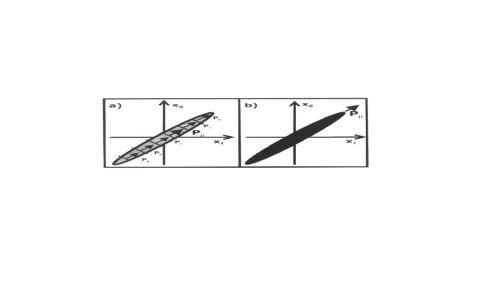
Figure 6: Kinetic and potential excitations - a new image of particle wave duality. (a) The running plane waves carrying out the four-momentum $P_{\mu}$ and included in space-time localized region (being “spread out” on light-cone skeleton structure $\Lambda_{0},\Lambda_{1}$) are called the kinetic excitations. On the other hand the same four-momentum $P_{\mu}$ can be carried out by standing waves embraced by the same space-time localized region (b). This kind of standing waves is called the potential excitations. The potential excitations then represents compact quantum object running through the space.

There are two important remarks that help to understand better the case of kinetic excitations. The first is that action of Lorentz boost considered as the transformation of Minkowski frame is to be regraded as the passive transformation. In other words, the Lorentz (or Poincaré) symmetry group appears the symmetry of quantum states themselves. But this, in turn, means that time and length measures of all inertial frame are always the same. It was noticed [5] that relativistic description requires a clear distinction between the vital and frozen time meanings. To recollect, it was explained that vital time is the measure of pace of observed changes and does not undergo relativistic transformation rules. In contrary to this the frozen time, which gives us energy measure in sense of inverse time units, does. Above analysis then suggests that frozen time meaning enters also description of quantum object extensions.

The second thing is that probability distributions provided by normalizable solutions of covariant oscillator equation are Lorentz invariants [7],[8]. In particular the space-time area of maximum probability density for kinetic excitation (44), due to light-cone skeleton deformation (8), is proportional to $\lambda_{1}\times\lambda_{2}$ $\sim 1/m_{0}^{2}.$ These features, however, become visible only in the light-cone coordinate frame. It was Kim who suggested to use the light-cone coordinate system as a natural language for Lorentz covariant phase-space representation of quantum mechanics [7]. It seems, however, that even more likely is a scenario at which descriptions based simultaneously on the Minkowski, as well as, light-cone frame, play the roles that are of equal importance and complementary. The issue, one may say, resembles almost a watching of $3d$ object at the real space. To get its complete image, in general, one needs to look at it more than just only one of its side. Similarly, a picture of extended quantum object emerging from the solutions of relativistic oscillator equation needs the light-cone coordinate system to become visible. On the other hand, the other quantum object properties such as its four-momentum or the time of life need the Minkowski frame (observation) to be established.

4.2 Potential excitations

The potential excitations were identified with the vibrations of internal particle structure, thereby describing them standing waves (33) might be called the potential states too. Similarly like in the case of kinetic excitations, the issue of potential states considered within the context of preferred frame description gives rise to a question about their physical meaning. Especially, what happens if the potential state is boosted and what is the influence on its physical meaning then? In this subsection we focus mainly on the first part of this question.

Generic example of the boost of the ground state (43) showed us that along with particle energy increase the space-time area embracing localized probability distribution, by simultaneous elongation and shrinking along the two orthogonal light-cone directions, undergoes the deformations too. The use photonic frame then enables potential states to become useful probabilistic toll against the background of relativistic preferred frame description. The important question is, however, whether the boost action affects the initial character of the excitations mode. In particular, whether it provides an admixture of “something else” that goes beyond the pure potential excitations. Fortunately the analysis of Kim and Noz in clear-cut way has resolved this problem.

Kim and Noz have shown that wave functions (31) constitute a linear infinite-dimensional unitary representation of the Lorentz group. As a result, one finds that potential state $\psi_{\lambda^{\prime}}(x),$ if boosted along $x_{1}$ direction, turns into the boosted one $\psi_{\lambda^{\prime},\eta}(x),$ which, in turn, can be made up of unboosted potential states again, namely

$$\psi_{\lambda^{\prime},\eta}(x) =\frac{1}{\pi}\left(\frac{1}{2}\right)^{\frac{l+m+n}{2}}\left(\frac{1}{l!m!n!}\right)^{\frac{1}{2}}H_{m}(x_{2})H_{n}(x_{3})$$ (45)

$$\times\left(\frac{1}{2}\left(\eta+\frac{1}{\eta}\right)\right)^{-(1+l)}exp\left(-\frac{1}{2}\left(x_{0}^{2}+x_{1}^{2}\right)\right)$$

$$\times\left(\underset{k=0}{\overset{\infty}{\sum}}\left(\frac{1}{4}\right)^{k}\left(\frac{\eta-\frac{1}{\eta}}{\eta+\frac{1}{\eta}}\right)^{k}H_{k}(x_{0})H_{l+k}(x_{1})\right),$$

So, the boost transformation performed on any potential state does not change its potential character at all. One needs to emphasize, however, that time-like excitations that do not appear at the level of effectively observed on-mass-shell, become inevitable components of internal (hidden-like) particle structure. It is worthwhile to notice also that notion of “particle rest frame” (in contrary to “observer rest frame”) turns out to be very tantalizing indeed.

The remaining aspect of the physical meaning of potential state boost is to be discussed next.

5 A new particle-wave duality picture emerging form relativistic oscillator model

The idea of particle-wave duality undoubtedly is one of the most crucial physical ideas that moulds our physical intuitions. The postulate of de Broglie

$$p=\frac{h}{\lambda},$$ (46)

which combines particle momentum $p$ with the wavelength $\lambda,$ and the postulate of Planck

$$E=\frac{h}{T},$$ (47)

which relates particle energy $E$ to the wave period $T$, set up the quantum-mechanical basis for this idea. The Schrödinger equation that put the postulates of Planck and de Broglie in “true” wave description reality, gave us a particle-wave duality picture, which, at the highest simplicity, is the following: the free particles are point-like whereas their wave-like nature is (successfully) represented by running (plane) waves or plane-wave packets. The key point is, however, that relativistic quantum mechanics cannot not improve this picture essentially, unless the predictions resulting from the solutions of covariant harmonic oscillator equation become appreciated. The aim of this section is to provide a new picture of particle-wave duality emerging just form the relativistic oscillator equation. Although this new picture goes much beyond the framework of Schrödinger approach, the old Schrödinger painting seems to be encompassed by the new one rather than challenged.

5.1 Oscillatory motion of extended quantum object

The explicit form of wave function (44) written at the Minkowski frame, due to (45), is

$$\phi_{0,\eta}(X,x)=e^{\pm\frac{i}{\hbar}\left(P_{\mu}X^{\mu}\right)}\cdot\left(\frac{1}{\pi}e^{-\frac{1}{2}\left(x_{0}^{2}+x_{0}^{2}+x_{2}^{2}+x_{3}^{2}\right)}\Psi_{\eta}(x_{0},x_{1})\right),$$ (48)

where

$$\Psi_{\eta}(x_{0},x_{1})=\left(\frac{1}{2}\left(\eta+\frac{1}{\eta}\right)\right)^{-1}\left(\underset{k=0}{\overset{\infty}{\sum}}\left(\frac{1}{4}\right)^{k}\left(\frac{\eta-\frac{1}{\eta}}{\eta+\frac{1}{\eta}}\right)^{k}H_{k}(x_{0})H_{l+k}(x_{1})\right).$$ (49)

Wave function (48) describes then extended quantum object which dynamical features and space-time extensions are linked through the light-cone skeleton structure.

The two separate factors that constitute wave function (48) describe respectively kinetic and potential excitations.  The “oscillatory logic” may suggest, however, that both kinds of excitations should be arranged in “oscillatory order”, i.e. kinetic (potential) excitation should follow the potential (kinematical) one and so on. Since $P_{\mu}P^{\mu}=m_{0}^{2}c^{2},$ the kinetic excitations provide us a picture of running plane waves carrying out the four-momentum $P_{\mu}$ , or alternatively, the image of point-particle endowed with the same four-momentum $P_{\mu}$. One needs to keep in mind, however, that the area of plane waves propagation is limited to the space-time region embraced basically by mentioned light-cone skeleton’s cover. On the other hand, the same light-cone skeleton provides us the space-time extensions of the potential state. But this in turn mens that the second factor of wave function (48) describes the particle in the form of extended material object moving through the space, as shown on Fig.6b. The wave function (48) provides then a new picture of particle-wave duality, as well as, a new description of particle motion. According to this the particle movement cannot be considered smooth but, as depicted on Fig.5, must take a form of oscillatory-like-motion.

5.2 The issue of uncertainty

The outlined above peculiar kind of motion inevitable must be accompanied by related energy and momentum fluctuations. To estimate the range of these fluctuations one finds the light-cone skeleton structure to become very useful again. It seems advisable, however, to recollect first the original concept of Heisenberg uncertainties referred to quantum measurement process.

Alongside the postulates of Planck (47) and de Broglie (46) there are also Heisenberg uncertainty principles

$$\Delta x\Delta p\simeq h,$$ (50)

and

$$\Delta\mathcal{E}\Delta\tau\simeq h,$$ (51)

that constitute the basis of Schrödinger quantum mechanics. It is widely believed that formula (50) describes relationship between the uncertainties of particle momentum $\Delta p$ and position $\Delta x$ in a measurement where both quantities are to be established at the same physical process. Similarly, if the subject of measurement is the particle energy, then related to this uncertainties of energy $\Delta\mathcal{E}$  and time $\Delta\tau$ (needed for such measurement) are assumed to be in relation (51). Seemingly both Heisenberg expressions have little to do with pure relativistic approach and it seems rather unlikely to incorporate them into rigid relativistic framework in a self-consistent way. Nevertheless, it turns out to be feasible. There are however two essential obstacles that need to be pointed out first.

The first remark concerns the underlying algebraic basis of  both uncertainty relations. Since the position and momentum are the $q-numbers$, i.e. position and momentum have operator representatives $\widehat{x}$ and $\widehat{p}$ for which it holds

$$\left[\widehat{x},\widehat{p}\right]=i\hbar,$$ (52)

relation (52) is a $q-number$ uncertainty relation. In contrary to this, as noticed by Dirac [9], the (vital) time is (only) a $c-number$, which mens that there is no Hilbert space associated to the time variable [10]. As a result it must occur

$$\left[t,\widehat{H}\right]=0,$$ (53)

where $\widehat{H}$ is energy operator or a Hamiltonian. Relation (53) then is a $c-number$ uncertainty relation. So, the emerging problem is that Heisenberg relations brought directly on the relativistic ground forces the Lorentz covariant description to deal with a mixture of $q-numbers$ and $c-numbers,$ which, as also noticed by Dirac [9], cannot be consistent with special relativity.

The problem might become much simpler, however, if relations (50) and (51) are to be considered not in terms of $q-$ and $c-numbers$ but in terms of wave packet average width-spreads. Let us then consider relation (50) and assume that it just relates the widths of wave packet spatial distribution $\Delta x$ and longitudinal momentum distribution $\Delta p$. However, if $\Delta x$ and $\Delta p$ are the quantities of Minkowski frame (as it is commonly thought), then the boost transformation turns the relation (50) into another one

$$\Delta x\Delta p\simeq h\cdot sinh2\xi,$$

which, of course, violates Heisenberg principle original form, thereby its universal character originally assumed [11],[12].

To overcome both mentioned difficulties Kim and Noz [4] showed up that proper formulation of uncertainty principles provide canonically conjugated Fourier components of wave function (43) i.e. the wave function described in the photonic frame. Indeed, under such circumstances relations (50) and (51) become the light-cone frame relations. As a result they become Lorentz-boost form invariants, thereby become also the integral part of the relativistic approach. The example of quantum object spread out on light-cone skeleton structure illustrates this idea too.

The light-cone skeletons shown on Figs.4a and 4b, are the skeletons of the same quantum object but considered respectively in position and momentum space. So that they are, of course, the mutually conjugated structures. In order to emphasize that relations (50) and (51) should be regarded as the light-cone ones let us apply a symbolic substitution

$$\Delta x\rightarrow\Delta\chi_{0},\text{ \ }\Delta p\rightarrow\Delta\pi_{1},$$ (54)

and similarly

$$c\Delta\tau\rightarrow\Delta\chi_{0},\text{ \ }\frac{\Delta\mathcal{E}}{c}\rightarrow\Delta\pi_{0}.$$ (55)

As a result one finds that relations (50) and (51), considered as the photonic frame uncertainty relations, become automatically fulfilled if uncertainty values (54) and (55) become identified with the light-cone skeleton extensions, i.e. when

$$\Delta\chi_{0}=\lambda_{0},\text{ }\Delta\chi_{1}=\lambda_{1},\text{ }\Delta\pi_{0}=\frac{h}{\lambda_{0}}\text{\ \ and }\Delta\pi_{1}=\frac{h}{\lambda_{1}}.$$ (56)

In order to return to the issue of oscillatory motion let us also answer the question how the light-cone uncertainty relations

$$\Delta\chi_{0}\Delta\pi_{0}\simeq h\text{ \ \ and \ \ }\Delta\chi_{1}\Delta\pi_{1}\simeq h,$$ (57)

appear to the observer rest frame. Let us then recollect that effectively observed particle dynamical and kinematical features, as it come from (2) and (9) are those of the Minkowski frame. So, the same must concern the energy and momentum fluctuations, which, then, must be determined by

$$\left(\begin{array}[c]{c}\frac{\Delta p_{0}}{2}\\ \frac{\Delta p_{1}}{2}\end{array}\right)=\left(\begin{array}[c]{cc}\frac{1}{\sqrt{2}}&\frac{-1}{\sqrt{2}}\\ \frac{1}{\sqrt{2}}&\frac{1}{\sqrt{2}}\end{array}\right)\left(\begin{array}[c]{c}\frac{\Delta\pi_{0}}{2}\\ \frac{-\Delta\pi_{1}}{2}\end{array}\right).$$ (58)

Thus, for the given values of light-cone momenta (56) one obtains that energy and momentum fluctuations are

$$\Delta E=E\text{ \ \ and\ \ \ }\Delta p=p.$$ (59)

So, for the particle of model shape one obtains that its energy and energy-fluctuations, as well as, momentum and momentum-fluctuations are the same. This just explains the occurrence of (perfect) transitions between kinetic and potential excitations, thereby oscillatory character of particle movement.

5.3 Heisenberg-Witten vs. Kim-Noz uncertainty relations

The broad issue of duality considered within the framework of string theory presumably is one of the most exploring ideas in contemporary theoretical physics. Even though the difficulty level even of quite simple string theory analysis exceeds much that of given in this paper, it seems justified to indicate some basic similarities that occur between the string theory and covariant harmonic oscillator approach. The first is that in the both cases one deals with space-time extended quantum objects instead of (field theory) point-particle image. Secondly, it turns out that the source of particle mass might be the string vibrations, so that the concept of mass no longer seem to be elementary. And finally, for the purpose of this paper, it is enough to indicate one more common feature of the both approaches. Supported by advanced calculations of Gross and Mende [13] and proposed in the context of duality in string theory, generalized Heisenberg uncertainty relation of Witten [14], is found to be exactly the one of Kim and Noz (57), however, being written at the Minkowski frame. It is worthwhile to take a closer look at this quite elementary issue.

Let us consider again Eq. (9) and focus on very time-like separation $\Delta x_{0}.$ Due to (6), which allows us to express $\Delta x_{0}$ by means of light-cone skeleton extensions $\lambda_{1}$ and $\lambda_{2},$ one obtains

$$\Delta x_{0}=\frac{1}{2}\lambda_{0}+\frac{1}{2}\lambda_{1}.$$ (60)

Expressed in a similar way the energy fluctuations (58) must take the form

$$\Delta E=\frac{1}{2}\frac{hc}{\lambda_{0}}+\frac{1}{2}\frac{hc}{\lambda_{1}}.$$ (61)

Eqs. (60) and (61) transparently reveal a dependence between quantum object space-time extensions and its dynamical features. According to (6) if particle stay at rest ($\eta=1$) both terms in both expressions (60) and (61) contribute the same. In such case the particle size is $\lambda_{C}$, which corresponds to $\Delta E=E=mc^{2}.$ However, along with energy increase ($\eta\nearrow$, cf. formulas (1) and (2)) only one term of each of the formulas (60) and (61) becomes dominant. Thus, even though the size of the whole quantum object grows ($\Delta x_{0}$ $\sim\lambda_{0}$), its energy fluctuations have still Heisenberg-like form, $\Delta E\Delta t\sim h$, where $\Delta t=\lambda_{1}/c.$ Furthermore, since the energy increase induces $\lambda_{1}$ decrease, dynamical consequences resulting from that make that point-particle picture is to become more accurate too. Nevertheless, as it comes from the discussion devoted to kinetic excitations, enlarged extensions of quantum object indicate also the space-time area where the “point-particle” can be found. In other words, the formulas (60) and (61), in simple quantum-mechanical manner, describe a new emerging picture of particle wave-duality. But this is exactly the same what does Witten formula predict. Indeed, by making use of property $\lambda_{0}\lambda_{1}=\lambda_{C}^{2}=(h/mc)^{2},$ one easily finds that expression (60) turns out to be (almost) the Witten formula

$$\Delta x_{0}=\frac{1}{2}\frac{h}{\Delta\pi_{0}}+\alpha_{m}^{\prime}\frac{1}{2}\frac{\Delta\pi_{0}}{h},$$ (62)

where $\alpha_{m}^{\prime}=(h/mc)^{2},$ and $\Delta\pi_{0}=\frac{h}{\lambda_{0}}$. Thus, to expose the (possibly crucial) role of minimal length scale (which is assumed to be the order of Planck length $l_{p}=\sqrt{hG/\left(2\pi c^{3}\right)}$ $\sim 1.6\cdot 10^{-35}m,$ and thus $\alpha_{m}^{\prime}\geqslant\alpha^{\prime}\equiv\left(l_{P}\right)^{2}$), as well as, to write down the Witten formula already in its exact form, due to (62), one may estimate minimal size of quantum object according to

$$\Delta x_{0}\geqslant\frac{1}{2}\frac{h}{\Delta\pi_{0}}+\alpha^{\prime}\frac{1}{2}\frac{\Delta\pi_{0}}{h}.$$ (63)

So, as one would expect, the Planck length $l_{P}$ is the Lorentz invariant indeed and, as it comes from above, there is no need to “double” relativity issue [15] to support that statement. Nevertheless, a particle cannot be seen as a material point but rather as an extended quantum object endowed with internal space-time structure.

6 Concluding remarks

It is widely believed that the origin of special relativity is purely the classical one. On the other hand, there is no doubt that there would be no Einstein theory if the Maxwell equations and observations of Michelson and Morley concerning the ether existence had become known first. The key point is, however, that “early observations” of electromagnetic interactions are thought to be the classical ones too. Even though that “classical electrodynamics” blows up the framework of Newtonian physics, the name “classical” does not seem to be used improperly. Given that electromagnetic field indeed is a true classical field (whatever it means) its quantum nature was already recognized by Planck at the problem of blackbody radiation, in 1901, i.e. before the special relativity came up. What’s more, the quantum nature of electromagnetic field was confirmed by Einstein himself  who discovered the photoelectric effect in 1905. Nevertheless the well-know Einstein’s stubbornness against comprehension of physical word in terms of quantum mechanics has been never overcame.

In 1935 Einstein, Podolsky and Rosen [16] (EPR) in an effort to rescue “locality” and “classical reality” introduced their famous Gedankenexperiment and proposed that quantum mechanics was incomplete. Let us then remind the Einstein locality principle [17]: “If $S_{1}$ and $S_{2}$ are the two systems that have interacted in the past but now are arbitrary distant, the real factual situation of system $S_{1}$ does not depend on what is done with system $S_{2},$ which is spatially separated from the former.” Then, the new class of models, called the Local Hidden-Variables (LHV) models, appeared to describe statistical features of quantum measurements as a result of underlying deterministic substructure. In 1964 Bell showed [18], however, that all LHV models that provide the results being in complete agreement with predictions of quantum mechanics do not obey the principle of locality, or, in other words, if substructures of LHV models appear to be truly local, their predictions must differ from those of quantum mechanics.

At early seventies, with the aid of Bell (inequalities) and available new experimental techniques, a new era of Gedankenexperiments begun and despite of EPR expectations the results it has provided have testified strongly against the classical ideology. The violation of Bell-inequalities were observed in a wide range of Gedankenexperiments based mainly on two-photons correlations measurements such as: polarization correlations [19], energy and time correlations (followed by experimental proposal of Franson [20]) [21] , or phase and momentum correlations [22].

Additionally, it is worthwhile to single out three more experimental observations that disclose unlocal properties of quantum states in very spectacular way, namely: the Franson and Potocki observation of “Single photon interference over large (45m) distances” [23], G. Weiss et al. [24] “Violation of Bell’s inequality under strict Einstein locality conditions”, and W. Tittel at al. [25] “Experimental demonstration of quantum correlations over more then 10 km.”

The era of Gedankenexperiments is basically finished and its heritage was taken over by Quantum Teleportation already originated over ten years ago [26]. Although above mentioned experimental results clearly indicate that tight keeping on Einstein’s locality idea contradicts the sober view, the issue of Lorentz symmetry, so far, has been never regarded in terms of the quantum approach seriously. Furthermore, even from the very theoretical point of view, one finds that Maxwell equations do occupy exactly the same position in quantum field theory approach as the equations of Dirac and Klein-Gordon do. Of course, these two material fields, until quantized, play the role of classical fields too. Nevertheless, devoid of the context of quantum mechanics they mean nothing. In the case of electromagnetic field and Lorentz symmetry the situation, presumably, is very similar.

And finally let us ask the fundamental question: is that because of Einstein’s time relativity idea looking so attractive, any alternative approach to “relativity issue” is simply out of the question? The honest answer is, perhaps, as hard as solutions of a few challenging physical problems. The author of the parer is aware of its simplicity, thereby far from the belief that presented now non-orthodox approach might be called satisfied. It seems, however, that even more important then any field theory analysis is to realize first how substantial and “positive flooding” consequences of departure form orthodox relativity perception might be. The main results of analysis already started in [5] and being continued now are summarized below in the form of concise comparison between some consequences resulting from orthodox and non-orthodox views.

$$\begin{array}[c]{cc}\text{ORTHODOX \ \ VIEW \ \ \ \ \ \ }&\text{NON-ORTHODOX VIEW\ }\end{array}\text{\ \ \ \ \ \ \ \ \ \ \ \ \ \ \ \ \ \ \ \ \ \ \ \ \ \ \ \ }$$

          General Meaning of Special Relativity

$$\begin{array}[c]{cc}\text{The Classical theory \ \ \ \ \ \ \ \ }&\text{The Tool of Quantum Mechanics\ \ \ \ \ }\end{array}$$

          The Special Relativity Source

$$\begin{array}[c]{cc}\text{Relativity of inetrial frames}&\text{Freedom of choice of comparison scale}\end{array}\text{ }$$

                                        maintained within the framework of preferred

frame quantum description

         The Emerging Particle Image

$$\begin{array}[c]{cc}\text{Point-like \ \ \ \ \ \ \ \ \ \ \ \ \ \ \ \ \ \ \ \ \ \ \ }&\text{Extended quantum object endowed with }\end{array}$$

                                        internal space-time structure

 Basic Relativity Predictions

$$\begin{array}[c]{cc}\text{Relativity of time and \ \ \ \ \ \ }&\text{Space-time deformations of quauntum }\end{array}\text{\ \ \ }$$

$$\begin{array}[c]{cc}\text{lenght maesure \ \ \ \ \ \ \ \ \ \ \ \ \ \ \ }&\text{object internal structure. }\end{array}$$

                                        Time and length measures remain intact

I would like to thank prof. W. Wójcik, prof. B. Kozarzewski and prof. A. Böhm for the financial support that allowed me to participate on the Second Feynman Festival conference held at the University of Maryland (August 2004, Collage Park, MD. U.S.A.)

References

- [1] R. P. Feynman, M Kislinger, and F. Ravndal, Phys. Rev. D 3, 2706 (1971).
- [2] Y. S. Kim and M. E. Noz, Phys. Rev. D 8, 3521 (1973); Y. S. Kim and M. E. Noz, Phys. Rev. D 15, 335 (1977).
- [3] Y. S. Kim, physics/0403027
- [4] Y. S. Kim and M. E. Noz, Theory and Applications of the Poincaré Group, (Reidel, Dordrecht, 1986).
- [5] P. Korbel, hep-th/0412267.
- [6] H. Yukawa, Phys. Rev. 91, 416 (1953).
- [7] Y. S. Kim and E. P. Wigner, Phys. Rev. A 36, 1293 (1987).
- [8] Y. S. Kim and E. P. Wigner, Phys. Rev. A 38, 1159 (1987); Y. S. Kim and M. E. Noz, Is the concept of quantum probability consistent with Lorentz covariance?, presented at the Second International Conference of Foundations of Probability in Physics (Vaxjo, Sweden, June 2002), quant-ph/0301155.
- [9] P. A. M. Dirac, Proc. Roy. Soc. (London) A114, 234 and 710 (1927).
- [10] C. H. Blanchard, Am. J. Phys. 50, 642 (1982).
- [11] D. Han, Y. S. Kim and M. E. Noz, Phys. Rev. A 35, 1682 (1987).
- [12] Y. S. Kim, Lorentz Covariance and Internal Space-time Symmetry of Relativistic Extended Particles, Contribution to the Nova Collection of papers on the Lorentz group (edited by Valeri Dvoeglazov), hep-th/9810538; Y. S. Kim Lorentz Boosts as Squeeze Transformations and the Parton Picture, presented at the Conference on Fundamental Interaction of Elementary Particles, An Annual Meeting of Particle and Nuclear Physics Division of the Russian Academy of Sciences (October 1995).
- [13] D. J. Gross and P.F. Mende, Nucl. Phys. B 303, 407 (1988); Phys. Lett. B197, 129 (1987).
- [14] E. Witten, Physics Today, April 1996, pp 24-30.
- [15] see G. Amelino-Camelia, Int. J. Mod. Phys. D 11, 35 (2002), gr-qc/0012051; J. Magueijo and L. Smolin, Phys. Rev. Lett. 88, 190403 (2002); G. Amelino-Camelia, Nature 418, 34 (2002).
- [16] A. Einstein, B. Podolsky and N. Rosen, Phys. Rev. 47, 777 (1935).
- [17] A. Einstein, in A. Einstein Philosopher Scientist, edited by P. Schilpp (Library of Living Philosophers, Evanston, I11., 1949).
- [18] J. S. Bell, Rev. Mod. Phys. 38, 447 (1966); Physics (Long Island City, NY) 1, 195 (1964).
- [19] Y. E. Shih and C. O. Alley, Phys. Rev. Lett. 61, 2921 (1987); Z.Y. Ou and L. Mandel, Phys. Rev. Lett. 61, 50 (1988); A. Aspect, J. Dalibard and G. Roger, Phys. Rev. Lett. 49, 1804 (1982), ibid., 47, 460 (1981); E. S. Fry and R. C. Thompson, Phys. Rev. Lett. 37, 465 (1976); S. J. Freedman and J. F. Clauser, Phys. Rev. Lett. 28 (1972).
- [20] J. D. Franson, Phys. Rev. Lett. 62, 2205 (1989).
- [21] P. R. Tapster, J. G. Rarity and P. C. M. Owens, Phys. Rev. Lett. 73, 1923 (1994); P. G. Kwiat, A. M. Steinberg and R. Y. Chiao, Phys. Rev. A 47, R2472 (1993); J. Brendel, E. Mohler and W. Martienssen, Europhys. Lett. 20, 575 (1992).
- [22] J. G. Rarity and P. R. Tapster, Phys. Rev. Lett 64, 2495 (1990).
- [23] J. D. Franson and K. A. Potocki, Phys. Rev. A 37, 2511 (1988).
- [24] G. Weihs et al., Phys. Rev. Lett. 81, 5039 (1998).
- [25] W. Tittel et al., Phys.Rev. A 57, 3229 (1998).
- [26] C. H. Bennett et al., Phys. Rev. Lett. 70, 1895 (1993).