Slow equivariant lump dynamics on the two sphere

Abstract

The low-energy, rotationally equivariant dynamics of $n$ ${\mathbb{C}}{{P}}^{1}$ lumps on $S^{2}$ is studied within the approximation of geodesic motion in the moduli space of static solutions ${\sf Rat}^{eq}_{n}$. The volume and curvature properties of ${\sf Rat}^{eq}_{n}$ are computed. By lifting the geodesic flow to the completion of an $n$-fold cover of ${\sf Rat}^{eq}_{n}$, a good understanding of nearly singular lump dynamics within this approximation is obtained.

1 Introduction

The ${\mathbb{C}}{{P}}^{1}$ model in $2+1$ dimensions is a field theory of Bogomol’nyi type, analogous in many respects to the Yang-Mills-Higgs and abelian Higgs models. It has a topological lower bound on energy, saturated by solutions of a first order self-duality equation. These solutions may be interpreted as topological solitons, called lumps, analogous to monopoles and vortices. They have various physical interpretations in theoretical high energy and condensed matter physics. If space is a Riemann surface $\Sigma$, then static lumps are holomorphic maps $\Sigma\rightarrow{\mathbb{C}}{{P}}^{1}$, the Cauchy-Riemann condition playing the role of the self-duality equation. The most fruitful approach to understanding the dynamics of $n$ moving lumps is, following Ward [19], to restrict the field dynamics to ${\sf M}_{n}$, the moduli space of degree $n$ static lumps. This is the geodesic approximation originally proposed by Manton for monopole dynamics [8]. It works well for vortex and monopole dynamics [3, 13, 17, 18], though it lacks a rigorous underpinning for lumps. As is well known, the reduced dynamics amounts to geodesic motion in $({\sf M}_{n},\gamma)$ where $\gamma$ is the $L^{2}$ metric, defined by the restriction to $T{\sf M}_{n}$ of the kinetic energy functional of the field theory. One important difference between lumps and monopoles or vortices is that $({\sf M}_{n},\gamma)$ is geodesically incomplete in the lump case [12], so the approximation predicts that lumps may collapse and form singularities in finite time.

In reducing to the geodesic approximation, we replace a nonlinear hyperbolic PDE (the field equation) by a finite system of nonlinear ODEs (the geodesic equation in ${\sf M}_{n}$).This is clearly a much simpler system in principle. It is still highly nontrivial to study its solutions, however, principally because it is usually impossible to obtain explicit formulae for the metric $\gamma$. The same is true for monopoles and vortices. For these systems, interesting progress has been made by imposing extra rotational symmetries on the geodesic problem, so as to reduce it to low-dimensional submanifolds of ${\sf M}_{n}$ [5]. In the present paper, we apply this technique to ${\mathbb{C}}{{P}}^{1}$ lumps moving on $\Sigma=S^{2}$, concentrating particularly on the behaviour of geodesics close to the singularities where lumps collapse. The ${\mathbb{C}}{{P}}^{1}$ model is more usually formulated on domain $\Sigma={\mathbb{C}}$. This is a bad choice from our viewpoint since the $L^{2}$ metric is undefined due to the presence of non-normalizable zero modes [19] (though one can study geodesic motion on the leaves of a foliation of ${\sf M}_{n}$ on which these bad zero modes are frozen [6]). This problem is absent when $\Sigma$ is a compact Riemann surface. The choice $\Sigma=S^{2}$ is particularly natural because then ${\sf M}_{n}$ (though not $\gamma$) coincides with the $\Sigma={\mathbb{C}}$ moduli space. Noting that ${\mathbb{C}}{{P}}^{1}\cong S^{2}$, if we choose stereographic coordinates $z,W$ on domain and codomain respectively, then a degree $n$ holomorphic map is simply

$$\phi:z\mapsto W(z)=\frac{a_{0}+a_{1}z+\cdots+a_{n}z^{n}}{b_{0}+b_{1}z+\cdots+b_{n}z^{n}}=\frac{p(z)}{q(z)}$$ (1.1)

where $p(z)$ and $q(z)$ have no common roots and at least one of $a_{n},b_{n}$ is nonzero. So ${\sf M}_{n}={\sf Rat}_{n}$, the space of degree $n$ rational maps [20]. There is a natural open inclusion ${\sf Rat}_{n}\hookrightarrow{\mathbb{C}}{{P}}^{2n+1}$, namely

$$W(z)\mapsto[a_{0},a_{1},\ldots,a_{n},b_{0},b_{1},\ldots,b_{n}]$$ (1.2)

whence ${\sf Rat}_{n}$ inherits the structure of a complex manifold. ${\sf Rat}_{n}$ is noncompact since it omits from ${\mathbb{C}}{{P}}^{2n+1}$ the complex codimension 1 variety on which $p$ and $q$ share roots. As $\phi$ approaches this missing set, one or more lumps collapse to infinitely thin spikes and disappear. It is known that $\gamma$ is Kähler with respect to this complex structure [15]. See [1, 15] for a comprehensive survey of the geometric properties of $({\sf Rat}_{1},\gamma)$.

In the next section we identify in each ${\sf Rat}_{n}$ a totally geodesic submanifold ${\sf Rat}^{eq}_{n}$, topologically cylindrical, consisting of those $n$-lumps invariant under a certain $SO(2)$ action. We compute the induced metric on ${\sf Rat}^{eq}_{n}$, also denoted $\gamma$, and the total volume of $({\sf Rat}^{eq}_{n},\gamma)$, which turns out to be finite and, somewhat surprisingly, independent of $n$. In section 3 we study the lift of $\gamma$ to the obvious $n$-fold cover of ${\sf Rat}^{eq}_{n}$, itself cylindrical. We show that the lifted metric extends to a metric on $S^{2}$ which is $C^{0}$ if $n\geq 2$, $C^{1}$ if $n\geq 3$ and $C^{2}$ if $n\geq 4$, and deduce the total Gauss curvature of ${\sf Rat}^{eq}_{n}$ for $n\geq 1$. There is strong numerical evidence that $({\sf Rat}^{eq}_{n},\gamma)$ may be isometrically embedded as a surface of revolution in ${\mathbb{R}}^{3}$, and we construct this surface numerically for small $n$. Finally, in section 4 we study the geodesic problem on $({\sf Rat}^{eq}_{n},\gamma)$ by lifting it to the $n$-fold cover. This allows us, in particular, to gain a good understanding of near singular geodesics.

2 The geometry of ${\sf Rat}^{eq}_{n}$

There is a natural isometric action of $G=SO(3)\times SO(3)$ on $({\sf Rat}_{n},\gamma)$ descending from the usual action of $SO(3)$ on $S^{2}\subset{\mathbb{R}}^{3}$, namely

$$({\cal O}_{1},{\cal O}_{2}):\phi\mapsto{\cal O}_{1}\circ\phi\circ{\cal O}_{2}^{-1}$$ (2.1)

where we have used ${\cal O}_{i}$ to denote both an element of $SO(3)$ and its action on $S^{2}$ [15]. Given any subgroup (indeed, subset) $K$ of $G$, the fixed point set ${\sf Rat}_{n}^{K}$ of $K$ in ${\sf Rat}_{n}$ is, if a submanifold, a totally geodesic submanifold of $({\sf Rat}_{n},\gamma)$: geodesics which start on and tangential to ${\sf Rat}_{n}^{K}$ remain on ${\sf Rat}_{n}^{K}$ for all subsequent time [11]. Consider the following subgroup $K\cong SO(2)$:

$$K=\{(R(n\alpha),R(\alpha)):\alpha\in{\mathbb{R}}\},\quad\mbox{where}\quad R(\alpha)=\left(\begin{array}[]{ccc}\cos\alpha&-\sin\alpha&0\\ \sin\alpha&\cos\alpha&0\\ 0&0&1\end{array}\right).$$ (2.2)

Let us denote its fixed point set ${\sf Rat}^{eq}_{n}$. For later convenience, we also define a $SO(2)$ subgroup of purely spatial rotations:

$$K_{0}=\{(0,R(\alpha)):\alpha\in{\mathbb{R}}\}.$$ (2.3)

In terms of stereographic coordinates, the action of $K$ is

$$W(z)\mapsto e^{in\alpha}W(e^{-i\alpha}z).$$ (2.4)

We may split ${\sf Rat}_{n}$ into $U_{0}$, the subset on which $b_{0}\neq 0$ and its complement. On $U_{0}$, we may uniquely write $W(z)$ in the form

$$W(z)=\frac{a_{0}+a_{1}z+\cdots+a_{n}z^{n}}{1+b_{1}z+\cdots+b_{n}z^{n}}.$$ (2.5)

If $W(z)\in U_{0}\cap{\sf Rat}^{eq}_{n}$ then for all $z$ and $\alpha$

$$\frac{a_{0}e^{in\alpha}+a_{1}e^{(n-1)i\alpha}z+\cdots+a_{n}z^{n}}{1+b_{1}ze^{-i\alpha}+\cdots+b_{n}e^{-in\alpha}z^{n}} = \frac{a_{0}+a_{1}z+\cdots+a_{n}z^{n}}{1+b_{1}z+\cdots+b_{n}z^{n}}$$ (2.6)

by (2.4), and hence

$$a_{0}=a_{1}=\cdots=a_{n-1}=b_{1}=b_{2}=\cdots=b_{n}=0,\quad a_{n}\neq 0.$$ (2.7)

Any rational map in the complement of $U_{0}$ may be uniquely written

$$W(z)=\frac{1+a_{1}z+\cdots+a_{n}z^{n}}{b_{1}z+\cdots+b_{n}z^{n}},$$ (2.8)

since $a_{0},b_{0}$ cannot both vanish, by the no common roots condition. Hence if $W(z)\in{\sf Rat}^{eq}_{n}$ and $W(z)\notin U_{0}$, then for all $z$ and $\alpha$

$$\frac{e^{in\alpha}+a_{1}e^{(n-1)i\alpha}z+\cdots+a_{n}z^{n}}{b_{1}ze^{-i\alpha}+\cdots+b_{n}e^{-in\alpha}z^{n}}=\frac{1+a_{1}z+\cdots+a_{n}z^{n}}{b_{1}z+\cdots+b_{n}z^{n}}$$ (2.9)

which has no solution. Hence ${\sf Rat}^{eq}_{n}\subset U_{0}$:

$${\sf Rat}^{eq}_{n}=\{az^{n}:a\in{{\mathbb{C}}^{\times}}\}.$$ (2.10)

Clearly ${\sf Rat}^{eq}_{n}$ is a noncompact complex submanifold of ${\sf Rat}_{n}$ of complex dimension 1, biholomorphic to $S^{2}\backslash\{0,\infty\}$.

Physically, ${\sf Rat}^{eq}_{n}$ should be thought of as the space of coincident $n$-lumps located at either the north or the south pole of the domain $S^{2}$. If $a=\chi e^{i\psi}$, then $\chi\in{\mathbb{R}}^{+}$ describes the shape of the $n$-lump, while $\psi$ is its internal phase. The case $n=1$ was described in [14], so let us assume $n\geq 2$. The energy density ${\cal E}=\frac{1}{2}|d\phi|^{2}$ is $K_{0}$ invariant, ${\cal E}(z)={\cal E}(e^{-i\alpha}z)$, hence independent of $\psi$, and is localized in a band centred on a circle of constant latitude, as illustrated in figure 1. Note that if $\chi\gg 1$ ($\chi\ll 1$), the energy accumulates towards the South pole (North pole), although ${\cal E}$ vanishes identically at the poles themselves. One should bear in mind that geodesics in ${\sf Rat}^{eq}_{n}$ correspond to $n$-lump motions in which the shape varies in this one-parameter family and the internal phase simultaneously varies. The coincident lump position occupies only the two polar values, though the band of maximum energy density does move up and down smoothly.

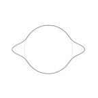
Figure 1: The energy density ${\cal E}$ of $W(z)=\chi z^{5}$ with $\chi=1$, $1/50$ and $1/50000$ respectively. Depicted are vertical cross sections through the graph of ${\cal E}$, plotted radially outwards as a non-negative function on $S^{2}$. The complete graphs are rotationally symmetric about the vertical axis.

Note that $K$ invariance is an admissible equivariance constraint for the full field equation also. If we let $z=re^{i\varphi}$, then the ${\mathbb{C}}{{P}}^{1}$ field equation is

$$\frac{4}{(1+r^{2})^{2}}\left[W_{tt}-\frac{2\bar{W}W_{t}^{2}}{1+|W|^{2}}\right]=W_{rr}+\frac{W_{r}}{r}+\frac{W_{\varphi\varphi}}{r^{2}}-\frac{2\bar{W}}{1+|W|^{2}}\left(W_{r}^{2}+\frac{W_{\varphi}^{2}}{r^{2}}\right)$$ (2.11)

which supports solutions within the $K$ invariant ansatz

$$W(r,\theta,t)=r^{n}a(r,t)e^{in\varphi}$$ (2.12)

for any $n\in{\mathbb{Z}}$. While the complex valued function $a(r,t)$ is $C^{1}$, nonvanishing and has limits at $r=0,\infty$ such solutions have degree $n$. We may regard geodesic flow in $({\sf Rat}^{eq}_{n},\gamma)$ as the geodesic approximation to this symmetry reduced field dynamics, or as a symmetry reduction of the geodesic approximation to the unreduced field dynamics.

The metric on ${\sf Rat}^{eq}_{n}$ is $K_{0}$ invariant and hermitian, so

$$\gamma=F(\chi)(d\chi^{2}+\chi^{2}d\psi^{2})$$ (2.13)

for some smooth positive function $F$. Let $\sigma:S^{2}\rightarrow S^{2}$ denote the isometry $z\mapsto z^{-1}$ (rotation by $\pi$ about the $x_{1}$ axis), and $\hat{\sigma}$ denote the corresponding isometry of ${\sf Rat}_{n}$, that is, $\phi\mapsto\sigma\circ\phi\circ\sigma^{-1}$. Since $\hat{\sigma}$ preserves ${\sf Rat}^{eq}_{n}$, in coordinates $\hat{\sigma}:(\chi,\psi)\mapsto(\chi^{-1},-\psi)$, it is an isometry of ${\sf Rat}^{eq}_{n}$, so from equation (2.13),

$$\hat{\sigma}^{*}\gamma=\chi^{-4}F(\chi^{-1})(d\chi^{2}+\chi^{2}d\psi^{2})=\gamma\quad\Rightarrow\quad F(\chi^{-1})\equiv\chi^{4}F(\chi).$$ (2.14)

It suffices, therefore, to understand the geometry of the “hemisphere” of ${\sf Rat}^{eq}_{n}$ where $0<\chi\leq 1$. To deduce $F(\chi)$, we must compute the squared $L^{2}$ norm of the zero mode $\partial/\partial\chi\in T_{(\chi,0)}{\sf Rat}^{eq}_{n}$, that is, twice the initial kinetic energy of the field $W(z,t)=(\chi+t)z^{n}$:

$$F(\chi)=\int_{\mathbb{C}}\frac{dzd\overline{z}}{(1+|z|^{2})^{2}}\frac{|\dot{W}(z,0)|^{2}}{(1+|W(z,0)|^{2})^{2}}=2\pi\int_{0}^{\infty}\frac{dr}{(1+r^{2})^{2}}\frac{r^{2n+1}}{(1+\chi^{2}r^{2n})^{2}}.$$ (2.15)

To be consistent with previous work, we have given both domain and codomain the metric $(1+|z|^{2})^{-1}dzd\overline{z}$, or equivalently, radius $\frac{1}{2}$. The $L^{2}$ metric for maps between spheres of radii $R_{1}$ and $R_{2}$ is easily deduced from this:

$$\gamma^{\prime}=16R_{1}^{2}R_{2}^{2}\gamma.$$ (2.16)

The even function $F:{\mathbb{R}}\rightarrow{\mathbb{R}}^{+}$ defined in (2.15) is smooth by, for example, repeated application of Lemma 2.2 from [15]. Since the integrand in (2.15) is rational, $F(\chi)$ can be computed explicitly, in principle, for any $n\in{\mathbb{Z}}^{+}$, though in practice the expressions become so complicated as to be useless as $n$ increases. The integral formula (2.15) turns out to be far more useful than the explicit expressions in any case. A striking illustration of this is

Proposition 1

${\sf Rat}^{eq}_{n}$ has volume $\pi^{2}$, independent of $n$.

Proof:

$${\rm Vol}({\sf Rat}^{eq}_{n}) = \int_{0}^{2\pi}d\psi\int_{0}^{\infty}d\chi\,\chi F(\chi)=4\pi^{2}\int_{0}^{\infty}d\chi\int_{0}^{\infty}\frac{dr}{(1+r^{2})^{2}}\frac{\chi r^{2n+1}}{(1+\chi^{2}r^{2n})^{2}}$$

$$= 4\pi^{2}\int_{0}^{\infty}\frac{dr\,r}{(1+r^{2})^{2}}\int_{0}^{\infty}d\chi\,r^{n}\,\frac{r^{n}\chi}{(1+(r^{n}\chi)^{2})^{2}}$$

$$= 4\pi^{2}\left[\int_{0}^{\infty}\frac{d\alpha\,\alpha}{(1+\alpha^{2})^{2}}\right]^{2}=\pi^{2},$$

where we have applied Tonelli’s Theorem [10].$\quad\Box$

Of more direct consequence for the geodesic flow on ${\sf Rat}^{eq}_{n}$ is an understanding of the singularity of $\gamma$ as $\chi\rightarrow 0$, hence, by the isometry $\hat{\sigma}$, also as $\chi\rightarrow\infty$. Such understanding is obtained by lifting $\gamma$ to the $n$-fold cover of ${\sf Rat}^{eq}_{n}$.

3 The lifted metric

There is a natural $n$-fold cover of ${\sf Rat}^{eq}_{n}\cong{{\mathbb{C}}^{\times}}$ by ${{\mathbb{C}}^{\times}}$ itself, namely $\pi:c\mapsto c^{n}$. In terms of polar coordinates $c=\rho e^{i\lambda}$, $\pi:(\rho,\lambda)\mapsto(\chi,\psi)=(\rho^{n},n\lambda)$. The lifted metric $\widetilde{\gamma}=\pi^{*}\gamma$ on ${{\mathbb{C}}^{\times}}$ is

$$\widetilde{\gamma}=\widetilde{F}(\rho)(d\rho^{2}+\rho^{2}d\lambda^{2})\quad\mbox{where}\quad\widetilde{F}(\rho)=n^{2}\rho^{2n-2}F(\rho^{n}).$$ (3.1)

In fact, rather than deduce an integral formula for $\widetilde{F}$ from that for $F$, it is easier to compute $\widetilde{F}(\rho)$ directly as the squared $L^{2}$ norm of the zero mode $\partial/\partial\rho$ in the family $W(z)=(\rho z)^{n}$,

$$\widetilde{F}(\rho)=\pi n^{2}\int_{0}^{\infty}\frac{ds}{(\rho^{2}+s)^{2}}\frac{s^{n}}{(1+s^{n})^{2}}$$ (3.2)

where we have used the substitution $s=(\rho|z|)^{2}$. Note that $\pi(1/c)=1/\pi(c)$, so $\hat{\sigma}:(\rho,\lambda)\mapsto(\rho^{-1},-\lambda)$ is an isometry of $\widetilde{\gamma}$, and hence

$$\widetilde{F}(\rho^{-1})\equiv\rho^{4}\widetilde{F}(\rho)$$ (3.3)

just as for $F(\chi)$. The integrand in (3.2) is globally bounded on $(0,\infty)$, independent of $\rho$, by $s^{n}(1+s^{n})^{-2}$, which is Lebesgue integrable if $n\geq 2$. Hence, by the Lebesgue dominated convergence theorem (LDCT [2])

$$\lim_{\rho\rightarrow 0}\widetilde{F}(\rho)=\pi n^{2}\int_{0}^{\infty}ds\lim_{\rho\rightarrow\infty}\frac{1}{(\rho^{2}+s)^{2}}\frac{s^{n}}{(1+s^{n})^{2}}=\pi n^{2}\int_{0}^{\infty}\frac{ds\,s^{n-2}}{(1+s^{n})^{2}}$$ (3.4)

which is finite and positive for $n\geq 2$. It follows that $\widetilde{\gamma}$ extends to a $C^{0}$ metric $\overline{\gamma}$ on $S^{2}={{\mathbb{C}}^{\times}}\cup\{0,\infty\}$, smooth away from $0$ and $\infty$. We suspect that $\overline{\gamma}$ is never (i.e. is for no $n\in{\mathbb{Z}}^{+}$) a smooth metric on $S^{2}$, but is $C^{k}$ provided $n\geq k+2$. For our purposes it will suffice to prove this for $k=1$ and $k=2$.

Proposition 2

The $C^{0}$ metric $\overline{\gamma}=\widetilde{F}(\rho)(d\rho^{2}+\rho^{2}d\lambda^{2})$ on $S^{2}$ is $C^{1}$ if $n\geq 3$ and $C^{2}$ if $n\geq 4$.

Proof: Since $\overline{\gamma}$ is smooth away from $\{0,\infty\}$ and $\hat{\sigma}$ is an isometry it suffices to check that $\overline{\gamma}$ is $C^{k}$, $k=1,2$, at $\rho=0$. So $\overline{\gamma}$ is $C^{1}$ if $\lim_{\rho\rightarrow 0}\widetilde{F}^{\prime}(\rho)=0$, and is $C^{2}$ if, in addition, $\lim_{\rho\rightarrow 0}\widetilde{F}^{\prime\prime}(\rho)-\widetilde{F}^{\prime}(\rho)/\rho=0$. Now

$$\widetilde{F}^{\prime}(\rho)=-4\pi n^{2}\rho\int_{0}^{\infty}\frac{ds}{(\rho^{2}+s)^{3}}\frac{s^{n}}{(1+s^{n})^{2}}=:-4\pi n^{2}\rho f(\rho).$$ (3.5)

The integrand of $f$ is dominated by $s^{n-3}(1+s^{n})^{-2}$ which is integrable if $n\geq 3$. Hence $\lim_{\rho\rightarrow 0}f(\rho)=\int_{0}^{\infty}ds\,s^{n-3}(1+s^{n})^{-2}<\infty$ by the LDCT, so $\lim_{\rho\rightarrow 0}\widetilde{F}^{\prime}(\rho)=0$ as required. Further,

$$\widetilde{F}^{\prime\prime}(\rho)-\frac{1}{\rho}\widetilde{F}^{\prime}(\rho)=-4\pi n^{2}\rho f^{\prime}(\rho)$$ (3.6)

and

$$\lim_{\rho\rightarrow 0}f^{\prime}(\rho)=\lim_{\rho\rightarrow 0}-6\rho\int_{0}^{\infty}\frac{ds}{(\rho^{2}+s)^{4}}\frac{s^{n}}{(1+s^{n})^{2}}=0$$ (3.7)

if $n\geq 4$ by appeal, once again, to the LDCT. $\Box$

This $C^{2}$ lift property has immediate consequences for the curvature properties of ${\sf Rat}^{eq}_{n}$. Let $\kappa$ and $\widetilde{\kappa}$ be the Gauss curvatures of $({\sf Rat}^{eq}_{n},\gamma)$ and $({{\mathbb{C}}^{\times}},\widetilde{\gamma})$. Since $\pi$ is by definition a local isometry, $\widetilde{\kappa}=\kappa\circ\pi$. If $n\geq 4$ then $\widetilde{\gamma}$ extends to a $C^{2}$ metric on $S^{2}$, compact, so $\widetilde{\kappa}$, and hence $\kappa$, must be bounded in this case. This should be contrasted with $({\sf Rat}^{eq}_{1},\gamma)$ whose Gauss curvature is unbounded above. We may also compute the total Gauss curvature of ${\sf Rat}^{eq}_{n}$ exactly:

Proposition 3

The total Gauss curvature of $({\sf Rat}^{eq}_{n},\gamma)$ is, for $n\geq 1$,

$$\int_{{\sf Rat}^{eq}_{n}}\kappa=\frac{4\pi}{n}.$$

Proof: Let $\Delta\subset{{\mathbb{C}}^{\times}}$ be the wedge $\Delta=\{\rho e^{i\lambda}\,:\,\rho\in{\mathbb{R}}^{+},\,0\leq\lambda<\frac{2\pi}{n}\}.$ Note that the local isometry $\pi:{{\mathbb{C}}^{\times}}\rightarrow{\sf Rat}^{eq}_{n}$ maps $\Delta$ bijectively onto ${\sf Rat}^{eq}_{n}$. Hence

$$\int_{{\sf Rat}^{eq}_{n}}\kappa=\int_{\Delta}\widetilde{\kappa}=\frac{1}{n}\int_{{\mathbb{C}}^{\times}}\widetilde{\kappa}$$ (3.8)

by $SO(2)$ invariance of $\widetilde{\gamma}$. If $n\geq 4$, the total Gauss curvature of $(S^{2},\overline{\gamma})$ is $4\pi$ since $\overline{\gamma}$ is sufficiently regular to apply the Gauss-Bonnet theorem. The total Gauss curvature of $({{\mathbb{C}}^{\times}},\gamma)$ is also $4\pi$ since $S^{2}\backslash{{\mathbb{C}}^{\times}}$ has measure $0$, and the result follows. To cover the cases $n=1,2,3$, one must resort to direct computation. Since

$$\widetilde{\kappa}=-\frac{1}{\rho\widetilde{F}(\rho)}\frac{d\,\,}{d\rho}\left(\frac{\rho\widetilde{F}^{\prime}(\rho)}{2\widetilde{F}(\rho)}\right)$$ (3.9)

we have that

$$\int_{{\mathbb{C}}^{\times}}\widetilde{\kappa}=4\pi\int_{0}^{1}d\rho\,\rho\widetilde{F}(\rho)\,\widetilde{\kappa}(\rho)=-4\pi\left[\frac{\rho\widetilde{F}^{\prime}(\rho)}{2\widetilde{F}(\rho)}\right]_{0}^{1}$$ (3.10)

where we have used the isometry $\hat{\sigma}$ to reduce the $\rho$ integral to $(0,1]$. Differentiating the identity (3.3) at $\rho=1$ shows that $\widetilde{F}^{\prime}(1)=-2\widetilde{F}(1)$, whence the result follows provided

$$\lim_{\rho\rightarrow 0}\frac{\rho\widetilde{F}^{\prime}(\rho)}{2\widetilde{F}(\rho)}=0.$$ (3.11)

We have already noted that $\lim_{\rho\rightarrow 0}\widetilde{F}(\rho)$ exists and is nonzero for $n\geq 2$, so it remains to show that $\lim_{\rho\rightarrow 0}\rho\widetilde{F}^{\prime}(\rho)=0$. This follows from the proof of Proposition 2 for $n\geq 3$, and may be checked easily for $n=2$ by computing $\rho\widetilde{F}^{\prime}(\rho)$ explicitly (using, for example, Maple) and evaluating the limit by hand. The case $n=1$ again requires us to calculate $\rho\widetilde{F}^{\prime}(\rho)$ explicitly, but now also $\widetilde{F}(\rho)$, take the ratio and then take the limit (using, for example, Maple again). $\Box$

The qualitative behaviour of geodesic flow on a surface depends crucially on the sign of $\kappa$. In this connexion we make

Conjecture 4

For all $n\geq 1$ $({\sf Rat}^{eq}_{n},\gamma)$ has positive Gauss curvature, and may be isometrically embedded as a surface of revolution in ${\mathbb{R}}^{3}$.

There is strong numerical evidence for Conjecture 4. Assume that such an embedding ${\bf x}:{\sf Rat}^{eq}_{n}\rightarrow{\mathbb{R}}^{3}$ does exist

$${\bf x}(\chi,\psi)=(\alpha(\chi),\beta(\chi)\cos\psi,\beta(\chi)\sin\psi).$$ (3.12)

We may construct its generating curve by equating $\gamma$ with the induced metric on ${\bf x}({\sf Rat}^{eq}_{n})\subset{\mathbb{R}}^{3}$,

$$(\alpha^{\prime}(\chi)^{2}+\beta^{\prime}(\chi)^{2})d\chi^{2}+\beta(\chi)^{2}d\psi^{2}=F(\chi)(d\chi^{2}+\chi^{2}d\psi^{2}).$$ (3.13)

This fixes $\beta(\chi)=\chi\sqrt{F(\chi)}$. To construct $\alpha(\chi)$ we solve the ODE

$$\frac{d\alpha}{d\chi}=\sqrt{F(\chi)}\sqrt{1-\left(1+\frac{\chi F^{\prime}(\chi)}{2F(\chi)}\right)^{2}}$$ (3.14)

with initial data $\alpha(1)=0$. Clearly, the solution exists whilever

$$-1\leq 1+\frac{\chi F^{\prime}(\chi)}{2F(\chi)}\leq 1,$$ (3.15)

which we find numerically holds true for all $\chi$ for $n=1,2,\ldots,6$. Inequality (3.15) has a nice geometric interpretation: let $\xi(\chi)$ be the angle between the $x_{1}$ axis and the tangent to the generating curve at $(\alpha(\chi),\beta(\chi))$. Then $\sin\xi(\chi)$ is precisely the function bounded in (3.15), so the generating curve exists precisely where $-1\leq\sin\xi(\chi)\leq 1$.

We have solved (3.14) numerically for $n=2,\ldots,6$, the resulting generating curves being diplayed in figure 2. Note that each curve is concave

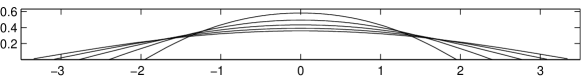
Figure 2: Generating curves for ${\sf Rat}^{eq}_{n}$, $n=2,\ldots 6$

down indicating that the surface it generates has positive Gauss curvature. If one changes parameters $\chi\mapsto\rho=\chi^{\frac{1}{n}}$, one finds

$$\sin\xi(\chi)=\frac{\rho\widetilde{F}^{\prime}(\rho)}{2n\widetilde{F}(\rho)}+\frac{1}{n}\,\,\stackrel{{\scriptstyle\chi\rightarrow 0}}{{\longrightarrow}}\,\,\frac{1}{n}\qquad(n\geq 1)$$ (3.16)

by the argument used to prove Proposition 3. Hence ${\sf Rat}^{eq}_{n}$, $n\geq 2$, has conical singularities of deficit angle

$$2\pi(1-\sin\xi(0))=2\pi(1-\frac{1}{n})$$ (3.17)

at $\chi=0$ and $\chi=\infty$. This gives an alternative interpretation of the proof of Proposition 3 in terms of the local Gauss-Bonnet theorem applied to the embedded surface of revolution [9]:

$$\int_{{\sf Rat}^{eq}_{n}}\kappa=2\pi(\sin\xi(0)-\sin\xi(\infty))=\frac{4\pi}{n}.$$ (3.18)

4 The geodesic flow

Consider the one parameter family of geodesics in $({\sf Rat}^{eq}_{n},\gamma)$ with initial data $a(0)=1$, $\dot{a}(0)=e^{i\alpha}$, $\alpha\in[0,\frac{\pi}{2}]$. This family contains all geodesics, up to isometries and time rescaling. A convenient way to construct such a geodesic is to lift the initial data to the covering space, $c(0)=1$, $\dot{c}(0)=e^{i\alpha/n}$, solve the geodesic equation in $({{\mathbb{C}}^{\times}},\widetilde{\gamma})$, then project, $a(t)=(\pi\circ c)(t)=c(t)^{n}$. Since $\pi$ is a local isometry, $a(t)$ is the required geodesic. The advantage of this is that, for $n\geq 4$, $\widetilde{\gamma}$ extends to a $C^{2}$ metric $\overline{\gamma}$ on $S^{2}$, which is just regular enough to ensure that the geodesic in $(S^{2},\overline{\gamma})$ exists for all time (by compactness) and depends continuously on the initial data. The point is that the geodesic equations involve only first derivatives of the metric coefficients, so if these coefficients are $C^{2}$, the flow function for the geodesic equation is $C^{1}$, hence locally Lipschitz, which is the minimal requirement for local existence, uniqueness and continuous dependence of solutions of an ODE system. So the lifting procedure allows one to construct reliably geodesics in $({\sf Rat}^{eq}_{n},\gamma)$ which approach arbitrarily close to the singularities at $\chi=0,\infty$, and even to define an unambiguous continuation of the singular geodesic ($\alpha=0$) (which travels along the curve $\psi=0$ from $\chi=0$ to $\chi=\infty$ in finite time by the estimate of [12]) beyond both the future and past singularities. In the lifted picture, the “singular” points $\rho=0$ and $\rho=\infty$ are not special, and the geodesic family varies continuously as it approaches and hits them.

Let the closest approach of $|c(t)|$ to $0$ for the $\alpha$ geodesic be $\delta>0$, very small. This is easily computed as a function of $\alpha$ using angular momentum and energy conservation. For $\delta$ sufficiently small, $c(t)$, being $C^{2}$, will be well approximated by a straight line on the $2\delta$ disk centred on $0$. Hence the projected geodesic $a(t)=c(t)^{n}$ will wind around the singularity $\chi=0$ $(n-1)/2$ times before exiting the $(2\delta)^{n}$ disk. To describe the corresponding field dynamics $W(z,t)$, we shall think of a configuration as a smooth distribution of classical spins over physical space $S^{2}$, as in the Heisenberg model of a ferromagnet. While $a(t)$ is in the $(2\delta)^{n}$ disk, the spins are all aligned almost exactly downwards except in a small neighbourhood of the north pole, where they vary rapidly (in space) in a charge $n$ bubble. Their energy is thus highly concentrated towards the north pole. As $c(t)$ traverses the $2\delta$ disk, the spins precess rapidly $(n-1)/2$ times about the north-south axis. The configuration then spreads out before reforming at the south pole and undergoing a similar rapid precession, and so on, indefinitely. In the limit $\delta\rightarrow 0$, one obtains an extended geodesic in which no spin precession occurs, but the configuration pinches to a point singularity at one pole, then spreads out to pinch at the opposite pole. There is a discontinuous phase flip (rotation of each spin by $\pm\pi$ about the north-south axis) associated with each pinch if $n$ is odd, but not if $n$ is even.

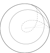
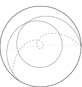
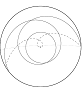
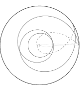
Figure 3: Geodesics in the disk $\chi\leq 1$ in ${\sf Rat}^{eq}_{n}$ when $n=2,3,4,5,6$

The above description is confirmed by numerical solution of the lifted geodesic problem. The equations were solved using a 4th order Runge Kutta method with variable time step. Energy and angular momentum were conserved to within $10^{-5}\,\%$. Figure 3 shows the projected geodesics in various cases. Although we can only prove global existence and continuous dependence of all lifted geodesics for $n\geq 4$, the lifting procedure seems to work well also for $n=2$ and $n=3$. This is not surprising given the presence of conical singularities in these cases, as explained in section 3. Of course, it is questionable whether geodesics which approach the singularities extremely closely really do accurately model the ${\mathbb{C}}{{P}}^{1}$ field dynamics. In fact, recent numerical [7] and analytic [4, 16] work gives some grounds for optimism in the equivariant $n\geq 2$ case.

Staying within the geodesic approximation, there are many interesting open questions about the $L^{2}$ geometry of ${\sf Rat}_{n}$ which require a good understanding of its boundary at infinity, so far lacking except in the case $n=1$. For example, is the volume and/or diameter finite? Is the spectrum of the Laplacian continuous or discrete (the answer having implications for quantum lump dynamics)? In this paper we have obtained a comprehensive understanding of the boundary at infinity of a (very) low dimensional totally geodesic submanifold of ${\sf Rat}_{n}$ which suggests that constructing natural $n$-fold covers of ${\sf Rat}_{n}$ may be a productive line of attack.

References

[1] J.M. Baptista,
“Some special Kähler metrics on and their holomorphic
quatization”
J. Geom. Phys.50 (2004) 1-27.
[2] Y. Choquet-Bruhat, C. DeWitt-Morette and M. Dillard-Bleick,
Analysis, Manifolds and Physics, Part I (North-Holland, Amsterdam,
1982) pp. 43-44.
[3] G.W. Gibbons and N.S. Manton, “Classical and quantum
dynamics of BPS monopoles” Nucl. Phys.B274 (1986)
183-224.
[4] M. Haskins and J.M. Speight,
“The geodesic approximation for lump dynamics and coercivity of the
Hessian for harmonic maps”
J. Math. Phys.44 (2003) 3470-3494.
[5] C. Houghton and P.M. Sutcliffe,
“ monopoles and Platonic symmetry”
J. Math. Phys.38 (1997) 5576-5589.
[6] R.A. Leese, “Low energy scattering of solitons in the
model” Nucl. Phys.B344 (1990) 33-72.
[7] J.M. Linhart and L.A. Sadun, “Fast and slow blowup in
the model and the -dimensional Yang-Mills
model”Nonlinearity15 (2002) 219-38.
[8] N.S. Manton, “A remark on the scattering of BPS
monopoles” Phys. Lett.110B (1982) 54-6.
[9] J. Oprea,
Differential Geometry and its Applications
(Prentice-Hall, London, UK, 1997) p205.
[10] H.A. Priestley, Introduction to Integration (Oxford
University Press, Oxford, UK, 1997), p193
[11] N.M. Romão,
“Dynamics of lumps on a cylinder”
preprint math-ph/0404008
[12] L. Sadun and J.M. Speight, “Geodesic incompleteness in
the model on a compact Riemann surface” Lett. Math. Phys.43 (1998) 329-34.
[14] J.M. Speight, “Low energy dynamics of a lump on
the sphere” J. Math. Phys.36 (1995) 796-813.
[15] J.M. Speight, “The geometry of spaces of harmonic
maps and ”
J. Geom. Phys.47 (2003) 343-368.
[16] M. Struwe,
“Equivariant wave maps in two space dimensions”
Comm. Pure Appl. Math.56 (2003)815-823.
[17] D. Stuart, “Dynamics of abelian Higgs vortices in the
near Bogomolny regime” Commun. Math. Phys.159 (1994) 51-91.
[18] D. Stuart, “The geodesic approximation for the
Yang-Mills-Higgs equations” Commun. Math. Phys.166 (1994)
149-90.
[19] R.S. Ward, “Slowly moving lumps in the model in
dimensions” Phys. Lett.158B (1985) 424-8.
[20] J.C. Wood,
“Harmonic maps and complex analysis” in Lectures of the
International Seminar on Complex Analysis and its
Applications, vol. III, Trieste, 1975, International Atomic Energy Agency,
Vienna, 1976, pp. 289-308.