The Hitchin functionals and the topological B-model at one loop

Abstract:

The quantization in quadratic order of the Hitchin functional, which defines by critical points a Calabi-Yau structure on a six-dimensional manifold, is performed. The conjectured relation between the topological $B$-model and the Hitchin functional is studied at one loop. It is found that the genus one free energy of the topological $B$-model disagrees with the one-loop free energy of the minimal Hitchin functional. However, the topological $B$-model does agree at one-loop order with the extended Hitchin functional, which also defines by critical points a generalized Calabi-Yau structure. The dependence of the one-loop result on a background metric is studied, and a gravitational anomaly is found for both the $B$-model and the extended Hitchin model. The anomaly reduces to a volume-dependent factor if one computes for only Ricci-flat Kahler metrics.

1 Introduction

In [1, 2, 3] it was suggested that the Hitchin functional $H(\rho)$ defined in [4] for real 3-forms on a 6-dimensional manifold $X$ is related to the topological $B$-model [5, 6, 7, 8] with the same target space $X$. Moreover in [1] a qualitative relation was proposed, which states that the partition function of the Hitchin model on $X$ is the Wigner transform of the partition functions of $B$ and $\bar{B}$ topological strings on $X$. See also [9, 10, 11]. That relation was tested in [1] at the classical level by evaluating the integral Wigner transform by the saddle point method.

The aim of the current work is to perform quantization of the Hitchin functional at the quadratic or one-loop order and to test the relation of it to the topological B-strings. It is known [8] that the one-loop contribution to the partition function of the $B$-model is given by the product of the holomorphic Ray-Singer $\bar{\partial}$-torsions $I^{RS}_{\bar{\partial},p}$ for the bundles of holomorphic $p$-forms $\Omega^{p,0}(X)$ on $X$:

$$F_{1}^{B}=\log\prod_{p=0}^{n}(I^{RS}_{\bar{\partial},p})^{(-1)^{p+1}p}.$$ (1)

The holomorphic Ray-Singer torsion for the $\bar{\partial}$-complex of the holomorphic vector bundle $\Omega^{p,0}$ is defined as the alternating product of the determinants of Laplacians acting on $(p,q)$ forms:

$$I^{RS}_{\bar{\partial},p}(\Omega^{p,0})=\left(\prod_{q=0}^{n}(\mathop{\rm det}\nolimits^{\prime}\Delta_{pq})^{(-1)^{q+1}q}\right)^{1/2}.$$ (2)

In terms of determinants, the formula for $F_{1}^{B}$ is [8]

$$F_{1}^{B}=\frac{1}{2}\log\prod_{p=0}^{n}\prod_{q=0}^{n}(\mathop{\rm det}\nolimits^{\prime}\Delta_{pq})^{(-1)^{p+q}pq}.$$ (3)

Alternatively, the one-loop factor in the $B$-model partition is

$$Z_{B,1-loop}=\exp(-F_{1}^{B})={\frac{I_{1}}{I_{0}^{3}}},$$ (4)

where we have used the fact that by Hodge duality, $I_{p}=I_{3-p}$.

In the present work, we show that after appropriate gauge fixing at the one-loop level, the partition function for the Hitchin functional $Z_{H,1-loop}$ also reduces to a product of holomorphic Ray-Singer torsions $I_{\bar{\partial},p}^{RS}$, but with different exponents from  (4).

We suggest resolving this discrepancy by considering instead of $H(\rho)$ the extended Hitchin functional $H_{E}(\phi)$ for polyforms $\phi$, which defines the generalized Calabi-Yau structure[12, 13] on $X$. (A polyform is simply a sum of differential forms of all odd or all even degrees.) The partition function of the extended Hitchin functional will be called $Z_{HE}$. The functional $H_{E}(\phi)$ was studied by Hitchin in his subsequent work [12, 13]. For CY manifolds $X$ with $b_{1}(X)=0$, the critical points and classical values of both functionals coincide. Hence the extended Hitchin functional $H_{E}(\phi)$ will also fit the check on classical level in [1] in the same way as $H(\rho)$. However the quantum fluctuating degrees of freedom are different for $H_{E}(\phi)$ and $H(\rho)$.

The precise statement about the relation between the full partition function of topological $B$-model and Hitchin functional still has to be clarified. In this paper, we will show that the one-loop contribution to the partition function of extended Hitchin theory is equal to the one-loop contribution to the partition function of the $B$-model

$$\boxed{F_{HE,1-loop}=F_{B,1-loop}}$$ (5)

The integral Wigner transform in [1], computed by the steepest descent method is equivalent at the classical level to the Legendre transform studied in [3]. The relation shall still hold for the first order correction. Thus the conjecture in [1] that $Z_{H}=Wigner[Z_{B}\otimes\bar{Z}_{B}]$ appears to contradict our result, since the extended Hitchin functional agrees with $Z_{B,1-loop}$ rather than its absolute value squared.

However, this apparent discrepancy has been explained to us by A. Neitzke and C. Vafa, as follows. Although formally it appears that the $B$-model partition function computed in genus $g$ should be holomorphic, this is in fact not so as there is a holomorphic anomaly [8]. In genus one, the role of the holomorphic anomaly is particularly simple; the genus one computation is symmetrical between the $B$-model and its complex conjugate, and apart from contributions of zero modes, one has $F^{B}_{1}=F^{B,hol}_{1}+c.c.$, where $F^{B,hol}_{1}$ is a holomorphic function of complex moduli. Hence $\exp(-F^{B}_{1})=|\exp(-F^{B,hol}_{1})|^{2}$. So our result (5) means that $Z_{HE,1-loop}=\exp(-F_{HE,1-loop})$ is equal to $|\exp(-F_{1}^{B,hol})|^{2}$. Further, $\exp(-F_{1}^{B,hol})$ must be understood as the one-loop factor in $Z_{B}$ in the conjecture of [1]. With this interpretation, our computation for the extended Hitchin functional agrees with the conjecture at one-loop order.

The appearance of the extended Hitchin functional for the generalized CY structures is appealing from the viewpoint of $\mathcal{N}=1$ string compactifications on 6-folds with fluxes [14, 15, 16, 17]. A study of the extended Hitchin functional for generalized complex structures, as opposed to ordinary ones, is also natural because the total moduli space of topological B-strings includes the space of complex structures, but has other directions as well, corresponding to the sheaf cohomology groups $H_{\bar{\partial}}^{q}(\mathop{\bigwedge}\nolimits^{p}(TX^{1,0}))$, where the case of $p=q=1$ yields the Beltrami differentials – deformations of the complex structure. See also [18, 19, 20, 21, 16, 22, 23, 24, 25, 26, 27, 28].

The paper has the following structure. In section 2, the Hitchin functionals are quantized at the quadratic order. Section 3 studies the dependence of the result on a background metric, and shows the presence of a gravitational anomaly. In general, the extended Hitchin and $B$-models are not invariant under a change of Kahler metric. The dependence on the Kahler metric does disappear, however, if we only use Ricci-flat Kahler metrics. Section 4 concludes the paper.

2 Quantization of the Hitchin functionals at the quadratic order

In [4, 12] Hitchin defines two functionals $H(\rho)$ and $H_{E}(\phi)$ that will be studied here.

The first functional $H(\rho)$ is defined for real 3-forms $\rho$ on a six-dimensional manifold $X$

$$H(\rho)=\int_{X}\phi(\rho).$$ (6)

Here $\phi(\rho)$ is a measure on $X$, defined as a nonlinear functional of a 3-form $\rho=\frac{1}{3!}\rho_{i_{1}i_{2}i_{3}}dx^{i_{1}}\wedge dx^{i_{2}}\wedge dx^{i_{3}}$ by

$$\phi(\rho)=\sqrt{-\lambda(\rho)}d^{6}x,$$ (7)

where

$$\lambda(\rho)=\frac{1}{6}\mathop{\rm Tr}K(\rho)^{2}$$ (8)

and the matrix $K^{b}_{a}(\rho)$ is given by

$$K^{b}_{a}(\rho)=\frac{1}{2!3!}\epsilon^{bi_{2}i_{3}i_{4}i_{5}i_{6}}\rho_{ai_{2}i_{3}}\rho_{i_{4}i_{5}i_{6}}.$$ (9)

Thus, $\phi(\rho)$ is the square root of a fourth order polynomial constructed from the components of the 3-form $\rho$. As Hitchin showed, each 3-form with $\lambda(\rho)<0$ defines an almost complex structure on $X$. This almost complex structure is integrable if $d\rho=0$ and $d\hat{\rho}=0$, where $\hat{\rho}$ is a certain 3-form constructed as a nonlinear function of $\rho$. In the space of closed 3-forms $\rho$ in a given cohomology class, the Euler-Lagrange equations are $d\hat{\rho}=0$. A critical point or classical solution hence defines an integrable complex structure $I$ on $X$ together with a holomorphic (3,0)-form $\Omega=\rho+i\hat{\rho}$. We will refer to an integrable complex structure with such a holomorphic $(3,0)$-form as a Calabi-Yau or CY structure.

To implement the restriction of $\rho$ to a particular cohomology class $[\rho_{0}]$, we write $\rho=\rho_{0}+db$, where $\rho_{0}$ is any three-form in the chosen cohomology class, and $b$ is a two-form that will be quantized. Of course, $b$ is subject to a gauge-invariance $b\to b+d\lambda$. It turns out that the second variation of the Hitchin functional $H(\rho)$ on the manifold $X$ is nondegenerate as a function of $b$ modulo the action of the group of diffeomorphisms $\mathop{\rm Diff}_{0}(X)$ plus gauge transformations. For $[\rho_{0}]$ in a certain open set in $H^{3}(X,\mathbb{R})$, the Hitchin functional has a unique extremum modulo gauge transformations and therefore produces a local mapping from $H^{3}(X,\mathbb{R})$ into the moduli space of CY structures on $X$.

The extended Hitchin functional [12] is designed to produce generalized complex structures [13] on $X$. To construct the extended functional, Hitchin replaces the 3-form $\rho$ by a polyform $\phi=\rho_{1}+\rho_{3}+\rho_{5}$, which is a sum of all odd forms. Any such polyform, if nondegenerate, defines a generalized almost complex structure on $X$ given by a “pure spinor”[29, 30, 31] $\phi+i\hat{\phi}$ with respect to $\mathop{\rm Spin}\nolimits(TX,TX^{*})$. If in addition $d\phi=0$ and $d\hat{\phi}=0$, then this generalized almost complex structure is integrable. If $b_{1}(X)=0$, then all generalized complex structures coincide with the usual ones. This will be the case under consideration in the present work. In this case, the critical points of the extended Hitchin model produce usual Calabi-Yau structure on $X$, but the fluctuating degrees of freedom are different, and therefore these two theories are different on a quantum level.

For the original Hitchin model, we write $\rho=\rho_{0}+db$, and obtain the partition function as a path integral over $b$,

$$Z_{H}([\rho_{0}])=\int Db\,e^{-H(\rho)}$$ (10)

where $b$ is a two form.

To study this functional at the one-loop level, one first needs to expand $H(\rho)$ around some critical point $\rho_{c}$, which describes a complex structure $I$ on $X$. This complex structure will be used to define the second variation of the functional.

Using the algebraic properties of $\phi(\rho)$, it is easy to compute the variation [4]. The first variation is given by

$$\delta\phi(\rho)=\delta\rho\wedge\hat{\rho}.$$ (11)

The second variation can be written in terms of the complex structure $J$ introduced by Hitchin [4] on the space of 3-forms $W=\mathop{\bigwedge}\nolimits^{3}(\mathbb{R}^{6})\otimes\mathbb{C}$. This complex structure $J$ commutes with the Hodge decomposition of $W$ with respect to $I$, and has the following eigenvalues

$$J=+i\quad\text{on}\quad W^{3,0},W^{2,1}$$ (12)

$$J=-i\quad\text{on}\quad W^{1,2},W^{0,3}.$$

The second variation of the Hitchin functional $H(\rho)$ is

$$H^{(2)}(\rho_{c},\delta\rho)=\delta^{2}_{\rho}H(\rho)=\int_{X}\delta\rho\wedge J\delta\rho.$$ (13)

Hence the one-loop quantum partition function for the Hitchin functional (6) is given by

$$Z_{H,1-loop}([\rho_{c}])=\int Db\,e^{-H^{(2)}(\rho_{c},db)},$$ (14)

where $\rho_{c}$ is a critical point of $H(\rho)$, which defines a complex structure on $X$.

In terms of the Hodge decomposition of the two-form $b$ with respect to the complex structure $I(\rho_{c})$ on $X$,

$$b=b_{20}+b_{11}+b_{02},$$ (15)

one gets

$$H^{(2)}(\rho_{c},db)=\int_{X}db\wedge Jdb=\int_{X}\partial b_{11}\wedge\bar{\partial}b_{11}.$$ (16)

The terms with $db_{20}$ and $db_{02}$ vanish. The form $db_{20}$ lies entirely in the $i$-eigenspace of $J$ and therefore $Jdb_{20}=idb_{20}$, but the wedge product of two exact forms gives zero after integration over $X$.

The reason that $b_{20}$ and $b_{02}$ do not appear in the action is that they can be removed by a diffeomorphism. Under a diffeomorphism generated by a vector field $V$, any 3-form $\rho$ transforms as $\delta\rho=(i_{V}d+di_{V})\rho$ (where $i_{V}$ is the action of contraction with $\rho$.) For $d\rho=0$, the transformation is just $\delta\rho=d(i_{V}\rho)$. As we have taken $\rho=\rho_{0}+db$, we can take the transformation of $b$ under an infinitesimal diffeomorphism to be simply $\delta b=i_{V}\rho$. For any $b$, there is a unique choice of $V$ that will set to zero $b_{20}$ and $b_{02}$; no determinant arises in this process, as there is no derivative in the transformation law $\delta b=i_{V}\rho$. The path integral will therefore be performed over $b_{11}$, with the remaining gauge invariance $\delta b_{11}=\bar{\partial}\lambda_{10}+\partial\lambda_{01}$.

To understand the quantization of the degenerate term $\int_{X}\partial b\wedge\bar{\partial}b$, it easier first to turn to the canonical example of the theory of an $n$-form field $f_{n}$ with action

$$S_{0}=-i\int_{X}f_{n}\wedge df_{n},$$ (17)

studied in [32, 33]. This theory leads to Ray-Singer torsion [34, 35, 36] for the de Rham complex, which appears as a resolution of the $d$ operator. See also [37, 38, 39, 40, 41] and [42, 33, 43, 44, 45]. Actually, we will only calculate the absolute value of the partition function of this theory. The partition function has a nontrivial phase, the $\eta$-invariant (see [46]), which arises because the action is indefinite. We will not discuss it here because it has no analog for the Hitchin theories that we will analyze later; hence, we will simply take the absolute values of all determinants.

It is instructive to first take the integral formally. Then, we turn to the BV formalism [47, 48, 49, 50, 45, 44], which is a powerful formalism for quantizing gauge theories such as this one with redundant or reducible gauge transformations. The derivation also shows that, if the cohomology groups $H^{k}(X)$ are nontrivial, the product of determinants that we get is best understood not as a number but as a measure on the space of zero modes. (Ideally, we would then get a number by integrating over the space of zero modes, but the meaning of this integral is a little unclear in the case of ghost zero modes.) A similar fact holds in the Hitchin theories, but we will not be so precise in that case.

The idea is just to directly integrate over the fields in the initial functional integral, and manipulate formally with the volume of zero modes. So, let us say that $n$ is odd and $f_{n}$ is bosonic, and consider the functional integral

$$Z_{fdf}=\frac{1}{\mathop{\rm Vol}\nolimits(G)}\int Df_{n}\,\,\exp(i\int f_{n}df_{n}).$$ (18)

Here ${\rm Vol}(G)$ is the volume of the gauge group. The operator $d$ acting on $f_{n}$ has an infinite-dimensional kernel, the space of closed forms $\Omega^{n}_{closed}$. Formally evaluating the integral, one gets

$$Z_{fdf}={\frac{1}{\mathop{\rm Vol}\nolimits(G)}}\left(\mathop{\rm det}\nolimits^{\prime}d_{n\to n+1}\right)^{-\frac{1}{2}}\mathop{\rm Vol}\nolimits(\Omega^{n}_{closed}),$$ (19)

where $\mathop{\rm det}\nolimits^{\prime}d_{n}$ is the determinant of the operator $d_{n}$ mapping $\Omega^{n}/\Omega^{n}_{closed}$ to its image in $\Omega^{n+1}$. The absolute value of this determinant is conveniently defined as $|\mathop{\rm det}\nolimits^{\prime}d_{n}|=\sqrt{\mathop{\rm det}\nolimits^{\prime}{d^{*}_{n+1}d_{n}}}$, where $\Delta^{\prime}_{n}=d^{*}_{n+1}d_{n}$ maps $\Omega^{n}/\Omega^{n}_{closed}$ to itself. The remaining factor is the volume of the kernel, which can be decomposed as

$$\mathop{\rm Vol}\nolimits(\Omega^{n}_{closed})=\mathop{\rm Vol}\nolimits(\Omega^{n}_{exact})\mathop{\rm Vol}\nolimits(H^{n}).$$ (20)

Now, using the map

$$\Omega^{n-1}\overset{d}{\longrightarrow}\Omega^{n}_{exact}$$ (21)

and recalling that the kernel of this map is $\Omega^{n-1}_{closed}$, one gets

$$\mathop{\rm Vol}\nolimits(\Omega^{n}_{exact})=\mathop{\rm Vol}\nolimits(\Omega^{n-1}/\Omega^{n-1}_{closed})\mathop{\rm det}\nolimits^{\prime}d_{n-1}=\frac{\mathop{\rm Vol}\nolimits(\Omega^{n-1})\mathop{\rm det}\nolimits^{\prime}d_{n-1}}{\mathop{\rm Vol}\nolimits(H^{n-1})\mathop{\rm Vol}\nolimits(\Omega^{n-1}_{exact}),}$$ (22)

where again we factored $\mathop{\rm Vol}\nolimits(\Omega^{n-1}_{closed})=\mathop{\rm Vol}\nolimits(H^{n-1})\mathop{\rm Vol}\nolimits(\Omega^{n-1}_{exact})$. Going recursively and expressing $\mathop{\rm Vol}\nolimits(\Omega^{n-1}_{exact})$ in terms of volumes of forms of lower rank one gets finally

$$Z_{fdf}={1\over{\rm Vol}(G)}\left(\mathop{\rm det}\nolimits^{\prime}d_{n\to n+1}\right)^{-\frac{1}{2}}\frac{\mathop{\rm det}\nolimits^{\prime}d_{n-1}\mathop{\rm det}\nolimits^{\prime}d_{n-3}\cdots}{\mathop{\rm det}\nolimits^{\prime}d_{n-2}\mathop{\rm det}\nolimits^{\prime}d_{n-4}\cdots}\,\cdot\,\frac{\mathop{\rm Vol}\nolimits H^{n}\mathop{\rm Vol}\nolimits H^{n-2}\cdots}{\mathop{\rm Vol}\nolimits H^{n-1}\mathop{\rm Vol}\nolimits H^{n-3}\cdots}\,\cdot\,\frac{\mathop{\rm Vol}\nolimits\Omega^{n-1}\mathop{\rm Vol}\nolimits\Omega^{n-3}\cdots}{\mathop{\rm Vol}\nolimits\Omega^{n-2}\mathop{\rm Vol}\nolimits\Omega^{n-4}\cdots}$$ (23)

Formally, to make sense of the theory, we must take the volume of the gauge group to be

$${\rm Vol{G}}=\frac{\mathop{\rm Vol}\nolimits\Omega^{n-1}\mathop{\rm Vol}\nolimits\Omega^{n-3}\cdots}{\mathop{\rm Vol}\nolimits\Omega^{n-2}\mathop{\rm Vol}\nolimits\Omega^{n-4}\cdots}.$$ (24)

(One can justify this intuitively by thinking of the gauge group as consisting of gauge transformations for fields, ghosts, ghosts for ghosts, and so on.) Any other definition of the volume that would lead to a sensible theory would differ from this one by the exponential of a local integral, which we could anyway absorb in the definition of the determinants. (In odd dimensions, there are no such local integrals in any case.)

Using some elementary facts about determinants that we explain momentarily, one obtains

$${\begin{aligned} Z\end{aligned}_{fdf}=I_{RS}^{1/2}\frac{\mathop{\rm Vol}\nolimits H^{n}\mathop{\rm Vol}\nolimits H^{n-2}\cdots}{\mathop{\rm Vol}\nolimits H^{n-1}\mathop{\rm Vol}\nolimits H^{n-3}\cdots}\\ }.$$ (25)

Here

$$I_{RS}=\prod_{p=0,\dots,2n}(\mathop{\rm det}\nolimits^{\prime}d_{p})^{(-1)^{p}}=\left(\prod_{p=0,\dots,2n+1}(\mathop{\rm det}\nolimits^{\prime}\,\Delta_{p})^{(-1)^{p+1}p}\right)^{\frac{1}{2}}$$ (26)

is the Ray-Singer torsion.

In general, to define a determinant of a linear operator that maps between two different vector spaces $H_{1}$ and $H_{2}$, one has to introduce a metric on them. Then, given a linear map $w:H_{1}\to H_{2}$, the absolute value of the determinant of $w$ is defined as

$$|\mathop{\rm det}\nolimits w|\equiv\sqrt{\mathop{\rm det}\nolimits(w^{*}w).}$$ (27)

In our problem, the Laplacian operator $\Delta_{p}$ acting on the space of $p$-forms $\Omega^{p}(X)$ is defined as

$$\Delta_{p}=dd^{*}+d^{*}d,$$ (28)

where $d^{*}$ is the Hodge conjugated differential $*d*$. This operator can be conveniently decomposed as follows:

$$\Delta_{p} =\,^{\prime}\Delta_{p}+\Delta_{p}^{\prime},$$ (29)

$${}^{\prime}\Delta_{p} =d_{p-1}d^{*}_{p},\quad\Delta^{\prime}_{p}=d^{*}_{p+1}d_{p}$$

The Hilbert space of $p$-forms can be Hodge decomposed as

$$\Omega^{p}=H^{p}\,\oplus\,^{\prime}\Omega^{p}\,\oplus\,\Omega^{\prime p},$$ (30)

where $H^{p}$ consists of harmonic forms, annihilated by both $d$ and $d^{*}$, ${}^{\prime}\Omega^{p}$ consists of forms annihilated by $d$ but orthogonal to harmonic forms, and $\Omega^{\prime}{}^{p}$ consists of forms annihilated by $d^{*}$ but orthogonal to harmonic forms. The nonzero eigenvalues of ${}^{\prime}\Delta_{p}$ span ${}^{\prime}\Omega^{p}$, and the nonzero eigenvalues of $\Delta_{p}^{\prime}$ span $\Omega^{\prime}{}^{p}$. $\Delta_{p}$ is zero on $H^{p}$, equals ${}^{\prime}\Delta_{p}$ on ${}^{\prime}\Omega^{p}$, and equals $\Delta_{p}^{\prime}$ on $\Omega^{\prime}{}^{p}$. Consequently,

$$\mathop{\rm det}\nolimits^{\prime}\Delta_{p}=\mathop{\rm det}\nolimits\,^{\prime}\Delta_{p}\,\mathop{\rm det}\nolimits\Delta^{\prime}_{p}.$$ (31)

where it is understood that $\mathop{\rm det}\nolimits^{\prime}\,\Delta_{p}$ is the product of the nonzero eigenvalues of $\Delta_{p}$ and that determinants of ${}^{\prime}\Delta_{p}$ and $\Delta^{\prime}_{p}$ are taken in ${}^{\prime}\Omega^{p}$ and $\Omega^{\prime}{}^{p}$. We also had

$$|\mathop{\rm det}\nolimits^{\prime}d_{p}|=\left(\mathop{\rm det}\nolimits\Delta^{\prime}_{p}\right)^{\frac{1}{2}},$$ (32)

and by Hodge symmetry $\mathop{\rm det}\nolimits^{\prime}\,\Delta_{p}=\mathop{\rm det}\nolimits^{\prime}\,\Delta_{2n+1-p}$. Finally, $\mathop{\rm det}\nolimits\,^{\prime}\Delta_{p}=\mathop{\rm det}\nolimits\Delta^{\prime}_{p-1}$. With these facts, we have $\prod_{p=0}^{2n+1}\mathop{\rm det}\nolimits^{\prime}\Delta_{p}^{(-1)^{p+1}p}=\prod_{p=0}^{2n}\mathop{\rm det}\nolimits{}(\Delta^{\prime}_{p})^{(-1)^{p}}$. Using these relations one gets (26).

Now we will repeat this discussion in the BV formalism, suppressing the role of the de Rham cohomology groups to keep things simple (for example, they may vanish if $f$ obeys twisted boundary conditions). In this approach, the gauge symmetries of the first stage for $f_{n}$ are the deformations by exact forms $df_{n-1}$

$$Qf_{n}=df_{n-1}$$ (33)

So the forms $f_{n-1}$ are the ghosts fields whose ghost number is $\#gh=1$, and of the opposite statistics to $f_{n}$. This gauge transformation is reducible, since the transformation (33) is trivial if $f_{n-1}=df_{n-2}$ for some $f_{n-2}$. Hence we introduce ghost number two fields $f_{n-2}$, sometimes called “ghosts for ghosts”:

$$Qf_{n-1}=df_{n-2}$$ (34)

The process is continued recursively, with

$$Qf_{k}=df_{k-1},\quad 0<k\leqslant n.$$ (35)

So the operator $Q$ of the BV complex is mapped to the differential $d$ acting on forms whose degree ranges from 0 to $n-1$.

So far we have introduced differential forms $f_{k}$, $0\leqslant k\leqslant n$, where $f_{n}$ are the original fields and the others are ghosts and ghosts for ghosts. The statistics of $f_{k}$ are $(-1)^{k+1}$. In the BV formalism, we need to introduce antifields, which are conjugate variables with opposite statistics. The conjugate variable to $f_{k}$ is simply a differential form $f_{2n+1-k}$, of statistics $(-1)^{k}=(-1)^{(2n+1-k)+1}$; the antibracket (odd Poisson bracket) is defined by the odd symplectic structure

$$\omega(f,g)=\int_{X}f\wedge g.$$ (36)

For all $0\leqslant k\leqslant 2n+1$, the ghost number of $f_{k}$ is $n-k$.

Having now the complete set of fields and antifields, and BRST transformations (35), we must next find the master action $S$ that coincides with the classical action for the original fields and such that $\{S,S\}=0$ and $\{S,f_{k}\}=Qf_{k}$ for all $k$. The reason that the BV formalism is so convenient for this particular problem is that the master action is very simple: the BV master action $S$ is

$$S=-i\sum_{k=0}^{n}\int f_{k}\wedge df_{2n-k}.$$ (37)

It has the same form as the classical action $S_{0}$, except that the fact that the constraint has degree $n$ is dropped. This fact has been used in analyzing Chern-Simons perturbation theory [40] and has a powerful analog for string field theory [51].

The resulting BV complex can be drawn as in fig. 1.

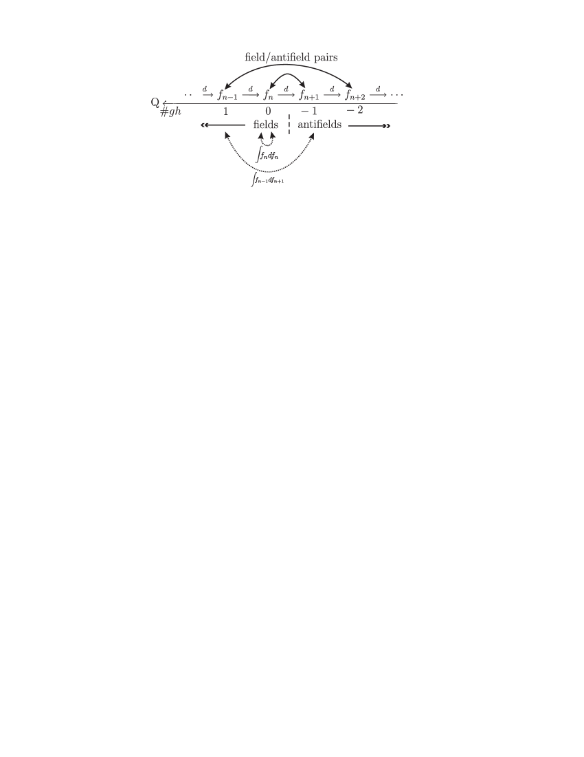
Figure 1: The BV complex for $\int_{X}df_{n}\wedge f_{n}$. Ghost number increases from right to left; the action of $Q$ increases the ghost number by 1.

The last step of the BV formalism is to choose a gauge fixing fermion $\Psi$, or, alternatively, to choose a Lagrangian submanifold in the function space of fields $f_{k}$. A convenient choice of Lagrangian submanifold $L$ is the space of $d^{*}$ closed forms

$$L:\quad d^{*}f_{k}=0.$$ (38)

By the Hodge decomposition (and our assumption of ignoring the de Rham cohomology), this condition is equivalent to restricting the fields $f_{k}$ to the orthocomplement of the space of gauge variations $Qf_{k}=df_{k-1}$. In all subsequent examples, we will similarly pick our Lagrangian submanifold to be the orthocomplement of the space of gauge variations.

After the restriction to the Lagrangian submanifold, the partition function of the theory with quadratic action (37) is equal to the alternating ratio of determinants of the differential operators $d_{k}$ mapping in the complex (39)

$$f_{0}\overset{d}{\longrightarrow}f_{1}\overset{d}{\longrightarrow}f_{2}\overset{d}{\longrightarrow}\dots\overset{d}{\longrightarrow}f_{n},$$ (39)

in the function space of differential forms $\Omega^{p}(X)/\Omega^{p}(X)_{closed}.$ Indeed, the gauge fixing condition $d^{*}_{k}f_{k}=0$ eliminates the kernels of the operators $d$ in (37), given that we assume the cohomology groups to be trivial. By a derivation that we have already seen, the alternating product of determinants of $d_{n}$ gives the following product:

$$Z_{fdf}=\left((\mathop{\rm det}\nolimits\Delta_{n}^{\prime})^{-1/4}\prod_{k=1}^{n}(\mathop{\rm det}\nolimits\Delta_{n+k}^{\prime})^{(-1)^{k}}\right)^{(-1)^{n+1}}=\left(\prod_{k=0}^{k=d-1}(\mathop{\rm det}\nolimits{\Delta^{\prime}_{k}})^{(-1)^{k}}\right)^{\frac{1}{4}}=I_{RS}^{\frac{1}{2}}$$ (40)

For the theory $S=\int_{X}f\wedge dg$, with a doubled set of variables, one has $Z_{fdg}=I_{RS}$.

The quadratic term of the Hitchin functional

Now consider the quadratic term of the Hitchin functional (16)

$$S=\int_{X}\partial b_{11}\wedge\bar{\partial}b_{11}.$$ (41)

To define the determinants of Laplacians that will appear in the evaluation of the partition function, one has to introduce a metric on $X$. The dependence on it will be analyzed later. We will use some Kahler metric $g$ compatible with the complex structure.

The Hodge diamond on  fig. 2,

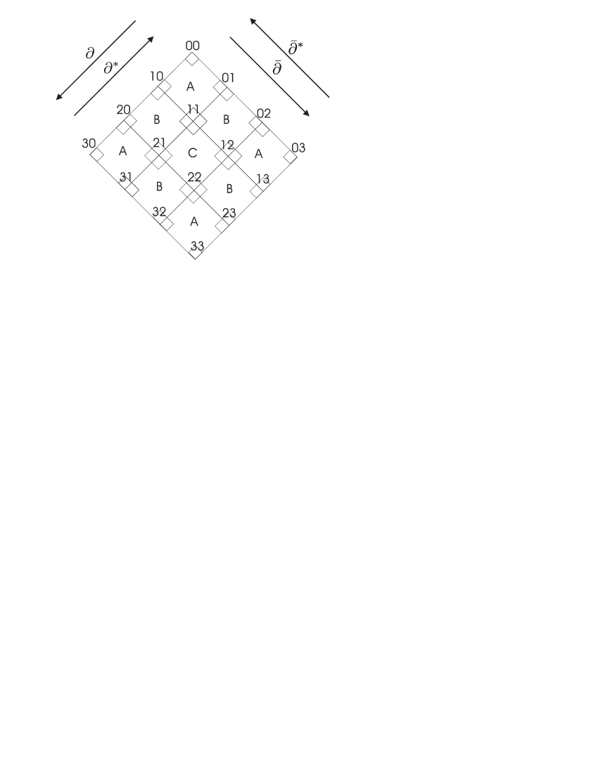
Figure 2: The Hodge diamond for a CY 3-fold. The type of forms is shown by label at vertices. The differential operators $\partial,\bar{\partial},\partial^{*},\bar{\partial}^{*}$ act along diagonal edges. The labels $A,B,C$ are associated with 9 square faces and are used to denote corresponding determinants of Laplacians. At each vertex, we have drawn some small squares, which will be used later to depict the Hodge decomposition. The meaning of the little squares is obtained later.

which is made of forms of different type $(p,q)$, can be sliced either into $\partial$ or $\bar{\partial}$ -complexes along the diagonal lines.

On a Kahler manifold, one has the relation [52]

$$\Delta_{\partial}=\Delta_{\bar{\partial}}=\frac{1}{2}\Delta_{d}$$ (42)

where

$$\Delta_{\bar{\partial}}=\bar{\partial}\bar{\partial}^{*}+\bar{\partial}^{*}\bar{\partial},\quad \Delta_{\partial}=\partial\partial^{*}+\partial^{*}\partial, \Delta_{d}=dd^{*}+d^{*}d$$ (43)

For a compact Kahler manifold, the cohomology groups $H^{p,q}$ are the same both for $\bar{\partial}$ and $\partial$ operator. They can be represented by the space of harmonic $(p,q)$ forms. Harmonic forms provide a unique representative in each $\bar{\partial}$-cohomology class. The same statement holds for $d$ and $\partial$ operators. Since on Kahler manifolds the $\partial$ and $\bar{\partial}$ Laplacians are equal

$$\Delta_{\partial}=\Delta_{\bar{\partial}},$$ (44)

the $\bar{\partial}$ and $\partial$ cohomology groups are represented by the same space of harmonic forms.

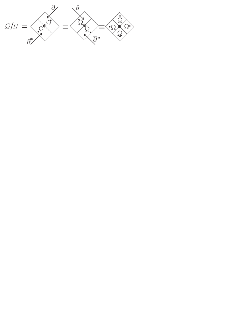
Figure 3: Three ways of decomposing $\Omega^{p,q}/H^{p,q}$. The idea of this figure and fig. 4 is to illustrate the decomposition of Hilbert spaces of forms into direct sums of subspaces. A Hilbert space, in this case $\Omega^{p,q}/H^{p,q}$, is represented as a square which is a union of rectangles or smaller squares that correspond to subspaces. In this example, for instance, the first decomposition is as the sum of images of $\partial$ and $\partial^{*}$. The others are as indicated. If $p$ or $q$ is 0 or 3, some pieces in these decompositions are missing, because forms of type $p,q$ cannot be reached by the action of certain operators.

The space $\Omega^{p,q}$ of forms of type $(p,q)$ can be Hodge decomposed either with respect to the operator $\bar{\partial}$ or the operator $\partial$. In the first case, one has

$$\Omega^{p,q}=H^{p,q}_{\bar{\partial}}\,\oplus\,\mathop{\rm Im}(\bar{\partial}(\Omega^{p,q-1}))\,\oplus\,\mathop{\rm Im}(\bar{\partial}^{*}(\Omega^{p,q+1})),$$ (45)

and in the second

$$\Omega^{p,q}=H^{p,q}_{\partial}\,\oplus\,\mathop{\rm Im}(\partial(\Omega^{p-1,q}))\,\oplus\,\mathop{\rm Im}(\partial^{*}(\Omega^{p+1,q})).$$ (46)

To shorten formulas, it is convenient to write

$$\Omega=H_{\bar{\partial}}\,\oplus\,^{\displaystyle\bullet}\Omega\,\oplus\,\Omega_{\displaystyle\bullet}$$ (47)

and

$$\Omega=H_{\partial}\,\oplus\,\Omega^{\displaystyle\bullet}\,\oplus\,_{\displaystyle\bullet}\Omega.$$ (48)

The $\bullet$-sign denotes the projection operator on the corresponding subspace in $\Omega^{p,q}$ in accordance with direction from which this subspace can be obtained by mapping by the $\bar{\partial}$ or $\partial$ operator, etc., as shown in fig. 3. In these formulas the indices ($p,q$) were suppressed to keep the notation visually simpler, but they should be kept in mind.

Since $\Delta_{\partial}=\Delta_{\bar{\partial}}$, one can further decompose $\Omega^{p,q}\equiv\Omega$. Namely, we define the projection to the “upper” and “lower” squares

$$\overset{\displaystyle\bullet}{\Omega}\,:=\,^{\displaystyle\bullet}\Omega\,\cap\,\Omega^{\displaystyle\bullet}$$ (49)

$$\underset{\displaystyle\bullet}{\Omega}\,:=\,_{\displaystyle\bullet}\Omega\,\cap\,\Omega_{\displaystyle\bullet}$$

and the “left” and “right” squares

$${\bullet}\Omega\,:=\,^{\displaystyle\bullet}\Omega\,\cap\,_{\displaystyle\bullet}\Omega$$ (50)

$$\Omega\bullet\,:=\,\Omega^{\displaystyle\bullet}\,\cap\,\Omega_{\displaystyle\bullet}$$

in fig. 3.

That is equivalent to

$${}^{\displaystyle\bullet}\Omega = \overset{\displaystyle\bullet}{\Omega} \oplus\,{\bullet}\Omega$$ (51)

$$\Omega^{\displaystyle\bullet} = \Omega\bullet \oplus\,\overset{\displaystyle\bullet}{\Omega}$$

$${}_{\displaystyle\bullet}\Omega = \underset{\displaystyle\bullet}{\Omega} \oplus\,{\bullet}\Omega$$

$$\Omega_{\displaystyle\bullet} = \underset{\displaystyle\bullet}{\Omega} \oplus\,\Omega\bullet$$

and altogether

$$\Omega=H\,\oplus\,\overset{\displaystyle\bullet}{\Omega}\,\,\oplus\,\Omega\bullet\,{}\oplus\,\,\underset{\displaystyle\bullet}{\Omega}\,\,\oplus\,\,{\bullet}\Omega.$$ (52)

For example, $\Omega$ with a dot above represents the subspace of $\Omega$ which is the image of $\partial\bar{\partial}$ acting from above, $\Omega$ with a dot to the right represents the image of $\partial\bar{\partial}^{*}$ acting from the right, etc. Pictorially, we represent this in fig. 3 by decomposing $\Omega$, or rather the orthocomplement to $H$ in $\Omega$, in terms of four little squares depicted on the right of the figure. (One could think of $H$ as living at the vertex at the center of the square.) In general, when we draw a Hodge diamond, each vertex is associated with such little squares, as shown in fig. 2.

The decomposition of $\Omega^{p,q}$ simplifies a little if $p$ or $q$ is equal to $0$ or 3, because then some of the summands in this decomposition vanish. This is clear in fig. 2, where a vertex on an edge or corner of the Hodge diamond has fewer little squares attached to it. Later we will also deal with reality conditions for forms. Without developing special notation, let us just summarize the idea in fig. 4.

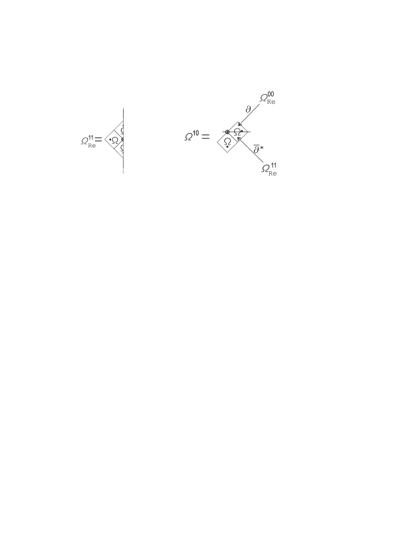
Figure 4: To depict the Hodge decomposition of a real form of type $(p,p)$, we introduce a vertical line and draw only one half of a square, symbolizing that the form is self-conjugate. The Hodge decomposition of a real form of type $(1,1)$ is sketched on the left; since ${\overset{\bullet}{\Omega}}{}^{11}$ and ${\underset{\displaystyle\bullet}{\Omega}}^{11}$ are real, they are depicted by little triangles rather than little squares, and as ${\Omega\bullet}{}^{11}$ is the complex conjugate of ${{\bullet}\Omega}^{11}$, only one of them is shown. More generally, we will usually only depict one of each complex conjugate pair of fields. Another subtlety arises in the Hodge decomposition when $\Omega^{pq}$ is complex but one of the spaces arising in its Hodge decomposition is real. On the right, we show this for $\Omega^{10}$. The little square depicting ${\Omega\bullet}^{10}$ is divided into upper and lower triangles representing $\partial$ of a real or imaginary $(0,0)$-form, respectively. Alternatively, they represent images of real forms of type $(0,0)$ and $(1,1)$, as shown.

Each projection operator from $\Omega$ to one of its “dotted” subspaces commutes with the Laplacian $\Delta_{\partial}=\Delta_{\bar{\partial}}$. And of course the Laplacian annihilates $H^{p,q}$. Therefore, the Laplacian on $\Omega^{p,q}$ can be decomposed into the sum defined by the projection operators $\bullet$

$$\Delta={\hat{0}}|_{H^{p,q}}\oplus\overset{\displaystyle\bullet}{\Delta}\,\oplus\,{\bullet}\Delta\,\oplus\,\Delta\!\bullet\,\oplus\,\underset{\displaystyle\bullet}{\Delta}.$$ (53)

Then the determinant of Laplacian restricted on $\Omega^{p,q}/H^{p,q}$ is a product

$$\mathop{\rm det}\nolimits^{\prime}\Delta=\mathop{\rm det}\nolimits(\overset{\displaystyle\bullet}{\Delta})\mathop{\rm det}\nolimits(\Delta\!\bullet)\mathop{\rm det}\nolimits(\underset{\displaystyle\bullet}{\Delta})\mathop{\rm det}\nolimits({\bullet}\Delta).$$ (54)

This formula holds for each $(p,q)$. Of course, the Laplacians with $\bullet$-sign do not contain zero eigenvalues, as all zero modes are contained in $H^{p,q}$.

To recapitulate all this, the Laplacians $\Delta_{p,q}$ are associated with the vertices in the Hodge diamond. On the other hand, the “halves” of Laplacians, defined by the “diagonal” $\bullet$-projections, ${}^{\displaystyle\bullet}\Omega$, $\Omega^{\displaystyle\bullet}$, etc., are naturally associated with diagonal edges between neighboring vertices. Finally, the “quarter” Laplacians, defined by the “left,” “right,” “up,” or “down” $\bullet$-projections $\overset{\displaystyle\bullet}{\Omega}$, $\Omega\bullet$, etc., are associated with the centers of squares or faces that connect four neighboring vertices in the Hodge diagram of fig. 2. Our notation is such that ${}^{\displaystyle\bullet}\Delta{}^{p,q}$ is the Laplacian associated with the edge that connects to vertex $(p,q)$ from the upper left, $\overset{\displaystyle\bullet}{\Delta}{}^{p,q}$ is the Laplacian associated with the face just above vertex $(p,q)$, etc.

The “quarter” or “face-centered” Laplacians are the elementary building blocks. The determinant of any other “vertex” or “edge” Laplacian can be constructed by multiplication. Moreover, on a CY manifold, the Laplacians satisfy more symmetry relations associated with symmetries of the Hodge diamond. They are induced by complex conjugation, Hodge $*$-conjugation, and multiplication by the holomorphic 3-form $\Omega$. For a 3-fold, these relations leave only 3 independent faces among the total of 9 in the Hodge diamond diagram: the 4 corner faces, the 4 edge-centered faces, and the central face. The “face” Laplacians will be denoted, respectively, as $\Delta_{A}$, $\Delta_{B}$, and $\Delta_{C}$, and their determinants as $A,B,$ and $C$. The 9 squares in fig. 2 have been labeled accordingly.

From the Hodge decompositions, we have

$$\mathop{\rm det}\nolimits^{\prime}\Delta_{00}=\mathop{\rm det}\nolimits^{\prime}\Delta_{33}=\mathop{\rm det}\nolimits^{\prime}\Delta_{30}=\mathop{\rm det}\nolimits^{\prime}\Delta_{03}=\mathop{\rm det}\nolimits\,\Delta_{A}=A,$$ (55)

$$\mathop{\rm det}\nolimits^{\prime}\Delta_{10}= \mathop{\rm det}\nolimits^{\prime}\Delta_{01}=\mathop{\rm det}\nolimits^{\prime}\Delta_{32}=\mathop{\rm det}\nolimits^{\prime}\Delta_{23}=$$ (56)

$$=\mathop{\rm det}\nolimits^{\prime}\Delta_{20}= \mathop{\rm det}\nolimits^{\prime}\Delta_{02}=\mathop{\rm det}\nolimits^{\prime}\Delta_{13}=\mathop{\rm det}\nolimits^{\prime}\Delta_{31}=\mathop{\rm det}\nolimits\Delta_{A}\mathop{\rm det}\nolimits\Delta_{B}=AB,$$

and finally

$$\mathop{\rm det}\nolimits^{\prime}\Delta_{11}=\mathop{\rm det}\nolimits^{\prime}\Delta_{21}=\mathop{\rm det}\nolimits^{\prime}\Delta_{12}=\mathop{\rm det}\nolimits^{\prime}\Delta_{22}=\mathop{\rm det}\nolimits\Delta_{A}(\mathop{\rm det}\nolimits\Delta_{B})^{2}\mathop{\rm det}\nolimits\Delta_{C}=AB^{2}C.$$ (57)

The Ray-Singer torsions $I_{p}$ with values in the holomorphic vector bundle $\Omega^{p,0}$ were defined in the introduction and can be written in terms of $A,B,C$:

$$I_{0}=I_{3}=(A^{2}B^{-1})^{1/2}=AB^{-1/2}$$ (58)

$$I_{1}=[(A^{2}B^{-1})(B^{2}C^{-1})]^{1/2}=AB^{1/2}C^{-1/2}.$$

The $B$-model partition function can be similarly written

$$Z_{B,1-loop}=I_{1}/I_{0}^{3}=(A^{-4}B^{4}C^{-1})^{1/2}.$$ (59)

Each face determinant appears to the plus or minus $1/2$ power, in a “chessboard” fashion, as shown later in fig. 7.

After recognizing the structure and decomposition of the relevant differential operators, one may proceed to the computation of of the partition function for the quadratic part of the Hitchin action,

$$S_{cl}=\int_{X}\partial b_{11}\wedge\bar{\partial}b_{11}.$$ (60)

The BV complex has the following structure. We start with physical fields $b_{11}$ and introduce ghosts $b_{10}$ and $b_{01}$, and fields $b_{00}$ of ghost number two (“ghosts for ghosts”). The reality conditions are obvious; $b_{pq}$ is complex conjugate to $b_{qp}$. The statistics of $b_{pq}$ for $p,q\leqslant 1$ are $(-1)^{p+q}$. Their BRST transformations are

$$Qb_{11}=\bar{\partial}b_{10}+\partial b_{01},$$ (61)

$$Qb_{10}=\partial b_{00},\quad Qb_{01}=\bar{\partial}b_{00}.$$

Now we introduce antifields, which are conjugate variables of opposite statistics. The conjugate of a form $b_{pq}$ is a form $b_{3-p,3-q}$, so the antifields are fields $b_{pq}$, $p,q\geqslant 2$, with statistics $(-1)^{p+q+1}$. The antibrackets are defined by the odd symplectic structure on the phase space of fields $\left\langle f,g\right\rangle=\int f\wedge g=(f,*g)$, where $(~{},~{})$ denotes the metric in the Hilbert space of $\Omega^{p,q}$ forms.

Now we must write down a master action $S$, which must reduce to $S_{cl}$ when the antifields are zero, generate the BRST transformations (61) when acting on the fields, and obey $\{S,S\}=0$. In the present problem, we can take $S=S_{cl}+S^{\prime}$, where

$$S^{\prime}=\sum_{i}\left\langle\Phi_{i}^{*},Q\Phi_{i}\right\rangle.$$ (62)

Here $\Phi_{i}$ ranges over all fields, namely the $b_{pq}$ of $p,q\leqslant 1$, and $\Phi_{i}^{*}$ are the corresponding antifields. To prove that $\{S,S\}=0$, we note that (i) $\{S_{cl},S_{cl}\}=0$ since $S_{cl}$ is independent of antifields; (ii) $\{S_{cl},S^{\prime}\}=0$, since when acting on fields, $S^{\prime}$ generates the transformation (61), under which $S_{cl}$ is invariant; (iii) $\{S^{\prime},S^{\prime}\}=2\sum_{i}\int\Phi_{i}^{*}Q^{2}\Phi_{i},$ which vanishes, since $Q^{2}=0$ on fields.

Having found the master action, we can also find the BRST transformations of antifields, as these are generated by $Q\Phi_{i}^{*}=\{S,\Phi_{i}^{*}\}$:

$$Qb_{22}=\partial\bar{\partial}b_{11}$$ (63)

$$Qb_{32}=\partial b_{22},~{}Qb_{23}=\bar{\partial}b_{22}.$$

Now we must choose a Lagrangian submanifold (again for simplicity neglecting the Hodge cohomology groups). As in our practice example, we define the Lagrangian submanifold to be the orthocomplement of the space of gauge variations. This can be defined using the projection operators that we have already constructed, and removes the kernels of all kinetic operators that appear in the master action.

In detail, the Lagrangian submanifold is defined by saying that for some forms $\alpha_{pq}$ of appropriate degrees, with $\alpha_{qp}=\bar{\alpha}_{pq}$, we have

$$b_{11} =\partial^{*}\bar{\partial}^{*}\alpha_{22}$$ (64)

$$b_{10} =\partial^{*}\alpha_{20}+i\partial\alpha_{00}$$

$$b_{01} =\bar{\partial}^{*}\alpha_{02}-i\bar{\partial}\alpha_{00}.$$

No condition is placed on $b_{00}$. Once we have selected these conditions on the fields, the corresponding conditions on the antifields are uniquely determined; the antifields must be constrained to obey

$$\sum_{i}\int\Phi_{i}^{*}\wedge\Phi_{i}=0,$$ (65)

and no other conditions. For example, since we have placed no constraint on $b_{00}$, we must impose

$$b_{33}=0.$$ (66)

The “dual” of imposing $b_{11}=\partial^{*}\bar{\partial}^{*}\alpha_{22}$ is to impose

$$b_{22}=\partial^{*}\alpha_{32}+\bar{\partial}^{*}\alpha_{23}.$$ (67)

Finally, having constrained $b_{10}$ and $b_{10}$ as above, to get a Lagrangian submanifold, we must place the “conjugate” conditions on $b_{32}$ and $b_{23}$:

$$b_{32} =\partial^{*}\alpha_{33}$$ (68)

$$b_{23} =\bar{\partial}^{*}\alpha_{33}.$$

In verifying that these conditions define a Lagrangian submanifold of the space of fields, we must show that they imply that $\int(b_{23}\wedge b_{10}+b_{32}\wedge b_{01})=0$. To show this, one substitutes in (68), integrates by parts, and uses that the Laplacians $\bar{\partial}^{*}\bar{\partial}$ and $\partial^{*}\partial$ are equal.

The purpose of this choice of a Lagrangian submanifold is that it makes the evaluation of the path integral straightforward. For example, the only term in $S$ that contains the original physical field $b_{11}$ is the original classical action $S_{cl}=\int b_{11}\wedge\bar{\partial}\partial b_{11}$. Our Lagrangian submanifold simply projects $b_{11}$ onto the space $\underset{\displaystyle\bullet}{\Omega}^{11}$, associated with the square “below” the 11 vertex of the Hodge diagram; this is the central square. The projected kinetic operator is hence simply $\underset{\displaystyle\bullet}{\Delta}^{11}$, whose determinant is what we have called $C$. As $b_{11}$ is a real bosonic field, its path integral is therefore $C^{-1/2}$.

Next, we look at the part of the path integral that involves $b_{00}$. The relevant terms in $S$ are $\int\left(b_{23}\wedge\partial b_{00}+b_{32}\wedge\bar{\partial}b_{00}\right)$. We can write this as $(b_{23}+b_{32},Wb_{00})=\int(b_{23}+b_{32})\wedge*Wb_{00}$, where the operator $W$ is

$$W=\Pi*(\partial+\bar{\partial}).$$ (69)

Here $\partial+\bar{\partial}$ maps $\Omega^{00}$ to $\Omega^{10}\oplus\Omega^{01}$, the Hodge $*$ maps this to $\Omega^{23}\oplus\Omega^{32}$, and finally $\Pi$ projects to the intersection of the Lagrangian submanifold with $\Omega^{23}\oplus\Omega^{32}$. The result of the path integral over $b_{00}$, $b_{23}$, and $b_{32}$ is therefore $\mathop{\rm det}\nolimits^{-1}W$. Here $\mathop{\rm det}\nolimits\,W$ is raised to a negative power because these fields are bosonic, and the power is $-1$ because one has a pair of independent fields, namely $b_{00}$ and a linear combination of $b_{23}$ and $b_{32}$. On the other hand, $\mathop{\rm det}\nolimits W=(\mathop{\rm det}\nolimits W^{*}W)^{1/2}$, and $W^{*}W$ is the Laplacian $\Delta_{A}=\underset{\displaystyle\bullet}{\Delta}^{00}$ associated with the top square of the Hodge diamond. We have called the determinant of this operator $A$. So finally, the integral over these fields gives $A^{-1/2}$.

Finally, we consider the path integral over $b_{10}$, $b_{01}$, and $b_{22}$. The relevant action after integrating by parts is $\int(b_{01}\partial+b_{10}\bar{\partial})b_{22}=((b_{10}+b_{01}),W^{\prime}b_{22})$, where rather as before $W^{\prime}=\Pi*(\partial+\bar{\partial})$. $W^{\prime}$ is a map from $\Omega^{22}$ to the intersection of the Lagrangian submanifold with $\Omega^{10}\oplus\Omega^{01}$. The fields are now fermionic, so the result of the path integral is $\mathop{\rm det}\nolimits W^{\prime}=(\mathop{\rm det}\nolimits W^{\prime}{}^{*}W^{\prime})^{1/2}$. In this case, because the intersection of the Lagrangian submanifold with $\Omega^{10}\oplus\Omega^{01}$ is relatively complicated, the description of $W^{\prime}{}^{*}W^{\prime}$ is more complicated than what we encountered in the last paragraph. $W^{\prime}$ maps $\Omega^{22}$ to the subspace of $\Omega^{10}\oplus\Omega^{01}$ associated with the top three squares of the Hodge diamond – the top square with vertex $00$ labeled $A$ in fig. 2, and the two adjacent squares labeled $B$. The spectrum of $W^{\prime}{}^{*}W^{\prime}$ is therefore that of $\underset{\displaystyle\bullet}{\Delta}^{00}\oplus\underset{\displaystyle\bullet}{\Delta}^{10}\oplus\underset{\displaystyle\bullet}{\Delta}^{01}$ (this operator is in fact $W^{\prime}W^{\prime}{}^{*}$), and the determinant of $W^{\prime}{}^{*}W^{\prime}$ is $AB^{2}$. Hence the path integral over these fields is $A^{1/2}B$.

Overall, then, the one-loop path integral of the minimal Hitchin model is $C^{-1/2}B$. Referring back to (58), we see that this is precisely

$$Z_{H,1-loop}={I_{1}\over I_{0}},$$ (70)

a product of Ray-Singer analytic torsions, but not the partition function of the $B$-model, which is

$$Z_{B,1-loop}=I_{0}^{0}I_{1}^{-1}I_{2}^{2}I_{3}^{-3}=I_{1}/I_{0}^{3}.$$ (71)

In terms of the Hodge diagram, $Z_{H,1-loop}$ involves only the middle diagonal of faces, while $Z_{B,1-loop}$ involves also the side diagonals on the Hodge diagram. Two factors of $I_{0}$ are missing in (70) compared with (71).

Figure 5: The projection to the chosen Lagrangian submanifold is shown by the black filling. The arrows between vertices represent quadratic terms in the master action $S$ for $\int_{X}\partial\bar{\partial}b_{11}\wedge b_{11}$. The Hodge operator $*$ works as a central reflection of the picture. The fields are located above the center of the diamond, antifields are below.

When we consider the generalized Hitchin action, such a detailed description of the evaluation of the path integral would be rather messy. Fig. 5 is designed to give a short cut. This figure is meant to give a convenient way of describing the Lagrangian submanifold, the differential maps between different Hilbert spaces and the resulting powers of determinants. The fields $b_{00}$, $b_{10}$, and $b_{11}$ take values in $\Omega^{00}$, $\Omega^{10}$, and $\Omega^{11}$, respectively, and live at the appropriate vertices in the Hodge diamond. Each term in the Lagrangian contains one of these three fields, or their complex conjugates. (To keep the figure simple, the complex conjugate fields have been omitted.) The spaces $\Omega^{00}$, $\Omega^{10}$, and $\Omega^{11}$ have Hodge decompositions, as described above and summarized in fig. 3 and fig. 4. The restriction to the Lagrangian submanifold projects $b_{00}$, $b_{10}$, and $b_{11}$ onto subspaces of $\Omega^{00}$, etc. The components of these fields associated with certain little squares and little triangles are set to zero by the projection, and other components are not. In fig. 5, we have filled in black the little squares and triangles corresponding to nonzero components of the fields.

The Lagrangian projection for the antifields is obtained by rotating the figure through 180 degrees around its center and exchanging white and black. This exchange of colors is equivalent to the condition that the projection is Lagrangian. The fact that the Lagrangian submanifold is the projection to the orthocomplement of the image of $Q$ is expressed in the picture in the fact that $Q$ always maps a black region in $\Omega^{pq}$ to a white region in $\Omega^{p+1,q}$ or $\Omega^{p,q+1}$. This ensures that the projected action is nondegenerate.

To find the powers of $A$, $B$, and $C$ in the partition function, we just look at how the squares labelled $A$, $B$, and $C$ in the figure are shaded. In the square $C$, for example, the only shaded region is a single triangle, or half of a small square, associated with the real bosonic field $b_{11}$. The resulting power of $C$ is therefore $C^{-1/2}$, where the minus sign reflects the fact that $b_{11}$ is bosonic, and the exponent $1/2$ reflects the fact that what is shaded is a triangle or $1/2$ of a small square. In the case of $A$, the shaded regions are two small triangles, one associated with a bosonic field $b_{00}$ and one with a fermionic field $b_{10}$. They contribute $A^{-1/2}$ and $A^{1/2}$, respectively, so $A$ does not appear in the partition function of this model. Finally, for $B$, we have a shaded square associated with the fermionic variable $b_{10}$, so the corresponding factor in the partition function is $B$. Putting it all together, the partition function of this model is again $BC^{-1/2}$.

One point in this description really needs a fuller explanation. The field $b_{11}$, unlike $b_{00}$ and $b_{01}$, has a second order action. Other things equal, this would double the exponent in its determinant. But this field is self-conjugate, the action being $\int b_{11}\partial\bar{\partial}b_{11}$, while $b_{00}$ and $b_{01}$ are conjugate to other fields $b_{pq}$ with $p$ and $q$ greater than 1. A second order action for a self-conjugate field or a first order action for a pair of fields each give a determinant of the appropriate Laplacian to the plus or minus 1/2 power. So we get again

$$Z_{H,1-loop}=\left(\mathop{\rm det}\nolimits^{-1}\Delta_{C}\mathop{\rm det}\nolimits^{2}\Delta_{B}\right)^{1/2}.$$ (72)

Let us explain this formula in a spirit of the formal evaluation of the path integral as in (23). Here we will be more complete and include the cohomology groups. First we give a formal expression for the path integral over the original physical field $b_{11}$:

$$Z_{H,1-loop}=\frac{1}{{\rm vol}(G)}\mathop{\rm det}\nolimits^{-1/2}\Delta_{C}\mathop{\rm Vol}\nolimits^{1/2}(H^{11})\mathop{\rm Vol}\nolimits({\bullet}\Omega^{11})\mathop{\rm Vol}\nolimits^{1/2}(\overset{\displaystyle\bullet}{\Omega}{}^{11})$$ (73)

Here the factor $\mathop{\rm det}\nolimits^{-1/2}\Delta_{C}$ comes from the Gaussian integral over the part of $b_{11}$ that is orthogonal to the gauge variations, and $\mathop{\rm Vol}\nolimits(G)$ is the volume of the gauge group. We also need a factor to account for the volume of the space of $b_{11}$ fields that do arise as $\partial\lambda_{01}+\bar{\partial}\lambda_{10}$. The space of such $b_{11}$ fields is shown in fig. 5 by a small white square and a small white triangle at the 11 vertex. The white square denotes $b_{11}$ fields that are of the form $\bar{\partial}\lambda_{10}$ plus complex conjugate, but orthogonal to fields of the form $i\bar{\partial}\partial\lambda$ for real zero-forms $\lambda$, while the white triangle denotes fields $b_{11}$ that are of the form $i\bar{\partial}\partial\lambda$, for real $\lambda$. So the volume of $b_{11}$ fields that are gauge variations is $\mathop{\rm Vol}\nolimits({\bullet}\Omega^{11})\mathop{\rm Vol}\nolimits^{1/2}(\overset{\displaystyle\bullet}{\Omega}{}^{11})$. Finally, we have included in the partition function a factor of $\mathop{\rm Vol}\nolimits^{1/2}(H^{11})$, the volume of the real subspace of $H^{11}$, to account for the volume of the harmonic part of $b_{11}$.

We can compute the volumes of spaces of forms as we did in the real case. We have to be careful on one point: if $w:V\to W$ is an invertible map between complex vector spaces, then the ratio of volumes of $W$ and $V$ is $\mathop{\rm det}\nolimits(w^{*}w)$ (while in the real case it is $\mathop{\rm det}\nolimits^{1/2}(w^{*}w)$). Taking $w$ to be the $\bar{\partial}$ operator from $\underset{\displaystyle\bullet}{\Omega}{}^{10}$ to ${\bullet}\Omega{}^{11}$, or from $\Omega\bullet^{10}$ to $\overset{\displaystyle\bullet}{\Omega}{}^{11}$, we get

$$\mathop{\rm Vol}\nolimits({\bullet}\Omega^{11})=\mathop{\rm det}\nolimits\Delta_{B}\mathop{\rm Vol}\nolimits(\underset{\displaystyle\bullet}{\Omega}^{10})$$ (74)

and

$$\mathop{\rm Vol}\nolimits^{1/2}(\overset{\displaystyle\bullet}{\Omega}{}^{11})=\mathop{\rm det}\nolimits^{1/2}\Delta_{A}\mathop{\rm Vol}\nolimits^{1/2}{(\Omega\bullet^{10})}.$$ (75)

Also, as the volume of $\Omega^{10}$ is the product of the volumes of $\underset{\displaystyle\bullet}{\Omega}^{10}$, $\Omega\bullet^{10}$, and $H^{10}$, we have

$$\mathop{\rm Vol}\nolimits(\underset{\displaystyle\bullet}{\Omega}^{10})\mathop{\rm Vol}\nolimits^{1/2}{(\Omega\bullet^{10})}=\frac{\mathop{\rm Vol}\nolimits(\Omega^{10})}{\mathop{\rm Vol}\nolimits^{1/2}{(\Omega\bullet^{10})}\mathop{\rm Vol}\nolimits{(H^{10})}}.$$ (76)

Using the $\partial$ operator from $\Omega^{00}$ to the part of $\Omega^{10}$ represented by the upper small triangle, one has similarly

$$\mathop{\rm Vol}\nolimits^{1/2}(\Omega\bullet^{10})=\mathop{\rm det}\nolimits^{1/2}\Delta_{A}\mathop{\rm Vol}\nolimits^{1/2}(\underset{\displaystyle\bullet}{\Omega}^{00}).$$ (77)

Also, $\mathop{\rm Vol}\nolimits(\Omega^{00})=\mathop{\rm Vol}\nolimits(\underset{\displaystyle\bullet}{\Omega}^{00})\cdot\mathop{\rm Vol}\nolimits(H^{00})$. Bringing all this together, one has

$$Z_{H,1-loop}=\frac{1}{\mathop{\rm Vol}\nolimits(G)}\frac{\mathop{\rm Vol}\nolimits^{1/2}(H^{11})\mathop{\rm Vol}\nolimits(H^{0})}{\mathop{\rm Vol}\nolimits(H^{1})}\mathop{\rm det}\nolimits^{-1/2}\Delta_{C}\mathop{\rm det}\nolimits\Delta_{B}\frac{\mathop{\rm Vol}\nolimits(\Omega^{1})}{\mathop{\rm Vol}\nolimits(\Omega^{0})},$$ (78)

where $\Omega^{0}$ is the space of real 0-forms and $\Omega^{1}$ is the space of real 1-forms. Also, $H^{0}$ and $H^{1}$ are the real de Rham cohomology groups (so for example $\mathop{\rm Vol}\nolimits(H^{0})=\mathop{\rm Vol}\nolimits(H^{00})^{1/2}$). The easiest way to keep track of these formulas is to use the picture of fig. 5.

We suppose that $\mathop{\rm Vol}\nolimits(G)={\mathop{\rm Vol}\nolimits(\Omega^{1})}/{\mathop{\rm Vol}\nolimits(\Omega^{0})}$, the intuitive idea being that the gauge group consists of gauge transformations of the physical fields and the ghosts by one-forms and zero-forms, respectively. So

$$Z_{H,1-loop}=\frac{\mathop{\rm Vol}\nolimits(H_{\mathbb{R}}^{11})\mathop{\rm Vol}\nolimits(H^{0})}{\mathop{\rm Vol}\nolimits(H^{1})}\mathop{\rm det}\nolimits^{-1/2}\Delta_{C}\mathop{\rm det}\nolimits\Delta_{B},$$ (79)

the same result that we got with the BV formalism, except that now we have included the spaces of zero modes. Here $H^{11}_{\mathbb{R}}$ is the real subspace of $H^{11}$, so $\mathop{\rm Vol}\nolimits(H^{11}_{\mathbb{R}})=(\mathop{\rm Vol}\nolimits(H^{11}))^{1/2}$.

The quadratic term of the extended Hitchin functional

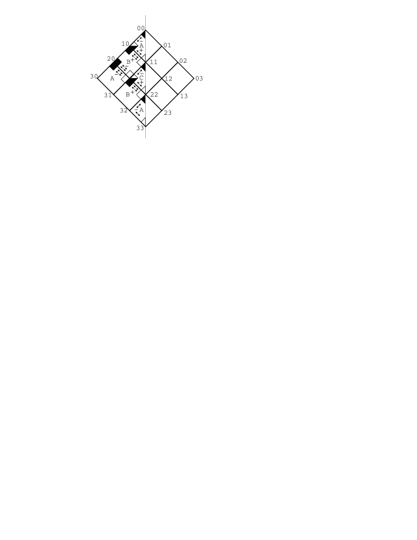
Figure 6: This picture explains the computation of determinants for the term $\int_{X}a\partial\bar{\partial}b_{22}$. The notation is the same as in fig. 5, except that here only $\tilde{a}$ and the $b_{pq}$ are drawn. The picture and the Lagrangian subspace for the antifields $\tilde{b}_{pq}$ and the field $a$ is obtained precisely by 180 degree rotation and flipping black and white colors. The picture encodes the Lagrangian submanifold, and the arrows that represent mappings between various Hilbert spaces of forms. The resulting determinants all cancel except those associated with the three squares on the lower left edge. The result is $A^{-1}BA^{-1}$.

Since the minimal Hitchin model appears to disagree with the $B$-model at one-loop order, we consider now the extended Hitchin functional $H(\phi)$. As we explained in section 2, this functional is defined for a polyform $\phi=\rho_{1}+\rho_{3}+\rho_{3}$. It is constructed by Hitchin [12] in a similar spirit to the minimal Hitchin functional $H(\rho)$ and the action is also given by a square root of a $4^{th}$ order polynomial in $\phi$. The critical points of $H(\phi)$ determine a generalized CY structure[13, 12] on $X$. If $b_{1}(X)$ is trivial, then this generalized CY structure is equivalent to a standard CY structure. The quadratic expansion of the extended Hitchin functional is also given as $\int_{X}\delta\phi\wedge J\delta\phi$, where $J$ is a complex structure on a space of odd polyforms $\phi$ introduced by Hitchin. With respect to the Hodge decomposition of forms, it has $+i$ eigenvalues on the spaces $\Omega^{1,0},\Omega^{3,0},\Omega^{2,1},\Omega^{3,2}$. The quadratic expansion of the extended Hitchin functional near a critical point has the following form

$$S_{cl}=\int_{X}\left(b_{11}\wedge\partial\bar{\partial}b_{11}+b_{00}\wedge\partial\bar{\partial}b_{22}\right).$$ (80)

We need to compute the partition function associated with the second term. It will be helpful to change notation slightly and write $a$ for $b_{00}$, enabling us to reserve the name $b_{00}$ for a ghost field that will arise presently. The classical action is thus

$$S_{cl}=\int a\wedge\partial\bar{\partial}b_{22}.$$ (81)

The gauge invariance is of course $\delta b_{22}=\partial b_{12}+\bar{\partial}b_{21}$. To introduce the BV complex, we begin by introducing the whole collection of ghost fields $b_{pq}$, $p,q\leqslant 2$, with

$$Qb_{22}=\bar{\partial}b_{21}+\partial b_{12}$$ (82)

$$Qb_{21}=\bar{\partial}b_{20}+\partial b_{11},\quad Qb_{12}=\bar{\partial}b_{11}+\partial b_{02}$$

$$Qb_{20}=\partial b_{10},\quad Qb_{11}=\bar{\partial}b_{10}+\partial b_{01},\quad Qb_{02}=\bar{\partial}b_{01}$$

$$Qb_{10}=\partial b_{00},\quad Qb_{01}=\bar{\partial}b_{00}$$

Here $b_{pq}$ has ghost number $4-p-q$ and statistics $(-1)^{p+q}$. Next, we introduce antifields. The antifield for $a$ is a fermionic $(3,3)$-form $\tilde{a}$. The antifields of $b_{pq}$ are fields $\tilde{b}_{3-p,3-q}$, of statistics $(-1)^{p+q+1}$ and ghost number $p+q-5$. The master action is

$$S=S_{cl}+\sum_{p,q}\int\tilde{b}_{3-p,3-q}\wedge Qb_{pq}.$$ (83)

It obeys all the necessary conditions by virtue of the same arguments that we gave in quantizing the original Hitchin Lagrangian. Note that to go from $S_{cl}$ to $S$, we do not add any terms depending on $a$ and $\tilde{a}$, since $a$ is gauge invariant and does not appear on the right hand side of any transformation laws in (82). The transformation laws of antifields under $Q$ can be obtained as $Q\tilde{b}=\{\tilde{b},S\}$, $Q\tilde{a}=\{\tilde{a},S\}$. We will not write them in detail.

The next step is to introduce a Lagrangian submanifold. As in the previous discussion, we do this by projecting each field onto the subspace orthogonal to its variation under a gauge transformation. The evaluation of the path integral is then straightforward, just as we have seen earlier, with each set of fields contributing determinants associated with certain faces of the Hodge diagram. However, the details are lengthy, because there are so many fields. Hence, it is extremely helpful to take a short cut using a figure analogous to fig. 5.

In the fig. 6, we have sketched the various fields and their Hodge decomposition after projection to the Lagrangian submanifold. Each square in the Hodge diamond has an accompanying determinant, which will appear in the partition function with some exponent that we want to compute. The exponent for each square is obtained by counting black regions in that square derived from bosonic or fermionic fields. Many squares do not contribute. For example, the top square in the Hodge diagram has two black triangles, one associated with a bosonic field and one with a fermionic field, so the net exponent is zero. The neighboring square with top corner labeled 10 contains two small black squares, one derived from a bosonic field and one from a fermionic field, so the overall exponent is again zero. The center square has two black triangles, associated with fields of opposite statistics, again giving no net contribution.

Finally, the squares that do contribute are the three squares on the lower left of the Hodge diamond, with left vertex 30, 31, or 32. The square with left vertex 30 contains a small black square derived from a bosonic field, so it contributes a factor $A^{-1}$ to the path integral. The square with left vertex 31 contains a small black square derived from a fermionic field, so it contributes a factor $B$. Finally, the bottom square in the Hodge diagram contains a single black triangle associated with the original bosonic field $b_{22}$. Though a triangle usually gives us an exponent of $\pm 1/2$, in this case $b_{22}$ has a separate conjugate variable, with which it appears in the underlying second order classical action $\int a\partial\bar{\partial}b_{22}$. As there are two fields and a second order action, the factor contributed to the path integral is $A^{-1}$. Putting all this together, the extra factor in the partition function of the extended Hitchin model compared to that of the minimal Hitchin model is $BA^{-2}$.

The result for the partition function of the extended Hitchin model is thus

$$Z_{HE,1-loop}=BA^{-2}Z_{H,1-loop}=A^{-2}B^{2}C^{-1/2},$$ (85)

or equivalently, in terms of torsions,

$$Z_{HE,1-loop}=\frac{I_{1}}{I_{0}^{3}}=\prod_{p=0}^{3}I_{p}^{(-1)^{p}p}.$$ (86)

This agrees with the one-loop partition function of the $B$-model, according to (4).

We summarize the final result in fig. 7.

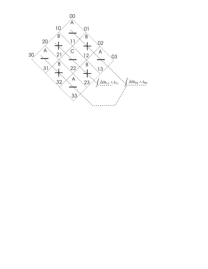
Figure 7: The “chessboard” structure for the powers of “face” determinants is shown for the $Z_{HE,1-loop}=Z_{B,1-loop}$

3 Gravitational Anomaly

Now we want to investigate the dependence of the quantum Hitchin and extended Hitchin models on the background metric that is used for quantization.

This metric is absent in the initial or classical description of the theory, but it has been used to define the Lagrangian submanifold used for quantization and the regularized determinants of Laplace operators. If the resulting partition function depends on the metric, this is an anomaly that seriously affects the physical interpretation of the model.

The dependence of Ray-Singer torsion on the Kahler metric has been determined in [53, 54, 55]. The general formula applies to the torsion of the $\bar{\partial}$ operator with values in any holomorphic vector bundle $V$ on a complex manifold $X$ of complex dimension $n$; for us, the case of interest is $V=\Omega^{p,0}$. The result has been worked out in more detail, for $p=0$, in [56]. In the case of complex dimension one, as was originally elucidated in [57], the dependence of the determinants of Laplacians on the metric reduces to the usual conformal anomaly that appears in Polyakov’s quantization of the bosonic string [58].

We will describe the variation of the torsion with the metric for a general holomorphic vector bundle $V$, and then specialize to the case that $V$ is some $\Omega^{p,0}$. (One reason to begin with the generalization is that it is actually relevant to the $B$-model in the presence of $D$-branes.) We write $g$ for a Kahler metric on $X$ and $h$ for a hermitian metric on $V$. We want to describe the change in the torsion under general deformations $g\to g+t\delta g$, $h\to h+t\delta h$, with $t$ a small parameter and $\delta g$ and $\delta h$ arbitrary small variations (preserving of course the Kahler and hermitian conditions). We write $R$ for the Riemann curvature tensor derived from $g$ and $F$ for the curvature of the connection derived from $h$.

Before trying to present the formula for the variation of the torsion, it helps to develop some notation. As an example, the first Chern class of a holomorphic vector bundle $V$ corresponds to the differential form $c_{1}=\mathop{\rm Tr}(\frac{i}{2\pi}F)$. The curvature $F$ is, of course, a $(1,1)$-form on $X$ with values on $\mathop{\rm End}(V)$. Now we will consider an expression

$$c_{1}(V(t))=\mathop{\rm Tr}\frac{1}{2\pi}\left(iF+th^{-1}\delta h\right).$$ (87)

Here $h^{-1}\delta h$ is a $(0,0)$-form on $X$ with values in endomorphisms of $V$, so after taking the trace we get the sum of a $(1,1)$-form on $X$ and a $(0,0)$-form. We will think of this combination as a first Chern class in an extended sense.

The $t$ derivative of it is

$$\dot{c}_{1}(V(t))=\frac{1}{2\pi}\mathop{\rm Tr}h^{-1}\delta h.$$ (88)

As we see, though the ordinary $c_{1}$ is a $(1,1)$-form, the $t$-derivative of the extended $c_{1}$ is a $(0,0)$-form.

Similarly, for a higher Chern class $c_{k}(V)$, which is defined as a certain homogeneous $k^{th}$ order function of $\frac{i}{2\pi}F$, we define an extended, $t$-dependent version $c_{k}(V(t))$ by replacing $iF$ with $iF+th^{-1}\delta h$. Then $\dot{c}_{k}(V(0))$ is a $(k-1,k-1)$-form, though the ordinary $c_{k}(t)$ is of course a $(k,k)$-form.

For a general characteristic class like the Todd class $\mathop{\rm Td}(TX)$ or the Chern character $\mathop{\rm Ch}(V)$, we write $\mathop{\rm Td}(TX)_{k}$ or $\mathop{\rm Ch}(V)_{k}$ for the components of degree $(k,k)$. These functions are expressed as homogeneous polynomials of degree $k$ in the curvatures $\frac{i}{2\pi}R$ and $\frac{i}{2\pi}F$, so we can define $t$-dependent generalizations by replacing $iR$ by $iR+tg^{-1}\delta g$ and $iF$ by $iF+th^{-1}\delta h$. Clearly, then, $\left.\frac{\partial}{\partial t}\mathop{\rm Td}(TX)_{k}\right|_{t=0}$ is of degree $(k-1,k-1)$, and likewise if we replace $\mathop{\rm Td}(X)$ by $\mathop{\rm Ch}(V)$ or a product of similar expressions. For a general holomorphic vector bundle $V$, one defines

$$c(V)\equiv c\left(\frac{i}{2\pi}F\right)=\mathop{\rm det}\nolimits\left(1+\frac{i}{2\pi}F\right)=\prod_{i=1}^{r}(1+x_{i})=\sum_{k=0}^{r}c_{k}(V),$$ (89)

where $x_{i}$ are the formal eigenvalues of $\frac{i}{2\pi}F$ and $r=\mathop{\rm rank}\nolimits(V)$. So

$$c_{k}(V)=\sum_{i_{1}<i_{2}<\dots i_{k}}x_{i_{1}}x_{i_{2}}.\dots x_{i_{k}}$$ (90)

Then

$$\mathop{\rm Td}(V)=\prod_{i=1}^{r}\frac{x_{i}}{1-e^{-x_{i}}},\quad\mathop{\rm Ch}(V)=\sum_{i=1}^{r}e^{x_{i}}$$ (91)

According to Theorem 1.22 in [55], the variation of the torsion under a change in Kahler metric is given by

$$\frac{1}{2\pi}\left.\frac{\partial}{\partial t}\right|_{t=0}\log I(X,V,g,h)=\frac{1}{2}\int_{X}\frac{\partial}{\partial t}\left[\mathop{\rm Td}\frac{1}{2\pi}(iR+tg^{-1}\delta g)\mathop{\rm Ch}\frac{1}{2\pi}(iF+th^{-1}\delta h)\right]_{n+1}.$$ (92)

For the closed string $B$-model, we specialize to the case that $V$ is a sum of bundles $\Omega^{p,0}$, $F$ coincides with $R$ (written of course in the appropriate representation $\Omega^{p,0}=\mathop{\bigwedge}\nolimits^{p}{T^{*}X})$ and $h$ is determined by $g$.

For the $B$-model or equivalently the extended Hitchin model at one-loop, one has

$$F_{1}^{B}=-\sum_{p=0}^{n}(-1)^{p}p\,\log I(X,\Omega^{p,0}),$$ (93)

where we do not indicate the dependence on the metric explicitly. The anomaly of the ordinary Hitchin model can of course be studied in a similar way, but apparently does not lead to such simple formulas. We will omit this case.

To compute the variation of $F_{1}^{B}$ using  (92), it is first convenient to algebraically simplify the characteristic class entering into the variation of $F_{1}$. This class is

$$P=\sum_{p=0,\dots,n}p(-1)^{p}\mathop{\rm Td}(TX)\mathop{\rm Ch}(\wedge^{p}T^{*}X),$$ (94)

where $TX$ is the holomorphic tangent bundle of $X$, and $T^{*}X$ is its dual. A simple expression for $P$ was obtained in [8], where it arose for reasons closely related to our present discussion.

Let $x_{i}$ be the Chern roots of $TX$ (the formal eigenvalues of $\frac{i}{2\pi}R$, where $R$ is the curvature of $TX$). The Chern roots of $\wedge^{p}T^{*}X$ are $-x_{i_{1}}-x_{i_{2}}-\dots-x_{i_{p}}$, $i_{1}<i_{2}<\dots<i_{p}$. So the Chern character of $\wedge^{p}T^{*}X$ is $\sum_{i_{1}<\cdots<i_{p}}e^{-x_{i_{1}}-x_{i_{2}}-\dots-x_{i_{p}}}$.

We have then

$$\sum_{p=0}^{n}(-1)^{p}p\mathop{\rm Ch}(\wedge^{p}T^{*}X) =\sum_{p=0,\dots,n}p(-1)^{p}\sum_{i_{1}<\cdots<i_{p}}e^{-x_{i_{1}}-x_{i_{2}}-\dots-x_{i_{p}}}$$ (95)

$$=\partial_{z}\prod_{i=1}^{n}(1-ze^{-x_{i}})|_{z=1}=-\sum_{j=1,\dots,n}e^{-x_{j}}\prod_{\begin{subarray}{c}i=1,\dots,n\\ i\neq j\end{subarray}}(1-e^{-x_{i}}).$$

Hence, after multiplying by the Todd class to get $P$, we have

$$P =-\prod_{i=1}^{n}x_{i}\sum_{j=1}^{n}\frac{e^{-x_{j}}}{1-e^{-x_{j}}}=\sum_{j=1}^{n}\frac{x_{j}}{1-e^{x_{j}}}\prod_{\begin{subarray}{c}i=1,\dots,n\\ i\neq j\end{subarray}}x_{i}=-\sum_{j=1}^{n}\left(1-\frac{x_{j}}{2}+\frac{x_{j}^{2}}{12}+\dots\right)\prod_{\begin{subarray}{c}i=1,\dots,n\\ i\neq j\end{subarray}}x_{i}$$ (96)

$$=-\left(c_{n-1}-\tfrac{n}{2}c_{n}+\tfrac{1}{12}c_{n}c_{1}+\dots\right)$$

The component of degree $n+1$ is equal simply to $-\tfrac{1}{12}c_{n}c_{1}$.

Plugging this into the variational formula (92), one has

$$\frac{1}{2\pi}\frac{\partial}{\partial t}F_{1}(g+t\delta g)=-\frac{1}{24}\int_{X}\partial_{t}(c_{n}c_{1}).$$ (97)

As we have already discussed, the $t$ derivative of $c_{1}(TX(t))$ is given by

$$\dot{c}_{1}=\frac{1}{2\pi}\mathop{\rm Tr}g^{-1}\delta g$$ (98)

The derivative $c_{n}$ can be similarly expressed in terms of $\mathop{\rm Tr}R^{k}g^{-1}\delta g$, but one does not need the explicit expressions to see that generally, for an arbitrary metric $g$ and an arbitrary variation $\delta g$, the total variation $\int_{X}\partial_{t}(c_{n}c_{1})$ is nonzero and more seriously, is not a function only of the Kahler class.

Consider a general variation of the metric that does not change the Kahler class. Thus, $\delta g=\partial\bar{\partial}u$, for some function $u$, and $\mathop{\rm Tr}g^{-1}\delta g=\Delta u$, $\Delta$ being the Laplacian. If the complex dimension of $X$ is $n=1$, the variation of $F_{1}$ involves

$$\int_{X}\partial_{t}(c_{1}^{2})=2\frac{1}{2\pi}\int_{X}c_{1}\Delta u.$$ (99)

In general $c_{1}$ is a completely arbitrary $(1,1)$ curvature form whose integral is zero, and $u$ is an arbitrary function; this expression certainly does not vanish in general. Similarly, for complex dimension three, the anomaly does not vanish in general. For example, if one takes $X$ to be the product of a K3 surface and an elliptic curve $E$, with a fixed Ricci-flat metric on K3 and a varying Kahler metric on $E$, then the anomaly computation reduces to what we have just described. So the $B$-model or extended Hitchin model is anomalous at one-loop order.

We really do not know how to interpret this result in general. However, we can make one mildly comforting remark: the variation of the one-loop $B$-model partition function with respect to the metric is a function only of the Kahler class if evaluated for a Ricci-flat Kahler metric $g$ and a deformation $\delta g$ that preserves the Ricci-flatness. To show this, first note that the Ricci-flat condition means that the $(1,1)$-form representing $c_{1}$ is zero pointwise on $X$. So if we compute at a Ricci-flat Kahler metric, the variation of $\frac{1}{2\pi}F_{1}^{B}$ is

$$\frac{1}{2\pi}\frac{\partial}{\partial t}F_{1}(g+t\delta g)=-\frac{1}{24}\int_{X}c_{n}\dot{c}_{1},$$ (100)

so

$$\delta F^{B}_{1}=-\frac{1}{24}\int_{X}c_{n}\mathop{\rm Tr}g^{-1}\delta g$$ (101)

But as we will now show, if we vary the metric in a way that preserves the Ricci-flat condition, then $\dot{c}_{1}$ is also simple, and the derivative of $F_{1}^{B}$ with respect to the Kahler moduli is only a function of the Kahler moduli, not the complex structure moduli. Moreover, the Kahler moduli enter only via the volume of $X$. This means that as long as we compute only for Ricci-flat metrics, we can remove the anomaly, somewhat artificially, by multiplying the one-loop partition function by a factor that only depends on Kahler moduli, in fact, only on the volume of $X$.

So consider a variation $\delta g$ of the Kahler metric, which preserves the Ricci-flat condition while (inevitably) changing the Kahler class. Since the variation of the Ricci tensor

$$R_{i\bar{j}}=-\partial_{i}\partial_{\bar{j}}\log\mathop{\rm det}\nolimits g$$ (102)

must vanish, one has the condition on variation $\delta g$:

$$\partial_{i}\partial_{\bar{j}}\mathop{\rm Tr}g^{-1}\delta g=0.$$ (103)

Hence if $X$ is compact or suitable boundary conditions are placed at infinity, then $\mathop{\rm Tr}g^{-1}\delta g$ is constant on $X$, and hence can be identified with the change in the volume:

$$\mathop{\rm Tr}g^{-1}\delta g=2\delta\log{\rm Vol(X)}.$$ (104)

So the formula for variation of $F_{1}$ simplifies to

$$\delta F_{1}=-\frac{1}{24}\mathop{\rm Tr}(g^{-1}\delta g)\int_{X}c_{n}=-\frac{1}{12}\delta\log{\rm Vol}(X)\chi(X)$$ (105)

Hence for $Ricci$ flat metric preserving variations

$$Z_{B,1-loop}{\rm Vol}(X)^{-\chi/12}.$$ (106)

is independent of the Kahler moduli of $X$. We should note, however, that in this paper we have not very well understood the physical meaning of the zero modes that appear in quantizing the various actions that we have considered – especially the zero modes for ghosts and antifields. Since the volume of $X$ is a function of the zero modes (of the physical fields), it may be that the physical meaning of the volume factor in (106) really needs to be considered along with the physics of the zero modes. At any rate, we recall that mathematically, when zero modes are present, the torsion, and hence $Z_{B,1-loop}$, is not a number but a measure on the space of zero modes.

One additional simple remark is that the anomaly suggests that one should embed the $B$-model and the extended Hitchin model in a target space theory which involves the Kahler metric and produces a Ricci-flat metric in its critical points. An obvious candidate is the Hitchin functional in seven dimensions that leads at its critical points to metrics of $G_{2}$ holonomy, specialized to seven-manifolds of the form $X\times S^{1}$. This idea is in accord with the philosophy proposed in [1, 2, 3, 4, 12].

4 Conclusion

The Hitchin functionals are closely related to topological strings in target space as has been demonstrated at tree level  [1, 2, 3].

The first quantum effects appear in one-loop order. The quadratic computation has been made in the present work using the Batalin-Vilkovisky formalism, for which it is well adapted because of the presence of redundant or reducible gauge transformations. The result shows that the minimal Hitchin model does not agree at one-loop order with the conjecture of [1], but the extended Hitchin model does.

A puzzle remains. The one-loop $B$-model or extended Hitchin model appears to possess an anomaly with respect to changes in the Kahler metric.

- [1] R. Dijkgraaf, S. Gukov, A. Neitzke, and C. Vafa, Topological -Theory as Unification of Form Theories of Gravity, hep-th/0411073.
- [2] A. A. Gerasimov and S. L. Shatashvili, Towards Integrability of Topological Strings. i: Three-Forms on Calabi-Yau Manifolds, JHEP 11 (2004) 074, [hep-th/0409238].
- [3] N. Nekrasov, A la Recherche de la M-Theorie Perdue. Z Theory: Casing Theory, hep-th/0412021.
- [4] N. Hitchin, The Geometry of Three-Forms in Six Dimensions, J. Differential Geom. 55 (2000), no. 3 547–576.
- [5] E. Witten, Mirror Manifolds and Topological Field Theory, hep-th/9112056.
- [6] E. Witten, Topological Sigma Models, Commun. Math. Phys. 118 (1988) 411.
- [7] E. Witten, Topological Quantum Field Theory, Commun. Math. Phys. 117 (1988) 353.
- [8] M. Bershadsky, S. Cecotti, H. Ooguri, and C. Vafa, Kodaira-Spencer Theory of Gravity and Exact Results for Quantum String Amplitudes, Commun. Math. Phys. 165 (1994) 311–428, [hep-th/9309140].
- [9] H. Ooguri, A. Strominger, and C. Vafa, Black Hole Attractors and the Topological String, Phys. Rev. D70 (2004) 106007, [hep-th/0405146].
- [10] C. Vafa, Two Dimensional Yang-Mills, Black Holes and Topological Strings, hep-th/0406058.
- [11] M. Aganagic, H. Ooguri, N. Saulina, and C. Vafa, Black Holes, -Deformed 2d Yang-Mills, and Non-Perturbative Topological Strings, hep-th/0411280.
- [12] N. Hitchin, Generalized Calabi-Yau manifolds, Q. J. Math. 54 (2003), no. 3 281–308.
- [13] M. Gualtieri, Generalized Complex Geometry, Oxford University DPhil thesis (2004) [math.DG/0401221].
- [14] M. Grana, R. Minasian, M. Petrini, and A. Tomasiello, Supersymmetric Backgrounds From Generalized Calabi-Yau Manifolds, JHEP 08 (2004) 046, [hep-th/0406137].
- [15] U. Lindstrom, R. Minasian, A. Tomasiello, and M. Zabzine, Generalized Complex Manifolds and Supersymmetry, hep-th/0405085.
- [16] S. Gurrieri, J. Louis, A. Micu, and D. Waldram, Mirror Symmetry in Generalized Calabi-Yau Compactifications, Nucl. Phys. B654 (2003) 61–113, [hep-th/0211102].
- [17] S. Fidanza, R. Minasian, and A. Tomasiello, Mirror Symmetric -Structure Manifolds with NS Fluxes, Commun. Math. Phys. 254 (2005) 401–423, [hep-th/0311122].
- [18] A. Kapustin, Topological Strings on Noncommutative Manifolds, Int. J. Geom. Meth. Mod. Phys. 1 (2004) 49–81, [hep-th/0310057].
- [19] A. Kapustin and Y. Li, Topological Sigma-Models with -Flux and Twisted Generalized Complex Manifolds, hep-th/0407249.
- [20] A. Kapustin and Y. Li, Open String BRST Cohomology for Generalized Complex Branes, hep-th/0501071.
- [21] M. Zabzine, Geometry of -Branes for General Sigma Models, hep-th/0405240.
- [22] M. Zabzine, Hamiltonian Perspective on Generalized Complex Structure, hep-th/0502137.
- [23] R. Zucchini, Generalized Complex Geometry, Generalized Branes and the Hitchin Sigma Model, hep-th/0501062.
- [24] C. Jeschek and F. Witt, Generalised -Structures and Type IIB Superstrings, hep-th/0412280.
- [25] S. Chiantese, Isotropic -Branes and the Stability Condition, JHEP 02 (2005) 003, [hep-th/0412181].
- [26] S. Chiantese, F. Gmeiner, and C. Jeschek, Mirror Symmetry for Topological Sigma Models with Generalized Kaehler Geometry, hep-th/0408169.
- [27] N. Ikeda, Three Dimensional Topological Field Theory Induced From Generalized Complex Structure, hep-th/0412140.
- [28] C. Jeschek, Generalized Calabi-Yau Structures and Mirror Symmetry, hep-th/0406046.
- [29] C. C. Chevalley, The Algebraic Theory of Spinors. Columbia University Press, New York, 1954.
- [30] N. Berkovits and D. Z. Marchioro, Relating the Green-Schwarz and Pure Spinor Formalisms for the Superstring, JHEP 01 (2005) 018, [hep-th/0412198].
- [31] P. Grange and R. Minasian, Modified Pure Spinors and Mirror Symmetry, hep-th/0412086.
- [32] A. S. Schwarz, The Partition Function of a Degenerate Functional, Comm. Math. Phys. 67 (1979), no. 1 1–16.
- [33] A. S. Schwarz, The Partition Function of Degenerate Quadratic Functional and Ray-Singer Invariants, Lett. Math. Phys. 2 (1977/78), no. 3 247–252.
- [34] D. B. Ray and I. M. Singer, -Torsion and the Laplacian on Riemannian Manifolds, Advances in Math. 7 (1971) 145–210.
- [35] D. B. Ray and I. M. Singer, Analytic Torsion, in Partial Differential Equations (Proc. Sympos. Pure Math., Vol. XXIII, Univ. California, Berkeley, Calif., 1971), pp. 167–181. Amer. Math. Soc., Providence, R.I., 1973.
- [36] D. B. Ray and I. M. Singer, Analytic Torsion for Complex Manifolds, Ann. of Math. (2) 98 (1973) 154–177.
- [37] E. Witten, Chern-Simons Gauge Theory as a String Theory, Prog. Math. 133 (1995) 637–678, [hep-th/9207094].
- [38] E. Witten, Quantization of Chern-Simons Gauge Theory with Complex Gauge Group, Commun. Math. Phys. 137 (1991) 29–66.
- [39] S. Axelrod, S. Della Pietra, and E. Witten, Geometric Quantization of Chern-Simons Gauge Theory, J. Diff. Geom. 33 (1991) 787–902.
- [40] S. Axelrod and I. M. Singer, Chern-simons Perturbation Theory, hep-th/9110056.
- [41] S. Axelrod and I. M. Singer, Chern-Simons Perturbation Theory. 2, J. Diff. Geom. 39 (1994) 173–213, [hep-th/9304087].
- [42] A. S. Cattaneo, Abelian Theories and Knot Invariants, Comm. Math. Phys. 189 (1997), no. 3 795–828.
- [43] A. S. Cattaneo and C. A. Rossi, Higher-Dimensional Theories in the Batalin-Vilkovisky Formalism: the BV Action and Generalized Wilson Loops, Comm. Math. Phys. 221 (2001), no. 3 591–657.
- [44] A. Schwarz, Topological Quantum Field Theories, hep-th/0011260.
- [45] A. Schwarz, Geometry of Batalin-Vilkovisky Quantization, Commun. Math. Phys. 155 (1993) 249–260, [hep-th/9205088].
- [46] E. Witten, Quantum Field Theory and the Jones Polynomial, Commun. Math. Phys. 121 (1989) 351.
- [47] I. A. Batalin and G. A. Vilkovisky, Gauge Algebra and Quantization, Phys. Lett. B102 (1981) 27–31.
- [48] I. A. Batalin and G. A. Vilkovisky, Quantization of Gauge Theories with Linearly Dependent Generators, Phys. Rev. D28 (1983) 2567–2582.
- [49] M. Henneaux, Lectures on the Antifield-BRST Formalism for Gauge Theories, Nucl. Phys. Proc. Suppl. 18A (1990) 47–106.
- [50] E. Witten, A Note on the Antibracket Formalism, Mod. Phys. Lett. A5 (1990) 487.
- [51] M. Bochicchio, Gauge Fixing for the Field Theory of the Bosonic String, Phys. Lett. B193 (1987) 31.
- [52] P. Griffiths and J. Harris, Principles of Algebraic Geometry. Wiley-Interscience [John Wiley & Sons], New York, 1978. Pure and Applied Mathematics.
- [53] J.-M. Bismut, H. Gillet, and C. Soulé, Analytic Torsion and Holomorphic Determinant Bundles. I. Bott-Chern forms and analytic torsion, Comm. Math. Phys. 115 (1988), no. 1 49–78.
- [54] J.-M. Bismut, H. Gillet, and C. Soulé, Analytic Torsion and Holomorphic Determinant Bundles. II. Direct Images and Bott-Chern forms, Comm. Math. Phys. 115 (1988), no. 1 79–126.
- [55] J.-M. Bismut, H. Gillet, and C. Soulé, Analytic Torsion and Holomorphic Determinant Bundles. III. Quillen Metrics on Holomorphic Determinants, Comm. Math. Phys. 115 (1988), no. 2 301–351.
- [56] W. Müller and K. Wendland, Extremal Kähler Metrics and Ray-Singer Analytic Torsion, in Geometric aspects of partial differential equations (Roskilde, 1998), vol. 242 of Contemp. Math., pp. 135–160. Amer. Math. Soc., Providence, RI, 1999.
- [57] A. A. Belavin and V. G. Knizhnik, Algebraic Geometry and the Geometry of Quantum Strings, Phys. Lett. B168 (1986) 201–206.
- [58] A. M. Polyakov, Quantum Geometry of Bosonic Strings, Phys. Lett. B103 (1981) 207–210.